a framework to assess the risks to human health and the
TRANSCRIPT
A Framework to Assess the Risksto Human Health and theEnvironmentfrom Landfill Gas
WS Atkins Environment
R&D Technical Report P271
A Framework to Assess the Risksto Human Health and the Environmentfrom Landfill Gas
R G Gregory, A J Revans, M D Hill,M P Meadows, L Paul and C C Ferguson
Research contractor:WS Atkins Environment
Environment AgencyRio HouseWaterside DriveAztec WestAlmondsburyBristol BS32 4UD
Commissioning OrganisationEnvironment AgencyRio HouseWaterside DriveAztec WestAlmondsburyBristol BS32 4UD
Tel: 01454 624400 Fax: 01454 624409
Environment Agency CWM 168/98 ISBN 1 85705 254 4
All rights reserved. No part of this document may be produced, stored in a retrieval system, ortransmitted, in any form or by any means, electronic, mechanical, photocopying, recording, orotherwise without the prior permission of the Environment Agency.
The views expressed in this document are not necessarily those of the Environment Agency. Itsofficers, servants or agents accept no liability whatsoever for any loss or damage arising from theinterpretation or use of the information, or reliance upon views contained herein.
Dissemination statusInternal: Released to RegionsExternal: Public Domain
Statement of useThis R&D technical report documents the development of a framework for a landfill gas riskassessment tool to help the Environment Agency and others assess the human health andenvironmental risks of landfill gas emissions from landfill sites. The HELGA model is currentlybased in Microsoft Excel 97TM and requires further development before being released internallyand externally complete with User Manual. R&D Technical Summary PS257 is also availableand is related to this report.
Research contractorThis document was produced under R&D Project P1-283 (contract HOCO_225) by:
WS Atkins EnvironmentWoodcote GroveAshley RoadEpsom KT18 5BW Tel: 01372 726140 Fax: 01372 740055
The sub-contractor was:
CRBEThe Nottingham Trent UniversityBurton StreetNottingham NG1 4BU
Environment Agency’s Project ManagerThe Environment Agency’s Project Manager for R&D Project P1-283 was:Louise McGoochan - Southern Region

A Framework to Assess the Risks to Human Health and the Environment from Landfill Gas
R&D Technical Report P271 i
SUMMARY
This is the final report for R&D Project P1-283; A Framework to Assess the Risks to HumanHealth and the Environment from Landfill Gas. The project has delivered a model frameworkentitled HELGA (Health and Environmental risks form Landfill GAs), to help the EnvironmentAgency assess the risks to human health and the environment from landfill gas (LFG).HELGA is a demonstration framework to test the feasibility of a fully developed model. Whendeveloped to commercial standards, the code is expected to be complementary to LANDSIM,the Environment Agency’s risk assessment model for leachate migration into groundwater.
The HELGA model contain ten related modules:
1. Source term gas generation;2. Emissions;3. Atmospheric dispersion;4. Lateral migration;5. Migration into houses;6. Human exposure;7. Odour;8. Vegetation stress;9. Global atmospheric risk; and10. a summary Output module.
The foundation of the model is a source term module, which is a flexible landfill gas (LFG)generation model that the user can tailor to an individual landfill site. The user can define thewaste composition in terms of various waste streams, including inter alia, municipal,commercial, industrial and inert waste types, the era in which the waste was emplaced (toreflect compositional changes in different decades) and the moisture content of the waste.
These waste characteristics then feed into a first-order decay model that estimates LFGgeneration for up to 150 years. Programming limitations exist when combining the MicrosoftExcel™ spreadsheet and Crystal Ball™ probabilistic risk assessment software, which limits themodel working in a fully probabilistic mode. Therefore the source term module has beendesigned to be pseudo probabilistic. This means that ranges for gas generation forecasts,perhaps the most uncertain data to be generated by the model, have been sampled using theCrystal Ball™ Monte-Carlo sampling package, and the 95th, 50th and 5th percentile results forgas generation per tonne of waste have been set as constants in a look-up table. The user canchoose which set of forecasts (95th, 50th or 5th percentiles) to use with the other user definedparameters, to give a maximum, average or minimum result for the outputs from the model.
The Emissions module takes the output (for 95th, 50th or 5th percentiles) of the source-termmodule for a specified year and uses it to calculate LFG flux to the environment after allowingfor gas collection, flaring, energy recovery and biological methane oxidation. This moduleuses information on the site gas collection system, flare and engine, cap and liner (if any) tocalculate for a given year what proportion of the gas generated is emitted via each route. LFGgenerated and not collected is assumed to be in equilibrium with that emitted from the landfillcap or liner at a steady state.

A Framework to Assess the Risks to Human Health and the Environment from Landfill Gas
R&D Technical Report P271 ii
The Atmospheric Dispersion module is in two parts:
• Atmospheric dispersion off site; and• Atmospheric dispersion on site (only for worker exposure).
The off site dispersion module uses a Gaussian plume model that has some probabilisticaspects incorporated, and includes; chemical deposition, wind direction, flare plume buoyancyand atmospheric layer stability. On-site dispersion is calculated using a simple box model, andthis gives a good approximation of exposure on site.
The lateral migration module comprises a diffusion model that uses a concentration gradient todrive LFG migration. The model accounts for the physical characteristics of the soil and gasesor VOCs, and distance to the receptor. The model does not account for advective flow ormethane oxidation in the ground due to a dearth of available information. The risk from amigration event is accounted for by examining the occurrence of various scenarios that maylead to advective flow through fractures in permeable ground.
Migration into houses is simulated to allow for gas entry via the ground and the atmosphere.There are two different types of building considered; those with suspended floors or cellars,and those with a slab floor design.
The exposure assessment module focuses on calculating intakes of pollutants by members ofthe public through three main routes; ingestion, inhalation, and dermal exposure. The dataused for these modules comes mainly from work carried out by NRPB, with some informationfrom other US or EU sources.
The odour module compares the chemical odour threshold with the concentration in air at thereceptor. Similarly, the vegetation stress module compares the concentration of methane andcarbon dioxide in the ground at the receptor with the concentration where vegetation stress isfirst observed.
The global atmospheric risk module uses the total emissions (including VOCs) from the site ina specified year to calculate the corresponding ozone depletion potential (ODP) and globalwarming potential (GWP). These figures can be compared with other model runs on the samesite with different cap designs and gas management options to evaluate the best combination ofgas management options for the environment.
The Output Module collates the results from the various modules in the spreadsheetworkbook, and presents them in an easy to understand tabular form.
Validation of the model has been carried out on five landfills, to evaluate key outputs in themodel. In all cases, the forecasts are in good agreement with observed measurements. FourScenarios have also been developed to demonstrate how decisions on landfill gas cap design,flaring and gas utilisation can be made to optimise LFG emissions to the benefit of the localand global environment and human health. These scenarios demonstrate that good cap designtogether with gas collection and flaring and/or gas utilisation reduce global environmentalrisks, and generally reduce local human health risks. The only emissions to increase as a resultof gas utilisation are the engine emission products, and these are not forecast to be generatedin sufficient quantity to appear to be a health risk.

A Framework to Assess the Risks to Human Health and the Environment from Landfill Gas
R&D Technical Report P271 iii
CONTENTS
1. INTRODUCTION ............................................................................................................1
1.1 Purpose of this report .....................................................................................................11.2 Background to project....................................................................................................11.3 Aim of project .................................................................................................................21.4 Summary of project tasks...............................................................................................2
2. CONCEPTUAL MODEL ................................................................................................3
2.1 Intended use and limitations of the model.....................................................................32.2 Wastes considered in the model .....................................................................................52.3 Source term modelling....................................................................................................72.4 Selection of pollutants to be modelled............................................................................8
2.4.1 Bulk gases.................................................................................................................82.4.2 Trace gases and VOCs.............................................................................................92.4.3 Surface emissions .....................................................................................................92.4.4 Lateral emissions......................................................................................................92.4.5 Flare emissions ....................................................................................................... 102.4.6 Utilisation plant emissions..................................................................................... 102.4.7 Odour ..................................................................................................................... 10
2.5 Pathways and targets.................................................................................................... 102.6 Probabilistic aspects ..................................................................................................... 11
3. SOURCE TERM ............................................................................................................ 14
3.1 Landfill gas generation................................................................................................. 143.1.1 Module description ................................................................................................ 15
3.2 Using the source term module...................................................................................... 193.2.1 QA sheet ................................................................................................................. 213.2.2 Input sheet ............................................................................................................. 213.2.3 Wastes 1 - 4 ............................................................................................................ 233.2.4 Waste water content .............................................................................................. 233.2.5 Defaults and data................................................................................................... 233.2.6 Data manipulation ................................................................................................. 243.2.7 LFG production ..................................................................................................... 26
3.3 Landfill gas emissions................................................................................................... 273.3.1 Landfill gas data .................................................................................................... 273.3.2 Flare Input ............................................................................................................. 303.3.3 Utilisation............................................................................................................... 333.3.4 Water content of the waste.................................................................................... 343.3.5 Emission route ....................................................................................................... 343.3.6 Model output.......................................................................................................... 34
4. ENVIRONMENTAL TRANSPORT ............................................................................. 36
4.1 Atmospheric dispersion off-site.................................................................................... 364.1.1 Types of models and sources ................................................................................. 364.1.2 User input............................................................................................................... 364.1.3 Equations and parameter values........................................................................... 374.1.4 Output .................................................................................................................... 43
A Framework to Assess the Risks to Human Health and the Environment from Landfill Gas
R&D Technical Report P271 iv
4.2 Atmospheric dispersion on-site .................................................................................... 434.3 Lateral migration under steady state conditions......................................................... 444.4 Lateral migration in unusual conditions ..................................................................... 45
5. EXPOSURE ASSESSMENT ......................................................................................... 46
5.1 Intakes of pollutants by members of the public and site workers............................... 465.1.1 Inhalation exposure model .................................................................................... 475.1.2 Ingestion exposure model ...................................................................................... 505.1.3 Dermal exposure model ......................................................................................... 55
5.2 Calculation of pollutant concentrations in indoor air ................................................. 55
6. VALIDATION TESTS FOR THE HELGA MODULES ............................................. 60
6.1 Introduction.................................................................................................................. 606.2 Validation of the gas generation module ..................................................................... 61
6.2.1 Assumptions........................................................................................................... 616.2.2 Validation Results.................................................................................................. 62
6.3 Validation of gas generation module and surface emission of methane ..................... 656.3.1 Assumptions........................................................................................................... 656.3.2 Validation results ................................................................................................... 65
6.4 Validation of surface emissions module for VOCs ...................................................... 686.4.1 Assumptions........................................................................................................... 686.4.2 Validation results ................................................................................................... 68
6.5 Validation of atmospheric dispersion module ............................................................. 716.5.1 Assumptions........................................................................................................... 716.5.2 Validation results ................................................................................................... 71
6.6 Validation of Lateral Migration................................................................................... 736.6.1 Assumptions........................................................................................................... 736.6.2 Model outputs ........................................................................................................ 73
6.7 Conclusions from validation tests ................................................................................ 756.7.1 Comparison with observations.............................................................................. 756.7.2 Uncertainties and deficiencies in the model.......................................................... 75
7. LFG EMISSIONS MANAGEMENT OPTIONS .......................................................... 76
7.1 Introduction.................................................................................................................. 767.2 Results of gas generation simulations .......................................................................... 79
7.2.1 Gas generation ....................................................................................................... 797.2.2 Potential for gas migration through cap and liner ............................................... 797.2.3 Methane oxidation in the cap................................................................................ 82
7.3 Global environmental burdens..................................................................................... 827.4 VOC emissions.............................................................................................................. 837.5 Results of site worker exposure simulations ................................................................ 857.6 Results of offsite inhalation exposure simulations....................................................... 877.7 Conclusions ................................................................................................................... 88
8. REFERENCES............................................................................................................... 90

A Framework to Assess the Risks to Human Health and the Environment from Landfill Gas
R&D Technical Report P271 1
1. INTRODUCTION
1.1 Purpose of this report
This is the technical report for Environment Agency R&D Project P1-283:
A Framework to Assess the Risks to Human Health and the Environment from Landfill Gas.
This report describes the methodology used in the development of a framework for riskassessment, and the implementation of this framework as a spreadsheet model, HELGA(Health and Environmental Risks from Landfill GAs). The model allows both landfill siteoperators and regulators to review and plan landfill gas management techniques to benefithuman health and the environment. This final report is designed for widespread disseminationamongst the waste management community. The project commenced in August 1997 and thetechnical work was completed in August 1998. Since that period, the model has been trialledamongst the project steering group members.
1.2 Background to project
The Waste Management and Regulation Policy Group (WMRPG) of the Environment Agencyfor England and Wales (the Agency) recruited this project on behalf of the Agency’s NationalWaste Group. The project was designed to assist waste regulators, local authority plannersand landfill site operators, amongst others, to assess the risks to human health and theenvironment associated with landfill gas (LFG) emissions. In addition, the project wasintended to help the Agency and other relevant organisations compare the relative risksassociated with different waste management options, and provide a framework that willcontribute to the assessment and valuation of the inventory of burdens associated withlandfilling of wastes.
The work has been undertaken under the guidance of the Landfill Gas Task and FinishWorking Group, set up under the National Waste Group of the Agency to review currentguidance on LFG and to develop new guidance as required. Members of the working groupformed a steering group for the project. The Landfill Gas Group is responsible for reviewinginternal guidance and, for example, to consider appropriate revisions to Waste ManagementPaper 27 (DoE, 1991). This group is therefore the expert centre on LFG issues.
Members of the Landfill Gas Task and Finish Working Group are:
John Keenlyside Anglian RegionJan Gronow Head OfficeRichard Smith Head OfficeTrevor Howard Midlands RegionIan Cowie North East Region (Chair)Dave Walmsley North West RegionLouise McGoochan Southern Region

A Framework to Assess the Risks to Human Health and the Environment from Landfill Gas
R&D Technical Report P271 2
Catriona Bogan South West RegionAlan Rosevear Thames RegionPete Stanley Environment Agency, WalesRowland Douglas Scottish Environment Protection Agency (SEPA)
This project focused on:
• the risks associated with LFG from waste disposal by landfill;• explosion and fire hazards from accumulation of landfill methane in buildings or
other enclosed spaces;• harm to both the local and global environment.
The project complements the following Environment Agency R&D Projects:
• an assessment of the risks to human health from landfilling of household wastesR&D Project P1-236;
• a risk assessment methodology for landfills (LANDSIM) R&D Project P1-294.
1.3 Aim of project
The overall aim of this project was to develop a useable framework model to help Agency staffassess the risks to human health and the environment from landfill gas. The framework thatwas developed consists of spreadsheet modules integrated to provide a working model, whichmay eventually be developed into a package comparable in style and approach to the Agency’sLANDSIM risk assessment methodology for landfills and groundwater protection.
1.4 Summary of project tasks
The project comprised a number of specific tasks, designed to address the objectives of theproject brief.
• Task 1, Development of the conceptual model. This is described in Chapter 2.
• Task 2, Development of the source term model. This is described in Chapter 3.
• Task 3, Environmental transport models. These are described in Chapter 4.
• Task 4, Exposure assessment. This is described in Chapter 5.
• Task 5, Impact assessment. This is described in Chapter 6.
• Task 6, Validation, simulation and option evaluation. Validation of the model frameworkis described in Chapter 7. Simulation and options evaluation is carried out in Chapter 8.

A Framework to Assess the Risks to Human Health and the Environment from Landfill Gas
R&D Technical Report P271 3
• Task 7, A user manual for the spreadsheet. This task has been reported separately fromthis report, in the form of a user manual and training day programme for Agency staff onthe Task and Finish Group.
These tasks 1-6 are described in the subsequent Chapters of this report.

A Framework to Assess the Risks to Human Health and the Environment from Landfill Gas
R&D Technical Report P271 3
2. CONCEPTUAL MODEL
This Chapter describes the broad approach adopted for the simulation of LFG emissions.More detailed descriptions of the approach to each module within the model itself are given insubsequent sections of this report. This section covers:
• intended use and limitations of the model;• choice of wastes to be considered;• the generation and emission of gases and trace components (the source term);• choice of pollutants to be considered;• pathways and targets; and• probabilistic aspects of the model.
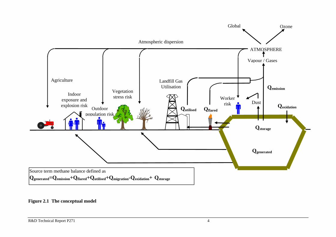
Figure 2.1 shows the sources, pathways, and target receptors considered.
2.1 Intended use and limitations of the model
The HELGA risk assessment framework model is intended to help waste regulators, landfilloperators, local authority planners and others assess the risks to human health and theenvironment associated with landfill gas emissions. It is a stand-alone spreadsheet modeldesigned to demonstrate the functions that could ultimately be built into a commercial piece ofsoftware to partner the Agency’s LANDSIM landfill leachate risk assessment model. The modelcan be tailored to site-specific parameters and conditions; particularly those that relate to thetypes of waste accepted in the site, site design, and gas management options. The model willhelp users develop, present and defend decisions about gas management for a specific landfill,by demonstrating the health and environmental effects of different landfill gas managementscenarios.
In common with all landfill models, this model has significant uncertainties associated with itsoutputs. The user should be aware of these uncertainties. The model cannot provide preciseanswers to specific questions. It is a support tool within a decision making process but cannotdecide specific licensing and planning issues.
R&D Technical Report P271 4
Figure 2.1 The conceptual model
Globalwarming
Ozone
Workerrisk
ATMOSPHERE
Dust
Vapour / Gases
Source term methane balance defined as
Qgenerated=Qemission+Qflared+Qutilised+Qmigration-Qoxidation+))Qstorage
Qgenerated
))Qstorage
Qoxidation
Qemission
QflaredQutilised
Landfill GasUtilisation
Vegetationstress risk
Indoorexposure andexplosion risk
Outdoorpopulation risk
Atmospheric dispersion
Agriculture

A Framework to Assess the Risks to Human Health and the Environment from Landfill Gas
R&D Technical Report P271 5
2.2 Wastes considered in the model
Consideration of the fate of pollutants arising from the disposal of household waste is animportant part of the risk assessment framework.. More information is available on thecomposition and variability of household waste than any other landfill feedstock. As aconsequence, the capacity to represent a household waste landfill has never been better.However, very few sites have been developed in the past, or are operated today, which onlyaccept household waste. In order to make the model more flexible, other categories of wastehave been built into the model framework.. The model in its current version will accept wastefrom the following waste streams:
• household;• civic amenity;• commercial;• industrial;• inert solids and/or daily cover;• inert sludges;• sewage sludge; and• liquid wastes.
Wastes differ in their degradation and gas generation characteristics according to theircomposition. For example, household wastes from the 1950s have a very differentcomposition than those of the 1980s or 1990s. Although the model was conceived against abrief to examine current or new-build landfills, it became clear that the model could be usedretrospectively on existing sites. In addition, the model could be used to forecast the effect offuture legislation on landfilling at a national policy level. In order that all these options couldbe accommodated, the model allows a choice of waste filling era, allowing forecasting to betailored to past and future practice. The eras considered are:
• Pre 1970;• 1970-2010; and• post 2010
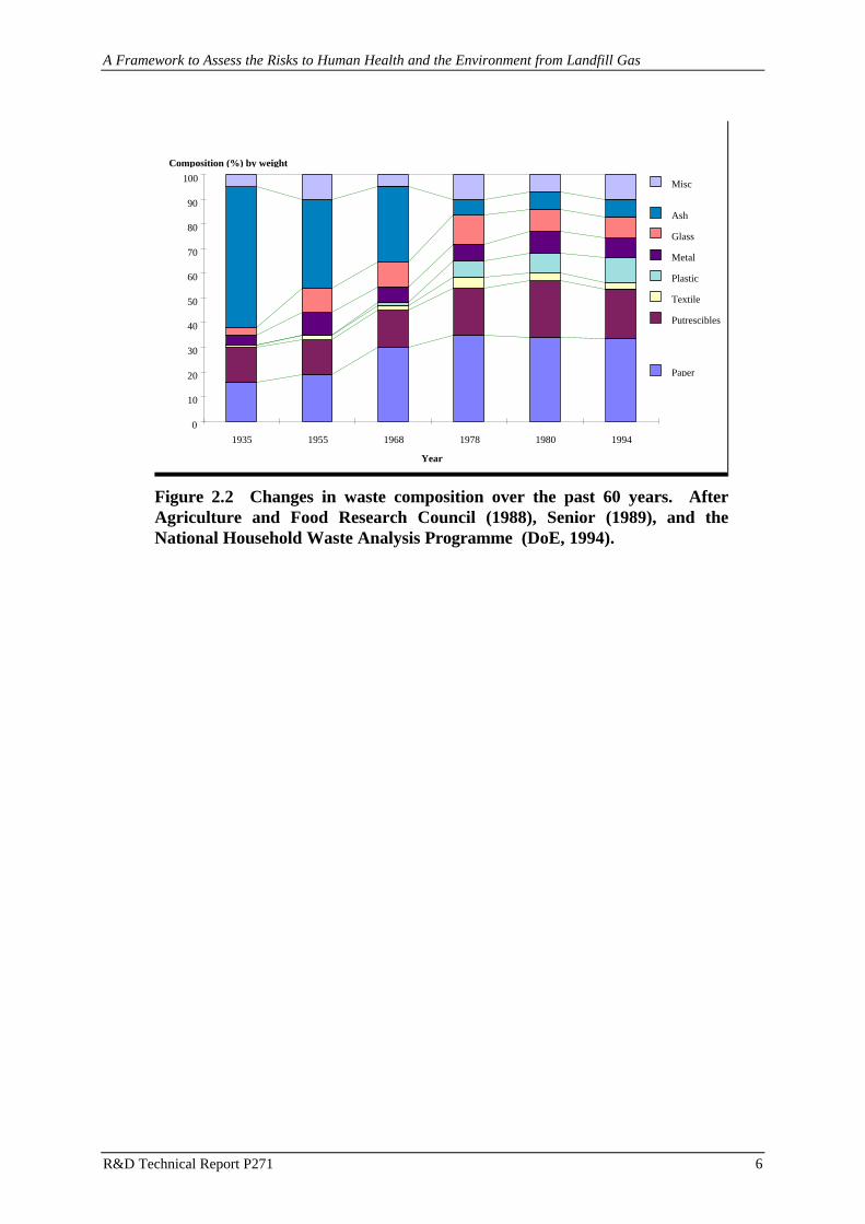
Again, most data are available for household waste compositions, and some waste streams(e.g. civic amenity wastes) would not have existed in certain eras. Figure 2.2 shows howhousehold waste composition has changed over the past 60 years. These data are included inthe source term module.
A Framework to Assess the Risks to Human Health and the Environment from Landfill Gas
R&D Technical Report P271 6
0
10
20
30
40
50
60
70
80
90
100
1935 1955 1968 1978 1980 1994
Year
Composition (%) by weight
Misc
Ash
Glass
Metal
Plastic
Textile
Putrescibles
Paper
Figure 2.2 Changes in waste composition over the past 60 years. AfterAgriculture and Food Research Council (1988), Senior (1989), and theNational Household Waste Analysis Programme (DoE, 1994).

A Framework to Assess the Risks to Human Health and the Environment from Landfill Gas
R&D Technical Report P271 7
2.3 Source term modelling
The timeframes in which LFG emissions and leachate formation are important in environmentalrisk assessment modelling are quite different, and the nature of the source terms are quitedifferent. Simulation of leachate loss from a landfill, using for example the leachate riskassessment model LANDSIM, is relatively straightforward. The assumption can be made thatthe source term (or the material which gives rise to the leachate), once determined, is non-variant with time (although a time-dependent source term is also available in LANDSIM forparticular modelling circumstances). The same is not true for LFG. The amount of gasgeneration for any particular landfill in any particular year varies significantly with, inter alia:
• the age of the site;• the nature of the waste deposited in the site;• the quantity of waste deposited; and• the hydrological, physical, chemical and biochemical regimes within the site.
The rate at which gas is generated within a site can vary significantly from year to year,particularly in the early phases of a sites’ gas generation lifespan, and the period over whichgas generation is an important consideration is much less than the time frames considered forleachate formation.
As a consequence, the approach adopted in this LFG risk assessment model is somewhatdifferent to that found in LANDSIM. The LFG source term model was developed initially as astand alone deterministic model. By this we mean a model which does not operate in aprobabilistic fashion, but which generates for the user ‘best estimates’ of LFG production andemission over the period of filling for the different waste compositions supplied to the model.
The modelling steps considered in the deterministic model are as follows:
1. Input waste composition as primary user input data on a yearly basis.2. Input waste quantities deposited in the landfill as primary user input data on a yearly basis.3. Input user defined information on the usage of LFG flares, and gas utilisation schemes; and
cap and liner designs, on a yearly basis.4. Calculate bulk gas generation on a yearly basis;5. Calculate trace gas and volatile organic compounds (VOC) generation on a yearly basis;6. Pass the bulk gas and trace gas/VOC generation rates to an output file/matrix for plotting.
The user has the option to stop at this stage, in order to:
• reassess the data used in the simulation; or• run the simulation again, using different gas management options, cap designs, etc.
This deterministic emissions model (DEMI) was a development stage on the route to the morecomplex HELGA model, but the flexibility of the source term module in DEMI made itappropriate to calculate some of the parameters required for the probabilistic HELGA model.These parameters were the ranges in waste composition available for degradation and thesubsequent degradation rates.

A Framework to Assess the Risks to Human Health and the Environment from Landfill Gas
R&D Technical Report P271 8
2.4 Selection of pollutants to be modelled
LFG comprises a complex cocktail of many gases and VOCs. There is no single compositionthat is appropriate to all sites. Rather, ranges of concentrations of any particular componentwithin the gas will be observed between usually well observed and defined limits. The gasesproduced will also depend to a certain extent upon the nature of the feedstock.
In selecting gases and VOCs to simulate in the model, we have had to split the method ofrepresentation in the model into two:
1. Those gases, for which mechanistic pathways have been identified, may comprise asignificant proportion of the gas generated, and whose particular temporal behaviour isreasonably well understood.
2. Those gases and VOCs for which mechanistic pathways may or may not have beenidentified, but whose temporal behaviour is not well understood.
Conveniently, gases that fall into group 1 above are produced in sufficient quantities to beconsidered as bulk components of LFG. Those which fall into group 2 above are found inLFG at much lower (but much more variable and therefore less predictable) concentrations.Group 1 gases are modelled in a different fashion to group 2 gases and VOCs, because of theconcentrations at which they occur in LFG.
2.4.1 Bulk gases
The following bulk gases are represented in the model:
• methane• carbon dioxide; and• hydrogen.
Methane and carbon dioxide together represent typically more than 95% of the gas generatedby the decomposition of the waste in the landfill. Methane is flammable, and poses a fire andexplosion hazard to neighbouring property. Laterally migrating methane can also beresponsible for displacing or removing oxygen from the root zone of vegetation, causingvegetation stress.
Carbon dioxide build up in properties can have an asphyxiant or other physiological affect onthe human body at relatively low concentrations, when compared to that found in LFG.Laterally migrating carbon dioxide can also be responsible for displacing or removing oxygenfrom the root zone of vegetation, causing vegetation stress. Both gases have a global climateeffect, although only methane, because of its high global warming potential relative to carbondioxide, is considered in the UK inventories of greenhouse gases.
Hydrogen is represented in the model, as it is produced primarily in the early acetogenic phaseof gas production, and although produced in lesser quantities than methane, has a lowerexplosive limit (LEL) than methane.
A Framework to Assess the Risks to Human Health and the Environment from Landfill Gas
R&D Technical Report P271 9
Combustion of methane and hydrogen in flares or gas utilisation plant convert a proportion ofthe methane to carbon dioxide, and hydrogen to water. Thus the result of running differentsimulations, with or without active gas control, will be a quantitative measure of the riskreduction for particular components of the LFG for certain pathways, and a quantitativemeasure of the increased risk from other components in the system. The user will have tomake a decision, based on the tolerability of risk, as well as on other considerations, as towhich management option is the most favourable.
2.4.2 Trace gases and VOCs
There are scant data available on the rate of production of trace gases and VOCs from landfills.The production of these species is conceptually linked to the rate of production of bulk gases.Thus, the rate of decomposition of materials in the waste which evolve the bulk gases is usedto similarly evolve trace gases and VOCs at rates proportional to the rate of bulk gasproduction.
Trace gases and VOCs in the model’s database have been selected for their potentialcontribution to human health and environmental effects. Other trace gases and VOCs may beadded on an ad hoc basis once the model has been completed, as data become available. Not alltrace gases or VOCs will be emitted from each gas emissions pathway, as some are emitteddirectly from the landfill surface, as components of the LFG, and others will be products ofcombustion or incomplete combustion of LFG from flares or utilisation plant. The emissionpathways, and the key trace gases/VOCs for each emission pathway, are shown in the sectionsbelow.
2.4.3 Surface emissions
The following components were included in the surface emissions model.
• Benzene and vinyl chloride, for their carcinogenic properties.• Trichloroethene and tetrachloroethene, as representative chlorinated solvents, for their
health effects.• Dioxin and furans for their health effects.• Carbon monoxide for its toxicity effects.• Chlorodifluoromethane and dichlorodifluoromethane for their global climate effects.• Hydrogen sulphide and methanethiol for their odour effects, as well as the toxicity of
hydrogen sulphide.• PM10.
Chemical conversion or degradation of any of these species during surface emission andsubsequent atmospheric transport was not considered.
2.4.4 Lateral emissions
The following trace components were included in the lateral emissions model:
A Framework to Assess the Risks to Human Health and the Environment from Landfill Gas
R&D Technical Report P271 10
• All components, except PM10, considered for surface emissions.
Chemical conversion or degradation of any of these species during lateral migration was notconsidered.
2.4.5 Flare emissions
The following components were included in the flare emissions pathway:
• All components considered for surface emissions. Conversion to other species in the flarereduced the proportion of many of these components for this pathway. The proportion ofsome components, e.g. PM10, may increase.
• Additional emissions of nitrogen oxides (NOx), sulphur oxides (SOx), hydrogen chloride,hydrogen fluoride, and carbon monoxide as specific flare emission products.
Chemical conversion or degradation of any of these species during subsequent atmospherictransport was not considered.
2.4.6 Utilisation plant emissions
This pathway considered emissions for a gas engine used for power generation, rather thandirect use of the gas, as this is the most common use for landfill gas at the present time. Thefollowing components were included in the utilisation plant emissions pathway:
• All components considered for surface emissions. Conversion to other species in theutilisation plant reduced the proportion of many of these components for this pathway. Theproportion of some components may increase.
• Additional emissions of nitrogen oxides (NOx), sulphur oxides (SOx), hydrogen chloride,hydrogen fluoride, PM10, and carbon monoxide as specific engine exhaust emissionproducts.
Chemical conversion or degradation of any of these species during subsequent atmospherictransport was not considered.
2.4.7 Odour
A special case is the consideration of odour. Two gases are represented in the model forodour emissions from the surface of landfills: hydrogen sulphide and methanethiol. Theirodour properties will be significant reduced via the lateral migration pathway due to sorptionprocesses, or via flares or utilisation plant, due to destruction in the combustion process.
2.5 Pathways and targets
The pathways considered in the environmental transport module are:
A Framework to Assess the Risks to Human Health and the Environment from Landfill Gas
R&D Technical Report P271 11
• atmospheric dispersion off-site;• atmospheric dispersion on-site; and• lateral migration through the ground.
Atmospheric dispersion off-site is considered for pollutant emissions from the landfill cap,landfill gas flares and gas utilisation plant. Dispersion on-site is relevant to the estimation ofrisks to landfill workers. In this instance all surface emissions are considered.
For lateral migration of gases through the ground a distinction has been made between a steadystate situation and unusual conditions. For the steady state case annual average emissions fromthe landfill boundary will be used as input to the migration model. The unusual conditions partof the module simulates the sorts of situations in which emission and migration rates increasewell above the annual average for a brief period. The occurrence of such a condition has beentreated as a probabilistic event.
The exposure assessment module has two major functions:
• the calculation of concentrations of pollutants in indoor air, as a result of atmosphericdispersion and lateral migration; and
• the calculation of intakes of pollutants by humans.
In the latter case both members of the public and workers are considered but the emphasis ison members of the public. The main exposure pathways included for members of the publicare inhalation, ingestion of home-grown vegetables and dermal exposure. For workersinhalation and dermal exposure are considered.
The impact assessment module estimates risks to human health, using output from theexposure assessment module. It also estimates local and global environmental impacts usingoutput from the source term and environmental transport modules. Vegetation stress is thelocal impact considered, while global impacts are greenhouse gases and ozone depletors.
2.6 Probabilistic aspects
Many of the data that drive the model have a wide margin of uncertainty. This could lead tolarge uncertainties in the outputs, particularly in the landfill gas generation module. It was arequirement for the project that the probabilistic approach in the gas risk assessment modelshould be consistent with that in LANDSIM. The intention was to couple the MicrosoftExcel™ spreadsheet package to Microsoft Crystal Ball™, which allows probability densityfunctions (pdfs) to be attributed to certain parameters which have a high uncertainty. Thisapproach was not adopted in the final version of HELGA for the following reasons:
• pdfs would have been required for a large number of user specified and model suppliedparameters;
• Crystal Ball™ can only work satisfactorily with a smaller number of probabilistic variablesthan would have been required in the model;
A Framework to Assess the Risks to Human Health and the Environment from Landfill Gas
R&D Technical Report P271 12
• the coupled Excel™/Crystal Ball™ model would have run at an unacceptably slow rate formodel users; and
• not all Environment Agency users would have had access to the Crystal Ball™ software,whereas all had access to Excel™.
With these considerations in mind, a pseudo-probabilistic approach to the model was devised.The HELGA model now represents uncertainty by using look-up tables generated by samplingparameter values from probability distributions for the source term (gas generation andemission) module. The software used to generate these look-up tables was Crystal Ball™, butthere is now no reliance on Crystal Ball™ when using HELGA.
Outputs from the Crystal Ball™ simulations were pdfs of landfill gas generation. From these,the mean, 95th percentile and 5th percentile values of landfill gas generation were derived.These were imported into HELGA as look-up tables calibrated per tonne of waste per year,which could then be scaled up to individual site tonnages. Landfill gas generation is thenpredicted as the mean, 95th percentile and 5th percentile values for subsequent use in theemissions, atmospheric dispersion, exposure assessment and impact assessment modules. Thedata on VOC and trace gas concentrations in landfill gas are used directly to calculate theproportion of trace gases released via each emission pathway. No chemical reactions arerepresented in the model which could convert trace gases to other chemical species, althoughthe emissions pathways (lateral migration, cap, flare or gas utilisation) consider differentcomponents characteristic of those pathways, and methane oxidation is permitted in thecapping layers.
The atmospheric dispersion part of the environmental transport model is probabilistic in thesense that it produces primarily annual average concentrations of pollutants in air, taking intoaccount the probabilities of occurrence of various weather conditions during a year.
The exposure assessment module is deterministic, because the people and buildings consideredare notional, and the parameters which characterise them are not subject to the same kind ofuncertainty as those in the source term and environmental transport modules (where the valuesof all the parameters are, in principle, measurable). The impact assessment module is alsodeterministic, because detailed consideration of uncertainties in parameter values for thevarious parts of this module is beyond the scope of this project.
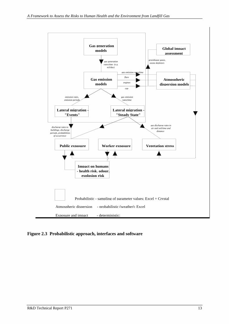
Figure 2.3 summarises the probabilistic and deterministic aspects of the model.
A Framework to Assess the Risks to Human Health and the Environment from Landfill Gas
R&D Technical Report P271 13
Gas generationmodels
Gas emissionmodels
Global impactassessment
Lateral migration -"Steady State"
Lateral migration -"Events"
Worker exposurePublic exposure Vegetation stress
Impact on humans- health risk, odour,
explosion risk
Atmosphericdispersion models
gas generationrates/time (e.g.
m3/day)
greenhouse gases,ozone depletors
gas emission rates/time
flare
cap
engines
emission rates,emission periods
gas emissionrates/time
discharge rates tobuildings, dischargeperiods, probabilities
of occurrence
gas discharge rates toair and soil/time and
distance
Probabilistic - sampling of parameter values; Excel + Crystal
Exposure and impact - deterministic;
Atmospheric dispersion - probabilistic (weather); Excel
Figure 2.3 Probabilistic approach, interfaces and software

A Framework to Assess the Risks to Human Health and the Environment from Landfill Gas
R&D Technical Report P271 14
3. SOURCE TERM
The emission rate of LFG from the landfill site is the source term for the risk assessment model(see Figure 2.1). The source term module is the critical component of the overall riskassessment model because the risk from LFG is proportional to its release from the site.
The generation rate and total yield of LFG are landfill site specific. LFG generation dependson the waste mix1 and composition2 and the environmental conditions in which the wastedegrades. All these factors differ from site to site. Additionally LFG generation andcomposition at any site change with time. The actual production and flux of gas from aparticular site at a particular time can only be ascertained by lengthy and comprehensive directmeasurement.
Mathematical modelling provides an approximation of LFG processes and so is useful toestimate LFG generation when comprehensive site measurements are not available. This isusually the case. In particular LFG generation models are necessary to make projections ofLFG generation and emissions.
3.1 Landfill gas generation
The are several methods for modelling LFG generation. Most are based on a description ofLFG formation based on laboratory experiments or full-scale field measurements. The modelsrange from relatively simple zero-order (time-independent) equations through first-order modelthat have a decay function to more complex second-order equations that try to model a numberof different reactions taking place at different rates.
Oonk et al. (1994) validated a number of LFG models using data from gas recovery schemes.They concluded that the description of LFG formation improves going from a zero-ordermodel, to a first- and second-order model. However a variant on the single-order model, amulti-phase model, provided the best correlation with field results (see Section 3.1.1.2).
All LFG models produce uncertain results. This uncertainty derives from the heterogeneity ofboth landfilled waste and the conditions under which it degrades, and the limited availability ofinformation and data to put into models. Any new LFG model should aim to reduce theseuncertainties whilst allowing for limits in input data. We have developed a new multi-phaseLFG generation model. It is based on the model developed originally by Hoeks and Oosthoek(1981) and described by van Zanten and Scheepers (1996). The model is a significantdevelopment on previous models because it can:
• define precisely the mix, composition and moisture content of waste in the landfill site;and
• calculate LFG generation based on the degradation rates of the individual materials inthe landfilled waste.
1 The proportion of different types of waste, e.g. household, commercial, industrial, in the landfilled waste.2 The specific materials, e.g., newspaper, food waste, cardboard, textiles, in each type of waste in the mix.

A Framework to Assess the Risks to Human Health and the Environment from Landfill Gas
R&D Technical Report P271 15
These additions make the model highly flexible. It can be tailored to individual landfill sites,taking account of specific waste streams, filling rates and environmental conditions. As withall LFG models, the accuracy of this module is limited by the availability of input data. Themore site specific information there is, the more certain the module outputs will be. However,if there is limited input data, the module has default parameters that can be chosen by the user.This allows the module to approximate LFG generation using the user’s best knowledge ofany landfill site.
3.1.1 Module description
There are two main processes in the module:
1. Defining the waste in the landfill site; and2. Calculating LFG generation from a specified mass of waste.
3.1.1.1 Defining the waste
The rate of generation and total yield of LFG depends on the mix and composition of wastedisposed in the landfill site. The main source of carbon in LFG is from the degradation ofcellulose and hemi-cellulose. Different biodegradable materials in the waste have differentproportions of cellulose and hemi-cellulose. The ultimate degradability of the cellulosepolymers also differs between waste materials. Thus the total yield of LFG and its rate ofproduction depend on the mass and degradability of the cellulose and hemi-cellulose in thewaste.
This module is highly flexible because it can accommodate any combination of waste types,mix and composition This allows the user to customize the module according to the waste inplace or that projected for individual sites.
In all cases the user will choose the proportion of different waste types in the total mix.
The user can also define the composition of each waste in the mix. If the waste composition isnot known then an approximation can be chosen. To help with this, the module at presentcontains three pre-selected waste types:
Waste 1 Typical composition of waste during the period 1956 -1976;Waste 2 Typical composition of waste during the period 1976 to the present
date;Waste 3 Future Landfill Directive waste composition1; andWaste 4 User defined (may also cover wastes prior to 1956).
Table 3.1 shows the composition of degradable components in Waste 2. Each waste type alsocontains inputs for the non-biodegradable, or inert, components of the mix (not shown in Table3.1). The composition of Waste 2 is typical of contemporary waste. The proportion of
1 This is a projected waste stream make up, that will take into account the proposed directives on the landfillingof wastes.

A Framework to Assess the Risks to Human Health and the Environment from Landfill Gas
R&D Technical Report P271 16
different materials in the domestic waste and the cellulose/hemi-cellulose content are from theNational Household Waste Analysis Project (DoE, 1994). The percentage degradability isfrom Barlaz et al. (1996).
Although provided in the module, the user can alter all the parameters such as composition,water content, cellulose and hemi-cellulose content and percentage degradation if better oralternative information is available.

R&D Technical Report P271 17
Table 3.1 Composition of waste components in a contemporary waste mix
1980's - 1997FRACTIONDegradable Domestic Civic
AmenityCommercial Industrial Inert Liquid
InertSewagesludge
Watercontent
(%)
Cellulose(%)
Hemi-cellulose
(%)
Decomposition(%)
Paper/CardNewspapers 11.38 10 10 30 48.5 9 35Magazines 4.87 11 30 42.3 9.4 46Other paper 10.07 50.1 30 87.4 8.4 98Liquid cartons 0.51 30 57.3 9.9 64Card Packaging 3.84 30 57.3 9.9 64Other card 2.83 30 57.3 9.9 64
TextilesTextiles 2.36 3 25 20 20 50
Miscellaneouscombustible Disposable
nappies4.35 20 25 25 50
Other misc.combustibles
3.6 20 25 25 50
PutrescibleGarden waste 2.41 22 65 25.7 13 62Otherputrescible
18.38 15 65 55.4 7.2 76
Fines10mm fines 7.11 15 40 25 25 50
Sewage sludgeSewage sludge 100 70 14 14 75
A Framework to Assess the Risks to Human Health and the Environment from Landfill Gas
R&D Technical Report P271 18
3.1.1.2 Calculating landfill gas generation
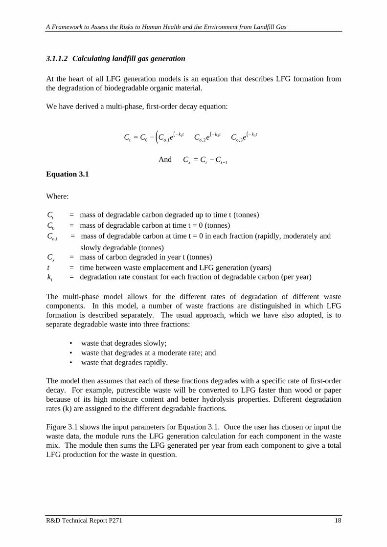
At the heart of all LFG generation models is an equation that describes LFG formation fromthe degradation of biodegradable organic material.
We have derived a multi-phase, first-order decay equation:
( ) ( ) ( )( )C C C e C e C et ok t
ok t
ok t= − + +− − −
0 1 2 31 2 3
, , ,
And C C Cx t t= − −1
Equation 3.1
Where:
Ct = mass of degradable carbon degraded up to time t (tonnes)C0 = mass of degradable carbon at time t = 0 (tonnes)Co i, = mass of degradable carbon at time t = 0 in each fraction (rapidly, moderately and
slowly degradable (tonnes)Cx = mass of carbon degraded in year t (tonnes)t = time between waste emplacement and LFG generation (years)ki = degradation rate constant for each fraction of degradable carbon (per year)
The multi-phase model allows for the different rates of degradation of different wastecomponents. In this model, a number of waste fractions are distinguished in which LFGformation is described separately. The usual approach, which we have also adopted, is toseparate degradable waste into three fractions:
• waste that degrades slowly;• waste that degrades at a moderate rate; and• waste that degrades rapidly.
The model then assumes that each of these fractions degrades with a specific rate of first-orderdecay. For example, putrescible waste will be converted to LFG faster than wood or paperbecause of its high moisture content and better hydrolysis properties. Different degradationrates (k) are assigned to the different degradable fractions.
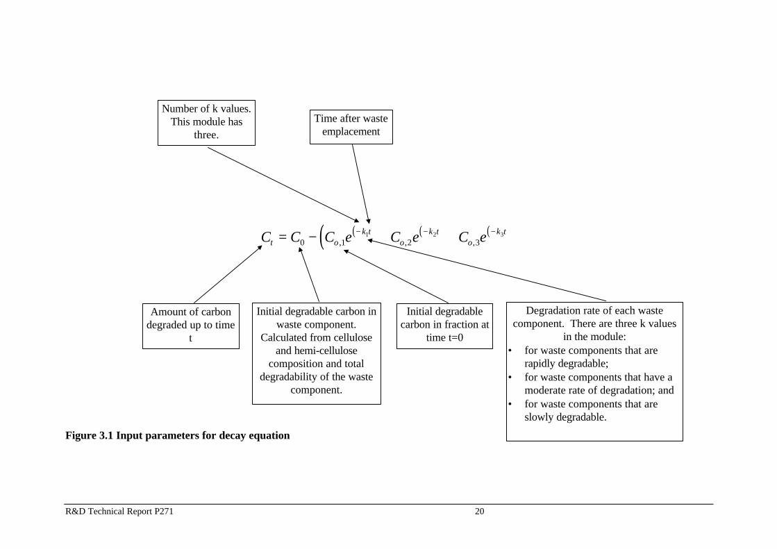
Figure 3.1 shows the input parameters for Equation 3.1. Once the user has chosen or input thewaste data, the module runs the LFG generation calculation for each component in the wastemix. The module then sums the LFG generated per year from each component to give a totalLFG production for the waste in question.

A Framework to Assess the Risks to Human Health and the Environment from Landfill Gas
R&D Technical Report P271 19
3.2 Using the source term module
The LFG source term model has been constructed in a modular form, that presents therequired inputs and outputs in a logical fashion to facilitate its use. The model is based aroundnine Excel work sheets (Figure 3.2):
• QA Sheet;• Input Sheet;• Wastes 1 - 4;• Wastes Water Content;• Defaults and Data; and• Data Manipulation.
The inputs, links, calculations and output of the worksheets are described in the followingsections.
R&D Technical Report P271 20
( ) ( ) ( )( )C C C e C e C et ok t
ok t
ok t= − + +− − −
0 1 2 31 2 3
, , ,
Figure 3.1 Input parameters for decay equation
Time after wasteemplacement
Number of k values.This module has
three.
Degradation rate of each wastecomponent. There are three k values
in the module:• for waste components that are
rapidly degradable;• for waste components that have a
moderate rate of degradation; and• for waste components that are
slowly degradable.
Initial degradable carbon inwaste component.
Calculated from celluloseand hemi-cellulose
composition and totaldegradability of the waste
component.
Initial degradablecarbon in fraction at
time t=0
Amount of carbondegraded up to time
t

A Framework to Assess the Risks to Human Health and the Environment from Landfill Gas
R&D Technical Report P271 21
3.2.1 QA sheet
The QA Sheet has been included to allow relevant project details to be entered and saved as anintegral part of each run. It is hoped that these details will be unique, allowing each run to betraceable to the relevant time, project and user. This sheet allows for the input of:
• project name;• project number;• site details (location and owner); and• site fill time details
The QA sheet as it stands is an initial pass and is expected to be modified once the rest of themodel has been constructed and validated. It is considered to be an important part of the finalmodel, and will be straight forward to develop once the model is more fully developed.
Details on the commencement of waste filling in the landfill site is linked into the Input Sheet,so that the specific date for each year of filling is presented.
3.2.2 Input sheet
The Input Sheet requires data input for the fill rate of the landfill site; included in this is thefacility to apportion the waste entering the site to different production streams (see Section2.2).
The user can input up to 50 years’ data on the volume of waste entering the site (50 years filltime is expected to be the maximum likely for a landfill, as agreed with the project steeringcommittee). The volumes of waste are converted to tonnage using an input density for thewaste, the default will be 1 tonne.m-3. The waste mass entering the site can be used, but thecalculation to convert from volume to tonnes will be overwritten.
The make up of the waste streams coming to the landfill is known to have changed over time,so the model has the flexibility to input four different waste stream make-ups. The fourdefined time periods will initially be:
• 1956 - 1976;• 1976 - present day;• Landfill Directive mix; and• user defined (may also include pre 1956 waste).
Most data available are for the period 1976 to present day.

R&D Technical Report P271 22
Project Details:Site
LocationOperation company
Etc.
Filling dates:Commencement
End
QA details:Signatures
General project description
QA SHEET
INPUT
INPUT
INPUT
Waste fractioncomposition:
(1) 1950's - 1970's(2) 1980's - 1997(3) 1998 - 2015(4) User defined
% Cellulose /Hemicellulose
% Moisture in freshwaste
% Degradability ofcellulose in each
fraction of the waste
WASTES (1-4)
INPUT
INPUT
Rain and other water infiltrationrates
to the site
WASTES WATERCONTEN
INPUT
INPUT
Waste hydraulic properties
Leachate conditionsin the landfill site
INPUT
K and T (1/2) for the differentdegradable carbon fractions:
(1) Rapidly(2) Moderately
(3) Slowly
DEFAULTS ANDDATA
INPUT
Waste voulume inputper year
Waste stream sourceareas
Waste sourcecomposition (1-4 dependant date of
filling + user definedwaste type)
INPUT
INPUT
INPUT
INPUT
% Each waste fraction depositedin site per year
Dry weight of waste fractions intosite per year (Mt) Total dry weight of
waste in site per year (Mt)
DATA MANIPULATION
Cellulose and hemicellulose contentof the waste (Mt)
Mass of degradablecarbon (Mt)
Mass of degradable carbon (Mt)(1) Rapidly degradable
(2) moderately degradable(3) Slowly degradable
Carbon degraded in wasteper year (Mt)
Cumulative carbon degraded in siteper year (Mt)
DATA MANIPULATION
LFG production in the landfill per
year: (m3), MethaneCarbon dioxide, Hydrogen
Cumulative LFG production in the landfill
each year after filling commences: (m3)Methane Carbon dioxide Hydrogen
EMISSIONSWORK BOOK
Degradability of each waste fractionINPUT
Methane to carbondioxide split in LFG
Figure 3.2 Source term model flow diagram
A Framework to Assess the Risks to Human Health and the Environment from Landfill Gas
R&D Technical Report P271 23
3.2.3 Wastes 1 - 4
The user inputs the waste stream mixes in each of these sheets. The waste streams aredisaggregated into a number of components, as designated in the National Household WasteAnalysis Programme (DoE, 1994), with two other components (soil and brick) to allow forbuilding wastes. Each of the sheets inputs are taken as the default of the waste streamcomposition for a specific time period to allow for temporal trends in the waste make-up.
Included on Waste 4 are the data on the cellulose and hemi-cellulose content of eachbiodegradable waste component and the degradability of the cellulose and hemi-cellulose.These compounds are known to make up about 91%, of the degradable fraction of refuse(Barlaz et al., 1989). Other potentially degradable fractions, e.g. protein and lipids, are notincluded here as they do not contribute significantly to LFG emissions (although they may be asource of pollutants in leachate).
The degradability of the waste is input at this point in the model, rather than later as seen on anumber of models (Oonk 1994). This allows greater flexibility in describing the wastesentering the site, and will allow for greater manipulation of the input data as further researchprovides more information.
The moisture content of each component is entered on the Waste 4 sheet. This allows the dryweight of the waste to be calculated on the Data Manipulation Sheets.
The cellulose and hemi-cellulose content of the waste components is linked to the DataManipulation Sheet, and is used to calculate the dry mass of each component in the waste forevery fill year.
3.2.4 Waste water content
The hydraulic and physical properties of the landfill are entered on this sheet in order todetermine the percentage saturation of the waste mass. These data are then used to select thedegradation rate constants of the slowly, moderately and rapidly degradable cellulose fractionsin the waste.
3.2.5 Defaults and data
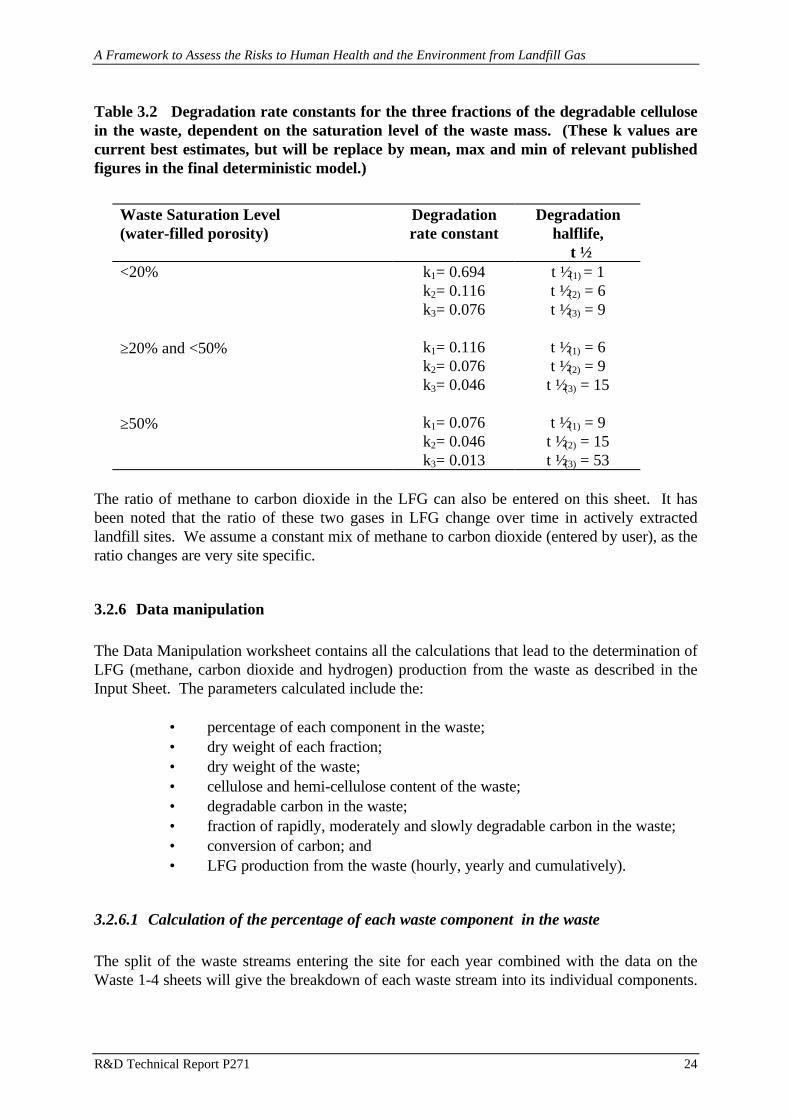
The degradation rate constants for each fraction of the cellulose/hemi-cellulose are related tothe level of saturation of the waste. This is known to have a significant effect on thedegradation rate. Therefore, we have linked the degradation rate constants for each of thethree cellulose fractions to the waste saturation level (Table 3.2).
A Framework to Assess the Risks to Human Health and the Environment from Landfill Gas
R&D Technical Report P271 24
The ratio of methane to carbon dioxide in the LFG can also be entered on this sheet. It hasbeen noted that the ratio of these two gases in LFG change over time in actively extractedlandfill sites. We assume a constant mix of methane to carbon dioxide (entered by user), as theratio changes are very site specific.
3.2.6 Data manipulation
The Data Manipulation worksheet contains all the calculations that lead to the determination ofLFG (methane, carbon dioxide and hydrogen) production from the waste as described in theInput Sheet. The parameters calculated include the:
• percentage of each component in the waste;• dry weight of each fraction;• dry weight of the waste;• cellulose and hemi-cellulose content of the waste;• degradable carbon in the waste;• fraction of rapidly, moderately and slowly degradable carbon in the waste;• conversion of carbon; and• LFG production from the waste (hourly, yearly and cumulatively).
3.2.6.1 Calculation of the percentage of each waste component in the waste
The split of the waste streams entering the site for each year combined with the data on theWaste 1-4 sheets will give the breakdown of each waste stream into its individual components.
Table 3.2 Degradation rate constants for the three fractions of the degradable cellulosein the waste, dependent on the saturation level of the waste mass. (These k values arecurrent best estimates, but will be replace by mean, max and min of relevant publishedfigures in the final deterministic model.)
Waste Saturation Level(water-filled porosity)
Degradationrate constant
Degradationhalflife,
t ½<20% k1= 0.694
k2= 0.116k3= 0.076
t ½ (1) = 1t ½ (2) = 6t ½ (3) = 9
≥20% and <50% k1= 0.116k2= 0.076k3= 0.046
t ½ (1) = 6t ½ (2) = 9
t ½ (3) = 15
≥50% k1= 0.076k2= 0.046k3= 0.013
t ½ (1) = 9t ½ (2) = 15t ½ (3) = 53
A Framework to Assess the Risks to Human Health and the Environment from Landfill Gas
R&D Technical Report P271 25
Using this information, the percentage wet weight of each component in the waste depositedper year can be determined.
3.2.6.2 Calculation of the dry weight of each fraction in the waste
Using the waste percentage composition of the various components and the moisture contentof each waste fraction entered on Waste (4) sheet, the dry weight of the components and thetotal waste deposited yearly can be calculated.
Details on the moisture content of various waste fractions are only available in general terms,and therefore these can be defined if more reliable data are available for specific wastefractions.
3.2.6.3 Calculation of the cellulose and hemi-cellulose content of the waste
The cellulose and hemi-cellulose content of each waste fraction are provided along with themoisture content in Waste (4) sheet. Therefore the cellulose/hemi-cellulose content of thewaste input can be determined for each year. Waste (4) sheet also accepts the degradability ofthe cellulose and hemi-cellulose fractions in the waste, and thus the degradable cellulose andhemi-cellulose mass can be calculated. This is then sub-divided into three fractions:
• rapidly degradable;• moderately degradable; and• slowly degradable.
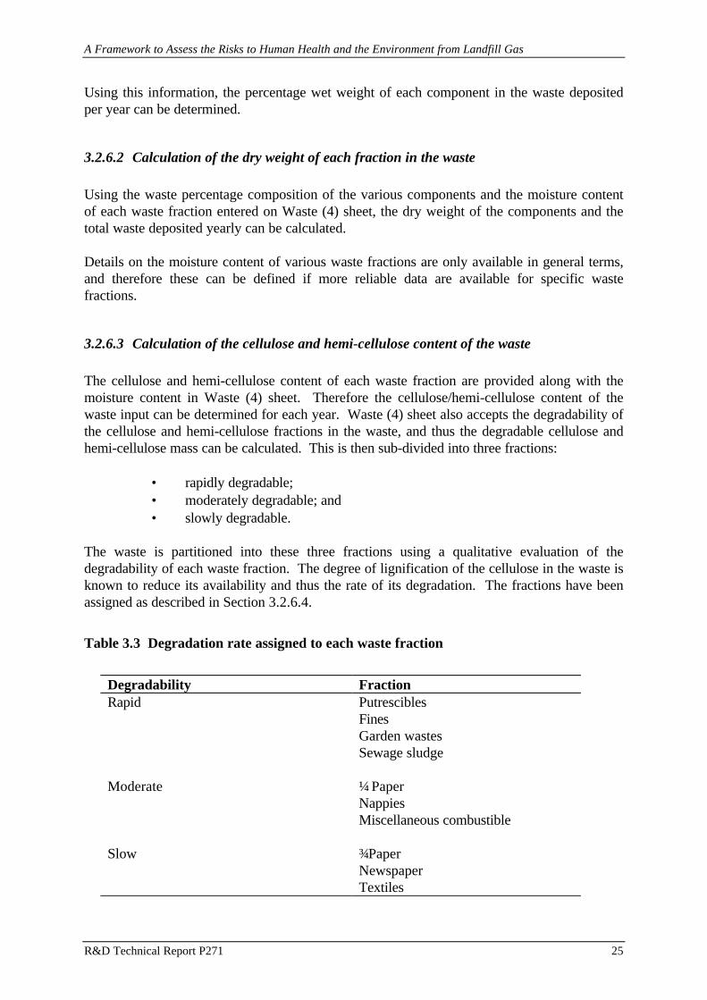
The waste is partitioned into these three fractions using a qualitative evaluation of thedegradability of each waste fraction. The degree of lignification of the cellulose in the waste isknown to reduce its availability and thus the rate of its degradation. The fractions have beenassigned as described in Section 3.2.6.4.
Table 3.3 Degradation rate assigned to each waste fraction
Degradability FractionRapid Putrescibles
FinesGarden wastesSewage sludge
Moderate ¼ PaperNappiesMiscellaneous combustible
Slow ¾ PaperNewspaperTextiles

A Framework to Assess the Risks to Human Health and the Environment from Landfill Gas
R&D Technical Report P271 26
To allow for the inclusion of hydrogen in the model, a percentage of the rapidly degradablefraction of the waste is assumed to be degraded acetogenically, with the formation of acetate,carbon dioxide and hydrogen (no methanogenesis occurs in the newly deposited anaerobicwaste, so the hydrogen and carbon dioxide are free to be produced and not converted tomethane). This is assumed to occur only in the first year after waste is deposited, then thedegradation follows the methanogenic pathway. The percentage of the waste degraded by thispathway may be entered, but we have set the default at 1%, as this gives a maximumconcentration of hydrogen in LFG of around 10%. This fits our understanding of landfillprocesses, including the pioneering work of Farquhar and Rovers (1973). The inclusion ofhydrogen will allow us to initially evaluate the risk it presents, with the result that it mayeventually be removed, depending on the results of the scoping work.
3.2.6.5 Degradation of the degradable carbon compounds
Degradation of the degradable carbon compounds in the waste is described by a first-order,multiphase equation where each of the three degradable fractions are dealt with separately andthe resultant amount of carbon converted to LFG per year is aggregated. The degradation rateconstants used in the equation are taken from published data, and derived from the wastesaturation levels, as detailed above.
3.2.7 LFG production
Once the carbon available to be converted per year has been calculated, the volume ofmethane, carbon dioxide and hydrogen can be determined. The ratio of methane to carbondioxide in the LFG, is entered on the Defaults and Data sheet and 1 mole of carbon produces 1mole of methane or carbon dioxide. The conversion of carbon to an equivalent of hydrogen isgiven by Equation 3.2. From this the total LFG production, both hourly and cumulative can beevaluated.
The results produced in this sheet are then copied to the emissions model. Having the twomodels running in series, reduced the size of a single Excel file and thus the run time for anymanipulations.
3.2.6.4 Biodegradation
The degradable cellulose and hemi-cellulose in the waste are converted to degradable carboncompounds. It is assumed that the anaerobic degradation is generally methanogenic, with theratio of methane to carbon dioxide specified in the Defaults and Data sheets.
C H O C H C O O H H C O
or C e llulose Acet ic Ac id H y d r o g e n C a r b o n D ioxide
or C a r b o n Acet ic Ac id H y d r o g e n C a r b o n D ioxide
Ace togenes is
Ace togenes is
6 12 6 3 2 22 4 2
6 2 4 2
→ + +
→ + += + +
Equation 3.2 Production of hydrogen from the degradation of cellulose

A Framework to Assess the Risks to Human Health and the Environment from Landfill Gas
R&D Technical Report P271 27
3.3 Landfill gas emissions
The LFG generation details are copied from the generation model (both have to be open to dothis) using a macro that is activated using <Ctrl + d>. This pastes data from the generationmodel into the LFG Data sheet, where it is then used in emission calculations.
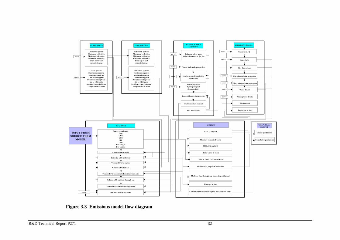
The emissions model is based around six work sheets (Figure 3.3):
• LFG Data;• Flare Input;• Utilisation;• Waste Water Content;• Emissions Route; and• Output.
There are currently two graphical outputs. One presents a yearly averaged hourly emissionfrom the site to the different routes over the assessment period (user defined) and the othergives the cumulative emissions. The carbon is degraded for a period of 300 years as thisperiod will result in the degradation of the majority of the carbon, the period of interestgenerally may only be 100 years, but it gives the flexibility to look over longer time frames.The pathways considered are:
• utilisation (energy recovery);• flare; and• uncontrolled emissions (cap and liner).
3.3.1 Landfill gas data
The LFG Data sheet is used in the calculation of the emissions from the site for the wholeassessment period (300 years). As detailed above data from the Data Manipulation sheet ofthe source term model are copied onto this sheet and, then manipulated to give:
• volume of LFG to engine;• volume of LFG to flare;• volume of LFG lost in uncontrolled emissions;
∗ volume through the cap∗ volume through the liner
• methane oxidation in the cap.
3.3.1.1 Landfill collection
The LFG collection system has been specified to have a maximum and minimum capacity, andcan be specified to commence operation after a fixed time period or when the LFG productionis high enough to allow it to work (as detailed above).

A Framework to Assess the Risks to Human Health and the Environment from Landfill Gas
R&D Technical Report P271 28
It is assumed that if any gas is collected and not utilised in any manner (flared or used forenergy recovery) then that gas is assumed to be emitted through the cap and liner.
The collection system is assumed to have an envelope of operation, and if the gas production inthe site is less than the maximum capacity, then its operation is taken to be trimmed to followthe gas production curve (in reality it is trimmed to the point just before air is pulled into thesite).
The input of a collection efficiency allows the gas collection system to be less than 100%effective. Therefore when all the gas is being collected and utilised there will still be someLFG emissions from the site. This has been shown by other workers (Oonk et al., 1994), andsuch emissions are observed in practice (WS Atkins, 1997).
3.3.1.2 Volume of landfill gas to energy recovery plant
The routing of LFG to an energy recovery plant (utilisation) is either dependent on the time asspecified in the Utilisation sheet or linked to the LFG production rate. If the production rate ofgas is below the units utilisation volume, as specified in the Utilisation sheet, it is deemedinoperative, and the gas collected is either flared or emitted from the site.
3.3.1.4 Uncontrolled emissions from the site
Uncontrolled emissions from the site are split into two emissions routes, cap and liner. Bothare based on a steady state system where QRES (residual gas production) is equal to theemissions from the site (Equation 3.3). This QRES results in a slight excess pressure in the site(Pw) (Equation 3.4), compared to the atmosphere and can be used to calculate QSTORAGE (gasstored in landfill site). The storage capacity is slightly higher than that determined from solelythe pore volume.
3.3.1.3 Volume of landfill gas to flare
As with the collection system the flare has a maximum and minimum operational rate, and thisis usually scoped to deal with all the LFG collected. A flare system can be specified for the siteor not. If no flare is specified then it will be omitted from any of the calculations and assumedthat the gas collection system is being controlled solely on the engine capacity. If a flare isspecified then it will operate if the collection system is in operation and the gas available isgreater than its minimum requirement.
A Framework to Assess the Risks to Human Health and the Environment from Landfill Gas
R&D Technical Report P271 29
Emissions from the cap or liner are regulated by the permeability and thickness of the mostimpervious layer. Therefore this data is taken from the Emissions sheet where the thicknessand permeability of the emissions regulating layer have been determined. If the waste is themost impervious layer then its thickness is assumed to be half the average waste thickness.
Qres = Qgen - (Qflare + Qutilisation)
Where:Qgen LFG generated in the landfillQflare LFG routed to flare systemQutilisation LFG routed to the energy recovery plant
Equation 3.3
For a homogeneous medium Darcy’s law gives:
( )Q
K P P
P dw s
g
=−* 2 2
02µ
Equation 3.4
Where:Q gas volume flux (volume at pressure P0) to surface
K* effective permeability of medium (taking into account any waterpresent)
Pw pressure in waste (not a function of depth in this formulation)Ps pressure at surfaceP0 standard pressureµ g gas viscosity
d thickness of medium in direction of flow
A Framework to Assess the Risks to Human Health and the Environment from Landfill Gas
R&D Technical Report P271 30
Emissions from the cap and liner can then be calculated using Equation 3.5.
This pressure can be used in the simulation of an ‘event’, where the atmospheric conditionschange radically, for example a rapid decrease in atmospheric pressure. The differencebetween the atmospheric pressure and the landfill will be the driving force for such a migrationevent
3.3.1.5 Methane oxidation
Methane oxidation in the cap of landfills is well known (DoE 1991; DoE 1994a), but the extentto which it occurs is related to the cap type, thickness and the LFG flux. This model has twodefaults for methane oxidation in the cap that are related to the residence time of the LFG as itpasses out of the site. The residence time is related to the cap thickness and the emissions ratefrom the cap. The model assumes 50% methane oxidation for thick caps with low emissions orhigh residence times. The model assumes 10% for thin caps and high emission rates or shortresidence times. This part of the model needs further development, but we have included itnow to show how it is to be integrated into the whole framework.
3.3.2 Flare Input
The Flare Input sheet allows data on the operational capabilities of the LFG collection andflare systems to be entered.
3.3.2.1 Collection system
The LFG collection system is assigned a maximum and minimum extraction capacity, acommissioning time after waste tipping commences and a collection efficiency. The collectionsystem, for the sake of this model, follows the gas production trend from its commissioninguntil it reaches the maximum capacity of the flare specified. Then gas produced is lost byuncontrolled emission. When the LFG production rate drops below the minimum operational
d
K
K
d
cres
c
c
l
l
=
+. 1
d
K
K
d
lres
l
l
c
c
=
+. 1
Equation 3.5
Where:Qc Flux from cap (l = liner)
the rest are as previously stated
A Framework to Assess the Risks to Human Health and the Environment from Landfill Gas
R&D Technical Report P271 31
level of the flare system, the flare is switched off, and LFG is then emitted from the site eitherthrough the liner or cap.
3.3.2.2 Flare system
The flare can be switched off or on, and it is assigned a maximum and minimum capacity. It isassumed to be operational when the collection system has been commissioned (dependent onthe expected commissioning date entered). The flare is assumed to be running if the collectionsystem is in service and the LFG available is sufficient for flaring, i.e. greater than its minimumoperational needs. The flare can be used in conjunction with the utilisation plant, when it cancollect any excess gas that is not used for energy recovery.
Details on the flame temperature and residence time in the flare are also input for use in theemissions model. This section of the model has not yet been developed.
R&D Technical Report P271 32
Source term input:DateCH4CO2H2
LFGWet weightDry weight
Potential LFG collected
Volume LFG to engine
LFG DATA
INPUT FROM SOURCE TERM
MODEL
INPUT
Collection efficiency
Volume LFG uncontrolled emittion from site
Volume LFG to flare
Volume LFG emitted through liner
Volume LFG emitted through cap
Methane oxidation in cap
FLARE INPUT
Collection system:Maximum collection Minimum collectionCollection efficiency
Years up to unit commissioning
Flare system:Maximum capacityMinimum capacityComissioning year
De-comissioning YearAir to LFG ratio
Residence time in flameTemperature of flame
UTILISATION
Collection system:Maximum collection Minimum collectionCollection efficiency
Years up to unit commissioning
Utilisation system:Maximum capacityMinimum capacityComissioning year
De-comissioning YearAir to LFG ratio
Residence time in engineTemperature of burn
INPUT
INPUT
Rain and other water infiltration rates to the site
WASTES WATER CONTENT
Waste hydraulic properties
Leachate conditions in the landfill site
Waste physical/ hydrogeological characteristics
Free void space in the waste
Waste moisture content
Site dimensions
Cap type (1-4)
EMISSIONS ROUTE
Site dimensions
Cap details
Liner physical characteristics
Cap physical characteristics
Waste details
Atmospheric details
Site pressure
Emissions to site
Year of interest
OUTPUT
Moisture content of waste
Flus of CH4, CO2, H2 & LFG
Total waste in place
CH4 yield (m3.t-1)
Flux to flare, engine & emissions
Methane flux through cap (including oxidation)
Pressure in site
Cumulative emissions to engine, flare,cap and liner
INPUT INPUT
INPUT
INPUT
INPUT
INPUT
INPUT
INPUT
INPUT
INPUT
INPUT
Hourly production
GRAPHICAL OUTPUT
Cumulative production
Figure 3.3 Emissions model flow diagram
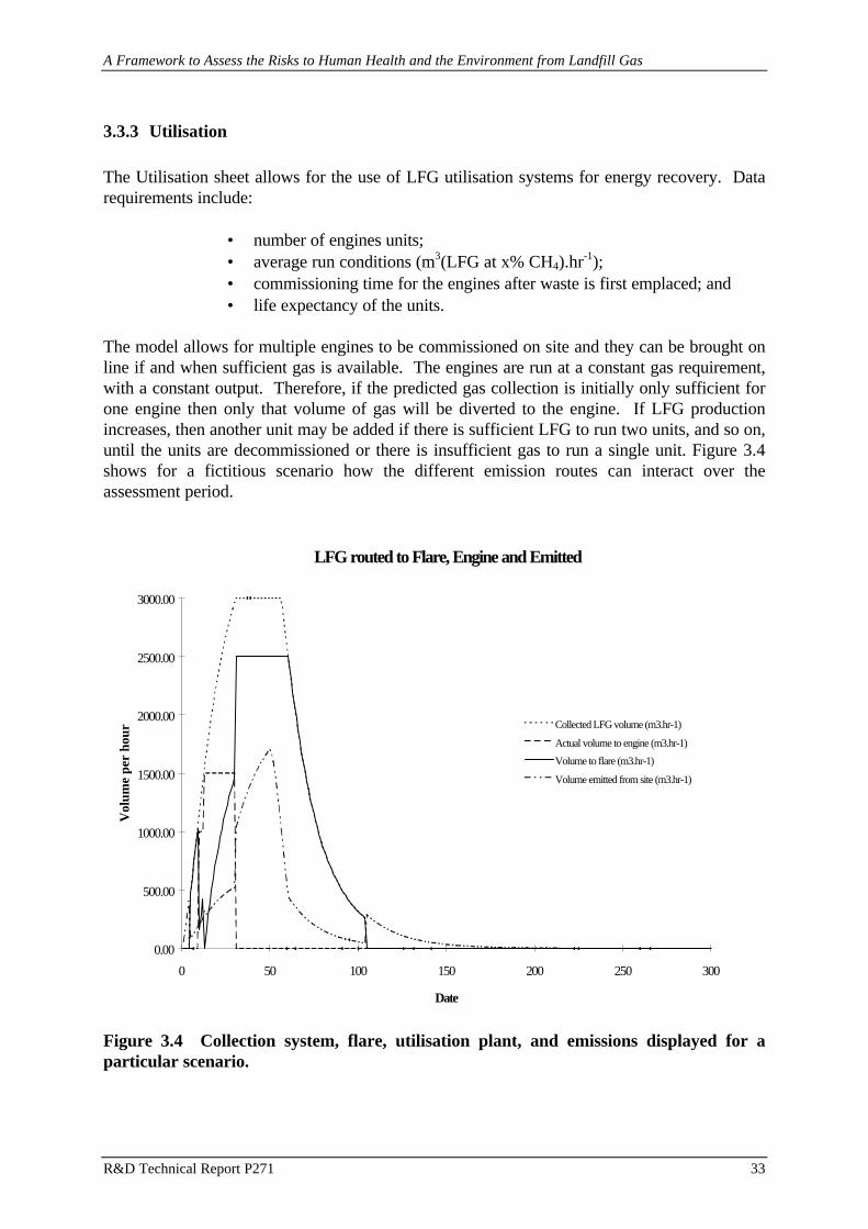
A Framework to Assess the Risks to Human Health and the Environment from Landfill Gas
R&D Technical Report P271 33
3.3.3 Utilisation
The Utilisation sheet allows for the use of LFG utilisation systems for energy recovery. Datarequirements include:
• number of engines units;• average run conditions (m3(LFG at x% CH4).hr-1);• commissioning time for the engines after waste is first emplaced; and• life expectancy of the units.
The model allows for multiple engines to be commissioned on site and they can be brought online if and when sufficient gas is available. The engines are run at a constant gas requirement,with a constant output. Therefore, if the predicted gas collection is initially only sufficient forone engine then only that volume of gas will be diverted to the engine. If LFG productionincreases, then another unit may be added if there is sufficient LFG to run two units, and so on,until the units are decommissioned or there is insufficient gas to run a single unit. Figure 3.4shows for a fictitious scenario how the different emission routes can interact over theassessment period.
LFG routed to Flare, Engine and Emitted
0.00
500.00
1000.00
1500.00
2000.00
2500.00
3000.00
0 50 100 150 200 250 300
Date
Vol
ume
per
hour
Collected LFG volume (m3.hr-1)
Actual volume to engine (m3.hr-1)
Volume to flare (m3.hr-1)
Volume emitted from site (m3.hr-1)
Figure 3.4 Collection system, flare, utilisation plant, and emissions displayed for aparticular scenario.

A Framework to Assess the Risks to Human Health and the Environment from Landfill Gas
R&D Technical Report P271 34
3.3.4 Water content of the waste
The Waste Water Content sheet allows entry of waste physical and hydrological data as well assite design details. This is used to calculate the free void space of the waste mass and thus theeffective pore volume (this is the volume available for gas to reside). The effective porevolume of the waste in conjunction with the over pressure in the site (covered below) is thenused in the calculation of Q storage for the landfill.
No migration of LFG is simulated in the saturated zone of the waste.
The water content of the waste will affect the permeability of the waste and give us an effectivepermeability. If this is greater than that of the cap or the liner then it will control the rate ofLFG migration from the site (see the section Emission Route below).
3.3.5 Emission route
Details on the site design are entered here, they include:
• cap design;• cap permeabilities;• cap thickness;• waste thickness;• waste permeabilities;• liner thickness;• liner permeability; and• site dimensions.
From these data, the layer that controls the emission rate through of the cap or liner can bedetermined, this is the layer with the lowest permeability. As mentioned previously, this maybe the waste material. The emissions from the site assume a steady state situation with all theresidual gas (that not collected) in the site being emitted. The emissions via the cap and theliner are proportional to the effective permeability of these layers and their thickness.
3.3.6 Model output
The Output sheet allows the selection of a year in the landfill life after filling has commencedand it presents data for that year. Data presented are for:
LFG production• methane production (m3.hr-1);• carbon dioxide production (m3.hr-1);• hydrogen production (m3.hr-1);• LFG production (m3.hr-1); and• cumulative production of the gases mentioned above (m3).

A Framework to Assess the Risks to Human Health and the Environment from Landfill Gas
R&D Technical Report P271 35
The Output Sheet also calculates the theoretical methane potential of the waste in m3.t-1 dryweight of waste. This is calculated over the 300 years of the assessment period, and it is auseful calculation check.
The spreadsheet also has two graphical outputs: one that shows emissions to each route inm3.hr-1; the other gives a cumulative figure in m3.
Emission routes• LFG routed to energy recovery (m3.hr-1);• LFG routed to the flare system (m3.hr-1);• LFG lost from the site in uncontrolled emissions (m3.hr-1);
∗ through the cap:∗ through the liner:
• LFG uncontrolled emission rates from the cap and liner (m3.hr-1.m-2); and• cumulative volumes of LFG to the emission routes mentioned above (m3).

A Framework to Assess the Risks to Human Health and the Environment from Landfill Gas
R&D Technical Report P271 36
4. ENVIRONMENTAL TRANSPORT
The environmental transport module deals with the following topics:
• atmospheric dispersion off-site;• atmospheric dispersion on-site;• lateral migration through the ground under steady state conditions;• lateral migration through the ground in unusual conditions (“events”).
The atmospheric dispersion parts of the module operates deterministically but takes intoaccount the probabilities of occurrence of various weather conditions. Sections 4.1 and 4.2show how this is done, describe the dispersion models used and give sources of parametervalues. In the current version of the code, lateral migration of gas through the ground understeady state conditions is modelled deterministically. The assumptions, approach andequations used are given in Section 4.3. For lateral migration under unusual conditions theapproach is to estimate the probability of occurrence of such an extraordinary migration eventbut not to attempt to estimate the consequences (see Section 4.4).
4.1 Atmospheric dispersion off-site
4.1.1 Types of models and sources
The models used to calculate pollutant concentrations in air off-site, and correspondingdeposition levels on the ground, are all of the Gaussian plume type. This type of model is usedin a variety of contexts in the UK, particularly when a number of sites are to be considered,rapid calculations are required and limited site-specific data are available. Gaussian plumemodels first began to be used more than 20 years ago and have been the subject of manyvalidation and uncertainty analysis studies.
In the dispersion calculations three types of source are considered: flares, engines and caps. Ineach case releases of pollutants to atmosphere are assumed for the purpose of dispersioncalculations to be continuous over a year. Flares and engines are treated as elevated pointsources, and for flares, plume rise resulting from thermal buoyancy is included. Caps aretreated as ground-level area sources, without any plume rise.
4.1.2 User input
User inputs to the models are:
i) the year to be considered (which the code uses to select the appropriate emissionrates of the pollutant from the results produced by the source term module);
ii) the location at which pollutant concentrations in air and deposition level on theground are to be calculated (specified as distances from the source, and directionsas points of the compass);

A Framework to Assess the Risks to Human Health and the Environment from Landfill Gas
R&D Technical Report P271 37
iii) the windrose for the site (see below);
iv) the annual frequencies of occurrence of the various Pasquill stability1 categories(see below);
v) the deposition characteristics of the pollutant (see below).
The code contains four reference windroses from which the user can choose: a uniformwindrose (the default); and three windroses based on data for sites on the west coast ofEngland, the east coast of England and central southern England. In addition there is anoption for the user to input a windrose specific to the site being considered. Four sets offrequencies of occurrence of the Pasquill stability categories are provided, one for eachwindrose, and the user has the option to input site specific data. For deposition characteristicsthe user chooses whether the pollutant being considered is to be assumed to be a non-reactivegas or a reactive gas/particulate. There is also an option for the user to input pollutant-specificvalues for the dry deposition velocity and washout coefficient. Table 4.1 shows the values ofdeposition parameters included in the code.
In the case of the location of the point of interest, the user specifies any distance (in metres) inthe range 0m to 25km. To look at on-site dispersion (see Section 4.2) the distance should beless than 10m but not zero. Directions must be specified as N, NNE, NE, NEE, E etc.
4.1.3 Equations and parameter values
The equations used for dispersion from point sources are those given in the first two reports ofa UK working group on atmospheric dispersion and which are summarised in a moreaccessible form in a recent report for the European Commission (UK Working Group onAtmospheric Dispersion 1979 and 1981; NRPB et al 1995). Equations and approximations forarea sources are taken from work for UK Nirex Ltd.
4.1.3.1 Dispersion from a point source, without deposition or plume rise
Without allowance for dry or wet deposition, or for plume rise, the mean concentration of apollutant in a sector of width α radians at a downwind distance x (m) and height z (m) from apoint source is given by:
1 A set of parameters that characterise dispersion.
Table 4.1 Values of deposition parameters
Type of material Deposition velocity, ms-1 Washout coefficient, s-1
Unreactive gases 0 0
Reactive gases, smallparticulates 10-2 10-4

A Framework to Assess the Risks to Human Health and the Environment from Landfill Gas
R&D Technical Report P271 38
In the current version of the code 30o sectors are assumed so α is π/6.
σZ , us and A vary from one stability category to another. σz and us also depend on theroughness of the ground. Values of σz are given by:
where:a, b, c, and d are constants which vary from one stability category to another (see
NRPB et al. 1995 for values),F(zo,x) is the roughness correction factor, andz0 is the roughness length.
For simplicity only one value of roughness length is used, appropriate to arable agriculturalland, allotments and gardens. This is 0.1m, in which case the roughness correction factor isunity.
NRPB et al. 1995 gives typical values of the wind speed at 10m (u10) and the mixing layerdepth for Pasquill categories A-F. The windspeed at any other height z, for a groundroughness of 0.1m, is given by:
( ) ( ) ( )X x z
Q
x u
h z A h z A h z
s
e e e
z
, exp exp exp
= −
++ −
+ ++ −
− −
0
2 2 2
2
2
2
2
2α πσ σ σ σ2 z z z2 2 2
Equation 4.1
where:
Q0 release rate from the source(mg s-1 if X is required in mg m-3)
σz standard deviation of the vertical Gaussian distribution (m)(the vertical dispersion coefficient)
us wind speed at the effective release height (m s-1)he effective release height (m)A depth of the mixing layer (m).
( )σ z
b
dax
cxF z x=
+1 0 ,
Equation 4.2
u(z) = u10 (z/10)0.2
Equation 4.3
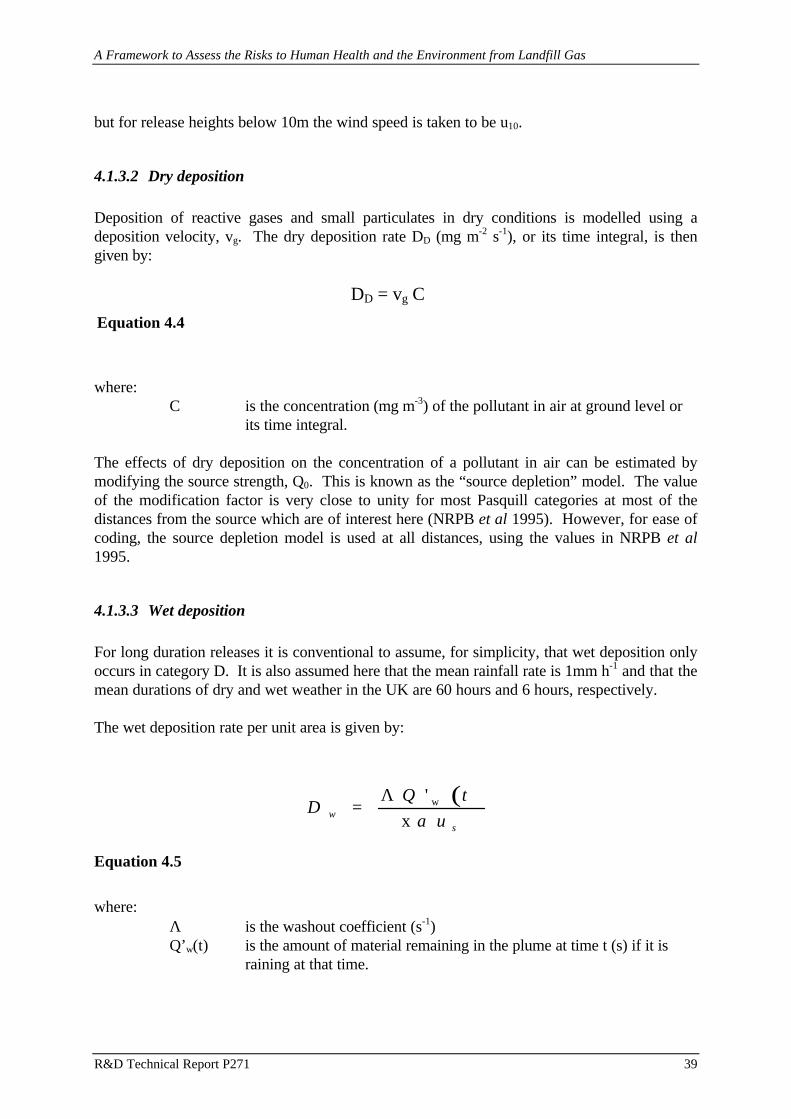
A Framework to Assess the Risks to Human Health and the Environment from Landfill Gas
R&D Technical Report P271 39
but for release heights below 10m the wind speed is taken to be u10.
4.1.3.2 Dry deposition
Deposition of reactive gases and small particulates in dry conditions is modelled using adeposition velocity, vg. The dry deposition rate DD (mg m-2 s-1), or its time integral, is thengiven by:
where:C is the concentration (mg m-3) of the pollutant in air at ground level or
its time integral.
The effects of dry deposition on the concentration of a pollutant in air can be estimated bymodifying the source strength, Q0. This is known as the “source depletion” model. The valueof the modification factor is very close to unity for most Pasquill categories at most of thedistances from the source which are of interest here (NRPB et al 1995). However, for ease ofcoding, the source depletion model is used at all distances, using the values in NRPB et al1995.
4.1.3.3 Wet deposition
For long duration releases it is conventional to assume, for simplicity, that wet deposition onlyoccurs in category D. It is also assumed here that the mean rainfall rate is 1mm h-1 and that themean durations of dry and wet weather in the UK are 60 hours and 6 hours, respectively.
The wet deposition rate per unit area is given by:
( )D
Q t
uws
=Λ '
xw
α
Equation 4.5
where:Λ is the washout coefficient (s-1)Q’w(t) is the amount of material remaining in the plume at time t (s) if it is
raining at that time.
DD = vg C
Equation 4.4

A Framework to Assess the Risks to Human Health and the Environment from Landfill Gas
R&D Technical Report P271 40
To obtain the concentration in air we need Q’(t), the amount of material remaining in theplume at time t is it has rained for part of that time. The equations for Q’w(t) and Q’(t) are:
( ) ( ) ( )[ ]Q tQ
m mm f e m f em t
wm t' =
−+ − +0
1 21 2
2 1Λ Λw
Equation 4.6
( ) ( ) ( )[ ]Q tQ
m mm e m ew
m t m t' =−
+ − +0
1 21 2
2 1Λ Λ
Equation 4.7
where:fw is the fraction of the time for which rain falls (i.e. 0.1 for the UK),
and m1 and m2 are given by:
( ) ( )
( ) ( )
2 4
2 4
1
2
2
2
m P P P P P
m P P P P P
D W D W D
D W D W D
= − + + − + + −
= − + + + + + −
Λ Λ Λ
Λ Λ Λ
where: PD is the probability of dry weather;Pw is the probability of wet weather; PD and PW are equal to the reciprocal
of the mean durations of dry and wet weather (see above).
4.1.3.4 Plume rise
To include the effects of plume rise it is sufficient to adopt a virtual release point directly abovethe actual release point, and to modify the value of σz. The effective release height in thisinstance is:
he = h + ∆h
where:∆h is derived from

A Framework to Assess the Risks to Human Health and the Environment from Landfill Gas
R&D Technical Report P271 41
∆hF
u s
b
a
=
26
13
.'
Equation 4.8
The value of σz. with plume rise is related to σzD without plume rise by
where:zp is the plume rise and is derived from:
( )z
s F s t F s t
u sp
m b
a
=+ −
3 11
21
2 1 2
2
13
' sin ' cos '
'β
Equation 4.11 (for stable conditions (categories A-C))
where: Fb is the initial buoyancy fluxua is the wind speed averaged over the height through which the plume
has risens’ is the stability parameterβ is an entrainment parameter (≈0.6)Fm is the momentum flux of the source
Further details of these parameters are given in NRPB et al 1995 (p25).
σz.2 = σzD
2 + zp2/12
Equation 4.9
zF x
u
F x
up
m
a
b
a
= +
3 3
22
2
2 3
13
β β
Equation 4.10 (for neutral and unstable conditions (categories D-F))

A Framework to Assess the Risks to Human Health and the Environment from Landfill Gas
R&D Technical Report P271 42
4.1.3.5 Averages over stability categories and wind directions D
In general the pollutant concentration in air (or the deposition rate) in direction i is given by:
Xi (r,z) = Σ fij Xij (r,z)Equation 4.12
where:fij is the frequency with which the wind blows into the sector in direction
i in stability category j, and r is the distance from the source. If only the windrose and the frequencies of stability categories are available then:
fij = fi fjwhere:
fi is the frequency with which the wind blows into sector i and fj is the frequency of occurrence of stability category j.
Then;
Xi (r,z) = fi Σ fj Xij (r,z)Equation 4.13
4.1.3.6 Dispersion from a ground level area source
For a ground level area source the average concentration of a pollutant in air (and also thedeposition rates) can be calculated by dividing the release area into strips of length L(x)perpendicular to the wind direction and integrating over the strips. In this formulation thepoint of interest is at the origin. When the wind is blowing into the same sector as the point ofinterest the concentration at ground level is:
( ) ( )X
Q
A
L x
u xdx
s zx
x0 0
20
10
, .min
max
= ∫ πασ
Equation 4.14
where:Q0 release rate from the source (mg s-1)A area of the source (m2)
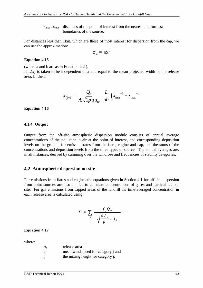
A Framework to Assess the Risks to Human Health and the Environment from Landfill Gas
R&D Technical Report P271 43
xmax , xmin distances of the point of interest from the nearest and furthest boundaries of the source.
For distances less than 1km, which are those of most interest for dispersion from the cap, wecan use the approximation:
σz = axb
Equation 4.15
(where a and b are as in Equation 4.2 ).If L(x) is taken to be independent of x and equal to the mean projected width of the releasearea, L, then:
( ) ( )XQ
A u
L
abx x
s
b b0 0
0
102, min max=
−− −
πα
Equation 4.16
4.1.4 Output
Output from the off-site atmospheric dispersion module consists of annual averageconcentrations of the pollutant in air at the point of interest, and corresponding depositionlevels on the ground, for emission rates from the flare, engine and cap, and the sums of theconcentrations and deposition levels from the three types of source. The annual averages are,in all instances, derived by summing over the windrose and frequencies of stability categories.
4.2 Atmospheric dispersion on-site
For emissions from flares and engines the equations given in Section 4.1 for off-site dispersionfrom point sources are also applied to calculate concentrations of gases and particulates on-site. For gas emissions from capped areas of the landfill the time-averaged concentration ineach release area is calculated using:
Xf Q
Au l
j
sj j
j
=
∑ 0
4
π
Equation 4.17
where:As release areauj mean wind speed for category j andlj the mixing height for category j.
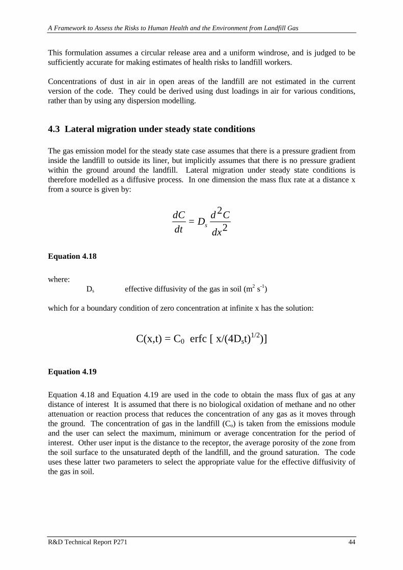
A Framework to Assess the Risks to Human Health and the Environment from Landfill Gas
R&D Technical Report P271 44
This formulation assumes a circular release area and a uniform windrose, and is judged to besufficiently accurate for making estimates of health risks to landfill workers.
Concentrations of dust in air in open areas of the landfill are not estimated in the currentversion of the code. They could be derived using dust loadings in air for various conditions,rather than by using any dispersion modelling.
4.3 Lateral migration under steady state conditions
The gas emission model for the steady state case assumes that there is a pressure gradient frominside the landfill to outside its liner, but implicitly assumes that there is no pressure gradientwithin the ground around the landfill. Lateral migration under steady state conditions istherefore modelled as a diffusive process. In one dimension the mass flux rate at a distance xfrom a source is given by:
dC
dtD
d C
dxs=
2
2
Equation 4.18
where:Ds effective diffusivity of the gas in soil (m2 s-1)
which for a boundary condition of zero concentration at infinite x has the solution:
C(x,t) = C0 erfc [ x/(4Dst)1/2)]
Equation 4.19
Equation 4.18 and Equation 4.19 are used in the code to obtain the mass flux of gas at anydistance of interest It is assumed that there is no biological oxidation of methane and no otherattenuation or reaction process that reduces the concentration of any gas as it moves throughthe ground. The concentration of gas in the landfill (Co) is taken from the emissions moduleand the user can select the maximum, minimum or average concentration for the period ofinterest. Other user input is the distance to the receptor, the average porosity of the zone fromthe soil surface to the unsaturated depth of the landfill, and the ground saturation. The codeuses these latter two parameters to select the appropriate value for the effective diffusivity ofthe gas in soil.
A Framework to Assess the Risks to Human Health and the Environment from Landfill Gas
R&D Technical Report P271 45
4.4 Lateral migration in unusual conditions
The conditions to be considered are those in which gas migration rates, and gas generationrates, increase rapidly so that there is a potential for high concentrations of flammable andtoxic gases to suddenly occur in buildings at some distance from a landfill. In such casespressure in the landfill will higher than in steady state conditions and there will be pressuredriven gas flow from the landfill through the ground. The approach used in the code is toestimate the probability that an unusual migration event will occur, given input by the userabout the presence or absence of features of the landfill and its surroundings, and about theprobabilities that various conditions exist or may do so in the future.
The features and conditions for which the user is asked to provide probabilities (aspercentages) are as follows:
• landfill is unlined• desiccation in cracks in clay liner• gas collection system out of commission for more than one day• no gas collection system• pressure drop over user defined criterion occurs• impermeable surface layer between landfill and receptor• wet or frost period occurs after a dry period, leading to an impermeable surface layer• wet or frost period occurs when gas collection sytem is out of order• strata contain fractures• fractures are linked to liner defects.
In the code these are grouped so as to obtain the probabilities that various scenarios will occur,and hence provides the user with a semi-quantitative indication of the risk of a migration eventwith severe consequences (eg an explosion in a dwelling).
A Framework to Assess the Risks to Human Health and the Environment from Landfill Gas
R&D Technical Report P271 46
5. EXPOSURE ASSESSMENT
The exposure assessment module will carry out two major functions:
• the calculation of intakes of pollutants by persons on the site or residents near thesite; and
• the calculation of concentrations of pollutants in indoor air, as a result ofatmospheric dispersion and lateral migration.
Figure 5.1 shows the information flow through these parts of the module and its interfaces withthe environmental transport and impact assessment modules. Section 5.1 describes the modelsand parameter values to be used to calculate intakes of pollutants by inhalation, ingestion anddermal exposure routes. Section 5.2 briefly indicates the models for calculating pollutantconcentrations in indoor air.
5.1 Intakes of pollutants by members of the public
In this module the exposure of residents adjacent to a landfill to chemicals in the air and viafood is assessed using assumptions about their habits and relevant data derived from theliterature. Exposure assessment of site workers could be made using the user defined‘maximally exposed individual’, with a short distance for the dispersion calculations and anoutdoor occupancy appropriate to the type of work.. However, exposure of site workersremains a health and safety at work issue rather than a public exposure issue.
In order to provide an idea of the potential range of exposures, the concepts of a “criticalgroup” and of average persons are used in the exposure assessment. A critical group has beendefined by the NRPB as “those members of the public who are most exposed from a givensource “ (NRPB 1996). This critical group, by way of its particular situation and habits, ispotentially exposed to a greater extent than the average population, and this approach thusprovides conservative estimates of exposure for assessment purposes. In addition, to providegreater flexibility, the exposure model will include a user defined “maximally exposed
For assessing the direct exposure of residents near a landfill, exposure time in and around theresidence is of greatest importance, thus the critical group is comprised of housewives andyoung children at home, and the maximally exposed individual has been chosen to be an activeretired person who spends much time gardening and little time away from home.
From this basis, the conceptual exposure model was derived for 7 types of person:
• average infant, child, and adult;• critical infant, child and adult; and• the maximally exposed individual.

A Framework to Assess the Risks to Human Health and the Environment from Landfill Gas
R&D Technical Report P271 47
All parts of the model are to be applied to each of these persons.
The exposure routes of concern to the general population living adjacent to the landfill weredefined as inhalation exposure, ingestion exposure and dermal exposure. For each of theseexposure routes, both indoor and outdoor exposures are considered and summed for eachroute.
The exposure from each route is provided as annual average exposure to the chemical and alsoas a lifetime exposure.
The chemicals to be considered in the exposure model are:
Bulk gases: methane, carbon dioxide, hydrogen.Trace gases: vinyl chloride, trichloroethene, tetrachloroethene, methane thiol,
hydrogen sulphide, dioxin, furans, chlorodifluoromethane,dichlorodifluoromethane, benzene, nitrogen oxides, sulfur oxides,hydrogen chloride, hydrogen fluoride, carbon monoxide.
Particulates: PM10, dust from landfill operation (user defined characteristics).
5.1.1 Inhalation exposure model
All the above chemicals are to be considered for the inhalation and dermal exposure routes.The bulk gases and the nitrogen oxides, sulphur oxides, hydrogen chloride, hydrogen fluorideand carbon monoxide will not be considered for the ingestion route as they are unlikely to betransported unchanged through foodchains, thus human exposure to these chemicals isimprobable via ingestion of food.
The basis for the inhalation exposure model is defined below:
EI = QI . CAIR
Equation 5.1
where:EI inhalation exposure (mg d-1)QI inhalation rate (m3 d-1)CAIR air concentration (mg m-3)
Pollutant concentrations for indoor and outdoor air will be provided from other parts of themodel (see Figure 5.1).
Following examination of the literature, inhalation rates were taken from the ICRP HumanRespiratory Tract Model (ICRP 1994), following NRPB recommendations. From theinhalation rate data in NRPB (1996), the values for 3 month and 1 year old infants have beenaveraged to provide the infant value for gas risk assessment. The 5, 10 and 15 year old datawere averaged to provide a general child value. Where separate male and female values wereprovided for 15 year olds and adults, the values have been averaged, except for the case of the

A Framework to Assess the Risks to Human Health and the Environment from Landfill Gas
R&D Technical Report P271 48
maximally exposed individual where the male adult value was chosen to provide the maximuminhalation rates for any given activity. The inhalation data for various activities
Figure 5.1 Exposure assessment module: members of the public
Impact assessment- health risk
Impact assessment- explosion risk
Depositionlevels onsoil
Calculation ofindoor air
concentrations,lateral migration
events
Calculation ofindoor air
concentrations,lateral migration at
steady state
Calculation ofindoor air
concentrations,atmosphericdispersion
Landfill migration -events
Landfill migration -steady state
Atmosphericdispersion off-site
Fluxes intobuilding- events
Fluxes intobuilding- steady state
Outdoor airconcentrations
Inhalation
DermalExposure
(skin absorptionand skin surface
effects)
Ingestion(food and soil)
Intakes byinhalation
Intakes byskinabsorption
Depositionlevels onskin
Intakes byinhalation

A Framework to Assess the Risks to Human Health and the Environment from Landfill Gas
R&D Technical Report P271 49
(sleeping, indoors, outdoors) match the categories required for gas risk assessment very well,and have been used directly apart from the averaging described above. Table 5.1 shows theinhalation rates included in the exposure assessment module.
Table 5.1 Inhalation rates (m3hr-1)
PopulationActivity Average group Critical group Maximally
Infant0-1 yr
Child1-16 yr
Adult16-70 yr
Infant0-1 yr
Child1-16 yr
Adult16-70 yr
exposedindividual
Indoors at home sleep 0.12 0.31 0.39 0.12 0.31 0.39 0.45other 0.25 0.75 1.07 0.25 0.75 1.07 1.18
Outdoors at home 0.31 0.94 1.11 0.31 0.94 1.11 1.69
(Away from home) 0.25 0.75 1.07 0.25 0.75 1.07 1.18
The above matrix of inhalation rates for various populations and activities (NRPB 1996) mustbe combined with estimates of occupancy times for each location and activity to provideinhalation data in units of m3 per day. Occupancy data describing the time spent indoors oroutdoors at home and away from home has been taken from NRPB (1987) utilising dataderived from a BBC survey on population activity conducted in 1978 (BBC 1978). Morerecent data on domestic occupancy has not been found. The data in this report was used toascertain that housewives would form the critical group for a pollution source adjacent to adomestic residence; young pre-school children would also have the same high domesticoccupancy as the housewives. The critical group occupancy data has thus been derived fromthe housewife data in the report. The average population data has been derived from thereport with some estimations made regarding the time spent outside at home for this group.The report also provides the data on sleeping time, school hours and time away from home forthe relevant populations. The maximally exposed individual has been based on housewifeoccupancy data but with more time spent outdoors at home (e.g. gardening) rather thanindoors or away from home, as this provides higher inhalation rates and probably greaterexposure to higher outdoor air concentrations, though this may be chemical dependent.Table 5.2 shows the derived occupancy data to be used in the module.
Table 5.2 Occupancy rates (hr day-1)
PopulationActivity Average group Critical group Maximally
Infant0-1 yr
Child1-16 yr
Adult16-70 yr
Infant0-1 yr
Child1-16 yr
Adult16-70 yr
exposedindividual
Indoors at home sleep 14 10 8 14 10 8 8other 7 9.5 11 7 9 12.5 12
Outdoors at home 0.5 0.5 0.5 1 1 1 3
(Away from home) 2.5 4 4.5 2 4 2.5 1

A Framework to Assess the Risks to Human Health and the Environment from Landfill Gas
R&D Technical Report P271 50
The data in these two tables can be combined for each population set to provide a table ofactivity weighted inhalation rates (m3 d-1) as follows:
QIA = A . QI/hr
Equation 5.2
where:QIA activity weighted inhalation rate (m3 d-1)A activity (hr d-1)QI/hr inhalation rate (m3 hr-1)
This provides values for average, activity weighted inhalation rates as shown in Table 5.3.
Table 5.3 Activity weighted inhalation at home (m3 day-1)
PopulationActivity Average group Critical group Maximally
Infant0-1 yr
Child1-16 yr
Adult16-70 yr
Infant0-1 yr
Child1-16 yr
Adult16-70 yr
exposedindividual
Indoors at home sleep 1.68 3.10 3.12 1.68 3.10 3.12 3.60other 1.75 7.13 11.77 1.75 6.75 13.38 14.16
Outdoors at home 0.16 0.47 0.56 0.31 0.94 1.11 5.07
(Away from home) (0.63) (3.00) (4.82) (0.50) (3.00) (2.68) (1.18)
Total at home inhalation(m3 d-1)
3.59 10.70 15.45 3.74 10.79 17.61 22.83
The at home inhalation data can be multiplied by 365 to provide m3 yr-1, which can then becombined with the indoor and outdoor annual average air concentrations for each chemical.Annual average (mg yr-1) and cumulative lifetime (mg lifetime-1) exposures via inhalation canthen be derived for any of the population groups over any given time period of the landfilllifetime. A lifetime has been set at 70 years.
5.1.2 Ingestion exposure model
The ingestion exposure model includes ingestion of locally produced or home-grownfoodstuffs and, additionally, inadvertent ingestion of soil and house dust. Ingestion exposurevia foodstuffs can be described by
EIN = QIN local . C food
Equation 5.3
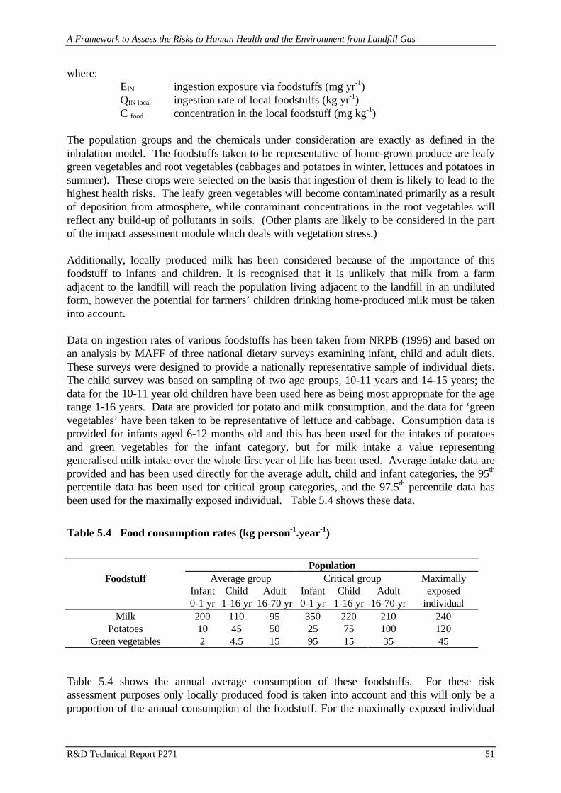
A Framework to Assess the Risks to Human Health and the Environment from Landfill Gas
R&D Technical Report P271 51
where:EIN ingestion exposure via foodstuffs (mg yr-1)QIN local ingestion rate of local foodstuffs (kg yr-1) C food concentration in the local foodstuff (mg kg-1)
The population groups and the chemicals under consideration are exactly as defined in theinhalation model. The foodstuffs taken to be representative of home-grown produce are leafygreen vegetables and root vegetables (cabbages and potatoes in winter, lettuces and potatoes insummer). These crops were selected on the basis that ingestion of them is likely to lead to thehighest health risks. The leafy green vegetables will become contaminated primarily as a resultof deposition from atmosphere, while contaminant concentrations in the root vegetables willreflect any build-up of pollutants in soils. (Other plants are likely to be considered in the partof the impact assessment module which deals with vegetation stress.)
Additionally, locally produced milk has been considered because of the importance of thisfoodstuff to infants and children. It is recognised that it is unlikely that milk from a farmadjacent to the landfill will reach the population living adjacent to the landfill in an undilutedform, however the potential for farmers’ children drinking home-produced milk must be takeninto account.
Data on ingestion rates of various foodstuffs has been taken from NRPB (1996) and based onan analysis by MAFF of three national dietary surveys examining infant, child and adult diets.These surveys were designed to provide a nationally representative sample of individual diets.The child survey was based on sampling of two age groups, 10-11 years and 14-15 years; thedata for the 10-11 year old children have been used here as being most appropriate for the agerange 1-16 years. Data are provided for potato and milk consumption, and the data for ‘greenvegetables’ have been taken to be representative of lettuce and cabbage. Consumption data isprovided for infants aged 6-12 months old and this has been used for the intakes of potatoesand green vegetables for the infant category, but for milk intake a value representinggeneralised milk intake over the whole first year of life has been used. Average intake data areprovided and has been used directly for the average adult, child and infant categories, the 95th
percentile data has been used for critical group categories, and the 97.5th percentile data hasbeen used for the maximally exposed individual. Table 5.4 shows these data.
Table 5.4 shows the annual average consumption of these foodstuffs. For these riskassessment purposes only locally produced food is taken into account and this will only be aproportion of the annual consumption of the foodstuff. For the maximally exposed individual
Table 5.4 Food consumption rates (kg person-1.year-1)
PopulationFoodstuff Average group Critical group Maximally
Infant0-1 yr
Child1-16 yr
Adult16-70 yr
Infant0-1 yr
Child1-16 yr
Adult16-70 yr
exposedindividual
Milk 200 110 95 350 220 210 240Potatoes 10 45 50 25 75 100 120
Green vegetables 2 4.5 15 95 15 35 45
A Framework to Assess the Risks to Human Health and the Environment from Landfill Gas
R&D Technical Report P271 52
and the critical group, it may be prudent to assume that their total consumption of thesefoodstuffs is home-grown or local. For the average population it is suggested that 50% oftotal consumption is of home-grown or local produce (MAFF, personal communication,Walters, 1995). Thus local food consumption rates can be derived by multiplying the totalfood consumption rates by the proportion of this which is home-grown.
QIN local = QIN . h
Equation 5.4
where:QIN local ingestion rate of local foodstuffs (kg yr-1) QIN total food ingestion rate (kg yr-1)h proportion of home-grown produce (unitless)
These food consumption rates are then combined with the concentration of the chemical inparticular foodstuffs to provide an ingestion exposure from home-grown vegetables and locallyproduced milk.
EIN = QIN local . C food
Equation 5.5
where:EIN ingestion exposure via foodstuffs (mg yr-1)QIN local ingestion rate of local foodstuffs (kg yr-1) C food concentration in the local foodstuff (mg kg-1)
In order to obtain data on the chemical contamination of the locally produced foodstuffs it isnecessary to simulate the movement of the chemicals through to foodstuff following depositionfrom atmosphere. It is assumed that chemicals from the landfill will be deposited on both thesoil and vegetation, and thus be present in garden produce via root uptake, stomatal uptakeand direct contamination of the leaves. To obtain an estimate of the transfer of chemicalsthrough the foodchain the concept of transfer factors are used where equilibriumconcentrations of a chemical in soil is linked to concentrations in the vegetation growing onthat soil by a linear factor. The factor is thus a method of taking all the potential transferroutes to vegetation into account in one equation.
Bv = C dry plant / C dry soil
Equation 5.6
where:Bv transfer factor soil to plantC dry plant concentration in dry plant (mg kg-1)C dry soil concentration in dry soil (mg kg-1)
and

A Framework to Assess the Risks to Human Health and the Environment from Landfill Gas
R&D Technical Report P271 53
Bm = C dry milk / DI
Equation 5.7
where:Bm transfer factor plant to milkC dry milk concentration in dry milk (mg kg-1)DI daily intake of chemical (mg d-1)
For various organic chemicals, a relationship between the octanol-water partition coefficient(Kow) of the chemical and its measured transfer factor (Bv) to vegetation and to milk (Bm) hasbeen derived by Travis and Arms (1988). These derived values have been used here to obtaintransfer factors for the trace volatile organic chemicals which are released from landfills.Where it has been possible to obtain a value for the octanol-water partition coefficient of achemical, this has been used to model the transfer of these chemicals through the soil tovegetation and then to milk using the following relationships derived from Travis and Arms(1988).
log Bv = 1.588 - 0.578 log Kow
Equation 5.8
and
log Bm = -8.10 + log Kow
Equation 5.9
Octanol-water partition coefficients have been determined for most of the volatile organicchemicals and these are shown in Table 5.5. When soil concentrations of the chemicals areavailable from the deposition model, the derived transfer factors, Bv and Bm, described abovecan be used to provide the chemical concentrations in the vegetation and then milk. Thesecalculations have been included in the module. Soil concentrations will be provided from thedeposition module for each chemical to be considered. Deposition of chemicals to soil (mg m-
2) will be averaged through the top 20 cm depth of soil (the rooting zone) to provide aconcentration in the rooting zone (mg m-3 to 20 cm depth).
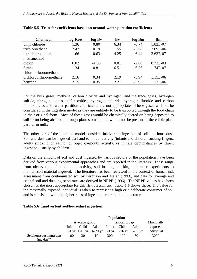
A Framework to Assess the Risks to Human Health and the Environment from Landfill Gas
R&D Technical Report P271 54
For the bulk gases, methane, carbon dioxide and hydrogen, and the trace gases, hydrogensulfide, nitrogen oxides, sulfur oxides, hydrogen chloride, hydrogen fluoride and carbonmonoxide, octanol-water partition coefficients are not appropriate. These gases will not beconsidered in the ingestion model as they are unlikely to be transported through the food chainin their original form. Most of these gases would be chemically altered on being deposited tosoil or on being absorbed through plant stomata, and would not be present in the edible plantpart, or in milk.
The other part of the ingestion model considers inadvertent ingestion of soil and housedust.Soil and dust can be ingested via hand-to-mouth activity (infants and children sucking fingers,adults smoking or eating) or object-to-mouth activity, or in rare circumstances by directingestion, usually by children.
Data on the amount of soil and dust ingested by various sectors of the population have beenderived from various experimental approaches and are reported in the literature. These rangefrom observation of hand-mouth activity, soil loading on skin, and tracer experiments tomonitor soil material ingested. The literature has been reviewed in the context of human riskassessment from contaminated soil by Ferguson and Marsh (1993), and data for average andcritical soil and dust ingestion rates are derived in NRPB (1996). The NRPB values have beenchosen as the most appropriate for this risk assessment. Table 5.6 shows these. The value forthe maximally exposed individual is taken to represent a high or a deliberate consumer of soiland is consistent with the higher rates of ingestion recorded in the literature.
Table 5.6 Inadvertent soil/housedust ingestion
PopulationAverage group Critical group Maximally
Infant0-1 yr
Child1-16 yr
Adult16-70 yr
Infant0-1 yr
Child1-16 yr
Adult16-70 yr
exposedindividual
Soil/housedust ingestion(mg day-1)
100 30 10 300 100 30 3000
Table 5.5 Transfer coefficients based on octanol-water partition coefficients
Chemical log Kow log Bv Bv log Bm Bmvinyl chloride 1.36 0.80 6.34 -6.74 1.82E-07trichloroethene 2.42 0.19 1.55 -5.68 2.09E-06tetrachloroethene 1.66 0.63 4.25 -6.44 3.63E-07methanethioldioxin 6.02 -1.89 0.01 -2.08 8.32E-03furans 1.34 0.81 6.51 -6.76 1.74E-07chlorodifluoromethanedichlorodifluoromethane 2.16 0.34 2.19 -5.94 1.15E-06benzene 2.15 0.35 2.21 -5.95 1.12E-06
A Framework to Assess the Risks to Human Health and the Environment from Landfill Gas
R&D Technical Report P271 55
These values of soil ingestion will be combined with the concentration of chemicals in the dustto provide information on the amount of chemical ingested per day and then per year.
5.1.3 Dermal exposure model
For the gases released from landfill, dermal exposure will be related to the concentration of thegas in air and to the deposition velocity of the gas concerned which is to be provided fromother parts of the model, and also to the surface area of the skin available for deposition. Forgases the assumption has been made that no attenuation of deposition would occur due toclothing. This may be conservative, but gases have the ability to permeate most materials.There would also have to be a time weighting for indoor and outdoor exposure depending onthe occupancy rates provided in the inhalation model and the indoor and outdoor airconcentration.
The adult skin area for an adult is provided as 18,150 cm2 (average of male and female ages20-30 years, USEPA 1988a), and for a child is provided as 9,400 cm2 (average of male andfemale ages 3-12 years, USEPA 1988b).
For particulate releases from landfill, direct dermal exposure to PM10 may pose a health risk inthe same way as gaseous dermal exposure and this can be assessed by the deposition velocityroute outlined above. Additionally particulates may act as carriers for other chemicals such asheavy metals and other organic chemicals and this can be assessed using dust adherence data,chemical loading of the dust and exposed skin areas.
5.2 Calculation of pollutant concentrations in indoor air
As indicated in Figure 5.1, models are needed to calculate pollutant concentrations in indoorair resulting from atmospheric dispersion of emissions from the landfill cap, flares andutilisation plant, and from lateral migration of gases through the ground. In the migration casewe need to consider steady state conditions and unusual conditions.
The current module enables the user to consider several types of design of houses, spanningthe range from modern houses with slab floors to old houses with cellars. Two main types ofhouse construction have been modelled, one is a slab based building, the other is a buildingwith a suspended floor. The first type allows consideration of modern concrete flooredbuildings, but would also cover brick floors on soil in older houses and other forms ofconstruction where there is no void space between the soil and the living space (Figure 5.2).The second type of model considers a space beneath a suspended floor and the airconcentrations are calculated in the lower space as well as in the living space above (Figure5.3). This methodology covers houses with cellars or access space beneath the building andthose with suspended floors. Many older houses would fall into this category. Changing theinput parameters regarding dimensions of the building allows the user to model different formsof building constructions with these two approaches.

A Framework to Assess the Risks to Human Health and the Environment from Landfill Gas
R&D Technical Report P271 56
Equations have been derived to calculate indoor concentrations from soil gas concentrations(available from the lateral migration model) and outdoor air concentrations (available from theatmospheric dispersion models). Data has been acquired for the calculations although it isrecognised that derivation of parameter values for typical UK houses is likely to be a matter ofjudgement. Default parameter values are provided in the HELGA User Manual.
Slab based buildings
C2 = (D12 + α)C1 + βC3
D12 + β
Equation 5.10
where:
α = VsPL/(SaA)
β = D23(w) (Awa - Awd)/A + D23( c) + Exh
C1 concentration of contaminant in soil gasC2 concentration of contaminant in indoor airC3 concentration of contaminant in outdoor airD12 coefficient of molecular diffusion between the soil and the living spaceD23(w) coefficient of molecular diffusion between the living space and outdoor air
through building wallsD23( c) coefficient of molecular diffusion between the living space and outdoor air
through building ceilingVs suction flow velocityP perimeter length of houseL character length over which suction flow is effectiveSa air filled soil porosityA ground area of houseAwa area of house wallsAwd area of external windows and doorsEx air exchange rate in living spaceh height of living space
The equation for the suspended floor building is an extension of the slab based floor modeldescribed above. It includes a sub-floor space and calculates the diffusion between this volumeand the house ground floor (Figure 5.3). Many of the input parameters are the same as thoselisted for the slab based floor equations, with additional information required for thedimensions of the sub-floor void.
For the case of lateral migration under unusual conditions the concern is to determine whethergas concentrations could build up to levels where the risk of explosion is high, or where thereis a possibility of sudden, serious health effects (e.g. asphyxiation). The equations used for

A Framework to Assess the Risks to Human Health and the Environment from Landfill Gas
R&D Technical Report P271 57
steady state conditions can be adapted for use to calculate air concentrations in the unusualconditions of weather and lateral migration which are relevant.
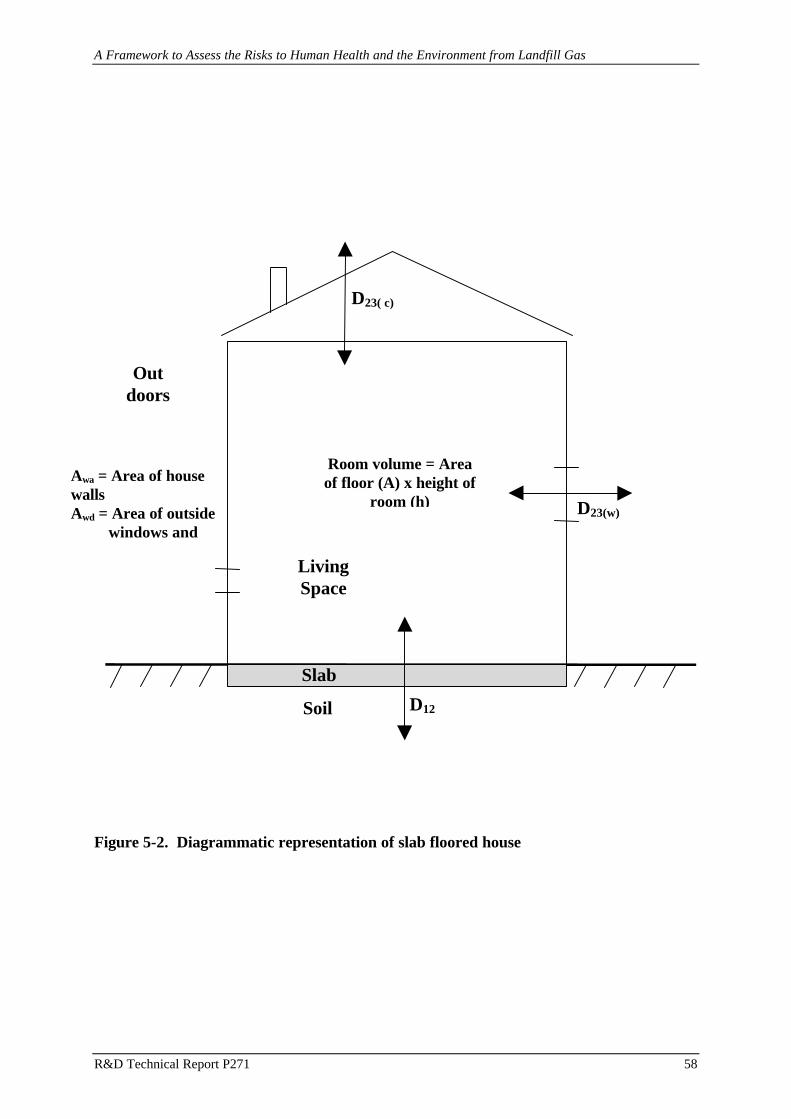
A Framework to Assess the Risks to Human Health and the Environment from Landfill Gas
R&D Technical Report P271 58
Awa = Area of housewallsAwd = Area of outside
windows and
D12
D23(w)
D23( c)
Room volume = Areaof floor (A) x height of
room (h)
Soil
Slab
LivingSpace
Outdoors
Figure 5-2. Diagrammatic representation of slab floored house

A Framework to Assess the Risks to Human Health and the Environment from Landfill Gas
R&D Technical Report P271 59
Figure 5-3. Diagrammatic representation of a suspended floor building
Awa2 = Area of housewallsAwd = Area of outside
windows and
D01
D23(w)
D23( c)
Living Space volume =Area of floor (A) x height
(H2)
Soil
LivingSpace
Outdoors
D12
D13CrawlingSpace
Crawling Space volume =Area of floor (A) x height
(H1)Awa1 = Area of walls in
crawling space

A Framework to Assess the Risks to Human Health and the Environment from Landfill Gas
R&D Technical Report P271 60
6. VALIDATION TESTS FOR THE HELGA MODULES
6.1 Introduction
In order to provide confirmation that the calibrated HELGA modules bear resemblance toactual behaviour, and can therefore be used with confidence to forecast behaviour at otherlandfill sites, a series of validation trials were carried out. The concept behind validationtesting is that model forecast data are compared with data which have been derived by othermeans than modelling. The degree of consistency between the two data sets demonstrates thevalidity of the model forecasting capability.
It is not necessary to validate all aspects of the model on one site. Indeed, there is no singlesite which could provide sufficient data to test all emission pathways represented in theHELGA model. The approach adopted was to investigate each key module or pathway withreference to a well characterised set of site measurements. The validation tests concentrate onthe modules which need to be tested, i.e. those which generate the concentration of the emittedpollutant under consideration at a given distance from the landfill. These modules aregenerally those which are concerned with generation, emission and migration. The impactassessment modules are all based on given exposure levels, and so cannot be validated in thisfashion.
The following tests were performed (see Table 6.1).
Table 6.1. Validation tests for HELGA modules
Landfill Site Module(s)evaluated
Description
Auchencarrochtest cells
Gas generation Well-monitored test cells were used to provide datafor the gas generation (source-term) module ofHELGA.
UnidentifiedBuckinghamshirelandfill
Gas generation andSurface emissions -methane
Data from part of a well characterised site inBuckinghamshire were compared with equivalentdata from other sites in the UK, to test theemissions module for methane.
Greene Valleylandfill (US)
Surface emissions -VOCs
A suite of comprehensive monitoring data from thisUS landfill was compared with forecast emissions,to test the emissions module for VOCs.
Nant-y-Gwyddonlandfill
Atmosphericdispersion
This site has been well characterised in terms ofodour characteristics. Hydrogen sulphidedispersion modelling was compared with sitemonitoring data.
Foxhall landfill Lateral migration This well characterised site has demonstrated somelateral off-site gas and VOC migration. The modelforecasts were compared to measuredconcentrations off site, along the line of the plume.
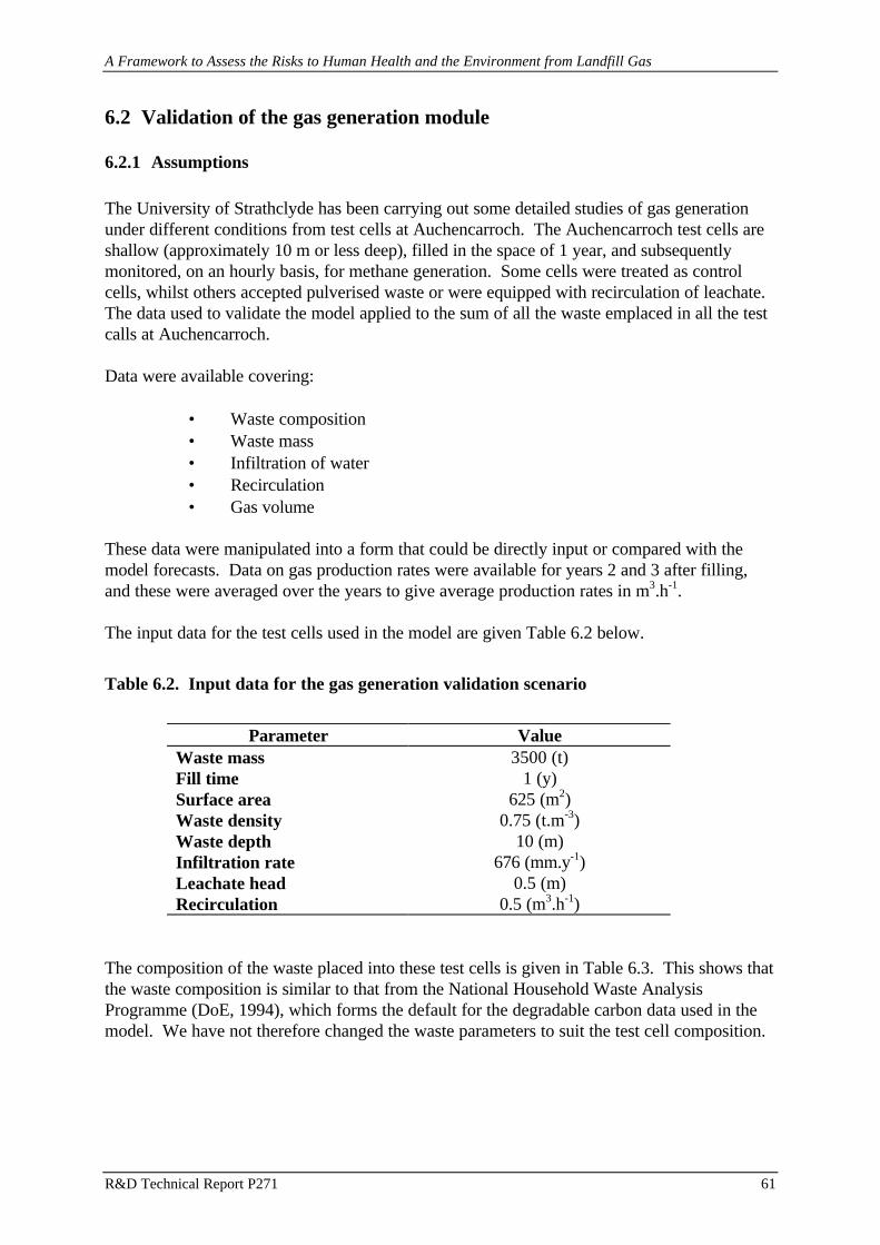
A Framework to Assess the Risks to Human Health and the Environment from Landfill Gas
R&D Technical Report P271 61
6.2 Validation of the gas generation module
6.2.1 Assumptions
The University of Strathclyde has been carrying out some detailed studies of gas generationunder different conditions from test cells at Auchencarroch. The Auchencarroch test cells areshallow (approximately 10 m or less deep), filled in the space of 1 year, and subsequentlymonitored, on an hourly basis, for methane generation. Some cells were treated as controlcells, whilst others accepted pulverised waste or were equipped with recirculation of leachate.The data used to validate the model applied to the sum of all the waste emplaced in all the testcalls at Auchencarroch.
Data were available covering:
• Waste composition• Waste mass• Infiltration of water• Recirculation• Gas volume
These data were manipulated into a form that could be directly input or compared with themodel forecasts. Data on gas production rates were available for years 2 and 3 after filling,and these were averaged over the years to give average production rates in m3.h-1.
The input data for the test cells used in the model are given Table 6.2 below.
Table 6.2. Input data for the gas generation validation scenario
Parameter ValueWaste mass 3500 (t)Fill time 1 (y)Surface area 625 (m2)Waste density 0.75 (t.m-3)Waste depth 10 (m)Infiltration rate 676 (mm.y-1)Leachate head 0.5 (m)Recirculation 0.5 (m3.h-1)
The composition of the waste placed into these test cells is given in Table 6.3. This shows thatthe waste composition is similar to that from the National Household Waste AnalysisProgramme (DoE, 1994), which forms the default for the degradable carbon data used in themodel. We have not therefore changed the waste parameters to suit the test cell composition.

A Framework to Assess the Risks to Human Health and the Environment from Landfill Gas
R&D Technical Report P271 62
Table 6.3. Waste composition placed in the test cells and from the National HouseholdWaste Analysis Programme (NHWAP. DoE, 1994).
Waste Category Untreated Pulverised NHWAPPaper/Card 27.29 32.65 33.49Plastic Film 5.64 7.25 5.09Dense Plastic 5.20 8.35 5.34Textiles 3.67 3.65 2.36Misc. Combustibles 3.54 3.45 7.94Misc. Non-combustibles 0.50 1.75 2.02Glass 4.67 6.40 8.63Putrescibles 38.40 24.65 20.79Ferrous Metals 5.88 8.05 6.32Non-ferrous Metals 0.87 1.55 1.44Fines 4.39 2.20 7.11
6.2.2 Validation Results
The range of modelled LFG production rates for years 2 and 3 are shown in Table 6.4. Thesedata can be compared with the experimental results for the LFG production in the test cells,which are given in Table 6.5.
Table 6.4. Modelled LFG production rates from the test cells (m3 h-1)
Year Max Mean Min Range1 19.5 15 10.5 9.02 9.7 8 6.3 3.43 5.4 4.8 4.1 1.3
Table 6.5. Experimentally determined LFG production rates from the test cells (m3 h-1)
Year Cell 1 Cell 2 Cell 3 Cell 42 8.47 5.80 5.68 5.483 5.27 3.67 3.52 5.51
Figure shows the model output, with the experimental data overlain. The figure shows themean LFG production rate from the test cells (black dot), the range of results (rectangular box)and one standard deviation either side of the mean (black bar line). The HELGA forecast dataare shown as three curves (mean - square symbols; 5th percentile - triangles; 95th percentile -diamonds).
Degradation rates have been chosen which are quite rapid, to reflect recirculation of leachateand pulverisation of the waste prior to landfilling. The results show that the model andexperimental ranges overlap for years 2 and 3. This therefore indicates that the model

A Framework to Assess the Risks to Human Health and the Environment from Landfill Gas
R&D Technical Report P271 63
produces results that are within the range of the experimental data. This is encouraging, as gasgeneration in the early years has been notoriously difficult both to forecast, and measure.
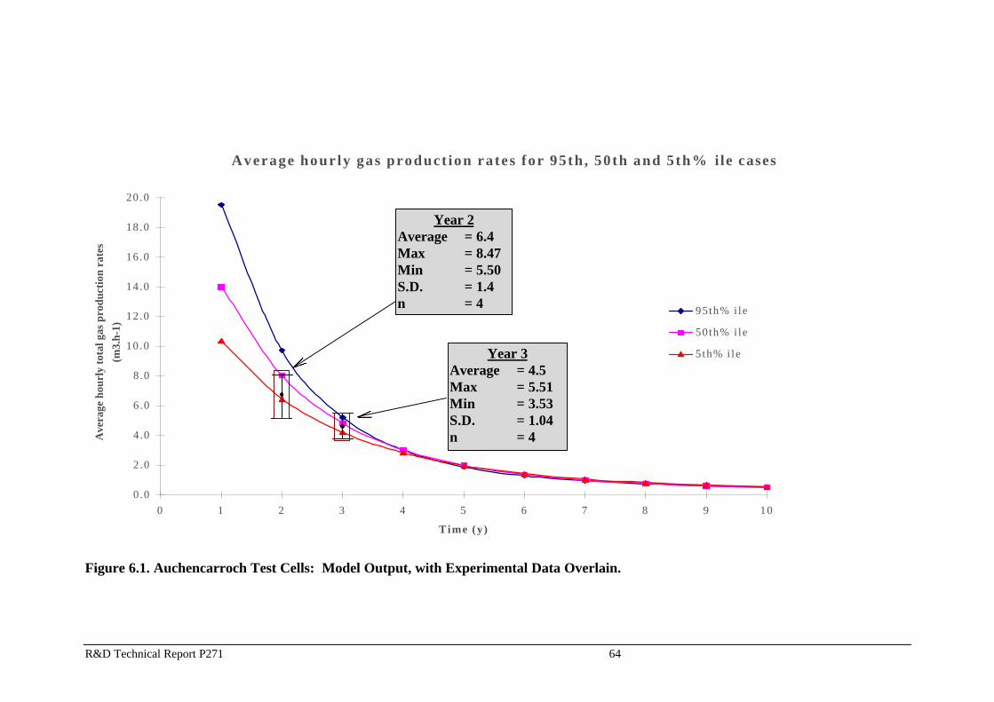
R&D Technical Report P271 64
Average hourly gas product ion rates for 95th , 50th and 5th% ile cases
0.0
2.0
4.0
6.0
8.0
10.0
12.0
14.0
16.0
18.0
20.0
0 1 2 3 4 5 6 7 8 9 10
Time (y )
Ave
rage
hou
rly
tota
l gas
pro
duct
ion
rate
s
(m3.
h-1)
95th% i le
50th% i le
5 th% i le
Figure 6.1. Auchencarroch Test Cells: Model Output, with Experimental Data Overlain.
Year 2Average = 6.4Max = 8.47Min = 5.50S.D. = 1.4n = 4
Year 3Average = 4.5Max = 5.51Min = 3.53S.D. = 1.04n = 4

A Framework to Assess the Risks to Human Health and the Environment from Landfill Gas
R&D Technical Report P271 65
6.3 Validation of gas generation module and surface emission of methane
6.3.1 Assumptions
This Buckinghamshire landfill (otherwise unidentified) has accepted predominantly domesticwaste for many years. For the phase of landfilling under consideration, waste was emplacedbetween 1978 and 1985. Table 6.6 gives the model input data for this scenario.
Table 6.6. Input data for the methane surface emissions scenario
Parameter ValueVolume of waste into site 2,000,000 (t)Waste composition 100% domesticFilling of site 1978 to 1985Waste type for model (Era) 2 (current)Fill regime (average for years):78/79 200,000 (t.y-1)80/81 200,000 (t.y-1)82/83 260,000 (t.y-1)84/85 333,000 (t.y-1)Saturation of waste wetSurface capping 1m clay and 0.8m soil for agricultural
purposesLandfill gas (LFG) collection fromarea modelled (in 1997)
700 to 1000 (m3.h-1)
6.3.2 Validation results
Landfill gas production
Two model interpolations have been carried out. The first simulation uses the pseudo-probabilistic version of the HELGA model, as delivered to the Environment Agency, which isnot dependent upon Crystal BallTM add-in software. The second uses the fully probabilisticmode, which is expected to be used in subsequent versions of the model. The pseudoprobabilistic mode built into the framework model allows HELGA to be used without theseparate Crystal BallTM probability sampling package.
Figure 6.2 shows the pseudo probabilistic model output for the first 30 years. The forecastrange of LFG production rates for the time period 18 to 20 years after filling commenced isshown by the box labelled ‘forecast data’. The actual site LFG production (assuming gascollection = gas production) is shown by the box labelled ‘observed data’. Figure 6.2therefore shows that, in this case, the HELGA model is underestimating the LFG productionrate by about 28%.

A Framework to Assess the Risks to Human Health and the Environment from Landfill Gas
R&D Technical Report P271 66
Average hourly gas production rates for 95th%, 50th% and 5th% cases
0.0
500.0
1000.0
1500.0
2000.0
2500.0
3000.0
3500.0
0 2 4 6 8 10 12 14 16 18 20 22 24 26 28 30
Time (y)
Ave
rage
hou
rly
tota
l gas
pro
duct
ion
rate
s (m
3.h-
1)
Total (95th%)
Total (50th%)
Total (5th%)
model forecast
observed range
Number of years after which assessment of gas production is made
Figure 6.2. Pseudo-probabilistic output, comparing landfill gas production after 18 to20 years (observed range) and the modelled landfill gas production rate (modelforecast)).
If, however, the fully probabilistic Crystal Ball ™ mode is used (Figure 6.3), the estimatedrange of LFG production from the site and the modelled range overlap. This limited validationindicates that both the pseudo-probabilistic model and the fully probabilistic model produceresults that are reasonably close to field data.
Crystal Ball Simulation results for LFG production (each point average of 5 years)
0
200
400
600
800
1000
1200
1400
1600
1800
2000
0 2 4 6 8 10 12 14 16 18 20 22 24 26 28 30
Year
LF
G (
m3/
hr)
5.0%
50.0%
95.0%
observed range
model forecast
Figure 6.3. Fully probabilistic output, with landfill gas production after 18 to 20 years(observed range) and modelled landfill gas production rates (model forecast).

A Framework to Assess the Risks to Human Health and the Environment from Landfill Gas
R&D Technical Report P271 67
As would be expected, the fully probabilistic model appears to deal better with uncertainties ininput data and assumptions to produce a range that matches better the field data.
Surface methane emissions
Surface methane emissions from the Buckinghamshire site have also been determined in themodel for the selected time frame (18 to 20 years after filling commenced). The two scenariosconsidered below are:
• Scenario 1: 85% LFG collection efficiency and 70% biological oxidation of fugitivemethane in the cap.
• Scenario 2: 95% LFG collection efficiency and 90% biological oxidation of fugitivemethane in the cap.
The HELGA model calculates average net surface methane emissions after allowing for LFGcollection and biological methane oxidation. The model output indicates the average surfaceemissions from this site would be between 10-2 mg.m2.s-1 (Scenario 1) and 10-3 mg.m2.s-1
(Scenario 2) (Figure 6.4). Although site measurements were not available for this landfill, fieldmeasurements of methane flux from a number of other, similar, sites indicate that for a landfillwith an engineered cap and gas collection scheme the average net emissions are in the range of10-4 to 1 mg.m2.s-1 (Gregory et al., 1998; Milton et al., 1997) This range of measuredemissions is consistent with other published studies (Bogner et al., 1997a).
Figure 6.4 compares the range of measured data with modelled data. The ranges overlap. Thissuggests that (1) the HELGA model is calculating results within the expected ranges, and(2) more work is required to characterise and understand the different results produced bydifferent methane flux protocols.
Figure 6.4. Surface emissions data modelled for site scenarios 1 and 2 (black crosses)superimposed on field results for similar sites (WS Atkins flux box measurements, andNPL above-surface emissions measurements).
10-4 10-3 10-210-1 100
Methane flux mg/m2/s-1
Flux-boxmeasurements
Model forecast for Scenario 2
Above-surface emissionsmeasurements
Model forecast for Scenario 1
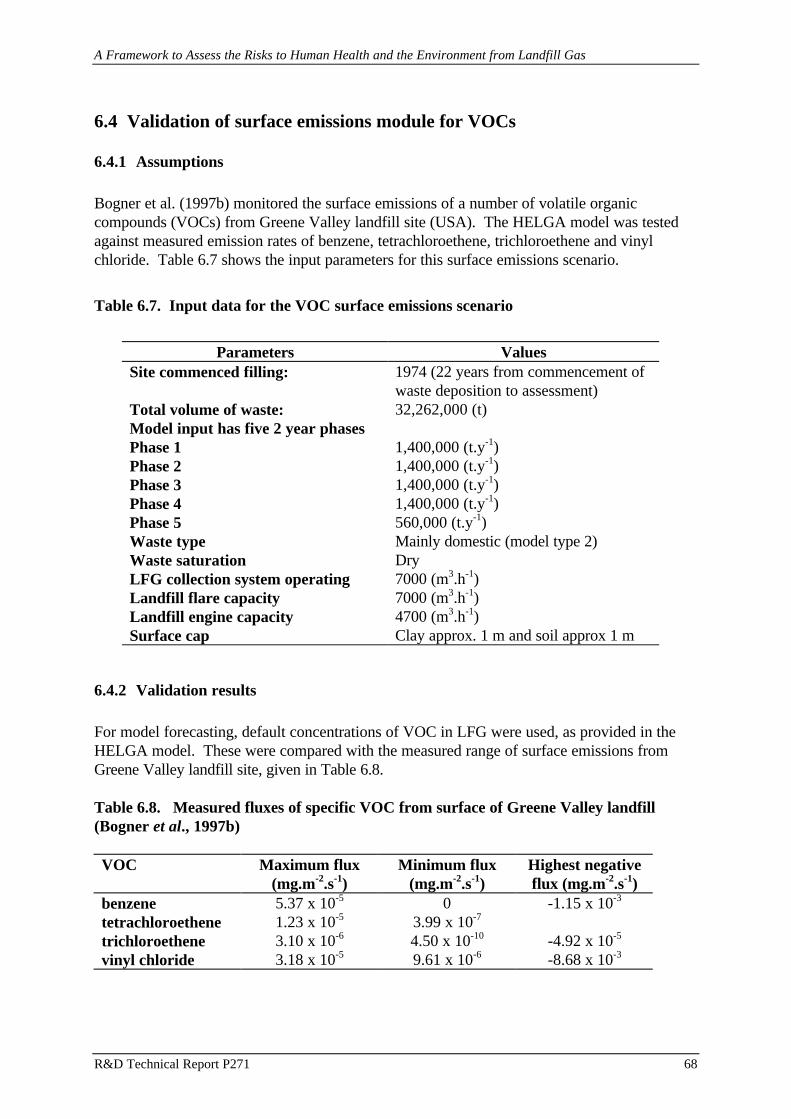
A Framework to Assess the Risks to Human Health and the Environment from Landfill Gas
R&D Technical Report P271 68
6.4 Validation of surface emissions module for VOCs
6.4.1 Assumptions
Bogner et al. (1997b) monitored the surface emissions of a number of volatile organiccompounds (VOCs) from Greene Valley landfill site (USA). The HELGA model was testedagainst measured emission rates of benzene, tetrachloroethene, trichloroethene and vinylchloride. Table 6.7 shows the input parameters for this surface emissions scenario.
Table 6.7. Input data for the VOC surface emissions scenario
Parameters ValuesSite commenced filling: 1974 (22 years from commencement of
waste deposition to assessment)Total volume of waste: 32,262,000 (t)Model input has five 2 year phasesPhase 1 1,400,000 (t.y-1)Phase 2 1,400,000 (t.y-1)Phase 3 1,400,000 (t.y-1)Phase 4 1,400,000 (t.y-1)Phase 5 560,000 (t.y-1)Waste type Mainly domestic (model type 2)Waste saturation DryLFG collection system operating 7000 (m3.h-1)Landfill flare capacity 7000 (m3.h-1)Landfill engine capacity 4700 (m3.h-1)Surface cap Clay approx. 1 m and soil approx 1 m
6.4.2 Validation results
For model forecasting, default concentrations of VOC in LFG were used, as provided in theHELGA model. These were compared with the measured range of surface emissions fromGreene Valley landfill site, given in Table 6.8.
Table 6.8. Measured fluxes of specific VOC from surface of Greene Valley landfill(Bogner et al., 1997b)
VOC Maximum flux(mg.m-2.s-1)
Minimum flux(mg.m-2.s-1)
Highest negativeflux (mg.m-2.s-1)
benzene 5.37 x 10⁻⁵ 0 -1.15 x 10⁻³
tetrachloroethene 1.23 x 10⁻⁵ 3.99 x 10⁻⁷
trichloroethene 3.10 x 10⁻⁶ 4.50 x 10⁻¹⁰ -4.92 x 10⁻⁵
vinyl chloride 3.18 x 10⁻⁵ 9.61 x 10⁻⁶ -8.68 x 10⁻³

A Framework to Assess the Risks to Human Health and the Environment from Landfill Gas
R&D Technical Report P271 69
Table 6.9 presents the output ranges from the model of VOC surface emissions for a meandefault value of VOC represented in the model. The shaded boxes in Figures 4.1-4.4 show thisforecast range. The range represents the forecast VOC range for maximum and minimumvalues of LFG production.
Table 6.9. Modelled surface emissions for mean default VOC concentration in LFG andmean, maximum and minimum LFG production.
Surface emissions (mg.m-2.s-1)VOC Maximum
LFGproduction
Mean LFGproduction
Minimum LFGproduction
benzene 1.39x10⁻⁵ 7.08x10⁻⁶ 1.51x10⁻⁶
tetrachloroethene 6.89x10⁻⁵ 3.51x10⁻⁵ 7.51x10⁻⁶
trichloroethene 3.79x10⁻⁵ 1.93x10⁻⁵ 4.13x10⁻⁶
vinyl chloride 3.49x10⁻⁵ 1.78x10⁻⁵ 3.8x10⁻⁶
Table 6.10 shows the output range from the model using the maximum and minimum defaultrange of VOC concentrations, supplied in the model, as opposed to the mean concentrationwhich was used to calculate Table 6.9. Maximum emissions are derived from maximum VOCconcentrations and maximum LFG production. Minimum emissions are derived from minimumVOC concentrations and minimum LFG production. This range is represented by the thickdashed line bar on Figure 4.1 - 4.4. Field observations (Table 6.8) are represented by thedashed box in Figure 6.5 - 6.8.
Table 6.10. Model output for the maximum default VOC concentration in LFG andmaximum LFG production; and minimum default VOC concentration in LFG andminimum LFG production.
Surface emissions (mg.m-2.s-1)VOC Maximum
emission(1)Minimum emission(2)
benzene 9.05x10⁻⁵ 8.96x10⁻¹¹
tetrachloroethene 5.12x10⁻⁴ 2.91x10⁻¹⁰
trichloroethene 2.9x10⁻⁴ 2.46x10⁻⁹
vinyl chloride 2.53x10⁻⁴ 2.96x10⁻⁸
1. Calculated for the maximum LFG production rate and maximum VOC concentration in the default range.2. Calculated for the minimum LFG production rate and minimum VOC concentration in the default range.
There is excellent agreement for all VOCs, except trichloroethene, between the mean modelledvalue and the range of field measurements observed. The trichloroethene data are within halfan order of magnitude, and are within the maximum/minimum range of default emissions dataprovided in the HELGA model.

A Framework to Assess the Risks to Human Health and the Environment from Landfill Gas
R&D Technical Report P271 70
From this validation procedure , it is clear that the model outputs for surface emissions agreewell with observations collected in the field.
Figure 6.5. Benzene: Range of modelled average emissions results for default meanbenzene concentrations (shaded box), maximum–minimum range produced by themodel for full range of benzene concentrations (thick dashed line) and field emissionsdata range (dashed box).
Figure 6.6. Tetrachloroethene: Range of modelled average emissions results for defaultmean tetrachloroethene concentrations (shaded box), maximum–minimum rangeproduced by the model for full range of tetrachloroethene concentrations (thick dashedline) and field emissions data range (dashed box).
Figure 6.7. Trichloroethene: Range of modelled average emissions results for defaultmean trichloroethene concentrations (shaded box), maximum–minimum range producedby the model for full range of trichloroethene concentrations (thick dashed line) andfield emissions data range (dashed box).
Figure 6.8. Vinyl chloride: Model average emissions results range for default meanVOC concentrations (shaded box), maximum–minimum range produced by the modelfor full range of VOC concentrations (thick dashed line) and field emissions data range(dashed box).
01 x 10-4 5 x 10⁻⁵
mg.m-2.s-1
01 x 10-45 x 10-5
mg.m-2.s-1
5.12 x 10⁻⁴
05 x 10-5
2.5 x 10⁻⁵
mg.m-2.s-1
2.55 x 10⁻⁴
05 x 10-5
2.5 x 10⁻⁵
mg.m-2.s-1
2.9 x 10⁻⁴
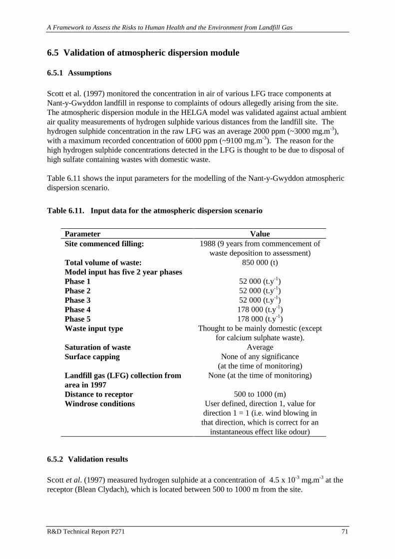
A Framework to Assess the Risks to Human Health and the Environment from Landfill Gas
R&D Technical Report P271 71
6.5 Validation of atmospheric dispersion module
6.5.1 Assumptions
Scott et al. (1997) monitored the concentration in air of various LFG trace components atNant-y-Gwyddon landfill in response to complaints of odours allegedly arising from the site.The atmospheric dispersion module in the HELGA model was validated against actual ambientair quality measurements of hydrogen sulphide various distances from the landfill site. Thehydrogen sulphide concentration in the raw LFG was an average 2000 ppm (~3000 mg.m-3),with a maximum recorded concentration of 6000 ppm (~9100 mg.m-3). The reason for thehigh hydrogen sulphide concentrations detected in the LFG is thought to be due to disposal ofhigh sulfate containing wastes with domestic waste.
Table 6.11 shows the input parameters for the modelling of the Nant-y-Gwyddon atmosphericdispersion scenario.
Table 6.11. Input data for the atmospheric dispersion scenario
Parameter ValueSite commenced filling: 1988 (9 years from commencement of
waste deposition to assessment)Total volume of waste: 850 000 (t)Model input has five 2 year phasesPhase 1 52 000 (t.y-1)Phase 2 52 000 (t.y-1)Phase 3 52 000 (t.y-1)Phase 4 178 000 (t.y-1)Phase 5 178 000 (t.y-1)Waste input type Thought to be mainly domestic (except
for calcium sulphate waste).Saturation of waste AverageSurface capping None of any significance
(at the time of monitoring)Landfill gas (LFG) collection fromarea in 1997
None (at the time of monitoring)
Distance to receptor 500 to 1000 (m)Windrose conditions User defined, direction 1, value for
direction 1 = 1 (i.e. wind blowing inthat direction, which is correct for an
instantaneous effect like odour)
6.5.2 Validation results
Scott et al. (1997) measured hydrogen sulphide at a concentration of 4.5 x 10⁻³ mg.m-3 at thereceptor (Blean Clydach), which is located between 500 to 1000 m from the site.
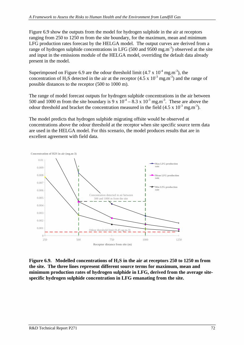
A Framework to Assess the Risks to Human Health and the Environment from Landfill Gas
R&D Technical Report P271 72
Figure 6.9 show the outputs from the model for hydrogen sulphide in the air at receptorsranging from 250 to 1250 m from the site boundary, for the maximum, mean and minimumLFG production rates forecast by the HELGA model. The output curves are derived from arange of hydrogen sulphide concentrations in LFG (500 and 9500 mg.m-3) observed at the siteand input in the emissions module of the HELGA model, overriding the default data alreadypresent in the model.
Superimposed on Figure 6.9 are the odour threshold limit (4.7 x 10⁻⁴ mg.m-3), theconcentration of H2S detected in the air at the receptor (4.5 x 10⁻³ mg.m-3) and the range ofpossible distances to the receptor (500 to 1000 m).
The range of model forecast outputs for hydrogen sulphide concentrations in the air between500 and 1000 m from the site boundary is 9 x 10⁻⁴ – 8.3 x 10⁻³ mg.m-3. These are above theodour threshold and bracket the concentration measured in the field (4.5 x 10⁻³ mg.m-3).
The model predicts that hydrogen sulphide migrating offsite would be observed atconcentrations above the odour threshold at the receptor when site specific source term dataare used in the HELGA model. For this scenario, the model produces results that are inexcellent agreement with field data.
0
0.001
0.002
0.003
0.004
0.005
0.006
0.007
0.008
0.009
0.01
250 500 750 1000 1250
Receptor distance from site (m)
Max LFG productionrate
Mean LFG productionrate
Min LFG productionrate
Odour threshold limit (0.45 ug.m-3)
Concentration detected in air between500 and 1000 m from the site
Concentration of H2S in air (mg.m-3)
Figure 6.9. Modelled concentrations of H2S in the air at receptors 250 to 1250 m fromthe site. The three lines represent different source terms for maximum, mean andminimum production rates of hydrogen sulphide in LFG, derived from the average site-specific hydrogen sulphide concentration in LFG emanating from the site.

A Framework to Assess the Risks to Human Health and the Environment from Landfill Gas
R&D Technical Report P271 73
6.6 Validation of Lateral Migration
6.6.1 Assumptions
The lateral migration module has been validated against data from Foxhall landfill site, whichhas been well characterised and monitored for VOCs in a lateral emission plume from part ofthe site (Ward et al., 1996). Table 6.12 shows the module input parameters for this scenario.
Table 6.12. Input data for the lateral migration scenario.
Parameter ValueGround porosity 40 % (assume the geology is sandy
gravel, taken from published data)Assume at field capacity 10 % (assume a well drained
unsaturated material)Ground saturation 25 %VOC concentrations in LFG model defaults have been used
Table 6.13 shows the measured concentration of three VOCs detected in the ground at 5mdepth, 40m away from the site.
Table 6.13. VOC concentrations at 5m depth, 40 m from the site boundary.
VOC Maximumconcentration inLFG at the site
boundary (ppm)
Measuredconcentrations at40 m offsite (ppm)
Vinyl chloride 4.25 15.4Dichlorodifluromethane 0 13.7Chlorodifluromethane 11.54 3
6.6.2 Model outputs
Figures 6.10 - 6.12 show the range of model forecasts for concentrations of VOCs at 40mfrom the site boundary (shaded box), with the detected concentration superimposed (blackcross) for the three VOCs considered: vinyl chloride, dichlorodifluromethane andchlorodifluoro-methane. The range of concentrations calculated in the model bracket theconcentrations detected in the field investigation.
The lateral dispersion module operates outside the probabilistic framework, but a range ofVOC concentrations has been used to determine the model forecast range. The VOCconcentrations at 40 m are derived from the range of VOC concentrations in LFG provided asmodel defaults before the plume migrates from the site. No biochemical or chemical reactionsare simulated during migration, which is simulated as a diffusion-only system. The results
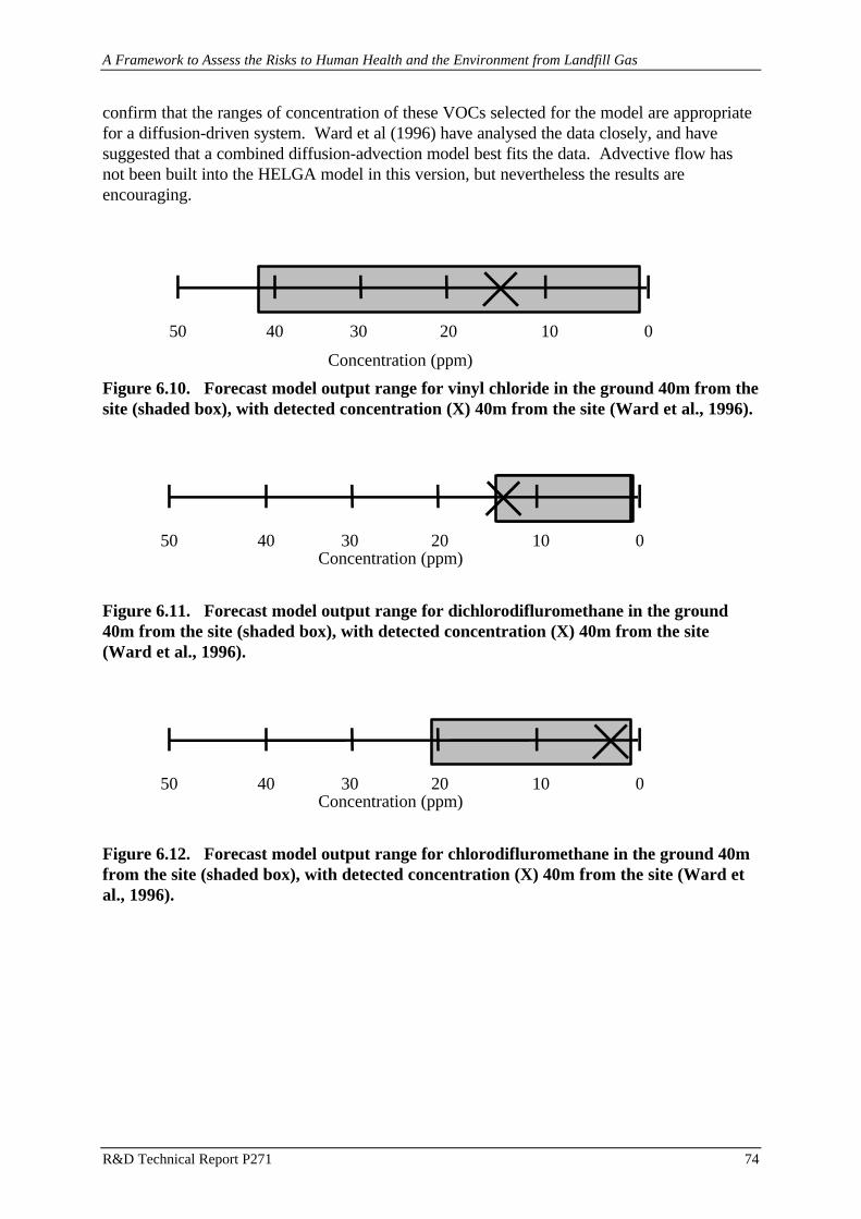
A Framework to Assess the Risks to Human Health and the Environment from Landfill Gas
R&D Technical Report P271 74
confirm that the ranges of concentration of these VOCs selected for the model are appropriatefor a diffusion-driven system. Ward et al (1996) have analysed the data closely, and havesuggested that a combined diffusion-advection model best fits the data. Advective flow hasnot been built into the HELGA model in this version, but nevertheless the results areencouraging.
Figure 6.10. Forecast model output range for vinyl chloride in the ground 40m from thesite (shaded box), with detected concentration (X) 40m from the site (Ward et al., 1996).
Figure 6.11. Forecast model output range for dichlorodifluromethane in the ground40m from the site (shaded box), with detected concentration (X) 40m from the site(Ward et al., 1996).
Figure 6.12. Forecast model output range for chlorodifluromethane in the ground 40mfrom the site (shaded box), with detected concentration (X) 40m from the site (Ward etal., 1996).
50 30 20 10 040Concentration (ppm)
50 30 20 10 040Concentration (ppm)
50
Concentration (ppm)
30 20 10 040

A Framework to Assess the Risks to Human Health and the Environment from Landfill Gas
R&D Technical Report P271 75
6.7 Conclusions from validation tests
6.7.1 Comparison with observations
The findings of the validation tests performed on the HELGA model are encouraging. Not onlydo the key modules produce forecasts which are generally in accordance with fieldobservations, but they do so when driven by a relatively small data requirement. This smalldata requirement is important.
The HELGA model was conceived for use in the planning of landfill gas management for new-build landfills, but could be equally effective when applied to existing sites for landfill gashealth and environmental risk assessments. In both instances, the availability of reliable datawith which to drive the model has a direct effect on the forecasting capability of the decisiontool. For many existing landfill sites, and certainly for new build landfills, much data will bebest estimates, or model defaults. It is encouraging to observe that when data are scarce ornon-existent, the forecast range of results from the HELGA model, using model default data,overlap with actual site measurements.
6.7.2 Uncertainties and deficiencies in the model
As the source-term module determines the amount of landfill gas produced, and the rate atwhich this amount is generated, the user should acquire as much site-specific waste and landfilldesign data as is available.
Model default values for VOCs are acceptable for emissions, but the database for trace landfillgas components and VOCs would benefit from more data to determine the probability densityfunctions for these species. This will be essential for when the model is coded as a free-standing probabilistic decision tool.
Waste composition data for commercial and industrial waste streams are still poorlycharacterised today, so the ability to forecast emissions from landfills which accept thesewastes is limited by the lack of data.
The steady state lateral migration model uses only diffusion driven flow. Advective flow, tosimulate flow in fractures, could be added to enhance the model’s forecasting abilities.
The migration event module is not as sophisticated as other modules in the model, and doesnot sit comfortably within a probabilistic decision tool. We would suggest that this module isomitted from future developments of the code.
A Framework to Assess the Risks to Human Health and the Environment from Landfill Gas
R&D Technical Report P271 76
7. LFG EMISSIONS MANAGEMENT OPTIONS
7.1 Introduction
The primary purpose of the HELGA decision tool is to aid the implementation of appropriatelandfill gas management methods at the planning and subsequent stages of operation of amodern-day landfill. In order to demonstrate the flexibility of the HELGA model to do this,four scenarios have been simulated which demonstrate the effect of different cap designs on alandfill site, and the effect of different landfill gas management options employed on the site.
All the scenarios considered apply to a notional site in eastern England accepting 5Mthousehold waste over a ten-year period. The scenarios considered are as follows:
• Scenario 1. A minimal soil cap of 0.3m thickness, and no other gas controls.• Scenario 2. A 1m clay cap with 0.8m soil cover, and no other gas controls.• Scenario 3. As Scenario 2 with the addition of gas collection and flaring.• Scenario 4. As Scenario 2 with the addition of gas collection, flaring and gas utilisation. For each scenario, we have considered the effect on emissions 12 years after the start of siteoperations, i.e. 2 years after completion of filling, when gas generation and control will be animportant environmental concern. HELGA has the ability to produce a vast array of usefulinformation for each year after commencement of filling (up to 150 years after start oflandfilling), for landfill gas and each VOC on the database. The choice of 2 years aftercompletion of filling allows for a like-for-like comparison between the scenarios. We havechosen to compare the following indicative parameters for each scenario.
• Gas generation.• Carbon dioxide and methane generation rate.• Landfill gas migration through the cap and liner.• Methane oxidation in the cap.
• VOC emissions through the cap.• Comparison of emission rates of hydrogen sulphide, methanethiol, benzene, vinyl
chloride, dioxins, hydrogen chloride and NOx.
• Site Worker Exposure.• Comparison of air concentrations on-site with LTELs for hydrogen sulphide,
methanethiol, benzene, vinyl chloride, dioxins, hydrogen chloride and NOx.
• Offsite Inhalation Exposure.• The scenarios consider a suspended floor single storey house located 200m WSW
from the landfill site.• Indoor and outdoor concentrations of VOCs hydrogen sulphide, methanethiol,
benzene, vinyl chloride, dioxins, hydrogen chloride and NOx are evaluated.• Average annual exposure to the maximally exposed individuals are determined.

A Framework to Assess the Risks to Human Health and the Environment from Landfill Gas
R&D Technical Report P271 77
• Comparison is made to the inhalation exposure limit (if any).
Table 7.1 below gives all the base case simulation data that remain constant throughout thefour model scenarios. Table 7.2 sets out the variables for the four scenarios compared.
Table 7.1 Simulation data common to all scenarios
Parameter Value Units of measurementSource TermWaste composition 100% domestic %Fill rate 500,000 tonnes per yearFill period 10 yearsSite capacity/void space 5,000,000 m3
Landfill gas composition 50% methane %Adsorbtive capacity of waste 10 %Effective waste porosity 10 %Hydraulic conductivity of waste 1 x 10⁻⁶ m s-1
Waste conductivity to gas 9.8 x 101 m s-1
Liner and ground conditionsSurface area 25 HaSite dimensions 500 x 500 x 20 mBasal clay liner thickness 1 mGas conductivity of basal liner 9.8 x 10⁻⁵ m s-1
Soil porosity (for lateral migration) 0.1 unitless (i.e. 10%)Ground saturation 10 %Leachate recirculation none
Receptor detailsDistance to receptor 250 mHouse perimeter 35 mGround floor area 75 m2
Area of windows and doors 20 m2
Height of living space 2.5 mHeight of suspended floor area/cellar 0.5 mArea of walls in living space 320 m2
Area of walls in suspended floor area/cellar 186 m2
Receptor target height above ground level 2 mPollutant/VOC release height 0 mPollutant/VOC characteristics non-reactiveWind rose location east coastVector of property from landfill site WSWYear of interest 12 years after site
commenced filling
Note: Many of the parameters listed here which are not site specific can be used as defaults in the absence ofsite-specific data.

A Framework to Assess the Risks to Human Health and the Environment from Landfill Gas
R&D Technical Report P271 78
Table 7.2 Key variables in the four scenarios
Parameter Scenario 1:Sandy soilcap, nogascollection
Scenario 2:Clay cap,no gascollection
Scenario 3:Clay capwith gasflaring
Scenario 4:Clay capwith gasutilisation
Units ofmeasurement
Cap detailsSoil Thickness 0.3 0.8 0.8 0.8 mClay thickness 0.0 1.0 1.0 1.0 mThickness of layerwith lowest gasconductivity
0.3 1.0 1.0 1.0 m
Gas conductivityof this layer
1 x 10² 9.8 x 10⁻⁵ 9.8 x 10⁻⁵ 9.8 x 10⁻⁵ m s-1
Infiltration 100 50 50 50 mm y-1
Leachate head 6 1 1 1 mSummary of sitewater balanceconditions
average dry dry dryCalculatedfrom data oninfiltration andleachate head
Gas collection system details
Flare details
Utilisation scheme details

A Framework to Assess the Risks to Human Health and the Environment from Landfill Gas
R&D Technical Report P271 79
It should be noted that the database of VOCs and trace gases used to derive the ranges ofemissions reported below is not complete, although it does comprise an accurate record of theUK data available at the time of construction of the HELGA model. In order to provide evenmore confidence in the HELGA forecasts, new data should be added to the database, as itbecomes available.
7.2 Results of gas generation simulations
Gas generation, migration and methane oxidation rates for the four scenarios are shown inTable 7.3 below.
7.2.1 Gas generation
Results for the mean (50th percentile) and one standard deviation either side of the mean(5th percentile and 95th percentile) are given for each of the four scenarios. These data show awide range of potential gas generation rates possible for the quantities of waste emplaced.This is because the relatively poorly understood mechanisms of gas generation, and other site-specific factors, have to be represented in a model of this nature by probability densityfunctions, or their equivalents.
Table 7.3 shows the total quantities of landfill gas produced, and the rates of landfill gasproduction per year. The landfill gas generation profile is identical for Scenarios 2-4. This isbecause these three scenarios had the same water infiltration and waste degradation conditions,and were calculated by the model to be analogous to a ‘dry’ site (the model allows dry,average and wet sites to be simulated, and will also calculate this from infiltration and leachatehead data). The landfill gas generation profile for Scenario 1 shows higher gas generationrates in the early years of the site’s gas profile. Infiltration and water content of the waste is akey parameter in regulating the rate of decomposition of landfilled waste, and becauseinfiltration through the soil cap will be higher than that for a clay cap, the consequent rate ofgas generation was raised to that of ‘average’ moisture content. Figure 7.1 shows the gasproduction curves for Scenario 1, and Figure 7.2 for the other three scenarios.
7.2.2 Potential for gas migration through cap and liner
The potential for gas migration through the cap or liner is proportional to the thickness andpermeability of each liner. Table 7.3 shows that Scenario 1, with the soil cap, and no otherforms of gas control, performs worst of all, with all gas generated migrating through the cap.Scenario 2, with a 1m clay cap, also loses most of the gas generated through the covermaterials. Only Scenarios 3 and 4, where gas collection and flaring/utilisation is simulated,reduces surface emissions significantly, compared with the base case.
In these examples, Scenario 4 shows most reduction in emissions. This need not be the case,however. The absolute value of emissions reduction in Scenarios 3 and 4 for any particularyear (note that this is year 12) will depend upon the sizing of flare and/or utilisation schemeemployed on the site. This sizing must be done by examining the base case gas generation
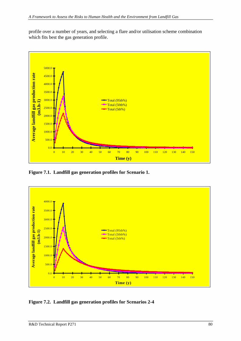
A Framework to Assess the Risks to Human Health and the Environment from Landfill Gas
R&D Technical Report P271 80
profile over a number of years, and selecting a flare and/or utilisation scheme combinationwhich fits best the gas generation profile.
0.0
500.0
1000.0
1500.0
2000.0
2500.0
3000.0
3500.0
4000.0
4500.0
5000.0
0 10 20 30 40 50 60 70 80 90 100 110 120 130 140 150
Time (y)
Ave
rage
land
fill
gas
prod
ucti
on r
ate
(m3.
h-1) Total (95th%)
Total (50th%)Total (5th%)
Figure 7.1. Landfill gas generation profiles for Scenario 1.
0.0
500.0
1000.0
1500.0
2000.0
2500.0
3000.0
3500.0
4000.0
0 10 20 30 40 50 60 70 80 90 100 110 120 130 140 150
Time (y)
Ave
rage
land
fill
gas
prod
ucti
on r
ate
(m3.
h-1) Total (95th%)Total (50th%)Total (5th%)
Figure 7.2. Landfill gas generation profiles for Scenarios 2-4
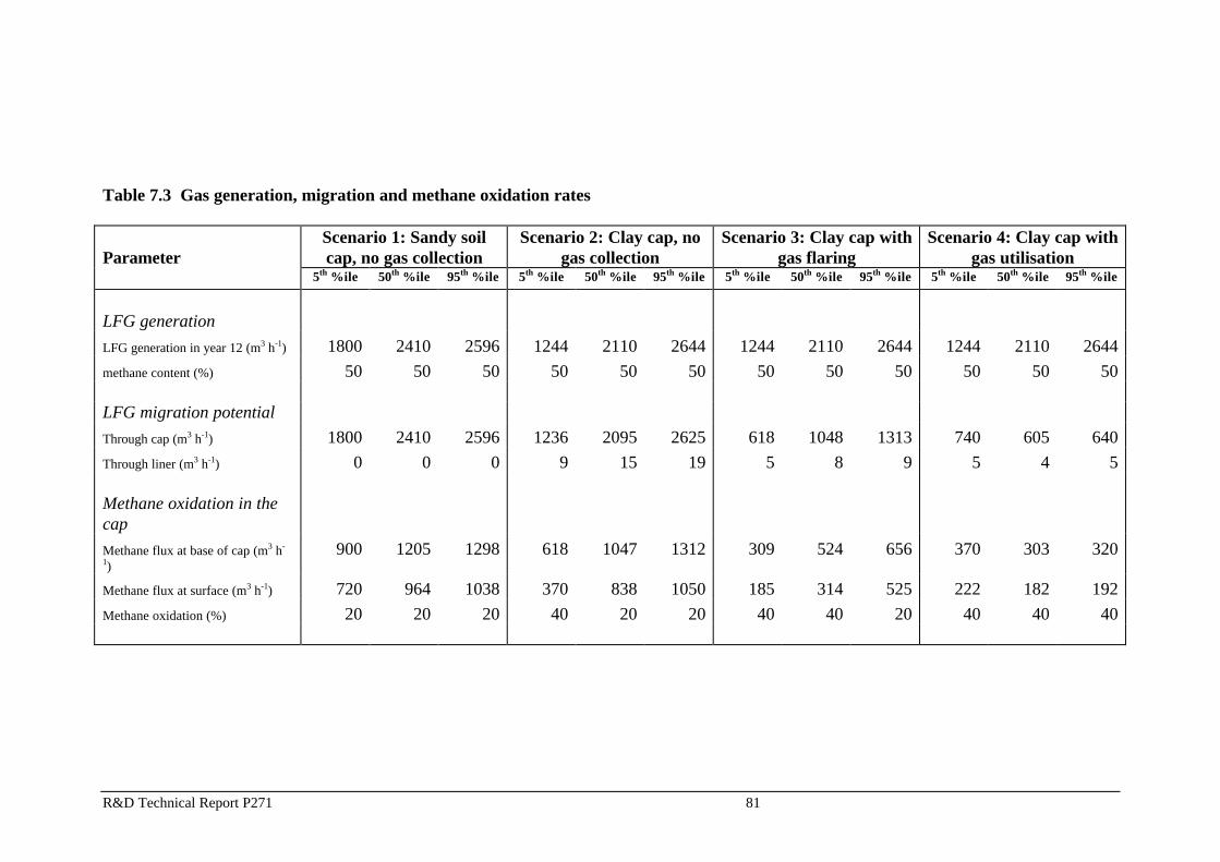
R&D Technical Report P271 81
Table 7.3 Gas generation, migration and methane oxidation rates
ParameterScenario 1: Sandy soilcap, no gas collection
Scenario 2: Clay cap, nogas collection
Scenario 3: Clay cap withgas flaring
Scenario 4: Clay cap withgas utilisation
5th %ile 50th %ile 95th %ile 5th %ile 50th %ile 95th %ile 5th %ile 50th %ile 95th %ile 5th %ile 50th %ile 95th %ile
LFG generation
LFG generation in year 12 (m3 h-1) 1800 2410 2596 1244 2110 2644 1244 2110 2644 1244 2110 2644
methane content (%) 50 50 50 50 50 50 50 50 50 50 50 50
LFG migration potential
Through cap (m3 h-1) 1800 2410 2596 1236 2095 2625 618 1048 1313 740 605 640
Through liner (m3 h-1) 0 0 0 9 15 19 5 8 9 5 4 5
Methane oxidation in thecap
Methane flux at base of cap (m3 h-
1)900 1205 1298 618 1047 1312 309 524 656 370 303 320
Methane flux at surface (m3 h-1) 720 964 1038 370 838 1050 185 314 525 222 182 192
Methane oxidation (%) 20 20 20 40 20 20 40 40 20 40 40 40

A Framework to Assess the Risks to Human Health and the Environment from Landfill Gas
R&D Technical Report P271 82
7.2.3 Methane oxidation in the cap
The degree of methane oxidation in the cap is a function of the rate of transmission of landfillgas through the cap thickness, which is driven by the rate of gas generation (after collection ofa fraction of the gas for flaring and/or utilisation. If the rate of gas generation is sufficientlyhigh that the movement of gas through the cap takes less than one second (an arbitrary value,but one which appears to work well and mimic observed behaviour), then the degree ofmethane oxidation observed is 20%. If gas movement takes longer than one second, then thedegree of methane oxidation observed is 40%. These values of 20% and 40% are againarbitrary, as there are no data to confirm these values, but again, the pattern of behaviour andthe results produced agree well with observed, but unquantified, gas behaviour.
The scenarios in Table 7.3 show a steady increase in the likelihood of high levels of methaneoxidation in the capping layers as the quantity of landfill gas which is collected and flared orotherwise utilised increases. This means that the more gas diverted to flare or utilisation, awayfrom the cap, the lower the ‘loading’ on the cap, and the higher the opportunity for methaneoxidising bacteria to cope with the flux of uncontrolled gas.
These figures will also impact on global environmental burdens (global warming potential andozone depleting potential. See section 7.3 below.
7.3 Global environmental burdens
The HELGA model takes the emissions data and calculates the global warming potential(GWP) (in tonne equivalents of carbon dioxide), and the ozone depletion potential (ODP) (intonne equivalents of fluoro-trichloromethane (CCl3F)). The results of the simulations (for the50th percentile gas generation rates) are shown in Table 7.4.
These results clearly show that for any given site that generates landfill gas, the effects ofcapping, flaring and gas utilisation progressively reduce the global environmental burden dueto that particular site. Obviously, these figures only apply to year 12. Over the site’s entirelife, a reduction in GWP and ODP of over 70%, compared to the base case, will not beattained, as flaring and gas utilisation are only appropriate over the most productive phases ofgas generation. However, since flaring and utilisation can manage the bulk of the gas, thebenefits to the environment of these landfill gas management systems are obvious.

A Framework to Assess the Risks to Human Health and the Environment from Landfill Gas
R&D Technical Report P271 83
Table 7.4. Global environmental burdens
Scenario 1:Sandy soil cap,
no gascollection
Scenario 2:Clay cap, nogas collection
Scenario 3:Clay cap with
gas flaring
Scenario 4:Clay cap withgas utilisation
GWP (tonnesequivalent CO2)
130,000 113,000 47,000 30,500
Percentagereduction frombase case
0 13 64 77
ODP (tonnesequivalent CCl3F)
0.35 0.30 0.15 0.09
Percentagereduction frombase case
0 14 57 74
Note: The base case is Scenario 1
7.4 VOC emissions
VOC and trace gas emissions through the cap, flare and utilisation scheme have beencalculated for the following substances:
• benzene• hydrogen sulphide• methanethiol• vinyl chloride• dioxins• hydrogen chloride• nitrogen oxides The HELGA model generates mean, minimum and maximum forecast values for each of the5th, 50th and 95th percentile gas generation rates. The data given in Table 7.5 below werederived using the 50th percentile gas generation rate. Not all the compounds listed above arereleased via each emission pathway, and it should be noted that the quantities of VOCsreleased via each pathway are directly proportional to the volumes of landfill gas emitted viaeach pathway. All dioxin forecasts should be treated with great care, as only one data value forsurface emissions, flare and engine emissions exist in the HELGA database. The data in Table 7.5 only show the total site surface emissions, and emissions from the flareor utilisation scheme. They should not be interpreted as exposures. Site worker exposure andoffsite inhalation exposures are discussed in Sections 7.5 and 7.6 respectively.
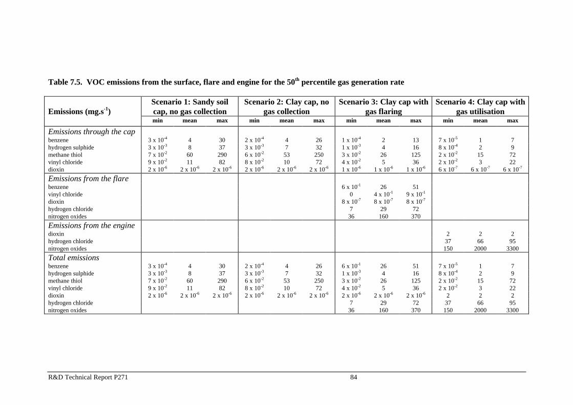
R&D Technical Report P271 84
Table 7.5. VOC emissions from the surface, flare and engine for the 50th percentile gas generation rate
Emissions (mg.s-1)
Scenario 1: Sandy soilcap, no gas collection
Scenario 2: Clay cap, nogas collection
Scenario 3: Clay cap withgas flaring
Scenario 4: Clay cap withgas utilisation
min mean max min mean max min mean max min mean max
Emissions through the cap benzene 3 x 10⁻⁴ 4 30 2 x 10⁻⁴ 4 26 1 x 10⁻⁴ 2 13 7 x 10⁻⁵ 1 7 hydrogen sulphide 3 x 10⁻³ 8 37 3 x 10⁻³ 7 32 1 x 10⁻³ 4 16 8 x 10⁻⁴ 2 9 methane thiol 7 x 10⁻² 60 290 6 x 10⁻² 53 250 3 x 10⁻² 26 125 2 x 10⁻² 15 72 vinyl chloride 9 x 10⁻² 11 82 8 x 10⁻² 10 72 4 x 10⁻² 5 36 2 x 10⁻² 3 22 dioxin 2 x 10⁻⁶ 2 x 10⁻⁶ 2 x 10⁻⁶ 2 x 10⁻⁶ 2 x 10⁻⁶ 2 x 10⁻⁶ 1 x 10⁻⁶ 1 x 10⁻⁶ 1 x 10⁻⁶ 6 x 10⁻⁷ 6 x 10⁻⁷ 6 x 10⁻⁷
Emissions from the flare benzene 6 x 10⁻¹ 26 51 vinyl chloride 0 4 x 10⁻¹ 9 x 10⁻¹ dioxin 8 x 10⁻⁷ 8 x 10⁻⁷ 8 x 10⁻⁷ hydrogen chloride 7 29 72 nitrogen oxides 36 160 370 Emissions from the engine dioxin 2 2 2 hydrogen chloride 37 66 95 nitrogen oxides 150 2000 3300
Total emissions benzene 3 x 10⁻⁴ 4 30 2 x 10⁻⁴ 4 26 6 x 10⁻¹ 26 51 7 x 10⁻⁵ 1 7 hydrogen sulphide 3 x 10⁻³ 8 37 3 x 10⁻³ 7 32 1 x 10⁻³ 4 16 8 x 10⁻⁴ 2 9 methane thiol 7 x 10⁻² 60 290 6 x 10⁻² 53 250 3 x 10⁻² 26 125 2 x 10⁻² 15 72 vinyl chloride 9 x 10⁻² 11 82 8 x 10⁻² 10 72 4 x 10⁻² 5 36 2 x 10⁻² 3 22 dioxin 2 x 10⁻⁶ 2 x 10⁻⁶ 2 x 10⁻⁶ 2 x 10⁻⁶ 2 x 10⁻⁶ 2 x 10⁻⁶ 2 x 10⁻⁶ 2 x 10⁻⁶ 2 x 10⁻⁶ 2 2 2 hydrogen chloride 7 29 72 37 66 95 nitrogen oxides 36 160 370 150 2000 3300

A Framework to Assess the Risks to Human Health and the Environment from Landfill Gas
R&D Technical Report P271 85
What these data do show is the relationship between emissions due to natural landfill gasemissions, the effect of flaring or gas utilisation on these natural emissions, and the additionalcombustion products resulting from flaring or gas utilisation. The emissions data show the following.
• Increasing the level of gas collection and flaring or utilisation reduces the uncontrolledsurface emissions of VOCs proportionately.
• The available data for VOC emissions show wide uncertainty ranges (or wide variations inlandfill gas trace gas compositions) for some components. The forecast emissions ofbenzene, for example, could vary over six orders of magnitude. Additional VOC emissionsmeasurements should be made to drive this model if reliable forecasts are to be made.
• Some results will be unreliable because of the lack of sufficient monitoring data (e.g.dioxins).
• Flaring or combustion destroys compounds to different degrees. Hydrogen sulphide andmethanethiol, for example, have not been recorded in significant concentrations from flareor gas engine emissions. The dioxin content of flared landfill gas is comparable to theunflared gas.
• Some flare or gas engine combustion products (hydrogen chloride, nitrogen oxides) occurin much higher concentrations that the landfill trace gases or VOCs represented in themodel. This is because they are derived from combustion of many other VOCs notrepresented in the model, and more than one atom of the combustion products are producedfrom each VOC molecule, i.e. there are more of them per cubic metre than the VOCs theyare derived from.
7.5 Results of site worker exposure simulations
Comparisons of the concentrations in air on site of the selected compounds with long-termexposure limits (LTELs) are made in Table 7.6. All exposure concentrations are very low, andwhere LTELs exist, are below the LTEL by between 4 and 5 orders of magnitude.
It is clear from the simulations that the use of flaring and/or gas utilisation diverts VOCs fromdirect emission through the cap, and these combustion processes destroy a fraction of theVOCs sent to the flare or gas engine, thereby reducing the total emissions of landfill-sourcedVOCs released. However, combustion products from the gas engines are in significantlyhigher concentrations than the naturally emitted landfill VOCs.
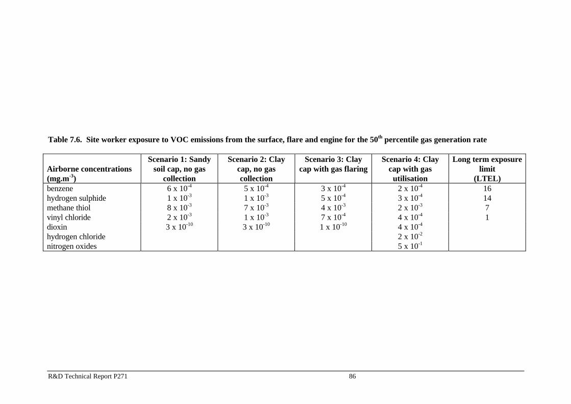
R&D Technical Report P271 86
Table 7.6. Site worker exposure to VOC emissions from the surface, flare and engine for the 50th percentile gas generation rate
Airborne concentrations(mg.m-3)
Scenario 1: Sandysoil cap, no gas
collection
Scenario 2: Claycap, no gascollection
Scenario 3: Claycap with gas flaring
Scenario 4: Claycap with gas
utilisation
Long term exposurelimit
(LTEL)benzene 6 x 10⁻⁴ 5 x 10⁻⁴ 3 x 10⁻⁴ 2 x 10⁻⁴ 16hydrogen sulphide 1 x 10⁻³ 1 x 10⁻³ 5 x 10⁻⁴ 3 x 10⁻⁴ 14methane thiol 8 x 10⁻³ 7 x 10⁻³ 4 x 10⁻³ 2 x 10⁻³ 7vinyl chloride 2 x 10⁻³ 1 x 10⁻³ 7 x 10⁻⁴ 4 x 10⁻⁴ 1dioxin 3 x 10⁻¹⁰ 3 x 10⁻¹⁰ 1 x 10⁻¹⁰ 4 x 10⁻⁴
hydrogen chloride 2 x 10⁻²
nitrogen oxides 5 x 10⁻¹

A Framework to Assess the Risks to Human Health and the Environment from Landfill Gas
R&D Technical Report P271 87
7.6 Results of offsite inhalation exposure simulations
Offsite inhalation exposure here considers the average annual exposure, from indoor andoutdoor exposure, for the most highly exposed individual living in a property with a suspendedfloor 250m from the landfill. The wind rose for eastern England has been used, and theproperty is downwind of the prevailing wind direction. The results of these simulations aregiven in Table 7.7.
Table 7.7. Offsite inhalation exposure scenarios
Scenario/VOCConcentrationoutdoors (mg.m3)
Concentrationindoors (mg.m3)
Average annualexposure (mg.y--1)
Is inhalationexposure limitexceeded?
Scenario 1: sandy soil cap, no gas collectionBenzene 2 x 10⁻⁶ 0 4 x 10⁻³Hydrogen sulphide 4 x 10⁻⁶ 7 x 10⁻⁷ 1 x 10⁻² noMethanethiol 3 x 10⁻⁵ 6 x 10⁻⁶ 9 x 10⁻²Vinyl chloride 5 x 10⁻⁶ 0 9 x 10⁻³Dioxins 1 x 10-12 0 2 x 10⁻⁹
Scenario 2: clay cap, no gas collectionBenzene 2 x 10⁻⁶ 0 3 x 10⁻³Hydrogen sulphide 3 x 10⁻⁶ 7 x 10⁻⁷ 1 x 10⁻² noMethanethiol 2 x 10⁻⁵ 6 x 10⁻⁶ 8 x 10⁻²Vinyl chloride 4 x 10⁻⁶ 0 8 x 10⁻³Dioxins 9 x 10-13 0 2 x 10⁻⁹
Scenario 3: Clay cap with gas flaringBenzene 9 x 10⁻⁷ 0 2 x 10⁻³Hydrogen sulphide 2 x 10⁻⁶ 7 x 10⁻⁷ 8 x 10⁻³ noMethanethiol 1 x 10⁻⁵ 6 x 10⁻⁶ 6 x 10⁻²Vinyl chloride 2 x 10⁻⁶ 0 4 x 10⁻³Dioxins 4 x 10-13 0 8 x 10⁻¹⁰
Scenario 4: clay cap with gas utilisationBenzene 5 x 10⁻⁷ 0 9 x 10⁻⁴Hydrogen sulphide 9 x 10⁻⁷ 7 x 10⁻⁷ 7 x 10⁻³ noMethanethiol 7 x 10⁻⁶ 6 x 10⁻⁶ 5 x 10⁻²Vinyl chloride 1 x 10⁻⁶ 0 2 x 10⁻³Dioxins 2 x 10⁻⁶ 0 4 x 10⁻³Hydrogen chloride 9 x 10⁻⁵ 0 2 x 10⁻¹ noNitrogen oxides 3 x 10⁻³ 0 5
These results mimic the pattern shown for workers above, but because of distance from thelandfill, the outdoor concentrations are typically two to three orders of magnitude lower thanthose over the site. It is unlikely that any exposures will exceed the inhalation exposure limit.
A Framework to Assess the Risks to Human Health and the Environment from Landfill Gas
R&D Technical Report P271 88
Again, it is clear from the simulations that the use of flaring and/or gas utilisation diverts VOCsfrom direct emission through the cap, and both flaring and gas utilisation plant destroy afraction of the VOCs, thereby reducing the human exposure to landfill-sourced VOCs.However, combustion products from the gas engines are in significantly higher concentrationsthan the naturally emitted landfill VOCs. The absence of inhalation exposure limits for manysubstances makes further interpretation of the values difficult, but it is obvious that emissionsare of a low order.
7.7 Conclusions
The aim of constructing the four scenarios set out above was to demonstrate the effect ofchanging cap type and employing gas collection, flaring and utilisation as landfill gasmanagement techniques. To date there has been little in the way of quantitative measurementson the need or effectiveness of landfill gas management techniques. Whilst the data in thesescenarios apply to a notional landfill site, the main findings will apply to all landfills whichaccept biodegradable waste.
These findings are summarised as follows.
• The gas generation rate for Scenario 1, the sandy soil capped site, was higher than the ratefor any of the clay capped site scenarios (Scenarios 2-4). This was due to a combination ofa higher rate of rainfall infiltration into the site, and a higher standing head of leachatewithin the site. This increased the net water content of the waste, and therefore acceleratingdecomposition of the waste.
• The stepwise effect of improving cap quality on the site, from a soil cap (Scenario 1) to aclay cap (Scenario 2), introducing gas collection and flaring (Scenario 3) or gas utilisation(Scenario 4) has the following benefits:
• surface emissions are reduced; and• as more gas is collected and flared or utilised, the fraction of landfill gas remaining
which can undergo methane oxidation increases, because the net methane flux isreduced.
• The global warming potential (GWP) and ozone depleting potential (ODP) results clearlyshow that for any given site which generates landfill gas, the effects of capping, flaring andgas utilisation progressively reduce the global environmental burden due to that particularsite. In year 12 of the site’s life, a reduction in GWP and ODP of over 70% could beattained. This percentage will not be sustained over the site’s entire life, but since the bulkof the landfill gas generated within the site can be managed by flaring and utilisation, thebenefits to the environment of these landfill gas management systems are obvious.
• VOC emissions from the surface of the site are proportional to the rate of bulk landfill gasemissions, and so the quantities of VOCs emitted from the landfill are reduced by theaddition of a clay cap (Scenario 2), introduction of gas collection and flaring (Scenario 3) orgas utilisation (Scenario 4).

A Framework to Assess the Risks to Human Health and the Environment from Landfill Gas
R&D Technical Report P271 89
• Site worker exposures to landfill gas VOC emissions are reduced by flaring or gasutilisation (Scenarios 3 and 4). The emissions of all trace gas components are well belowpermitted levels of exposure (where exposure limits exist) in all scenarios, althoughemissions from landfill gas engines are, as would be expected, in higher concentrations thanthe uncollected landfill gas emitted from the site.
• Maximally exposed individual exposures to landfill gas VOC emissions are also reduced byflaring or gas utilisation (Scenarios 3 and 4). Although combustion products are producedfrom the landfill gas engine, the emissions of all trace gas components are well belowpermitted levels of exposure (where exposure limits exist) in all scenarios.
On balance, taking into account uncertainties and omissions of data from the landfill gas andVOC database, the scenarios modelled offer the following interpretation for gas managementat this notional landfill site, which can be applied to the majority of modern landfills.
The provision of an engineered cap on a landfill has been shown to reduce annual landfill gasemissions, but this is due to changes in waste degradation rates rather than positivelydestroying trace gases or VOCs.
However, landfill gas flaring and/or gas utilisation provide positive steps to reducing trace gasand VOC emissions, by collecting a significant fraction of the landfill gas generated by anindividual landfill site, and destroying a high percentage of the bulk and trace landfill gasconstituents in the combustion process. These combustion processes are not without theirown environmental burdens, and low temperature combustion processes, particularly thosefrom landfill gas engines, generate higher concentrations of emission by-products such ashydrogen chloride and nitrogen oxides.
Landfill gas flaring and/or gas utilisation provides significant global environmental protection,as these gas management options reduce the quantities of landfill gas emitted to atmosphere,and consequently reduce the landfill site’s individual GWP and ODP.
The interpretation of the environmental impact of landfill gas flaring and/or gas utilisation interms of local human health effects is difficult to quantify, as destruction of some trace gasesand VOCs results in formation of different combustion products. Exposure limit standards orhealth risk data are not available for many of the components in landfill gas, so it is difficult todetermine whether these emission products are a significant risk. All the data show that whereexposure limit data are available, the emissions for all scenarios considered do not exceedexposure limits.
A Framework to Assess the Risks to Human Health and the Environment from Landfill Gas
R&D Technical Report P271 90
8. REFERENCES
Agriculture and Food Research Council (1988). A basic study of landfill microbiology andbiochemistry. Department of Energy Renewable Energy Research and DevelopmentProgramme. ETSU Report B1159
Barlaz, M.A., Schaefer D.M. and Ham R.K. (1989) Mass balance analysis of decomposedrefuse in laboratory scale lysimeters. ASCE Journal of Environmental Engineering, 115(6):1088-1102
Barlaz M A, Eleazer W E, Odle S, Xingdong Qian and Yu-Sheng Wang (1996)Biodegradative analysis of municipal solid waste in laboratory-scale landfills. Draft US EPAreport, August 1996.
BBC (1978) The people’s activities and use of time, BBC Audience Research Department.
DoE (1991) The technical aspects of controlled waste management: Field investigations ofmethane oxidation. Report CWM 042/91. Department of the Environment, London, UK.
DoE (1991) Waste Management Paper No 27: Landfill Gas. London HMSO.
DoE (1994) The technical aspects of controlled waste management: National household wasteanalysis project - phase 2, volume 1, report on composition and weight data. Report CWM082/94. Department of the Environment, London, UK
DoE (1994a) The technical aspects of controlled waste management: Optimising methaneoxidation in landfill cover soils. Report CWM 114/94l. Department of the Environment,London, UK
Farquhar G.J and Rovers F.A (1973) Gas production during refuse decomposition. Water, Airand Soil Pollution, 2: 483-493
Ferguson, C. and Marsh, J. (1993) Assessing Human Health Risks from Ingestion ofContaminated Soil, Land Contamination and Reclamation, 1(4): 177-187.
Hoeks J and Oosthoek J (1981) Gaswinning uit afvalstortterreinen. Gas, 101.
ICRP (1994) Human Respiratory Tract Model for Radiological Protection, ICRP Publication66, Annals of ICRP 24 (1-3).
MAFF (1987) Personal communication with Mr Ben Walters, unpublished MAFF data oncritical group food consumption. Ministry of Agriculture, Fisheries and Food, London.
NRPB (1987) Patterns of Building Occupancy for the General Public, E.A. Francis. NRPBMemorandum- M129, National Radiological Protection Board, Didcot, Oxon.
NRPB et al (1995). Methodology for assessing the radiological consequences of routinereleases of radionuclides to the environment. Report EUR 15760. Luxembourg, European

A Framework to Assess the Risks to Human Health and the Environment from Landfill Gas
R&D Technical Report P271 91
Commission.
NRPB (1996) Generalised Habit data for Radiological Assessments, C.A. Robinson. NRPBMemorandum- M636, National Radiological Protection Board, Didcot, Oxon.
Oonk H, Weenk A, Coops O and Luning L (1994) Validation of landfill gas formation models.TNO report 94-315.
Senior, E. (1989). Microbiology of Landfill Sites. CRC Press Inc.
Travis, C.C. and Arms, A.D. (1988) Bioconcentration of organics in beef, milk andvegetation. Environ.Sci. Technol., 22 (3) : 271-274.
UK Working Group on Atmospheric Dispersion (1979). A model for short and medium rangedispersion of radionuclides released to the atmosphere. First report of the Working Group.NRPB-R91. London, HMSO.
UK Working Group on Atmospheric Dispersion (1981). A procedure to include deposition inthe model for short and medium range atmospheric dispersion of radionuclides. Second reportof the Working Group. NRPB-R122. London, HMSO.
USEPA (1988a). Superfund exposure assessment manual. P389-135859. United StatesEnvironmental Protection Agency.
USEPA (1988b). EPA report 540/1-88/001. United States Environmental Protection Agency.
Walters, B. (1995) Do critical groups eat a lot of food all the time, and where does it comefrom? International Symposium on Environmental Impact of Radioactive Releases, Vienna,Austria, IAEA-SM339/189P.
WS Atkins (1997) Methane emissions from different landfill categories. Draft final report tothe Environment Agency. March 1997. Published as R&D Technical Report P233a,Environment Agency, 1999.
Zanten B van and Scheepers M J J (1996) Modelling of landfill gas potentials. Working paperInternational Energy Agency Activity.