a forensic analysis of liquidity and credit risk in ... · pdf filea forensic analysis of...

A Forensic Analysis of Liquidity and Credit Risk inEuropean Sovereign Bond Markets

Jennie Bai, Christian Julliard and Kathy Yuan∗

May 9, 2012

Very Preliminary

Abstract

We study how liquidity and credit risks evolve in European sovereign bond marketssince 2006. We have three sets of findings. First, we find by structural break analysisthat liquidity started to affect sovereign bond yields significantly after the credit crisisof 2008 but has a much smaller effect after the late 2009. That is, the bond spreadvariation during the early stage of the Euro area sovereign bond crisis is mostly dueto liquidity concerns (i.e., flight to liquidity), but during the second stage it is mostlycredit risk driven (flight to quality). Second, we find CDS markets lead bond marketsin price discovery normally but this lead is substantially reduced/reversed during thecrisis stage, indicating that a potential spillover from credit risk to liquidity. Finally,we find through VAR analyses a spillover from the aggregate credit risk premium toeach individual country credit risk premium, a spillover effect from the credit riskpremium of each country to its liquidity risk. We do not find, however, a feedbackfrom the aggregate or individual country’s liquidity risk to a country’s liquidity risk.These findings indicate that even though liquidity risk may be related to the creditrisk premium of a country, the European sovereign bond crisis is a contagion throughthe credit (fundamental) risk channel not through the liquidity risk.

JEL Codes: G02Keywords: Sovereign Debt Crisis, Liquidity, Flight-to-Quality, Credit Risk, Structural

Break, Contagion

∗We thank; e-mail: Bai is from Federal Reserve Bank of New York; e-mail:[email protected] is from the London School of Economics; e-mail: [email protected]. Yuan is from the LondonSchool of Economics and CEPR; e-mail: [email protected].

1 Introduction

In this paper, we investigate how variations in bond yield are affected by credit risk and

liquidity risk in the Euro sovereign bond markets since 2006 to shed lights on the underlying

causes of the European sovereign debt crisis. Is the recent European sovereign bond crisis

similar to the emerging market crisis ignited by the Russian default in late 1990s? Is the

Euro sovereign crisis spreading through the fundamental or the liquidity channel? Since new

sovereign debts are mostly issued to rollover old debts, a worsening liquidity may exacerbate

a worsening fundamental? Do we see any feedbacks between the credit risk and the liquidity?

These are the questions we aim to answer in this paper.

The bond liquidity is typically measured by the market microstructure characteristics

such as bid-ask spread, net order flows price elasticity etc. The credit risk relates to the

fundamental risk of the bond issuer. Both affect the cost of financing faced by the issuers.

We present a simple theory model to capture both effects on the bond prices and show how

the existence of traders who follow the price trend, may cause price to over-react to the

aggregate and idiosyncratic fundamental shocks, and may even overact to liquidity shocks.

These traders can be interpreted as institutional bond investors. Our model also shows the

potential feedback from credit risk to the (il)liquidity of the bond.

Empirical we test the model by first decomposing the bond spread into the fundamental

driven credit risk premium component and the liquidity risk component and see how the

two components evolve over time and how the relation between the credit risk and liquid-

ity changes over time. Second, the spillover of the Greek government debt crisis to Spain,

Portugal, and Italy, indicate that there might be a feedback loop between credit risk and

liquidity. That is, the liquidity may dry up when the country facing funding problems –

1

liquidity traders may withdraw their investments in the Euro area due to worsening fun-

damentals. The deterioration of the liquidity can further adversely affect the refinancing

operations of countries, especially those depending on high level of short-term debt and fac-

ing rollover risks, which in turn exacerbates the country’s likelihood of default. Again the

feedback between the credit and liquidity may have a systematic (or contagious) aspect due

to the common currency denomination.

Our empirical analyses rely on the following methodologies. First, we employ vector error-

correction model (VECM) to test whether the information is discovered in the CDS market or

in the bond market. This helps us understand the information discovery in the bond market

and hence the liquidity formation process. Second, we estimate structural breaks in the bond

spread determination over time. That is, whether the linear relationship between a country’s

bond spreads with its liquidity and credit risks changes over time. Third, we conduct VAR

analyses to analyze the impact of country-, euro-area-, credit risk-related, liquidity-related

shocks and hence shed lights on the feedback loops. Finally, we use regression analyses to

investigate the co-movement of credit risks and liquidity over this period.

Our price discovery analysis shows that CDS leads bond market in the normal time

but during the crisis a significant amount of price discovery starts to occur in the bond

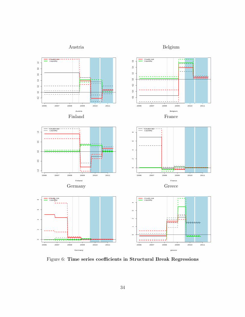
market. Our structural break analyses find that liquidity was a bigger component of bond

spread before the crisis worsens, and then the credit component starts to dominate. The

literature on delegated portfolio management has pointed out that the agency issue may

cause institutional investors to be trend chasers; buying when prices are high and selling when

prices are low in order to attract/retain fund flows. Our findings are consistent with this

interpretation: prior to the crisis of 2007 institutional bond investors are less informed about

the difference in fundamentals in the Euro area, and most price discovery was conducted in

2

the CDS market where hedge funds and other types of arbitrageurs are active players .

However, when the crisis of 2007 struck, institutional investors over-react, initially they flee

to liquidity, that is, the bond market with a lot of liquidity such as Italy and France; as the

fundamental worsens, they flee to quality such as Germany.

Our findings on liquidity to some extent are surprising but intuitive. We find via the

structural break analyses that liquidity plays a minor role in bond yield determination until

2008, after the Lehman crisis and this role is quickly reduced after late 2009. That is,

during the early stage of the Euro sovereign crisis, the market is characterized by flight to

liquidity, but the later stage, the credit risk is the main driver of bond yields and the market

is characterized by flight to quality. Further, our VAR analysis find that credit shocks are

very persistent while the liquidity shocks tend instead to die off very quickly; there is also a

feedback from country-specific credit risk to country-specific liquidity but not vice versa; and

finally there is a contagion from the Euro-area aggregate credit risk to the country-specific

credit risk, but not from aggregate liquidity to the country-specific credit risk. This set of

results indicate that the Euro sovereign bond crisis is less a liquidity crisis but a crisis induced

by common fundamentals. However, an alternative interoperation of this result is that the

heavy liquidity injection of ECB may have stopped the Euro sovereign crisis becoming a

liquidity crisis but have not stopped the contagion from the fundamental channel.

2 The Model and Testable Hypotheses

In this section, to guide the empirical analysis, we provide a stylized model to analyze

the feedback effect between the credit risk and the liquidity risk in sovereign bond market.

The model is a reduced form of the feedback model in Ozdenoren and Yuan (2008).

3

We consider a one-period economy with two types of assets, a riskless bond and many

risky assets. The riskless bond can be thought as the numeraire asset with a price of one

and the rate of return of zero. A risky asset indexed by i can be thought as the risky bond

from sovereign country i. We assume it has a supply of Mi and its payoff is as follows,

vi = βif + γPi + εi (1)

where vi denotes its final period payoff, f the Euro area aggregate fundamental credit risk, εi

sovereign-specific credit risk. The random variables f and εi are independently and normally

distributed with mean f and zero, standard deviation σf and σε respectively. The coefficient

βi sovereign country i’s loading on the Euro area aggregate risk. Finally Pi is sovereign i’s

bond price and γ measures the feedback effect from price to its fundamental value. This is

to capture the fact that lower the bond price, the hard it is for a country to come to the

bond market to raise funding for debt rollover or other fiscal budgetary needs.

There are three types of traders in this market. One is fundamental-driven traders who

trade on signals related to the fundamental worthiness of the risky assets. The signals they

receive are of two types: country-specific si and aggregate sf . They are specified as follows

sf = f + ηf , si = εi + ηi, (2)

where ηf and ηi are normally distributed with mean zero and standard deviation of σηf and

σηi respectively. We assume that these fundamental-driven traders receive identical signals

and have CARA preferences so that u(w) = −exp(−rw).

The second type of the traders are typical bond fund investors. They trade based on

4

past performance of the asset class. We model this trading behavior as follows:

L(Pi) = δPi + λσyy. (3)

That is, they increase their investment in sovereign country i’s bond when its price is high and

reduce it otherwise. Their investment has a noise component y which is normally distributed

with zero mean and standard deviation of one.

The third type of traders are noise traders and their demand is denoted as σz z which is

also normally distributed with zero mean and standard deviation of one.

With this simple setup, we solve for the optimal demand by the the fundamental-driven

traders and then solve for the equilibrium bond price through the market clearing condition.

The equilibrium price is given by,

Pi = a0 + afsf + aesi + ayλ(σyy + σz z) (4)

where

a0 =1

rβ2i

τf+τηf+ 1τε+τηi

(1− γ)− δ

1β2i

τf+τηf+ 1

τε+τηi

τf f

τf + τηfβi −M

(5)

af =1

rβ2i


(1− γ)− δ× 1

β2i

τf+τηf+ 1

τε+τηi

τηfτf + τηf

βi (6)

ae =1

rβ2i


(1− γ)− δ× 1

β2i

τf+τηf+ 1

τε+τηi

τηiτf + τηi

(7)

ay =1

rβ2i


(1− γ)− δ(8)

A few comments on this price function are in order. First, prices would over-react to the

5

shocks in the aggregate fundamental credit risk, country-specific fundamental credit risk, and

liquidity risk if there is a feedback from price to the country’s fundamental, that is, when

δ or γ is non-zero. This over-reaction may show up as contagion from the aggregate credit

risk (f). Second, the over-reaction may be different with respect to the aggregate credit risk

shock, country-specific credit risk shock, and liquidity risk depending on the perceived risk

of the fundamentals (i.e., precision of the signals) and the magnitude of the liquidity risk.

For example, when the signal about the aggregate fundamental is relatively precise, that is,

τηf is relatively large, compared with the liquidity risk (σy), prices over react more to the

liquidity shock relatively. In the empirical part of the paper, we test for the structural breaks

in the coefficients on f , ε and y to gauge how changes in the information environment affects

the bond prices.

We can substitute the above price function to (1) to decompose various shocks to country

i’ fundamentals.

vi = γa0 + (βi + γaf ) f︸︷︷︸Aggregate Credit Risk

+ (γae + 1) εi︸︷︷︸Country-Specific Credit Risk

+ γ (af ηf + aeηi)︸︷︷︸Noisy Information

+ γ(σyy + σz z)︸︷︷︸Liquidity Risk

(9)

This equation shows that the country’s fundamental is more sensitive to the aggregate

fundamental shock than to the liquidity shock as af < 1. By substituting the above equation

to (3), we find that the institutional investors’ demand is heavily influenced by the funda-

mental shocks to L(P ). That is there is a potential spillover from the aggregate as well as

the idiosyncratic fundamentals to the liquidity. In the empirical part of the paper, we test

for the existence of such feedbacks from credit risk to liquidity and vice versa.

6

3 Methodology

3.1 Bond Yields and Structure Break

We identify break dates using country specific linear regressions in which we allow for

m break points (were the optimal m is endogenously determined as described below). That

is, we allow the regression coefficients to shift from one stable regression relationship to a

different one. Thus, there are m+1 segments in which the regression coefficients are constant,

and the econometric model can be written as

yt = x′tβj + ut, j = 1, 2, ...,m+ 1, t = 1, ..., T

where j denotes the segment index.

The foundation for estimating breaks in time series regression models was given by Bai

(1994), and was extended to multiple breaks by (Bai, 1997a, 1997b) and Bai and Perron

(1998). Our approach is similar in spirit to the algorithm of Bai and Perron (2003) for the

simultaneous estimation of multiple breakpoints. We choose the optimal number of breaks

for each country as the one that minimizes the Bayesian Information Criterion (BIC) but,

differently from the previous literature, we modify the BIC statistics to be robust to potential

non-stationarity in the data.

Given an integer m denoting the number of break points, for any vector of break dates

τi (m) (of length m), we denote the extended parameter set with θi ∈ Θ ⊂ Rm×dimβj . The

associated likelihood of the data is given by f (ZT |θi, τi (m)), where ZT denotes the history

of available data. From the Bayes Theorem we have that, under a flat prior over both the

parameter space and the space of possible models, the posterior probability of a specification

7

with τi (m) as break dates is proportional to the Bayes Factor, that is

Pr (τi (m) |ZT ) ∝∫

Θ

f (ZT |θi, τi (m)) dθi ' (2π)dθ/2∣∣∣Σθi

∣∣∣ 12 f (ZT |θi, τi (m))

where θi is the vector of MLE estimate, Σ−1θ is the the observed information matrix (i.e.

the negative Hessian evaluated at θi), dθi is the dimension of θi, and the last equality comes

from a second order approximation of the log likelihood at the MLE. Taking logs of the last

expression we have

dθ2

ln 2π + ln f(ZT |θi, τi (m)

)− ln

∣∣∣Σθi

∣∣∣− 12. (10)

For stationary time series, under mild regularity conditions, T Σθi

p−→T→∞

Ωθi for some

constant Ωθi , and 1Tf(ZT |θi, τi (m)

)p−→

T→∞fi for some constant fi. Therefore, as T →∞ the

behavior of the log Bayes factor will be dominated by

ln f(ZT |θi, τi (m)

)− dθ

2lnT .

But minus twice the last expression is exactly the Bayesian Information Criterion (BIC) of

the specification with break dates given by τi (m)

BIC (τi (m)) = −2 ln f(ZT |θi, τi (m)

)+ dθ lnT. (11)

That is, using the BIC as selection criterion for the break dates, as suggested in the previous

literature, is asymptotically equivalent to choosing the model with the highest posterior

8

probability. Nevertheless, this equivalence does not hold if the data show non-stationary

behavior. This is an issue for our empirical application since the time series under analysis

often show departure from stationary in subsamples. Moreover, departures from stationarity

do not allow us to use standard F -test based break identification approaches.

To circumvent this issue we use as BIC statistic (minus twice) the expression in Equa-

tion 10 rather than the standard one in Equation (11). We compute this statistic for any

τi (m), and (due to sample size considerations) we consider up to a maximum number of

breaks, m, equal to 8. The optimal break dates are then identified as the ones that deliver

the smallest (modified) BIC statistic.

3.2 S-VAR Identification of Credit and Liquidity Spillovers

We use a structural VAR (S-VAR) approach to identify spillover effect of liquidity and

credit shocks. That is, we ask the data wether credit shocks have a tangible effect on bonds’

liquidity and whether liquidity shocks have significant effects on the credit risk of a country.

In particular, we consider a setting with four types of shocks: i) domestic credit shocks,

εc, ii) foreign credit shocks, εcf iii) net order flows shocks i.e. rebalancing shocks εnof ,

iv) domestic liquidity shocks, εl. These shocks are assumed to jointly drive the behaviour

of four quantities i) domestic CDS rates, xc; ii) foreign CDS rates, xcf (measured as an

averaged of foreign CDS); iii) net order flow for the country, xnof ; iv) domestic bonds

9

liquidity (percentage bid-ask spread), xl. For each country, the resulting S-VAR is

Γ0

xct

xcft

xnoft

xlt

︸︷︷︸≡Xt

+ Γ (L)Xt−1 = c+

εct

εcft

εnoft

εlt

︸︷︷︸≡εt

∼ N (0, I) (12)

where Γ0 is a full rank matrix capturing the contemporaneous interactions among variables,

and Γ (L) is a square matrix of polynomials of order p in the lag operator L (i.e. Γ (L) ≡

Γ1 + Γ2L1 + ... + Γp+1L

p), c is a vector of constants, and εt contains the structural shocks

that are normalized to have unit variance (this normalization is innocuous – alternatively,

we could have normalized the diagonal elements of the Γ0 matrix).

Not imposing zero restrictions on elements of Γ0 implies that all the variables can poten-

tially respond contemporaneously to all the shocks considered – that is, we don’t make any

slow reaction assumption about the variables in the S-VAR.

The above system can be rewritten in reduced form as

Xt = γ +B (L)Xt−1 + vt ∼ N (0,Ω) (13)

where B (L) ≡ −Γ−10 Γ (L) = B0+B1L+...+BpL

p and γ = Γ−10 c. The reduced form gives in γ

and B (L) as many parameters as in c and Γ1, ...Γp. Moreover, we have that by construction

Γ−10

(Γ−1

0

)′= Ω since vt = Γ−1

0 εt. So we could hope to recover Γ0 from the covariance matrix

of vt. The problem is that there are there are (n+ 1)n/2 free elements in Γ−10

(Γ−1

0

)′while

Γ0 has n2 = 4. This means that if we want to identify the structural parameters we need at

10

least (n− 1)n/2 restrictions.

The most common way of achieving identification in S-VARs is to impose some zero

restrictions on the elements of Γ0, but this would be unappealing in our setting since it

would imply that some of the financial variables considered react with delay to some of

the shocks considered. The alternative approach that we use is based instead on imposing

restrictions on the long run effect of the different types of shocks (see e.g. Blanchard and

Quah (1989)).

A natural restriction is that transitory liquidity shocks should have no effect on the credit

spreads, nor on portfolio rebalancing, in the infinite future. The idea is that a reduction

of liquidity implies a reduction of the likelihood of matching with a counterparty willing to

take the other side in an economic transaction. This implies that, when liquidity is reduced,

to be able to complete an economic transaction a premium has to be paid to complete the

transaction without delay. Therefore, a liquidity shock can potentially have a short run

effect on the credit spread. Similarly, liquidity shocks can have a short run effect on net

order flows if they generate a flight to liquidity. Nevertheless, looking in the infinite future,

the probability of matching a counterparty is one (unless there is a market shut down i.e. a

permanent liquidity shock), therefore transitory liquidity shocks should not have any effects

on the credit spread in the infinite future. Similarly, transitory liquidity shocks should not

affect net order flows in the infinite future. This long run neutrality assumption allows us

to identify the liquidity shocks. To be able to identify the other shocks we make two further

assumptions: i) transitory net order flows shocks should have no long run effects on CDS

rates since, in the long run, the latter should be pinned down only by economic fundamentals;

ii) foreign CDS shocks should not have a long run effect on domestic CDS since the former,

in the long run, should be pinned down by the country specific fundamentals that determine

11

the likelihood of default.

Rewriting the S-VAR in it’s moving average form we have

xct

xcft

xnoft

xlt

︸︷︷︸≡Xt

= k + A (L)

εct

εcft

εnoft

εlt

︸︷︷︸≡εt

∼ N (0, I) (14)

where A (L) ≡ [Γ0 + LΓ (L)]−1 = A0 + A1L + A2L2 + ...A∞L

∞. The long run restrictions

outlined above can be simply written as

∞∑j=0

Aj1,2 =∞∑j=0

Aj1,3 =∞∑j=0

Aj1,4 =∞∑j=0

Aj2,3 =∞∑j=0

Aj2,4 =∞∑j=0

Aj3,4 = 0 (15)

where the .i,l operator returns the (i, l) element of the matrix. The above restrictions

imply that A (1) ≡ A0 + A1 + A2 + ... should be a lower triangular matrix, therefore this

gives us exactly the (n− 1)n/2 restrictions needed to recover the S-VAR coefficients from

the reduced form VAR in equation (13).

Note also that under these restrictions, conditional on knowing B (L) and Ω, Γ0 and

Γ (L) are deterministic matrices. This implies that, under a diffuse prior, we can construct

posterior confidence intervals for Γ0, and for the resulting impulse-response functions, by

taking draws from the Normal-inverse-Wishart posterior of the reduce form VAR – that is,

we can construct Bayesian confidence intervals that are robust to close to unit root behavior

of the variables in the samples considered. Similarly, to avoid issues with close to unit root

behavior, the optimal number of lags is chosen using the modified BIC in Equation 10.

12

Note that, due to data limitations, we do not allow for structural breaks in the S-VAR

specification. Nevertheless, as pointed out in Sims (1987) and Leeper and Zha (2003) VARs

are best thought of as a linear approximations to the behavior of the private sector, and the

behavior they model implicitly includes dynamics arising from revisions in the forecasting

rules (as well as other sources of dynamics). As a consequence, a SVAR is likely to do

a good job in projecting the impact of credit and liquidity shocks as long as the model’s

nonlinearities generated by regime shifts are not too severe.

4 Data and Variable Construction

We use three main sources of data. First, the European government bond transaction

data is from the MTS (Mercato dei Titoli de Stato) system. Second, the credit default

swap spread data is from the Markit. Inc. Third, the Euro-denominated interest rate swaps

and the bid/ask CDS price is from Bloomberg. The sample period for our study is from

January 2, 2006 to May 31, 2011 in a daily frequency. This time period provides a good

platform to study the behavior of European government bonds markets before/during/after

the European sovereign debt crisis. Specifically, this time period includes a number of

significant credit events that directly affect the credit risk and liquidity risk in the government

bond yields, for example, the Lehman Brothers bankruptcy, the banking crisis in Ireland,

and a series of downgrading events on Greece, Ireland, Italy, Portugal and Spain.

4.1 European Bond Market

The MTS system is the largest interdealer market for Euro-denominated government

bonds. MTS Time Series data is based on the MTS interdealer markets including Eu-

13

roMTS, EuroCredit MTS and the various domestic MTS markets. The database as of May

2011 includes government bond trade data for twelve countries: Austria, Belgium, Finland,

France, Germany, Greece, Ireland, Italy, Netherlands, Portugal, Slovenia and Spain. We

exclude Slovenia from our sample for the sparsity of the data.

The MTS data contains both bond reference information (issuer, coupon rate, coupon

frequency, maturity) and detailed transaction information including trading market indica-

tor, trading price and size, order flow, and average bid/ask spread in the daily frequency.

The key variable in our study is the government bond yield which is based on the midprice,

a flat price quote based on the average of the best bid/offer prices at or before 5pm Central

European Time. To be qualified in our sample, all bonds need to meet the following criteria:

1) issued by a government (excluding quasi-government securities or structured securities);

2) traded in Euros; 3) having valid records on midprice and bid/ask spread. To minimize

the impact of confounding effects related to special bond features, we exclude securities with

floating rate coupons, inflation- or index-linked securities. To check the heterogeneity across

maturities, we split the bonds into four categories based on their remaining time-to-maturity:

2-4 years, 4-6 years, 6-8 years, 9-11 years. The rationale for these four maturity categories

is that we can match the bond data with corresponding sovereign CDS data (3-, 5-, 7-, and

10-year).

The MTS data is compiled from two different interdealer markets, the EuroMTS and

the various domestic MTS markets. According to Dufour and Skinner (2010) and the MTS

data manual, “EuroMTS is the reference electronic market for Euro benchmark bonds, or

bonds with an outstanding value of at least e 5 billion.” The MTS domestic markets lists the

whole yield curve of the government securities for each country. The majority of dealers are

members of both markets, and are therefore allowed to parallel quote, namely they post their

14

quotes on both markets simultaneously. Parallel quotes will have the same prices although

may specify different sizes on the domestic and benchmark markets. Additionally, whenever

a proposal is aggressed in one market, the dealer’s position is immediately updated on both

markets. Due to the transparency of these two systems, any differences in price or liquidity

are eliminated by arbitrageurs.

Beber, Brandt, and Kavajecz (2009) also use the MTS data but for a different sample

period, April 2003 to December 2004. They report the summary statistics uniquely based on

the benchmark market given the reason that the benchmark market lists newly issued bonds

and hence are effectively on-the-run securities. However, Dufour and Skinner (2010) make no

indication that only newly issued bonds are listed in the benchmark market. In our sample,

we use the data from the benchmark as well as the domestic market. Therefore a single

bond may have multiple entries at a given day, however all entries share the same price (may

have different trading volume). Such an arrangement allows us to construct open interest

and order flow variables from both markets in order to capture complete information.

4.2 Sovereign CDS Market

Credit-Default Swap (CDS) is a financial derivative contract which functions as an in-

surance against credit events that happen to a reference entity such as a corporate company.

One special type of reference entity is the sovereign government. The reference obligation

for sovereign credit-default swap contract is designated as senior external debt or interna-

tional debt. According to the ISDA 2004 Sovereign Master Credit Derivatives Confirmation

agreement, credit events that trigger a sovereign CDS contract include failure to pay, repu-

diation/moratorium and restructuring.

To illustrate how a sovereign CDS works, consider the case of Greece. The spread for

15

a 5-year CDS contract on Hellenic Republic rose to 1420.43 basis points on May 31, 2011.

This means a trader would have to pay USD 1,420,430 a year to insure a notional USD 10

million of the Greek debt for a pre-contracted credit event. If no such credit event happens,

the protection buyer would pay this annuity for the full five-year horizon of the contract. If

a credit event happens, however, the protection buyer could sell the sovereign bond to the

protection seller at a par value (or obtain the cash equivalent of the net gain), and terminate

the contract. In addition to physical settlement, one can opt for cash settlement, where the

protection buyer does not deliver any obligations and instead the protection seller pays the

difference between par and the recovery rate.1

Sovereign CDS has several unique features. The first aspect is that the currency of the

CDS differs from the currency of the sovereign entity. The currency of euro-area sovereign

CDS is generally in U.S. dollars. This convention was chosen in order to protect the protec-

tion buyer against inflation risk and foreign exchange risk. Secondly, the reference obligation

does not have to be of the same maturity as the CDS contract because all sovereign bonds

issued by one issuer rank pari passu with each other. In sovereign CDS, the reference debt

instruments have the same seniority, while in the corporate bond world there are different

levels of seniority and subordination of obligations.

Market participants in the sovereign CDS market often are macro hedge funds which use

sovereign CDS to express directional views on sovereign debt markets particularly since the

considerable rise in LIBOR rates made funding in the cash market more expensive. Nonethe-

less, the use of sovereign CDS has grown much broader over the recent years. Credit funds,

real money managers, structured credit investors and proprietary trading desks became active

1Similar to the physical settlement case, the protection buyer retaining the underlying deliverable obliga-tion bond will be able to sell the bond at the distressed prices in the market and thereby obtain the “recoveryrate”, thus restoring total proceeds back to par. An explicit recovery rate is typically determined by a pollof market quotations for a deliverable obligation or the reference obligation.

16

in the sovereign CDS market to take directional bets on the credit risk of European coun-

tries. In particular, anecdotal evidence suggests that these investors were using sovereign

CDS also for counterparty risk management purposes, and hedging systemic ‘tail’ risk. For

example, banks have used sovereign CDS to reduce exposure to either sovereign exposure or

bank loans to corporate within a country over recent months.

We obtain the time-series CDS price from Markit.Inc for the 3-, 5- 7- and 10-year ma-

turities for each country. They are denominated in US dollars and have the cumulative

restructuring clause. We download the bid-ask spread for CDS with five-year maturity from

Bloomberg.2 We supplement the CDS pricing data with CDS transaction information from

the Depository Trust and Clearing Corporation (DTCC), including net notional outstand-

ing, the number of CDS contract, new trades. The CDS transaction data spans the period

of September 2008 (corresponding to the beginning of the DTCC data set) to May 2011 at

a weekly frequency.

4.3 Variable Construction

In this paper we study the role of flight-to-liquidity and flight-to-safety in explaining the

European government bond yield spreads. First, we construct the bond yield spreads by

subtracting the Euro-denominated interest rate swap from the bond yield with the same

maturity. As noted by Dunne, Moore, and Portes (2003) and Beber, Brandt, and Kavajecz

(2009), the Euro-swap rate serving as the benchmark is preferred by market participants

and academic researchers, since the government bonds are less than an ideal proxy for the

unobserved risk-free rate due to taxation treatment, repo specials, and scarcity premia.

2For many countries, the bid/ask price is missing for non-five year maturity. We use the bid/ask spreadfor CDS with five-year maturity as proxy of general liquidity in the sovereign CDS market.

17

Moreover, the use of interest rate swaps provides a homogeneous benchmark across the

euro-zone area (Fontana and Scheicher (2010)) and provides explicit quotes for the 3-, 5-, 7-,

10-year maturities.

We use the sovereign credit default swap spreads as the proxy of the credit risk embedded

in the government bond yield spreads. Sovereign CDS offers a direct measure of the credit

quality on sovereign government. . The CDS data is available in the daily frequency, which

can timely capture the overall credit risk perceived by the market, as opposed to an indirect

estimate by using low frequency national account variables.

4.4 Descriptive Statistics

Table 1 presents important bond characteristics in the European government bond mar-

ket. There are overall 702 bonds issued by 11 countries in our sample. Italy has the largest

bond market with 145 bonds and an average monthly trading volume of e 45.46 billions.

France is next to Italy, with 142 bonds and e 6.65 billions trading volume on average per

month. The market also observes large trading transactions for countries like Belgium,

Netherlands, Spain, and Portugal. The average remaining time-to-maturity in our bond

sample is 5.53 years. The average coupon rate is 4.22 percent, and the average transaction

price is 100.78, close to par value. In terms of bid-ask spread, Greece and Spain have the

wider spread.

Panels B to F in Table 1 also show the bond characteristics for 3-, 5-, 7-, 10-year maturity

categories. There exists a heterogeneity of bond characteristics across countries and over

various maturities. Here we summarize three interesting findings. First, the short-term

bond with on average 3-year maturity is most traded in the European bond market with a

monthly trading volume of e 2.65 billions; the next most traded bonds are those with 5-year

18

(e 1.95 billions), then with 10-year time-to-maturity (e 1.80 billions). Second, the 10-year

bond category has the widest bid-ask spread, say 0.118, whereas the 3-year bond category

has the narrowest bid-ask spread, that is 0.069. In general bonds with longer maturity tend

to have wider bid-ask spreads on average across countries. Third, the market witnesses a

selling pressure on the 5-year bond category, measured by the net order flow (buy minus sell

orders).

4.5 Preliminary Look: Price Discovery

Financial engineers suggest that a sovereign CDS contract can replicate a position in

a cash bond as the protection seller assumes the credit risk of the reference entity. In

theory, under some conditions, an arbitrage relation exists which implies that the CDS spread

should equal the credit spread on the deliverable bond.3 Empirically, in the emerging-market

countries Ammer and Cai (2011) found that sovereign CDS premia and bond spreads are

linked by a stable linear long-run equilibrium relationship. However, the two prices of credit

risk often diverge in the short-term, with the more liquid market tending to lead the other.

They argue that price leadership in the more liquid market is consistent with the sovereign

credit risk pricing being driven mostly by public information. In developed countries however,

Fontana and Scheicher (2010), Alper, Forni, and Gerard (2011) find mixing evidence of co-

movements between sovereign CDS spreads and bond credit spreads, where the CDS market

may or may not lead the bond market and some countries even do not observe a cointegration

between CDS and bond spreads.

Figure 5 plots the time-series evolution of five-year CDS spreads and five-year govern-

3Duffie (1999) discusses the specific conditions and show why the arbitrage relation might not exactlyhold in practice.

19

ment bond credit spreads for eleven countries during the period of 2006 to 2011. The first

impression is a significant divergence of CDS premia and bond spreads, which is defined

as the “basis”. Across countries the bases were small and stable till the summer of 2007,

then they widened and became volatile during the financial crisis and the sovereign debt

crisis. The basis is positive for most countries, indicating that CDS spread exceeds the bond

spread. However, Ireland, Greece, and Portugal observe some negative basis when their

solvency becomes a serious concern. Overall, we observe that both CDS and bond spreads

go widening significantly but at different pace. Yet we need formal tests to answer which

market leads the other in the pricing process.

[Figure 5 about here.]

As noted in Blanco, Brennan, and Marsh (2005), the appropriate method to investigate

the mechanics of price discovery is not clear. We follow the literature and use the following

vector error-correction model (VECM) to test whether information of credit risk is discovered

mainly in the sovereign CDS market or in the government bond market:

∆CDSt = α1 + λ1(CDSt−1 −Bondt−1) +

p∑i=1

β1i∆CDSt−i +

p∑i=1

γ1i∆Bondt−i + ε1,t

∆Bondt = α2 + λ2(CDSt−1 −Bondt−1) +

p∑i=1

β2i∆CDSt−i +

p∑i=1

γ2i∆Bondt−i + ε2,t

where λi stands for the speed of adjustment in corresponding market to the long-run rela-

tionship, Bond is the government bond yield subtracting the interest rate swap.

Before the formal test, we first apply the augmented Dickey-Fuller test to identify the

non-stationarity of the CDS spread and bond spreads for each country. As expected, the

test does not reject the null hypothesis of a unit root for all testing series in their levels,

20

but it does for all series in their first difference.4 Then we conduct cointegration analysis

on CDS spreads and bond spreads within the above VECM framework. Table 2 presents

the contribution to the price discovery by the CDS market, measured by the mid value

of Hasbrouck information share (HAS mid) as well as permanent factor (noted as GG) in

Gonzalo and Granger (1995).

[Table 2 about here.]

Overall, the sovereign CDS market leads the bond market.

5 Empirical Results

5.1 Bond Yield Spread Decomposition

6 Conclusion

In this paper, we examine how the credit risk and liquidity evolve over the Euro sovereign

bond crisis. We find that a significant spillover from aggregate credit risk to the individual

country’s credit risk and increased in the effect of credit on bond yield determination as

sovereign debt crisis deepens. This all indicates that the Euro sovereign bond crisis speeds

through the fundamental.

We dispute the notion that the Euro sovereign bond crisis is a liquidity one as we find

through structural break analyses and VAR analysis that the liquidity effect on the sovereign

bond yield is a short-lived one. However, the short-lived liquidity effect might be due to the

fact that ECB injected a large amount of liquidity in the Euro sovereign bonds. This is open

4We do not report the results for brevity but can provide them upon request.

21

to further research.

7 Appendix

7.1 Structural Breaks Identification

22

References

Alper, Emre, Lorenzo Forni, and Marc Gerard, 2011, Pricing of sovereign credit risk: Evi-

dence from advanced economies during the recent financial crisis, working paper, IMF.

Ammer, John, and Fang Cai, 2011, Sovereign cds and bond pricing dynamics in emerging

markets: does the cheapest-to-deliver option matter?, Journal of International Financial

Markets, Institutions and Money 21, 369–387.

Bai, J., 1994, Least squares estimation of a shift in linear processes, Journal of Time Series

Analysis 15, 453–472.

, 1997a, Estimating multiple breaks one at a time, Econometric Theory 13, 315–352.

, 1997b, Estimation of a change point in multiple regression models, Review of Eco-

nomics and Statistics 79, 551–563.

, and P. Perron, 1998, Estimating and testing linear models with multiple structural

changes, Econometrica 66, 47–78.

, 2003, Computation and analysis of multiple structural change models, Journal of

Applied Econometrics 18, 1–22.

Beber, Alessandro, Michael W. Brandt, and Kenneth A. Kavajecz, 2009, Flight-to-quality or

flight-to-liquidity? evidence from the euro-area bond market, Review of Financial Studies

22, 925–957.

Blanchard, Olivier Jean, and Danny Quah, 1989, The dynamic effects of aggregate demand

and supply disturbances, American Economic Review 79, 655–73.

23

Dufour, Alfonso, and Frank S. Skinner, 2010, MTS time series market and data description

for the european bond and repo database, Icma centre discussion papers in finance Henley

Business School, Reading University Version 5.0.

Dunne, Peter, Michael Moore, and Richard Portes, 2003, Defining benchmark status: An

application using euro-area bonds, working paper, NBER.

Fontana, Alessandro, and Martin Scheicher, 2010, An analysis of euro area sovereign cds and

their relation with government bonds, working paper, ECB.

Leeper, Eric M., and Tao Zha, 2003, Modest policy interventions, Journal of Monetary

Economics 50, 1673–1700.

Sims, Christopher A., 1987, A rational expectations framework for short run policy analysis,

in W. Barnett, and K. Singleton, ed.: New Approaches to Monetary Economics . pp.

293–310 (Cambridge University Press).

24

Tab

le1:

Sum

mar

ySta

tist

ics

ofE

uro

pea

nG

over

nm

ent

Bon

dM

arke

t

Thi

sta

ble

pres

ents

sum

mar

yst

atis

tics

for

Eur

o-ar

eaco

untr

ies’

bond

mar

kets

.#

Bon

dsis

the

tota

lnu

mbe

rof

gove

rnm

ent

bond

sin

each

mat

urit

yca

tego

ry.

Cou

pon(

%)

isth

eav

erag

eco

upon

rate

the

bond

sof

each

coun

try

pay

out.

Cou

pon

freq

isth

eav

erag

efr

eque

ncy

ofco

upon

paym

ents

per

year

.Pri

ceis

the

aver

age

mid

pric

eof

all

bond

sfo

rea

chco

untr

y.Bid

-A

skis

the

aver

age

spre

adof

bond

tran

sact

ion.

NO

Fis

the

mon

thly

-agg

rega

ted

net

orde

rflo

w(b

uym

inus

sell

orde

rs)

acro

ssal

lbo

nds

issu

edby

each

coun

try.

Tot

alVol

.is

the

mon

thly

-agg

rega

ted

tota

ltr

adin

gvo

lum

eof

gove

rnm

ents

bond

s.In

Pan

elA

we

also

show

the

aver

age

bond

mat

urit

yfo

rea

chco

untr

y.T

hesa

mpl

epe

riod

isfr

omJa

nuar

y2,

2006

toM

ay31

,20

11.

Pan

elA

:A

llM

atur

itie

s

Cou

ntry

#B

onds

Cou

pon(

%)

Cou

pon

freq

Pri

ceB

id-

Ask

NO

F(b

il)T

otal

Vol

.(bi

l)M

atur

ity

Aus

tria

224.

411.

0010

2.91

0.12

-0.1

11.

626.

97B

elgi

um12

14.

790.

6510

2.32

0.06

0.65

13.6

24.

07F

inla

nd22

4.64

1.00

103.

450.

07-0

.27

2.09

4.44

Fran

ce40

84.

190.

7010

4.92

0.12

0.47

15.3

04.

67G

erm

any

218

4.07

0.82

105.

220.

090.

038.

394.

37G

reec

e71

4.85

0.93

102.

840.

09-0

.08

4.36

5.60

Irel

and

394.

510.

8110

2.11

0.08

-0.0

90.

905.

55It

aly

338

4.32

1.44

102.

080.

080.

8577

.88

4.83

Net

herl

ands

180

4.20

0.82

103.

280.

072.

8512

.08

4.97

Por

tuga

l69

4.51

0.71

100.

080.

06-0

.05

7.81

4.39

Spai

n12

14.

740.

7010

2.12

0.10

-0.1

47.

274.

28T

otal

1609

4.38

0.89

103.

330.

090.

3713

.76

4.75

25

Table 2: Price Discovery between Government Bond and Sovereign CDS Markets

In this table we show the contribution to price discovery generated by the CDS market. The contributionsare measured by Hasbrouck information share (HAS mid) and Gonzalo-Granger permanent factor noted asGG, calculated from the vector error-correction model as below:

∆CDSt = α1 + λ1(CDSt−1 −Bondt−1) + β1

p∑i=1

∆CDSt−i + γ1

p∑i=1

∆Bondt−i + ε1,t

∆Bondt = α2 + λ2(CDSt−1 −Bondt−1) + β2

p∑i=1

∆CDSt−i + γ2

p∑i=1

∆Bondt−i + ε2,t

We report the results for the whole sample and four subsample periods: Period 1: Before the crisis is fromJanuary 2006 to August 2008, Period 2: Hedge fund crisis ranges from September 2008 to July 2009, Period3: Sovereign debt crisis (Phase I) is from August 2009 to May 2010, and Period 4: Sovereign debt crisis(Phase II) ranges from June 2010 to May 2011.

Country Hasbrouck Middle Gonzalo-Granger

Total 1 2 3 4 Total 1 2 3 4Austria 0.96 0.57 0.90 0.57 0.68 0.87 1.07 0.74 0.54 1.81Belgium 0.96 0.50 0.97 0.55 0.86 1.08 1.17 1.17 0.61 1.00Finland 0.94 0.86 0.97 0.51 0.82 1.09 1.03 1.09 0.75 1.18France 1.00 0.59 0.94 0.05 0.84 0.99 1.09 1.12 -0.30 0.77Germany 1.00 0.77 0.94 0.07 0.93 0.97 1.05 0.88 -0.48 0.86Greece 0.64 0.81 0.91 0.56 0.43 0.91 1.15 1.46 1.00 0.37Ireland 0.97 0.98 0.96 0.73 1.00 1.12 1.01 1.02 0.50 0.98Italy 0.83 0.86 0.89 0.80 0.56 0.91 1.10 0.84 0.18 0.55Netherlands 0.99 0.65 0.95 0.23 0.74 0.96 1.08 0.91 0.49 0.77Portugal 0.65 0.50 0.99 0.73 0.19 0.73 1.29 1.07 1.04 -1.82Spain 0.90 0.55 0.98 0.82 0.77 1.23 1.26 0.96 0.51 1.06Mean 0.89 0.70 0.94 0.51 0.71 0.99 1.12 1.02 0.62 0.68Median 0.96 0.65 0.95 0.56 0.77 0.97 1.09 1.02 0.61 0.86

26

Austria Belgium

2006 2007 2008 2009 2010 20110

1

2

3

4

5

6

(0,2]

[2,6)

[6,11)

>11

2006 2007 2008 2009 2010 20110

5

10

15

20

25

30

35

(0,2]

[2,6)

[6,11)

>11

Finland France

2006 2007 2008 2009 2010 20110

1

2

3

4

5

6

7

(0,2]

[2,6)

[6,11)

>11

2006 2007 2008 2009 2010 20110

5

10

15

20

25

30

(0,2]

[2,6)

[6,11)

>11

Germany Greece

2006 2007 2008 2009 2010 20110

5

10

15

20

25

(0,2]

[2,6)

[6,11)

>11

2006 2007 2008 2009 2010 20110

2

4

6

8

10

12

14

(0,2]

[2,6)

[6,11)

>11

Figure 1: Trading Volume (in Billion Euros) in the European Government Bond Markets.The monthly trading volume is the sum of daily trading volume for all bonds issued by eachcountry within each maturity category.

27

Ireland Italy

2006 2007 2008 2009 2010 20110

0.5

1

1.5

2

2.5

3

(0,2]

[2,6)

[6,11)

>11

2006 2007 2008 2009 2010 20110

20

40

60

80

100

120

140

160

180

(0,2]

[2,6)

[6,11)

>11

Netherlands Portugal

2006 2007 2008 2009 2010 20110

5

10

15

20

25

30

(0,2]

[2,6)

[6,11)

>11

2006 2007 2008 2009 2010 20110

5

10

15

20

25

30

(0,2]

[2,6)

[6,11)

>11

Spain

2006 2007 2008 2009 2010 20110

2

4

6

8

10

12

14

16

18

(0,2]

[2,6)

[6,11)

>11

Figure 1 (Cont’d): Trading Volume (in Billion Euros) in the European Government BondMarkets. The monthly trading volume is the sum of daily trading volume for all bondsissued by each country within each maturity category.

28

0.5

11.5

22.5

.05

.1.1

5.2

2006m1 2007m1 2008m1 2009m1 2010m1 2011m1

Bid−Ask (LHS)

Volume (RHS)

Austria

05

10

15

.05

.1.1

5.2

2006m1 2007m1 2008m1 2009m1 2010m1 2011m1

Bid−Ask (LHS)

Volume (RHS)

Belgium

02

46

0.0

5.1

.15

.2

2006m1 2007m1 2008m1 2009m1 2010m1 2011m1

Bid−Ask (LHS)

Volume (RHS)

Finland

05

10

15

0.1

.2.3

.4

2006m1 2007m1 2008m1 2009m1 2010m1 2011m1

Bid−Ask (LHS)

Volume (RHS)

France

24

68

10

.04

.06

.08

.1.1

2

2006m1 2007m1 2008m1 2009m1 2010m1 2011m1

Bid−Ask (LHS)

Volume (RHS)

Germany

02

46

8

02

46

810

2006m1 2007m1 2008m1 2009m1 2010m1 2011m1

Bid−Ask (LHS)

Volume (RHS)

Greece0

.51

1.5

2

0.0

5.1

.15

.2

2006m1 2007m1 2008m1 2009m1 2010m1 2011m1

Bid−Ask (LHS)

Volume (RHS)

Ireland

20

40

60

80

100

120

0.1

.2.3

2006m1 2007m1 2008m1 2009m1 2010m1 2011m1

Bid−Ask (LHS)

Volume (RHS)

Italy

05

10

15

0.0

5.1

.15

2006m1 2007m1 2008m1 2009m1 2010m1 2011m1

Bid−Ask (LHS)

Volume (RHS)

Netherlands

05

10

15

20

0.0

5.1

.15

.2

2006m1 2007m1 2008m1 2009m1 2010m1 2011m1

Bid−Ask (LHS)

Volume (RHS)

Portugal

05

10

15

01

23

4

2006m1 2007m1 2008m1 2009m1 2010m1 2011m1

Bid−Ask (LHS)

Volume (RHS)

Spain

Figure 2: Liquidity in the Government Bond Market. Volume is the percentage ofmonthly average trading volume to total outstanding volume of all bonds issued by eachcountry. Bid-Ask is the average bid-ask spread of all bonds. The sample period is fromJanuary 2006 to September 2011.

29

0.5

11.5

2

24

68

10

2006m1 2008m1 2010m1 2012m1

Bond (LHS)

CDS (RHS)

Austria

0.5

1

12

34

5

2006m1 2008m1 2010m1 2012m1

Bond (LHS)

CDS (RHS)

Belgium

0.2

.4.6

.8

02

46

810

2006m1 2008m1 2010m1 2012m1

Bond (LHS)

CDS (RHS)

Finland

0.2

.4.6

.81

−5

05

10

15

2006m1 2008m1 2010m1 2012m1

Bond (LHS)

CDS (RHS)

France

0.5

11.5

2

−5

05

10

15

2006m1 2008m1 2010m1 2012m1

Bond (LHS)

CDS (RHS)

Germany

0.1

.2.3

.4.5

−2

02

46

2006m1 2008m1 2010m1 2012m1

Bond (LHS)

CDS (RHS)

Greece0

.1.2

.3.4

.5

02

46

2006m1 2008m1 2010m1 2012m1

Bond (LHS)

CDS (RHS)

Ireland

0.1

.2.3

.4

−10

010

20

30

2006m1 2008m1 2010m1 2012m1

Bond (LHS)

CDS (RHS)

Italy

.05

.1.1

5.2

.25

.3

02

46

8

2006m1 2008m1 2010m1 2012m1

Bond (LHS)

CDS (RHS)

Netherlands

0.2

.4.6

01

23

45

2006m1 2008m1 2010m1 2012m1

Bond (LHS)

CDS (RHS)

Portugal

0.2

.4.6

.8

02

46

8

2006m1 2008m1 2010m1 2012m1

Bond (LHS)

CDS (RHS)

Spain

Figure 3: Liquidity in the Government Bond and CDS Markets. Liquidity in eachmarket is measured by the percentage bid-ask spread, which is the average bid-ask spreaddivided by mid-price. Both bond and CDS have a maturity of five years. For a smoothillustration, we present the monthly average of liquidity from daily observations. The sampleperiod is from January 2006 to September 2011.

30

Austria Belgium Finland

2006 2007 2008 2009 2010 2011−5

−4

−3

−2

−1

0

1

2x 10

−3

2006 2007 2008 2009 2010 2011−6

−4

−2

0

2

4

6

8

10

12

14x 10

−3

2006 2007 2008 2009 2010 2011−0.025

−0.02

−0.015

−0.01

−0.005

0

0.005

France Germany Greece

2006 2007 2008 2009 2010 2011−1.5

−1

−0.5

0

0.5

1

1.5

2x 10

−3

2006 2007 2008 2009 2010 2011−1.5

−1

−0.5

0

0.5

1

1.5x 10

−3

2006 2007 2008 2009 2010 2011−6

−4

−2

0

2

4

6x 10

−3

Ireland Italy Netherlands

2006 2007 2008 2009 2010 2011−10

−8

−6

−4

−2

0

2

4x 10

−3

2006 2007 2008 2009 2010 2011−6

−4

−2

0

2

4

6

8x 10

−3

2006 2007 2008 2009 2010 20110

0.01

0.02

0.03

0.04

0.05

0.06

0.07

0.08

Portugal Spain

2006 2007 2008 2009 2010 2011−0.025

−0.02

−0.015

−0.01

−0.005

0

0.005

0.01

0.015

2006 2007 2008 2009 2010 2011−5

−4

−3

−2

−1

0

1

2x 10

−3

Figure 4: Net order Flow (NOF) Ratio in the Government Bond Market. NOFRatio is the the percentage of imbalance of trade (buy minus sell orders) to the total bondoutstanding issued by each country. A negative ratio indicates net selling pressure over thesample period. The sample period is from January 2006 to September 2011.

31

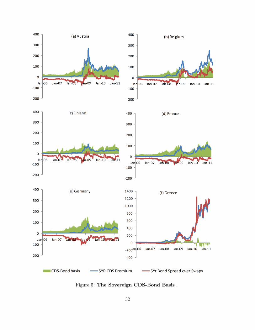
Figure 5: The Sovereign CDS-Bond Basis .

32

Figure 5 (Cont’d): The Sovereign CDS-Bond Basis.

33

Austria Belgium

2006 2007 2008 2009 2010 2011

−0.2

0.00.2

0.40.6

0.81.0

Austria

Credit riskLiquidity

2006 2007 2008 2009 2010 2011

−0.6

−0.4

−0.2

0.00.2

0.40.6

Belgium


Finland France

2006 2007 2008 2009 2010 2011

−1.0

−0.5

0.00.5

1.0

Finland


2006 2007 2008 2009 2010 2011

02

46

8

France


Germany Greece

2006 2007 2008 2009 2010 2011

02

46

8

Germany


2006 2007 2008 2009 2010 2011

01

23

4

greece


Figure 6: Time series coefficients in Structural Break Regressions

34

Ireland Italy

2006 2007 2008 2009 2010 2011

−0.2

0.00.2

0.40.6

0.81.0

Ireland


2006 2007 2008 2009 2010 2011

−1.0

−0.5

0.0

Italy



2006 2007 2008 2009 2010 2011

−1.0

−0.5

0.00.5

1.01.5

2.0

Netherlands


2006 2007 2008 2009 2010 2011

−2.5

−2.0

−1.5

−1.0

−0.5

0.00.5

Portugal


Spain

2006 2007 2008 2009 2010 2011

−10

12

34

Spain


Figure 6 (Cont’d): Time series coefficients in Structural Break Regressions

35

Austria Belgium

2006 2007 2008 2009 2010 2011

−1.0

−0.5

0.00.5

1.0

Austria

seriesfitted, no breaksfitted with breaks99% c.i.

2006 2007 2008 2009 2010 2011

−1.5

−1.0

−0.5

0.00.5

1.0

Belgium


Finland France

2006 2007 2008 2009 2010 2011

−0.5

0.00.5

1.0

Finland


2006 2007 2008 2009 2010 2011

−1.0

−0.5

0.00.5

France


Germany Greece

2006 2007 2008 2009 2010 2011

−1.2

−1.0

−0.8

−0.6

−0.4

−0.2

Germany


2006 2007 2008 2009 2010 2011

02

46

8

greece


Figure 7: Structural Break Points Identification

36

Ireland Italy

2006 2007 2008 2009 2010 2011

01

23

Ireland


2006 2007 2008 2009 2010 2011

−0.5

0.00.5

1.0

Italy



2006 2007 2008 2009 2010 2011

−0.6

−0.4

−0.2

0.00.2

0.40.6

Netherlands


2006 2007 2008 2009 2010 2011

01

23

4

Portugal


Spain

2006 2007 2008 2009 2010 2011

−0.5

0.00.5

1.01.5

2.02.5

3.0

Spain


Figure 7 (Cont’d): Structural Break Points Identification

37

a forensic analysis of liquidity and credit risk in ... · pdf filea forensic analysis of...

Documents