A Finite Element Based Formulation for Sensitivity

Studies of Piezoelectric Systems

M. A. Perry, R. A. Bates, M. A. Atherton ∗, H. P. Wynn

Dept of Statistics, London School of Economics, London WC2A 2AE, UK* School of Engineering and Design, Brunel University, UK

E-mail: m.perry@lse.ac.uk

Abstract. Sensitivity Analysis is a branch of numerical analysis which aims toquantify the affects that variability in the parameters of a numerical model have on themodel output. A finite element based sensitivity analysis formulation for piezoelectricmedia is developed here and implemented to simulate the operational and sensitivitycharacteristics of a piezoelectric based distributed mode actuator (DMA). The workacts as a starting point for robustness analysis in the DMA technology.

2

1. Introduction

Finite element methods and formulations for dynamic modelling of piezoelectric media

have been the focus of many studies [1] [2] since the original work of Allik and Hughes

[3].

Local sensitivity analysis is a branch of numerical modeling which aims to quantify the

affects of variation in individual parameters on the solution variables of differential

equation models by means of partial derivatives [4] [5] and has found widespread

scientific applications [6] [7]. Finite element methods for performing sensitivity analysis

methods are well established [8] [9] [10] [11] [12]. A common approach is to conduct

sensitivity analysis on the discretised finite element model by differentiating the standard

stiffness matrices with respect to a parameter. The adjoint sensitivity method is

beneficial in cases where the number of parameters greatly exceeds the number of

outputs. For example Kapadia et al [13] apply the adjoint method to a fuel cell

system with 180,000 design variables. This is several orders of magnitude greater

than the number of piezoelectric parameters considered in this paper and therefore the

computational advantage of the adjoint method has to be weighed against it complexity

of its implementation.

In the work presented here a finite element local sensitivity analysis formulation is

applied to the governing equations of piezoelectric media and implemented to simulate

the relative importance of design parameter variability in a piezoelectric based cantilever

beam actuator application. The analysis is performed by directly differentiating the

semi-discretised (time continuous-spatially discrete) governing equations of motion and

integrating the resulting equations using a time stepping algorithm, following the

methodology outlined in [8].

2. Governing Equations of Piezoelectric Theory

The dynamic electro-elastic response of a piezoelectric body of volume Ω and regular

boundary surface S is governed by a coupled system of electrostatic and mechanical

equilibrium boundary value partial differential equations.

The electrostatic boundary value system is defined by

∂Di

∂xi

= qv in Ω (1)

subject to the boundary condition

Dini = −qs on S (2)

and the mechanical boundary value system is defined by

∂σji

∂xj

= ρ∂2ui

∂t2in Ω (3)

subject to

σjinj = ti on S (4)

3

where qs, qv and ρ are surface charge, volume charge, and mass density respectively,

xi are spatial cartesian vector components, ni are components of the outward normal

of S and ti are components of a traction vector applied to S. Following usual tensor

convention, repeated subscripts indicate summation. σij and Di are components of the

symmetric Cauchy stress tensor (σji = σij) and electrical flux vector respectively, and

are related to those of the strain tensor εij and electric field vector Ei through the

piezoelectric constitutive equations

σij = Cijklεkl − ekijEk (5)

Di = eiklεkl + κijEj (6)

where Cijkl, ekij, and κik denote elastic, piezoelectric and dielectric material constants

respectively. The strain and electrical field components are linked to mechanical

displacement components ui and electric field scalar potential φ by

εij =1

2

(∂ui

∂xj

+∂uj

∂xi

)(7)

Ei = − ∂φ

∂xi

(8)

For arbitrary virtual displacements δui and potential δφ the differential equations (1)

and (3) can be written together the weak form variational principle representation for

PZT media

−∫

Ω

ρd2ui

dt2δui∂Ω+

∫S

tiδui∂S−∫

Ω

σjiδεij∂Ω =

∫Ω

qvδφ∂Ω+

∫S

qsδφ∂S−∫

Ω

DiδEi∂Ω(9)

the details of whose derivation are outlined in [1]. Using the Rayleigh-Ritz method [14],

(9) can be discretised to give a piezoelectric finite element formulation.

3. Piezoelectric Finite Element Formulation

For 1st order 3-d tetrahedral elements each of volume Ωe with corresponding linear shape

functions N ei i = 1, ..., 4 , the displacement vector u is approximated elementally by

ue = [Nu]un (10)

where [Nu] is a matrix of elemental shape functions

[Nu] =

N e1 N e

2 N e3 N e

4 0 0 0 0 0 0 0 0

0 0 0 0 N e1 N e

2 N e3 N e

4 0 0 0 0

0 0 0 0 0 0 0 0 N e1 N e

2 N e3 N e

4

(11)

and un is the vector of elemental nodal displacement components

un = [uex1

, uex2

, uex3

, uex4

, uey1

, uey2

, uey3

, uey4

, uez1

, uez2

, uez3

, uez4

]T (12)

where for clarity the mechanical displacement components ui described are now termed

ux uy and uz, and uexi

corresponds to the value of ux at the ith node of element e .

The elemental scalar potential is similarly approximated across each element as

φe = [Nφ]φn (13)

4

where

[Nφ] = [N e1N

e2N

e3N

e4 ] (14)

and φn is the vector of elemental nodal potentials

φn = [φe1, φ

e2, φ

e3, φ

e4]

T (15)

The mechanical strain tensor (7) and the electric field vector (8) then respectively take

the discretised forms

εe = [Bu]un and Ee = −[Bφ]φn (16)

where

[Bu] =

∂∂x

0 0

0 ∂∂y

0

0 0 ∂∂z

0 ∂∂z

∂∂y

∂∂z

0 ∂∂x

∂∂y

∂∂x

0

[Nu] and [Bφ] =

[∂

∂x,

∂

∂y,

∂

∂z

]T

[Nφ] (17)

The discretised constitutive equations of piezoelectricity (5) and (6) are then

σe = [C]εe − [e]Ee (18)

De = [e]Tεe+ [κ]Ee (19)

where [C], [e] and [κ] are now matrices of elastic, piezoelectric and dielectric material

parameters respectively.

The discretised elemental form of the variational principle (9) is then given by

−∫

Ωe

δueT ρue∂Ωe +

∫Se

δueTt∂Se −∫

Ωe

[δεeT [C]εe − δεeT [e]Ee

]∂Ωe =∫

Ωe

qvδφe∂Ωe +

∫Se

qsδφe∂Se −

∫Ωe

[δEeT [e]Tεe+ δEeT [κ]Ee

]∂Ωe (20)

where u represents a double time derivative and t is a vector of the traction

components ti. (20) can be expanded to give

−δunT

∫Ωe

[Nu]T ρ[Nu]un∂Ωe + δunT

∫Se

[Nu]Tt∂Se

−δunT

∫Ωe

[Bu]T [C][Bu]un∂Ωe − δunT

∫Ωe

[Bu]T [e][Bφ]φn∂Ωe =

δφnT

∫Ωe

[Nφ]T qv∂Ωe + δφnT

∫Se

[Nφ]T qs∂Se

+δφnT

∫Ωe

[Bφ]T [e]T [Bu]un∂Ωe − δφnT

∫Ωe

[Bφ]T [κ][Bφ]φn∂Ωe (21)

Imposing the stationary requirement of the variational principle on (21), that the

integral terms corresponding to δφn and δunmust vanish, results in two independent

5

equations that define system equilibrium:∫Ωe

ρ[Nu]T [Nu]un∂Ωe −∫

Se

[Nu]Tt∂Se +∫Ωe

[Bu]T [C][Bu]un∂Ωe +

∫Ωe

[Bu]T [e][Bφ]φn∂Ωe = 0 (22)∫Ωe

[Nφ]T qv∂Ωe +

∫Se

[Nφ]T qs∂Se +∫Ωe

[Bφ]T [e]T [Bu]un∂Ωe −∫

Ωe

[Bφ]T [κ][Bφ]φn∂Ωe = 0 (23)

Equations (22) and (23) yield the elemental system of equilibrium finite element

equations

[m]un+ [Kuu]un+ [Kuφ]φn = f (24)

[Kφu]un+ [Kφφ]φn = g (25)

where the stiffness matrices are given by

[m] =

∫Ωe

ρ[Nu]T [Nu]∂Ωe

[Kuu] =

∫Ωe

[Bu]T [C][Bu]∂Ωe

[Kuφ] =

∫Ωe

[Bu]T [e]T [Bφ]∂Ωe

[Kφu] =

∫Ωe

[Bφ]T [e][Bu]∂Ωe = [Kuφ]T

[Kφφ] = −∫

Ωe

[Bφ]T [κ][Bφ]∂Ωe

and the excitation vectors by

f =

∫Se

[Nu]Tt∂Se (26)

g = −∫

Ωe

[Nφ]T qv∂Ωe −∫

Se

[Nφ]T qs∂Se (27)

The elemental system is summed over all elements to assemble a final global system.

The parametric matrices [C], [e], and [κ] in the formulation are given in full by

[C] =

c11 c12 c13 0 0 0

c21 c22 c23 0 0 0

c31 c32 c33 0 0 0

0 0 0 c44 0 0

0 0 0 0 c55 0

0 0 0 0 0 c66

(28)

[e] =

0 0 0 0 e15 0

0 0 0 e24 0 0

e31 e32 e33 0 0 0

(29)

6

[κ] =

κ11 0 0

0 κ22 0

0 0 κ33

(30)

If the piezoelectric body in question is loaded by an electric potential in the form

φ = φ0 cos wt (31)

the displacement response will adopt the form

u = u0 cos wt (32)

where ω represents the system operational frequency. With

u = −ω2u (33)

the governing system (24) and (25) is written in the single stiffness matrix from[Kuu − ω2m Kuφ

Kφu Kφφ

] un

φn

=

f

g

(34)

For a static (constant input) analysis with ω = 0 then[Kuu Kuφ

Kφu Kφφ

] un

φn

=

f

g

(35)

When analysing a piezoelectric system in n-dimensions, with N finite element nodes, the

global stiffness matrix of (34) will be symmetric and square with dimensions (n + 1)N ,

since at each of the N nodes there are n nodal displacement components and 1 nodal

scalar potential value.

4. Finite Element Sensitivity Analysis Formulation

The matrices (28)-(30) contain the piezoelectric material system parameters. A system

sensitivity analysis formulation based on the governing finite element equations is

developed here whose solution will identify the system parameters whose value changes

will have most affect on system operation by way of partial derivatives (sensitivity

coefficients).

The equations to describe the nodal system sensitivity coefficients can be derived by

directly differentiating the governing system finite element formulation with respect to

a chosen parameter.

The finite element sensitivity formulation for the elastic parameters in the matrix [C]

are defined directly from (34) by[Kuu − ω2m Kuφ

Kφu Kφφ

] ∂un

∂cij∂φn

∂cij

=

[−Kuu

c 0

0 0

] un

φn

(36)

where cij is the chosen element of the matrix [C], ∂un

∂cijand ∂φn

∂cijare vectors of the nodal

sensitivity coefficient values and

[Kuuc ] =

∫Ωe

[Bu]T∂[C]

∂cij

[Bu]∂Ωe (37)

7

Similarly, the nodal sensitivity coefficient vector corresponding to any piezoelectric

parameter eij in the matrix [e] is defined by[Kuu − ω2m Kuφ

Kφu Kφφ

] ∂un

∂eij∂φn

∂eij

=

[0 −Kuφ

e

−Kφue 0

] un

φn

(38)

where

[Kuφe ] =

∫Ωe

[Bu]T∂[e]

∂eij

[Bφ]∂Ωe = [Kφue ]T (39)

The dielectric nodal sensitivity coefficients are given by[Kuu − ω2m Kuφ

Kφu Kφφ

] ∂un

∂κij∂φn

∂κij

=

[0 0

0 Kφφκ

] un

φn

(40)

where

[Kφφκ ] =

∫Ωe

[Bφ]T∂[κ]

∂κij

[Bφ]∂Ωe (41)

and κij is any element of the dielectric matrix [κ].

The mass density ρ is a further system parameter whose nodal sensitivity coefficient

vector is given by[Kuu − ω2m Kuφ

Kφu Kφφ

] ∂un

∂ρ∂φn

∂ρ

=

[ω2mρ 0

0 0

] un

φn

(42)

where

[mρ] =

∫Ωe

[Nu]T [Nu]∂Ωe (43)

Altogether the matrix systems (36) (38) (40) and (42) are the piezoelectric elemental

finite element formulation for the nodal sensitivities of displacement and potential to

each of the parameters in the elastic, piezoelectric and dielectric matrices and the system

mass density. The sensitivity equations can be solved in parallel with the governing

system with the nodal solution vectors determined from the governing solution used to

construct the sensitivity formulation at each solution iteration.

4.1. Implementation Example

By way of example, for the case of sensitivity with respect to the parameter e31, the

elemental nodal sensitivity coefficient vector in (38) is given by∂un

∂e31∂φn

∂e31

=

[∂ue

x1

∂e31

, ...,∂ue

x4

∂e31

,∂ue

y1

∂e31

, ...,∂ue

y4

∂e31

,∂ue

z1

∂e31

, ...,∂ue

z4

∂e31

,∂φe

1

∂e31

, ...,∂φe

4

∂e31

]T

(44)

with the right hand side vector in (38), returned as the nodal solution vector to the

governing system, given byun

φn

= [ue

x1, ..., ue

x4, ue

y1, ..., ue

y4, ue

z1, ..., ue

z4, φe

1, ..., φe4]

T (45)

8

The stiffness matrix in (38) has already been determined and decomposed in the

governing solution and the matrix in (39) is determined numerically or otherwise where

∂[e]

∂e31

=

0 0 0 0 0 0

0 0 0 0 0 0

1 0 0 0 0 0

(46)

Upon constructing and solving the system (38) the sensitivity coefficients are

approximated across each element in terms of their nodal values using∂ue

∂e31∂φe

∂e31

=

[Nu 0

0 Nφ

] ∂un

∂e31∂φn

∂e31

(47)

where ∂ue

∂e31= ∂ue

∂e31(x, y, z), ∂φe

∂e31= ∂φe

∂e31(x, y, z) and the interpolating matrix in (47) has

dimension 4x16 in accordance with (11) and (14).

The elemental sensitivity equations outlined here can be summed over all elements

for a global piezoelectric finite element sensitivity analysis, and the analysis is readily

extendable to any system parameter other than e31 using the same formulation.

4.2. Normalized Sensitivity Coefficients

The sensitivity coefficient ∂ue

∂e31computed above represents a linear estimate of the

percentage change in ue as a result of a unit change in e31. With many different physical

units involved between system outputs and parameters, a more widespread measure of

sensitivity is a normalized sensitivity coefficient defined as

∂ue

∂e31

=e31

ue

∂ue

∂e31

(48)

The normalized sensitivity coefficient indicated by the overline represents a linear

estimate of the percentage change in the variable ue given a 1% change in e31. Being

independent of the original system units in this way, normalized system sensitivity

coefficients are readily comparable with each other and therefore offer a more informative

description of parameter importance [7].

By defining new system sensitivity stiffness matrix terms as

[Kuu − ω2m]ij =1

e31

[Kuu − ω2m]ijunj i = 1, ..., 12, j = 1, ..., 12.

[Kuφ]ij =1

e31

[Kuφ]ijφnj i = 1, ..., 12, j = 1, ..., 4

[Kφu]ij =1

e31

[Kφu]ijunj i = 1, ..., 4, j = 1, ..., 12

[Kφφ]ij =1

e31

[Kφφ]ijφnj i = 1, ..., 4, j = 1, ..., 4

where subscript i, j denotes the (i, j)th element of the sub matrices in (38) and subscript

j denoting the jth element of the vectors (12) and (15), then from (38) an elemental

formulation for the normalized nodal sensitivity coefficients is given by[Kuu − ω2m Kuφ

Kφu Kφφ

] ∂un

∂e31

∂φn

∂e31

=

[0 −Kuφ

e

−Kφue 0

] un

φn

(49)

9

The normalized sensitivity coefficients can be interpolated across the element in terms

of their nodal values derived from (49) in the usual way by∂ue

∂e31

∂φe

∂e31

=

[Nu 0

0 Nφ

] ∂un

∂e31

∂φn

∂e31

(50)

Modifying the original sensitivity formulation stiffness matrix to return normalized

sensitivities directly in this way is a process that avoids the numerical complications

often associated with explicitly multiplying the original sensitivity solution by a factor

of e31

ue , say, at the point where ue = 0.

5. Numerical Results

Distributed Mode Actuators (DMA) are piezoelectric based devices that can be used to

excite a flat surface in order to produce sound. The DMA comprises one or more small

piezoelectric crystal layers, each separated by an electrode layer and attached to a sup-

porting beam. The overall assembly is clamped at one end to a common stub to make

a cantilever beam. DMA’s have become widespread in micro-engineering applications

[15] and their optimisation has been the focus of much recent work [16].

A finite element model for simulation of a single piezoelectric layer DMA, as shown

in figure 1, was developed in the commercial software package COMSOL Multiphysics.

The discretised DMA system geometry of tetrahedral elements used for the finite ele-

ment simulations is presented in figure 2. The accuracy of this DMA simulation model

has been validated against experimental measurements [17].

A useful feature in COMSOL is the ability to export finite element simulation mod-

els into MATLAB. This COMSOL-MATLAB link allows models to be manipulated and

solved from within the MATLAB environment, using special MATLAB functions pro-

vided by COMSOL. This feature was used to import the DMA simulation model into

MATLAB where it was modified according to the formulation presented in Section 4 and

solved to produce not only the standard system responses, but also the corresponding

sensitivity solutions. In this way, the sensitivities are computed at reduced computa-

tional cost, when compared with traditional finite difference methods, as the sensitivity

formulation presented in Section 4 is always linear.

Here we present simulation results on a DMA comprising of the lead zirconate

titanate ceramic PbZr0.53Ti0.47O3 (PZT-5H). This piezoelectric ceramic has relatively

large characteristic piezoelectric coupling parameter values allowing for maximal and

well controlled displacements; as such it is ideally suited for use in actuator applications.

10

Room temperature PZT-5H has characteristic material parameter matrices [18]

[C] =

1.26e11 7.95e10 8.41e10 0 0 0

7.95e10 1.26e11 8.41e10 0 0 0

8.41e10 8.41e10 1.17e11 0 0 0

0 0 0 2.3e10 0 0

0 0 0 0 2.3e10 0

0 0 0 0 0 2.33e10

(GPa) (51)

[e] =

0 0 0 0 17 0

0 0 0 17 0 0

−6.5 −6.5 23.3 0 0 0

(C/m2) (52)

[κ] =

1.503e−8 0 0

0 1.503e−8 0

0 0 1.3e−8

(F/m) (53)

and ρ = 7500kg/m3.

The simulated static displacement response of the single layer PZT-5H based DMA

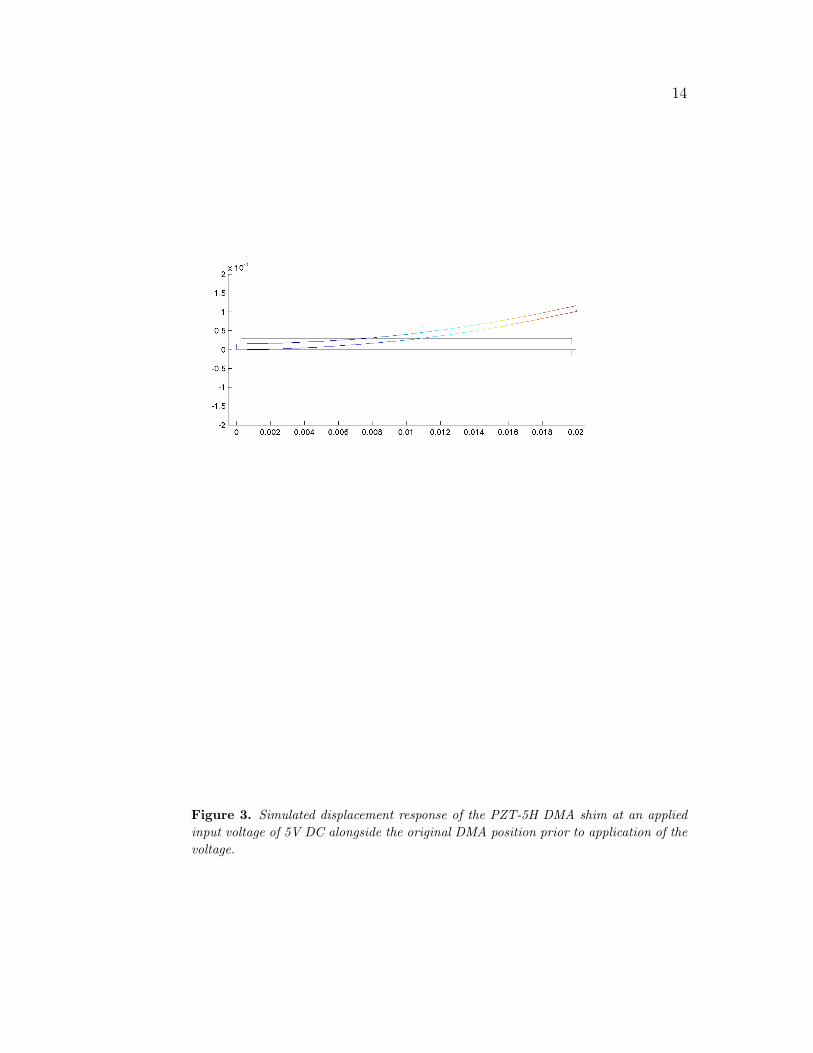
under the influence of an input DC voltage of 5V is presented in figure 3.

In the piezoelectric matrix (52), e31 = e32 and e24 = e15, such that there are three

piezoelectric material parameters to consider in a sensitivity study of a PZT-5H based

application. It is these three parameters that are subject to variation under the influence

of temperature changes [19], and as such tolerance to these potential variations is of

interest from a design perspective.

The sensitivity coefficients ∂u∂eij

for each of the piezoelectric parameters e31 e33 and e15,

simulated by solving finite element formulation in section 4, are plotted in figure 4

against distance along the DMA. The sensitivity calculations are also performed using

the finite difference method, that is by changing the relevant parameters by 1 unit and

observing the simulated change in beam displacement returned by the governing model,

are also presented in figure 4. If δ is considered to be a unit change in parameter eij,

the finite difference calculations are performed using the standard approximation

∂u

∂eij

≈ u(eij + δ)− u(eij)

δ(54)

The normalised sensitivity coefficients, simulated by solving the formulation outlined in

section 49, are presented in figure 5 alongside the corresponding finite difference results.

Normalised sensitivities represent the percentage change in output displacement given

a 1% change in the parameters. These values are seen to be uniform along the length

of the beam, indicating that beam displacement in figure 3 is proportional to the sensi-

tivity coefficient values in figure 4.

The good agreement between the analytical and empirical sensitivity results in both

figures 4 and 5 acts as a validation of the sensitivity analysis finite element formulation

for piezoelectric media. However, analytical sensitivity analysis methods hold computa-

tional advantages over empirical studies since empirical studies often require repeated

11

re-runs of a governing non-linear system where as the sensitivity equations are always

linear [20] .

In figure 4 it can be seen that changing e31 by 1 unit has more impact on the output

displacement of the DMA than a similar change in any of the other piezoelectric pa-

rameters. However, from the normalised sensitivity results in figure 5, as a percentage

of nominal value, it is seen that changes in e33 will have most effect on system output.

This comparison is evidence to the advantages in normalising the simulated sensitivity

coefficients prior to interpretation.

From the sensitivity analysis results, changing the value of e15 for this particular

design is seen to have no effect on DMA displacement. This is a significant result since,

of all the parameters, e15 undergoes greatest variation under the effects of changing

temperature [19], indicating that this particular design is robust to variation in e15.

Local sensitivity analysis results also provide important information for ranking the

importance of parameters and for deciding effective parameter value ranges in design

optimisation studies. They may also be used directly by gradient-based numerical

optimisation algorithms.

6. Conclusions

A finite element based formulation for sensitivity analysis studies of piezoelectric media

was developed and an existing finite element piezoelectric solver was extended to

implement its solution. The solver was applied to simulate the static operational and

sensitivity characteristics of a piezoelectric based distributed mode actuator. The finite

element sensitivity solutions were verified against empirical results obtained using the

original system model.

The sensitivity analysis was performed with respect to the material piezoelectric

coupling parameters since it is these parameters that are subject to variability under

operational conditions. As such, these sensitivity results are of interest from a robust

design perspective. However, the analysis presented here is easily extended to other

system parameters using the same basic formalism.

7. Acknowledgements

This work was supported by the Engineering & Physical Sciences Research Council

(EPSRC) at the London School of Economics under grant number GR/S63502/01 and

at Brunel University under grant number GR/S63496/02.

[1] A. Benjeddou. Advances in piezoelectric finite element modeling of adaptive structural elements:a survey. Computers and Structures, 76:347–363, 2000.

[2] J. Mackerle. Smart materials and structures - a finite element approach: a bibliography (1986-1997). Modelling and Simulation in Materials Science and Engineering, 6:293–334, 1998.

12

[3] H Allik and T. J. R. Hughes. Finite element method for piezoelectric vibration. InternationalJournal for Numerical Methods on Engineering, 2:151–157, 1970.

[4] A. M. Dunker. The decoupled direct method for calcuating sensitivity coefficients in chemicalkinetics. J. Chem. Phys, 81:2385–2393, 1984.

[5] Leis J. R. and Kramer M. A simultaneous solution and sensitivity analysis of systems describedby ordinary differential equations. ACM transactions on mathematical software, 14(1):45–60,1988.

[6] Saltelli A., Tarantola S., Campolongon F., and Ratto M. Sensitivity Analysis in Practice. Wiley,2004.

[7] A. Saltelli, K. Chan, and E. M. Scott. Sensitivity Analysis (Chapter 5). Wiley, 2000.[8] J. P. Conte, P. K. Vijalapura, and M. Meghella. Consistent finite-element response sensitivity

analysis. J. Eng. Mech, 129(12):1380–1393, 2003.[9] T. Haukaas and A. Der Kiureghian. Parameter sensitivity and importance measures in nonlinear

finite element reliability analysis. ASCE Journal of Engineering Mechanics, 131(10):1013–1026,2005.

[10] M. Kleiber, H. Antunez, T. D. Hein, and P. Kowalczyk. Parameter Sensitivity in non-linearmechanics: Theory and finite element computations. Wiley, New York., 1997.

[11] J. J. Tsay and J. S. Arora. Nonlinear structural design sensitivity analysis for path dependentproblems. part 1: General theory. Comput. Methods Appl. Mech. Eng., 81:183–208, 1990.

[12] J. J. Tsay, J. E. B. Cardoso, and J. S. Arora. Nonlinear structural design sensitivity analysis forpath dependent problems. part 2: Analytical examples. Comput. Methods Appl. Mech. Eng.,81:209–228, 1990.

[13] S. Kapadia, W. K. Anderson, L. Elliot, and C. Burdyshaw. Adjoint method for solid-oxide fuelcell simulations. Journal of Power Sources, 166:376–385, 2007.

[14] Jianming Jin. The Finite element Method in Electromagnetics. 2nd Edition. Wiley, 2002.[15] P Muralt. Ferroelectric thin films for micro-sensors and actuators: a review. Journal of

Micromechanics and Microengineering., 10:136–146., 2000.[16] M.I. Frecker. Recent advances in optimization of smart structures and actuators. Journal of

Intelligent Material Systems and Structures, 14(5):207–216., 2003.[17] Y. Shen, M.A. Atherton, M.A. Perry, R. A. Bates, and H. P. Wynn. Simulation of the

electromechanical coupling in multilayered piezoelectric distributed mode actuator. Submittedto: Sensors and Actuators: A. Physical, 2006.

[18] Piezo Systems Inc. Product Catalogue. Cambridge, MA., 1995.[19] D. Wang, Y Fotinich, and G. P. Carman. Influence of temperature on the electromechanical and

fatigue behaviour of piezoelectric ceramics. Journal of Applied Physics, 83(10):5342–5350, 1998.[20] Dariusz Ucinski. Optimal Measurement Methods for Distributed Parameter System Identification

(Chapter 2). CRC Press, 2005.

13

-7mm

)

1

20mm

PZT

Shim

PZT

6

?6

?

6

?

150µm

150µm

150µm

Figure 1. Geometry and dimensions of a single layer PZT based Distributed ModeActuator

Figure 2. The discretized DMA system model as used for the finite elementcalculations

14

Figure 3. Simulated displacement response of the PZT-5H DMA shim at an appliedinput voltage of 5V DC alongside the original DMA position prior to application of thevoltage.

15

0 0.005 0.01 0.015 0.02−10

−8

−6

−4

−2

0

2

4

6

8x 10−8

Distance along shim (m)

Dis

plac

emen

t Sen

sitiv

ity to

e (

m)

e31 (empirical)e33 (empirical)e15 (empirical)e31 (analytic)e33 (analytic)e15 (analytic)

Figure 4. Analytic and empirically simulated values of the sensitivity coefficients ∂u∂eij

plotted against distance along the shim of the PZT-5H DMA .

0 0.005 0.01 0.015 0.02

0

0.1

0.2

0.3

0.4

0.5

0.6

0.7

0.8

Distance along shim (m)

Per

cent

age

Dis

plac

emen

t Sen

sitiv

ity to

eij

e31 (empirical)e33 (empirical)e15 (empirical)e31 (analytic)e33 (analytic)e15 (analytic)

Figure 5. Analytic and empirically simulated values of the normalised sensitivitycoefficients ∂u

∂eijplotted against distance along the shim of the PZT-5H DMA .