A finite difference Hartree-Fock program for atoms and

diatomic molecules

Jacek Kobus

Instytut Fizyki, Uniwersytet Miko laja Kopernika, Grudziadzka 5, 87-100 Torun, Poland

Abstract

The newest version of the two-dimensional finite difference Hartree-Fockprogram for atoms and diatomic molecules is presented. This is an up-dated and extended version of the program published in this journal in 1996.It can be used to obtain reference, Hartree-Fock limit values of total en-ergies and multipole moments for a wide range of diatomic molecules andtheir ions in order to calibrate existing and develop new basis sets, calcu-late (hyper)polarizabilities (αzz, βzzz, γzzzz, Az,zz, Bzz,zz) of atoms, homo- andheteronuclear diatomic molecules and their ions via the finite field method,perform DFT-type calculations using LDA or B88 exchange functionals andLYP or VWN correlations ones or the Self-Consistent Multiplicative Con-stant method, perform one-particle calculations with (smooth) Coulomb andKrammers-Henneberger potentials and take account of finite nucleus models.The program is easy to install and compile (tarball+configure+make) andcan be used to perform calculations within double- or quadruple-precisionarithmetic.

Keywords: Schrodinger equation of one-electron atomic and diatomicsystems, restricted open-shell Hartree-Fock method, atoms, diatomicmolecules, density functional theory potentials, Gauss and Fermi nuclearcharge distributions, finite field method, prolate spheroidal coordinates,8th-order discretization, (multicolour) successive overrelaxation2000 MSC: 35Q40, 65N06, 65N22, 81V45, 81V55

NEW VERSION PROGRAM SUMMARYManuscript Title: A finite difference Hartree-Fock program for atoms and diatomic

molecules

Authors: Jacek Kobus

Preprint submitted to Computer Physics Communications June 15, 2012

Program Title: 2dhf

Journal Reference:

Catalogue identifier:

Licensing provisions: GPL

Programming language: Fortran 77, C

Computer: any 32- or 64-bit platform

Operating system: Unix/Linux

RAM: case dependent, from few MB to many GB

Number of processors used:

Supplementary material:

Keywords: restricted open-shell Hartreee-Fock method, DFT potentials, prolate

spheroidal coordinates, 8th-order discretization, (multicolour) successive overre-

laxation method,

Classification: 16.1

External routines/libraries:

Subprograms used:

Catalogue identifier of previous version: ADEB v1 0*

Journal reference of previous version: Comput. Phys. Commun. 98(1996)346*

Does the new version supersede the previous version?: yes*

Nature of problem: The program finds virtually exact solutions of the Hartree-

Fock and density functional theory type equations for atoms, diatomic molecules

and their ions. The lowest energy eigenstates of a given irreducible representation

and spin can be obtained. The program can be used to perform one-particle cal-

culations with (smooth) Coulomb and Krammers-Henneberger potentials and also

DFT-type calculations using LDA or B88 exchange functionals and LYP or VWN

correlations ones or the Self-Consistent Multiplicative Constant method.

Solution method: Single particle two-dimensional numerical functions (orbitals)

are used to construct an antisymmetric many-electron wave function of the re-

stricted open-shell Hartree-Fock model. The orbitals are obtained by solving the

Hartree-Fock equations as coupled two-dimensional second-order (elliptic) partial

differential equations (PDE). The Coulomb and exchange potentials are obtained

as solutions of the corresponding Poisson equations. The PDEs are discretized

by the 8th-order central difference stencil on a two-dimensional single grid and

the resulting large and sparse system of linear equations is solved by the (mul-

ticolour) successive overrelaxation method ((MC)SOR). The self-consistent-field

iterations are interwoven with the (MC)SOR ones and orbital energies and nor-

2

malization factors are used to monitor the convergence. The accuracy of solutions

depends mainly on the grid and the system under consideration which means that

within double precision arithmetic one can obtain orbitals and energies having up

to 12 significant figures. If more accurate results are needed the quadruple precison

floating-point arithmetic can be used.

Reasons for the new version: additional features, many modifications and cor-

rections, improved convergence rate, overhauled code and documentation*

Summary of revisions: see ChangeLog found in tgz archive*

Restrictions: The present version of the program is restricted to 60 orbitals. The

maximum grid size is determined at compilation time.

Unusual features: The program uses two C routines for allocating and deallocating

memory. Several BLAS (Basic Linear Algebra System) routines are emulated by

the program. When possible they should be replaced by their library equivalents.

Additional comments: automake and autoconf tools are required to build and com-

pile the program; checked with f77, gfortran and ifort compilers

Running time: Very case dependent – from a few CPU seconds for the H2 de-

fined on a small grid up to several weeks for the Hartree-Fock-limit calculations for

40-50 electron molecules.

1. INTRODUCTION

The modeling of the electronic structure of atoms and molecules has re-ceived a great deal of effort over the last 50 years. Nowadays a significantpart of CPU power available to scientific community is used to understandthe physical and chemical behaviour of molecular systems by employing arange and/or a mixture of ab initio, semi-empirical and molecular mechan-ics methods (see for example [1]). In mainstream computational quantumchemistry molecular orbitals are expressed as linear combinations of (atomic)basis functions which allows to treat systems of any composition and geom-etry. Since in practice basis sets are usually far from being complete the

3

calculated properties suffer from so called basis set truncation errors thatare difficult to assess and control. In order to tackle the problem a numberof different sequences or families of basis set functions have been developedto make calculations of various systems and properties feasible and credible.By and large calibration of basis sets is based on atomic data which canbe obtained by numerical, i.e. basis-set-free methods. That is why nearlyfifty years ago there were already first attempts to solve the HF problem formolecules by reducing it to one-center cases for which well established numer-ical methods had already been known [2, 3, 4, 5, 6]. This idea was revitalizedmany years later by Becke who proposed to solve the Hartree-Fock-Slaterequations for a general polyatomic molecule via several separate solutions ofthe appropriately defined atomic-like problems [7, 8, 9]. Recently Shiozakiand Hirata has extended this approach to the HF equations [10].

McCullough was the author of the first not fully algebraic, semi-numericaland successful attempt to solve the (multi-configuration) HF equations fordiatomic molecules called the partial-wave self-consistent-field method (PW-SCF) [11, 12]. In case of diatomic molecules one can choose a prolatespheroidal coordinate system whose centres coincide with the nuclei: ξ =(rA + rB)/RAB, η = (rA − rB)/RAB and the azimuth angles θ (0 ≤ θ ≤ 2π)where atoms A and B are placed along z-axis at points (0, 0,−RAB/2) and(0, 0,+RAB/2) and rA and rB are the distances of a given point from theseatomic centres. The cylindrical symmetry of the diatomic systems allows forfactoring out (and later treating analytically) the angular part and expressingmolecular orbitals and the corresponding Coulomb and exchange potentialsin the form f(ξ, η)eimθ where m is an integer. Thus for diatomic moleculesthree-dimensional HF equations can be reduced to their two-dimensionalcounterparts for the functions f(ξ, η). In the PWSCF method these equa-tions are further simplified by requiring that the function f has the formf(ξ, η) =

∑lmaxl=m Xm(ξ)Pm

l (η) where the associate Legendre functions Pml (η)

form a basis set in η variable (that was the reason why McCullough referredto this method as a semi-numerical one). As a result Xm(ξ) functions mustsatisfy second-order ordinary differential equations which are solved numeri-cally on a properly chosen grid. In early 1980s Becke developed a numericalapproach for solving density functional equations for diatomic molecules byusing polynomial spline interpolation for approximating the f function ona suitable chosen two-dimensional grid [13, 14, 15, 16]. The function valuesat the grid points were obtained by requiring the minimization of a certainfunctional equivalent to the given Fock-Slater equations. Recently Artemyev

4

et al. proposed a variant of PWSCF by expanding the f function in a finiteB-splines basis set; as a bonus one gets also virtual molecular orbitals thatcan be used to calculate correlation effects by the second-order perturbationtheory [17]. In the second half of the 1980s Heinemann, Fricke and coworkersshowed that the two-dimensional Hartree-Fock equations could be success-fully solved by the finite element method [18, 19, 20]. Later the multigridvariant of the method was also developed [21]. The finite element approachwas also used to solve a one-electron Schrodinger equation for the linear tri-atomic molecule H2+

3 [22] and Dirac and Dirac-Slater equations [23, 24, 25].Sundholm and Olsen have also developed a finite-element approch for solvingthe HF equations [26, 27, 28]. Recently Morrison et al. have been advocat-ing the theory of domain decomposition that could be used to divide thevariable domain of a diatomic molecule into separate regions in which theHF equations are solved independently by approximating the f function byhigh-order spline functions [29, 30]. Due to this decomposition fast iterativemethods can be applied to solve HF equations in the interior region (wherethe operators are self-ajoint) and explicite methods in the boundary ones.This scheme allows to use non-uniform multiple grids and thus solve the HFequations for both bound and continuous eigenstates.

Yet another approach to solving the HF equations for diatomic moleculeswas put forward in early 1980s by Laaksonen, Pyykko and Sundholm. Theyproposed to represent the f function through its values on a two-dimensionalmesh. To this end the second-order partial differential equations for orbitalsand potentials were discretized by means of the 6th-order cross-like stenciland the ensuing large and sparse systems of linear equations were solved bymeans of the iterative successive overrelaxation method (SOR) [31]. Thisapproach will be referred to as the finite difference HF (FD HF) method.Davstad has also developed a fully numerical finite-difference approach forthe solution of Hartree-Fock equations for diatomic molecules [32]. The FDand FE methods together with the wavelets method belong to the so calledreal-space mesh techniques used to solve Poisson, Poisson-Boltzmann andeigenvalue problems and the reader is refered to review articles by Beck [33]and Arias [34] for further details.

The present author got interested in the FD HF method about 20 yearsago and has been involved in its development and applications ever since[35, 36, 37]. An improved version of the FD HF method was announcedin 1996 [38, 39]. For many years the method was mainly used to assistthe process of development and calibration of sequences of universal even-

5

tempered basis sets that was initiated by Moncrieff and Wilson in the early1990s [40, 41, 42, 43, 44, 45, 46, 47, 48, 49, 50, 51]. In the course of thatwork the method proved to be a reliable source of reference values of totalenergies, multipole moments, static polarizabilities and hyperpolarizabilities(αzz, βzzz, γzzzz, Az,zz and Bzz,zz) for atoms, diatomic molecules and theirions [52, 53, 54, 55, 56]. It also provided HF-limit values for examining con-vergence patterns of properties calculated using correlation-consistent basissets within the context of complete basis set models [57, 58, 59, 60, 61] andeventually helped in the development of polarization-consistent basis sets[62, 63, 64]. The method was also employed to provide the reference values ofspectroscopic constants of several diatomic molecules in order to compare theconvergence patterns of the correlation-consistent and polarization-consistentbasis sets towards the complete basis set limit [65]. The FD HF energiesaccurate to at least 1µHartree were calculated for 27 diatomic transition-metal-containing species in order to investigate the convergence of the HFenergies upon increasing the sizes of correlation consistent basis sets andaugmented basis sets developed for the transition atoms by Balabanov andPeterson [66, 67]. The correlation-consistent basis sets were not constructedto allow for extrapolation of the HF total energies but rather to extrapolatethe correlation energies to the complete basis set limit. It was demonstratedthat correlation energies converge according to the inverse power law whilethe HF energies exhibit exponential behaviour both with respect to the totalnumber of the basis functions of a given type and with respect to the max-imum angular momentum functions included [68, 58]. That was the ratio-nale behind Jensen’s project to design hierarchies of polarization-consistentbasis sets specifically tailored to facilitate extrapolation of the HF (also den-sity functional theory) energies, dipole moments and equilibrium distancesto their corresponding complete basis set limits [62]. Recently, Zhong etal. presented a new family of basis sets, called n-tuple-ζ augmented polar-ized (n=2-6) basis sets, that converge systematically to the complete basisset limits of both the SCF energy and the correlation energy [69]. Jensenexamined the dependence of FD HF total energies on the grid size for 42diatomic species composed of the first and second row elements and reportedtheir energies to better than 1 µHartree accuracy [70]. Halkier and Corianiused the FD HF-limit value of the electric quadrupole moment of the hy-drogen fluoride to estimate the basis set truncation errors when performingthe state-of-the-art calculations to determine the full configuration interac-tion basis set limit value of this property [71]. This work is an apparent

6

demonstration that when accurate post-HF treatment is at stake then thebasis set development must guarantee that the HF values are also accurate.Similarly, Pawlowski et al. used the FD HF method to obtain the dipolepolarizability and the second hyperpolarizability of the Ne atom to estimatebasis set errors present in the calculations using the CCS, CC2, CCSD andCC3 coupled cluster models and Dunning’s correlation-consistent basis setscc-pVXZ augmented with diffuse functions [72].

A separate problem is the assessment of relativistic basis functions usedfor solving the Dirac-Fock equations. Although at present there is no rel-ativistic version of the FD HF method, it seems that the method can beused to indirectly assess the quality of the basis sets used for relativisticcalculations. Styszynski studied the influence of the relativistic core-valencecorrelation effects on total energies, bond lengths and fundamental frequen-cies for a series of hydrogen halide molecules (HF, HCl, HBr, HI and HAt).In order to assess the quality of basis sets and the dependence of spectro-scopic constants on the basis set truncation errors the results of the algebraicnon-relativistic HF calculations were compared with the corresponding FDHF ones [73, 74, 75].

It seems that the development and calibration of the basis sets for thecalculation of electron momentum densities also benefited from the FD HFmethod. It allowed to find large basis set errors in previous computations ofthese quantities by means of self-consistent-field wave functions often consid-ered to be of near-Hartree-Fock quality [76]. Calculation of stopping powersand ranges of energetic ions in matter within the semiempirical approachdeveloped by Ziegler, Biersack and Littmark require the knowledge of inter-atomic potentials [77]. Nordlund et al. [78] studied repulsive potentials forC-C, Si-Si, N-Si and H-Si systems and Pruneda and Artacho [79] extendedthe analysis to C-C, O-O, Si-Si, Ca-O and Ca-Ca systems by calculating thepotentials by means of the density functional theory and the HF methods(both algebraic and fully numerical). In order to test the quality of basis setsused to obtain the potentials for Kr-C, Xe-C, Au-C and Pb-C diatomics, es-pecially at small interatomic distances, the FD HF method was also employed[80, 81]. Numerical orbitals obtained from the methd also proved useful indeveloping a model of high-harmonic generation from diatomic molecules[82].

The FD HF approach proved useful in the density functional theory con-text to construct and test various functionals [83, 84, 85, 86, 87, 88, 89, 90].Calculations for systems with finite-size nuclei employing the Gauss or Fermi

7

nuclear charge distribution models can also be made [91]. It is worth notingthat if the method is applied to a one-electron system it can be treated asa finite difference solver of the Schrodinger equation for the three-dimensionalCoulomb and Krammers-Henneberger potentials (and the like) in the cylin-drical coordinates [92].

As mentioned above the universal sequences of even-tempered Gaussianbasis functions and polarization-consistent basis functions were developedwith the help of numerical results by means of the FD HF. This calibrationwork was a major stimulus for developing the method, improving its accuracy,stability and efficiency and thus enlarging its range of applicability. Thispaper aims at presenting the current version of the program (version 2.0)so that it can be confidently used and further developed should the needarise. The present version of the program is the first one with the versionnumer explicitely given as this should help to maintain the code. This workshould be viewed as an update to an earlier paper describing the methodand the previous version of the program [38]. The current and some in-between versions of the program are available from the project’s home pagehttp://www.leiflaaksonen.eu/num2d.html.

The paper is organized as follows. The introduction is followed by a gen-eral description of the restricted open-shell Hartree-Fock method for diatomicmolecules. In section 3 the discretization of second-order partial differentialequations is presented and the usage of the SOR method for solving largeand sparse systems of resulting linear equations is described in some detailas this is the crux of the presented approach. Especially the SCF/SOR it-eration patterns and the accuracy of the approach are discussed. The x2dhfprogram can be used as a solver of one-electron Schrodinger equation in twovariables. Section 4 presents additional one-electron potentials that can beselected. The final section 5 is devoted to the x2dhf program itself, its calltree, data structures and workings of the major routines responsible for theSCF and SOR iterations. In order to help checking, correcting and modifyingthe program the appendices contain various relevant formulae of DFT energyfunctionals and potentials, finite nucleus models, multipole moments, etc.

2. GENERAL DESCRIPTION

2.1. The restricted open-shell Hartree-Fock method

For a open-shell, M -electron, diatomic molecular system the Hartree-Fockequations are a set of M one-particle (integro-differential) equations (Fock

8

equations)[38, 39]

Faφa =M∑a=1

Eabφb, a = 1, . . . ,M (1)

where φa = φa(x, y, z, σ) are spin-orbitals forming the Slater determinant

Φ =1√M !

det |φ1(1), φ2(2), . . . , φM(M)|

being the approximation to the solution of the Schrodinger equation thatminimizes the energy functional

〈Φ| −∑a

1

2∇2a −

ZAraA− ZBraB

+∑a<b

1

rab+ZAZBR|Φ〉

It is assumed that atoms A and B having charges ZA and ZB are placedalong z-axis at points (0, 0,−R/2) and (0, 0,+R/2) and raA and raB are thedistances of a given particle from these atomic centres separated by R.

The Fock equations can be put in the form

−1

2∇2φa = −

(−ZAraA− ZBraB

+∑b

[V bC − V ab

x

]− Ea

)φa +

∑b6=a

Eabφb (2)

where

∇2V aC = −4πφ∗aφa

∇2V abx = −4πφ∗aφb (3)

are Poisson equations determining the electron-electron Coulomb and ex-change potentials via the single particle and the pair densities, respectively.The Fock equations are solved by the self consistent field (SCF) iterativeprocedure and therefore the right-hand-sides of Eq. (2) can be treated dur-ing each iteration as already known functions since they are determined bythe orbitals obtained in the previous iteration (and approximate potentialsare obtained via integration of Eq. (3)). Thus, not only the Coulomb andexchange potentials but also the orbitals can be obtained by solving Poisson-type equations.

9

Diatomic molecules can be described in prolate spheroidal coordinatesystem

ξ = (rA + rB)/R

η = (rA − rB)/R

θ azimuth angle

1 ≤ξ <∞−1 ≤η ≤ 1

0 ≤θ ≤ 2π

(4)

where rA and rB are the distances of a given point from the atomic centres.The cylindrical symmetry of the diatomic systems allows for factoring out(and later treating analytically) the angular part and expressing the orbitalsand the potentials in the form

φa

V aC

V abx

= f(ξ, η)eimθ (5)

where the parameter m is equal to 0, ±1, ±2, . . .. The energy expression forthe restricted open-shell Hartree-Fock (ROHF) method reads

E =∑a

〈φa| −1

2∇2 + Vn |φa〉 qa +

∑a,b

〈φa|V bC |φa〉Uab −

∑a,b

〈φa|V abx |φb〉Wab (6)

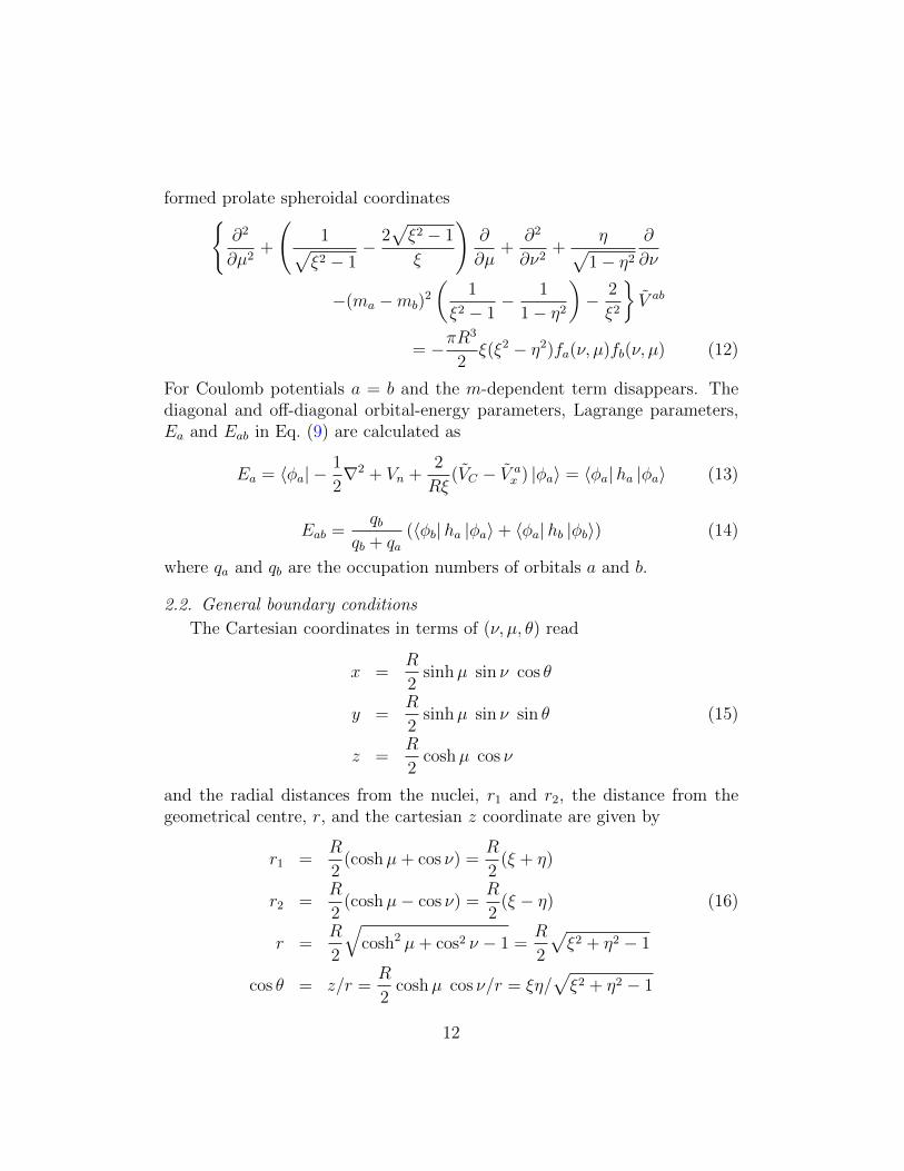
where Vn = −ZA/raA−ZB/raB is the nuclear potential energy operator. qa isthe occupation number for orbital a and Uab and Wab are the correspondingoccupation-number dependent factors for the Coulomb and exchange energycontributions. In order to allow for a more accurate description of orbitalsand potentials in the vicinity of the nuclei, the prolate spheroidal coordinates(η, ξ, θ) are transformed into the (ν, µ, θ) variables.

µ = cosh−1 ξ 0 ≤ µ ≤ ∞ν = cos−1 η 0 ≤ ν ≤ π (7)

Because of this transformation, φa is a quadratic function of µ and ν forpoints in the vicinity of the z-axis (µ = 0 corresponds to the cartesian co-ordinates (0, 0,−R/2 ≤ z ≤ R/2), ν = 0 to (0, 0, z ≥ R/2)) and ν = π to(0, 0, z ≤ −R/2). In the transformed prolate spheroidal coordinates (ν, µ, θ),the ”radial” part of the Laplacian reads

4

R2(ξ2 − η2)

{∂2

∂µ2+

ξ√ξ2 − 1

∂

∂µ+

∂2

∂ν2+

η√1− η2

∂

∂ν−m2

a

(1

ξ2 − 1+

1

1− η2

)}(8)

10

In Eq. (8), ma is an integer and defines the rotation symmetry of the orbitals.The orbitals with ma = 0 are called σ orbitals, and π orbitals have ma = ±1,δ orbitals have ma = ±2 and orbitals with ma = ±3 are called ϕ orbitalsand so on. Orbitals of higher symmetry than ϕ are not relevant for ordinarydiatomic molecules at the Hartree-Fock level. The orbitals with the same”radial” part and with m = ±ma belong to the same shell. Since the m-value for the exchange potentials, V ab, is |ma − mb|, the largest m-valuefor the exchange potentials becomes |2 ma,max|, where ma,max is the largestorbital m-value.

Multiplying the Fock equation by −R2

2(ξ2 − η2) yields the working equa-

tion for the orbital relaxation in the transformed prolate spheroidal coordi-nates. {

∂2

∂µ2+

ξ√ξ2 − 1

∂

∂µ+

∂2

∂ν2+

η√1− η2

∂

∂ν

−m2a

(1

ξ2 − 1+

1

1− η2

)+R[ξ(Z1 + Z2) + η(Z2 − Z1)]

−Rξ

(ξ2 − η2)VC +R2

2(ξ2 − η2)Ea

}fa(ν, µ)

+R

ξ(ξ2 − η2)

(Vx

a+Rξ

2

∑b 6=a

Eabfb(ν, µ)

)= 0 (9)

In Eq. (9) the modified Coulomb VC and exchange potentials V ax have been

introduced.

V aC = RξV a

C/2 V abx = RξV ab

x /2 (10)

VC =∑a

V aC V a

x =∑b6=a

V abx fb(ν, µ) (11)

The working equation for the relaxation of the Coulomb and exchangepotentials are analogously obtained from the Poisson equation in the trans-

11

formed prolate spheroidal coordinates{∂2

∂µ2+

(1√ξ2 − 1

− 2√ξ2 − 1

ξ

)∂

∂µ+

∂2

∂ν2+

η√1− η2

∂

∂ν

−(ma −mb)2

(1

ξ2 − 1− 1

1− η2

)− 2

ξ2

}V ab

= −πR3

2ξ(ξ2 − η2)fa(ν, µ)fb(ν, µ) (12)

For Coulomb potentials a = b and the m-dependent term disappears. Thediagonal and off-diagonal orbital-energy parameters, Lagrange parameters,Ea and Eab in Eq. (9) are calculated as

Ea = 〈φa| −1

2∇2 + Vn +

2

Rξ(VC − V a

x ) |φa〉 = 〈φa|ha |φa〉 (13)

Eab =qb

qb + qa(〈φb|ha |φa〉+ 〈φa|hb |φb〉) (14)

where qa and qb are the occupation numbers of orbitals a and b.

2.2. General boundary conditions

The Cartesian coordinates in terms of (ν, µ, θ) read

x =R

2sinhµ sin ν cos θ

y =R

2sinhµ sin ν sin θ (15)

z =R

2coshµ cos ν

and the radial distances from the nuclei, r1 and r2, the distance from thegeometrical centre, r, and the cartesian z coordinate are given by

r1 =R

2(coshµ+ cos ν) =

R

2(ξ + η)

r2 =R

2(coshµ− cos ν) =

R

2(ξ − η) (16)

r =R

2

√cosh2 µ+ cos2 ν − 1 =

R

2

√ξ2 + η2 − 1

cos θ = z/r =R

2coshµ cos ν/r = ξη/

√ξ2 + η2 − 1

12

Eqs. (15) reveal an interesting property of the transformation given by Eq. (7).If the sign of µ or ν is reversed then the point (x, y, z) goes over into(−x,−y, z). A rotation by π leaves orbitals with even m unchanged butreverses the sign of orbitals with odd m-values. This means that orbitalsand potentials of σ, δ, . . . symmetry are even functions of (µ, ν) and orbitalsand potentials of π, ϕ, . . . symmetry are odd ones. Thus we can write

f(ν, µ) = (−1)mf(ν,−µ)

f(ν, µ) = (−1)mf(−ν, µ) (17)

f(π + ν, µ) = (−1)mf(π − ν, µ)

These symmetry relations can be readily used to set the values of f to zeroalong (ν, 0), (0, µ) and (π, µ) boundary lines for orbitals of π, ϕ, . . . symmetry.In case of σ, δ, . . . orbitals these boundary values are obtained by means ofeither extrapolation or interpolation if the symmetry of the function is takeninto account (see Sec. 3.1, p. 17). For homonuclear molecules the functionsmust be additionally either symmetric or antisymmetric with respect to thereflection at the molecular centre plane (π

2,µ). As a result we have symmetric

σg, πu, δg, ϕu, . . . and antisymmetric σu, πg, δu, ϕg, . . . functions.

2.3. Boundary conditions for orbitals at infinity

At the practical infinity, the asymptotic limit may be used to estimatethe values of the orbitals in the last few grid points in µ direction. Considerthe second-order differential equation

d2yadr2

=

(Ea −

g1(r)

r+g2(r)

r2

)ya = Fa(r)ya (18)

with y(0) = 0 and y(r) → 0 as r → ∞, and Ea is the orbital energy. Theasymptotic form of ya(r) can be written as [93]

ya(r) ≈ const Fa(r)1/4 exp

(−∫ r

r0

Fa(r′)1/2dr′

)(19)

By discretizing and approximating the integral by a rectangular rule, theabove equation yields the appropriate expression of the boundary conditionfor the orbitals at the practical infinity in the form

ya(rm+1) ≈ ya(rm)

(Fa(rm)

Fa(rm+1)

)1/4

exp(√−Fa(rm)(rm+1 − rm)

)(20)

13

2.4. Boundary conditions for potentials at infinity

The boundary conditions for the potentials V ab at the practical infinityare obtained from the multipole expansion. In particular, we have

V aC =

Rξ

2

kmax∑k=0

Qaak,0r

−k−1 Pk,0(cos θ) (21)

where Qabk,m = 〈φa|rkPk,m(cos θ)|φb〉 are the multipole moments. Due to the

non-vanishing centrifugal term for exchange potentials, the additional factor[(k−|∆m|)!/(k+ |∆m|)!] appears. The multipole expansion for the exchangepotentials becomes

V abx =

Rξ

2ei∆mθ

kmax∑k=0

(−1)|∆m|(k − |∆m|)!(k + |∆m|)!

1

rk+1Pk|∆m|(cos θ)Qab

k,∆m (22)

where ∆m = mb −ma, and Pk,∆m are the associated Legendre functions.1

2.5. Evaluation of one- and two-particle integrals

The volume element in the (ν, µ, θ) coordinates is

dxdydz =R3

8sinhµ sin ν (cosh2 µ− cos2 ν) dνdµdθ (23)

The expression for the kinetic energy can be calculated in the (ν, µ, θ) coor-dinates as

EaT =

∫ ∫ ∫dxdydz φ∗a

(−1

2∇2

)φa

= −πR2

∫ ∫ √(ξ2 − 1)(1− η2)fa(ν, µ)T (ν, µ)fa(ν, µ)dνdµ (24)

where

T (ν, µ) =∂2

∂µ2+

ξ√ξ2 − 1

∂

∂µ+

∂2

∂ν2+

η

1− η2

∂

∂ν−m2

a

(1

ξ2 − 1+

1

1− η2

)(25)

1In the x2dhf program, the moment expansion for the boundary condition of the po-tentials is truncated at kmax=8 and ∆m ≤ 4.

14

The nuclear potential energy is analogously evaluated as

Ean = −πR

2

∫ ∫ √(ξ2 − 1)(1− η2)R {ξ(Z1 + Z2) + η(Z2 − Z1)} f 2

adνdµ(26)

The two-electron Coulomb- and exchange-energy contributions to the totalenergy are obtained as

EabC =

∫ ∫ ∫dxdydz φa

2

RξV bCφa

=πR2

2

∫ ∫1

ξ

√(ξ2 − 1)(1− η2)(ξ2 − η2)fa(ν, µ)V b

Cfa(ν, µ)dνdµ(27)

Eabx =

∫ ∫ ∫dxdydz φa

2

RξV abx φb

=πR2

2

∫ ∫1

ξ

√(ξ2 − 1)(1− η2)(ξ2 − η2)fa(ν, µ)V ab

x fb(ν, µ)dνdµ(28)

3. METHOD OF SOLUTION

3.1. Solving a Poisson-type equation

We face the problem of solving Eq. (9) and Eq. (12), i.e. a second-orderpartial differential equation of the form{A(ν, µ)

∂2

∂ν2+B(ν, µ)

∂

∂ν+ C(ν, µ)

∂2

∂µ2+D(ν, µ)

∂

∂µ+ E(ν, µ)

}u(ν, µ) = F (ν, µ)

(29)defined on a rectangular domain [0, π] × [0, µ∞] = [−1, 1] × [1, ξ∞], whereξ∞ = 2r∞/R with the suitably chosen value of r∞ defining the practicalinfinity (rA, rB ≤ r∞). This value must be large enough to guarantee thatthe boundary conditions derived from the asymptotic form of these equationscan be applied.

Several different methods can be used to solve such a problem. The mostpopular one is to represent the solution as a linear combination of suitablychosen basis functions and treat the problem algebraically by solving theresulting system of linear equations for expansion coefficients. In the con-text of the HF method for diatomic molecules the following alternative threeapproaches have gained some acceptance: the partial-wave self-consistent-field (PWSCF) method of McCullough [11, 12], the finite element (FE) HFmethod of Fricke, Heinemann and Kolb [18, 19, 20] and the finite difference

15

(FD) HF method of Laaksonen, Sundholm, Pyykko and the present author[31, 38]. Within the latter approach one chooses a suitable grid and approx-imates the first and second derivatives by finite differences and solves theresulting system of linear equations by an iterative method [94]. In the (ν, µ)coordinates the grid points are distributed uniformly according to

νj+1 = νj + hν , ν1 = 0, hν = π/(Nν − 1), j = 1, 2, ..., Nν

µi+1 = µi + hµ, µ1 = 0, hµ = µ∞/(Nµ − 1), i = 1, 2, ..., Nµ (30)

where Nν and Nµ are the number of mesh points in each variable. Thisdistribution corresponds to a non-uniform distribution of points in (z, x)plane with higher density in the vicinity of the nuclei as shown on Fig. A.1.Let us discretize Eq. (29) by the (r+ 1)-point numerical stencil based on therth-order Stirling interpolation formula [95] (see also Appendix AppendixA). We have

∂2

∂ν2u(νi, µj) =

r/2∑k=1

d(νν)k (u(νi−k, µj) + u(νi+k, µj)) + d

(νν)r/2+1u(νi, µj)

∂

∂νu(νi, µj) =

r/2∑k=1

d(ν)k (u(νi−k, µj)− u(νi+k, µj)) (31)

where coefficients d(νν)k and d

(ν)k can readily be derived. We employ the fol-

lowing 9-point central difference formulae for the first and second derivativesof a function f(x)

f ′i =1

840h(3fi−4 − 32fi−3 + 168fi−2 − 672fi−1

+672fi+1 − 168fi+2 + 32fi+3 − 3fi+4) +O(h8)

f ′′i =1

5040h2(−9fi−4 + 128fi−3 − 1008fi−2 + 8064fi−1 − 14350fi.

+8064fi+1 − 1008fi+2 + 128fi+3 − 9fi+4) +O(h8) (32)

where fi = f(x1 + ihx) and x can be either ν or µ variable. In case ofa two-dimensional function Eq. (32) and Eq. (32) yield 17-point cross-likenumerical molecules.

16

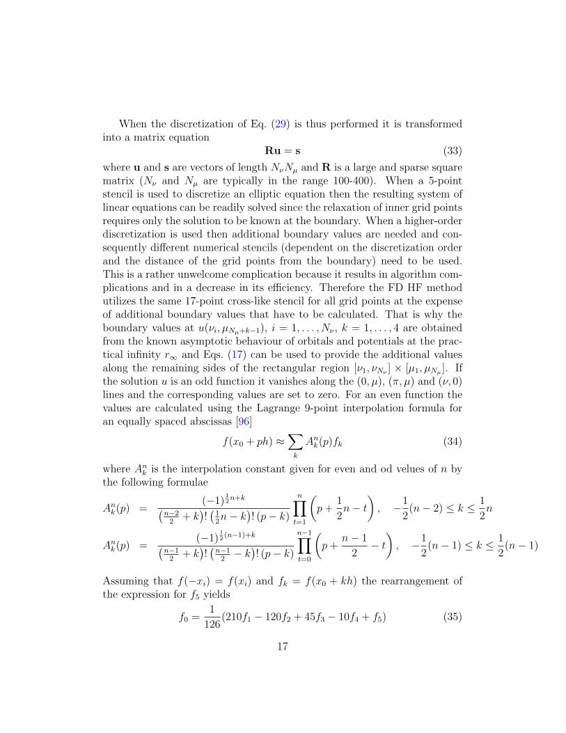
When the discretization of Eq. (29) is thus performed it is transformedinto a matrix equation

Ru = s (33)

where u and s are vectors of length NνNµ and R is a large and sparse squarematrix (Nν and Nµ are typically in the range 100-400). When a 5-pointstencil is used to discretize an elliptic equation then the resulting system oflinear equations can be readily solved since the relaxation of inner grid pointsrequires only the solution to be known at the boundary. When a higher-orderdiscretization is used then additional boundary values are needed and con-sequently different numerical stencils (dependent on the discretization orderand the distance of the grid points from the boundary) need to be used.This is a rather unwelcome complication because it results in algorithm com-plications and in a decrease in its efficiency. Therefore the FD HF methodutilizes the same 17-point cross-like stencil for all grid points at the expenseof additional boundary values that have to be calculated. That is why theboundary values at u(νi, µNµ+k−1), i = 1, . . . , Nν , k = 1, . . . , 4 are obtainedfrom the known asymptotic behaviour of orbitals and potentials at the prac-tical infinity r∞ and Eqs. (17) can be used to provide the additional valuesalong the remaining sides of the rectangular region [ν1, νNν ] × [µ1, µNµ ]. Ifthe solution u is an odd function it vanishes along the (0, µ), (π, µ) and (ν, 0)lines and the corresponding values are set to zero. For an even function thevalues are calculated using the Lagrange 9-point interpolation formula foran equally spaced abscissas [96]

f(x0 + ph) ≈∑k

Ank(p)fk (34)

where Ank is the interpolation constant given for even and od velues of n bythe following formulae

Ank(p) =(−1)

12n+k(

n−22

+ k)!(

12n− k

)! (p− k)

n∏t=1

(p+

1

2n− t

), −1

2(n− 2) ≤ k ≤ 1

2n

Ank(p) =(−1)

12

(n−1)+k(n−1

2+ k)!(n−1

2− k)! (p− k)

n−1∏t=0

(p+

n− 1

2− t), −1

2(n− 1) ≤ k ≤ 1

2(n− 1)

Assuming that f(−xi) = f(xi) and fk = f(x0 + kh) the rearrangement ofthe expression for f5 yields

f0 =1

126(210f1 − 120f2 + 45f3 − 10f4 + f5) (35)

17

Hence one can treat all the inner mesh points on an equal footing and performthe discretization of Eq. (29) by means of a single pair of numerical stencilsas defined by Eqs (31).

Since R matrix is large and sparse an iterative method must rather beused to solve the system of linear equations. In case of the FD HF methodorbitals and potentials are solved using the successive overrelaxation method(SOR) and its multicolour variant (MCSOR) which is better suited for vectorprocessors [31, 36, 94] (see also sec. 3.5, p. 27 and sec. 5.1, p. 35). Thestandard discretization of Eq. (29) by the second-order cross-like stencilsand the natural row-wise ordering of grid points (bottom to top, left toright) leads to a tridiagonal matrix with fringes [94]. The SOR method canbe used to solve such a system and the method is guaranteed to converge ifthe matrix R is symmetric, positive definite and the relaxation factor, ω, iswithin the interval 0 < ω < 2 [97, 94]. The (n+ 1)-th iterate of u is obtainedas

Rppu(n+1)p = (1−ω)Rppu

(n)p −ω

(p−1∑q=1

Rpqu(n+1)q +

NνNµ∑q=p+1

Rpqu(n)q − sp

), p = 1, . . . , NνNµ

(36)Assuming the natural rowwise ordering of grid points let us write Eq. (36)without explicit reference to matrix R. Applying the idea of the SOR methodto Eq. (29) discretized by formulae of Eq. (31) we have

G(νi, µj)u(n+1)(νi, µj) = (1− ω)G(νi, µj)u

(n)(νi, µj) + ωF (νi, µj)

−ωr/2∑k=1

[A(νi, µj)d

(νν)k

(u(n+1)(νi−k, µj) + u(n)(νi+k, µj)

)+B(νi, µj)d

(ν)k (u(n+1)(νi−k, µj) + u(n)(νi+k, µj))

+C(νi, µj)d(µµ)k (u(n+1)(νi, µj−k) + u(n)(νi, µj+k))

+D(νi, µj)d(µ)k (u(n+1)(νi, µj−k) + u(n)(νi, µj+k))

]where

G(νi, µj) = A(νi, µj)d(νν)r/2+1 + C(νi, µj)d

(µµ)r/2+1 + E(νi, µj) (37)

18

and i = 2, . . . , Nν − 1, j = 2, . . . , Nµ− 1, i.e. only the interior grid points arerelaxed (see also Sec. (5.1), p. 31).

The convergence of the SOR method depends critically on the value of theoverrelaxation parameter ω as shown in Table A.1. For a Poisson equationdiscretized by the second-order stencil one can show that the optimum valueof the overrelaxation parameter ωopt is given by the formula [94]

ωopt(Nν , Nµ) =2

1 +√

1− ρ(Nν , Nµ)2(38)

where ρ(Nν , Nµ) is the spectral radius of the corresponding matrix and isequal to cos(π/Nν)/2 + cos(π/Nµ)/2. There are no analogous results forhigher-order discretizations and for general elliptical second-order partial dif-ferential equations like Eq. (29) that must be solved to obtain orbitals andpotentials of the FD HF method. However, it has been shown that the (near)optimal value of the overrelaxation parameter for orbitals and potentials canbe approximated by the formula:

ωopt(Nν , Nµ) =2A

1 +√

1− ρ(Nν , Nµ)2+B (39)

where A and B are determined from numerical experiments [98]. In order toreliably determine ωopt for, say, orbitals, the potentials must be kept frozenand vice versa. The actual optimal values of the overrelaxation parametersused by the FD HF program are somewhat smaller since usually both orbitalsand potentials are relaxed in every SCF iteration and as a consequence thefunctions E(ν, µ) and F (ν, µ) also change.

3.2. Numerical differentiation and integration

Since the differentiation operator in µ and ν directions are independent,the differentiation over these variables can be performed separately. Thedifferential operator in the µ-direction reads

D(µ)f(ν, µ) =

(∂2

∂µ2+

ξ√ξ2 − 1

∂

∂µ

)f(ν, µ) =

(∂2

∂µ2+ ξ(µ)

∂

∂µ

)f(ν, µ).

(40)Let

df

dµ(νi, µj) =

4∑k=−4

d(1µ)k f(νi, µj+k) (41)

19

d2f

dµ2(νi, µj) =

4∑k=−4

d(2µ)k f(νi, µj+k) (42)

where d(1µ)k and d

(2µ)k are defined by Eq. (32) and Eg. (32), respectively. To

define D(µj)f(νi, µj) we write

D(µj)f(νi, µj) =4∑

k=−4

[d(2µ)k + ξ(µj)d

(1µ)k ]f(νi, µj+k) =

4∑k=−4

f(νi, µj+k)dkµ(µj)

= (fµj dµj

)i, µj+k = µj + khµ. (43)

where fµj matrix is (virtually) built from the 9 consecutive columns of fbeginning with the (j − 4)th column and dµj is the jth column of the arraydµ, i.e. (dµ)kj = dk

µ(µj). Thus evaluation ofD(µj)(νi, µj) for all ν values (i =

1, 2, . . . , nν) can be performed via a single matrix times vector multiplication(cf. routine diffmu).

The differentiation in ν-direction is performed analogously and the dif-ferential operator in the ν-direction reads

D(ν)f(ν, µ) =

(∂2

∂ν2+

η√1− η2

∂

∂ν

)f(ν, µ) =

(∂2

∂ν2+ η(ν)

∂

∂ν

)f(ν, µ).

(44)In the finite difference matrix representation it becomes

D(νi)f(νi, µj) =4∑

k=−4

f(νi+k, µj)dkν(νi) = (fνidνi)j, νi+k = νi + khν (45)

where fνi matrix is build from the 9 consequitive columns of fT (the trans-posed f matrix) beginning with the column i− 4 (cf. routine diffnu).

The integrals are evaluated using a two-dimensional generalization of 7-point one-dimensional integration formulae∫ x7

x1

dxf(x) =h

140(41f1 +216f2 +27f3 +273f4 +27f5 +216f6 +41f7)+O(h9)

(46)The two-dimensional integration weights are obtained as an outer productof the integration weights listed in Eq. (46). The order of the integration

20

formula determines the number of grid points in both directions. In thecase of the 7-point integration formula the number of grid points in ν and µdirection has to be of the form 6n+ 1.

The discretized orbitals and potentials can be represented as two-dimensionalarrays f such that fij = f(νi, µj), i = 1, . . . , Nν , j = 1, . . . , Nµ, νi = (i− 1)hνand µj = (j−1)hµ. Employing the two-dimensional integration formula thatcan be derived from Eq. (46) one can write

∫ π

0

dν

∫ µ∞

0

dµJ(ν, µ)f(ν, µ) =Nν∑i=1

Nµ∑j=1

cicjf(νi, µj)J(νi, µj) (47)

=Nν∑i=1

Nµ∑j=1

cijfij =

NνNµ∑k=1

ckfk,

k = (j − 1)Nν + i (48)

where c is a one-dimensional array of the integration weights merged withthe Jacobian and f is a two-dimensional array of f(νi, µj) values which istreated as a one-dimensional array. Thus the integral can be evaluated as adot product of the two vectors c and f and the integrals defined by Eqs. (24),(26), (27), (28) can be dealt with straightforwardly.

3.3. SCF and SOR iteration patterns

The salient feature of the finite difference Hartree-Fock method is the factthat the self consistent field iterative process of the Hartree-Fock methodand the successive overrelaxation iterations needed to solve the equationsare tightly interwoven. A certain number of successive overrelaxation itera-tions is carried out to update the values of orbitals and potentials betweentwo successive self consistent field iterations when the orbital energies arerecalculated, the orbitals reorthogonalized and the boundary values at µ∞reevaluated (the remaining boundary values are updated at every SOR iter-ation). Note that because of the iterative nature of the SOR method at nosingle SCF iteration the set of approximate linear equations is solved exactly(and it need not be). The accurate solutions (up to round-off errors) of theset of the linear equations and thus the Hartree-Fock equations are only ob-tained when the SCF/SOR process converges (the convergence depends onthe electronic configuration of a system, the initial estimates of orbitals andpotentials and the parameters used during the SOR iterations).

21

When performing calculations for a N-orbital atomic or diatomic system asingle SCF iteration requires the relaxation of N Fock equations to obtain theorbitals, N Poisson equations for the Coulomb potentials and about N2/2 –for the exchange potentials. For example, in case of the GaF molecule in eachSCF iteration one has to relax 2×15 equations for orbitals and Coulomb po-tentials and 120 equations for the exchange potentials. It has been observedthat 65-90% of the CPU time devoted to a given case is spent relaxing orbitalsand potentials and that the rate of convergence of the SCF process is mainlydetermined by the convergence behaviour of these relaxations. That is whythe proper choice of the overrelaxation parameters ωorb and ωpot is so impor-tant for the efficiency of the FD HF approach. It also effects the patternsof SCF convergence process. Figures (A.2) and (A.3) show the convergenceof the individual FH orbitals when some rather suboptimal overrelaxationparameters are used (ωorb = 1.65 and ωpot = 1.68). Initial estimates of theorbitals and potentials are crude and it takes several hundred iterations forthe SCF process to settle (about 250 for the 1 σ orbitals and twice as muchfor the 2 σ one). The convergence is exponential and the rate is nearly con-stant over the next ten thousand iterations. Only in case of the 2 σ orbitaland just after 6000 iterations one can notice a sudden variation in the rateof convergence which lasts for about 500 iterations. It must be kept in mindthat in each SCF iteration every orbital and potential undergos by defaultten SOR sweeps. It means that at no single SCF iteration we are seeking anexact (within roundoff errors, of course) solutions of the Poisson equationsfor orbitals and potentials. Instead, due to the iterative nature of the SORmethod the solutions are gradually improved.

When a near optimal parameter is used for orbitals and potentials, namelyωorb = 1.950 and ωpot = 1.989, the smoothing out of the convergence pat-tern takes about 750 SCF iterations but the convergence is six times faster;see Fig. A.4 and Fig. A.5. Because of this sort of behaviour it is not rec-ommended to use near optimal values of overrelaxation parameters at theonset of SCF process when initial estimates of orbitals and potentials arepoor as it may easily cause SCF process to go astray. Instead one shouldrather use conservative values for the overrelaxation parameters for a coupleof hundered iterations, save the orbitals and potentials and then restart theprogram with these functions as good initial estimates and the near optimalωorb and ωpot parameters to speed up the relaxation process. A similar over-all convergence pattern can be seen by ploting the total energy differencescalculated every tenth SCF iteration as shown in Fig. A.6.

22

The number of sweeps that are performed for every single function under-going relaxation is an adjustable parameter and can be set within the range10-40 without drastically changing the convergence rate. Table A.2 shows thedependence of the total number of SOR iterations and the time required tosolve the FD HF equations on the number of SOR iterations applied to relaxorbitals and potentials in a single SCF iteration. The problem has not beenthroughly examined but it seems that the optimum value of this parametercannot easily be found and the net effect may not be worth the effort.

3.4. Accuracy of the method

The FD HF method is a truely basis-set-independent approach and ifthe mesh and r∞ are chosen adequately the HF orbitals can be obtained tothe required accuracy (within double or quadruple precision arithmetic). Inorder to see this let us consider the Fock equation for an orbital φ (a subscriptis omitted for readibility) at a given SCF iteration, i.e. we assume that theFock operator does not depend on its eigenfunctions

Fφ = Eφ

where

φ =∞∑i=1

ciχi

is expanded into a complete set of orthonomal basis functions χi. When afinite basis set is used an approximate solution is written as

φ =M<∞∑i=1

ciχi

and the Fock equation is transformed into an approximate one

Fφ = Eφ

One can writeφ = φ+ ∆φ (49)

where the truncation error ∆φ is orthogonal to φ or otherwise ∆φ would

be included in φ. However,⟨φ∣∣∣ ∆φ

⟩= 0 + δroundoff , i.e. the orthogonality

condition is limited by the degree of the linear dependence within a given

23

basis set which is directly related to accuracy of floating-point arthmetic(δroundoff). Therefore

E = 〈φ|F |φ〉 = E + 2δroundoffE + 〈∆φ|F |∆φ〉

Usually when algebraic method is employed to solve the Fock equations theroundoff errors are much smaller than basis set truncation errors. Hencethe orbital energies are calculated to a higher accuracy than the orbitalsthemselves and that is the reason why the calculation of properties are oftenregarded as a much more sensitive test of the quality of a given basis thanthe total energy alone.

When the finite difference solution of the Fock equation is attemptedEq. (49) can still be used but one can no longer assume that φ and ∆φ areorthogonal since now the orbital error is due to both roundoff and discretiza-tion errors. When calculations are carried out in double precision arithmeticthe former are (usually) much smaller than the latter. The accuracy of theenergy can be increased by changing the grid size as long as the discretizationerrors are larger than the roundoff ones. Thus⟨

φ∣∣∣ ∆φ

⟩= 0 + δdiscr + δroundoff , δdiscr � δroundoff

and the orbital φ can only be normalized up to the discretization errors.Therefore

E = 〈φ|F |φ〉 = E + 2δdiscrE + 〈∆φ|F |∆φ〉i.e. the orbital energy error depends linearly on the orbital error which, in thiscase, is mainly due to the discretization. If the changes of the Fock operatorduring the SCF process were taken into account the error analysis would bemore complicated. However, the linear dependence of the total energy ondiscretization errors can still be observed as the data for the hydrogen andhelium atoms collected in Tables A.3 and A.4 show.

The approximate character of 1 σ orbital can be well monitored by cal-culating the total electronic dipole moment (along the z-axis) of the system.Clearly, the accuracy of the total energy as measured by the error of thevirial ratio closely matches the quality of the orbital. And in this particularcase the grids larger than [151× 193/25] cannot improve the solution of theHF equation.

In order to obtain accurate solutions of the FD HF equations one hasto quarantee that both a single orbital and a single Coulomb or exchange

24

potential are calculated to a high and comparable accuracy. Let us examinesolutions of the Fock equations first. Table A.5 contains eigenvalues of sev-eral σ, π, δ and ϕ states of the GaF+39 system obtained by solving the Fock(Schrodinger) equation by means of the FD method together with the corre-sponding values obtained from Power’s program that generates eigenvaluesfor the bare-nuclei one-electron diatomic systems [99, 100]. The agreementis perfect and small discrepancies can be attributed to inevitable roundofferrors.

The overall quality of the FD HF method for diatomics can be examinedby applying it to an atomic system that can be described by a single Slaterdeterminant (especially a closed-shell one) since the numerical HF results foratoms are readily available. Table A.6 shows the orbital and the total energiesof the calcium atom obtained by means of the modified finite difference one-dimensional HF program of Froese Fischer [93, 101] and its two-dimensionalcounterpart (the internuclear separation between the atom and its nonexis-tent partner, i.e. a centre with no charge, was set to 2 a.u. since such achoice of the separation guarantees that similar grids are used when solvingthe FD HF equations for the atom and the diatomic molecule). This compar-ison demonstrates that the accuracy of the two methods matches very well.This level of agreement can only be obtained when the one-dimensional gridis large enough and carefully chosen (one has to adjust the ρ0 and h param-eters which determine the first non-zero value of the radial variable and thestep size, respectively). Both programs can deliver total energies that have12-13 significant figures and it seems that this is the ultimate accuracy thatcan be expected from finite difference programs that use double precisionarithmetics for floating-point operations. Since the FD HF program treatsatomic and diatomic systems on an equal footing, we expect that the samelevel of accuracy can be obtained when solving the HF equations for diatomicmolecules. That this is indeed the case, can be seen from Table A.7 wherethe total HF energies of the the beryllium atom and for the LiH, BH andN2 molecules calculated by means of the FD and a multigrid finite elementmethods are compared. The highly accurate finite element results correspondto the extrapolated values obtained from a series of calculations performedon grids of increasing density [21].

3.5. Efficiency of the method

The analysis of numerical complexity of the three alternative methods ofsolving the HF equations for diatomic molecules, i.e. PWSCF, FD and FE,

25

show that the FD method is about ten-fold more efficient than the other ap-proaches [39]. This is mainly due to the fact that in the FD method the SCFiterations are interwoven with only a small number of SOR relaxation sweeps.This means that in a given SCF iteration the Fock and Poisson equations arenot solved exactly by the SOR method but that the solutions are graduallyimproved and one gets the correct solution only upon the convergence of boththe SCF and SOR iterations. Various improvements introduced into the FDHF method in the course of its development have resulted in considerableincrease in its efficiency and therefore this method can be applied routinelyto small- and medium-size diatomic molecules. Of course, as a result of theconstant enhancement in computers’ performance the notion of the medium-size molecule refers to the larger and larger systems: a decade ago to thesystems containig about 10-15 electrons, nowadays – 35-45.

The program allocates memory according to a case under consideration,i.e. the requested number of orbitals and the grid size. This means thatthe same binary version of the program can be used for systems of variablesizes, or calculation for a given system may be performed with an increasingaccuracy.2 The solutions can be transfered between grids of different densi-ties which greatly simplifies performing calculations for a series of grids ofincreasing density.

In the FD HF method the orbital and the potential functions u(ν, µ) arediscretized on the rectangular region using meshes with Nν and Nµ points inthe respective variables. The partial differential equations of the HF methodin the form of Eq. (29) are discretized using the 8th-order central differenceexpressions given by Eqs. (32) and (32) which yield a 17-point cross-likestencil. The use of the 17-point numerical stencil instead of its 13-pointcounterpart that was employed in the original version of the method [31] todiscretize the HF equations resulted in the decrease of the truncation errorsby two orders of magnitude (from O(h6) down to O(h8)). Thus the numberof the grid points could be reduced by half without impairing the qualityof the solution.3 The usage of the higher-order discretization stencil has tobe matched with increased accuracy of the numerical integration routines.Therefore, the 5-point (composite) numerical integration was replaced by its

2There are some hard-coded arrays and their dimensions must be adjusted duringcompilation of the program; see INSTALL file of the x2dhf package.

3In case one solves a model Poisson equation the savings due to the higher-order dis-cretization can be even larger.

26

7-point equivalent. The accuracy of the boundary values for the orbitals andpotentials at the practical infinity, r∞, were also increased, which allowed todecrease this value and reduce the grid size while retaining the overall accu-racy. The program was to be used on Cray and Convex computers utilizingvector processors. To make use of this important feature all parts of theprogram essential for its efficiency were cast in vector-vector, matrix-vectorand matrix-matrix form and perfomed by means of the BLAS library rou-tines. This approach proved also advantageous when the program is usedon modern superscalar architectures with the BLAS library routine support[102]. Upon the introduction of these changes it has turned out that theefficiency of the FD HF method depends solely on the efficacy of the methodused to solve the systems of linear equations. That is why some effort hasbeen put into the careful implementation of the SOR method (and its mul-ticolour variant) [36]. With the 17-point numerical stencil the relaxation ofa single grid value requires 56 floating point operations and the process canbe performed with the speeds of about 1 and 2 GFLOPS for AMD Opteron2200 (2.8 GHz) and Intel E8400 (3 GHz) processors, respectively.

4. ONE-ELECTRON POTENTIALS

The primary application of the FD HF method is of course solving theFock equations for diatomic molecules. However, with some modificationsit can also be used to solve this sort of two-dimensional partial differentialequations with other one- and two-particle attractive potentials.

4.1. DFT potentials

In particular, the FD HF method can be used to solve the Fock equa-tions with various density functional potentials. The program supports theLDA and B88 [103] local exchange potentials and the LYP [104] and VWN[105] correlation potentials; the corresponding formulae for potentials andenergies together with the relevant references can be found in Appendix Ap-pendix A, p. 41. Table A.8 contains comparison of total energies of the He,Be and Ne atoms calculated within the finite basis set and finite differenceapproaches with various combinations of local exchange (LDA and B88) andcorrelation potentials (LYP and VWN). The present version of the FD HFprogram can be used to perform calculations by means of the self-consistentmultiplicative constant method of Karasiev and Ludena [87] where the Xα

27

exchange potential is used with the α parameter adjusted in every SCF iter-ation (cf. Table A.9, A.10). The program also allows to calculate LDA, B88,PW86, PW91, LYP and VWN contributions to the total energy for any setof orbitals. It is worth mentioning that automatically adjusted values of therelaxation parameters ωorb and ωpot should be avoided when using the localexchange potentials. In such instances one should set these parameters to(sometimes much) smaller values in order to guarantee the convergence ofthe SCF/SOR process.

The LDA (Xα) approximation is often used as a handy way of generatinggood initial estimates of orbitals. In such a case the recommended α valuesfor elements from helium to niobium are taken from Schwarz [106] and areextrapolated for the remaining ones. To this end one can also use the modelpotential of Green, Sellin and Zachor [107]. For a given atom this potentialproduces HF-like orbitals and was found useful in finding decent startingorbitals for any molecular system.

4.2. Krammers-Henneberger potential

The FD HF program can also be employed to solve the Schrodinger equa-tion for a one-electron diatomic system with an arbitrary but binding poten-tial and it can be treated as a finite difference solver of the Schrodinger equa-tion for the three-dimensional potential in cylindrical coordinates [92]. Thepresent version of the program supports the (smoothed) Coulomb potential

V =−V0√a2 + r2

=−V0√

a2 + x2 + y2 + z2

and the Krammers-Henneberger potential

V =−V0

2πω

√a2 + b2

x + y2 + z2

with bx = x+α0 +α0(cos(ωt)−1), α0 = E0/ω2 and where a is a width of the

model potential, V0 – its depth, E0 – the laser field intensity, ω – its cyclefrequency.

4.3. Finite field approximation

For diatomic molecules z-components of polarizabilities and hyperpolar-izabilities can be evaluated by the finite field approximation when the field

28

is applied along the internuclear axis. The effect of this field is attributed byadding terms of the form

−∑i

µiz(0)Fz (50)

to the hamiltonian where µiz(0) is the z-component of the permanent dipolemoment for the i-th electron. The induced dipole and quadrupole momentscan be written as the expansions [108, 109]

µz(Fz) = µz(0) + αzzFz +1

2βzzzF

2z +

1

6γzzzzF

3z + · · ·

Θzz(Fz) = Θzz(0) + Az,zzFz +1

2Bzz,zzF

2z + · · · (51)

When the moments are evaluated for 0, ±F 0z and ±2F 0

z values of the field the5-point central difference approximations to the derivatives can be employedresulting in the following approximate formulae for the dipole polarizabil-ity (αzz), the first and second dipole hyperpolarizabilities (βzzz and γzzzz),the dipole-quadrupole polarizability (Az,zz) and the dipole-dipole-quadrupolehyperpolarizability (Bzz,zz):

αzz =

(dµzdFz

)Fz=0

≈ µz(−2F 0z )− 8µz(−F 0

z ) + 8µz(+F0z )− µz(+2F 0

z )

12F 0z

βzzz =

(d2µzdF 2

z

)Fz=0

≈ −µz(−2F 0z ) + 16µz(−F 0

z )− 30µz(0) + 16µz(+F0z )− µz(+2F 0

z )

12(F 0z )2

γzzzz =

(d3µzdF 3

z

)Fz=0

≈ −µz(−2F 0z ) + 2µz(−F 0

z )− 2µz(+F0z ) + µz(+2F 0

z )

2(F 0z )3

(52)

Az,zz =

(dΘzz

dFz

)Fz=0

≈ Θzz(−2F 0z )− 8Θzz(−F 0

z ) + 8Θzz(+F0z )−Θzz(+2F 0

z )

12F 0z

Bzz,zz =

(d2Θzz

dF 2z

)Fz=0

≈ −Θzz(−2F 0z ) + 16Θzz(−F 0

z )− 30Θzz(0) + 16Θzz(+F0z )−Θzz(+2F 0

z )

12(F 0z )2

In principle, the polarizability and the first hyperpolarizability can alsobe evaluated as the second and the third derivatives of the total energy withrespect to the field, i.e.

αzz = −(d2E

dF 2z

)Fz=0

βzzz = −(d3E

dF 3z

)Fz=0

(53)

29

and approximated by the above finite differences accordingly. However, thisapproach is less preferable as it requires the total energy values of very highquality to be applied in a numerically stable fashion. The calculations of (hy-per)polarizabilities by means of Eqs (52) seems to be a straightforward pro-cedure but it also requires very accurate values of the dipole moment, espe-cially when the second dipole hyperpolarizability values are of interest. Thisis readily seen from Table A.11 where the values of the total energies and thedipole and quadrupole moments of the hydrogen fluoride obtained for fivedifferent values of the electric field are examined. The upper part of the ta-ble contains raw data extracted from the program’s listings by a Perl script.4

This script uses Eqs (52) to evaluate the polarizabilities and hyperpolariz-abilities from the supplied data. A careful examination of the SCF/SORiteration process shows that the total energies and multipole moments areknown with the relative error of the order 10−12. This information can alsobe supplied to the script and the dependence of the electric properties onthe quality of the solution estimated. It is worth noting that even the dipolemoment calculated by taking the first derivative of the energy has at most4 correct figures and as a consequence leads to the polarizability with only2 significant figures. The value of the first hyperpolarizability is completelyuseless. By contrast the dipole moment calculated from orbitals inheritstheir accuracy and even the second hyperpolarizability can be quoted with3-4 figures.

The problems with the finite field approach are twofold. First, if theFD HF equations with the hamiltonian modified by the presence of the ex-ternal field are solved, the chosen field strength must be small enough toyield converged and numerically stable results. The presence of the externalelectric field makes it more difficult to apply boundary conditions at infin-ity. In fact, much larger values of the practical infinity (up to 150-200 bohr)must be chosen in order to converge the SCF/SOR process to high accuracy.As a result, the number of grid points required is increased thereby raisingthe computational demands of the FD HF calculations, which are alreadymultiplied by the factor of 5 because of the 5-point difference formulae usedto calculate (hyper)polarizabilities. Second, the field must be strong enoughto facilitate meaningful numerical differentiation of the dipole moment values

4The listings and the script can be found in examples/fh and utils subdirectories of thex2dhf package, respectively.

30

for different field strengths. Since it may be difficult to satisfy both require-ments, the FD HF equations are usually solved on a number of different gridsand with several field strengths.

Recently this approach has been used to calculate accurate values of po-larizabilities and hyperpolarizabilities for atoms, hetero- and homonucleardiatomic molecules and their ions [55, 56]. The dependence of these proper-ties on the internuclear separation can also be studied as Table A.12 shows.Calculations for atoms and heteronuclear molecules are rather straightfor-ward once the grid is chosen. However, homonuclear systems pose a problemsince a weak external electric field breaks the inversion symmetry and theSCF/SOR iteration process fails to deliver well converged solutions. It hasrecently been shown that the problem encountered is due to a near degener-acy of some of its orbitals and can be circumvented by allowing for non-zerooff-diagonal Lagrange multipliers between such orbitals. The modified FDHF method was used to perform calculations of electrical properties for theH2, Li2, F2, N2 and O2 molecules and the results can be found in [56]. Thequality of the properties can be assessed by the examination of the resultsfor the N2 molecule shown in Table A.13. The values of the polarizabilityand the first hyperpolarizability should be compared with the best algebraicHF values obtained to date by Maroulis, namely 15.0289 and 799 [110].

4.4. Finite nuclei

The FD HF program is also suited to study atomic and diatomic systemswith the finite nuclei. The charge distribution within a nucleus can be de-scribed by either Gaussian and Fermi models [91] where parameters definingthe atomic masses of the nuclei are taken from the table of atomic massescompiled by Wapstra and Audi [111, 112] (see Appendix Appendix A, p. 49,for details).

5. DESCRIPTION OF THE CODE

5.1. Structure of the code

It is assumed that the reader has unpacked the program’s package andhas access to the User’s Guide pdf file that can be found in docs directory.

The large scale structure of the program is presented in Fig. A.7.5 The

5The x2dhf package contains the file ftnchek html/CallTree.html which can be usedto browse the complete call tree of the program.

31

main routine x2dhf is shown calling the twelve first level routines in theorder given, i.e. printBanner is invoked before setPrecision, setDefaults andso forth. The routines of the second and third levels are also given and if theircalling order is irrelevant they are put into a box. The program starts byprinting its name and version. Then it determines the lengths of integer andfloating-point constants and variables since the program can be compiled tosupport calculations using three different combinations of integer/real datatypes: i32 (4-byte integers, 8-byte reals), i64 (8-byte integers, 8-byte reals)and r128 (8-byte integers, 16-byte reals); see src/Makefile for details. Thesevalues are used for seamless retrieval of binary data when reading orbitals andpotentials from disk files. In some cases, especially when quadruple precisoncalculations are attempted, this is not enough because of non-standard dataformats employed by Fortran compilers. In such cases it is recommended toexport and import data in formatted instead of unformatted form (see inoutlabel). Next the default values of various scalar and array variables are setand the program is ready to read input data. The retrieval of input data iscontrolled by inputData routine and inCard routine is used to read a singleline at a time and scan it in search for nonspace fields (if an exclamationmark or a hash is found then whatever follows is treated as a comment).Subsequently inStr, inInt and inFloat routines are used to extract string,integer and floating-point data, respectively. The input must contain atleast the following cards: TITLE, NUCLEI, GRID, CONFIG, ORBPOT andSTOP. TITLE gives at most 80 character-long description of a given case andis used as a label of disk files with orbitals and potentials. NUCLEI carddefines the charges of atoms A and B and their separation (in atomic units orangstroms). The grid is specified by providing at least the number of pointsin the ν variable (Nν) and the practical infinity (r∞). The number of pointin the µ variable (Nµ) is then subsequently calculated so that the step sizesin both the variables are approximately the same to guarantee a comparablelevel of truncation errors when performing differentiation and integration offunctions. Additionally, Nν and Nµ are adjusted to the form 6k + 1 sincethe numerical integration is based on a 7-point integration formula. If themulticolour SOR method is used then Nν must be further restricted to theform 5k + 6 in order to subdivide the mesh points into five independentsubsets.

The program uses fixed-size common blocks and variable-length arrays tomove data between routines. However, the size of some common block arraysis determined during the compilation through MAXNU and MAXMU vari-

32

ables (see src/Makefile.am). These variables set the maximum number of gridpoints in ν and µ variables, respectively, that can be used when specifying thegrid size for a given case. The size of the variable-lenghth arrays is howevercase dependent and the C routine memAlloc is used to allocate the requiredspace. Now initArrays is called to perform initialization of various com-mon block variables and common block and variable-length arrays. First ofall the subroutine initCBlocks initializes grid, orbital and SOR data. TheninitAddr is called to calculate dimensions of variable-length arrays cw orb,cw coul, cw exch for holding orbitals, Coulomb and exchange potentials andto calculate their respective addresses within these arrays. cw suppl array isalso partitioned and the routine initSuppl is called to initialize arrays forone-electron potentials, integration weights and Jacobians for one- and two-particle integrations, etc. initMesh is responsible for establishing an order ofmesh points. By default the ’middle’ type of ordering is chosen but the natu-ral column-wise, row-wise and the reverse natural column-wise orderings canalso be selected (see below). Finally initExWeights calculates the weightsof exchange contributions to the (restricted) open-shell Hartree-Fock energyexpression. Now, when the input data are processed the relevant informationabout the way the given case will be handled can be printed (printCase).One can thus check the method that will be applied, the electronic configura-tion defined and the grid, SCF and SOR parameters. The detected machineaccuracy, the values of the π constant and the bohr to angstrom conversionfactor together with the summary of memory usage are also printed.

Before the SCF process can begin the initial values of orbitals and Coulomband exchange potentials must be provided. The molecular orbitals can beformed as a linear combination of either atom-centred hydrogen-like orbitals(via LCAO label, see initHyd) or numerical orbitals taken from the atomicHF program (see initHF). Good estimates of the molecular orbitals canbe obtained by means of the GAUSSIAN package when its appropriate outputfiles are provided (see mkgauss option of tests/xhf script). The Coulombpotentials are calculated using the Thomas-Fermi model and the exchangeones are approximated by 1/r (see initPot). Unless the LCAO cards arepresent the contributions from both the centres are taken with equal weights(in case one of the centres has zero nuclear charge the corresponding mixingcoefficient is also set to zero). Of course orbitals and potentials (togetherwith other relevant data) can be retrieved from disk files so that the currentcase can be treated as a continuation of a previous run of the program.

Now, the initial orbitals can be normalized and orthogonalized and the

33

evaluation of diagonal and off-diagonal Lagrange multipliers can follow (seeprepSCF). The multiple moments and the total energy are also calculatedand the program proceeds to its core doSCF routine (see Fig. A.8). Therethe already calculated multipole moments are used to determine boundaryvalues of Coulomb and exchange potentials at the practical infinity, r∞ (seepotAsympt), and the solution of the Poisson equations for potentials can beadvanced by perfoming several (10 by default) iterations of the SOR method(see coulSOR and exchSOR). This is done in the orbital loop for each orbitalin turn with the order determined by the electronic configuration as specifiedby input data, i.e. σ-type orbitals first, then π, δ and ϕ. For each orbital theupdated Coulomb and exchange potentials are used to construct the Fockequation, the boundary values of the orbital at r∞ are evaluated and theorbital values at the mesh points are updated by performing several SORiterations (see the discussion of orbSOR routine below). Then the orbital isnormalized and orthogonalized and the diagonal and, if needed, off-diagonalLagrange multiplies are recalculated. When all the orbitals are thus pro-cessed the convergence criteria are examined. If the SCF iteration limit isreached or the maximum changes of orbital energies and/or their norms meettheir respective thresholds the SCF/SOR iteration process terminates. Oth-erwise the next SCF iteration begins with the recalculation of the multipolemoments, if the changes in orbital energies between two consecutive SCFiterations are large enough.

A few more words are needed to clarify the algorithm used to performSOR iterations. Since the boundary values for the potentials are calculatedbefore calling the coulSOR and exchSOR routines these are only responsiblefor relaxing the function values. In Fig. A.9 the unnumbered star-like pointsrepresent these boundary values. In order to be able to use the same 17-pointcross-like stencil for the discretization of the Poisson equation for all (num-bered) grid points the function being relaxed is immersed in a larger grid.When the routine putin transfers this function from the original grid into itsextended counterpart it also sets the values at the bullit-like points using theeven or odd symmetry of the function. Now the relaxation can proceed in achosen given order of grid points (the column-wise in our example). Whenthe process is over the symmetry of the function can be used again to fix thevalues of ×- and ⊗-like grid points: for functions of even symmetry thesevalues are obtained from interpolation or set to zero otherwise (see sor rou-tine). The relaxation sweeps (together with the interpolation) are repeatedas many times as required and putout routine is used to transfter updated

34

function values from the extended grid to the original one. In the case oforbSOR routine the local and non-local parts of the Hartree-Fock potentialhas to be calculated first by calling fock routine (see Fig. A.10). Then theasymptotic behaviour of the Fock equation is used to determine parametersneeded to calculate the boundary values of orbitals at µ∞ (see orbAsymptDetand orbAsymptSet).

Fig. A.9 shows the column-wise ordering of mesh points. By defaulthowever, the x2dhf program uses the so-called middle-type ordering whichresults in a bit faster convergence of the SCF/SOR process. As shown inFig. A.11 the µ coordinates change according to the following order µ(M−1)/2,µ(M−1)/2−1, . . ., µ1, µM/2, µM/2+1, . . ., µM . For each µi the ν coordinates formthe sequence: ν(N−1)/2, ν(N−1)/2−1, . . ., ν1, νN/2, νN/2+1, . . ., νN , where M andN are number of grid points in each direction undergoing relaxation.

In case the multi-colour SOR is used all the mesh points undergoingrelaxation can be subdivided into five colours or colour suits as shown inFig. A.12 (the triangles denote the no trump). It can easily be seen thatwhen the 17-point stencil is used for descritization the relaxation of, say, theclubs points depend only on the values of points of remaining colours. Thatis why the points of the same colour can be relaxed simultaneously and thealgorithm can be vectorized resulting in a five-fold speedups. It is possible toparallelize the method within the OpenMP scheme but unfortunately no gainin efficiency could be obtained. It is hoped that the MCSOR algorithm can beeffectively implemented on general-purpose graphics processing units usingCUDA technology (http://www.nvidia.com/object/cuda home new.html).

In order to help to understand how the program works, a short descriptionof all its most important routines follows in lexicographic order.

inCard reads (and echoes) a single line of input data and scans it in searchfor nonspace fields. If an exclamation mark or a hash is found thenwhatever follows is treated as a comment. inStr, inInt and inFloat

routines are used to extract string, integer and floating-point data,respectively.

coulAsympt determines for a given orbital asymptotic values of the corre-sponding Coulomb potential

coulMCSOR prepares the right-hand side of the Poisson equation for a givenCoulomb potential and performs the default number of MCSOR itera-tions (cf. mcsor).

35

coulMoments determines the multipole expansion coefficients for Coulombpotentials

coulSOR prepares the right-hand side of the Poisson equation for a givenCoulomb potential and performs default number of SOR iterations (cf.sor). In order to be able to use the same numerical stencil for allgrid points putin and putout routines are used transfer the functionbetween the primary and extended grids.

doSCF controls the SCF process. In every SCF iteration orbitals are relaxedin the reverse order as defined by the input data. For a given orbital theboundary values of the corresponding Coulomb and exchange potentialsat r∞ are calculated and the functions are relaxed by performing severalSOR iterations. Then the boundary values of the orbital are evaluatedand the orbital undergoes SOR relaxations. Next, it is normalized andorthogonalized by means of the Schmidt algorithm. If required, theinversion symmetry of the orbital can also be imposed. Subsequently,its orbital energy and, if necessary, off-diagonal Lagrange multipliersare calculated. This same procedure is repeated for every (non-frozen)orbital. From time to time the mpoleMom routine is called and themultipole moments needed to evaluate asymptotic values of potentialsare recalculated. Also every declared number of SCF iterations thetotal energy is calculated and the orbitals and potentials are writtento disk. The SCF process is terminated if the convergence criteria aremet or the maximum number of SCF iterations is reached.

Ea computes the eigenvalue of the Fock equation for a given normalizedorbital as

Ea =< φa| − 12∇2 + Vn + VC − V a

x |φa >.

Eab computes the off-diagonal Lagrange multiplier for a pair of normalizedorbitals.

EaDFT computes the eigenvalue of the Fock equation for a given orbital whena local exchange approximation is used.

EabDFT computes the off-diagonal Lagrange multiplier for a pair of normal-ized orbitals in case a local exchange approximation is used.

Etotal evaluates the HF total energy.

36

EtotalDFT evaluates the total energy for a given DFT potential.

exchAsympt determines from the multipole expansion asymptotic (bound-ary) values of the exchange potentials entering a given Fock equation.

exchMCSOR prepares the right-hand side of the Poisson equation for a givenexchange potential and performs the default number of MCSOR itera-tions.

exchMom determines the multipole expansion coefficients for exchange poten-tials.

exchSOR prepares the right-hand side of the Poisson equation for a givenexchange potential and performs the default number of SOR iterations.

initArrays initializes various common blocks and variable-length arrays.

initAddr calculates dimensions of arrays and addresses of particular or-bitals, Coulomb and exchange potentials within dynamically allocatedarrays cw orb, cw coul, cw exch; arrays cw suppl and cw sctch are alsopartitioned.

initCBlocks checks and adjusts the requested dimensions of the grid andinitializes some common block arrays with grid, orbital and SOR data.

initDisk controls retrieving of orbitals and potentials together with someother data (Lagrange multipliers, multipole moment expansion coeffi-cients, etc.) from disk files in binary or ascii format.

initExWeights calculates the weights of exchange contributions to the (re-stricted) open-shell Hartree-Fock energy expression.

initGauss initializes molecular orbitals through the discretization of GAUS-SIAN orbitals reconstructed from the GAUSSIAN output (see prepGaussfor details); Coulomb and exchange potentials are initialized as ininitHyd.

initHF initializes molecular orbitals as a linear combinations of Hartree-Fock

37

orbitals on centres A and B (orbitals are generated by the qrhf pro-gram6); Coulomb and exchange potentials are initialized as in initHyd.

initHyd initializes molecular orbitals as a linear combinations of hydrogenicfunctions on centres A and B; Coulomb and exchange potentials areinitialized by calling initPot.

initMesh establishes ordering of mesh points (cf. order label).

initOrbPot initializes orbitals and potentials (see initHyd, initHF, prepGauss,initGauss, initDisk and initTF for details).

initPot initializes Coulomb potentials as a linear combination of the Thomas-Fermi potentials at the atomic centres. In case of HF calculations ex-change potentials are approximated as the corresponding linear com-bination of 1/r terms. In case of DFT calculations the local exchangeapproximation is used.

initSuppl initializes various supplementary arrays of case-dependent lengthssupported by cw suppl (one-electron potentials, Jacobians, integrationweights, etc.).

inFloat – see inCard.

inInt – see inCard.

inputData handles the input to the x2dhf program.

inStr – see inCard.

mcsor performs one iteration of the multicolour successive overrelaxationscheme.

memAlloc dynamically allocates memory acccording to grid requirementsand orbital configuration of the current case (a C routine).

memDealloc releases memory allocated by memAlloc (a C routine).

6This is a modified version of Fischer’s MCHF program that can be downloaded fromhttp://fizyka.umk.pl/˜jkob/qrhf.

38

mpoleMom determines the coefficients of the multipole expansion for Coulomband exchange potentials (see coulMom and exchMom).

norm performs normalization of a given orbital.

ortho performs the Schmidt orthonormalization of a given orbital.

orbAsymptDet initializes an array which is used by orbAsymptSet to calcu-late boundary values of a given orbital at practical infinity.

orbAsymptSet recalculates asymptotic values of a given orbital at the practi-cal infinity using exponential decay values prepared by calling orbAsymptDet.

orbMCSOR performs the same tasks as orbSOR but uses the MCSOR methodfor solving the Poisson equation (cf. mcsor).

orbSOR evaluates the Fock potential (cf. fock and fockDFT) for a givenorbital, sets up the right-hand side of the Poisson equation for thatorbital and performs a default number of SOR iterations (cf. sor). Inorder to be able to use the same numerical stencil for all grid pointsputin and putout routines are used to transfer functions between theprimary and extended grids. orbAsymptDet and orbAsymptSet areused to calculate boundary values.

potAsympt determines from the multipole expansion asymptotic (boundary)values of the Coulomb and exchange potentials needed for a given Fockequation.

prepGauss extracts basis set parameters from an output of the GAUSS-SIAN94/98 program (gaussian.out and gaussian.pun files) to be usedby initGauss routine.

prepSCF prepares the SCF process by orthogonalizing orbitals, calculationof orbital energies, evaluation of Lagrange multipliers and multipolemoment expansion coefficients.

printBanner prints the name and version of the program.

printCase outputs the information about the case being defined by theinput data (molecular system, internuclear separation, configuration,grid, memory requirements, etc.).

39

printResults outputs the results of calculations, i.e. the final total energytogether with its contributions, DFT values of Coulomb, exchange andcorrelation energies, orbital energies and normalization errors, multi-pole moments and CPU usage.

putin takes a function defined on the primary grid and immerses it intothe extended grid so that the same 17-point cross-like stencil can beused for the discretization of the Poisson equation for all grid pointsundergoing relaxation; the odd or even symmetry of the function isused to supply extra boundary values.

putout reverses the work of the putin routine and transfers a given functionvalues from the extended to primary grid.

setCi determines inversion symmetry of a given orbital (or set of orbitals)and sets its value at (ν, µ), where ν = π/2, . . . , π and µ = 1, . . . , µ∞ bythe corresponding values at ν = 0, . . . , π/2.

setDefaults sets default values of various scalar and array variables, in par-ticular those responsible for the ordering of mesh points and controllingthe SOR relaxations and the SCF process.

setPrecision calculates floating-point precision and the lengths of integerand real variables in order to handle input and output data and print-outs correctly. On x86 systems the precision depends on compiler op-timization flags used and therefore this routine must be compiled withthe minimum optimization in order to avoid reporting precision of theextended IEEE 754 arithmetic (see src/Makefile.am).

sor performs one iteration of the successive overrelaxation scheme.

writeDisk writes molecular orbitals, Coulomb and exchange potentials to-gether with some other data such as Lagrange multiplies, multipolemoment expansion coefficients etc. in binary format to disk files.

5.2. Language, features and limitations of the program

Except for two C routines used to allocate and deallocate memory theprogram has been written in Fortran 77. Fortran 95 can also be used tocompile the program but no specific features of this version of the languageare used. The program uses the date and time library routine for retrieving

40

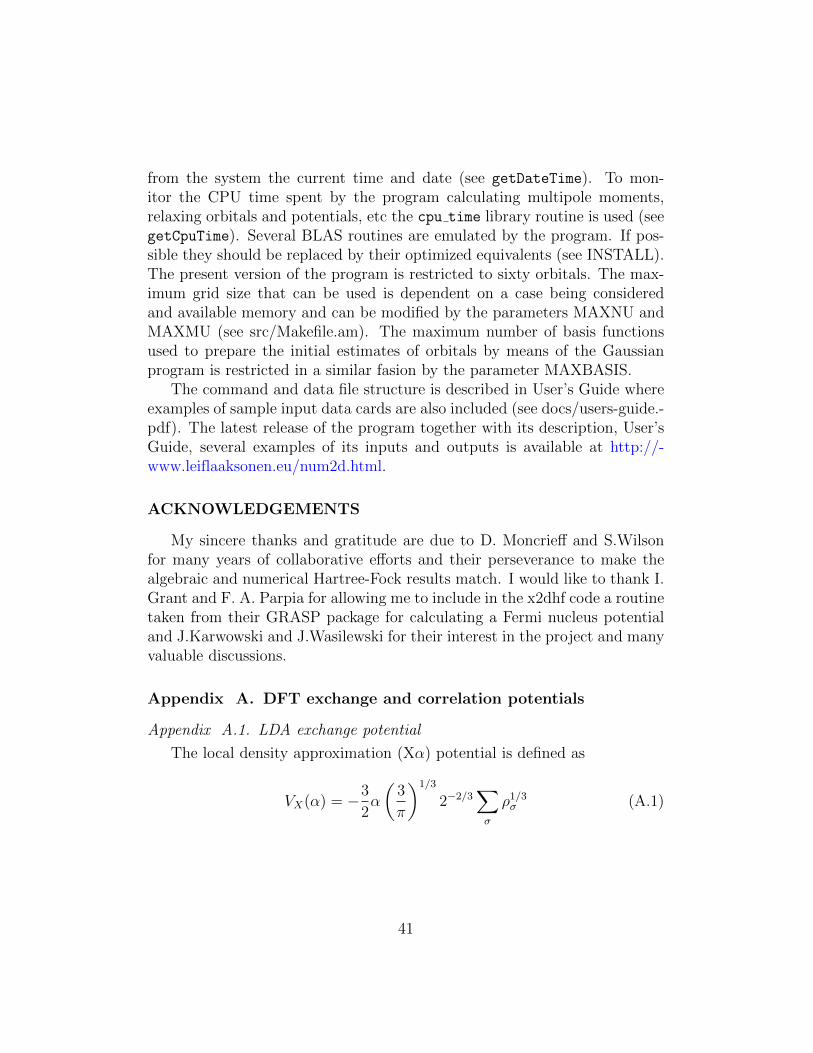
from the system the current time and date (see getDateTime). To mon-itor the CPU time spent by the program calculating multipole moments,relaxing orbitals and potentials, etc the cpu time library routine is used (seegetCpuTime). Several BLAS routines are emulated by the program. If pos-sible they should be replaced by their optimized equivalents (see INSTALL).The present version of the program is restricted to sixty orbitals. The max-imum grid size that can be used is dependent on a case being consideredand available memory and can be modified by the parameters MAXNU andMAXMU (see src/Makefile.am). The maximum number of basis functionsused to prepare the initial estimates of orbitals by means of the Gaussianprogram is restricted in a similar fasion by the parameter MAXBASIS.

The command and data file structure is described in User’s Guide whereexamples of sample input data cards are also included (see docs/users-guide.-pdf). The latest release of the program together with its description, User’sGuide, several examples of its inputs and outputs is available at http://-www.leiflaaksonen.eu/num2d.html.

ACKNOWLEDGEMENTS

My sincere thanks and gratitude are due to D. Moncrieff and S.Wilsonfor many years of collaborative efforts and their perseverance to make thealgebraic and numerical Hartree-Fock results match. I would like to thank I.Grant and F. A. Parpia for allowing me to include in the x2dhf code a routinetaken from their GRASP package for calculating a Fermi nucleus potentialand J.Karwowski and J.Wasilewski for their interest in the project and manyvaluable discussions.

Appendix A. DFT exchange and correlation potentials

Appendix A.1. LDA exchange potential

The local density approximation (Xα) potential is defined as

VX(α) = −3

2α

(3

π

)1/3

2−2/3∑σ

ρ1/3σ (A.1)

41

In case α = 2/3 we have so called the Slater exchange potential. The corre-sponding total energy reads

EX(α) = −9

8α

(3

π

)1/3

21/3∑σ

∫ρ4/3σ d3r (A.2)

Appendix A.2. B88 exchange potential

Becke [103] proposed the following form of the exchange energy

EB88 = EX(2/3)−∑σ

∫ρ4/3σ

βx2σ

1 + 6βxσ sinh−1 xσd3r (A.3)

= EX(2/3)−∑σ

∫ρ4/3σ βx2

σh(xσ)d3r (A.4)

where

xσ(ρσ,∇ρσ) =|∇ρσ|ρ

4/3σ

and β = 0.0042 a.u.

EB88 =∑σ

∫ρ4/3σ

{−3

2

(3

4π

)1/3

− βx2σh(xσ)

}d3r =

∑σ

∫ρ4/3σ g(xσ)d3r

(A.5)This form leads to the corresponding expression for the exchange potential

VB88 = −(

3

π

)1/3

2−2/3∑σ

ρ1/3σ

−β∑σ

ρ−4/3σ h(xσ)

{4

3x2σρ

5/3 −∇2ρσ

[1 + h(xσ)

(1− 6βx2

σ√1 + x2

σ

)]

+6βh(xσ)∇ρσ · ∇xσ[

(1 + 2h(xσ)) sinh−1 xσ

+xσ√

1 + x2σ

(1

1 + x2σ

+ 2h(xσ)

(2− 6βx2

σ√1 + x2

σ

))]}(A.6)

42

Appendix A.3. PW86 exchange potential

According to Perdew and Wang [113]

EPW86 =1

2

∑σ

E(2ρσ) (A.7)

E(ρ) = Ax

∫ρ4/3(1 + as2 + bs4 + cs6)mdr3 = Ax

∫ρ4/3F (s)

where Ax = −34(3/π)1/3, F (s) = (1 + as + bs + cs)m = Fm

0 (s), a = 1.296,b = 14, c = 0.2, m = 1/15, kF = (3π2ρ)1/3 and

s =|∇ρ|2kFρ

=|∇ρ|/ρ4/3

(24π2)1/3

According to the user’s manual of the MOLPRO program (http://wild.life.-nctu.edu.tw/˜jsyu/molpro2002.1/doc/manual/manual.html)

s =|∇ρ|/ρ4/3

(48π2)1/3.

This discrepancy is due to the different definition of ρ: ρ = 2ρσ and ρ = ρσin the two respective cases.

Eq. (A.7) leads to the following expresion for the potential

VPW86 =1

2

∑σ

V (2ρσ) (A.8)

V (ρ) = Axρ1/3

{4

3F − ts−1dF

ds−(u− 4

3s3

)d

ds

(s−1dF

ds

)}where

t = (2kF )−2ρ−1∇2ρ

u = (2kF )−3ρ−2∇ρ · ∇|∇ρ|and

|∇ρ| = (∇ρ · ∇ρ)1/2

43

dF

ds= m(1 + as2 + bs4 + cs6)m−1(2as+ 4bs3 + 6cs5) = mF0

m−1dF0

ds

d

ds

(s−1dF

ds

)= mFm−2

0

[(8bs+ 24cs3)F0 + (m− 1)s−1

(F0

ds

)2]

Appendix A.4. PW91 exchange potential

According to Perdew [114] the exchange energy can be approximated bythe following formula

EPW91 =1

2

∑σ

E(2ρσ) (A.9)

E(ρ) = −3

4

(3

π

)1/3

ρ4/3F (s)

F (s) =1 + a1s sinh−1(as) + (a2 − a3 exp(−a4s

2)) s2

1 + a1s sinh−1(as) + b1s4(A.10)

where a1 = 0.19645, a = 7.7956, a2 = 0.2743, a3 = 0.1508, a4 = 100,b1 = 0.004 and

s =|∇ρ|/ρ4/3

(24π2)1/3.

sinh−1(x) can be calculated as log(x+√

1 + x2).

Appendix A.5. LYP correlation potential

The correlation correction energy of an electron gas distribution charac-terized by ρα and ρβ densities is calculated according to Eq. (22) of Lee, Yangand Parr [104], namely

ELY P = −a∫

γ

1 + dρ−1/3{ρ+2bρ−5/3[22/3CF (ρ8/3

α + ρ8/3β )− ρtW

+1

9(ραtW (ρα) + ρβtW (ρβ))

+1

18(ρα∇2ρα + ρβ∇2ρβ)]e−cρ

−1/3} (A.11)

44

where a = 0.04918, b = 0.132, c = 0.2533, d = 0.349, CF = 310

(3π2)2/3,

γ = 2

[1−

ρ2α + ρ2

β

ρ2

], ρ = ρα + ρβ

tW (n) =1

8

[ |∇n|2n−∇2n

], n = ρ, ρα, ρβ

VLY P = −a(F′

1ρ+ F1)−abCFρ5/3(G′

1ρ+8

3G1)

−ab4

[G′′

1ρ|∇ρ|2 +G′

1(3|∇ρ|2 + 2ρ∇2ρ) + 4G1∇2ρ]

−ab72

[3G

′′

1ρ|∇ρ|2 +G′

1(5|∇ρ|2 + 6ρ∇2ρ) + 4G1∇2ρ]

(A.12)

where G1 = F1ρ−5/3e−cρ

−1/3, F−1

1 = 1 + dρ−1/3 and |∇2ρ| = ∇ρ · ∇ρ.The potential for a closed-shell case can be expressed via F1 as

VLY P =−ad3ρ−1/3F 2

1 − aF1

−abCFF1g0ρ5/3

(g2 +

8

3

)−19

18abF1g0∇2ρ

−ab72F1g0g2

(42∇2ρ+ 59ρ−1|∇ρ|2

)− 7

24abF1g0ρ

−1|∇ρ|2[g2

(d

3F1ρ

−1/3 + g1 − 1

)+

1

9g3ρ−1/3

](A.13)

where

45

g0(ρ) = ρ−5/3e−cρ−1/3

g1 = −5

3+c

3ρ−1/3

g2(ρ) =d

3F1ρ

−1/3 + g1

g3(ρ) = d2F 21 ρ−1/3 − dF1 − c

G1(ρ) = F1g0

dg0

dρ= g0g1ρ

−1

dg1

dρ= − c

9ρ−4/3

dg2

dρ=

1

9g3ρ−4/3

dF1

dρ=

d

3F 2

1 ρ−4/3

dG1

dρ= F1g0g2ρ

−1

Appendix A.6. VWN correlation potential

The VWN correlation functional [105] is defined as

EVWN =

∫ρ(r)qklmn(x)dr (A.14)

where x =(

34π

)1/6ρ(r)−1/6 and qklmn(x) is given by

qApcd(x) = A

{ln

x2

X(x, c, d)+

2c

Q(c, d)arctan

(Q(c, d)

2x+ x

)− cp

X(p, c, d)

(ln

x− pX(x, c, d)

+ 2c+ 2p

Q(c, d)arctan

(Q(c, d)

2x+ x

))}Q(c, d) =

√4d− c2

X(i, c, d) = i2 + ic+ d

This formuala is valid for a closed-shell system and the parameters k, l,m, nare equal 0.0310907, -0.10498, 3.72744 and 12.9352, respectively (cf. http://-wild.life.nctu.edu.tw/˜jsyu/molpro2002.1/doc/manual/node184.html), and leadsto the following expression for the correlation potential

V (r) = qklmn(x) + ρ(r)dx

dρ

dqklmn(x)

dx(A.15)

46

where

dx

dρ= − 1

8π

(4π

3

)5/6

ρ−7/6

dqApcddx

= A

{2

x− X ′(x, c, d)

X(x, c, d)− 4c

Q(d, c)2 +X ′(x, c, d)2

+4cp(c+ 2p)

X(p, c, d)(Q(d, c)2 +X ′(x, c, d)2)

− cp

X(p, c, d)

(2

x− p −X ′(x, c, d)

X(x, c, d)

)}

and X ′(x, c, d) = ∂X/∂x = 2x+ c.

Appendix A.7. Differential operators in prolate spheroidal coordinates

When perfoming DFT calculations using generalized gradient approxi-mation one needs to evaluate ∇2f and ∇f∇g in the (transformed) prolatespheroidal coordinates where f(x, y, z) and g(x, y, z) functions are densities(or functions thereof) and thus are symmetric (i.e. ma in Eq. (8) is zero).In order to help the reader to follow, check or modify the code responsiblefor evaluation of various DFT potentials used in the x2dhf program severalrelevant formulae have been collected below. Employing the definitions ofprolate spheroidal coordinates as defined by Eqs (4), (7) and (15) one canwrite

∂f

∂x=∂ξ

∂x

∂µ

∂ξ

∂f

∂µ+∂η

∂x

∂ν

∂η

∂f

∂ν

∂f

∂y=∂ξ

∂y

∂µ

∂ξ

∂f

∂µ+∂η

∂y

∂ν

∂η

∂f

∂ν

∂f

∂z=∂ξ

∂z

∂µ

∂ξ

∂f

∂µ+∂η

∂z

∂ν

∂η

∂f

∂ν

∂µ

∂x=

1√ξ2 − 1

∂ξ

∂x

∂µ

∂y=

1√ξ2 − 1

∂ξ

∂y

∂µ

∂z=

1√ξ2 − 1

∂ξ

∂z

∂ν

∂x=

−1√1− η2

∂η

∂x

∂ν

∂y=

−1√1− η2

∂η

∂y

∂ν

∂z=

−1√1− η2

∂η

∂z

47

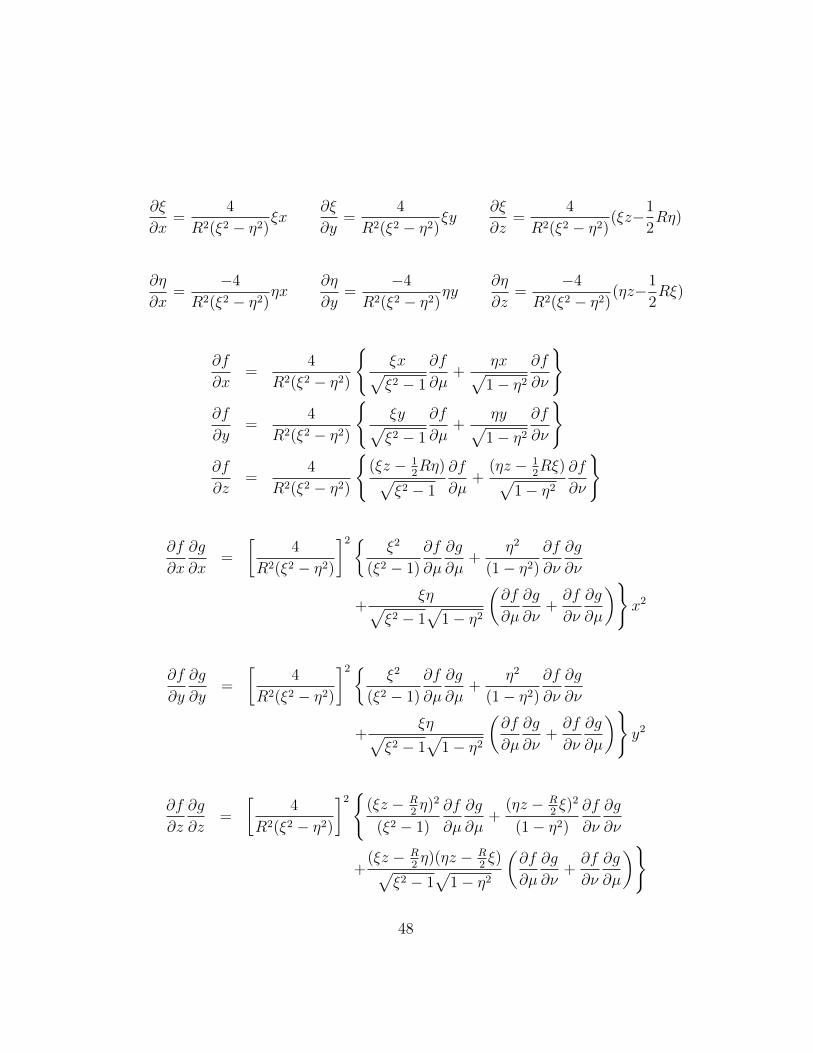
∂ξ

∂x=

4

R2(ξ2 − η2)ξx

∂ξ

∂y=

4

R2(ξ2 − η2)ξy

∂ξ

∂z=

4

R2(ξ2 − η2)(ξz−1

2Rη)

∂η

∂x=

−4

R2(ξ2 − η2)ηx

∂η

∂y=

−4

R2(ξ2 − η2)ηy

∂η

∂z=

−4

R2(ξ2 − η2)(ηz−1

2Rξ)

∂f

∂x=

4

R2(ξ2 − η2)

{ξx√ξ2 − 1

∂f

∂µ+

ηx√1− η2

∂f

∂ν

}∂f

∂y=

4

R2(ξ2 − η2)

{ξy√ξ2 − 1

∂f

∂µ+

ηy√1− η2

∂f

∂ν

}∂f

∂z=

4

R2(ξ2 − η2)

{(ξz − 1

2Rη)√

ξ2 − 1

∂f

∂µ+

(ηz − 12Rξ)√

1− η2

∂f

∂ν

}

∂f

∂x

∂g

∂x=

[4

R2(ξ2 − η2)

]2{ξ2

(ξ2 − 1)

∂f

∂µ

∂g

∂µ+

η2

(1− η2)

∂f

∂ν

∂g

∂ν

+ξη√

ξ2 − 1√

1− η2

(∂f

∂µ

∂g

∂ν+∂f

∂ν

∂g

∂µ

)}x2

∂f

∂y

∂g

∂y=

[4

R2(ξ2 − η2)

]2{ξ2

(ξ2 − 1)

∂f

∂µ

∂g

∂µ+

η2

(1− η2)

∂f

∂ν

∂g

∂ν

+ξη√

ξ2 − 1√

1− η2

(∂f

∂µ

∂g

∂ν+∂f

∂ν

∂g

∂µ

)}y2

∂f

∂z

∂g

∂z=

[4

R2(ξ2 − η2)

]2{

(ξz − R2η)2

(ξ2 − 1)

∂f

∂µ

∂g

∂µ+

(ηz − R2ξ)2

(1− η2)

∂f

∂ν

∂g

∂ν

+(ξz − R

2η)(ηz − R

2ξ)√

ξ2 − 1√

1− η2

(∂f

∂µ

∂g

∂ν+∂f

∂ν

∂g

∂µ

)}

48

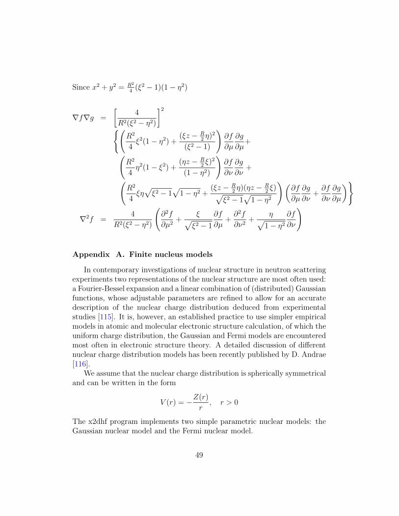
Since x2 + y2 = R2

4(ξ2 − 1)(1− η2)

∇f∇g =

[4

R2(ξ2 − η2)

]2

{(R2

4ξ2(1− η2) +

(ξz − R2η)2

(ξ2 − 1)

)∂f

∂µ

∂g

∂µ+(

R2

4η2(1− ξ2) +

(ηz − R2ξ)2

(1− η2)

)∂f

∂ν

∂g

∂ν+(

R2

4ξη√ξ2 − 1

√1− η2 +

(ξz − R2η)(ηz − R

2ξ)√

ξ2 − 1√

1− η2

)(∂f

∂µ

∂g

∂ν+∂f

∂ν

∂g

∂µ

)}

∇2f =4

R2(ξ2 − η2)

(∂2f

∂µ2+

ξ√ξ2 − 1

∂f

∂µ+∂2f

∂ν2+

η√1− η2

∂f

∂ν

)

Appendix A. Finite nucleus models

In contemporary investigations of nuclear structure in neutron scatteringexperiments two representations of the nuclear structure are most often used:a Fourier-Bessel expansion and a linear combination of (distributed) Gaussianfunctions, whose adjustable parameters are refined to allow for an accuratedescription of the nuclear charge distribution deduced from experimentalstudies [115]. It is, however, an established practice to use simpler empiricalmodels in atomic and molecular electronic structure calculation, of which theuniform charge distribution, the Gaussian and Fermi models are encounteredmost often in electronic structure theory. A detailed discussion of differentnuclear charge distribution models has been recently published by D. Andrae[116].

We assume that the nuclear charge distribution is spherically symmetricaland can be written in the form

V (r) = −Z(r)

r, r > 0

The x2dhf program implements two simple parametric nuclear models: theGaussian nuclear model and the Fermi nuclear model.

49

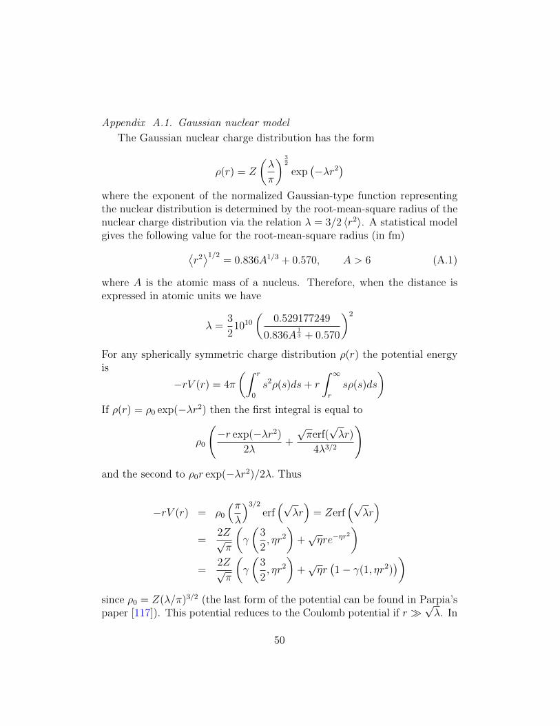
Appendix A.1. Gaussian nuclear model

The Gaussian nuclear charge distribution has the form

ρ(r) = Z

(λ

π

) 32

exp(−λr2

)where the exponent of the normalized Gaussian-type function representingthe nuclear distribution is determined by the root-mean-square radius of thenuclear charge distribution via the relation λ = 3/2 〈r2〉. A statistical modelgives the following value for the root-mean-square radius (in fm)⟨

r2⟩1/2

= 0.836A1/3 + 0.570, A > 6 (A.1)

where A is the atomic mass of a nucleus. Therefore, when the distance isexpressed in atomic units we have

λ =3

21010

(0.529177249

0.836A13 + 0.570

)2

For any spherically symmetric charge distribution ρ(r) the potential energyis

−rV (r) = 4π

(∫ r

0

s2ρ(s)ds+ r

∫ ∞r

sρ(s)ds

)If ρ(r) = ρ0 exp(−λr2) then the first integral is equal to

ρ0

(−r exp(−λr2)

2λ+

√πerf(

√λr)

4λ3/2

)

and the second to ρ0r exp(−λr2)/2λ. Thus

−rV (r) = ρ0

(πλ

)3/2

erf(√

λr)

= Zerf(√

λr)

=2Z√π

(γ

(3

2, ηr2

)+√ηre−ηr

2

)=

2Z√π

(γ

(3

2, ηr2

)+√ηr(1− γ(1, ηr2)

))since ρ0 = Z(λ/π)3/2 (the last form of the potential can be found in Parpia’spaper [117]). This potential reduces to the Coulomb potential if r �

√λ. In

50

case a very tight diatomic system with finite nuclei is considered the Z1Z2/rcontribution to the total energy must be replaced by

Z1Z2

r

1√πγ

(1

2, λ12r

2

)where γ(a, x) is the lower incomplete gamma function

γ(a, x) =

∫ x

0

ta−1e−tdt (A.2)

and 1/λ12 = 1/λ1 + 1/λ2 [117].

Appendix A.2. Fermi nuclear model

The Fermi nuclear model contains more detail concerning the charge dis-tribution than the Gaussian model and has traditionally been employed infitting nuclear scattering data. The Fermi nucleus has the form of a Fermidistribution

ρ(r) =ρ0

1 + e(r−c)/a

where c is the half-density radius since ρ(c) = ρ0/2. The parameter a isrelated to the nuclear skin thickness t through t/a = 4 ln 3. It may be verifiedthat ρ(c − t/2) = 0.9ρ0 and that ρ(c + t/2) = 0.1ρ0. The skin thickness isthus the interval across which the nuclear charge density drops from 0.9ρ0 to0.1ρ0. It is a standard practice to take t = 2.30 fm independent of the atomicmass. The parameter c depends on the atomic mass through Eq. (A.1) andthe following relation ⟨

r2⟩≈ 3

5c2 +

7

5π2a2

The Fermi nuclear potential reads

− rV (r) =Z

N

{6(ac

)3[−S3

(− ca

)+ S3

(r − ca

)]+r

c

[3

2+

1

2π2(ac

)2

− 3(ac

)2

S2

(r − ca

)− 1

2

(rc

)2]}

for r/c < 1 and

− rV (r) =Z

N

{N + 3

(ac

)2[r

cS2

(r − ca

)+ 2

(ac

)S3

(r − ca

)]}51

otherwise; N = 1 + π2(a/c)2 − 6(a/c)3S3(−c/a) and Sk is an infinite seriesdefined as

Sk(r) =∞∑n=1

(−1)nenr

nk

This is the potential for the Fermi charge distribution used in GRASP2package [118] and the x2dhf program follows suit.

Appendix A. Miscelenous formulae

Recursive formula for the Legendre polynomials

Pn+1(z) =1

n+ 1[(2n+ 1)zPn(z)− nPn−1(z)]

Recursive formulae for the associate Legendre polynomials

P qk+1 =

1

k − q + 1

[(2k + 1)zP q

k (z)− (k + q)P qk−1(z)

]P qk =

(−1)qΓ(k + q + 1)(1− z2)q/2

2qΓ(k − q + 1)q!F

(q − k, qk + 1; q + 1;

1− z2

)The program uses the following associate Legrendre polynomials to calculateboundary values from the multipole expansion:

52

P 11 (z) = − 1√

2

√1− z2

P 12 (z) = − 3√

6z√

1− z2

P 13 (z) =

3

2√

12(1− 5z2)

√1− z2

P 14 (z) =

5

2√

20(3z − 7z3)

√1− z2

P 15 (z) =

15

8√

30(−1 + 14z2 − 21z4)

√1− z2

P 16 (z) =

21

8√

42(−5z + 30z3 − 33z5)

√1− z2

P 17 (z) =

7

16√

56(5− 135z2 + 495z4 − 429z6)

√1− z2

P 18 (z) =

9

16√

72(35z − 385z3 + 1001z5 − 715z7)

√1− z2

P 22 (z) =

3√24

(1− z2)

P 23 (z) =

15√120

(z − z3)

P 24 (z) =

15

2√

360(−1 + 8z2 − 7z4)

P 25 (z) =

105

2√

840(−z + 4z3 − 3z5)

P 26 (z) =

108

2√

1680(1− 19z2 + 51z4 − 33z6)

P 27 (z) =

63

8√

3024(15z − 125z3 + 253z5 − 143z7)

P 28 (z) =

315

8√

5040(−1 + 34z2 − 176z4 + 286z6 − 143z8)

53

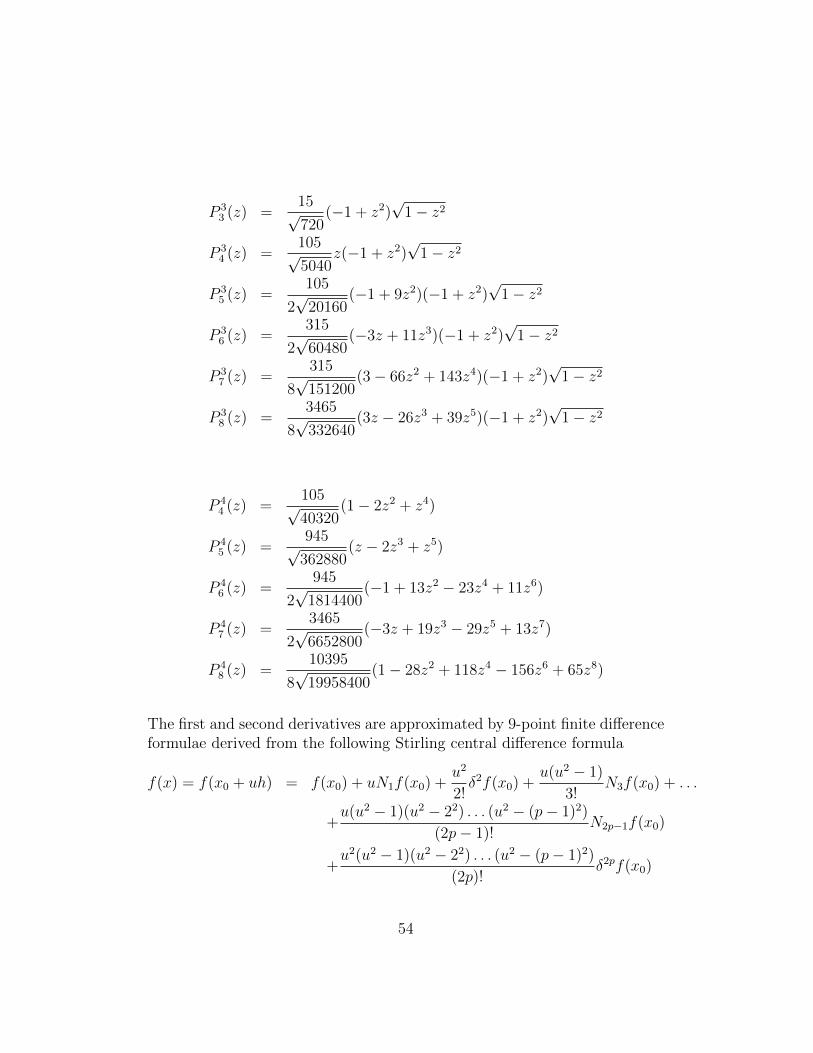
P 33 (z) =

15√720

(−1 + z2)√

1− z2

P 34 (z) =

105√5040

z(−1 + z2)√

1− z2

P 35 (z) =

105

2√

20160(−1 + 9z2)(−1 + z2)

√1− z2

P 36 (z) =

315

2√

60480(−3z + 11z3)(−1 + z2)

√1− z2

P 37 (z) =

315

8√

151200(3− 66z2 + 143z4)(−1 + z2)

√1− z2

P 38 (z) =

3465

8√

332640(3z − 26z3 + 39z5)(−1 + z2)

√1− z2

P 44 (z) =

105√40320

(1− 2z2 + z4)

P 45 (z) =

945√362880

(z − 2z3 + z5)

P 46 (z) =

945

2√

1814400(−1 + 13z2 − 23z4 + 11z6)

P 47 (z) =

3465

2√

6652800(−3z + 19z3 − 29z5 + 13z7)

P 48 (z) =

10395

8√

19958400(1− 28z2 + 118z4 − 156z6 + 65z8)

The first and second derivatives are approximated by 9-point finite differenceformulae derived from the following Stirling central difference formula

f(x) = f(x0 + uh) = f(x0) + uN1f(x0) +u2

2!δ2f(x0) +

u(u2 − 1)

3!N3f(x0) + . . .

+u(u2 − 1)(u2 − 22) . . . (u2 − (p− 1)2)

(2p− 1)!N2p−1f(x0)

+u2(u2 − 1)(u2 − 22) . . . (u2 − (p− 1)2)

(2p)!δ2pf(x0)

54

where

δf(x0) = f(x0 + h/2)− f(x0 − h/2)

δkf(x0) = δ(δk−1f(x0)

)Nkf(x0) =

1

2

(δkf(x0 + h/2) + δkf(x0 − h/2)

)References

[1] F. Jensen, Introduction to computational chemistry, Wiley, New York,1999.

[2] E. L. Albasiny, J. R. A. Cooper, Mol. Phys. 4 (1961) 353–358.

[3] E. L. Albasiny, J. R. A. Cooper, Proc. Phys. Soc. 82 (1963) 289–303.

[4] E. L. Albasiny, J. R. A. Cooper, Proc. Phys. Soc. 85 (1965) 1133–1142.

[5] E. L. Albasiny, J. R. A. Cooper, Proc. Phys. Soc. 88 (1966) 315–323.

[6] J. A. Keefer, J. K. Su Fu, R. L. Belford, J. Chem. Phys. 50 (1969)160–173.

[7] A. D. Becke, R. M. Dickson, J. Chem. Phys. 89 (1988) 2993–2997.

[8] A. D. Becke, R. M. Dickson, J. Chem. Phys. 92 (1990) 3610–3612.

[9] R. M. Dickson, A. D. Becke, J. Chem. Phys. 99 (1993) 3898–3905.

[10] T. Shiozaki, S. Hirata, Phys. Rev. A 76 (2007) 040503.

[11] E. A. McCullough Jr., Chem. Phys. Lett. 24 (1974) 55–58.

[12] E. A. McCullough Jr., Comput. Phys. Rep. 4 (1986) 265–312.

[13] A. D. Becke, J. Chem. Phys. 76 (1982) 6037–6045.

[14] A. D. Becke, J. Chem. Phys. 78 (1983) 4787–4788.

[15] A. D. Becke, Int. J. Quantum Chem. 27 (1985) 585.

[16] A. D. Becke, Phys. Rev. A 33 (1986) 2786.

55

[17] A. N. Artemyev, E. V. Ludena, V. Karasiev, A. J. Hernandez, J. Com-put. Chem. 25 (2003) 368–374.

[18] D. Heinemann, D. Kolb, B. Fricke, Chem. Phys. Lett. 137 (1987) 180–182.

[19] D. Heinemann, B. Fricke, D. Kolb, Phys. Rev. A 38 (1988) 4994–5001.

[20] D. Heinemann, A. Rosen, B. Fricke, Physica Scripta 42 (1990) 692–696.

[21] O. Beck, D. Heinemann, D. Kolb, arXiv:physics/0307108v1[physics.comp-ph] (????).

[22] S. Hackel, D. Heinemann, D. Kolb, B. Fricke, Chem. Phys. Lett. 206(1993) 91–95.

[23] L. Yang, D. Heinemann, D. Kolb, Chem. Phys. Lett. 178 (1991) 213.

[24] L. Yang, D. Heinemann, D. Kolb, Chem. Phys. Lett. 192 (1992) 499.

[25] C. Dusterhoft, L. Yang, D. Heinemann, D. Kolb, Chem. Phys. Lett.229 (1994) 667–670.

[26] D. Sundholm, Comput. Phys. Commun. 49 (1988) 409.

[27] D. Sundholm, J. Olsen, P. Malmqvist, B. O. Roos, in: M. Defranceschi,J. Delhalle (Eds.), Numerical determination of the electronic structureof atoms diatomic and polyatomic molecules, volume 271 of NATO ASISeries, Series C: Mathematical and Physical Sciences, Kluwer Aca-demic Publishers, Dordrecht, 1989, pp. 329–334.

[28] D. Sundholm, J. Olsen, Proc. 13th. IMACS World Congress on Com-putation and Applied Mathematics, Criterion, Dublin, 1991, p. 861.

[29] J. C. Morrison, T. Wolf, B. Bialecki, G. F. Weather, L. Larson, Mol.Phys. 98 (2000) 1175–1184.

[30] J. C. Morrison, S. Boyd, L. Marsano, B. Bialecki, T. Ericsson, J. P.Santos, Commun. Comput. Phys. 5 (2009) 959–985.

[31] L. Laaksonen, P. Pyykko, D. Sundholm, Comput. Phys. Rep. 4 (1986)313–344.

56

[32] K. Davstad, J. Chem. Phys. 99 (1992) 33–38.

[33] T. Beck, Rev. Mod. Phys. 72 (2000) 1041–1080.

[34] T. A. Arias, Rev. Mod. Phys. 71 (1999) 267.

[35] J. Kobus, Chem. Phys. Lett. 202 (1993) 7–12.

[36] J. Kobus, Comput. Phys. Commun. 78 (1994) 247–255.

[37] J. Kobus, Adv. Quantum Chem. 28 (1997) 1–14.

[38] J. Kobus, L. Laaksonen, D. Sundholm, Comput. Phys. Commun. 98(1996) 346–358.

[39] J. Kobus, in: S. Wilson, P. F. Bernath, R. McWeeny (Eds.), Hand-book of Molecular Physics and Quantum Chemistry, volume 2, chap.9, Wiley, Chichester, 2003.

[40] D. Moncrieff, S. Wilson, Chem. Phys. Lett. 209 (1993) 423–426.

[41] D. Moncrieff, S. Wilson, J. Phys. B: At. Mol. Opt. Phys. 26 (1993)1605–1616.

[42] J. Kobus, D. Moncrieff, S. Wilson, J. Phys. B: At. Mol. Opt. Phys. 27(1994) 2867–2875.

[43] J. Kobus, D. Moncrieff, S. Wilson, J. Phys. B: At. Mol. Opt. Phys. 27(1994) 5139–5147.

[44] J. Kobus, D. Moncrieff, S. Wilson, Mol. Phys. 86 (1995) 1315–1330.

[45] D. Moncrieff, J. Kobus, S. Wilson, J. Phys. B: At. Mol. Opt. Phys. 28(1995) 4555–4557.

[46] D. Moncrieff, S. Wilson, J. Phys. B: At. Mol. Opt. Phys. 29 (1996)2425–2451.

[47] D. Moncrieff, J. Kobus, S. Wilson, Mol. Phys. 93 (1998) 713–725.

[48] J. Kobus, D. Moncrieff, S. Wilson, Mol. Phys. 96 (1999) 1559–1567.

[49] J. Kobus, D. Moncrieff, S. Wilson, Phys. Rev. A 62 (2000) 062503/1–9.

57

[50] J. Kobus, D. Moncrieff, S. Wilson, Mol. Phys. 98 (2000) 401–408.

[51] J. Kobus, D. Moncrieff, S. Wilson, Mol. Phys. 100 (2002) 499–508.

[52] J. Kobus, D. Moncrieff, S. Wilson, J. Phys. B: At. Mol. Opt. Phys. 34(2001) 5127–5143.

[53] J. Kobus, D. Moncrieff, S. Wilson, J. Phys. B: At. Mol. Opt. Phys. 37(2004) 571–585.

[54] J. Kobus, D. Moncrieff, S. Wilson, J. Phys. B: At. Mol. Opt. Phys. 40(2007) 877–896.

[55] J. Kobus, Comp. Lett. 3 (2007) 71–113.

[56] J. Kobus, Special Volume of the American Institute of Physics Confer-ence Proceedings.

[57] A. Halkier, W. Klopper, T. Halgaker, P. Jørgensen, J. Chem. Phys.111 (1999) 4424–4430.

[58] A. Halkier, T. Helgaker, P. Jørgensen, W. Klopper, J. Olsen, Chem.Phys. Lett. 302 (1999) 437–446.

[59] K. Aa. Christensen, F. Jensen, Chem. Phys. Lett. 317 (2000) 400–403.

[60] F. Jensen, J. Chem. Phys. 110 (1999) 6601–6605.

[61] F. Jensen, Theor. Chem. Acc. 104 (2000) 484–490.

[62] F. Jensen, J. Chem. Phys. 115 (2001) 9113.

[63] F. Jensen, J. Chem. Phys. 116 (2002) 7372–7379.

[64] F. Jensen, J. Chem. Phys. 117 (2002) 9234–9240.

[65] S. Shahbazian1, M. Zahedi, Theor. Chem. Acc. 113 (2005) 152–160.

[66] T. G. Williams, N. J. DeYonker, A. K. Wilson, The Journal of ChemicalPhysics 128 (2008) 044101.

[67] N. B. Balabanov, K. A. Peterson, J. Chem. Phys. 123 (2005) 064107.

58

[68] A. Helgakier, W. Klopper, H. Koch, J. Noga, J. Chem. Phys. 106 (1997)9639.

[69] S. Zhong, E. C. Barnes, G. A. Petersson, The Journal of ChemicalPhysics 129 (2008) 184116.

[70] F. Jensen, Theor. Chem. Acc. 113 (2005) 187–190.

[71] S. C. A. Halkier, Chem. Phys. Lett. 346 (2001) 329–333.

[72] F. Paw lowski, P. Jørgensen, C. Hattig, Chem. Phys. Lett. 391 (2004)27–32.

[73] J. Styszynski, Chem. Phys. Lett. 317 (2000) 351–359.

[74] J. Styszynski, J. Kobus, Chem. Phys. Lett. 369 (2003) 441–448.

[75] E. Matito, J. Kobus, , J. Styszyski, Chem. Phys. 321 (2005) 277–284.

[76] A. K. Roy, A. J. Thakkar, Chem. Phys. Lett. 362 (2002) 428–434.

[77] J. F. Ziegler, J. P. Biersack, U. Littmark, The Stopping and Range ofIons in Solids, Pergamon, New York, 1985.

[78] K. Nordlund, N. Runeberg, D. Sundholm, Nucl. Instrum. Meth. B 132(1997) 45–54.

[79] J. Pruneda, E. Artacho, PHYSICAL REVIEW B 70 (2004).

[80] V. Kuzmin, Nuclear Instruments and Methods in Physics ResearchSection B: Beam Interactions with Materials and Atoms 249 (2006)113–17.

[81] V. Kuzmin, Surface and Coatings Technology 201 (2007) 8388–8392.

[82] C. B. Madsen, L. B. Madsen, Phys. Rev. A 74 (2006) 023403.

[83] S. Liu, V. K. R. Lopez-Boada, F. De Proft, Int. J. Quantum Chem. 69(1998) 513–522.

[84] E. V. Ludena, V. V. K. R. Lopez-Boada, E. Valderrama, J. Maldonado,J. Comp. Chem. 20 (1999) 155–183.

59

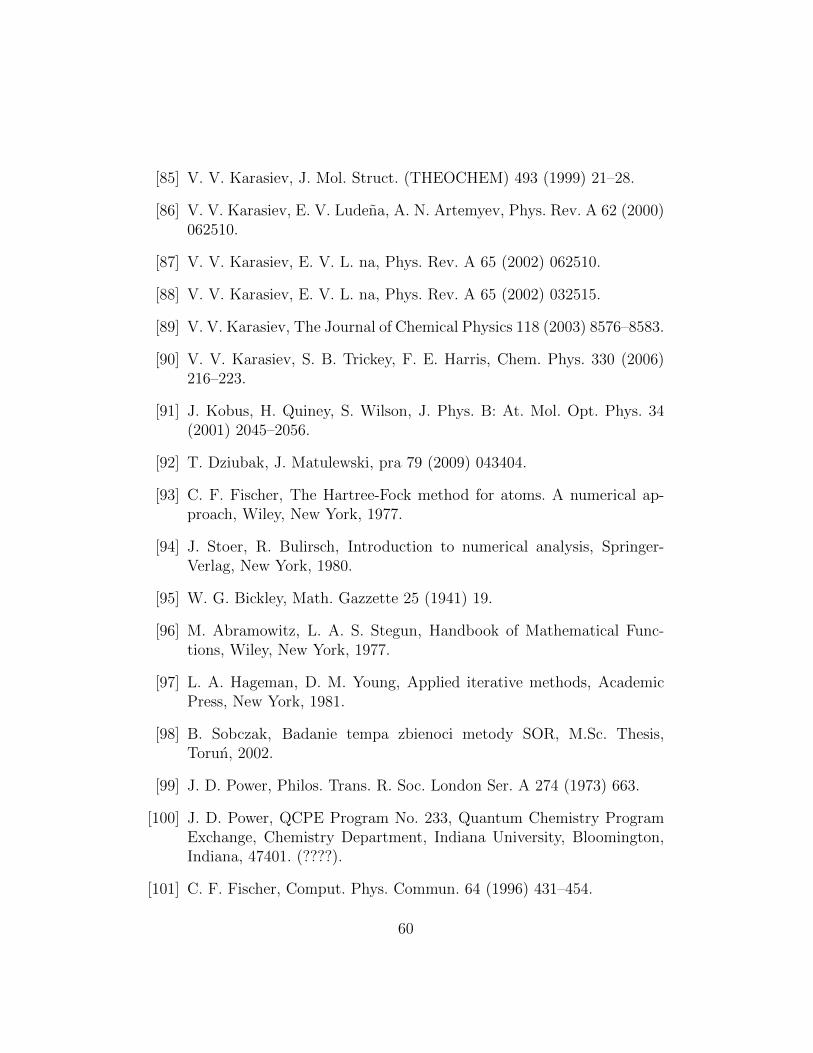
[85] V. V. Karasiev, J. Mol. Struct. (THEOCHEM) 493 (1999) 21–28.

[86] V. V. Karasiev, E. V. Ludena, A. N. Artemyev, Phys. Rev. A 62 (2000)062510.

[87] V. V. Karasiev, E. V. L. na, Phys. Rev. A 65 (2002) 062510.

[88] V. V. Karasiev, E. V. L. na, Phys. Rev. A 65 (2002) 032515.

[89] V. V. Karasiev, The Journal of Chemical Physics 118 (2003) 8576–8583.

[90] V. V. Karasiev, S. B. Trickey, F. E. Harris, Chem. Phys. 330 (2006)216–223.

[91] J. Kobus, H. Quiney, S. Wilson, J. Phys. B: At. Mol. Opt. Phys. 34(2001) 2045–2056.

[92] T. Dziubak, J. Matulewski, pra 79 (2009) 043404.

[93] C. F. Fischer, The Hartree-Fock method for atoms. A numerical ap-proach, Wiley, New York, 1977.

[94] J. Stoer, R. Bulirsch, Introduction to numerical analysis, Springer-Verlag, New York, 1980.

[95] W. G. Bickley, Math. Gazzette 25 (1941) 19.

[96] M. Abramowitz, L. A. S. Stegun, Handbook of Mathematical Func-tions, Wiley, New York, 1977.

[97] L. A. Hageman, D. M. Young, Applied iterative methods, AcademicPress, New York, 1981.

[98] B. Sobczak, Badanie tempa zbienoci metody SOR, M.Sc. Thesis,Torun, 2002.

[99] J. D. Power, Philos. Trans. R. Soc. London Ser. A 274 (1973) 663.

[100] J. D. Power, QCPE Program No. 233, Quantum Chemistry ProgramExchange, Chemistry Department, Indiana University, Bloomington,Indiana, 47401. (????).

[101] C. F. Fischer, Comput. Phys. Commun. 64 (1996) 431–454.

60

[102] L. S. Blackford, J. Demmel, J. Dongarra, I. Duff, S. Hammarling,G. Henry, M. Heroux, L. Kaufman, A. Lumsdaine, A. Petitet, R. Pozo,K. Remington, R. C. Whaley, ACM Trans. Math. Soft. 28-2 (2002)135–151.

[103] A. D. Becke, Phys. Rev. A 88 (1988) 3098–3100.

[104] C. Lee, W. Yang, R. Parr, Phys. Rev. B 37 (1988) 785–789.

[105] S. H. Vosko, L. Wilk, M. Nusair, Can. J. Phys. 58 (1980) 1200.

[106] K. Schwarz, Phys. Rev. B 5 (1972) 2466–2468.

[107] A. E. S. Green, D. L. Sellin, A. S. Zachor, Phys. Rev. 184 (1969) 1–9.

[108] A. D. Buckingham, Adv. Chem. Phys. 12 (1967) 107.

[109] A. D. McLean, M. Yoshimine, J. Chem. Phys. 47 (1967) 1927.

[110] G. Maroulis, J. Chem. Phys. 118 (2003) 2673–2687.

[111] A. H. WAPSTRA, G. AUDI, Nucl. Phys. A 432 (1983) 1–54.

[112] G. AUDI, A. H. WAPSTRA, Nucl. Phys. A 565 (1993) 1–65.

[113] J. P. Perdew, W. Yue, Phys. Rev. B 33 (1986) 8800–8802.

[114] J. P. Perdew, J. A. Chevary, S. H. Vosko, K. A. Jackson, M. R. Peder-son, C. Fiolhais, Phys. Rev. B 46 (1992) 6671.

[115] H. de Vries, C. W. de Jager, C. de Vries, At. Data Nucl. Data Tables36 (1987) 495.

[116] D. Andrae, Phys. Rep. 336 (2000) 414–525.

[117] F. A. Parpia, J. Phys. B: At. Mol. Opt. Phys. 30 (1997) 3983–4001.

[118] F. A. Parpia, C. Froese Fischer, I. P. Grant, Comput. Phys. Commun.94 (1996) 249–271.

[119] B. G. Johnson, P. M. W. Gill, J. A. Pople, J. Chem. Phys. 98 (1993)5612–5626.

61

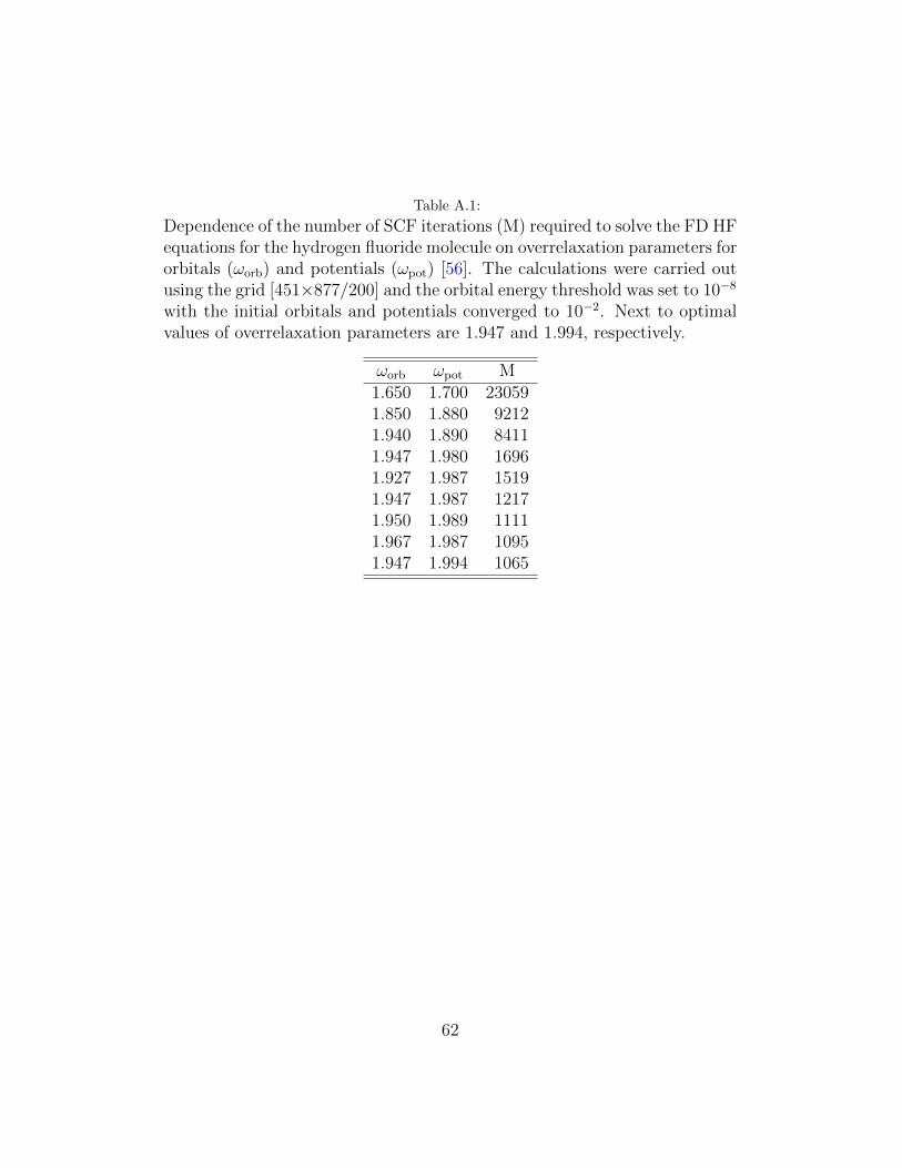
Table A.1:

Dependence of the number of SCF iterations (M) required to solve the FD HFequations for the hydrogen fluoride molecule on overrelaxation parameters fororbitals (ωorb) and potentials (ωpot) [56]. The calculations were carried outusing the grid [451×877/200] and the orbital energy threshold was set to 10−8

with the initial orbitals and potentials converged to 10−2. Next to optimalvalues of overrelaxation parameters are 1.947 and 1.994, respectively.

ωorb ωpot M1.650 1.700 230591.850 1.880 92121.940 1.890 84111.947 1.980 16961.927 1.987 15191.947 1.987 12171.950 1.989 11111.967 1.987 10951.947 1.994 1065

62

Table A.2: Dependence of the number of SOR iterations (total SOR) and the time (inseconds) required to solve the FD HF equations on the number of SOR iterations used torelax orbitals and potentials in a single SCF iteration (SOR/SCF). The calculations werecarried out using as initial orbitals and potentials functions converged to within 10−4 (inorbital energy) and were stopped when the largest differences in orbital energies betweentwo successive SCF iteration were less than 10−10.

SOR/SCF 5 10 15 20 30 40 50Be [169× 217/35]total SOR 1520 1670 1785 1840 1860 1960 2000time 29.5 27.6 26.1 25.2 25.2 21.5 24.1BO [169× 223/40]total SOR 2730 2990 3285 3700 4260 4600 19450time 310.1 269.4 276.2 295.9 312.6 344.1 1468.2BO [265× 361/40]total SOR 4555 4870 4935 4780 5160 6120 6750time 1269.9 1080.5 1009.6 922.7 938.3 1073.9 1257.0

63

Table A.3: Dependence of the hydrogen ground state kinetic, nuclear and the totalenergy on discretization errors (r∞ = 25 bohr) when the exact 1 σ function is used.Discretization errors due to the kinetic energy operator are proportional to h8 where his equal to the step size in ν/µ variables (hν ≈ hµ). Integration errors are of the sameorder of magnitude. |1−〈I〉 | denotes the error of 1σ normalization constant and 1

2 −〈T 〉,−1− 〈Vn〉 and − 1

2 − 〈T + Vn〉 denote the absolute errors of the kinetic, nuclear and totalenergy, respectively.

Nν ×Nµ h8 |1− 〈I〉 | 12− 〈T 〉 −1− 〈Vn〉 −1

2− 〈T + Vn〉

7× 7 6.4× 10−2 1.1× 10−1 −2.8× 10−2 2.1× 10−2 −7.0× 10−3

13× 19 2.1× 10−5 1.9× 10−5 1.7× 10−4 −1.7× 10−4 1.7× 10−6

25× 31 1.5× 10−7 3.6× 10−6 −2.6× 10−6 2.7× 10−6 1.1× 10−9

37× 49 3.9× 10−9 2.3× 10−8 −3.3× 10−8 3.3× 10−8 4.0× 10−11

55× 73 1.5× 10−10 1.4× 10−10 −4.8× 10−10 5.0× 10−10 1.6× 10−12

103× 139 8.5× 10−13 7.4× 10−13 −2.7× 10−12 2.8× 10−12 5.1× 10−14

64

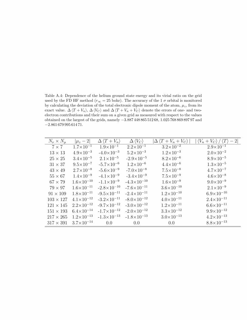
Table A.4: Dependence of the helium ground state energy and its virial ratio on the gridused by the FD HF method (r∞ = 25 bohr). The accuracy of the 1 σ orbital is monitoredby calculating the deviation of the total electronic dipole moment of the atom, µz, from itsexact value. ∆ 〈T + Vn〉, ∆ 〈VC〉 and ∆ 〈T + Vn + VC〉 denote the errors of one- and two-electron contributions and their sum on a given grid as measured with respect to the valuesobtained on the largest of the grids, namely −3.887 448 865 512 68, 1.025 768 869 897 97 and−2.861 679 995 614 71.

Nν ×Nµ |µz − 2| ∆ 〈T + Vn〉 ∆ 〈VC〉 |∆ 〈T + Vn + VC〉 | | 〈Vn + VC〉 / 〈T 〉 − 2|7× 7 1.7×10−1 1.9×10−1 2.2×10−1 3.2×10−2 2.9×10−1

13× 13 4.9×10−3 -4.0×10−3 5.2×10−3 1.2×10−3 2.0×10−2

25× 25 3.4×10−5 2.1×10−5 -2.9×10−5 8.2×10−6 8.9×10−5

31× 37 9.5×10−7 -5.7×10−6 1.2×10−6 4.4×10−6 1.3×10−5

43× 49 2.7×10−8 -5.6×10−9 -7.0×10−8 7.5×10−8 4.7×10−7

55× 67 1.4×10−9 -4.1×10−9 -3.4×10−9 7.5×10−9 4.6×10−8

67× 79 1.6×10−10 -1.1×10−9 -4.3×10−10 1.6×10−9 9.0×10−9

79× 97 1.6×10−11 -2.8×10−10 -7.6×10−11 3.6×10−10 2.1×10−9

91× 109 1.8×10−11 -9.5×10−11 -2.4×10−11 1.2×10−10 6.9×10−10

103× 127 4.1×10−12 -3.2×10−11 -8.0×10−12 4.0×10−11 2.4×10−11

121× 145 2.2×10−12 -9.7×10−12 -3.0×10−12 1.2×10−11 6.6×10−11

151× 193 6.4×10−14 -1.7×10−12 -2.0×10−12 3.3×10−12 9.9×10−12

217× 265 1.2×10−13 -1.3×10−13 -1.8×10−13 3.0×10−13 4.2×10−13

317× 391 3.7×10−14 0.0 0.0 0.0 8.8×10−13

Table A.5: Comparison of FD energies (in a.u.) for the GaF+39 one-electron system(R=3.353 bohr, [649×1129/200]) with the exact values from Power’s program (OEDM)[56]. Orbitals are labeled with nlm triplet where n, l and m are principal, orbital andmagnetic quantum numbers, respectively.

nlm OEDM FD100 −483.184 164 997 5 −483.184 164 997 9210 −122.888 205 876 7 −122.888 205 876 8200 −122.733 220 197 1 −122.733 220 197 1320 −56.325 432 982 08 −56.325 432 982 09310 −56.064 747 360 03 −56.064 747 360 04300 −55.857 809 071 15 −55.857 809 071 16430 −49.748 077 736 59 −49.748 077 736 62540 −33.278 686 476 70 −33.278 686 476 95420 −32.852 093 071 00 −32.852 093 071 00

211 −122.807 726 783 2 −122.807 726 783 2321 −56.186 870 411 89 −56.186 870 411 65311 −55.955 787 708 24 −55.955 787 708 00431 −33.044 405 068 15 −33.044 405 068 14

322 −56.064 605 666 57 −56.064 605 666 58432 −32.851 020 550 42 −32.851 020 550 43422 −32.549 061 245 47 −32.549 061 245 47

433 −32.688 193 618 11 −32.688 193 618 11543 −22.037 772 085 85 −22.037 772 085 85533 −21.676 770 733 19 −21.676 770 733 15

66

Table A.6: Camparison of orbital (Eorb) and total (Etot) energies of the Ca atom (in a.u.)obtained by the one-dimensional (1D) and two-dimensional (2D) FD HF method (cor-responding orbital labels are given in parentheses) [56]. Calculations were performedusing the one- and two-dimensional grids defined as ρ0=-18, h=0.0156, N=2500 and[451×859/200], respectively.

1D Eorb/Etot 2D Eorb/Etot

−0.195 529 692 462 (4s) −0.195 529 692 550 (6σ)−1.340 706 956 90 (3p) −1.340 706 956 98 (5σ/2π)−2.245 376 006 03 (3s) −2.245 376 006 11 (4σ)−13.629 269 206 5 (2p) −13.629 269 206 6 (3σ/1π)−16.822 744 273 6 (2s) −16.822 744 273 7 (2σ)−149.363 725 893 (1s) −149.363 725 893 (1σ)−676.758 185 924 −676.758 185 926

Table A.7: Camparison of total HF energies calculated by the finite difference (EFD) andthe multigrid finite element (EFE) methods [56]. The FE results correspond to extrap-olated values from a series of calculations performed on grids of increasing density [21].[Nν×Nµ/r∞] denotes the FD grid. The FD results for the Be and LiH systems were takenfrom [55].

System [Nν×Nµ/r∞] EFD EFE

LiH (R=3.015 au) [259×433/150] −7.987 352 237 23 −7.987 352 237 228Be (R=2.386 au) [349×643/200] −14.573 023 168 3 −14.573 023 168 305BH (R=2.336 au) [349×643/200] −25.131 598 702 3 −25.131 598 702 31N2 (R=2.068 au) [445×841/200] −108.993 825 634 −108.993 825 634 82

67

Table A.8: Total energies of the He, Be and Ne atoms calculated using various combi-nations of local exchange (LDA and B88) and correlation potentials (LYP and VWN).Algebraic results of Johnson, Gill and Pople [119] (denoted FB) are compared with thecorresponding values obtained within the finite difference method (FD).

system HF LDA LDA+VWN LDA+LYP B88 B88+VWN B88+LYPHeFB 2.8552 2.7146 2.8267 2.7582 2.8540 2.9671 2.8978FD 2.861680 2.723640 2.833886 2.767056 2.861725 2.972987 2.905317BeFB 14.5669 14.2164 14.4420 14.3119 14.5606 14.78691 14.6563FD 14.573026 14.223291 14.445390 14.318062 14.564197 14.787469 14.659353NeFB 128.4744 127.3950 128.1419 127.7777 128.4964 129.2442 128.6262FD 128.547098 127.49074 128.228894 127.873286 128.587350 129.326586 128.970274

Table A.9: Total (absolute) energies of the Be and Ne atoms calculated using LDA, B88and SCα-LDA potentials within the finite difference method as modified by Karasiev andLudenia (FD-KL) [87] (note a typo in the LDA energy for the Be atom in Table II of theirpaper) and the present author (FD).

system HF LDA B88 SCα-LDABeFD-KL 14.2233 14.5664 14.5707FD 14.573026 14.223291 14.564244 14.570693NeFD-KL 128.5471 127.4907 128.5901 128.5322FD 128.547098 127.490741 128.587350 128.533177

68

Table A.10: Exchange (absolute) energies of the Be and Ne atoms calculated using LDA,B88 and SCα-LDA potentials within the finite difference method as modified by Karasievand Ludenia (FD-KL) [87] and the present author (FD).

system HF LDA B88 SCα-LDABeFD-KL 2.667 2.278 2.652 2.663FD 2.666914 2.277843 2.684667 2.663346NeFD-KL 12.108 10.937 12.086 12.065FD 12.108351 10.937090 12.139002 12.065332

69

Table A.11: Electrical properties of the FH molecule calculated by means of the finitefield on [451× 877/200] grid using the data from the upper part of the table. µz, αzz, etc.denote the z-components of the total dipole moment, polarizability, etc. with respect tothe centre of mass while ET , µez and Θe

zz denote the total energy and electrical dipole andquadrupole moments for a give field strength. Entries with ∆ show the properties whenthe raw data are modified by a relative error 10−12.

field strength ET µez Θezz

-0.0002 -100.070 823 358 990 -0.104 967 386 574 450 -1.044 975 755 481 64-0.0001 -100.070 812 891 021 -0.104 391 834 078 358 -1.044 577 910 264 440.0 -100.070 802 480 605 -0.103 816 366 336 909 -1.044 180 598 585 64

+0.0001 -100.070 792 127 745 -0.103 240 983 076 439 -1.043 783 820 062 32+0.0002 -100.070 781 832 421 -0.102 665 684 024 677 -1.043 387 574 315 97µz 0.755 983 631 461 119 0.756 075 857 950 02µz + ∆ 0.755 982 964 308 859 0.756 075 857 950 78

αzz 5.755 839 419 900 136 5.754 254 554 649 43αzz + ∆ 5.769 182 465 087 396 5.754 254 555 345 37

βzzz -8.085 976 332 949 940 -8.448 086 128 802 03βzzz + ∆ 91.986 862 571 502 570 -8.448 100 082 570 72

γzzzz 272.967 398 684 543γzzzz + ∆ 272.862 996 086 865

Az,zz 3.970 450 376 067 36Az,zz + ∆ 3.970 450 383 032 16

Bzz,zz -53.315 512 212 511 4Bzz,zz + ∆ -53.315 651 508 493 5

70

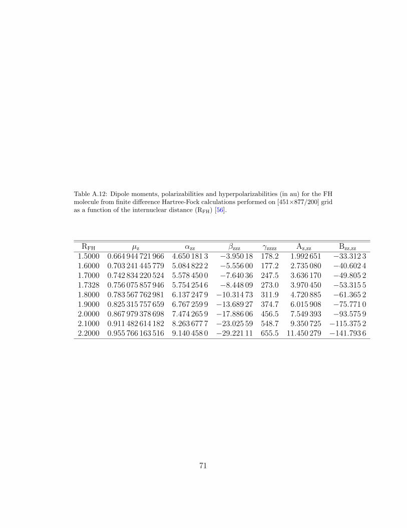
Table A.12: Dipole moments, polarizabilities and hyperpolarizabilities (in au) for the FHmolecule from finite difference Hartree-Fock calculations performed on [451×877/200] gridas a function of the internuclear distance (RFH) [56].

RFH µz αzz βzzz γzzzz Az,zz Bzz,zz

1.5000 0.664 944 721 966 4.650 181 3 −3.950 18 178.2 1.992 651 −33.312 31.6000 0.703 241 445 779 5.084 822 2 −5.556 00 177.2 2.735 080 −40.602 41.7000 0.742 834 220 524 5.578 450 0 −7.640 36 247.5 3.636 170 −49.805 21.7328 0.756 075 857 946 5.754 254 6 −8.448 09 273.0 3.970 450 −53.315 51.8000 0.783 567 762 981 6.137 247 9 −10.314 73 311.9 4.720 885 −61.365 21.9000 0.825 315 757 659 6.767 259 9 −13.689 27 374.7 6.015 908 −75.771 02.0000 0.867 979 378 698 7.474 265 9 −17.886 06 456.5 7.549 393 −93.575 92.1000 0.911 482 614 182 8.263 677 7 −23.025 59 548.7 9.350 725 −115.375 22.2000 0.955 766 163 516 9.140 458 0 −29.221 11 655.5 11.450 279 −141.793 6

71

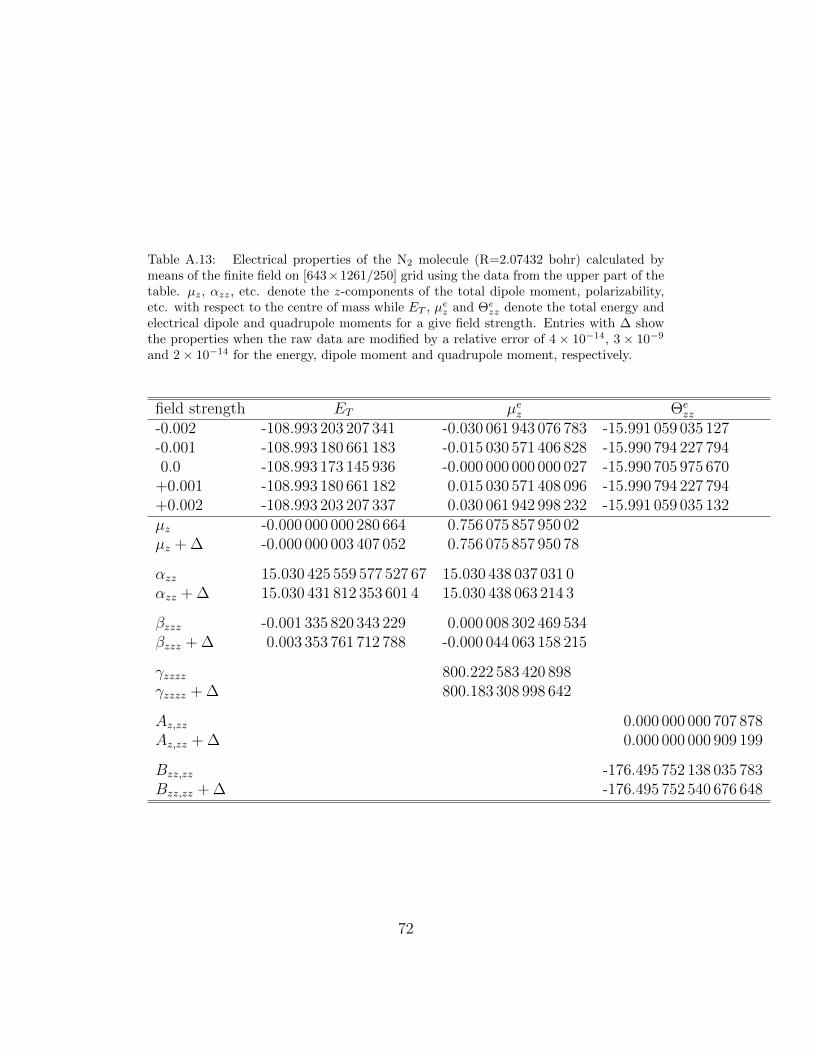
Table A.13: Electrical properties of the N2 molecule (R=2.07432 bohr) calculated bymeans of the finite field on [643×1261/250] grid using the data from the upper part of thetable. µz, αzz, etc. denote the z-components of the total dipole moment, polarizability,etc. with respect to the centre of mass while ET , µez and Θe

zz denote the total energy andelectrical dipole and quadrupole moments for a give field strength. Entries with ∆ showthe properties when the raw data are modified by a relative error of 4 × 10−14, 3 × 10−9

and 2× 10−14 for the energy, dipole moment and quadrupole moment, respectively.

field strength ET µez Θezz

-0.002 -108.993 203 207 341 -0.030 061 943 076 783 -15.991 059 035 127-0.001 -108.993 180 661 183 -0.015 030 571 406 828 -15.990 794 227 7940.0 -108.993 173 145 936 -0.000 000 000 000 027 -15.990 705 975 670

+0.001 -108.993 180 661 182 0.015 030 571 408 096 -15.990 794 227 794+0.002 -108.993 203 207 337 0.030 061 942 998 232 -15.991 059 035 132µz -0.000 000 000 280 664 0.756 075 857 950 02µz + ∆ -0.000 000 003 407 052 0.756 075 857 950 78

αzz 15.030 425 559 577 527 67 15.030 438 037 031 0αzz + ∆ 15.030 431 812 353 601 4 15.030 438 063 214 3

βzzz -0.001 335 820 343 229 0.000 008 302 469 534βzzz + ∆ 0.003 353 761 712 788 -0.000 044 063 158 215

γzzzz 800.222 583 420 898γzzzz + ∆ 800.183 308 998 642

Az,zz 0.000 000 000 707 878Az,zz + ∆ 0.000 000 000 909 199

Bzz,zz -176.495 752 138 035 783Bzz,zz + ∆ -176.495 752 540 676 648

72

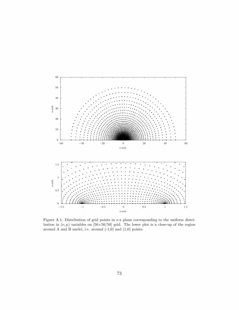
0

10

20

30

40

50

60

x-axis

−60 −40 −20 0 20 40 60

z-axis

0

0.5

1

1.5

x-axis

−1.5 −1 −0.5 0 0.5 1 1.5

z-axis

Figure A.1: Distribution of grid points in z-x plane corresponding to the uniform distri-bution in (ν, µ) variables on [50×50/50] grid. The lower plot is a close-up of the regionaround A and B nuclei, i.e. around (-1,0) and (1,0) points.

73

10−16

10−14

10−12

10−10

10−8

10−6

10−4

10−2

100

Orbital

energy

differen

ces(H

artree)

0 2 · 103 4 · 103 6 · 103 8 · 103 1 · 104 1.2 · 104

SCF iterations

1 σ

10−14

10−12

10−10

10−8

10−6

10−4

10−2

100

Orbital

energy

differen

ces(H

artree)

0 2 · 103 4 · 103 6 · 103 8 · 103 1 · 104 1.2 · 104

SCF iterations

2 σ

Figure A.2: Convergence patterns of 1 σ and 2 σ FH orbitals discretized on [451×877/200]grid for suboptimal overrelaxation parameters: ωorb = 1.65, ωpot = 1.68.

74

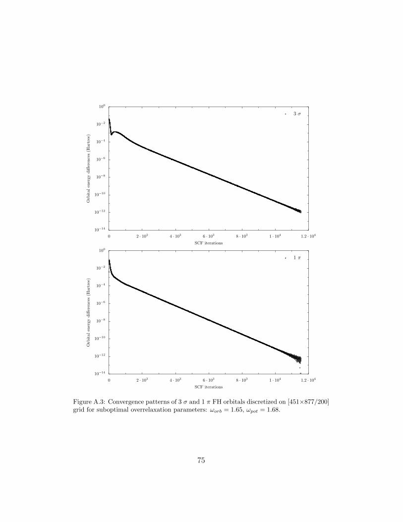
10−14

10−12

10−10

10−8

10−6

10−4

10−2

100

Orbital

energy

differen

ces(H

artree)

0 2 · 103 4 · 103 6 · 103 8 · 103 1 · 104 1.2 · 104

SCF iterations

3 σ

10−14

10−12

10−10

10−8

10−6

10−4

10−2

100

Orbital

energy

differen

ces(H

artree)

0 2 · 103 4 · 103 6 · 103 8 · 103 1 · 104 1.2 · 104

SCF iterations

1 π

Figure A.3: Convergence patterns of 3 σ and 1 π FH orbitals discretized on [451×877/200]grid for suboptimal overrelaxation parameters: ωorb = 1.65, ωpot = 1.68.

75

10−14

10−12

10−10

10−8

10−6

10−4

10−2

100

Orbital

energy

differen

ces(H

artree)

0 500 1000 1500 2000

SCF iterations

1 σ

10−14

10−12

10−10

10−8

10−6

10−4

10−2

100

Orbitalen

ergydifferen

ces(H

artree)

0 500 1000 1500 2000

SCF iterations

2 σ

Figure A.4: Convergence patterns of 1 σ and 2 σ FH orbitals discretized on [451×877/200]grid for near optimal overrelaxation parameters: ωorb = 1.950, ωpot = 1.989.

76

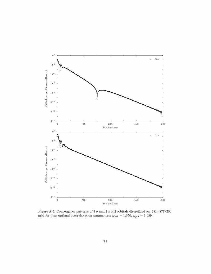
10−14

10−12

10−10

10−8

10−6

10−4

10−2

100

Orbital

energy

differen

ces(H

artree)

0 500 1000 1500 2000

SCF iterations

3 σ

10−14

10−12

10−10

10−8

10−6

10−4

10−2

100

Orbitalen

ergydifferen

ces(H

artree)

0 500 1000 1500 2000

SCF iterations

1 π

Figure A.5: Convergence patterns of 3 σ and 1 π FH orbitals discretized on [451×877/200]grid for near optimal overrelaxation parameters: ωorb = 1.950, ωpot = 1.989.

77

10−12

10−10

10−8

10−6

10−4

10−2

100

102

ET(i+

10)−

ET(i)(H

artree)

0 500 1000 1500 2000

number of SCF iterations

Figure A.6: Convergence pattern of the total HF energy (ET ) for the FH molecule dis-cretized on [451×877/200] grid for near optimal overrelaxation parameters: ωorb = 1.950,ωpot = 1.989. The convergence is measured by calculating total energy differences everythenth SCF iteration.

78

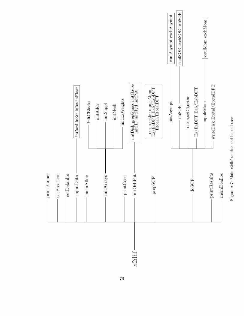
x2d

hf

pri

ntB

anner

setP

reci

sion

setD

efau

lts

inputD

ata

inC

ard

inS

trin

Int

inF

loat

mem

Alloc

init

Arr

ays

init

CB

lock

s

init

Ad

dr

init

Su

pp

l

init

Mes

h

init

ExW

eigh

tspri

ntC

ase

init

Orb

Pot

init

Dis

kp

rep

Gau

ssin

itG

auss

init

HF

init

Hyd

init

Pot

pre

pSC

Fn

orm

orth

om

pol

eMom

Ea/

EaD

FT

Eab

/Eab

DF

TE

tota

l/E

tota

lDF

T

doS

CF

pot

Asy

mp

tco

ulA

sym

pt

exch

Asy

mp

t

doS

OR

cou

lSO

Rex

chSO

Rorb

SO

R

nor

m,s

etC

i,or

tho

Ea/

EaD

FT

Eab

/Eab

DF

T

mp

oleM

omco

ulM

om

exch

Mom

wri

teD

isk

Eto

tal/

Eto

talD

FT

pri

ntR

esult

s

mem

Dea

lloc

Fig

ure

A.7

:M

ain

x2d

hf

rou

tin

ean

dit

sca

lltr

ee

79

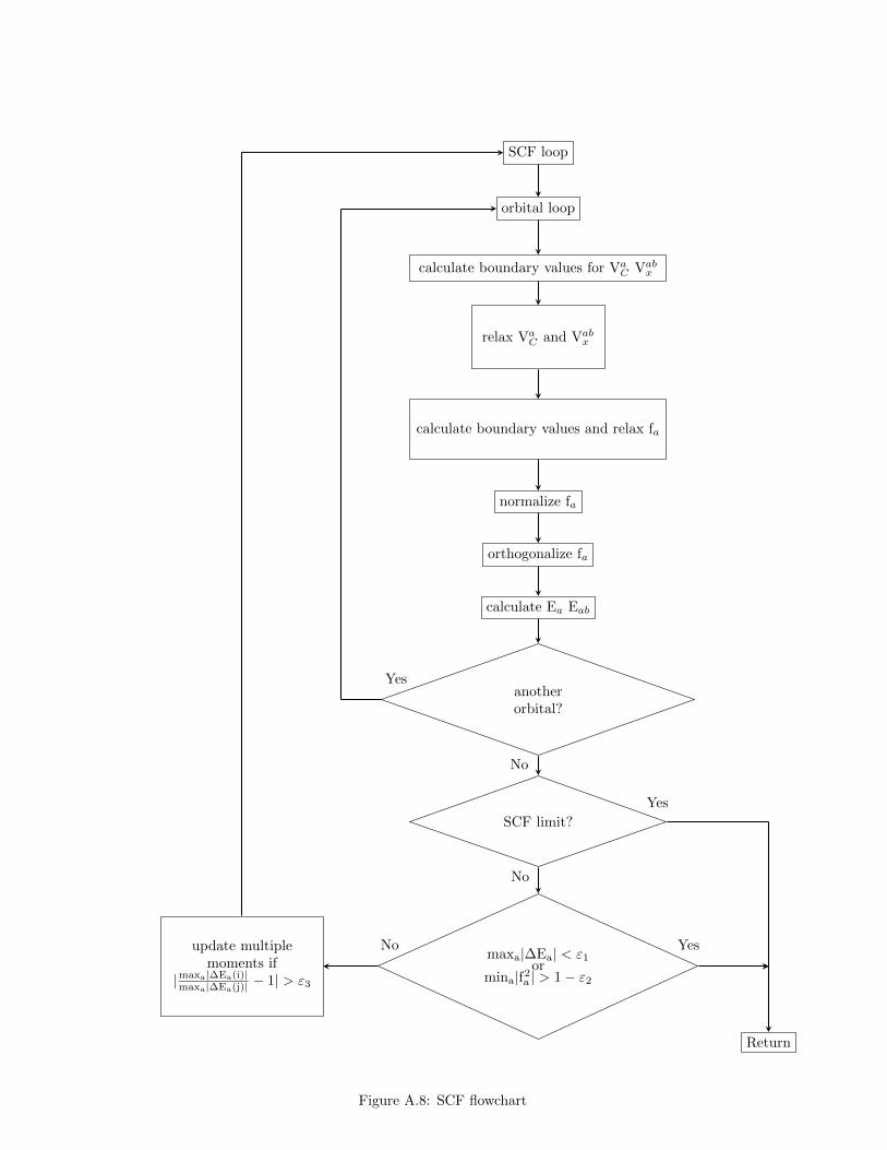
SCF loop

orbital loop

calculate boundary values for VaC Vab

x

relax VaC and Vab

x

calculate boundary values and relax fa

normalize fa

orthogonalize fa

calculate Ea Eab

anotherorbital?

Yes

No

SCF limit?

Yes

No

maxa|∆Ea| < ε1or

mina|f2a | > 1− ε2

YesNo

Return

update multiplemoments if

|maxa|∆Ea(i)|maxa|∆Ea(j)| − 1| > ε3

Figure A.8: SCF flowchart

••

••

••

••

••

••

•

••

••

••

••

••

••

•

••

••

••

••

••

••

•

••

••

••

••

••

••

•

••

••

A ××

××

××

××

××

××

×

••

••

⊗1 ◦

6 ◦11 ◦

16 ◦

21 ◦

26 ◦

31 ◦

36 ◦

??

??

••

••

⊗2 ◦

7 ◦12 ◦

17 ◦

22 ◦

27 ◦

32 ◦

37 ◦

??

??

••

••

⊗3 ◦

8 ◦13 ◦

18 ◦

23 ◦

28 ◦

33 ◦

38 ◦

??

??

••

••

⊗4 ◦

9 ◦14 ◦

19 ◦

24 ◦

29 ◦

34 ◦

39 ◦

??

??

••

••

⊗5 ◦

10 ◦

15 ◦

20 ◦

25 ◦

30 ◦

35 ◦

40 ◦

??

??

••

••

B ××

××

××

××

××

××

×

••

••

••

••

••

••

•

••

••

••

••

••

••

•

••

••

••

••

••

••

•

••

••

••

••

••

••

•

Fig

ure

A.9

:C

olu

mn

-wis

ety

pe

ord

erin

gof

mes

hp

oin

ts.µ

coord

inate

incr

ease

sh

ori

zonta

lly

from

left

tori

gth

an

dν

vert

icall

y,e.

i.th

eb

oun

dar

yp

oints

(0,1

)an

d(π,1

)co

rres

pon

dto

the

posi

tion

of

the

nu

clei

Aan

dB

,re

spec

tive

ly.

81

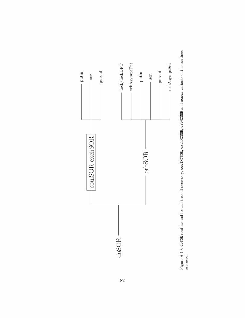
doS

OR

cou

lSO

Rex

chS

OR

pu

tin

sor

pu

tou

t

orb

SO

R

fock

/fock

DF

T

orb

Asy

mp

tDet

pu

tin

sor

pu

tou

t

orb

Asy

mp

tSet

Fig

ure

A.1

0:doSOR

rou

tin

ean

dit

sca

lltr

ee.

Ifn

eces

ssry

,coulMCSOR,exchMCSOR,orbMCSOR

an

dmcsor

vari

ants

of

the

rou

tin

esar

eu

sed

.

82

••

••

••

••

••

••

•

••

••

••

••

••

••

•

••

••

••

••

••

••

•

••

••

••

••

••

••

•

••

••

A ××

××

××

××

××

××

×

••

••

⊗22 ◦

17 ◦

12 ◦

7 ◦2 ◦

27 ◦

32 ◦

37 ◦

??

??

••

••

⊗21 ◦

16 ◦

11 ◦

6 ◦1 ◦

26 ◦

31 ◦

36 ◦

??

??

••

••

⊗23 ◦

18 ◦

13 ◦

8 ◦3 ◦

28 ◦

33 ◦

38 ◦

??

??

••

••

⊗24 ◦

19 ◦

14 ◦

9 ◦4 ◦

29 ◦

34 ◦

39 ◦

??

??

••

••

⊗25 ◦

20 ◦

15 ◦

10 ◦

5 ◦30 ◦

35 ◦

40 ◦

??

??

••

••

B ××

××

××

××

××

××

×

••

••

••

••

••

••

•

••

••

••

••

••

••

•

••

••

••

••

••

••

•

••

••

••

••

••

••

•

Fig

ure

A.1

1:’M

idd

le’

typ

eor

der

ing

of

mes

hp

oin

ts.µ

coord

inate

incr

ease

sh

ori

zonta

lly

from

left

tori

gth

an

dν

vert

icall

y,i.

e.th

eb

oun

dar

yp

oints

(0,1

)an

d(π,1

)co

rres

pon

dto

the

posi

tion

of

the

nu

clei

Aan

dB

,re

spec

tive

ly.

83

× × × × × × × × × × × × ×⊗ ♣ 4 ♠ ♥ |♦| ♣ 4 ♠ ? ? ? ?

⊗ ♦ ♣ 4 ♠ |♥| ♦ ♣ 4 ? ? ? ?

⊗ ♥ ♦ ♣ 4 |♠| ♥ ♦ ♣ ? ? ? ?

⊗ ♠ ♥ ♦ ♣ |4| ♠ ♥ ♦ ? ? ? ?

⊗ |4| |♠| |♥| |♦| |♣| |4| |♠| |♥| | ? | ? ? ?

⊗ ♣ 4 ♠ ♥ |♦| ♣ 4 ♠ ? ? ? ?

⊗ ♦ ♣ 4 ♠ |♥| ♦ ♣ 4 ? ? ? ?

⊗ ♥ ♦ ♣ 4 |♠| ♥ ♦ ♣ ? ? ? ?

⊗ ♠ ♥ ♦ ♣ |4| ♠ ♥ ♦ ? ? ? ?⊗ 4 ♠ ♥ ♦ ♣ 4 ♠ ♥ ? ? ? ?⊗ ♣ 4 ♠ ♥ ♦ ♣ 4 ♠ ? ? ? ?⊗ ♦ ♣ 4 ♠ ♥ ♦ ♣ 4 ? ? ? ?⊗ ♥ ♦ ♣ 4 ♠ ♥ ♦ ♣ ? ? ? ?⊗ ♠ ♥ ♦ ♣ 4 ♠ ♥ ♦ ? ? ? ?⊗ 4 ♠ ♥ ♦ ♣ 4 ♠ ♥ ? ? ? ?⊗ ♣ 4 ♠ ♥ ♦ ♣ 4 ♠ ? ? ? ?⊗ ♦ ♣ 4 ♠ ♥ ♦ ♣ 4 ? ? ? ?⊗ ♥ ♦ ♣ 4 ♠ ♥ ♦ ♣ ? ? ? ?⊗ ♠ ♥ ♦ ♣ 4 ♠ ♥ ♦ ? ? ? ?⊗ 4 ♠ ♥ ♦ ♣ 4 ♠ ♥ ? ? ? ?⊗ ♣ 4 ♠ ♥ ♦ ♣ 4 ♠ ? ? ? ?⊗ ♦ ♣ 4 ♠ ♥ ♦ ♣ 4 ? ? ? ?⊗ ♥ ♦ ♣ 4 ♠ ♥ ♦ ♣ ? ? ? ?⊗ ♠ ♥ ♦ ♣ 4 ♠ ♥ ♦ ? ? ? ?⊗ 4 ♠ ♥ ♦ ♣ 4 ♠ ♥ ? ? ? ?⊗ ♣ 4 ♠ ♥ ♦ ♣ 4 ♠ ? ? ? ?⊗ ♦ ♣ 4 ♠ ♥ ♦ ♣ 4 ? ? ? ?⊗ ♥ ♦ ♣ 4 ♠ ♥ ♦ ♣ ? ? ? ?⊗ ♠ ♥ ♦ ♣ 4 ♠ ♥ ♦ ? ? ? ?× × × × × × × × × × × × ×

Figure A.12: Colouring of mesh points for the MCSOR method and [31×13] grid when17-point cross-like stencil is used for discretization.

84