a fictitious domain approach to the direct numerical simulation of incompressible viscous flow past...
TRANSCRIPT

Journal of Computational Physics169,363–426 (2001)
doi:10.1006/jcph.2000.6542, available online at http://www.idealibrary.com on
A Fictitious Domain Approach to the DirectNumerical Simulation of IncompressibleViscous Flow past Moving Rigid Bodies:
Application to Particulate Flow
R. Glowinski,∗ T. W. Pan,∗ T. I. Hesla,† D. D. Joseph,† and J. P´eriaux‡∗Department of Mathematics, University of Houston, Houston, Texas 77204-3476;†Aerospace Engineering and
Mechanics, University of Minnesota, 107 Ackerman Hall, 110 Union Street, Minneapolis, Minnesota 55455;and‡Dassault Aviation, 1 Rue Charles Blum, Cedex 300, 92552 Saint Cloud, France
E-mail: [email protected], [email protected], [email protected],[email protected], [email protected]
Received December 16, 1999; revised April 26, 2000
In this article we discuss a methodology that allows the direct numerical simula-tion of incompressible viscous fluid flow past moving rigid bodies. The simulationmethods rest essentially on the combination of:
(a) Lagrange-multiplier-based fictitious domain methods which allow the fluidflow computations to be done in a fixed flow region.
(b) Finite element approximations of the Navier–Stokes equations occurringin the global model.
(c) Time discretizations by operator splitting schemes in order to treat optimallythe various operators present in the model.
The above methodology is particularly well suited to the direct numerical simulationof particulate flow, such as the flow of mixtures of rigid solid particles and incom-pressible viscous fluids, possibly non-Newtonian. We conclude this article with thepresentation of the results of various numerical experiments, including the simulationof store separation for rigid airfoils and of sedimentation and fluidization phenomenain two and three dimensions. c© 2001 Academic Press
Key Words: fictitious domain methods; finite element methods; distributedLagrange multipliers; Navier–Stokes equations; particulate flow; liquid–solid mix-tures; store separation; sedimentation; fluidization; Rayleigh–Taylor instabilities.
363
0021-9991/01 $35.00Copyright c© 2001 by Academic Press
All rights of reproduction in any form reserved.

364 GLOWINSKI ET AL.
1. INTRODUCTION
The main goal of this article is to discuss a methodology well suited to the direct numeri-cal simulation of (possibly non-Newtonian) incompressible viscous flow past moving rigidbodieswhen the motion of the bodies is not known in advancebut results from the hydro-dynamical coupling and external forces such as gravity and collisions (or near collisions).The methodology discussed here relies on several ingredients, the pivotal ones being:
• A fictitious domain method which allows the flow computation to be done on a fixedspace region which contains the moving rigid bodies.• Lagrange multipliers defined on the regions occupied by the rigid bodies, to match
over these regions the fluid flow and rigid body motion velocities.• A simple but effcient strategy to take into account body/body and body/wall colli-
sions (or near collisions).• Finite element approximations taking advantage of a global variational formulation
(of the virtual power principle type) of the coupled flow–rigid body motion.• Time discretizations by operator splitting in order to treat separately and (in princi-
ple) optimally the various operators associated to the physics and numerics of the compu-tational model.
In this article, the above methods will be applied to the direct numerical simulation ofvarious incompressible Newtonian and non-Newtonian viscous flows past moving rigidbodies in two and three dimensions. These test problems will include the simulation ofstore separationfor rigid airfoils and ofsedimentationand fluidization phenomena forsmall and large (>103) populations of particles.
An alternative approach to the methodology discussed in this article can be found inRef. [1], in the present issue of theJournal of Computational Physics; it is based on theArbitrary Lagrange–Eulermethodology with the flow computed, with a moving mesh ona time-varying region (see [1] and the references therein for details).
The present article reviews (and improves) methods and results discussed in Refs. [2]–[8].
2. MODELING OF THE FLUID–RIGID BODY INTERACTION
LetÄ ⊂ Rd (d = 2, 3) be a space region; we suppose thatÄ is filled with anincompress-ible viscous fluidof densityρ f and that it containsJ moving rigid bodiesB1, B2, . . . , BJ
(see Fig. 2.1 for a particular case whered = 2 andJ = 3). We denote byn the unit normalvector on the boundary ofÄ\⋃J
j=1B j , pointing outward to the flow region. Assuming thatthe only external force acting on the mixture isgravity, then, betweencollisions(assumingthat collisions take place), thefluid flow is modeled by theNavier–Stokes equations
ρ f
[∂u∂t+ (u ·∇)u
]= ρ f g+∇ · σ in Ä
∖ J⋃j=1
Bj (t),
∇ · u = 0 inÄ
∖ J⋃j=1
Bj (t), (2.1)
u(x, 0) = u0(x), ∀x ∈ Ä∖ J⋃
j=1
Bj (0), with∇ · u0 = 0,

FICTITIOUS DOMAIN APPROACH 365
FIG. 2.1. An example of a two-dimensional flow region with three rigid bodies.
to be completed by
u = g0 on0 with∫0
g0 · n d0 = 0 (2.2)
and by the followingno-slip boundary conditionon the boundary∂Bj of Bj ,
u(x, t) = V j (t)+ ω j (t)×−−−→G j (t)x, ∀x ∈ ∂Bj (t), (2.3)
where, in (2.3),V j (resp.,ω j ) denotes thevelocity of the center of massG j (resp., theangular velocity) of the j th body, for j = 1, . . . , J. In (2.1), thestress-tensorσ verifies
σ = τ − pI , (2.4)
typical situations forτ being
τ = 2νD(u) = ν(∇u+∇ut ) (Newtonian case), (2.5)
τ is a nonlinear function of∇u (non-Newtonian case). (2.6)
The motion of the rigid bodies is modeled by theNewton–Eulerequations
M jdV j
dt= M j g+ F j ,
(2.7)
I jdω j
dt+ ω j × I jω j = T j ,
for j = 1, . . . , J, where in (2.7),
• M j is themassof the j th rigid body,• I j is theinertia tensorof the j th rigid body,• F j is the resultant of thehydrodynamical forcesacting on thej th body, i.e.,
F j = (−1)∫∂B j
σn d(∂Bj ), (2.8)
• T j is the torque atG j of the hydrodynamical forces acting on thej th body, i.e.,
T j = (−1)∫∂B j
−−−→G j x ×σn d(∂Bj ), (2.9)

366 GLOWINSKI ET AL.
• and we have
dG j
dt= V j . (2.10)
Equations (2.7) to (2.10) have to be completed by the followinginitial conditions:
Bj (0) = B0 j , G j (0) = G0 j , V j (0) = V0 j , ω j (0) = ω0 j , ∀ j = 1, . . . , J.
(2.11)
Remark 2.1. If Bj is made of ahomogeneousmaterial ofdensityρ j , we have
M j = ρ j
∫Bj
dx, I j =
I11, j −I12, j −I13, j
−I12, j I22, j −I23, j
−I13, j −I23, j I33, j
, (2.12)
where, in (2.12),dx = dx1 dx2 dx3 and
I11, j = ρ j
∫Bj
(x2
2 + x23
)dx, I22, j = ρ j
∫Bj
(x2
3 + x21
)dx, I33, j = ρ j
∫Bj
(x2
1 + x22
)dx,
I12, j = ρ j
∫Bj
x1x2 dx, I23, j = ρ j
∫Bj
x2x3 dx, I13, j = ρ j
∫Bj
x1x3 dx.
Remark 2.2. If the flow–rigid body motion is two-dimensional, or ifBj is a sphericalbody made of ahomogeneousmaterial, then the nonlinear termω j × I jω j vanishes in (2.7).
Remark 2.3. Suppose that the rigid bodies do not touch att = 0; then it has been shownby B. Desjardins and M. Esteban (Ref. [9]) that the system of equations modeling the flowof the above fluid–rigid body mixture has a (weak) solution on the time interval [0, t∗),t∗(>0) depending on the initial conditions; uniqueness is an open problem.
3. A GLOBAL VARIATIONAL FORMULATION OF THE FLUID–SOLID
INTERACTION VIA THE VIRTUAL POWER PRINCIPLE
We suppose, in this section, that the fluid isNewtonianof viscosityν. Let us denote byB(t) the space region occupied at timet by the rigid bodies; we have thusB(t) = ⋃J
j=1Bj (t).To obtain avariational formulationfor the system of equations described in Section 2, weintroduce the followingfunctional spaceof compatible test functions:
W0(t) ={{v,Y,θ} | v ∈ (H1(Ä\B(t)))d, v = 0 on0,
Y = {Y j }Jj=1, θ = {θ j }Jj=1, with Y j ∈ Rd,θ j ∈ R3, (3.1)
v(x, t) = Y j + θ j ×−−−→G j (t)x on ∂Bj (t), ∀ j = 1, . . . , J
}.
In (3.1) we haveθ j = {0, 0, θ j } if d = 2.

FICTITIOUS DOMAIN APPROACH 367
Applying thevirtual power principleto thewholemixture (i.e., to the fluidandthe rigidbodies) yields theglobalvariational formulation
ρf
∫Ä\B(t)
[∂u∂t+ (u ·∇)u
]· v dx+ 2ν
∫Ä\B(t)
D(u) : D(v) dx
−∫Ä\B(t)
p∇ · v dx+J∑
j=1
M j V j · Y j +J∑
j=1
(I j ω j + ω j × I jω j ) · θ j (3.2)
= ρf
∫Ä\B(t)
g · v dx+J∑
j=1
M j g · Y j , ∀{v,Y, θ} ∈ W0(t),
∫Ä\B(t)
q∇ · u(t) dx = 0, ∀q ∈ L2(Ä\B(t)), (3.3)
u(t) = g0(t) on0, (3.4)
u(x, t) = V j (t)+ ω j (t)×−−−→G j (t)x, ∀x ∈ ∂Bj (t), ∀ j = 1, . . . , J, (3.5)
dG j
dt= V j , (3.6)
to be completed by theinitial conditions
u(x, 0) = u0(x), ∀x ∈ Ä\B(0), (3.7)
Bj (0)= B0 j , G j (0)=G0 j , V j (0)=V0 j , ω j (0)=ω0 j , ∀ j = 1, . . . , J. (3.8)
In relations (3.2) to (3.8):
• We have denoted functions such asx→ ϕ(x, t) by ϕ(t).• We have used the following notation:
a · b =d∑
k=1
akbk, ∀a= {ak}dk=1, b = {bk}dk=1,
A : B =d∑
k=1
d∑l=1
aklbkl , ∀A = (akl)1≤k,l≤d,B = (bkl)1≤k,l≤d.
• It is reasonable to assume thatu(t) ∈ (H1(Ä\B(t)))d and p(t) ∈ L2(Ä\B(t)).• We haveω j (t) = {0, 0, ω j (t)} if d = 2.
Formulations such as (3.2)–(3.8) (or closely related ones) have been used by several authors(see, e.g., [1], [10]–[12]) to simulate particulate flow viaarbitrary Lagrange–Euler(ALE)methods using moving meshes (actually, formulation (3.2)–(3.8) has been used in [9] toprove the existence of a local in time weak solution to problem (2.1)–(2.5), (2.7), (2.11)).Our goal in this article is to discuss an alternative based onfictitious domain methods(alsocalleddomain embeddingmethods). The main advantage of this new (in the context ofparticulate flow) approach is the possibility of achieving the flow-related computations ona fixedspace region, allowing thus the use of a fixed (finite difference or finite element)mesh, which is a significant simplification.

368 GLOWINSKI ET AL.
4. A DISTRIBUTED LAGRANGE-MULTIPLIER-BASED FICTITIOUS
DOMAIN FORMULATION
In general terms our goal is to find a methodology in which
(a) a fixed mesh can be used for flow computations,(b) the rigid body positions are obtained from the solution of the Newton–Euler equa-
tions of motion, and(c) The time discretization is done by operator splitting methods in order to treat
individually the various operators occurring in the mathematical model.
To achieve such a goal we proceed as follows:
(i) We fill the rigid bodies with the surrounding fluid.(ii) We assume that the fluid inside each body has a rigid body motion.(iii) We use (i) and (ii) to modify the variational formulation (3.2)–(3.8).(iv) We force the rigid body motion inside each moving body via a Lagrange multiplier
defined (distributed) over the body.(v) We combine (iii) and (iv) to derive a variational formulation involving Lagrange
multipliers to force the rigid body motion inside the moving bodies.
We suppose (for simplicity) that each rigid bodyBj is made of ahomogeneous materialof densityρ j ; then, taking into account the fact that any rigid body motion velocity fieldvverifies∇ · v = 0 andD(v) = 0, steps (i) to (iii) yield the following variant of formulation(3.2)–(3.8):
For a.e.t > 0, findu(t), p(t), {V j (t),G j (t),ω j (t)}Jj=1, such that
ρf
∫Ä
[∂u∂t+ (u ·∇)u
]· v dx−
∫Ä
p∇ · v dx+ 2ν∫Ä
D(u) : D(v) dx
+J∑
j=1
(1− ρ f /ρ j )
[M j
dv j
dt· Y j +
(I j
dω j
dt+ ω j × I jω j
)· θ j
](4.1)
= ρf
∫Ä
g · v dx+J∑
j=1
(1− ρ f /ρ j )M j g · Y j , ∀{v,Y,θ} ∈ W0(t),∫Ä
q∇ · u dx = 0, ∀q ∈ L2(Ä), (4.2)
u = g0 on0, (4.3)
u(x, t) = V j (t)+ ω j (t)×−−−→G j (t)x, ∀x ∈ Bj (t), ∀ j = 1, . . . , J, (4.4)
dG j
dt= V j , (4.5)
Bj (0)= B0 j , V j (0)=V0 j , ω j (0)=ω0 j , G j (0)=G0 j , ∀ j = 1, . . . , J,
(4.6)
u(x, 0)= u0(x), ∀x ∈ Ä∖ J⋃
j=1
B0 j and u(x, 0) = V0 j + ω0 j ×−−−→G0 j x ,
∀x ∈ B0 j (4.7)

FICTITIOUS DOMAIN APPROACH 369
with, in relation (4.1), spaceW0(t) defined by
W0(t) ={{v,Y,θ} | v ∈ (H1
0 (Ä))d, Y = {Y j }Jj=1,θ = {θ j }Jj=1,with Y j ∈ Rd,
θ j ∈ R3, v(x, t) = Y j + θ j ×−−−→G j (t)x in Bj (t), ∀ j = 1, . . . , J
}.
Concerningu and p, it makes sense to assume thatu(t) ∈ (H1(Ä))d and p(t) ∈ L2(Ä).
In order to relax therigid body motion constraint(4.4), we are going to employ a family{λ j }Jj=1 of Lagrange multipliersso thatλ j (t) ∈ 3 j (t) with
3 j (t) = (H1(Bj (t)))d, ∀ j = 1, . . . , J. (4.8)
We obtain, thus, the followingfictitious domain formulation with Lagrange multipliers:
For a.e.t > 0, findu(t), p(t), {V j (t),G j (t),ω j (t),λ j (t)}Jj=1, such that
u(t) ∈ (H1(Ä))d, u(t) = g0(t) on0, p(t) ∈ L2(Ä),(4.9)
V j (t) ∈ Rd,G j (t) ∈ Rd,ω j (t) ∈ R3,λ j (t) ∈ 3 j (t), ∀ j = 1, . . . , J,
and
ρ f
∫Ä
[∂u∂t+ (u ·∇)u
]· v dx−
∫Ä
p∇ · v dx+ 2ν∫Ä
D(u) : D(v) dx
−J∑
j=1
〈λ j , v− Y j − θ j ×−−−→G j x 〉 j +
J∑j=1
(1− ρ f /ρ j )M jdV j
dt· Y j
(4.10)
+J∑
j=1
(1− ρ f /ρ j )
(I j
dω j
dt+ ω j × I jω j
)· θ j = ρ f
∫Ä
g · v dx
+J∑
j=1
(1− ρ f /ρ j )M j g · Y j , ∀v ∈ (H10 (Ä)
)d, ∀Y j ∈ Rd, ∀θ j ∈ R3,
∫Ä
q∇ · u dx = 0, ∀q ∈ L2(Ä), (4.11)
〈µ j , u(t)−V j (t)−ω j (t)×−−−→G j (t)x〉 j = 0, ∀µ j ∈ 3 j (t), ∀ j = 1, . . . , J, (4.12)
dG j
dt= V j , ∀ j = 1, . . . , J, (4.13)
V j (0) = V0 j , G j (0)=G0 j , ω j (0) = ω0 j , Bj (0) = B0 j , ∀ j = 1, . . . , J,
(4.14)
u(x, 0) = u0(x), ∀x ∈ Ä∖ J⋃
j=1
B0 j and u(x, 0) = V0 j + ω0 j ×−−−→G0 j x , ∀x ∈ B0 j .
(4.15)
The two most natural choices for〈·, ·〉 j are defined by
〈µ, v〉 j =∫
Bj (t)
(µ · v+ δ2
j∇µ :∇v)
dx, ∀µ andv ∈ 3 j (t), (4.16)

370 GLOWINSKI ET AL.
〈µ, v〉 j =∫
Bj (t)
(µ · v+ δ2
j D(µ) : D(v))
dx, ∀µ andv ∈ 3 j (t), (4.17)
with δ j as acharacteristic length(the diameter ofBj , for example). Other choices arepossible, such as
〈µ, v〉 j =∫∂Bj (t)
µ · v d(∂Bj )+ δ j
∫Bj (t)∇µ :∇v dx, ∀µ andv ∈ 3 j (t),
or
〈µ, v〉 j =∫∂Bj (t)
µ · v d(∂Bj )+ δ j
∫Bj (t)
D(µ) : D(v) dx, ∀µ andv ∈ 3 j (t).
Remark 4.1. The fictitious domain approach, described above, has clearly many simi-larities with theimmersed boundaryapproach of C. Peskin (see Refs. [13]–[16]). However,the systematic use ofLagrange multipliersseems to be new in this context. Another majordifference is the fact that in our approach the boundary of the moving rigid bodies does notplay the fundamental role it plays in the Peskin’s approach.
Remark 4.2. An approach with some similarities to ours has been developed byS. Schwarzeret al. (see Ref. [17]) in a finite difference framework. In the above refer-ence (dedicated to the simulation of particulate flow), the interaction between the rigidbody and the fluid is forced via apenalty method, instead of the multiplier technique used inthe present article; also, minor particle–particle penetration is allowed and no enforcementof the rigid body motion inside the region occupied by the particle is done.
Remark 4.3. In order to force the rigid body motion inside the moving rigid bodieswe can use the fact thatv defined overÄ is a rigid body motion velocity field inside eachmoving rigid body if and only ifD(v) = 0 in Bj (t), ∀ j = 1, . . . , J; i.e.,∫
Bj (t)D(v) : D(µ) dx = 0, ∀µ ∈ 3 j (t), ∀ j = 1, . . . , J. (4.18)
A computational method based on this approach is discussed in [18].
Remark 4.4. Since, in (4.10),u is divergence freeand satisfies Dirichlet boundaryconditions on0, we have
2∫Ä
D(u) : D(v) dx =∫Ä
∇u :∇v dx, ∀v ∈ (H10 (Ä)
)d, (4.19)
a substantial simplification indeed, from acomputational point of view, which is anotherplus for the fictitious domain approach used here.
Remark 4.5. Using high-energy physics terminology, the multiplierλ j can be viewedas agluonwhose role is to force the rigidity insideBj by matching the velocity fields oftwo continua. More precisely, the multipliersλ j are mathematical objects of themortartype, very close to those used indomain decomposition methodsto match local solutionsat interfaces or on overlapping regions (see Ref. [19]). Indeed, theλ j in the present articlehave genuine mortar properties since their role is to force a fluid to behave like a rigid solidinside the space region occupied by the moving bodies.

FICTITIOUS DOMAIN APPROACH 371
5. ON THE TREATMENT OF COLLISIONS
In the above sections, we have considered the motion of fluid/rigid body mixtures andhave given various mathematical models of this phenomenon, assuming that there was norigid body/rigid body or boundary/rigid body collisions. Actually, with the mathematicalmodel that we have considered it is not known if collisions can take place in finite time(in fact several scientists strongly believe that lubrication forces prevent these collisionsin the case of viscous fluids). However, collisions take place in nature and also in actualnumerical simulations if special precautions are not taken. In the particular case of rigidbodies moving in a viscous fluid, under the effect of gravity and hydrodynamical forces, weshall assume that the collisions taking place aresmoothones in the sense that if two rigidbodies collide (resp., if a rigid body hits the boundary), the rigid body velocities (resp., therigid body and boundary velocities) coincide at the points of contact. From the smooth natureof these collisions the only precaution to be taken will be to avoid overlapping of the regionsoccupied by the rigid bodies. To achieve this goal, we include in the right-hand sides oftheNewton–Euler equations(2.7) modeling the rigid body motion ashort-range repulsiveforce. If we consider the particular case of rigid bodiescircular (in two-dimensions) orspherical(in three-dimensions), and ifBi andBj are two such rigid bodies, with radiiRi
and Rj and centers of massGi andG j , we shall require the repulsion force−→Fi j between
Bi andBj to satisfy the following properties:
(i) to be parallel to−−−→Gi G j ,
(ii) to verify
| −→Fi j | = 0 if di j ≥ Ri + Rj + ρ,(5.1)
| −→Fi j | = ci j /ε if di j = Ri + Rj ,
with di j = |−−−→Gi G j |, ci j as ascaling factor, andε as a “small” positive number, and
(iii) | −→Fi j | has to behave as in Fig. 5.1 for
Ri + Rj ≤ di j ≤ Ri + Rj + ρ.
FIG. 5.1. Repulsion force behavior.

372 GLOWINSKI ET AL.
Parameterρ is the range of the repulsion force; for the simulations discussed in thefollowing sections, we have takenρ ' hÄ (hÄ is the space discretization stepused forapproximating thevelocity). Boundary/rigid body collisions can be treated in a similar way.
Remark 5.1. For those readers wondering how to adjusthÄ andε, we would like tomake the following comments: clearly, the space discretization parameterhÄ is adjusted sothat the finite element approximation can resolve the boundary and shear layers occurringin the flow. Next, it is clear thatρ can be taken of the order ofhÄ. The choice ofε is moresubtle; suppose that
−→Fi j is defined by
−→Fi j = ci j
ε
((di j − Ri − Rj − ρ
ρ
)−)2−−−→Gi G j
di j, (5.2)
where, in (5.2), we have used the notationξ− = max(0,−ξ ). Denoting, as usual, the di-mension of quantityX by [X], ε will be a dimensionalif and only if ci j has the dimensionof a force, i.e., [ci j ] = MLT−2.
In order to linkε andρ, we are going to consider the simple model problem where amaterial point of massm is dropped from heightz= H , without initial velocity, abovea rigid obstacle located atz= 0 and falls under the effect of gravity. Assuming that thecollision is treated as above bypenaltyand a natural choice for the scaling parametercbeingmg, the motion of the point is described bymz− mg
ερ2((z− ρ)−)2 = −mg,
z(0) = H, z(0) = 0.(5.3)
A long asz≥ ρ the equation of motion reduces toz= −g, which implies that the materialpoint reachesz= ρ for the first timeat t = tρ , with
tρ =√
2(H − ρ)g
, (5.4)
the velocityz(tρ) being given by
z(tρ) = −√
2g(H − ρ). (5.5)
For z≤ ρ the differential equation in (5.3) can also be written as
z− g
ερ2(z− ρ)2+ g = 0. (5.6)
Multiplying both sides of the differential equation (5.6) byz, and observing thatdz/dt =d(z− ρ)/dt, yields
d
dt
[1
2z2− g
3ερ2(z− ρ)3+ g(z− ρ)
]= 0. (5.7)
It follows from (5.5) and (5.7) that as long asz(t) ≤ ρ, we have
1
2z(t)2− g
3ερ2(z(t)− ρ)3+ g(z(t)− ρ) = g(H − ρ). (5.8)
FICTITIOUS DOMAIN APPROACH 373
The material point reaches its minimal heightzm for tm such thatzm(t) = 0. It follows thusfrom (5.8) thatzm verifies
zm− ρ − (zm− ρ)3/(3ερ2) = H − ρ. (5.9)
Let us denote themaximal penetration distanceρ − zm by δ; we have then (from (5.9))
δ3/(3ερ2)− δ = H − ρ. (5.10)
We are going to use relation (5.10) to explore several scenarios:
(i) Suppose thatH = ρ; it follows then from (5.10) that
δ =√
3ερ, (5.11)
which implies in turn that to haveδ/ρ ¿ 1 we need to take√ε ¿ 1, i.e., δ/ρ “small”
impliesε “very small.” Typically,δ/ρ ' 10−2 impliesε ' 10−4.(ii) Suppose now thatH À ρ. Since we wantδ/ρ ¿ 1, it follows from (5.10) that
δ3/(3ερ2) ' H,
i.e.,
δ/ρ ' (3ε)1/3(H/ρ)1/3. (5.12)
Suppose that, for example,H/ρ = 102 and that we want to takeδ/ρ ' 10−2; it follows thenfrom (5.11) that we need to takeε ' 10−8, i.e.,δ/ρ “small” implies ε “very very small.”
Returning to (5.2), let us say that scenario (ii) will be encountered (in some sense) if thefluid surrounding the rigid bodies isinviscid, implying possible violent collisions. Scenario(i) corresponds clearly to a soft collision sinceρ ' hÄ, and we shall assume that it is thekind of situation which prevails if the fluid is sufficiently viscous and the ratioρ j /ρf is nottoo large, i.e.,ρ j /ρf of the order of 1,∀ j = 1, . . . , J. On the basis of these assumptionswe have always takenε ' h2
Ä for the calculations to be presented in Section 8.
Remark 5.2. In order to treat the collisions, we can use repulsion forces derived bytruncation of theLennard–Jonespotentials frommolecular dynamics(see, e.g., [20] forthese notions from molecular chemistry); this approach is commonly used by physico-chemists to treat collisions in solvents containing “large” particles (whose characteristicsizes are a few micrometers at least).
Remark 5.3. Penalty methods, closely related to those discussed just above, have been(and still are) used by mechanical engineers for the numerical treatment of contact problems.A fundamental reference on these topics is the book by Kikuchi and Oden (Ref. [21]; seealso the references therein). The above reference contains comparisons between resultsobtained by application of the Hertz contact theory and results obtained by penalty methods.According to [21], penalty methods allow the solution of contact problems for which Hertztheory is no longer valid.

374 GLOWINSKI ET AL.
FIG. 6.1. Subdivision of a triangle ofT2h.
6. FINITE ELEMENT APPROXIMATION
For simplicity, we assume thatÄ ⊂ R2 (i.e.,d = 2) and is polygonal; we have thenω(t) ={0, 0, ω(t)} andθ = {0, 0, θ} with ω(t) andθ ∈ R. Concerning thespace approximationof problem (4.9)–(4.15) by afinite element method, we shall proceed as follows:
With h(=hÄ) as aspace discretization step, we introduce a finite element triangulationTh of Ä and a triangulationT2h twice coarser (in practice we should constructT2h first andthenTh by joining the midpoints of the edges ofT2h, dividing thus each triangle ofT2h intofour similar subtriangles, as shown in Fig. 6.1).
We approximate then(H1(Ä))2, (H10 (Ä))
2, andL2(Ä) by the finite dimensional spaces
Vh = {vh | vh ∈ (C0(Ä))2, vh|T ∈ P1× P1, ∀T ∈ Th}, (6.1)
V0h = {vh | vh ∈Vh, vh = 0 on0}, (6.2)
and
L2h = {qh | qh ∈ C0(Ä),qh|T ∈ P1, ∀T ∈ T2h}, (6.3)
respectively; in (6.1)–(6.3),P1 is the space of the polynomials in two variables of degree≤1. Let Bjh(t) be a polygonal domain inscribed inBj (t) and letT j
h (t) be a finite elementtriangulation ofBjh(t), like the one shown in Fig. 6.2, whereBj is a disk.
FIG. 6.2. Triangulation of a disk.

FICTITIOUS DOMAIN APPROACH 375
A finite dimensional space approximating3 j (t) is
3 jh(t) ={µh | µh ∈ (C0(Bjh(t)))
2,µh|T ∈ P1× P1, ∀T ∈ T jh (t)
}. (6.4)
An alternative to3 jh(t) defined by (6.4) is as follows: let{xi }Nj
i=1 be a set of points fromBj (t) which coverBj (t) (uniformly, for example); we define then
3 jh(t) ={µh | µh =
Nj∑i=1
µi δ(x− xi ),µi ∈ R2, ∀i = 1, . . . , Nj
}, (6.5)
where δ(·) is the Dirac measure atx = 0. Then, instead of the scalar product of(H1(Bjh(t)))2, we shall use〈·, ·〉 jh defined by
〈µh, vh〉 jh =Nj∑
i=1
µi · vh(xi ), ∀µh ∈ 3 jh(t), vh ∈ Vh. (6.6)
The approach based on (6.5) and (6.6) makes little sense for the continuous problem, but itis meaningful for the discrete problem; it amounts to forcing the rigid body motion ofBj (t)via acollocation method. A similar technique has been used to enforce Dirichlet boundaryconditions, by F. Bertrandet al. (Ref. [22]).
Remark 6.1. The bilinear form in (6.6) has definitely the flavor of adiscrete L2(Bj (t))-scalar product. Let us insist on the fact that taking3 j (t) = (L2(Pj (t)))2 and then
〈µ, v〉 j =∫
Bj (t)µ · v dx, ∀µ andv ∈ 3 j (t)
makes no sense for the continuous problem. On the other hand, it makes sense for the finiteelement variants of (4.9)–(4.15), but do not expectλ jh(t) to converge to anL2-function ash→ 0 (it will converge to some element of the dual space((H1(Bj (t)))2)′ of (H1(Bj (t)))2.
Using the above finite dimensional spaces leads to the following approximation of prob-lem (4.9)–(4.15):
For t > 0 finduh(t), ph(t), {V j (t),G jh(t), ω j (t),λ jh(t)}Jj=1 such that{uh(t) ∈ Vh, ph(t) ∈ L2
h,
V j (t) ∈ R2, G jh(t) ∈ R2, ω j (t) ∈ R,λ jh(t) ∈ 3 jh(t), ∀ j = 1, . . . , J,(6.7)
and
ρ f
∫Ä
[∂uh
∂t+ (uh ·∇)uh
]· v dx−
∫Ä
ph∇ · v dx+ 2ν∫Ä
D(uh) : D(v) dx
+J∑
j=1
(1− ρ f /ρ j )M jdV j
dt· Y j +
J∑j=1
(1− ρ f /ρ j )I jdω j
dtθ j
−J∑
j=1
〈λ jh, v− Y j − θ j ×−−−→G jhx 〉 jh = ρ f
∫Ä
g · v dx
+J∑
j=1
(1− ρ f /ρ j )M j g · Y j , ∀v ∈ V0h, ∀Y j ∈ R2, ∀θ j ∈ R,
(6.8)
376 GLOWINSKI ET AL.
∫Ä
q∇ · uh(t) dx = 0, ∀q ∈ L2h, (6.9)
uh = g0h on0, (6.10)
〈µ jh, uh(t)− V j (t)− ω j (t)×−−−−→G jh(t)x〉 jh = 0, ∀µ jh ∈ 3 jh(t), ∀ j = 1, . . . , J,
(6.11)
dG jh
dt= V j , ∀ j = 1, . . . , J, (6.12)
V j (0) = V0 j , G jh(0) = G0 jh, ω j (0) = ω0 j , Bjh(0) = B0 jh,
∀ j = 1, . . . , J, (6.13)
uh(x, 0) = u0h(x), ∀x ∈ Ä∖ J⋃
j=1
B0 jh, uh(x, 0) = V0 j + ω0 j ×−−−→G0 jhx,
∀x ∈ B0 jh . (6.14)
In (6.10),g0h is an approximation ofg0 belonging to
γVh = {zh | zh ∈ (C0(0))2, zh = zh|0 with zh ∈ Vh}
and verifying∫0
g0h · n d0 = 0.
Remark 6.2. Thediscrete pressurein (6.7)–(6.14) is defined within to an additive con-stant. In order to “fix” the pressure, we shall require it to verify∫
Ä
ph(t) dx = 0, ∀t > 0,
i.e., ph(t) ∈ L20h with L2
0h defined by
L20h =
{qh | qh ∈ L2
h,
∫Ä
qh dx = 0
}.
Remark 6.3. From a practical point of view, the semidiscrete model (6.7)–(6.14) isincomplete since we still have to include thevirtual power associated to thecollisionforces. Assuming that the rigid bodies are circular (d = 2) or spherical (d = 3), we shalladd to the right-hand side of Eq. (6.8) the term
J∑j=1
Frj · Y j , (6.15)
where the repulsion forceFrj is defined as in Section 5. If the rigid bodies are noncircular or
nonspherical we shall have to take into account the virtual power associated to the torqueof the collision forces.
Remark 6.4. Concerning the definition of themultiplier space3 jh(t), several optionsare possible:
(i) If Bj is rotationally invariant(this will be the case for a circular or a spherical rigidbody) we define3 jh(t) from the triangulationT j
h (t) obtained fromT jh (0) by translation.

FICTITIOUS DOMAIN APPROACH 377
(ii) If Bj is not rotationally invariantwe can define3 jh(t) from a triangulationT jh (t)
rigidly attachedto Bj .(iii) We can also define3 jh(t) from the set of points
6 jh(t) = 6vjh(t) ∪6σ
jh(t), (6.16)
where, in (6.16),6vjh(t) is the set of vertices of the velocity gridTh which are contained in
Bj (t), and where6σjh(t) is a set of control points located∂Bj (t). This “hybrid” approach is
(relatively) easy to implement and is particularly well suited to those situations where theboundary∂Bj has corners or edges.
Remark 6.5. In relation (6.8), we can replace 2∫Ä
D(uh) : D(v) dx by∫Ä∇uh :∇v dx,
by taking Remark 4.4 into account.
Remark 6.6. Let hÄ (resp.,h j ) be the mesh size associated to the velocity meshTh
(resp., to the rigid body meshT jh ); then a relation such as
hÄ < χ j h j < h j < 2hÄ, (6.17)
with 0< χ j < 1, seems to be needed, from a theoretical point of view, in order to sat-isfy some kind ofstability conditionof the Brezzi–Babuskatype (for generalities on theapproximation of mixed variational problems, such as (4.9)–(4.15), involvingLagrangemultipliers, see, for example, the publications by F. Brezzi and M. Fortin (Ref. [23]) and J.E. Roberts and J. M. Thomas (Ref. [24])), actually, takingh j = hÄ seems to work fine inpractice.
Remark 6.7. In order to avoid the solution at each time step of complicatedtriangulationintersection problems, we advocate the use of
〈λ jh,5 j v− Y j − θ j ×−−−−→G jh(t)x〉 jh (6.18)
(resp.,
〈µ jh,5 j uh(t)− V j (t)− ω j (t)×−−−−→G jh(t)x〉 jh) (6.19)
in (6.8) (resp., (6.11)), instead of
〈λ jh, v− Y j − θ j ×−−−−→G jh(t)x〉 jh (6.20)
(resp.,
〈µ jh, uh(t)− V j (t)− ω j (t)×−−−−→G jh(t)x〉 jh),
where, in (6.18) and (6.19),5 j : (C0(Ä))2→3 jh(t) is thepiecewise linear interpolationoperatorwhich to each functionw belonging to(C0(Ä))2 associates the unique element of3 jh(t) defined from the values taken byw at the vertices ofT j
h (t).

378 GLOWINSKI ET AL.
Remark 6.8. In general, the functionu(t) has no more than the(H3/2(Ä))2-regularity.This low regularity implies that we can not expect more thanO(h3/2) for the approximationerror‖uh(t)− u(t)‖(L2(Ä))2 andO(h1/2) for the approximation error|uh(t)− u(t)|(H1(Ä))2
(see Ref. [25]).
7. TIME DISCRETIZATION BY OPERATOR SPLITTING
7.1. Generalities
Following A. Chorin (Refs. [26]–[28]), most “modern” Navier–Stokes solvers are basedonoperator splittingschemes (see, e.g., Refs. [29], [30]) in order to force the incompress-ibility condition via a Stokes solver or aL2-projection method. This approach still appliesto the initial value problem (6.7)–(6.14), which contains four numerical difficulties to eachof which can be associated a specific operator, namely,
(a) the incompressibility condition and the related unknown pressure,(b) an advection–diffusion term,(c) the rigid-body motion ofBj (t) and the related multiplierλ j (t), and(d) the collision termsFr
j .
The operators in (a) and (c) are essentiallyprojection operators. From an abstract point ofview, problem (6.7)–(6.14) is a particular case of the class of initial value problems
dϕ
dt+
4∑i=1
Ai (ϕ, t) = f, ϕ(0) = ϕ0, (7.1)
where the operatorsAi can bemultivalued. Among the many operator-splitting methodswhich can be employed to solve problem (7.1) we advocate (following, e.g., [31]) the verysimple one below; it is onlyfirst-order accurate, but its low-order accuracy is compensatedby good stability and robustness properties. Actually, this scheme can be madesecond-orderaccurate by symmetrization(see, e.g., [32]–[34] for the application ofsymmetrized splittingschemesto the solution of the Navier–Stokes equations).
A fractional step schemea la Marchuk–Yanenko.With1t (>0) as atime discretizationstep, applying theMarchuk–Yanenko schemeto the initial value problem (7.1) leads to
ϕ0 = ϕ0, (7.2)
and forn ≥ 0, computeϕn+1 from ϕn via
ϕn+i /4− ϕn+(i−1)/4
1t+ Ai
(ϕn+i /4, (n+ 1)1t
) = f n+1i , (7.3)
for i = 1, 2, 3, 4 with∑4
i=1 f n+1i = f n+1.
Remark 7.1. Recently, we have introduced a five-operator decomposition obtained bytreating separatelydiffusionandadvection. Some of the numerical results presented in thisarticle have been obtained with this new approach, which is briefly discussed in Section 7.3(see Remark 7.2).

FICTITIOUS DOMAIN APPROACH 379
7.2. Application of the Marchuk–Yanenko Scheme to the Solutionof Problem (6.7)–(6.14)
Applying scheme (7.2), (7.3) to problem (6.7)–(6.14), we obtain (after inclusion of thecollision terms and dropping some of the subscriptsh)
u0 = u0h,{
V0j
}J
j=1,{ω0
j
}J
j=1,{
B0j
}J
j=1, andG0 = {G0j
}J
j=1 are given. (7.4)
For n ≥ 0, knowingun,{
Vnj
}J
j=1,{ωn
j
}J
j=1,{
Bnj
}J
j=1, andGn = {Gnj
}J
j=1, we compute
un+1/4, pn+1/4 via the solution of
ρ f
∫Ä
un+1/4− un
1t· v dx−
∫Ä
pn+1/4∇ · v dx = 0, ∀v ∈ V0h,∫Ä
q∇ · un+1/4 dx = 0, ∀q ∈ L2h,
un+1/4 ∈ Vh, un+1/4 = gn+10h on0, pn+1/4 ∈ L2
0h.
(7.5)
Next, we computeun+2/4 via the solution of
ρ f
∫Ä
un+2/4− un+1/4
1t· v dx+ ν
∫Ä
∇un+2/4 :∇v dx
+ ρ f
∫Ä
(un+1/4 ·∇)un+2/4 · v dx = ρ f
∫Ä
g · v dx, ∀v ∈ V0h,
un+2/4 ∈ Vh, un+2/4 = gn+10h on0,
(7.6)
and then, predict the position and the translation velocity of the center of mass as follows,for j = 1, . . . , J:
TakeVn+2/4,0j = Vn
j andGn+2/4,0j = Gn
j ; then predict the new position and translationvelocity of Bj via the following subcycling (with the local time step1t/N) and predicting–correcting technique:
For k = 1, . . . , N, compute
{Vn+2/4,k
j = Vn+2/4,k−1j + (1t/N)g
+ (1t/2N)(1− ρ f /ρ j )−1M−1
j Frj
(Gn+2/4,k−1
),
(7.7)
Gn+2/4,kj = Gn+2/4,k−1
j + (1t/4N)(Vn+2/4,k
j + Vn+2/4,k−1j
), (7.8){
Vn+2/4,kj = Vn+2/4,k−1
j + (1t/N)g
+ (1t/4N)(1− ρ f /ρ j )−1M−1
j
(Fr
j
(Gn+2/4,k
)+ Frj
(Gn+2/4,k−1
)),(7.9)
Gn+2/4,kj = Gn+2/4,k−1
j + (1t/4N)(Vn+2/4,k
j + Vn+2/4,k−1j
), (7.10)
enddo; let
Vn+2/4j = Vn+2/4,N
j , Gn+2/4j = Gn+2/4,N
j . (7.11)

380 GLOWINSKI ET AL.
Now, we computeun+3/4,{λ
n+3/4j ,Vn+3/4
j , ωn+3/4j
}J
j=1 via the solution of
ρ f
∫Ä
un+3/4− un+2/4
1t· v dx+
J∑j=1
(1− ρ f /ρ j )M jVn+3/4
j − Vn+2/4j
1t· Y j
+J∑
j=1
(1− ρ f /ρ j )I jω
n+3/4j − ωn
j
1tθ j
=∑Jj=1
⟨λ
n+3/4j , v− Y j − θ j ×
−−−−→Gn+2/4
j x⟩
jh, ∀v ∈ V0h,Y j ∈ R2, θ j ∈ R,un+3/4 ∈ Vh, un+3/4 = gn+1
0h on0,λn+3/4j ∈ 3n+2/4
jh ,Vn+3/4j ∈ R2, ω
n+3/4j ∈ R,
(7.12)
⟨µ j , u
n+3/4− Vn+3/4j − ωn+3/4
j ×−−−−→Gn+2/4
j x⟩
jh= 0, ∀µ j ∈ 3n+2/4
jh . (7.13)
Finally, takeVn+1,0j = Vn+3/4
j and Gn+1,0j = Gn+2/4
j ; then predict the final position andtranslation velocity ofBj as follows, for j = 1, . . . , J:
For k = 1, . . . , N, compute
Vn+1,kj =Vn+1,k−1
j + (1t/2N)(1− ρ f /ρ j )−1M−1
j Frj (G
n+1,k−1), (7.14)
Gn+1,kj =Gn+1,k−1
j + (1t/4N)(Vn+1,k
j + Vn+1,k−1j
), (7.15)
Vn+1,kj =Vn+1,k−1
j + (1t/4N)(1−ρ f /ρ j )−1M−1
j
(Fr
j
(Gn+1,k
j
)+Frj
(Gn+1,k−1
j
)), (7.16)
Gn+1,kj =Gn+1,k−1
j + (1t/4N)(Vn+1,k
j + Vn+1,k−1j
), (7.17)
enddo; let
Vn+1j = Vn+1,N
j ,Gn+1j = Gn+1,N
j . (7.18)
We complete the final step by setting
un+1 = un+3/4,{ωn+1
j
}J
j=1= {ωn+3/4
j
}J
j=1. (7.19)
As shown above, one of the main advantages of the operator-splitting methodology isthat it allows the use of time steps much smaller than1t to predict and correct the positionand velocity of the centers of mass. For our calculations we have takenN = 10 or 20 inrelations (7.7)–(7.10) and (7.14)–(7.17); thus the local time step used to moved the particlesis1t/N.
7.3. On the Solution of Subproblems (7.5), (7.6)and (7.12), (7.13): Further Remarks
Problems (7.5) and (7.12), (7.13) are finite dimensional linear problems with the structure{Ax + Bty = b,Bx = c,
(7.20)
where, in (7.20), matrixA is symmetric; actually, the matrixA associated to problem (7.5)(resp., (7.12), (7.13)) ispositive definite(resp.,positive definiteif ρ j > ρ f , ∀ j = 1, . . . , J).

FICTITIOUS DOMAIN APPROACH 381
Problems such as (7.20) are known assaddle-point systemsand theiriterative solutionbyUzawa/conjugate gradient algorithmsis discussed, with many details, in, e.g., Refs. [35],[36]. The solution of problems (7.5) and (7.12), (7.13) by the algorithms in [35] and [36] isdiscussed, again with many details, in Refs. [2], [3], [6], and [7]. The linear problem (7.6)(of the advection–diffusiontype) can be solved by theleast-squares/conjugate gradientalgorithmsdiscussed in, e.g., Chapter 7 of Ref. [37].
We are now going to use this section for additional comments.
Remark 7.2. We are going to complete Remark 7.1 by observing that, viafurther split-ting, we can replace theadvection–diffusionstep (7.6) by
∫Ä
∂u∂t· v dx+
∫Ä
(un+1/5 ·∇)u · v dx = 0,
∀v ∈ Vn+1,−0h , a.e. on(n1t, (n+ 1)1t),
u(n1t) = un+1/5,
u(t) ∈ Vh, u(t) = gn+10h on0n+1
− × (n1t, (n+ 1)1t),
(7.21)
un+2/5 = u((n+ 1)1t), (7.22)ρ f
∫Ä
un+3/5− un+2/5
1t· v dx+ ν
∫Ä
∇un+3/5 :∇v dx = ρ f
∫Ä
g · v dx,
∀v ∈ V0h; un+3/5 ∈ Vh, un+3/5 = gn+10h on0,
(7.23)
with
(a) un+1/5 obtained fromun via the “incompressibility” step (7.5),(b) 0n+1
− = {x | x ∈ 0, gn+10h (x) · n(x) < 0
},
(c) Vn+1,−0h = {v | v ∈ Vh, v = 0 on0n+1
− }.Problem (7.23) is adiscrete elliptic systemwhose iterative or direct solution is a quiteclassical problem. On the other hand, solving thepure advection problem(7.21) is a moredelicate issue. Clearly, problem (7.21) can be solved by amethod of characteristics(see,e.g., Refs. [29] and [38] and the references therein). An easy-to-implement alternative to themethod of characteristics is provided by thewave-like equationmethod briefly discussedbelow (see [33] and [34] for more details):
Returning to (7.21), observe that this problem is the semidiscrete analogue of∂u∂t+ (un+1/5 ·∇)u = 0 in Ä× (n1t, (n+ 1)1t),
u(n1t) = un+1/5,
u = gn+10
(=un+1/5)
on0n+1− × (n1t, (n+ 1)1t).
(7.24)
It follows from (7.24) that, after translation and dilation on the time axis, each componentof u is solution of a transport problem of the type
∂ϕ
∂t+ V ·∇ϕ = 0 inÄ× (0, 1),
ϕ(0) = ϕ0,
ϕ = g on0− × (0, 1),(7.25)

382 GLOWINSKI ET AL.
with 0− = {x | x ∈ 0, V(x) · n(x) < 0} and∇ · V = 0, (∂V/∂t) = 0 and (∂g/∂t) = 0.We can easily see that problem (7.25) is “equivalent” to the (formally) well-posed problem
∂2ϕ
∂t2−∇ · ((V ·∇ϕ)V) = 0 inÄ× (0, 1),
ϕ(0) = ϕ0,∂ϕ
∂t(0) = −V ·∇ϕ0,
ϕ = g on0− × (0, 1), V · n(∂ϕ
∂t+ V ·∇ϕ
)= 0 on(0\0−)× (0, 1).
(7.26)
Solving thewave-like equation(7.26) by a classical finite element/time stepping method isquite easy since avariational formulationof (7.26) is given by
∫Ä
∂2ϕ
∂t2v dx+
∫Ä
(V ·∇ϕ)(V ·∇v) dx+∫0\0−
V · n∂ϕ∂tv d0 = 0, ∀v ∈ W0,
ϕ(0) = ϕ0,∂ϕ
∂t(0) = −V ·∇ϕ0,
ϕ = g on0− × (0, 1),(7.27)
with
W0 = {v | v ∈ H1(Ä), v = 0 on0−}.
Of course when time stepping methods are used to solve subproblem (7.27), a CFL conditionhas to be satisfied. This can be done easily by choosing as local time step1t/Q with integerQ sufficiently large. Solution methods for the Navier–Stokes equations, taking advantage ofthe “equivalence” between (7.25) and (7.26), (7.27) are discussed in [33], [34]; see also [39],[40] (and Section 8.6) for further applications, including the simulation ofviscoelastic fluidflow a la Oldroyd-B.
Remark 7.3. System (7.12), (7.13) is the discrete analogue of
ρ f
∫Ä
un+3/4− un+2/4
1t· v dx+
J∑j=1
(1− ρ f /ρ j )M jVn+3/4
j − Vn+2/4j
1t· Y j
+J∑
j=1
(1− ρ f /ρ j )I jω
n+3/4j − ωn
j
1tθ j
=∑Jj=1
⟨λ
n+3/4J , v− Y j − θ j ×
−−−−→Gn+2/4
j x⟩
j, ∀v ∈ (H1
0 (Ä))2,
Y j ∈ R2, θ j ∈ R; un+3/4 ∈ (H1(Ä))2,
un+3/4 = gn+10 on0,λn+3/4
j ∈ 3n+2/4j , Vn+3/4
j ∈ R2, ωn+3/4j ∈ R,
(7.28)
⟨µ j , un+3/4− Vn+3/4
j − ωn+3/4j ×
−−−−→Gn+2/4
j x⟩
j= 0, ∀µ j ∈ 3n+2/4
j . (7.29)
Actually, the analogy between (7.12), (7.13) and (7.28), (7.29) is formal due to the lack of(H1(Ä))2-ellipticity of the bilinear functional{v,w} → ∫
Äv · w dx occurring in the left-
hand side of (7.28), implying that problem (7.28), (7.29) has no solution, in general, unlikeits discrete counterpart (7.12), (7.13). Suppose nevertheless that problem (7.28), (7.29)
FICTITIOUS DOMAIN APPROACH 383
has a solution. Takingv ∈ (D(Ä\⋃Jj=1 Bn+2/4
j ))2 and{Yj , θ j } = {0, 0}, ∀ j = 1, . . . , J, in(7.28) yields∫
Ä\⋃J
j=1Bn+2/4
j
(un+3/4− un+2/4
) · v dx = 0, ∀v ∈(D(Ä
∖ J⋃j=1
Bn+2/4j
))2
,
which implies in turn that
un+3/4 = un+2/4 onÄ
∖ J⋃j=1
Bn+2/4j , (7.30)
above (see, e.g., [41] for details)
D(O) = {φ | φ ∈ C∞(O), φ has a compact support inO},
whereO is an open connected set ofRd, d ≥ 1.We have then from (7.28), (7.29) and (7.30) that∀ j = 1, . . . , J,
un+3/4|Bn+2/4j
(x) = Vn+3/4j + ωn+3/4
j ×−−−−→Gn+2/4
J x, ∀x ∈ Bn+2/4j , (7.31)
ρ f
∫Bn+2/4
j
(un+3/4− un+2/4
) · (Y j + θ j ×−−−−→Gn+2/4
j x)dx
+ (1− ρ f /ρ j )M j(Vn+3/4
j − Vn+2/4j
) · Y j
+ (1− ρ f /ρ j )I j(ω
n+3/4j − ωn
j
)θ j = 0, ∀Y j ∈ R2, θ j ∈ R.
(7.32)
Combining (7.31) with (7.32) yields,∀ j = 1, . . . , J,
Vn+3/4j = (2− ρ f /ρ j )
−1
[(1− ρ f /ρ j )V
n+2/4j + ρ j
M j
∫Bn+2/4
j
un+2/4 dx], (7.33)
and
ωn+3/4j = (2− ρ f /ρ j )
−1
[(1− ρ f /ρ j )ω
nj +
ρ j
I j
∫Bn+2/4
j
−−−−→Gn+2/4
j x× un+2/4 dx]. (7.34)
The practical implementation of (7.33) and (7.34)—via numerical integration methods—is quite easy, and we observe that theneutrally buoyantcase (ρ j = ρ f ) does not presentany particular difficulty. After obtaining{Vn+3/4
j ,ωn+3/4j }Jj=1, we enforce the rigid body
motion inside the particle region by interpolation. However, one has to realize thatun+3/4
and{Vn+3/4j ,ω
n+3/4j }Jj=1 computed via (7.30), (7.31), (7.33), and (7.34)are not solutionsof
system (7.12), (7.13), in general, particularly if control points located on∂Bn+2/4j are used
to enforce the rigid body motion. Moreover, numerical results show that the results obtainedfrom the solution of the system (7.12), (7.13) are of better qualities than those provided by(7.33), (7.34) (which is of course much cheaper and easier to implement).
Remark 7.4. There is nothing mysterious about relations (7.7)–(7.11) and (7.14)–(7.18).Relations (7.7)–(7.11) (resp., (7.14)–(7.18)) follow from the time discretization,after op-eratorsplitting, of
(1− ρ f /ρ j )M jdV j
dt= (1− ρ f /ρ j )M j g+ (1/2)Fr
j ,
dG j
dt= V j /2

384 GLOWINSKI ET AL.
(resp., (1− ρ f /ρ j )M j
dV j
dt= (1/2)Fr
j ,
dG j
dt= V j /2).
That is, the right-hand-side termsFrj andV j have been equally distributed “over” the second
and forth fractional steps; other decompositions are possible.
8. NUMERICAL EXPERIMENTS
8.1. Synopsis
In this section, we are going to apply the computational methods discussed in Sections 4to 7 to the numerical simulation of various two- and three-dimensional fluid/solid inter-action phenomena, including sedimentation and fluidization for particulate flow and storeseparation. Schematically, these numerical experiments can be divided in two families: thefirst family concerns situations where the number of rigid bodies is small (from 1 to 3),while the second family is concerned with fluid/solid interactions involving more than 103
particles; actually, we will present results concerning the direct numerical simulation of aRayleigh–Taylor instability for particulate flow, the number of particles being 6,400.
More numerical results obtained by the methods discussed in this article can be found inRefs. [2–8].
8.2. Numerical Simulation of the Motion of a Ball Fallingin an Incompressible Viscous Fluid
8.2.1. Generalities and Motivation
In this section we consider the numerical simulation of themotion of a ball falling inan incompressible Newtonian viscous fluidby the methods discussed in Sections 4 to 7.Among the reasons to consider the above test problem let us mention its simplicity whencompared to some of the test problems to follow, and also the fact that it will give us thepossibility of validating our methods by comparing the computed terminal velocities withthe measured ones reported in Ref. [42].
8.2.2. Description of the Test Problem
The phenomenon that we intend to simulate is the following: a rigid ball of diameterd and densityρs is located, at timet = 0, on the axis (assumed vertical, i.e., parallel tothe gravity vectorg) of an infinitely long circular cylinder of diameter 1. We supposethat the cylinder is filled with a Newtonian incompressible viscous fluid of densityρf = 1and viscosityν; we suppose also that the ball and the fluid are at rest initially (i.e.,VG(0) =0,ω(0) = 0andu(0)(=u0) = 0)and thatu(t) = 0, ∀t ≥ 0, on the boundary of the cylinder.Under the effect of gravity the ball is going to fall and slowed down by the fluid viscositywill reach a constant falling velocity (the terminal velocity); this supposes that the Reynoldsnumber is small enough so that the falling ball will stay close enough to the axis not totouch the wall of the cylinder. The related experiment is well documented in Ref. [42].
FICTITIOUS DOMAIN APPROACH 385
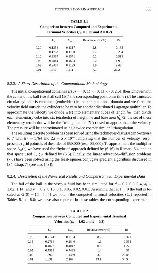
TABLE 8.1
Comparison between Computed and Experimental
Terminal Velocities (ρs = 1.02 andd = 0.2)
ν Uc Uexp Relative error (%) Re
0.20 0.1354 0.1317 2.8 0.1350.15 0.1762 0.1750 0.7 0.2340.10 0.2567 0.2571 0.2 0.5130.05 0.4844 0.4603 5.2 1.930.02 0.9480 0.9129 3.8 9.480.01 1.310 1.411 7.1 26.2
8.2.3. A Short Description of the Computational Methodology
The initial computational domain isÄ(0) = (0, 1)× (0, 1)× (0, 2.5); then it moves withthe center of the ball (we shall callÄ(t) the corresponding position at timet). The truncatedcircular cylinder is contained (embedded) in the computational domain and we force thevelocity field outside the cylinder to be zero by another distributed Lagrange multiplier. Toapproximate the velocity we divideÄ(t) into elementary cubes of lengthhÄ, then divideeach elementary cube into six tetrahedra of heighthÄ and base areah2
Ä/2; the set of theseelementary tetrahedra will be the “triangulation”Th(t) used to approximate the velocity.The pressure will be approximated using a twice coarser similar “triangulation.”
The resulting discrete problem has been solved using the techniques discussed in Section 4to 7 with hÄ = 1/64 and1t = 5× 10⁻⁴, implying that the number of velocity (resp.,pressure) grid points is of the order of 650,000 (resp. 82,000). To approximate the multiplierspace3h(t) we have used the “hybrid” approach defined by (6.16) in Remark 6.4, and onthat space used〈., .〉 jh defined by (6.6). Finally, the linear advection–diffusion problems(7.6) have been solved using the least-squares/conjugate gradient algorithms discussed in[34, Chap. 7] (see also [43]).
8.2.4. Description of the Numerical Results and Comparison with Experimental Data
The fall of the ball in the viscous fluid has been simulated ford = 0.2, 0.3, 0.4, ρs =1.02, 1.14, andν = 0.2, 0.15, 0.1, 0.05, 0.02, 0.01. Assuming that att = 0 the ball is lo-cated atG(0) = {.5, .5, .5} we obtain the computed terminal velocities(Uc) reported inTables 8.1 to 8.6; we have also reported in these tables the corresponding experimental
TABLE 8.2
Comparison between Computed and Experimental Terminal
Velocities (ρs = 1.02 andd = 0.3)
ν Uc Uexp Relative error (%) Re
0.20 0.2144 0.2164 0.9 0.3210.15 0.2794 0.2840 1.6 0.5580.10 0.4072 0.4047 0.6 1.220.05 0.7599 0.7493 1.4 4.560.02 1.392 1.4359 3.0 20.850.01 1.831 2.107 13.1 54.9

386 GLOWINSKI ET AL.
TABLE 8.3
Comparison between Computed and Experimental
Terminal Velocities (ρs = 1.02 andd = 0.4)
ν Uc Uexp Relative error (%) Re
0.20 0.2536 0.2487 2 0.5070.15 0.3299 0.3362 1.9 0.880.10 0.4799 0.4977 3.6 1.920.05 0.8930 0.8600 3.8 7.140.02 1.625 1.695 4.2 32.50.01 2.098 2.422 13.4 84
TABLE 8.4
Comparison between Computed and Experimental
Terminal Velocities (ρs = 1.14 andd = 0.2)
ν Uc Uexp Relative error (%) Re
0.20 0.9367 0.8707 7.6 0.9370.15 1.203 1.102 9.2 1.600.10 1.672 1.552 7.7 3.340.05 2.617 2.489 5.1 10.50.02 3.812 4.334 12 38.1
TABLE 8.5
Comparison between Computed and Experimental
Terminal Velocities (ρs = 1.14 andd = 0.3)
ν Uc Uexp Relative error (%) Re
0.20 1.478 1.401 5.5 2.220.15 1.888 1.786 5.7 3.780.10 2.574 2.426 6.1 7.710.05 3.823 3.972 3.7 22.90.02 5.216 6.283 17 78.3
TABLE 8.6
Comparison between Computed and Experimental
Terminal Velocities (ρs = 1.14 andd = 0.4)
ν Uc Uexp Relative error (%) Re
0.20 1.746 1.673 4.3 3.490.15 2.226 2.057 8.2 5.930.10 3.031 2.868 5.7 12.10.05 4.448 4.573 2.7 35.60.02 5.892 6.946 15.2 118

FICTITIOUS DOMAIN APPROACH 387
terminal velocities (Uexp) (obtained from [42]), the associated relative errors, and the cor-responding Reynolds number (based on the formula Re= Ucd/ν).
It is our opinion that the agreement between computed and experimental terminal veloci-ties is quite good, particularly if one takes into consideration that the experimental terminalvelocities taken from Ref. [42] are obtained, in fact, by multiplying the terminal velocitiesof a ball falling in an unbounded flow region (in practice a region very large compared tothe size of the ball) by a wall correction factor. This explains the large number of digitsin the experimental data and suggests, also, that these data contain other errors than thosedue to measurement. Actually, the large discrepancies observed forν = 0.01, ρs = 1.02andν = 0.02, ρs = 1.14 are very likely caused by the fact that when the falling velocitybecomes sufficiently large asymmetry breakingtakes place, and the ball “leaves” the axisof the cylinder and falls along a spiraling trajectory. For more details about the test casediscussed in this section and further comparisons with experimental data see Ref. [44].
8.3. Numerical Simulation of the Sedimentation of a Circular Disk
8.3.1. Description of the Test Problem
The objective of this test problem is to simulate the fall of a rigid circular disk in abounded cavityÄ filled with an incompressible Newtonian viscous fluid. Simulating theimpact of the cylinder with the bottom boundary of the cavity is part of the computationalexperiment.
8.3.2. On the Computational Methodology
The computational techniques used for the simulations are those discussed in Sections 4to 7. To construct the triangulationsTh used to approximate the velocity, we have firstdivided the cavityÄ into elementary squares of lengthhÄ and then each square into twotriangles as shown in Fig. 8.1.
We proceed similarly to construct the (twice coarser) pressure grid. The multiplier space3(t) and the pairing〈., .〉 have been approximated as in Section 8.2.3. Concerning now thetreatment of the advection–diffusion two approaches have been implemented, namely the
FIG. 8.1. Division of an elementary square.

388 GLOWINSKI ET AL.
global approach where advection and diffusion are treated at once as in Section 8.2.3 andthe approach advocated in Remark 7.2 where a wave-like equation method is used to treatthe advection after decoupling from diffusion via an additional fractional step in scheme(7.4)–(7.19) (see Remark 7.2 for details). Actually, we have used these two approaches inorder to cross-validate our computational methods.
8.3.3. On the Geometry, Initial and Boundary Conditions, and Other Parameters
• The computational domain isÄ = (0, 2)× (0, 6).• The diameter of the disk isd = 0.25.• The centerG of the disk is located at{1, 4} at timet = 0.• The fluid and the disk are initially at rest, i.e.,u(0)(=u0) = 0, G(0) = ω(0) = 0.• The fluid velocity is0, ∀t ≥ 0, on the boundary ofÄ.• The fluid density isρf = 1.• The disk densityρs is either 1.25 or 1.5.• The fluid viscosityν is either 0.1 or 0.01.• The velocity mesh sizehÄ is either 1/192 or 1/256 or 1/384; the pressure mesh
size ishp = 2hÄ.• The time discretization step1t is either 10−3 or 7.5× 10⁻⁴ or 5× 10⁻⁴.• The parameterε used in the collision model is of the order of 10−5.
From the above characteristics we can see that we have (approximately) 440,000, 786,000,and 1.77× 10⁶ (resp., 110,000, 196,000, and 442,000) vertices for the three velocity (resp.,pressure) triangulations used for the simulations.
8.3.4. Description of the Numerical Results
In Fig. 8.2 we have visualized the flow and the particle position att = 0.3 for ρs = 1.25and ν = 0.1. The figures associated tohÄ = 1/192, 1t = 10−3 are practically undis-cernible of those obtained withhÄ = 1/256, 1t = 7.5× 10⁻⁴, andhÄ = 1/384, 1t =5× 10⁻⁴. Similarly, the figures associated to the least-squares/conjugate gradient treat-ment of the advection–diffusion and those obtained from the wave-like equation treatmentof the advection are essentially identical. Further results and comparisons are shown inFigs. 8.3 to 8.5.
The above figures show that, in practice, the cylinder quickly reaches a uniform fallingvelocity until it hits the bottom of the cavity. A careful examination of Fig. 8.3 showsthat a symmetry breaking of small amplitude is taking place with the disk moving slightlyon the right, away from the vertical symmetry axis of the cavity. Figure 8.5 shows thatthe rotational component of the kinetic energy is small compared to the translational one.The maximal computed disk Reynolds numbers are 17.27 forhÄ = 1/192, 1t = 10−3 and17.31 forhÄ = 1/256, 1t = 7.5× 10⁻³.
The results obtained using the wave-like equation approach to treat advection (oncedecoupled from diffusion) are very close to those which have been reported above. Anevidence of this very good agreement is provided by Fig. 8.6 where we have compared thekinetic energies obtained by both approaches.
Another evidence of the good agreement between both approaches is that the maximumdisk Reynolds numbers obtained via the wave-like equation method are 17.44 forhÄ =1/192, 1t = 10−3 and 17.51 forhÄ = 1/256, 1t = 7.5× 10⁻⁴, to be compared to 17.27and 17.31.
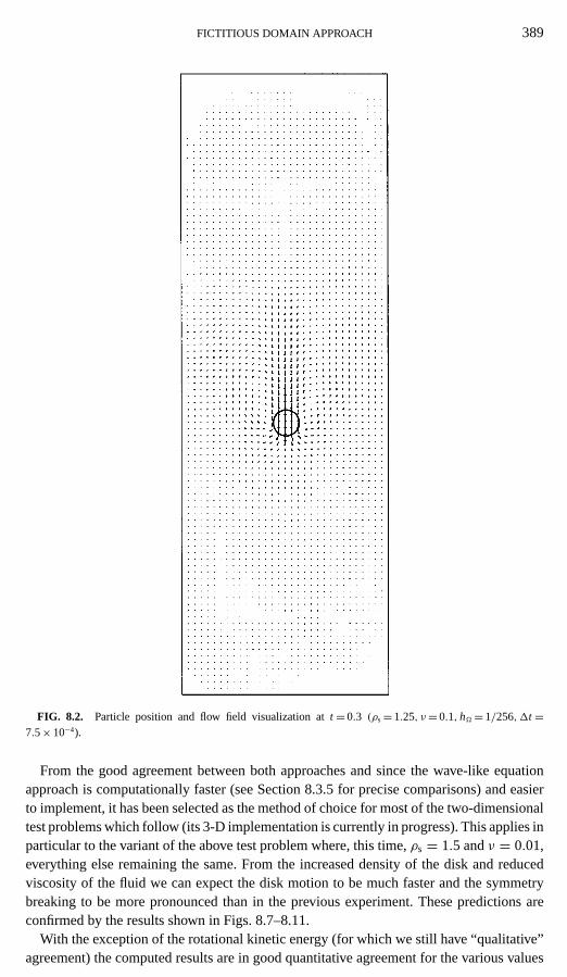
FICTITIOUS DOMAIN APPROACH 389
FIG. 8.2. Particle position and flow field visualization att = 0.3 (ρs= 1.25, ν= 0.1, hÄ= 1/256,1t =7.5× 10⁻⁴).
From the good agreement between both approaches and since the wave-like equationapproach is computationally faster (see Section 8.3.5 for precise comparisons) and easierto implement, it has been selected as the method of choice for most of the two-dimensionaltest problems which follow (its 3-D implementation is currently in progress). This applies inparticular to the variant of the above test problem where, this time,ρs = 1.5 andν = 0.01,everything else remaining the same. From the increased density of the disk and reducedviscosity of the fluid we can expect the disk motion to be much faster and the symmetrybreaking to be more pronounced than in the previous experiment. These predictions areconfirmed by the results shown in Figs. 8.7–8.11.
With the exception of the rotational kinetic energy (for which we still have “qualitative”agreement) the computed results are in good quantitative agreement for the various values

390 GLOWINSKI ET AL.
FIG. 8.3. Histories of thex-coordinate (left) andy-coordinate (right) of the center of the disk forρs= 1.25andν= 0.1(hÄ= 1/192 and1t = 10−3, solid lines;hÄ= 1/256 and1t = 7.5× 10⁻⁴, dashed–dotted lines). Least-squares/conjugate gradient treatment of advection–diffusion.
FIG. 8.4. Histories of thex-component (left) andy-component (right) of the translation velocity of the diskfor ρs= 1.25 andν= 0.1(hÄ= 1/192 and1t = 10−3, solid lines;hÄ= 1/256 and1t = 7.5× 10⁻⁴, dashed–dottedlines). Least-squares/conjugate gradient treatment of advection–diffusion.
FIG. 8.5. Histories of translational (left) and rotational (right) kinetic energies of the disk forρs= 1.25 andν= 0.1(hÄ= 1/192 and1t = 10−3, solid lines;hÄ= 1/256 and1t = 7.5× 10⁻⁴, dashed–dotted lines). Least-squares/conjugate gradient treatment of advection–diffusion.
FICTITIOUS DOMAIN APPROACH 391
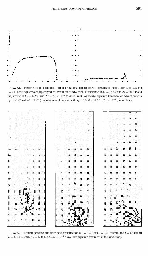
FIG. 8.6. Histories of translational (left) and rotational (right) kinetic energies of the disk forρs= 1.25 andν= 0.1. Least-squares/conjugate gradient treatment of advection–diffusion withhÄ= 1/192 and1t = 10−3 (solidline) and withhÄ= 1/256 and1t = 7.5× 10⁻⁴ (dashed line). Wave-like equation treatment of advection withhÄ= 1/192 and1t = 10−3 (dashed–dotted line) and withhÄ= 1/256 and1t = 7.5× 10⁻⁴ (dotted line).
FIG. 8.7. Particle position and flow field visualization att = 0.3 (left), t = 0.4 (center), andt = 0.5 (right)(ρs= 1.5, ν= 0.01,hÄ= 1/384,1t = 5× 10⁻⁴; wave-like equation treatment of the advection).

392 GLOWINSKI ET AL.
FIG. 8.8. Histories of thex-coordinate (left) andy-coordinate (right) of the center of the disk forρs= 1.5andν= 0.01 (hÄ= 1/256 and1t = 7.5× 10⁻⁴, solid lines;hÄ= 1/384 and1t = 5× 10⁻⁴, dashed–dotted lines;wave-like equation treatment of the advection).
FIG. 8.9. Histories of thex-coordinate (left) andy-coordinate (right) of the translation velocity of the diskfor ρs= 1.5 andν= 0.01(hÄ= 1/256 and1t = 7.5× 10⁻⁴, solid lines;hÄ= 1/384 and1t = 5× 10⁻⁴, dashed–dotted lines; wave-like equation treatment of the advection).
FIG. 8.10. History of the angular velocity of the disk forρs= 1.5 andν= 0.01 (hÄ= 1/256 and1t =7.5× 10⁻⁴, solid line;hÄ= 1/384 and1t = 5× 10⁻⁴, dashed–dotted line; wave-like equation treatment of theadvection).

FICTITIOUS DOMAIN APPROACH 393
FIG. 8.11. Histories of the translational (left) and rotational (right) kinetic energies of the disk forρs= 1.5andν= 0.01 (hÄ= 1/256 and1t = 7.5× 10⁻⁴, solid lines;hÄ= 1/384 and1t = 5× 10⁻⁴, dashed–dotted lines;wave-like equation treatment of the advection).
of hÄ and1t . In particular, the maximum computed disk Reynolds numbers are 438.6for hÄ = 1/192 and1t = 10−3, 450.7 forhÄ = 1/256 and1t = 7.5× 10⁻⁴, and 466 forhÄ = 1/384 and1t = 5× 10⁻⁴; this is quite good agreement if one considers that oneis dealing with a highly nonlinear phenomenon involving symmetry breaking. Actually,the above figures show that the symmetry breaking weakens ash and1t decrease. Thisis not surprising since the above symmetry breaking is triggered by the (non-symmetric)perturbations associated to our numerical methods (our triangulations, for example, arenot symmetric with respect to the cavity axis (i.e., the linex1 = 3)); ash decreases thequality of the approximation increases implying that the level of perturbation decreases,leading to symmetry breakings of smaller amplitude. Let us observe that forhÄ = 1/384the velocity (resp., pressure) triangulation has approximately 1.77× 10⁶ (resp., 442,000)vertices, respectable numbers indeed.
8.3.5. Further Details on Implementation
Let us provide some further information concerning the computer implementation ofthe methods discussed in Sections 3 to 7, when applied to the test problem described inSections 8.3.1 and 8.3.3. Without going into excruciating detail, let us say that:
• We have takenε ranging from 5× 10⁻⁵ to 5× 10⁻⁶ in the collision model associatedto relation (5.2). The parameterρ in (5.2) (the thickness of the safety zone) has been takenof the order of 2.5hÄ.• The number of conjugate gradient iterations necessary to force the discrete incom-
pressibility is of the order of 12.• If the least-squares/conjugate gradient methodology advocated in [37] and [43] is
used to treat the advection–diffusion it requires two (preconditioned) iterations at most.• If one uses the wave-like equation approach to treat the advection the number of
sub-time steps used to integrate the wave-like equation (7.26) is of the order of five.• The number of iterations necessary to force the rigidity inside the disk varies from
70 to 100 (it increases with the maximal Reynolds number). This may seem quite large, butthings have to be put in perspective for the following reasons:
(i) The dimension of the discrete multiplier space3h is small compared to thedimensions of the velocity spaceVh and pressure spacePh. We have indeed

394 GLOWINSKI ET AL.
TABLE 8.7
CPU per Time Step (in Seconds)
ρs ν h 1t Adv. treat. CPU/timestep(s)
1.25 0.1 1/192 10−3 l.s./c.g. 29.71.25 0.1 1/192 10−3 w.-l. eq. 25.61.25 0.1 1/256 7.5× 10⁻⁴ l.s./c.g. 60.81.25 0.1 1/256 7.5× 10⁻⁴ w.-l. eq. 60.61.5 10−2 1/192 10−3 w.-l. eq. 311.5 10−2 1/256 7.5× 10⁻⁴ w.-l. eq. 54.81.5 10−2 1/384 5× 10⁻⁴ w.-l. eq. 140.8
dimVh ' 880,000, dimPh ' 110,000, and dim3h ' 3,700 if h = 1/192,dimVh ' 1.57× 10⁶, dimPh ' 196,000, and dim3h ' 6,400 if h = 1/256,dimVh ' 3.54× 10⁶, dimPh ' 42,000, and dim3h ' 14,600 if h = 1/384.
(ii) The problems of type (7.20) encountered in this application have been solvedby a diagonally preconditioned conjugate gradient algorithm implying that each iterationis quite inexpensive.
From the above reasons, most of the CPU time is spent in solving the Navier–Stokes equa-tions. Of course for those situations with many particles, where the ratio solid volume/fluidvolume is of order 1 it may be worthwhile to precondition the conjugate gradient algorithm,used to compute the multipliers, by the symmetric and positive definite matrices associatedto the scalar products (4.16) or (4.17) restricted to3 jh .
• The discrete Poisson problems encountered in computing the discrete pressure andforcing the discrete incompressibility condition “take place” on a regular grid; we cantherefore usefast Poisson Solversbased oncyclic reductionto solve these problems (see,e.g., Ref. [45] for a discussion of cyclic reduction methods). Similarly, the elliptic problemsencountered when treating diffusion (with or without advection) can be solved by fast directsolvers based on cyclic reduction.• The wave-like equation-based methodology (w.-l. eq.) seems to be 20% faster than
the one based on the least-squares/conjugate gradient treatment (l.s./c.g.) of advection–diffusion; it is also easier to implement.• The computational times per time step on a one-processor DEC Alpha 500-au work-
station are given in Table 8.7 (where the notation is self-explanatory). These figures can besubstantially reduced via parallelization since the good potential for parallelization of thefictitious domain methods has not been taken advantage of in these simulations (see, e.g.,ref. [46] for the parallelization of the fictitious domain methods discussed in this article).
8.4. Numerical Simulation of the Motion and Interaction of Two Circular DisksSedimenting in an Incompressible Newtonian Viscous Fluid
8.4.1. Description of the Test Problem
The objective of this test problem is to simulate the motion and the interaction of twoidentical rigid circular disks sedimenting in a vertical channel. The two disks are initially atrest on the axis of the channel, the distance between their centers being one disk diameter.

FICTITIOUS DOMAIN APPROACH 395
We expect the simulations to reproduce the well documenteddrafting, kissing, and tumblingphenomenon; this phenomenon has been observed in laboratory experiments and also viasimulations based on computational methods different of the ones discussed in this article(see, for example, [47, 48], and the references therein).
The computational methods used for this test problem are those already employed forthe test problems of Section 8.3.
8.4.2. On the Geometry, Initial and Boundary Conditions, and Other Parameters
• The computational domain at timet = 0 isÄ(0) = (0, 2)× (0, 6) and is movingwith the disks.• The diameter of the disks isd = 0.25.• The initial positions of the disk centers are{1, 4.5} and{1, 5}.• The fluid and the disks are initially at rest.• The fluid velocity is0, ∀t ≥ 0, on the boundary of the channel.• The fluid density isρf = 1.• The disk density isρs = 1.5.• The fluid viscosity isν = 0.01.• The discretization parameters are{hÄ,1t} = {1/192, 10−3}, {1/256, 7.5× 10⁻⁴},
{1/384, 5× 10⁻⁴}.• The collision parameter isε = 5× 10⁻⁶.• The safety zone thicknessρ in the collision model ranges from 2hÄ to 4hÄ.
8.4.3. Description of the Numerical Results
The results shown below have been obtained using the wave-like equation approach ofSection 7.3, Remark 7.2, to treat the advection.
The drafting, kissing, and tumbling phenomenon mentioned above is clearly observed inFig. 8.12. The accepted explanation of this phenomenon is as follows:
The lower disk, when falling, creates a pressure drop in its wake. This implies that—if initially close enough—the upper disk encounters less resistance from the fluid thanthe lower one and falls faster. Falling faster, the upper disk touches (or almost touches)the lower one. Once in contact (or quasi-contact), the two disks act as an elongated bodyfalling in an incompressible viscous fluid. As is well known, elongated bodies falling suf-ficiently fast in a Newtonian incompressible viscous fluid have a tendency to rotate sothat their broad sides become perpendicular to the flow direction. Indeed rotation takesplace, as seen is Fig. 8.12 att = 0.2, but the two-disks assemblage is unstable and thetwo disks separate. The maximum computeddisk Reynolds numberis 664 (resp., 680 and689) for {hÄ,1t} = {1/192, 10−3} (resp.,{1/256, 7.5× 10⁻⁴} and {1/384, 5× 10⁻⁴}).The computedminimal distancebetween the two disks is 1.26hÄ, 1.03hÄ, and 2.1hÄfor {hÄ,1t} = {1/192, 10−3}, {1/256, 7.5× 10⁻⁴} and {1/394, 5× 10⁻⁴}; it occurs att = 0.157, 0.161, and 0.163, respectively. Considering that drafting, kissing, and tum-bling is a violent phenomenon (see Fig. 8.14 for evidence of this violence) the agree-ment between the computed results for the various values ofhÄ and1t is quite good.Calculations done withρs = 1.25 confirm the above results; actually, the agreement iseven better since the disk motions and fluid flow are slower due to the smaller value ofρs− ρf .

396 GLOWINSKI ET AL.
FIG. 8.12. Disks positions and flow field visualization att = 0.15, 0.2, and 0.3 (ρs= 1.5, ν= 10−2, hÄ=1/384,1t = 5× 10⁻⁴). Wave-like equation treatment of the advection.
The various observations and comments done in Section 8.3.3 (for the sedimentation ofone disk) still apply to the present test problem (see Figs. 8.13–8.15). Actually, the costsand numbers of iterations associated to the solution of the various subproblems are close,although the two-disk simulation is a bit more expensive than the one-disk one, since it
FIG. 8.13. Histories of thex-coordinate (left) andy-coordinate (right) of the centers of the disks forρs=1.5 andν= 10−2 (hÄ= 1/256,1t = 7.5× 10⁻⁴, solid lines;hÄ= 1/384,1t = 5× 10⁻⁴, dashed–dotted lines).Wave-like equation treatment of the advection.

FICTITIOUS DOMAIN APPROACH 397
FIG. 8.14. Histories of thex-coordinate (left) andy-coordinate (right) of the translational velocity of thedisks for ρs= 1.5 and ν= 10−2 (hÄ= 1/256, 1t = 7.5× 10⁻⁴, solid lines; andhÄ= 1/384, 1t = 5× 10⁻⁴,dashed–dotted lines). Wave-like equation treatment of the advection.
leads to higher Reynolds numbers for the same values ofρs, ρf , andν. For example, theCPU times per time-step on the same DEC Alpha 500-au workstation are 44, 79, and 200 sfor {hÄ,1t} = {1/192, 10−3}, {1/256, 7.5× 10⁻⁴}, and{1/384, 5× 10⁻⁴}, respectively(compared to 31, 55, and 141 s for the one-disk problem).
8.5. Numerical Simulation of the Motions and Interaction of Two BallsSedimenting in an Incompressible Viscous Fluid
The fourth test problem considered here concerns the simulation of the motions and in-teraction of two sedimenting identical balls in a vertical cylinder with square cross-section.The computational domain isÄ = (0, 1)× (0, 1)× (0, 4). The diameterd of the two ballsis 1/6 and at timet = 0, the centers of the two balls are located on the axis of the cylinder at{0.5, 0.5, 3.5}and{0.5, 0.5, 3.16}. The initial translational and angular velocities of the ballsare zero. The density of the fluid isρf = 1.0 and the density of the balls isρs = 1.14. The vis-cosity of the fluid isνf = 0.01. The initial condition for the fluid flow isu(0)(=u0) = 0whilethe boundary condition isu(t) = 0 on the boundary of the cylinder,∀t ≥ 0. The simulation
FIG. 8.15. Histories of the angular velocities of the disks (left) and of their distance (right) forρs= 1.5 andν= 10−2 (hÄ= 1/256,1t = 7.5× 10⁻⁴, solid lines;hÄ= 1/384,1t = 5× 10⁻⁴, dashed–dotted lines). Wave-likeequation treatment of the advection.
398 GLOWINSKI ET AL.
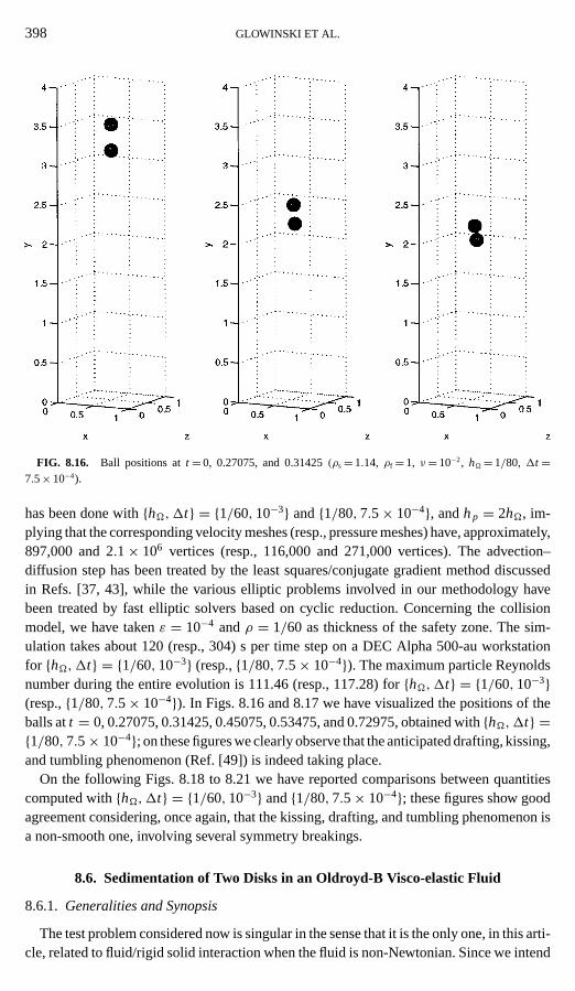
FIG. 8.16. Ball positions att = 0, 0.27075, and 0.31425(ρs= 1.14, ρf = 1, ν= 10−2, hÄ= 1/80, 1t =7.5× 10⁻⁴).
has been done with{hÄ,1t} = {1/60, 10−3} and{1/80, 7.5× 10⁻⁴}, andhp = 2hÄ, im-plying that the corresponding velocity meshes (resp., pressure meshes) have, approximately,897,000 and 2.1× 10⁶ vertices (resp., 116,000 and 271,000 vertices). The advection–diffusion step has been treated by the least squares/conjugate gradient method discussedin Refs. [37, 43], while the various elliptic problems involved in our methodology havebeen treated by fast elliptic solvers based on cyclic reduction. Concerning the collisionmodel, we have takenε = 10−4 andρ = 1/60 as thickness of the safety zone. The sim-ulation takes about 120 (resp., 304) s per time step on a DEC Alpha 500-au workstationfor {hÄ,1t} = {1/60, 10−3} (resp.,{1/80, 7.5× 10⁻⁴}). The maximum particle Reynoldsnumber during the entire evolution is 111.46 (resp., 117.28) for{hÄ,1t} = {1/60, 10−3}(resp.,{1/80, 7.5× 10⁻⁴}). In Figs. 8.16 and 8.17 we have visualized the positions of theballs att = 0, 0.27075, 0.31425, 0.45075, 0.53475, and 0.72975, obtained with{hÄ,1t} ={1/80, 7.5× 10⁻⁴}; on these figures we clearly observe that the anticipated drafting, kissing,and tumbling phenomenon (Ref. [49]) is indeed taking place.
On the following Figs. 8.18 to 8.21 we have reported comparisons between quantitiescomputed with{hÄ,1t} = {1/60, 10−3} and{1/80, 7.5× 10⁻⁴}; these figures show goodagreement considering, once again, that the kissing, drafting, and tumbling phenomenon isa non-smooth one, involving several symmetry breakings.
8.6. Sedimentation of Two Disks in an Oldroyd-B Visco-elastic Fluid
8.6.1. Generalities and Synopsis
The test problem considered now is singular in the sense that it is the only one, in this arti-cle, related to fluid/rigid solid interaction when the fluid is non-Newtonian. Since we intend

FICTITIOUS DOMAIN APPROACH 399
FIG. 8.17. Ball positions att = 0.45075, 0.53475, and 0.72925(ρs= 1.14, ρf = 1, ν= 10−2, hÄ= 1/80,1t = 7.5× 10⁻⁴).
to publish, in the not too far future, an article specifically dedicated to the direct numericalsimulation of visco-elastic particulate flow, our “visit” to the non-Newtonian realm will berather brief; actually, our main intention is to show some fundamental differences betweenthe behavior of Newtonian and visco-elastic fluids when sedimentation is concerned. Weconsider thus the simulation of two rigid disks sedimenting in a two-dimensional cavityfilled with anOldroyd-B visco-elastic fluid. The equations describing the rigid body motionsare as in Section 2; concerning the flow model we have to complete Equations (2.1)–(2.4)
FIG. 8.18. Histories of thex-component of the ball centers (left) and of thex-component of the ball translationvelocity (right) forρs= 1.14,ρf = 1, andν= 10−2 (hÄ= 1/60,1t = 10−3, solid lines;hÄ= 1/80,1t = 7.5× 10⁻⁴,dashed–dotted lines).

400 GLOWINSKI ET AL.
FIG. 8.19. Histories of they-component of the ball centers (left) and of they-component of the ball translationvelocity (right) forρs= 1.14,ρf = 1, andν= 10−2 (hÄ= 1/60,1t = 10−3, solid lines;hÄ= 1/80,1t = 7.5× 10⁻⁴,dashed–dotted lines).
with (see [45, pp. 185–187])
τ + λ1∇τ = 2η(τ + λ2
∇D(u)), (8.1)
where in (8.1):
• A d × d tensorA being given,∇A denotes the upper convected derivative ofA,
defined by
∇A = ∂A
∂t+ (u · ∇)A − (∇u)A − A(∇u)t ; (8.2)
• λ1 is the relaxation time;• λ2 is the retardation time;• η = (λ1/λ2)νf , whereνf is the fluid viscosity,• D(u) = (∇u+∇ut )/2.
FIG. 8.20. Histories of thez-component of the ball centers (left) and of thez-component of the ball translationvelocity (right) forρs= 1.14,ρf = 1, andν= 10−2 (hÄ= 1/60,1t = 10−3, solid lines;hÄ= 1/80,1t = 7.5× 10⁻⁴,dashed–dotted lines).

FICTITIOUS DOMAIN APPROACH 401
FIG. 8.21. History of the distance between the two balls forρs= 1.14, ρf = 1, andν= 10−2 (hÄ= 1/60,1t = 10−3, solid lines;hÄ= 1/80,1t = 7.5× 10⁻⁴, dashed–dotted lines).
Generalizing the splitting scheme (7.4)–(7.19) to accommodate the additional relation (8.1)is not difficult; we can, in particular, use the wave-like equation approach discussed inSection 7.3 to treat the advection term∂τ/∂t + (u · ∇)τ occurring in (8.1) (from (8.2))and apply a time stepping method to the resulting problem (this approach was followed inRef. [39]).
Remark 8.1. Detailed discussions on the modeling and simulation of theflow of visco-elastic liquidscan be found in Refs. [50, 51]; see also the many references therein.
8.6.2. Formulation of the Test Problem and Numerical Results
As already mentioned, this fifth test problem is concerned with the direct simulation ofthe sedimentation of two rigid disks in a two-dimensional cavity filled with an Oldroyd-Bvisco-elastic fluid. The computational domain isÄ = (0, 2)× (0, 6). The initial conditionfor the fluid velocity field isu(0)(=u0) = 0. The boundary condition for the velocity isu(t) = 0 on 0, ∀t ≥ 0. The density of the fluid isρf = 1 and the viscosity isνf = 0.25.The relaxation time isλ1 = 1.4, while the retardation time isλ2 = 0.7. The diameter ofthe disks isd = 0.25, while their density isρs = 1.01. The initial translation and angularvelocities of the disks are zeros. At timet = 0, the centers of the two disks are locatedon the vertical symmetry axis of the cavity at{1, 5.25} and {1, 4.75}. In the simulation,the mesh size for the velocity fieldhÄ = 1/128; it is hp = 2hÄ = 1/64 for the pressureandhτ = hÄ = 1/128 for the stress tensorτ . The time step is1t = 10−3. We let the twodisks fall in the cavity. Before touching the bottom, we can see in Fig. 8.22 the fundamentalfeatures of a pair of identical disks sedimenting in an Oldroyd-B viscoelastic fluid, namelya drafting, kissing, and chaining phenomenon (see [52] for more details). The averagedterminal velocity is 0.29 in this simulation, implying that the corresponding
• Deborah numberis De= 1.624• Reynolds numberis Re= 0.29• Visco-elastic Mach numberis M = 0.686• Elasticity numberis E = 5.6

402 GLOWINSKI ET AL.
FIG. 8.22. Sedimentation and chaining of two disks in an Oldroyd-B viscoelastic fluid att = 3, 11, 15, 18,22.5, and 27 (from left to right and from top to bottom).

FICTITIOUS DOMAIN APPROACH 403
(see, e.g., Ref. [51] for a precise definition of De,M , andE). The simulation has been doneusing the wave-like equation approach, discussed in Section 7.3, to treat the advection ofuandτ .
8.7. Direct Numerical Simulation of Incompressible ViscousFlow around Moving Airfoils
8.7.1. Motivation and Synopsis
The rigid bodies considered so far have been circular disks or spherical balls. Anothersalient feature of the previous test problems and simulations has been that the rotationalkinetic energy was always small compared to the translational kinetic energy. The maingoals of the following two test problems are:
(i) To show that the computational methods discussed in Sections 4 to 7 apply (at leastin 2-D) to rigid bodies of shape more complicated than disks and balls.
(ii) To show that the above methods apply when the rotational kinetic energy is com-parable, or even larger, to the translational one and still can bring accurate results.
The following test problems concern flow around one or several NACA0012 airfoils.
8.7.2. Flow around a NACA0012 Airfoil with Fixed Center of Mass
We consider here an incompressible viscous flow around a NACA0012 airfoil that hasa fixedcenter of mass and isfree to rotatedue to hydrodynamical forces; the surroundingregionÄ is the rectangle (−4, 16)× (−2, 2). The characteristic length, namely the airfoillength, is 1.009 and the fixed center of mass of the airfoil is at (0.42, 0). Initial angularvelocity and incident angle are zero. The density of the fluid isρf = 1 and the density ofthe airfoil isρs = 1.1. The viscosity of the fluid isνf = 10−2. The initial condition for thefluid flow is u(0)(=u0) = 0 and the boundary datag0 is given by
g0(x, t) ={
0 if x2 = −2 or 2,(1− e−50t )
(10
)if x1 = −4 or 16,
for t ≥ 0. Hence the Reynolds number is about 101 with respect to the length of the airfoiland the maximum inflow speed. For this test problem we have chosen two sets{hÄ,1t}of discretization parameters, namely{1/64, 1.5× 10⁻³} and{1/96, 10−3}, to validate thesimulation results; the mesh size for pressure is, again,hp = 2hÄ. We have thus, approxi-mately, 330,00 and 740,000 velocity vertices for the triangulations used to approximate thevelocity.
To enforce the rigid body motion inside the airfoil at each time step, using the multiplierspace defined by (6.16), we have taken all the grid points from the velocity mesh containedin the airfoil at that time completed by a selected set of points belonging to the boundary ofthe airfoil (and containing the trailing edge; see Fig. 8.23) and then used as scalar productover3h(t) the one defined by (6.6).
For these rotating airfoil simulations, we have used the previously mentioned leastsquares/conjugate gradient technique to solve the advection-diffusion subproblems. TheNACA0012 airfoil is fixed up tot = 1. A steady flow around it is obtained. Aftert = 1,we allow the NACA0012 airfoil to rotate freely. In Fig. 8.24, we observe that the histories

404 GLOWINSKI ET AL.
FIG. 8.23. Part of the velocity mesh and example of mesh points used in (6.16) to enforce the rigid bodymotion inside the NACA0012 airfoil.
corresponding to the two sets{hÄ,1t} are in very good agreement. The airfoil intendsto keep its broadside perpendicular to the in-flow direction which is a stable position fornon-circular particles settling in a channel at small Reynolds numbers (cf. Ref. [53]) and itquickly reaches a periodic motion.
The CPU/time step is 53 s (resp., 107 s if{hÄ,1t} = {1/64, 1.5× 10⁻³} (resp.,{1/96,10−3}) on one node of an IBM SP2. The same methodology has been (successfully)applied to the more challenging case whereνf = 1.25× 10⁻³ (i.e., Re= 807) the otherdata and parameters staying the same. The corresponding results are discussed in [6,Sect. 6].
Remark 8.2. For the test case discussed here the fact that we used a fine uniform meshmay appear as a drawback. Actually, this test problem was considered for validation purposesand also to show that our methodology can handle non-circular bodies. Also, when simulat-ing the flow of mixtures with over 100 particles highly dispersed in the flow region (see thetest problems in Sections 8.8 and 8.9), which is the main goal of the distributed Lagrangemultiplier method discussed here, using a fine uniform mesh everywhere is not a drawback

FICTITIOUS DOMAIN APPROACH 405
FIG. 8.24. Histories of the angle (hÄ= 1/64,1t = 1.5× 10⁻³, dotted line;hÄ= 1/96,1t = 10−3, dashed–dotted line) and of the angular velocity (hÄ= 1/64,1t = 1.5× 10⁻³, dashed line;hÄ= 1/96,1t = 10−3, solidline). The measures are in rad and rad/s.
FIG. 8.25. Flow visualization att = 1.

406 GLOWINSKI ET AL.
anymore (particularly for a flow where the ratiosolid volume/fluid volumeis of the order ofone or more).
Of course—as in [54]—one can combine locally adapted mesh with boundary Lagrangemultiplier in order to avoid using fine mesh everywhere. One can also use unstructuredmeshes and force the rigid body motion by collocation like the one done in [22].
Remark 8.3. For the above test problem, we have imposedu = 0 on the top and bottomboundaries ofÄ. Actually, with the methodology discussed in this article, there would
FIG. 8.26. Flow visualization (top) and vorticity density (bottom) att = 1.3.

FICTITIOUS DOMAIN APPROACH 407
have been no problem imposingu = u∞(6=0) on the inflow, top and bottom boundariesof Ä andνf(∂u/∂n)− np = 0 (or σn = 0) on the outflow boundary. We can justify theboundary conditions used here by the fact that the experimental results concerning flowaround cylinders are obtained by putting the cylinders in channels where they are fixed orfree to rotate, the boundary conditions on the boundary of the channel being close to thoseused in this article.
Remark 8.4. Using the parallelization techniques discussed in [46], the computationaltimes given above have been divided by factors of the order of 10 (see [46] for details).
FIG. 8.27. Flow visualization (top) and vorticity density (bottom) att = 1.5.

408 GLOWINSKI ET AL.
8.7.3. Simulation of a Two-Dimensional Multi-store Separation Phenomenon
The main goal of this test problem is the direct numerical simulation of a multi-storeseparation phenomenon in two-dimensions. A more precise description of the problem isas follows: several bodies, rigidly attached up to some timet∗, are located in a space regioncontaining an incompressibly Newtonian viscous fluid; at timet = t∗, some of the bodies arereleased and are going to fall under the effect of gravity. Our goal is to simulate the motionof the various bodies and the flow they induce when moving down. The computationaldomain isÄ = (−4, 12.047)× (−2, 2). The boundary conditions verified byu(t) on the
FIG. 8.28. Flow visualization (top) and vorticity density (bottom) att = 1.75.
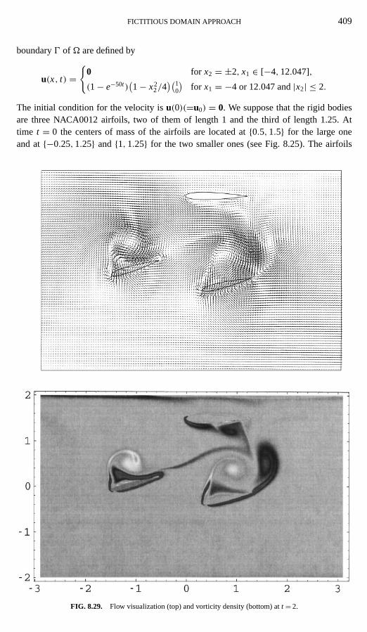
FICTITIOUS DOMAIN APPROACH 409
boundary0 of Ä are defined by
u(x, t) ={
0 for x2 = ±2, x1 ∈ [−4, 12.047],
(1− e−50t )(1− x2
2/4)(1
0
)for x1 = −4 or 12.047 and|x2| ≤ 2.
The initial condition for the velocity isu(0)(=u0) = 0. We suppose that the rigid bodiesare three NACA0012 airfoils, two of them of length 1 and the third of length 1.25. Attime t = 0 the centers of mass of the airfoils are located at{0.5, 1.5} for the large oneand at{−0.25, 1.25} and {1, 1.25} for the two smaller ones (see Fig. 8.25). The airfoils
FIG. 8.29. Flow visualization (top) and vorticity density (bottom) att = 2.

410 GLOWINSKI ET AL.
are at rest att = 0. The two smaller airfoils are released att = t∗ = 1 and start movingdown under the effect of gravity; the largest one is supposed fixed. The fluid density isρf = 1 while the fluid viscosity isνf = 10−3, implying that the moving airfoils’ Reynoldsnumber is 103. The moving airfoils’ density isρs = 1.1. The methods of Sections 4 to7 have been applied (without collision model) to the simulation of the above separationphenomenon. We have usedhÄ = 2/225 to discretize the velocity,hp = 2hÄ to discretizethe pressure, and1t = 5× 10⁻⁴ for the time discretization. We have thus about 106 velocitygrid points and 250,000 pressure grid points. The advection–diffusion has been treated bya least-squares/conjugate gradient method.
FIG. 8.30. Flow visualization (top) and vorticity density (bottom) att = 2.5.

FICTITIOUS DOMAIN APPROACH 411
In Fig. 8.25 we have visualized the flow att = 1 (just before the release of the two smallairfoils), while in Figs. 8.26 to 8.30 we have visualized the flow velocity and the vorticitydistribution att = 1.3, 1.5, 1.75, 2 and 2.5.
The computational time for this test problem is 51 sec./time step on 4 nodes of an SGIOrigin 2000 parallel computer.
FIG. 8.31. Sedimentation of 6400 particles: positions att = 0, 0.4, 0.5, 0.6 (from left to right and from top tobottom), and visualization of the Rayleigh–Taylor instability.

412 GLOWINSKI ET AL.
8.8. Sedimentation of 6,400 Circular Particles in a Two-Dimensional Cavity:Rayleigh–Taylor Instability for Particulate Flow
8.8.1. Generalities and Synopsis
The test problems discussed in this section, and in the following Section 8.9, differsignificantly from the ones considered so far. The main difference lies with the much larger
FIG. 8.32. Sedimentation of 6400 particles:t = 1.

FICTITIOUS DOMAIN APPROACH 413
numbers of rigid bodies (particles, indeed) that we are going to consider, these numbersbeing over 103. Indeed, these test problems can be viewed as particulate flow problems andwe shall see that the computational methods discussed in Sections 4 to 7 apply to thosemore challenging situations.
FIG. 8.33. Sedimentation of 6400 particles:t = 2.6.

414 GLOWINSKI ET AL.
The specific problem discussed in this section concerns the sedimentation of 6,400 diskssettling down in a rectangular cavity filled with an incompressible Newtonian viscousfluid. In Section 8.9 we shall discuss the fluidization of 1,204 spherical particles in athree-dimensional tube (bed). Since several articles specifically dedicated to the above test
FIG. 8.34. Sedimentation of 6400 particles:t = 3.

FICTITIOUS DOMAIN APPROACH 415
problems are in preparation, their discussion in this review article will be shorter than theone they really deserve.
For a review of the many aspects of particulate flow we refer to [55] (and to the manyreferences therein).
FIG. 8.35. Sedimentation of 6400 particles:t = 5.

416 GLOWINSKI ET AL.
8.8.2. Formulation of the Test Problem and Numerical Results
The test problem that we consider now concerns the simulation of the motion of 6,400sedimenting circular disks in the closed cavityÄ = (0, 8)× (0, 12). The diameterd of thedisks is 1/12 and the position of the disks at timet = 0 is shown in Fig. 8.31. The solid
FIG. 8.36. Sedimentation of 6400 particles:t = 7.

FICTITIOUS DOMAIN APPROACH 417
fraction in this test case is 34.9%. The disks and the fluid are at rest a timet = 0. Thedensity of the fluid isρf = 1 and the density of the disks isρs = 1.1. The viscosity of thefluid is νf = 10−2. The time step is 10−3. The mesh size for the velocity field ishÄ = 1/192(the velocity triangulation has thus about 3.5× 10⁶ vertices) while the pressure mesh sizeis hp = 2hÄ, implying approximately 885,000 vertices for the pressure triangulation. For
FIG. 8.37. Sedimentation of 6400 particles:t = 9.

418 GLOWINSKI ET AL.
this test problem where many particles “move around” a fine mesh is required essentiallyeverywhere. The wave-like equation approach has been chosen to treat the advection, theparameterε occurring in the collision model has been taken equal to 10−6, while for thethicknessρ of the safety zone we have usedρ = 2hÄ. The computational time per time stepis approximately 10 min on a DEC Alpha 500-au workstation, implying that to simulate
FIG. 8.38. Sedimentation of 6400 particles:t = 11.
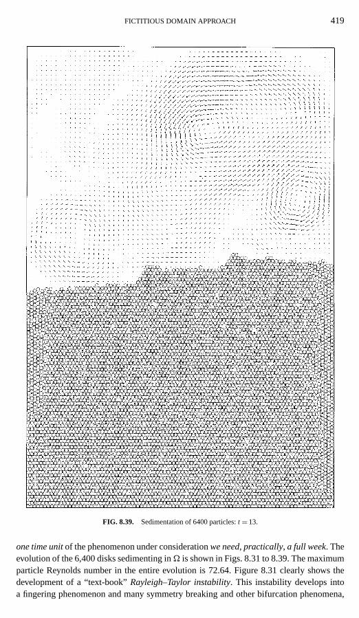
FICTITIOUS DOMAIN APPROACH 419
FIG. 8.39. Sedimentation of 6400 particles:t = 13.
one time unitof the phenomenon under considerationwe need, practically, a full week. Theevolution of the 6,400 disks sedimenting inÄ is shown in Figs. 8.31 to 8.39. The maximumparticle Reynolds number in the entire evolution is 72.64. Figure 8.31 clearly shows thedevelopment of a “text-book”Rayleigh–Taylor instability. This instability develops intoa fingering phenomenon and many symmetry breaking and other bifurcation phenomena,

420 GLOWINSKI ET AL.
including drafting, kissing, and tumbling, take place at various scales and times; similarlyvortices of various scales develop and for a while the phenomenon is clearly chaotic, whichis not surprising after all for a 6400-body problem. Finally, the particles settle at the bottomof the cavity and the fluid returns to rest.
Actually, the authors of the present article are currently preparing another one where itwill be shown that the analytical theory of Rayleigh–Taylor instabilities, when applied tothe situation prevailing here att = 0, predicts a behavior of the mixture for 0≤ t ≤ 1 veryclose, quantitatively, to that directly simulated via the computational techniques discussedin this article.
Remark 8.5. In the above calculation we have assumed that the disks have identicaldiameterd and densityρs; in fact the methods discussed in this article can handle thosesituations where diameters and densities (and even shapes) differ.
8.9. Fluidization of a Bed of 1,204 Spherical Particles
We consider here the simulation of fluidization in a bed of 1204 spherical particles. Thecomputational domain isÄ = (0, 0.6858)× (0, 20.3997)× (0, 44.577). The thickness of
FIG. 8.40. Fluidization of 1204 spherical particles: positions of the particles att = 0 and 1.5.

FICTITIOUS DOMAIN APPROACH 421
this bed is slightly larger than the diameter of the particles, which isd = 0.635, so there isonly one layer of balls in the 0x2 direction. In [49] many experimental results related to thistype of “almost two-dimensional” beds are presented. The fluid is incompressible, viscous,and Newtonian; its density isρf = 1 and its viscosity isνf = 10−2. We suppose that att = 0the fluid and the particles are at rest. The boundary condition for the velocity field is
u(t) =
0 on the four vertical walls,
5
00
1− e−50t
on the two horizontal walls.
The density of the balls isρs = 1.14. We suppose that the fluid can enter and leave thebed but that the balls have to stay in it; i.e., they cannot cross0 (=∂Ä) to leave thebed. The mesh size for the velocity field ishÄ = 0.06858 (corresponding to 2× 10⁶ ver-tices for the velocity mesh), while it ishp = 2hÄ for the pressure (corresponding to 2.9×10⁵ vertices for the pressure mesh). The time step is1t = 10−3. The parameterε used inthe collision model is 5× 10⁻⁷ and we takeρ = hÄ as the thickness of the safety zone
FIG. 8.41. Fluidization of 1204 spherical particles: positions of the particles att = 3 and 4.5.

422 GLOWINSKI ET AL.
FIG. 8.42. Fluidization of 1204 spherical particles: positions of the particles att = 6 and 7.
around each particle. The initial position of the balls is shown in Fig. 8.40. After we be-gin pushing the balls up, we observe that the inflow creates cavities propagating amongthe balls in the bed. Since the inflow velocity is much higher than the critical fluidizationvelocity (of order 2.5 here), many balls are pushed directly to the top of the bed. Thoseballs at the top of the bed are stable and closely packed while the others are circling aroundat the bottom of the bed. These numerical results are very close to experimental onesand have been visualized in Figs. 8.40 to 8.43. In the simulation, the maximum particleReynolds number is 1512 while the maximum averaged particle Reynolds number is 285.The computations were done on an SGI Origin 2000, using a partially parallelized code;the computational time is approximately 110 s/time step. The advection–diffusion has beentreated by a least-squares/conjugate gradient.
The authors of this article are currently preparing an article specifically dedicated tothe above simulations; it will contain comparisons between the results obtained by directnumerical simulation and the experimental ones measured in the laboratory of the fourthauthor at the University of Minnesota.

FICTITIOUS DOMAIN APPROACH 423
FIG. 8.43. Fluidization of 1204 spherical particles: positions of the particles att = 8 and 10.
9. CONCLUSION
We have presented in this article a distributed Lagrange-multiplier-based fictitious domainmethodology for the simulation of flow with moving boundaries. This novel methodologyallows thedirect numerical simulationof fairly complicated phenomena such as particulateflow, including sedimentation and fluidization. Other goals include:
• 3-D particulate flow with large numbers of particles of different sizes, shapes, anddensities;• particulate flow for viscoelastic liquids, such as Oldroyd-B.
ACKNOWLEDGMENTS
We acknowledge the helpful comments and suggestions of E. J. Dean, V. Girault, J. He, Y. Kuznetsov, Yong-Jun Lin, G. Rodin, A. Sameh, V. Sarin, and P. Singh, and also the support of the Supercomputing Institute at theUniversity of Minnesota concerning the use of an SGI Origin 2000. We acknowledge also the support of the NSF(Grants ECS-9527123, CTS-9873236, and DMS-9973318) and Dassault Aviation. The assistance of P. Muscarellois also acknowledged.

424 GLOWINSKI ET AL.
REFERENCES
1. H. H. Hu, N. A. Patankar, and M. Y. Zhu, Direct numerical simulations of fluid–solid systems using Arbitrary-Lagrangian-Eulerian technique,J. Comput. Phys., this issue.
2. R. Glowinski, T. I. Hesla, D. D. Joseph, T. W. Pan, and J. Periaux, Distributed Lagrange multiplier methodsfor particulate flows, inComputational Science for the 21st Century, edited by M. O. Bristeau, G. J. Etgen,W. Fitzgibbon, J. L. Lions, J. P´eriaux, and M. F. Wheeler (Wiley, Chichester, 1997), pp. 270–279.
3. R. Glowinski, T. W. Pan, T. I. Hesla, D. D. Joseph, and J. Periaux, A fictitious domain method with distributedLagrange multipliers for the numerical simulation of particulate flow, inDomain Decomposition Methods 10,edited by J. Mandel, C. Farhat, and X. C. Cai (AMS, Providence, RI, 1998), pp. 121–137.
4. T. W. Pan, R. Glowinski, T. I. Hesla, D. D. Joseph, and J. Periaux, Numerical simulation of the Rayleigh–Taylor instability for particulate flow, inProceedings of the Tenth International Conference on Finite El-ements in Fluids, January 5–8, 1998, Tucson, Arizona, edited by M. Hafez and J. C. Heinrich, pp. 217–222.
5. R. Glowinski, T. W. Pan, T. I. Hesla, and D. D. Joseph, A distributed Lagrange multiplier/fictitious domainmethod for particulate flow,Int. J. Multiphase Flow25(5), 755–794 (1999).
6. R. Glowinski, T. W. Pan, T. I. Hesla, D. D. Joseph, and J. Periaux, A distributed Lagrange multiplier/fictitiousdomain method for flows around moving rigid bodies: Application to particulate flow,Int. J. Numer. Meth.Fluids30, 1043–1066 (1999).
7. R. Glowinski, T. W. Pan, T. I. Hesla, D. D. Joseph, and J. Periaux, A distributed Lagrange multiplier/fictitiousdomain method for the simulation of flows around moving rigid bodies: Application to particulate flow,Comp.Meth. Appl. Mech. Eng.184, 241–267 (2000).
8. R. Glowinski, T. W. Pan, and D. D. Joseph, Fictitious domain methods for particulate flow in two and threedimensions, inProceedings of the International Conference on the Mathematics of Finite Elements and theirApplications (MAFELAP 99), edited by J. R. Whiteman, in press.
9. B. Desjardins and M. J. Esteban, On weak solution for fluid–rigid structure interaction: Compressible andincompressible models,Arch. Rational Mech. Anal.146, 59–71 (1999).
10. H. H. Hu, Direct simulation of flows of solid–liquid mixtures,Int. J. Multiphase Flow22, 335–352 (1996).
11. A. Johnson and T. Tezduyar, 3-D simulation of fluid–particle interactions with the number of particles reaching100,Comp. Meth. Appl. Mech. Eng.145, 301–321 (1997).
12. B. Maury and R. Glowinski, Fluid–particle flow: A symmetric formulation,C. R. Acad. Sci. Paris324(1),1079–1084 (1997).
13. C. S. Peskin, Numerical analysis of blood flow in the heart,J. Comput. Phys.25, 220–252 (1977).
14. C. S. Peskin and D. M. McQueen, Modeling prosthetic heart valves for numerical analysis of blood flow inthe heart,J. Comput. Phys.37, 113–132 (1980).
15. C. S. Peskin, Lectures on mathematical aspects of physiology,Lect. Appl. Math.19, 69–107 (1981).
16. A. L. Fogelson and C. S. Peskin, A fast numerical method for solving the three-dimensional Stokes equationsin the presence of suspended particles,J. Comput. Phys.79, 50–69 (1988).
17. K. Hofler, M. Muller, S. Schwarzer, and B. Wachman, Interacting particle–liquid systems, inHigh PerformanceComputing in Science and Engineering, edited by E. Krause and W. Jager (Springer-Verlag, Berlin, 1998),pp. 54–64.
18. N. A. Patankar, P. Singh, D. D. Joseph, R. Glowinski, and T. W. Pan, A new formulation of the distributedLagrange multiplier/fictitious domain method for particulate flows,Int. J. Multiphase Flow26, 1509–1524(2000).
19. Y. Achdou and Y. Kuznetsov, Algorithms for the mortar element method, inDomain Decomposition Methodsin Sciences and Engineering, edited by R. Glowinski, J. Periaux, Z.-C. Shi, and O. Widlund (Wiley, Chichester,1997), pp. 33–42.
20. C. L. Brooks, M. Karplus, and B. M. Pettitt, Proteins:A Theoretical Perspective of Dynamics, Structure, andThermodynamics(Wiley, New York, 1988).
21. N. Kikuchi and J. T. Oden,Contact Problems in Elasticity: A Study of Variational Inequalities and FiniteElement Methods(SIAM, Philadelphia, 1988).

FICTITIOUS DOMAIN APPROACH 425
22. F. Bertrand, P. A. Tanguy, and F. Thibault, A three-dimensional fictitious domain method for incompressiblefluid flow problem,Int. J. Numer. Meth. Fluids25, 719–736 (1997).
23. F. Brezzi and M. Fortin,Mixed and Hybrid Finite Element Methods(Springer-Verlag, New York, 1991).
24. J. E. Roberts and J. M. Thomas, Mixed and hybrid methods, inHandbook of Numerical Analysis, Vol. II,edited by P. G. Ciarlet and J. L. Lions (North-Holland, Amsterdam, 1991) pp. 523–639.
25. V. Girault, R. Glowinski, and T. W. Pan, A fictitious-domain method with Lagrange multipliers for the Stokesproblem, inApplied Nonlinear Analysis, edited by A. Sequeira, H. B. de Veiga, and J. H. Videman (KluwerAcademic/Plenum, New York, 1999), pp. 159–174.
26. A. J. Chorin, A numerical method for solving incompressible viscous flow problems,J. Comput. Phys.2,12–26 (1967).
27. A. J. Chorin, On the convergence of discrete approximation to the Navier–Stokes equations,Math. Comp.23,341–353 (1968).
28. A. J. Chorin, Numerical study of slightly viscous flow,J. Fluid Mech.57, 785–796 (1973).
29. R. Glowinski and O. Pironneau, Finite element methods for Navier–Stokes equations,Annu. Rev. FluidMechan.24, 167–204 (1992).
30. S. Turek,Efficient Solvers for Incompressible Flow Problems: An Algorithmic and Computational Approach(Springer-Verlag, Berlin, 1999).
31. G. I. Marchuk, Splitting and alternating direction methods, inHandbook of Numerical Analysis, Vol. I, editedby P. G. Ciarlet and J. L. Lions (North-Holland, Amsterdam, 1990), pp. 197–462.
32. J. T. Beale and A. Majda, Rates of convergence for viscous splitting of the Navier–Stokes equations,Math.Comp.37, 243–260 (1981).
33. E. J. Dean and R. Glowinski, A wave equation approach to the numerical solution of the Navier–Stokesequations for incompressible viscous flow,C. R. Acad. Sci. Paris325(1), 789–791 (1997).
34. E. J. Dean, R. Glowinski, and T. W. Pan, A wave equation approach to the numerical simulation of incom-pressible viscous fluid flow modeled by the Navier–Stokes equations, inMathematical and Numerical Aspectsof Wave Propagation, edited by J. A. De Santo (SIAM, Philadelphia, 1998), pp. 65–74.
35. M. Fortin and R. Glowinski,Augmented Lagrangian Methods(North-Holland, Amsterdam, 1983).
36. R. Glowinski and P. Le Tallec,Augmented Lagrangians and Operator Splitting Methods in Nonlinear Me-chanics(SIAM, Philadelphia, 1989).
37. R. Glowinski,Numerical Methods for Nonlinear Variational Problems(Springer-Verlag, New York, 1984).
38. O. Pironneau,Finite Element Methods for Fluids(Wiley, Chichester, 1989).
39. P. Parthasarathy,Application of a Wave-like Equation Method for Newtonian and Non-Newtonian Flows,Master thesis (Department of Mechanical Engineering, University of Houston, Houston, Texas, 1999).
40. J. Martikainen, T. Rossi, and J. Toivanen, Application of algebraic fictitious domain methods for solving thegeneralized Stokes problem, inBook of Abstracts of the Third European Conference on Numerical Mathematicsand Advanced Applications (ENUMATH99), Jyvaskyla, Finland, July 26–30, 1999, p. 168.
41. L. Schwartz,Theorie des Distributions(Herman, Paris, 1966).
42. R. Clift, J. R. Grace, and M. E. Weber,Bubbles, Drops, and Particles, Academic Press, New York, 1978.
43. R. Glowinski, Finite element methods for the numerical simulation of incompressible viscous flow. Introduc-tion to the control of the Navier–Stokes equations, inVortex Dynamics and Vortex Methods, edited by C. R.Anderson and C. Greengard (Am. Math. Soc., Providence, RI, 1991), pp. 219–301.
44. T. W. Pan, Numerical simulation of the motion of a ball falling in an incompressible viscous fluid,C. R. Acad.Sci. Paris327(2,b), 1035–1038 (1999).
45. G. H. Golub and C. Van Loan,Matrix Computations(Johns Hopkins Univ. Press, Baltimore, 1996).
46. T. W. Pan, V. Sarin, R. Glowinski, A. Sameh, and J. Periaux, A fictitious domain method with Lagrangemultipliers for the numerical solution of particular flow and its parallel implementation, inParallel Computa-tional Fluid Dynamics: Development and Applications of Parallel Technology, edited by C. A. Lin, A. Ecer,N. Satofuka, P. Fox, and J. Periaux (North-Holland, Amsterdam, 1999), pp. 467–474.
47. J. B. Ritz and J. P. Caltagirone, A numerical continuous model for the hydrodynamics of fluid particle systems,Int. J. Numer. Meth. Fluids30, 1067–1090 (1999).

426 GLOWINSKI ET AL.
48. J. Feng, H. H. Hu, and D. D. Joseph, Direct simulation of initial value problems for the motion of solid bodiesin a Newtonian fluid. 1. Sedimentation,J. Fluid Mech.261, 95–134 (1994).
49. A. F. Fortes, D. D. Joseph, and T. S. Lundgren, Nonlinear mechanics of fluidization of beds of sphericalparticles,J. Fluid Mech.177, 467–483 (1987).
50. R. R. Huilgol and N. Phan-Thien,Fluid Mechanics of Viscoelasticity(Elsevier, Amsterdam, 1997).
51. D. D. Joseph,Fluid Dynamics of Viscoelastic Liquids(Springer-Verlag, New York, 1990).
52. D. D. Joseph and Y. J. Liu, Orientation of long bodies falling in a viscoelastic liquid,J. Rheology37, 961–983(1993).
53. H. H. Hu, D. D. Joseph, and A. F. Fortes, Experiments and direct simulation of fluid particle motions,Int.Vid. J. Eng. Res.2, 17 (1997).
54. D. P. Young, R. G. Melvin, M. B. Bieterman, F. T. Johnson, S. S. Samanth, and J. E. Bussoletti, A locallyrefined finite rectangular grid finite element method. Application to computational physics,J. Comput. Phys.92, 1–66 (1991).
55. M. C. Roco,Particulate Two-Phase Flow(Butterworth-Heinemann, Boston, 1993).