A Dynamic Level-k Model in Games

Teck-Hua Ho and Xuanming Su∗

September 1, 2010

Backward induction is perhaps the most widely accepted principle for predicting

behavior in extensive-form games. In experiments, however, players frequently

violate this principle. An alternative is a 2-parameter “dynamic level-k” model,

where players choose a rule from a rule hierarchy. The rule hierarchy is itera-

tively defined such that the level-k rule is a best-response to the level-(k− 1) rule

and the level-∞ rule corresponds to backward induction. Players choose rules

based on their best guesses of others’ rules and use past plays to improve their

guesses. The model captures two systematic violations of backward induction,

namely limited induction and time unraveling and helps to resolve paradoxical

behaviors in the centipede game, repeated prisoner’s dilemma, and chain store

game, three canonical games used to demonstrate the failure of backward induc-

tion. The dynamic level-k model can also be considered as a tracing procedure

for backward induction because the former always converges to the latter in the

limit.

∗Haas School of Business, University of California at Berkeley. Authors are listed in alphabetical order.

We thank Colin Camerer and Juin-Kuan Chong for collaboration in the project’s early stages, and Vince

Crawford for extremely helpful comments. We are also grateful for constructive feedback from seminar partic-

ipants at University of California at Berkeley, University of Pennsylvania, and the Oxford University. Direct

correspondence to any of the authors. Ho and Su: Haas School of Business, University of California at Berke-

ley, Berkeley, CA 94720-1900, Email: Ho: hoteck@haas.berkeley.edu; Su: xuanming@haas.berkeley.edu.

1

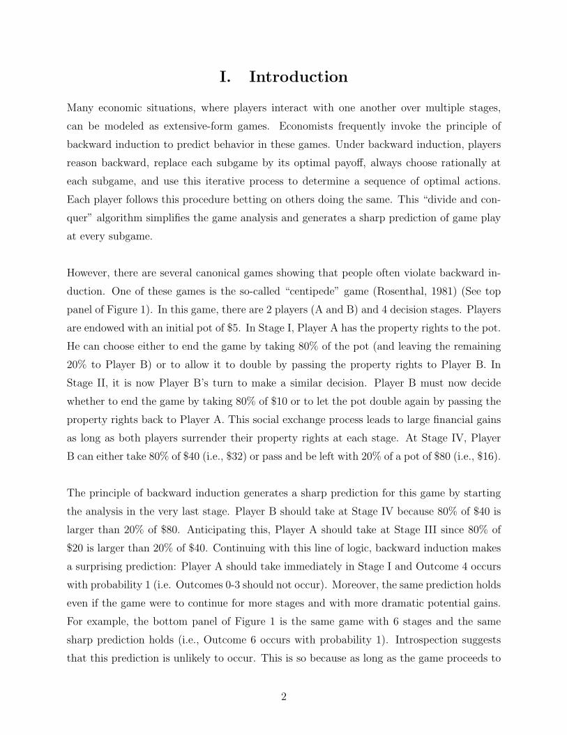
I. Introduction

Many economic situations, where players interact with one another over multiple stages,

can be modeled as extensive-form games. Economists frequently invoke the principle of

backward induction to predict behavior in these games. Under backward induction, players

reason backward, replace each subgame by its optimal payoff, always choose rationally at

each subgame, and use this iterative process to determine a sequence of optimal actions.

Each player follows this procedure betting on others doing the same. This “divide and con-

quer” algorithm simplifies the game analysis and generates a sharp prediction of game play

at every subgame.

However, there are several canonical games showing that people often violate backward in-

duction. One of these games is the so-called “centipede” game (Rosenthal, 1981) (See top

panel of Figure 1). In this game, there are 2 players (A and B) and 4 decision stages. Players

are endowed with an initial pot of $5. In Stage I, Player A has the property rights to the pot.

He can choose either to end the game by taking 80% of the pot (and leaving the remaining

20% to Player B) or to allow it to double by passing the property rights to Player B. In

Stage II, it is now Player B’s turn to make a similar decision. Player B must now decide

whether to end the game by taking 80% of $10 or to let the pot double again by passing the

property rights back to Player A. This social exchange process leads to large financial gains

as long as both players surrender their property rights at each stage. At Stage IV, Player

B can either take 80% of $40 (i.e., $32) or pass and be left with 20% of a pot of $80 (i.e., $16).

The principle of backward induction generates a sharp prediction for this game by starting

the analysis in the very last stage. Player B should take at Stage IV because 80% of $40 is

larger than 20% of $80. Anticipating this, Player A should take at Stage III since 80% of

$20 is larger than 20% of $40. Continuing with this line of logic, backward induction makes

a surprising prediction: Player A should take immediately in Stage I and Outcome 4 occurs

with probability 1 (i.e. Outcomes 0-3 should not occur). Moreover, the same prediction holds

even if the game were to continue for more stages and with more dramatic potential gains.

For example, the bottom panel of Figure 1 is the same game with 6 stages and the same

sharp prediction holds (i.e., Outcome 6 occurs with probability 1). Introspection suggests

that this prediction is unlikely to occur. This is so because as long as the game proceeds to

2

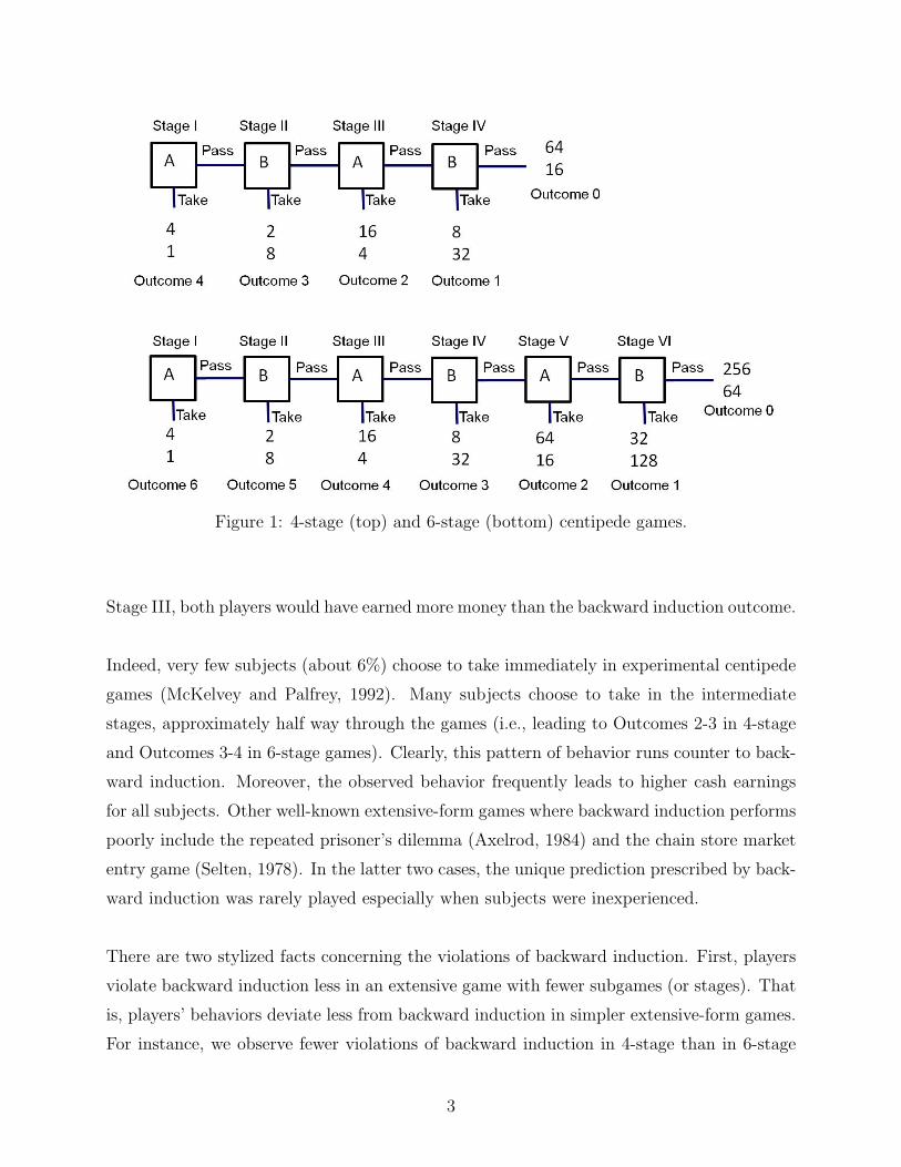
Figure 1: 4-stage (top) and 6-stage (bottom) centipede games.

Stage III, both players would have earned more money than the backward induction outcome.

Indeed, very few subjects (about 6%) choose to take immediately in experimental centipede

games (McKelvey and Palfrey, 1992). Many subjects choose to take in the intermediate

stages, approximately half way through the games (i.e., leading to Outcomes 2-3 in 4-stage

and Outcomes 3-4 in 6-stage games). Clearly, this pattern of behavior runs counter to back-

ward induction. Moreover, the observed behavior frequently leads to higher cash earnings

for all subjects. Other well-known extensive-form games where backward induction performs

poorly include the repeated prisoner’s dilemma (Axelrod, 1984) and the chain store market

entry game (Selten, 1978). In the latter two cases, the unique prediction prescribed by back-

ward induction was rarely played especially when subjects were inexperienced.

There are two stylized facts concerning the violations of backward induction. First, players

violate backward induction less in an extensive game with fewer subgames (or stages). That

is, players’ behaviors deviate less from backward induction in simpler extensive-form games.

For instance, we observe fewer violations of backward induction in 4-stage than in 6-stage

3

game (see Figure 1). We call this behavioral tendency limited induction. Second, players

unravel over time as they play the same extensive-form game repeatedly. That is, players’

behaviors converge towards backward induction over time. For instance, we observe fewer

violations of backward induction in Round 10 than in Round 1 of the experimental centipede

games in Figure 1. This behavioral tendency is termed time unraveling. The inability of

backward induction to account for the two empirical stylized facts poses modeling challenges

for economists.

In this paper, we propose an alternative to backward induction, a “dynamic level-k” model,

that generalizes backward induction and accounts for limited induction and time unraveling.

In the dynamic level-k model, players choose a level-k rule, Lk (k = 0, 1, 2, 3 . . .), from a set

of iteratively defined rules and the chosen rule prescribes an action at each subgame (Stahl

and Wilson, 1995; Stahl, 1996; Ho et al. 1998; Costa-Gomes et al. 2001; Costa-Gomes and

Crawford, 2006; Crawford and Iriberri, 2007a, 2007b). Players choose a rule based on their

beliefs of others’ rules and update their beliefs based on game history (cf. Stahl, 2000). The

rule hierarchy is defined such that the level-k rule best-responds to the level-(k− 1) and the

level-∞ corresponds to backward induction.

Players are heterogenous in that they have different initial guesses of others’ rules and con-

sequently choose different initial rules. The distribution of the initial guesses are assumed to

follow a Poisson distribution. These initial guesses are updated based on game history and

lead to players choosing different rules over time.

We prove that the dynamic level-k model can account for limited induction and time unravel-

ing properties in the centipede game, the finitely repeated prisoner’s dilemma, and the chain

store game. Consequently our model can explain passing in the centipede game, cooperation

in the repeated prisoner’s dilemma, and fighting by the incumbent in the chain-store game.

All these behaviors are considered paradoxical under backward induction but are predicted

by the dynamic level-k model. In addition, the dynamic level-k model is able to capture the

empirical stylized fact that behaviors will eventually converge to backward induction over

time, and hence the former can be considered as a tracing procedure for the latter.

We fit our model using experimental data on the centipede game from McKelvey and Palfrey

4

(1992) and find that our model fits the data significantly better than backward induction

and static level-k model. We rule out two alternative explanations including the reputation-

based model of Kreps et al. (1982) and a model allowing for social preferences (Fehr and

Schmidt, 1999). Overall, it appears that the dynamic level-k model can be an empirical

alternative to backward induction.

The rest of the paper is organized as follows. Section II discusses the backward induction

principle and its violations. Section III formulates the dynamic level-k model and applies it

to explain paradoxical behaviors in centipede game, iterated prisoner’s dilemma, and chain

store game. Section IV fits the dynamic level-k model to data from experimental centipede

game and rules out two alternative explanations. Section V concludes.

II. Violations of Backward Induction

Backward induction uses an iterative process to determine an optimal action at each sub-

game. The predictive success of this iterative reasoning process hinges on players’ complete

confidence in others applying the same logic in arriving at the backward induction outcomes.

If players have doubts about others applying backward induction, it is in their best interest

to deviate from backward induction’s prescription. Indeed, subjects do and profitably so in

many experiments.

If a player i chooses a behavioral rule Li that is different from backward induction (L∞), one

would like to develop a formal measure to quantify this deviation. Consider an extensive-

form game G with S subgames. We can define the deviation for a set of behavioral rules

Li(i = 1, . . . I), one for each player, in game G as:

δ(L1, . . . , LI , G) =1

S

S∑s=1

[1

Ns

Ns∑i=1

Ds(Li, L∞)

], (II.1)

where Ds(Li, L∞) is 1 if player i chooses an action at subgame s that is different from the

prescription of backward induction and 0 otherwise, and Ns is the number of players who

are active at subgame s. Note that the measure varies from 0 to 1, where 0 indicates that

players’ actions perfectly match the predictions of backward induction and 1 indicates that

5

none of the players’ actions agree with the predictions of backward induction.

Let’s illustrate the deviation measure using a 4-stage centipede game. Let the behavioral

rules adopted by player A and B be LA = {P,−, T,−} and LB = {−, P,−, T} respectively

(that is, player A will pass in Stage I and take in Stage III, and player B will pass in Stage

II and take in Stage IV). Then the game will end in Stage III (i.e., Outcome 2). The de-

viation will be δ(LA, LB, G) = 14[1 + 1 + 0 + 0] = 1

2. Similarly, if LA = {P,−, T,−} and

LB = {−, T,−, T}, then the game will end in Stage Stage II (i.e., Outcome 3). This gives

δ(LA, LB, G) = 14[1 + 0 + 0 + 0] = 1

4, which is smaller. Note that the latter behavioral rules

are closer to backward induction than the former behavioral rules.

Using the above deviation measure, we can formally state the two systematic violations of

backward induction as follows:

1. Limited Induction: Consider two extensive-form games G and G′ where G′ is a proper

subgame of G. The deviation from backward induction is equal or larger in G than

in G′. That is, the deviation from backward induction increases in S. Formally, for a

group of players who adopt the same set of behavioral rules (Li, i = 1, . . . , I) in games

G and G′, we have δ(L1, . . . , LI , G) ≥ δ(L1, . . . , LI , G′). Consequently, a good behav-

ioral model must predict a larger deviation in G than in G′ to be behaviorally plausible.

2. Time Unraveling: If an extensive-form game G is played repeatedly over time, the de-

viation from backward induction at time t converges to zero as t→∞. That is, time

unraveling implies δ(L1(t), . . . , LI(t), G) → 0 as t → ∞. Therefore, game outcomes

will be consistent with backward induction after sufficiently many repetitions.

Let’s illustrate limited induction and time unraveling using data from McKelvey and Palfrey

(1992). These authors conducted an experiment to study behavior in 4-stage and 6-stage

centipede games. Each subject was assigned to one of these games and played the same

game in the same role 10 times. For each observed outcome in a game play, we can compute

6

the deviation from backward induction using Equation (II.1).1

Figure 2: Deviations from backward induction in the first round of the 4-stage and 6-stage

centipede games (Data from McKelvey and Palfrey, 1992).

Figure 2 plots the cumulative distributions of deviations from backward induction in the

first round of the 4-stage and 6-stage games respectively. The thick line corresponds to the

4-stage game and the thin line corresponds to the 6-stage game. The curve for the 6-stage

game generally lies to the right of the curve for the 4-stage game except for high deviation

values.2 The plot is suggestive that the limited induction property holds in this data set.

Figure 3 plots the cumulative distributions of deviations from backward induction in the

first and the final round of the 4-stage game. The thick line corresponds to the first round

and the thin line corresponds to the final round of game plays (similar results occur for the

6-stage game). As shown, the curve for the first round lies to the right of the curve for the

1Since subjects did not indicate what they would have chosen in every stage (i.e., data were not collected

using the strategy method), we did not observe what the subjects would have done in subsequent stages if

the game ended in an earlier stage. In computing the deviation, we assume that subjects always choose to

take in stages beyond where the game ends. Therefore, the derived measure is a conservative estimate of the

deviation from backward induction.2The empirical proportions are (0,0.28,0.38,0.24,0.10) for Outcomes 4,3,2,1,0 in the 4-stage game and

(0,0.10,0.10,0.31,0.35,0.10,0.03) for Outcomes 6,5,4,3,2,1,0 in the 6-stage game.

7

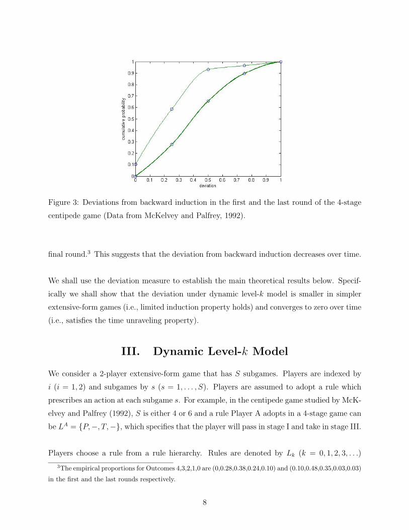
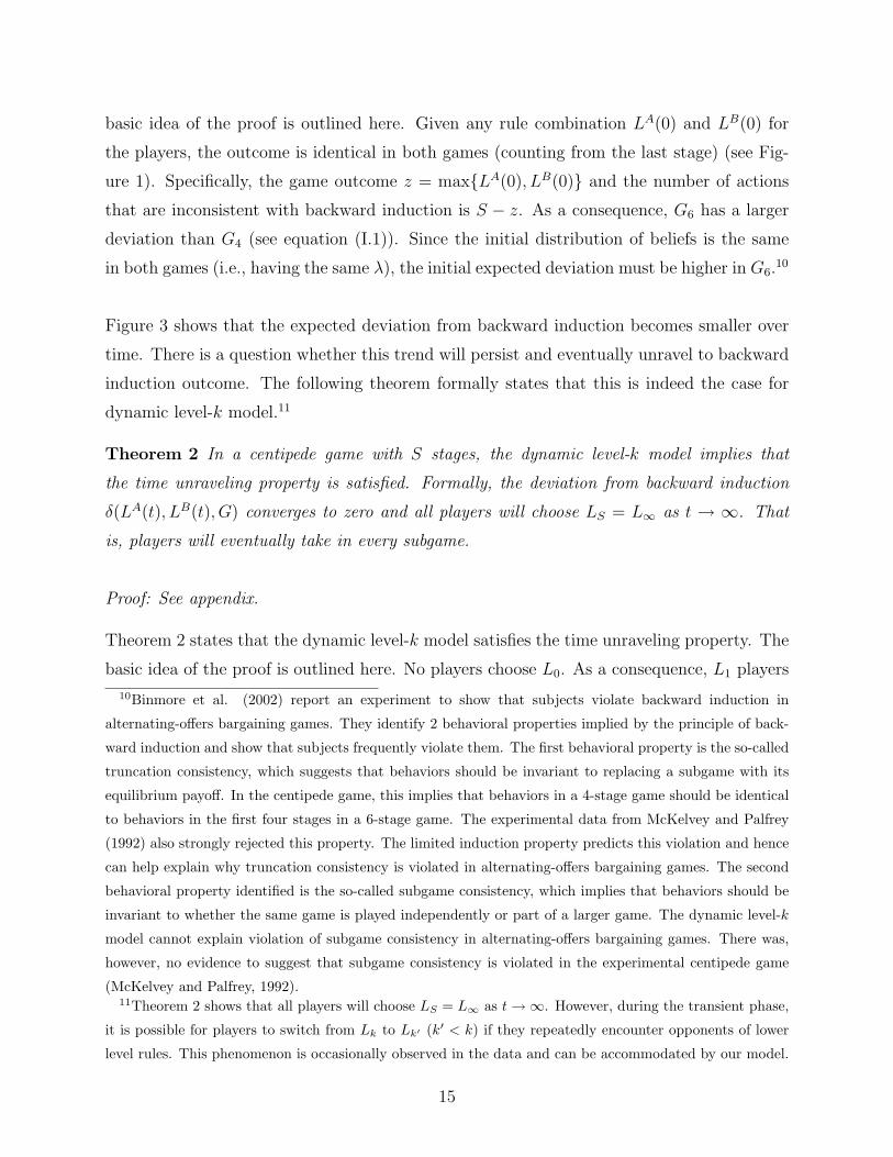
Figure 3: Deviations from backward induction in the first and the last round of the 4-stage

centipede game (Data from McKelvey and Palfrey, 1992).

final round.3 This suggests that the deviation from backward induction decreases over time.

We shall use the deviation measure to establish the main theoretical results below. Specif-

ically we shall show that the deviation under dynamic level-k model is smaller in simpler

extensive-form games (i.e., limited induction property holds) and converges to zero over time

(i.e., satisfies the time unraveling property).

III. Dynamic Level-k Model

We consider a 2-player extensive-form game that has S subgames. Players are indexed by

i (i = 1, 2) and subgames by s (s = 1, . . . , S). Players are assumed to adopt a rule which

prescribes an action at each subgame s. For example, in the centipede game studied by McK-

elvey and Palfrey (1992), S is either 4 or 6 and a rule Player A adopts in a 4-stage game can

be LA = {P,−, T,−}, which specifies that the player will pass in stage I and take in stage III.

Players choose a rule from a rule hierarchy. Rules are denoted by Lk (k = 0, 1, 2, 3, . . .)

3The empirical proportions for Outcomes 4,3,2,1,0 are (0,0.28,0.38,0.24,0.10) and (0.10,0.48,0.35,0.03,0.03)

in the first and the last rounds respectively.

8

and are generated from iterative best-responses. In general, Lk is a best-response to Lk−1

at every subgame, and L∞ corresponds to backward induction. Under this rule hierarchy,

the deviation from backward induction (see equation (I.1)) is smaller if player i adopts a

higher level rule (while others keep their rule at the same level). In fact, ceteris paribus, the

deviation from backward induction is monotonically decreasing in k. In other words, the

level of a player’s rule captures its closeness to backward induction.

Note that Lk prescribes the same behavior as backward induction in any extensive-form

game with k or fewer subgames. In this regard, Lk can be viewed as a limited backward

induction rule that only works for simpler games. Putting it this way, a higher level rule is

more likely to coincide with backward induction in a wider class of games so that the level

of a rule measures its degree of resemblance to backward induction.

If every player is certain about others’ rationality, all players will choose L∞. However, if

players have doubts about others’ rationality, it is not in their best interest to apply back-

ward induction. Instead, they should form beliefs over rules adopted by others4 and choose a

best-response rule in order to maximize their expected payoffs. Therefore, under the model,

players are subjective expected utility maximizers. In this regard, the dynamic level-k model

is similar to the notion of rationalizable strategic behavior (Bernheim, 1984; Pearce, 1984;

Reny, 1992) except that players always choose a rule from the defined rule hierarchy.

In a typical laboratory experiment, players frequently play the same extensive-form game

repeatedly. After each game round, players observe the rules used by their opponents and

update their beliefs by tracking the frequencies of rules played by opponents in the past. Let

player i’s rule counts at the end of round t be N i(t) = (N i0(t), . . . , N

iS(t)) where N i

k(t) is the

cumulative count of rule Lk that has been used by opponents at the end of round t (Camerer

and Ho, 1999; Ho et al., 2007). Note that for an extensive-form game with S subgames, all

rules of level S or higher will prescribe the same action at each subgame and hence we pool

them together and collectively call them LS. Given these rule counts, player i forms a belief

4Subjects’ beliefs may depend on their knowledge of their opponents’ rationality. Players who play against

opponents who are known to be sophisticated will adopt a higher level rule. For example, Palacios-Huerta

and Volijc (forthcoming) show that many chess players playing against other equally sophisticated chess

players take immediately in the centipede game.

9

Bi(t) = (Bi0(t), . . . , B

iS(t)) where

Bik(t) =

N ik(t)∑S

k′=0Nik′(t)

. (III.1)

Bik(t) is player i’s belief of the probability that her opponent will play Lk in round t + 1.

The updating equation of the cumulative count at the end of round t is given by:

N ik(t) = N i

k(t− 1) + I(k, t) · 1, ∀k (III.2)

where I(k, t) = 1 if player i’s opponent adopts rule Lk in round t and 0 otherwise. Therefore,

players update their beliefs based on the history of game plays. This updating process is

consistent with Bayesian updating involving a multinomial distribution with a Dirichlet prior

(Fudenberg and Levine, 1998, Camerer and Ho, 1999). As a consequence of the updating

process, players may adopt a different best-response rule in round t+ 1.5

5The above updating rule assumes that subjects observe rules chosen by opponents. This is possible if

the strategy method is used to elicit subjects’ contingent action at each subgame. When the opponents’

chosen rules are not observed, the updating process is still a good approximation because subjects may have

a good guess of their opponents’ chosen rules in most simple games (e.g., centipede games). More generally,

the updating of N ik(t) depends on whether player i adopts a higher or lower level rule than her opponent.

If the opponent uses a higher level rule (e.g., the opponent takes before the player in the centipede game),

then we have like the above:

N ik(t) = N i

k(t− 1) + I(k, t) · 1 (III.3)

where I(k, t) = 1 if opponent adopts an action that is consistent with Lk in round t and 0 otherwise. If

player i adopts a higher level rule k∗ (e.g., takes before the opponent in the centipede game), the player can

only infer that the opponent has chosen some rule that is below k∗. Then we have:

N ik(t) = N i

k(t− 1) + I(k ≤ k∗) · N ik(t− 1)∑k∗

k′=0Nik′(t− 1)

(III.4)

where I(k ≤ k∗) = 1 if k ≤ k∗ and 0 otherwise. This updating process assigns a belief weight to all

lower level rules that are consistent with the observed outcome. The weight assigned to each consistent

rule is proportional to its prior belief weight. For this alternative updating process, the main results for the

centipede game (i.e., Theorems 1 and 2) still go through. However, we are not able to prove the same results

for the repeated prisoner’s dilemma and the chain store game.

10

Player i chooses the optimal rule Lk∗ in round t+ 1 from the rule hierarchy {L0, L1, . . . , LS}based on belief Bi(t) in order to maximize expected payoffs. Let aks be the specified action

of rule Lk at subgame s. Player i believes that action ak′s will be chosen with probability

Bik′(t) by the opponent. Hence, the optimal rule chosen by player i is:

k∗ = argmaxk=1,...,S

S∑s=1

{S∑

k′=1

Bik′(t) · πi(aks, ak′s)

}, (III.5)

where πi(aks, ak′s) is player i’s payoff at subgame s if i chooses rule Lk and the opponent

chooses Lk′ rule (cf. Camerer et al., 2004).

Note that we model learning across game rounds but not across stages within a game round.

This is clearly an approximation. For a general extensive-form game, a player could po-

tentially update her belief about the opponent’ rule within a round as the game unfolds.

Specifically, a player may rule out a potential rule used by her opponent if an observed

choice by the opponent at a particular stage is inconsistent with that rule. For example, in

the 4-stage centipede game, if player B observes player A passing in stage I, player B will

infer that player A’s chosen rule must be level 3 or lower. Nevertheless, we believe that the

assumption is a good starting point for 2 reasons. First, in the 3 games we study below

(centipede game, repeated prisoner’s dilemma, and chain-store game), the posterior belief at

the end of a game round remains the same whether or not within-round learning is modeled

explicitly. This is so because no new information is revealed once a player’s opponent chooses

an action that is contrary to the prior belief. For instance, in the centipede game, when a

player is surprised by an opponent who takes earlier than expected, the game ends immedi-

ately and no additional information is revealed.6 Second, within-round learning frequently

generates prediction that is contrary to observed behavior. For example, in the centipede

game, the second player who expects the first player to take immediately will be surprised

if the latter passes. If we incorporate within-round learning, this will lead the second player

to put more weights on the lower level rules. As a consequence, the second player will be

more likely to pass, which generally runs counter to the observed data.

6Similarly, in the repeated Prisoner’s dilemma, players’ subsequent actions after a defection by some

player does not contain new information as long as players choose from the rule hierarchy specified below.

In the chain store game, once the incumbent shares the market, subsequent actions by entrants will provide

no new information as long as they choose from the defined rule hierarchy.

11

We need to determine player i’s initial belief Bi(0). We define N i(0) such that N ik(0) = β

for some k and 0 otherwise where the parameter β captures the weight assigned to initial

belief. In other words, player i places all the initial weight on a particular rule k and zero

weight on all other rules. Different players have different guesses about others’ rationality

and hence place the initial weight on a different k. A player who places the initial weight on

k will choose an initial rule of Lk+1 in round 1. The heterogeneity of players’ initial beliefs

is captured by a Poisson distribution. The proportion of players who hold initial belief k is

given by:

φ(k) =e−λ · λk

k!; k = 0, . . . , S. (III.6)

For example, a φ(0) proportion of players believe that their opponents will play L0 and thus

choose L1. Similarly, a φ(k) proportion of players believe that their opponents will play Lk

and best-respond with Lk+1. All players best-respond given their beliefs in order to maximize

their expected payoffs. Note that no players will choose L0 under our model. That is, L0

only occurs in the minds of the higher level players.7

The dynamic level-k model, similar to the cognitive hierarchy (CH) model, uses a Poisson

distribution to capture player heterogeneity. The single parameter Poisson approach allows

these models to be tractably used as a building block for theoretical analysis. However,

the parsimony of a parametric approach comes with an empirical limitation. Specifically,

the Poisson distribution often implies a non-negligible proportion of L0 players in empirical

applications of the CH model (see Camerer et al., 2004). In contrast, using a general discrete

distribution, Costa-Gomes and Crawford (2006) and Crawford and Iriberri (2007a, 2007b)

show that the estimated proportion of L0 players is frequently zero. In agreement with

the above observation, our proposed dynamic level-k model assumes that there are no L0

players. Unlike the CH model, which captures heterogeneity in players’ rules, the dynamic

level-k model captures heterogeneity in players’ beliefs of others’ rules and allows players to

best-respond to their beliefs. For example, φ(0) represents the proportion of L0 players in

7In the centipede game, this implies that the dynamic level-k does not admit occurrence of outcome 0 in

4-stage and 6-stage games, where players pass all the way. No model with only self-interested players can

account for such behavior. Our model can easily be extended by incorporating social preferences in order to

capture this kind of phenomenon.

12

the CH model, but it represents, in our model, the proportion of players who believe that

their opponents play L0 and thus choose L1. Therefore, our proposed dynamic level-k model

excludes L0 players.8 In this way, the dynamic level-k model retains the parsimony of the

Poisson distribution while improving its empirical validity.

The dynamic level-k model is different from the static level-k and cognitive hierarchy models

in 3 fundamental aspects. First, players in our model are not born with a specific thinking

type. That is, players in our model are cognitively capable of choosing any rule but always

choose the level that maximizes their expected payoff. In other words, players in our model

are not constrained by reasoning ability. Second, players in our model may be aware of

others who adopt higher level rules than themselves. In other words, a player who chooses

Lk may recognize that there are others who choose Lk+1 or higher but still prefers choose

Lk because there is a large majority of players who are Lk−1 or below. On the other hand,

the static level-k and CH models assume players always believe they are the highest level

thinkers (i.e., the opponents are always of a lower level rule). Third, unlike the static level-k

and CH models, players in the dynamic level-k model may change their rules as they collect

more information and update beliefs about others. Specifically, a player who interacts with

opponents of higher level rules may advance to a higher rule. Similarly, a players who inter-

acts with opponents of lower level rules may switch to a lower level rule in order to maximize

their expected payoffs.

In summary, the dynamic level-k model has 2 parameters, β and λ. The parameter λ captures

the degree of heterogeneity in initial belief and the parameter β captures the strength of the

initial belief, which in turn determines players’ sensitivity to game history. The 2-parameter

dynamic level-k model nests several well-known special cases. When λ = ∞, it reduces to

backward induction. If β = ∞, players have a stubborn prior and never respond to game

history. This reduces our model to a variant of the static level-k model.9 Consequently, we

can empirically test whether these special cases are good approximations of behavior using

8It is possible to generalize this setup by introducing a segment of non-strategic players (level 0). Let

π be the proportion of non-strategic players and 1 − π be the proportion of strategic players (level 1 and

higher). As described above, the Poisson model can be used to describe the distribution of strategic players.

Consequently, the dynamic level-k model is simply a special case with π = 0.9Note that under the dynamic level-k model, while players may believe others are level-0, they themselves

never play level-0 rules.

13

the standard generalized likelihood principle.

Below, we apply the dynamic level-k model to explain violations of backward induction in

three canonical games. In each case, we prove that the dynamic level-k model can account

for the limited induction and time unraveling properties of the data.

A. Centipede game

McKelvey and Palfrey (1992) assume there is a proportion of players who always pass in every

subgame. To avoid over-fitting, we assume that L0 corresponds to the same strategy. That

is, we choose L0 = {P1, P2, . . . , PS−1, PS}. A player who believes her opponent uses L0 will

maximize her payoff by adopting L1 = {P1, P2, . . . , PS−1, TS}. In general, Lk best-responds

to Lk−1 so that Lk = {P1, . . . , PS−k, TS−k+1, . . . , TS}. Therefore in a centipede game with

S subgames, LS = LS+1 = . . . = L∞. Put differently, all rules LS or higher prescribe the

same action at each subgame as L∞ (the backward induction rule). Consequently, we pool

all these higher level rules together and collectively call them LS.

Under the dynamic level-k belief model, players i (i = A,B) choose rules from the rule hierar-

chy Lk (k = 0, 1, 2, 3, . . .). Denote player i’s rule in time t as Li(t). Then δ(LA(0), LB(0), G)

is the deviation from backward induction L∞ in game G at time 0. For example, if Players

A and B both play L2, the deviation is 12

in a 4-stage and 23

in a 6-stage centipede game.

Let G4 and G6 be the 4-stage and 6-stage games respectively. Then we have the following

theorem:

Theorem 1 In the centipede game, the dynamic level-k model implies that the limited in-

duction property is satisfied. Formally, if the initial distribution of beliefs is the same in both

games (i.e., having the same λ), then the expected deviation from backward induction in G4,

δ(LA(0), LB(0), G4), is smaller than in G6, δ(LA(0), LB(0), G6).

Proof: See appendix.

Theorem 1 suggests that the dynamic level-k model gives rise to a smaller deviation from

backward induction in a game with a smaller number of subgames. This result is consis-

tent with the data presented in Figure 2. The Appendix gives the detailed proof but the

14

basic idea of the proof is outlined here. Given any rule combination LA(0) and LB(0) for

the players, the outcome is identical in both games (counting from the last stage) (see Fig-

ure 1). Specifically, the game outcome z = max{LA(0), LB(0)} and the number of actions

that are inconsistent with backward induction is S − z. As a consequence, G6 has a larger

deviation than G4 (see equation (I.1)). Since the initial distribution of beliefs is the same

in both games (i.e., having the same λ), the initial expected deviation must be higher in G6.10

Figure 3 shows that the expected deviation from backward induction becomes smaller over

time. There is a question whether this trend will persist and eventually unravel to backward

induction outcome. The following theorem formally states that this is indeed the case for

dynamic level-k model.11

Theorem 2 In a centipede game with S stages, the dynamic level-k model implies that

the time unraveling property is satisfied. Formally, the deviation from backward induction

δ(LA(t), LB(t), G) converges to zero and all players will choose LS = L∞ as t → ∞. That

is, players will eventually take in every subgame.

Proof: See appendix.

Theorem 2 states that the dynamic level-k model satisfies the time unraveling property. The

basic idea of the proof is outlined here. No players choose L0. As a consequence, L1 players

10Binmore et al. (2002) report an experiment to show that subjects violate backward induction in

alternating-offers bargaining games. They identify 2 behavioral properties implied by the principle of back-

ward induction and show that subjects frequently violate them. The first behavioral property is the so-called

truncation consistency, which suggests that behaviors should be invariant to replacing a subgame with its

equilibrium payoff. In the centipede game, this implies that behaviors in a 4-stage game should be identical

to behaviors in the first four stages in a 6-stage game. The experimental data from McKelvey and Palfrey

(1992) also strongly rejected this property. The limited induction property predicts this violation and hence

can help explain why truncation consistency is violated in alternating-offers bargaining games. The second

behavioral property identified is the so-called subgame consistency, which implies that behaviors should be

invariant to whether the same game is played independently or part of a larger game. The dynamic level-k

model cannot explain violation of subgame consistency in alternating-offers bargaining games. There was,

however, no evidence to suggest that subgame consistency is violated in the experimental centipede game

(McKelvey and Palfrey, 1992).11Theorem 2 shows that all players will choose LS = L∞ as t→∞. However, during the transient phase,

it is possible for players to switch from Lk to Lk′ (k′ < k) if they repeatedly encounter opponents of lower

level rules. This phenomenon is occasionally observed in the data and can be accommodated by our model.

15

will learn that other players are L1 or higher. Using our notation, this means that Bi0(t)

will decline over time and the speed of decline depends on the initial belief weight β. For a

specific β, there is a corresponding number of rounds after which all L1 players will move up

to L2 or higher. No players will then choose L0 and L1. In the same way, L2 players will learn

that other players are L2 or higher and will eventually move to L3 or higher. Consequently,

we will see a ‘domino’ phenomenon whereby lower level players will successively disappear

from the population. In this regard, players believe that others become more sophisticated

over time and correspondingly do so themselves. In the limit, all players converge to LS (and

learning stops).

The proof also reveals an interesting insight. The number of rounds it takes for Lk to disap-

pear is increasing in k. For example, when β = 1, it takes 6 rounds for L0 to disappear and

another 42 rounds for L1 to disappear. In general, for an initial belief weight β, it takes a

total of (7k − 1)β rounds for rule Lk to disappear. Note that each higher level rule takes an

exponentially longer time to be eliminated from the population.12 This result suggests that

time unraveling occurs rather slowly in the centipede game. In the experiments conducted by

McKelvey and Palfrey (1992), there are only 10 game rounds and no substantial learning is

observed. In Section III, we fit the dynamic level-k model and show that only L1 disappears

in their data set.

B. Finitely Repeated Prisoner’s Dilemma

In the finitely repeated prisoner’s dilemma, backward induction prescribes that all players

should defect in every repetition or subgame (see Figure 4 for a game with 10 repetitions).

This is because defection is a dominant strategy in every subgame. To explain cooperative

behavior, Kreps et al. (1982) assume there is a proportion of players who always adopts Tit-

For-Tat (TFT), which starts with cooperation and reciprocates by choosing the opponent’s

action in the previous round. To avoid over-fitting, we choose L0 to be TFT. A player who

believes her opponent uses L0 will play TFT until the very last round when it is optimal to

12In our model, the cumulative rule counts N ik(t) do not decay over time. If decay is allowed, that is,

N ik(t) = δ ·N i

k(t− 1) + I(k, t) · 1, then unraveling can occur at a much faster rate. For example, if δ = 0, it

takes only one round for each successively lower level rule to disappear.

16

defect. We denote this rule by L1 = {TFT,D}. L1 is better than TFT because defection

yields a payoff of 5 in the last round while cooperation yields a payoff of 3 (see Figure 4).

{TFT,D,D} is inferior to {TFT,D} because the former yields a payoff of 5+1=6 in the

last 2 rounds whereas the latter yields a payoff of 3+5=8. In general, Lk best-responds to

Lk−1 so that Lk = {TFT,k︷ ︸︸ ︷

D, . . . , D}.13 Therefore, in a repeated prisoner’s dilemma game

with S repetitions or subgames, LS = LS+1 = . . . = L∞. Put differently, all rules LS or

higher prescribe the same actions as backward induction. Consequently, we pool all these

higher level rules together and collectively call them LS.

Figure 4: Finitely repeated prisoner’s dilemma games (10 repetitions).

Theorem 3 In the finitely repeated prisoner’s dilemma, the dynamic level-k model implies

that the limited induction property is satisfied. Formally, if the initial distribution of beliefs is

the same in both games (i.e., having the same λ), then the expected deviation from backward

induction is smaller in a game with a smaller number of repetitions.

Proof: See appendix.

The basic idea of the proof is similar to the one in the centipede game. For any combination

of initial rules LA(0) and LB(0), let z = max{LA(0), LB(0)}. Then defection begins after

13Choosing cooperation initially followed by defection in the last k repetitions is also a best-response to

Lk−1. However, this simpler rule will perform poorly when played against a higher level rule. Since players

are fully aware of the entire rule hierarchy and may believe that others can use a higher level rule, it is in

their best interest to adopt a more robust TFT based rule.

17

S − z repetitions, and both players will choose defection in the remaining z − 1 repetitions.

As a consequence, a repeated prisoner’s dilemma with a larger number of repetitions will

have a longer string of sustained cooperation before defection begins. Thus the expected

deviation of backward induction is smaller for a game with fewer repetitions.

Theorem 4 In the finitely repeated prisoner’s dilemma with S repetitions, the dynamic

level-k model implies that the time unraveling property is satisfied. Formally, the deviation

from backward induction converges to zero and all players will choose LS = L∞ as t → ∞.

That is, players will eventually defect in every repetition.

Proof: See appendix.

Like before no players choose L0 (i.e., TFT) so all players will defect in the last stage. L1

players will learn over time that other players are L1 or higher and eventually move to L2

or higher (i.e., L1 disappears). After this transition, all players will defect in the second last

repetition. The same logic continues and eventually all players will defect in every single

repetition. Like before, the number of rounds for Lk to disappear is increasing in k. In

general, for an initial belief weight β, it takes a total of (2k − 1)β rounds for rule Lk to

disappear. Note that the rate of convergence is faster for repeated prisoner’s dilemma than

centipede game. In general, the rate of convergence depends on the payoff structure of the

game.

C. Chain Store Paradox

In the chain store game, an incumbent (e.g., Safeway) faces potential competition from nu-

merous entrants in separate locations and must interact with each one of them sequentially

(Selten, 1978). Entrants in each location can either choose to enter the market or stay out.

In Figure 5, there are 10 entrants. If an entrant chooses to stay out, the chain store receives

a payoff of $5 m and the entrant receives a payoff of $1 m. If the entrant enters the market,

the chain store must choose to either stage a price war or share the market with the entrant.

If the chain store fights, both players receive $0 m. If the chain store shares, both players

receive $2 m.

18

Figure 5: Chain store game with 10 entrants over 10 interactions).

Focusing on the very last entrant, the chain store will choose to share the market with the

entrant if it enters. Repeating this logic, backward induction predicts that each entrant will

enter at its respective location and the chain store will share the market with each one of

them. This seems implausible because introspection suggests that the chain store is likely

to fight at least in some of the markets and not all entrants will choose to enter in their

locations. Specifically, Selten (1978) wrote:

The disturbing disagreement between plausible game behavior and game theoretical

reasoning constitutes the chain store paradox.

To explain entry and sharing, Jung et al. (1994) and Camerer et al. (2002) assume that

there is a probability that the incumbent is a fighter type, who always fights upon entry. To

avoid over-fitting, we choose LI0 for the incumbent to be always fight conditional on entrance.

LE1 entrants who believe the incumbent uses LI0 will maximize their payoff by adopting the

so-called grim trigger rule (GTR). The GTR rule prescribes that an entrant contemplat-

ing entry will choose to stay out unless the chain store is observed to share the market in

the past. Given the sequential nature of the game, LI1 incumbent will best-respond to LE1

19

entrants by always fighting until the very last interaction when it is optimal to share the

market condition on entrance, i.e., {F, F, . . . , F, S}.

In general, LEk entrants best-respond to a LIk−1 incumbent and this implies that LEk =

{GTR,k−1︷ ︸︸ ︷

E, . . . , E}. Similarly, a LIk incumbent best-responds to LEk−1 entrants and this im-

plies that LIk = {F, F, F,k︷ ︸︸ ︷

S, . . . , S}. Therefore, in a chain store game with S interactions,

LES+1 = . . . = L∞ and LIS = LIS+1 = . . . = L∞. Put differently, all rules with level S or

higher prescribe the same actions as the rule of backward induction. Consequently, we pool

all these higher level rules together and collectively call them LES and LIS.

Note that we have defined two separate rule hierarchies, one for each role, because the incum-

bent and entrants have a different strategy space. Further, in this game, each interaction is a

sequential game where the incumbent chooses only after observing the action of the entrant.

Consequently, our rule hierarchies are defined in a zig-zag structure where LEk entrants best-

respond to LIk−1 incumbent and LIk incumbent always best-responds to LEk entrants. Note

that the zig-zag structure is for notational convenience and it does not change the main

results.

Theorem 5 In the chain store game, the dynamic level-k model implies that the limited

induction property is satisfied. Formally, if the initial distribution of beliefs is the same in

both games (i.e., having the same λ) and all entrants have the same initial belief (i.e. they

assign β to the same k), then the expected deviation from backward induction is smaller in

a game with a smaller number of interactions.

Proof: See appendix.

Let LI(0) and LE(0) be the initial rules for incumbent and all entrants respectively. For any

combination of rule LI(0) and LE(0), the outcome in the last z = max{LI(0), LE(0) − 1}interactions is the same regardless of the total number of interactions. As a consequence,

a chain store game with a larger number of repetitions will have a longer string of entrants

staying out and the incumbent fighting before entrants begin to enter. Thus the expected

deviation of backward induction is smaller for a game with fewer repetitions.

20

Theorem 6 In the chain store game with S interactions, the dynamic level-k model implies

that the time unraveling property is satisfied. Formally, the deviation from backward induc-

tion converges to zero and players will choose LS = L∞ as t → ∞. That is, every entrant

will eventually enter and incumbent will always share in every interaction.

Proof: See appendix.

The idea of the proof is similar to that in the previous two games. No incumbent will al-

ways fight. Given this fact, LE1 entrants will learn that the incumbent is LI1 or higher and

eventually will share in the last interaction. This implies that LE1 will disappear. After this

happens, the LI1 incumbent will learn that entrants are LE2 or higher. As a consequence, LI1

will eventually disappear. The same logic continues and eventually all entrants will enter

and the incumbent will share the market in every single interaction. This is consistent with

backward induction.

D. Properties of Level-0 Rule

The above rule hierarchies are generated from iterated best responses to a specific level-0

rule. To avoid over-fitting, we have used the level-0 rules from the existing literature. For

instance, following McKelvey and Palfrey (1992), we use a decision rule that passes in every

subgame as level-0 in the centipede game. Similarly, as in Kreps et al. (1982), the Tit-

For-Tat rule is used as level-0 in the repeated prisoner’s dilemma. Finally, in chain store

game, we define always fighting as level-0 for the incumbent (following Jung et al., 1994 and

Camerer et al. 2002).

There are 2 ways to formally determine the level-0 rule. First, we can structurally estimate

the level-0 rule using the data. One can parameterize the space of possible decision rules

and empirically determine the best-fitting level-0 rule. Second, one can develop a theory for

choosing a level-0 rule. We explore the latter approach below. Further research can provide

a more comprehensive analysis.

A good level-0 rule may satisfy the following 2 attractive properties:

21

1. Maximize group payoff: A level-0 player always chooses a decision rule that if others

do the same will lead to the largest total payoff for the group. For instance, in the

centipede game, if every player chooses a decision rule that passes in every stage, the

group will achieve the largest possible payoff.

2. Protect individual payoff: While maximizing group payoff, a level-0 player also ensures

that the chosen decision rule is robust against continued exploitation by others. For

instance, in the repeated prisoner’s dilemma, a level-0 who attempts to maximize group

payoff by always cooperating may be exploited by an individual who always chooses

to defect. A robust rule like Tit-For-Tat will prevent this kind of exploitation and

promote cooperative behavior.

The above two properties do not define a unique level-0 rule in all games. However, they

do narrow down the possible candidates for consideration. For the above 3 games that we

consider, the chosen level-0 rules satisfy the two properties.

IV. An Empirical Application to Centipede Game

A. Dynamic Level-k Model

We use the dynamic level-k model to explain violations of backward induction in experimen-

tal centipede game conducted by McKelvey and Palfrey (1992). The authors ran experimen-

tal sessions on the 4-stage and 6-stage centipede games shown in Figure 1 using subjects

from Caltech (2 sessions) and Pasadena Community College (4 sessions). In each group of

subjects, half the sessions were run on the 4-stage game and the other half on the 6-stage

game. Each subject played the game either 9 or 10 times. Contrary to backward induc-

tion, players did not always take immediately in both 4-stage and 6-stage games. In fact,

a large majority passed in the first stage. The distribution of game outcomes is unimodal

with the mode occurring at the intermediate outcomes (Outcomes 2 and 3 in 4-stage games,

Outcomes 3 and 4 in 6-stage games). Table 1 suggests that Caltech subjects take one stage

earlier than PCC subjects in both 4 and 6-stage games. Specifically, the modal outcome is

Outcome 3 in 4-stage game and Outcome 4 in 6-stage game in Caltech subject pool while it

is Outcome 2 in 4-stage game and Outcome 3 in 6-stage game in PCC subject pool. These

22

results present considerable challenge to backward induction. We estimate the dynamic level-

k model using the data from both subject pools with a goal of explaining their main features.

Outcome 4 3 2 1 0

Caltech (N=100) 0.06 0.43 0.28 0.14 0.09

PCC (N=181) 0.08 0.31 0.42 0.16 0.03

Table 1a: A Comparison of Outcomes in 4-stage Games Between Caltech and PCC subjects

Outcome 6 5 4 3 2 1 0

Caltech (N=100) 0.02 0.09 0.39 0.28 0.20 0.01 0.01

PCC (N=181) 0 0.05 0.09 0.44 0.28 0.12 0.02

Table 1b: A Comparison of Outcomes in 6-stage Games Between Caltech and PCC subjects

The prediction of dynamic level-k model at each game round is completely parameterized by

τ and β. Conditional on the two parameters, the model generates players’ choice probabil-

ities for each rule Lk for all game rounds. These choice probabilities in turn determine the

distribution of outcomes over time. Let P it (k|τ, β) denote the model’s predicted probability

that any player in population i will choose a rule Lk in round t. To generate P it (k|τ, β), we

consider all possible matches in a large population and determine the fraction of players in

population i choosing each rule Lk in round t (i = A,B). Put differently, we use a large

sample approach such that every player, regardless of her level, is matched repeatedly with

many opponents that are drawn from the true distribution of the population. As a conse-

quence, all players of the same level in each population are assumed to choose the same rule

in each round. In this regard, this approach does not allow for heterogeneity beyond the

initial chosen rules and presents a tough test for our model.14

14It is possible to use an alternative approach where every player is matched with one opponent in each

round and updates her belief based only on the rule chosen by the opponent. This approach gives rise to a

prediction that depends on the combination of the initial types of players. Consequently, subjects with the

same initial rules might choose differently across time depending on their matches over game rounds (i.e.,

we allow heterogeneity across both initial rules and time). This estimation approach may provide a better

fit. However, there are a very large number of combinations, which make model estimation challenging.

23

The dynamic level-k model specifies P it (k|τ, β) in the following way. In the first round,

P i1(k|τ, β) = φ(k − 1), i = A,B. At the end of round t, players in each population update

their prior belief Bi(t − 1) based on their opponents’ chosen rule. This updating process

gives rise to Bi(t). Each player then chooses a rule Lk that maximizes her expected payoff. If

two rules yield the same expected payoffs, players are assumed to always choose the simpler

rule (i.e. a lower level rule).15 We can then compute the choice probabilities P it+1(k|τ, β) in

round t+ 1.

Let the outcome of a game at time t be O(t) which denotes the subgame at which the game

ends. For example, if Player A takes immediately, O(t) = 6 and if everyone passes to the

end, O(t) = 0 in 6-stage game. Let P (O(t)) be the probability of observing outcome O(t).

One can then compute the probability of observing a data point O(t) conditional on τ and

β. The probability is then

P (O(t)) =

[∑k

∑k′

PAt (k|τ, β) · PB

t (k′|τ, β) · I (max{k, k′}, O(t))

], (IV.1)

where I(max{k, k′}, O(t)) is 1 if max{k, k′} = O(t) and 0 otherwise.

The dynamic level-k model makes the following sharp predictions in the centipede game

depending on the value of β parameter:

1. Players’ choice probabilities P it (k|τ, β) do not change at every round. In fact, they

change at most twice within 10 game rounds.

2. For β ≥ 53, P i

t (k|τ, β) = φ(k − 1), ∀t. For 53> β ≥ 1

6, P i

t (k|τ, β) changes only once

within 10 game rounds. For β < 16, P i

t (k|τ, β) changes twice within 10 game rounds.

3. The model starts by predicting that outcome 0 (i.e., players pass all the way) occurs

with zero probability. At every change of the choice probabilities, the next higher

outcome (outcome 1 at the first change and outcome 2 at the second change) will also

occur with zero probability.

The dynamic level-k predicts that some game outcomes will occur with zero probability.

To facilitate empirical estimation, we need to incorporate an error structure. To avoid

15For example, in the centipede game, for player B, L1 = L2 = {−, P,−, T}. We assume that player B

always chooses L1 over L2.

24

specification bias, we use the simplest possible error structure (see Crawford and Iriberri

2007a). We assume a probability (1− ε) that the data matches our model prediction and a

probability ε that the observed outcome is uniformly distributed over all possible outcomes.

Hence, the likelihood function is given by:

L =∏t

[(1− ε) · P (O(t)) + ε · 1

S + 1

]. (IV.2)

We fit the dynamic level-k model to the data using maximum likelihood estimation. We

separately estimate the dynamic level-k model for Caltech and PCC subject pools because

of the apparent differences in their behaviors (see Tables 1a-b). However we use the same

set of parameters to fit both the 4-stage and 6-stage games.

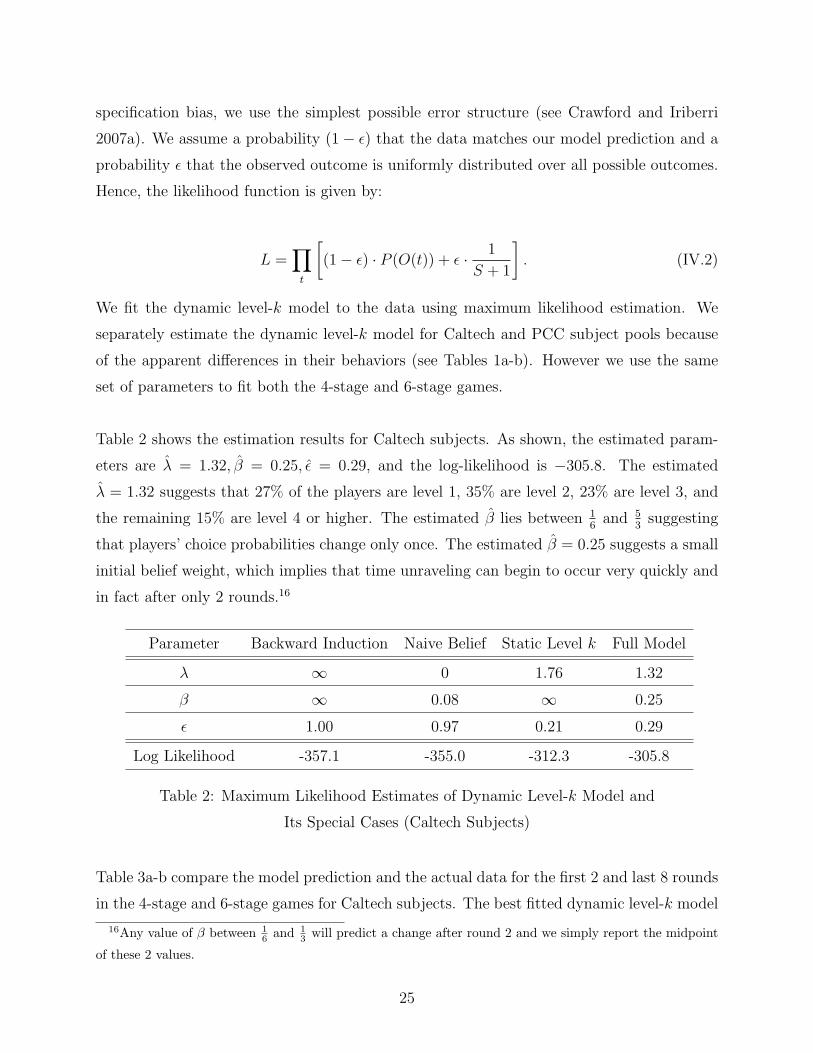
Table 2 shows the estimation results for Caltech subjects. As shown, the estimated param-

eters are λ̂ = 1.32, β̂ = 0.25, ε̂ = 0.29, and the log-likelihood is −305.8. The estimated

λ̂ = 1.32 suggests that 27% of the players are level 1, 35% are level 2, 23% are level 3, and

the remaining 15% are level 4 or higher. The estimated β̂ lies between 16

and 53

suggesting

that players’ choice probabilities change only once. The estimated β̂ = 0.25 suggests a small

initial belief weight, which implies that time unraveling can begin to occur very quickly and

in fact after only 2 rounds.16

Parameter Backward Induction Naive Belief Static Level k Full Model

λ ∞ 0 1.76 1.32

β ∞ 0.08 ∞ 0.25

ε 1.00 0.97 0.21 0.29

Log Likelihood -357.1 -355.0 -312.3 -305.8

Table 2: Maximum Likelihood Estimates of Dynamic Level-k Model and

Its Special Cases (Caltech Subjects)

Table 3a-b compare the model prediction and the actual data for the first 2 and last 8 rounds

in the 4-stage and 6-stage games for Caltech subjects. The best fitted dynamic level-k model

16Any value of β between 16 and 1

3 will predict a change after round 2 and we simply report the midpoint

of these 2 values.

25

makes two predictions. First, in both games, Outcome 0 (i.e., passes all the way) should

not occur in all rounds. Second, the model prescribes that unraveling occurs, and as a

consequence Outcome 1 should not occur after round 2. These predictions were roughly

consistent with the data in the following ways:

1. In both games, Outcome 0 occurs infrequently. For example, Outcome 0 occurs less

than 1% of the time in 6-stage game. The model however fails to capture a nontrivial

proportion of occurrence of outcome 0 in 4-stage game (even though the proportion

declines from 15% to 8% after round 2).

2. In 4-stage game, the proportions of Outcomes 0 and 1 decline after 2 rounds. For

example, the proportion of Outcome 1 decreases from 25% to 11%. In 6-stage game,

Outcomes 0 and 1 rarely occur after round 2 (about 1% of the time).

Outcome 4 3 2 1 0

Rounds 1-2 Data (N=20) 0 0.35 0.25 0.25 0.15

Prediction (ε = 0) 0.15 0.32 0.36 0.17 0

Rounds 3-10 Data (N=80) 0.08 0.45 0.29 0.11 0.08

Prediction (ε = 0) 0.27 0.52 0.21 0 0

Table 3a: A Comparison of Data and Dynamic Level-k Model Prediction

in 4-stage games (Caltech Subjects)

Outcome 6 5 4 3 2 1 0

Rounds 1-2 Data (N=20) 0 0 0.30 0.25 0.45 0 0

Prediction (ε = 0) 0.01 0.04 0.13 0.29 0.36 0.17 0

Rounds 8-10 Data (N=80) 0.03 0.11 0.41 0.29 0.14 0.01 0.01

Prediction (ε = 0) 0.01 0.06 0.24 0.47 0.21 0 0

Table 3b: A Comparison of Data and Dynamic Level-k Model Prediction

in 6-stage games (Caltech Subjects)

Finally, the error rate is around 29% which is not negligible. We believe the value is at-

tributed to the sharp prediction of the dynamic level-k model that both outcome 0 and 1

26

should not occur after round 2.

We also fit three nested cases of the dynamic level-k model. They are all rejected by the

likelihood ratio test. The backward induction model (i.e., λ = β =∞) yields a log-likelihood

of -357.11, which is strongly rejected in favor of the full model (χ2 = 102.7). The naive belief

model (i.e., λ = 0) (which assumes that all players believe that their opponents will always

pass) yields an estimated β̂ = 0.08 and a log-likelihood of −355.00. The model is again

strongly rejected with a χ2 = 98.5. The static level-k model corresponds to β = ∞. Since

players’ initial belief will persist throughout the game plays, they will always choose the

same rule Lk across rounds. This restriction yields a parameter estimate of λ̂ = 1.76 and

provides a reasonable fit with a log-likelihood of -312.29. However, the static model is also

rejected by the likelihood ratio test (χ2 = 13.1, p < 0.01).

Given the MLE estimates of λ̂ = 1.32, β̂ = 0.25, we can generate the dynamic level-k model’s

predicted frequencies for each of the outcomes. Figure 6 shows the actual and predicted fre-

quencies of each outcome. The top panel shows the results for the 4-stage game and the

bottom panel shows the results for the 6-stage game. Backward induction predicts that

only Outcome 4 in 4-stage game and Outcome 6 in 6-stage game can occur (i.e., Player A

takes immediately). This backward induction prediction is strongly rejected by the data. As

shown, the dynamic-k model does a reasonable job in capturing the uni-modal distribution

of the outcomes. In addition, the dynamic level-k model is able to capture the two most

frequently occurring outcomes. Specifically, the dynamic level-k model correctly predicts

that the two most frequently played outcomes are 2 and 3 in 4-stage game and 3 and 4 in

6-stage game.

We also fit our model to the data obtained from PCC subjects. Table 4 shows the esti-

mation results. The dynamic level-k model yields parameter estimates of λ̂ = 1.30 and

β̂ = 1.67. This estimated initial belief weight β̂ > 53

suggests that unraveling never occurs

(i.e., there is no change in the choice probabilities). Therefore, for PCC subjects, the dy-

namic level-k model delivers identical predictions as the static level-k model (i.e., β = ∞),

which also yields an estimated λ̂ = 1.30. Both the static and dynamic level-k models give a

log-likelihood score of -514.75. In contrast, the backward induction prediction (λ = β =∞)

gives a log-likelihood score of -646.47 and the naive belief model (λ = 0) gives a log-likelihood

27

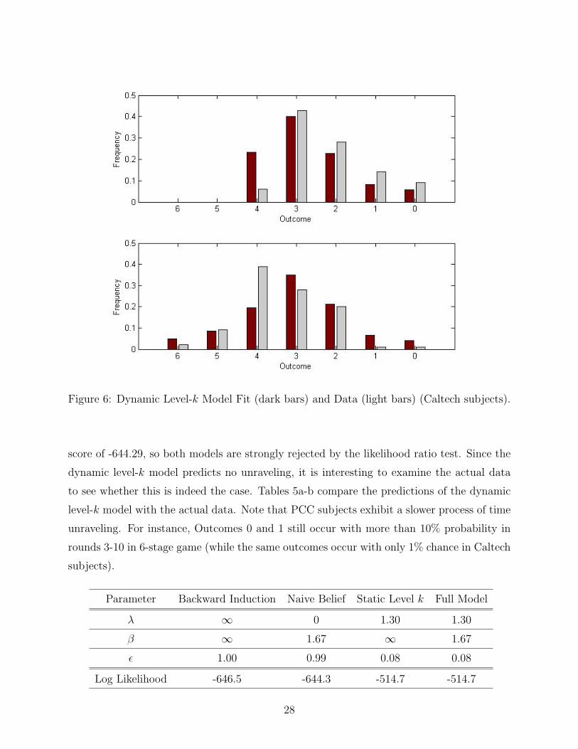
Figure 6: Dynamic Level-k Model Fit (dark bars) and Data (light bars) (Caltech subjects).

score of -644.29, so both models are strongly rejected by the likelihood ratio test. Since the

dynamic level-k model predicts no unraveling, it is interesting to examine the actual data

to see whether this is indeed the case. Tables 5a-b compare the predictions of the dynamic

level-k model with the actual data. Note that PCC subjects exhibit a slower process of time

unraveling. For instance, Outcomes 0 and 1 still occur with more than 10% probability in

rounds 3-10 in 6-stage game (while the same outcomes occur with only 1% chance in Caltech

subjects).

Parameter Backward Induction Naive Belief Static Level k Full Model

λ ∞ 0 1.30 1.30

β ∞ 1.67 ∞ 1.67

ε 1.00 0.99 0.08 0.08

Log Likelihood -646.5 -644.3 -514.7 -514.7

28

Table 4: Maximum Likelihood Estimates of Dynamic Level-k Model and

Its Special Cases (PCC Subjects)

Outcome 4 3 2 1 0

Rounds 1-2 Data (N=38) 0.08 0.24 0.42 0.24 0.03

Prediction (ε = 0) 0.26 0.39 0.27 0.08 0

Rounds 3-10 Data (N=143) 0.08 0.34 0.42 0.14 0.03

Prediction (ε = 0) 0.26 0.39 0.27 0.08 0

Table 5a: A Comparison of Data and Dynamic Level-k Model Prediction

in 4-stage games (PCC Subjects)

Outcome 6 5 4 3 2 1 0

Rounds 1-2 Data (N=38) 0 0.13 0.05 0.32 0.32 0.16 0.03

Prediction (ε = 0) 0.03 0.10 0.20 0.31 0.27 0.08 0

Rounds 8-10 Data (N=143) 0 0.03 0.10 0.48 0.27 0.10 0.01

Prediction (ε = 0) 0.03 0.10 0.20 0.31 0.27 0.08 0

Table 5b: A Comparison of Data and Dynamic Level-k Model Prediction

in 6-stage games (PCC Subjects)

Finally, given the MLE estimates of λ̂ = 1.30, β̂ = 1.67 for PCC subjects, we can generate

the dynamic level-k model’s predicted frequencies for each of the outcomes. Figure 7 shows

the actual and predicted frequencies of each outcome. The top panel shows the results for

the 4-stage game and the bottom panel shows the results for the 6-stage game. The plot

shows that the dynamic level-k model provides a reasonably good fit of the data.

B. Reputation-based Model

As indicated before, backward induction does not admit passing behavior in the centipede

game. To explain why players pass, one can transform the game into a game of incomplete

information by introducing some uncertainty over the player type (Kreps et al., 1982). If

there is a small fraction θ of players that always pass (the so-called altruists), then even

the self-interested players may find it in their best interest to pass initially. However, this

29

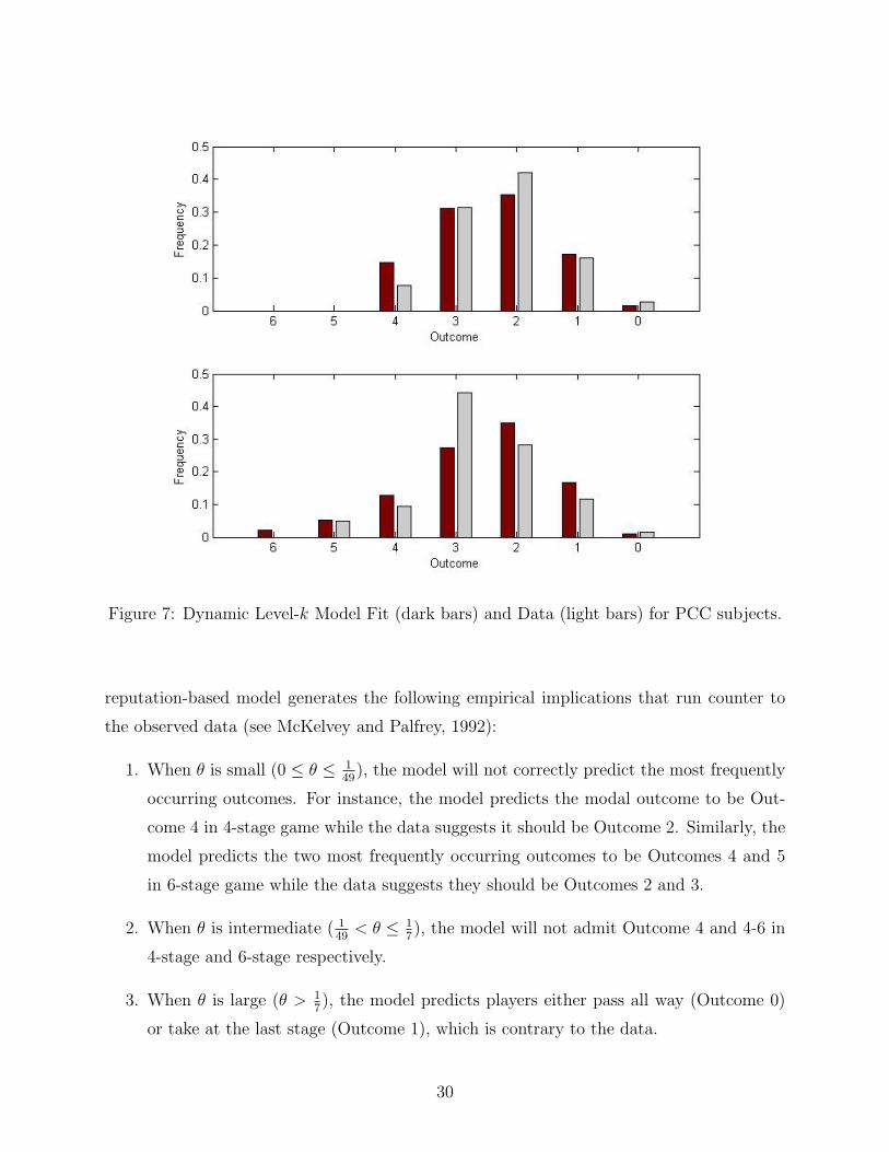
Figure 7: Dynamic Level-k Model Fit (dark bars) and Data (light bars) for PCC subjects.

reputation-based model generates the following empirical implications that run counter to

the observed data (see McKelvey and Palfrey, 1992):

1. When θ is small (0 ≤ θ ≤ 149

), the model will not correctly predict the most frequently

occurring outcomes. For instance, the model predicts the modal outcome to be Out-

come 4 in 4-stage game while the data suggests it should be Outcome 2. Similarly, the

model predicts the two most frequently occurring outcomes to be Outcomes 4 and 5

in 6-stage game while the data suggests they should be Outcomes 2 and 3.

2. When θ is intermediate ( 149< θ ≤ 1

7), the model will not admit Outcome 4 and 4-6 in

4-stage and 6-stage respectively.

3. When θ is large (θ > 17), the model predicts players either pass all way (Outcome 0)

or take at the last stage (Outcome 1), which is contrary to the data.

30

The above discussion suggests that there is not a common θ value that will explain the

unimodal distribution of game outcomes in both the 4-stage and 6-stage games well.

We estimate the reputation-based model using the centipede game data. Like before, we

assume that there is a probability ε that the observed outcome will be evenly distributed

over all possible outcomes. The best fitted model yields θ̂ = 0.050, ε̂ = 0.62 for Caltech

subjects and θ̂ = 0.075, ε̂ = 0.31 for PCC subjects. The log-likelihood scores are -329.80 and

-518.78 respectively, suggesting that the model did a worse job in fitting the data compared

to the dynamic level-k model.

C. Models of Social Preferences

Could the unimodal distribution of game outcomes in centipede game be attributed to social

preferences? The answer is no. To see this we apply the inequity aversion model of Fehr

and Schmidt (1999). Let xi and x−i denote the material payoffs of player i and opponent −irespectively. Then, the payoff of player i, Ui(xi, x−i), is given by:

Ui(xi, x−i) = xi − α · [xi − x−i]+ − β · [x−i − xi]+ (IV.3)

where 0 < α < 1 captures a player’s aversion to being ahead and β > 0 captures a player’s

aversion to being behind. The parameter α is between 0 and 1 because a player who is ahead

will not give up a $1 to benefit her opponent less than $1. One can then solve the game by

backward induction given these revised payoff functions.

Theorem 7 In the centipede game, social preferences lead to either taking immediately or

passing all the way in both the 4-stage and 6-stage games. Specifically, social preferences pre-

dicts that if 3·α−6·β < 2, players will take immediately; otherwise they will pass all the way.

Proof: See Appendix.

The above theorem states that a model of social preferences only admits either Outcome 0

or 4 in 4-stage game and either Outcome 0 or 6 in 6-stage game. The occurrence of either

outcome depends on the fairness parameters α and β. If players are sufficiently averse to

being behind (high β), they will take immediately, which is consistent to backward induc-

tion. On the other hand, if players are sufficiently averse to being ahead (high α), they will

31

pass all the way. Both predictions are inconsistent with the unimodal distribution of actual

game outcomes.

We estimate the social preference model using the centipede game data. Note that the model

fit is identical to the backward induction model. If 3 · α − 6 · β ≤ 2, the model reduces to

backward induction, so the best fit yields a log-likelihood of -357.11 for Caltech subjects and

-646.47 for PCC subjects. If 3 · α − 6 · β ≥ 2, the model predicts that players pass all the

way, so the best fit yields again a log-likelihood of -357.11 and -646.47. Hence the model

perform poorly compared to the dynamic level-k model.

V. Conclusions

In economic experiments, backward induction is frequently violated. We develop a dynamic

level-k model to explain two systematic violations of backward induction. First, players tend

to deviate more from backward induction in games with a greater number of stages or sub-

games. Our model captures this limited induction by allowing players to have heterogeneous

initial beliefs about others’ rationality and hence adopt different rules from a rule hierarchy.

Second, players move closer to backward induction over time. Our model captures this time

unraveling by allowing players to update beliefs of their opponents’ rules and hence adjust

their own rules over time. We show that this adjustment process leads to convergence to-

wards backward induction.

We have applied the dynamic level-k model to 3 canonical games (centipede, finitely repeated

prisoner’s dilemma, and chain store games) that demonstrate the limitations of backward

induction. In all three games, we prove that the limited induction and time unraveling prop-

erties hold. Limited induction holds because the same rule always has a higher deviation

from backward induction in a game with more stages. Time unraveling occurs because the

dynamic level-k model implies a domino effect over time as lower level rules are successively

eliminated.

We fit our model to experimental centipede games of McKelvey and Palfrey (1992). Our

estimation results show that the dynamic level-k model captures the uni-modal distribution

of game outcomes in both 4-stage and 6-stage games reasonably well. Special cases including

32

backward induction and static level-k model are strongly rejected by the data. Interestingly,

Caltech subjects, who are arguably more sophisticated, tend to learn faster than PCC sub-

jects.

We rule out 2 alternative explanations for the observed phenomena in the centipede game.

First, we show that the reputation-based model of Kreps et al. (1982) cannot capture the

uni-modal distribution of game outcomes in the manner consistent with the data. A lim-

itation of the reputation-based model is that there is no common fraction of the altruistic

players that will simultaneously account for the degree of passing in both the 4-stage and

6-stage games. Second, we show that social preferences in the form of inequity aversion (Fehr

and Schmidt 1999) lead to either taking immediately or passing all the way. Consequently, it

cannot explain the uni-modal distribution of game outcomes in both games. Also, a model of

social preferences cannot capture both the limited induction and time unraveling properties.

Our model is a generalization of backward induction. Since the model converges to backward

induction in the limit, it can be conceptualized as a tracing procedure for backward induction,

hence providing a dynamic foundation for backward induction. Framing it this way, the

violations of backward induction in the experiments are simply “transient” behaviors and

our model explicitly characterizes that trajectory.

References

[1] Aumann, R. (1995) ‘Backward Induction and Common Knowledge of Rationality,’

Games and Economic Behavior, 8: 6-19.

[2] Axelrod, R. (1984) The Evolution of Cooperation. Basic Books, Inc. Publishers. New

York.

[3] Bernheim, B. D. (1984) ‘Rationalizable Strategic Behavior’, Econometrica, 52(4): 1007-

1028.

[4] Binmore, K., J. McCarthy, G. Ponti, L. Samuelson and A. Shaked (2002) ‘A Backward

Induction Experiment,’ Journal of Economic Theory, 104: 48-88.

33

[5] Camerer, C. and T-H. Ho (1999) ‘Experience-Weighted Attraction Learning in Normal

Form Games,’ Econometrica, 67: 837-874.

[6] Camerer, C.F., T-H. Ho, J-K. Chong (2004) ‘A Cognitive Hierarchy Model of Games,’

Quarterly Journal of Economics, 119(3): 861-898.

[7] Cooper, R., D. V. DeJong, R. Forsythe, and T. Ross (1996) ‘Cooperation without Repu-

tation: Experimental Evidence from Prisoner’s Dilemma Games,’ Games and Economic

Behavior, 12: 187-218.

[8] Costa-Gomes, M., V. Crawford, and B. Broseta (2001) ‘Cognition and Behavior in

Normal-Form Games: An Experimental Study,’ Econometrica, 69: 1193-1235.

[9] Costa-Gomes, M. and V. Crawford (2006) ‘Cognition and Behavior in Two-Person

Guessing Games: An Experimental Study,’ American Economic Review, 96: 1737-1768.

[10] Costa-Gomes, M., V. Crawford, and N. Iriberri (2009) ‘Comparing Models of Strate-

gic Thinking in Van Huyck, Battalio, and Beil’s Coordination Games,’ Journal of the

European Economic Association, 7: 377-387.

[11] Crawford, V. P. (2003) ‘Lying for Strategic Advantage: Rational and Boundedly Ratio-

nal Misrepresentation of Intentions,’ American Economic Review 93: 133-149.

[12] Crawford, V. and N. Iriberri (2007a) ‘Fatal Attraction: Salience, Naivete, and So-

phistication in Experimental Hide-and-Seek Games,’ American Economic Review, 97:

1731-1750.

[13] Crawford, V. P. and N. Iriberri (2007b) ‘Level-k Auctions: Can a Non-Equilibrium

Model of Strategic Thinking Explain the Winner’s Curse and Overbidding in Private-

Value Auctions?,’ Econometrica, 75: 1721-1770.

[14] Fehr, E. and K.M. Schmidt (1999) ‘A Theory of Fairness, Competition, and Coopera-

tion,’ Quarterly Journal of Economics, 114(3): 81768.

[15] Fudenberg, D. and D. Levine (1998) ‘Theory of Learning in Games,’ Cambridge, MIT

Press.

34

[16] Jung, Y. J., J. H. Kagel, and D. Levin (1994) ‘On the Existence of Predatory Pricing:

An Experimental Study of Reputation and Entry Deterrence in the Chain-Store Game,’

The RAND Journal of Economics, 25(1): 72-93.

[17] Ho, T-H., C. Camerer, and K. Weigelt (1998) ‘Iterated Dominance and Iterated Best

Response in Experimental P-Beauty Contests,’ The American Economic Review, 88:

947-969.

[18] Ho, T-H., C. Camerer, C. and J-K. Chong (2007) ‘Self-tuning Experience-Weighted

Attraction Learning in Games,” Journal of Economic Theory, 133(1): 177-198.

[19] Kreps, D. M., P. Milgrom, J. Roberts, and R. Wilson (1982) ‘Rational Cooperation in

the Finitely Repeated Prisoners’ Dilemma,’ Journal Economic Theory, 27: 245-252.

[20] McKelvey, R. D. and T. R. Palfrey (1992) ‘An Experimental Study of the Centipede

Game,’ Econometrica, 60(4): 803-836.

[21] Palacios-Huerta I. and O. Volijc (forthcoming) ‘Field Centipedes,’ The American Eco-

nomic Review.

[22] Pearce, D. G. (1984) ‘Rationalizable Strategic Behavior and the Problem of Perfection,’

Econometrica, 52(4): 1029-1050.

[23] Reny, P. J. (1992) ‘Backward Induction, Normal Form Perfection and Explicable Equi-

libria,’ Econometrica, 60(3): 627-649.

[24] Rosenthal, R. (1981), ‘Games of Perfect Information, Predatory Pricing, and the Chain

Store,’ Journal of Economic Theory, 25: 92-100.

[25] Selten, R. (1978) ‘The Chain Store Paradox,’ Theory and Decision, 9: 127-159.

[26] Stahl D. and P. Wilson (1995) ‘On Players Models of Other Players - Theory and

Experimental Evidence,’ Games and Economic Behavior, 10: 213-254.

[27] Stahl, D. (1996) ‘Boundedly Rational Rule Learning in a Guessing Game,’ Games and

Economic Behavior, 16: 303-330.

[28] Stahl, D. (2000) ‘Rule Learning in Symmetric Normal-Form Games: Theory and Evi-

dence,’ Games and Economic Behavior, 32: 105-138.

35

Appendix A: Proofs

Proof of Theorem 1 Consider 2 centipede games with s and S subgames, where s < S.

Suppose that the proportion of players who choose each rule level is the same in both games.

Let πk denote the proportion of players who choose rule Lk. Let Eδ(S) denote the expected

deviation in a game with S subgames.

Suppose Player A adopts a level-kA and Player B adopts a level-kB rule in a game with

S stages. Then, the deviation is

δ(LkA, LkB

, S) =1

S

[S −

(min(bkA/2c, S)

2+

min(dkB/2e, S)

2

)],

which is weakly increasing in S for every kA and kB.

Now, comparing the expected deviations in both games, we have

Eδ(S)− Eδ(s) =S∑

kA=1

S∑kB=1

πkAπkB

[δ(LkA, LkB

, S)− δ(LkA, LkB

, s)] ≥ 0,

which gives the required result.

�

Proof of Theorem 2 Consider any player in the centipede game. For concreteness, we

focus on the 4-stage game (see Figure 1) but the proof proceeds in the same way for any

number of stages. Suppose this player holds beliefs B(t) = (b0, b1, . . . , b4) at time t, where

bk denotes this player’s belief of the probability that the opponent will use rule Lk. Let

bkj ≡∑k

i=j bi. Given these beliefs, the player chooses a best-response rule to maximize

expected payoffs.

Let V is denote Player i’s expected payoff, when there are s stages remaining, from fol-

lowing an optimal strategy henceforth. In the last stage, Player B always takes regardless

of beliefs since taking yields 32 a payoff of but passing yields only a payoff of 16. There-

fore, V B1 = 32. In the second-last stage, Player A’s expected payoff is 16 from taking and

64b0 + 8(1− b0) from passing (because after passing, Player B will pass again if and only if

level-0 rule is used, which occurs with probability b0). Thus, V A2 = max{16, 64b0 +8(1− b0)}

and Player A takes if and only if b0 ≤ 1/7. Similarly, in the third-last stage, Player B’s

expected payoff is 8 from taking and V B1 b1

0 + 4(1 − b10) = 32b1

0 + 4(1 − b10) from passing,

so V B3 = max{8, 32b1

0 + 4(1 − b10)} and Player B takes if and only if b1

0 ≤ 1/7. Finally,

36

in the first stage of the 4-stage game, Player A’s expected payoff is 4 from taking and

V A2 b2

0 + 2(1 − b20) from passing. Note that if b2

0 ≤ 1/7, we must have b0 ≤ b20 ≤ 1/7 and

V A2 = 16, so V A

2 b20 + 2(1 − b2

0) ≤ 4 and Player A takes; but if b20 ≥ 1/7, we must have

V A2 b2

0 + 2(1− b20) ≥ 16b2

0 + 2(1− b20) ≥ 4 so Player A passes. Therefore, Player A takes if

and only if b20 ≤ 1/7. Applying this logic, observe that in the s-th last stage of the centipede

game (where s ≥ 2), the player will take if and only if bs−20 ≤ 1/7. Therefore, given beliefs

B(t) = (b0, b1, . . . , b4), the best response rule Lk∗ must be such that k∗ is the largest integer

satisfying bk∗−2

0 ≤ 1/7.

In the model, each player starts at t = 0 with a belief weight of β on some k and adds

a unit weight at each round t. Note that no player will choose L0, so the weights will be

added to levels k ≥ 1 in each round. Therefore, at every t ≥ 6β, we must have b0 ≤ 1/7.

In other words, after round t = 6β, no player will choose L0 or L1, so the weights will

be added to levels k ≥ 2 in subsequent rounds. Similarly, after another 6 · 7β rounds, at

every t ≥ (6 + 6 · 7)β, we must have b10 ≤ 1/7. Continuing with this logic, note that at

every t ≥ (7k − 1)β, we must have bk−10 ≤ 1/7. Therefore, in a S-stage game, at every

t ≥ (7S−1 − 1)β, we have bS−20 ≤ 1/7, so all players use LS = L∞.

�

Proof of Theorem 3 Consider 2 repeated prisoner’s dilemma games with s and S repe-

titions, where ∆ ≡ S − s > 0. Suppose that the proportion of players who choose each rule

level is the same in both games. Let πk denote the proportion of players who choose rule

Lk. Let Eδ(S) denote the expected deviation in a game with S repetitions.

Suppose the players adopt rules of levels k1 and k2. Denote k = max(k1, k2) and k =

min(k1, k2). Then, the deviation is

δ(Lk1 , Lk2 , S) =1

S

[S −min(k, S) +

1{k1 6=k2}2

]because mutual cooperation is sustained in the first S−min(k, S) repetitions and one of the

players continues to cooperate in the next round if k1 6= k2.

Next, we consider the above deviation in several special cases. Denote the sets A =

{0, 1, . . . , s− 1}, B = {s, s + 1, . . . , S − 1}, C = {S, S + 1, . . .}. If k1 = k2 ≡ k, we have the

37

following cases:

k ∈ A ⇒ δ(S) =s− k + ∆

s+ ∆, δ(s) =

s− ks

k ∈ B ⇒ δ(S) =s− k + ∆

s+ ∆, δ(s) = 0

k ∈ C ⇒ δ(S) = δ(s) = 0

If k1 6= k2, we have the following cases:

k ∈ A, k ∈ A ⇒ δ(S) =s− k + 1/2 + ∆

s+ ∆, δ(s) =

s− k + 1/2

s

k ∈ A, k ∈ B ⇒ δ(S) =S − k + 1/2

S≥ 1/2

S, δ(s) =

1/2

s

k ∈ A, k ∈ C ⇒ δ(S) =1/2

S, δ(s) =

1/2

sk ∈ B ∪ C ⇒ δ(S) ≥ δ(s) = 0

Finally, we compute the expected deviations in both games. We obtain:

Eδ(S)− Eδ(s) =S∑

k1=1

S∑k2=1

πk1πk2 [δ(Lk1 , Lk2 , S)− δ(Lk1 , Lk2 , s)]

≥∑

k1,k2∈A

πk1πk2 [δ(Lk1 , Lk2 , S)− δ(Lk1 , Lk2 , s)]

+∑

k∈A,k∈B∪C

πk1πk2 [δ(Lk1 , Lk2 , S)− δ(Lk1 , Lk2 , s)]

≥∑

k1,k2∈A

πk1πk2

[s− k + 1{k1 6=k2}/2 + ∆

s+ ∆−s− k + 1{k1 6=k2}/2

s

]

+∑

k∈A,k∈B∪C

πk1πk2

[1/2

S− 1/2

s

]

≥∑

k1,k2∈A

πk1πk2

[s− k + 1{k1 6=k2}/2 + ∆

s+ ∆−s− k + 1{k1 6=k2}/2

s

]

+∑

k1,k2∈A

πk1πk2

[1

S− 1

s

]

=∑

k1,k2∈A

πk1πk2

[s− k + 1{k1 6=k2}/2 + ∆ + 1

s+ ∆−s− k + 1{k1 6=k2}/2 + 1

s

]≥ 0.

The second last inequality holds because Prob{k ∈ A, k ∈ B ∪ C} ≥ 2 · Prob{k1, k2 ∈ A},and the last inequality holds because

s−k+1{k1 6=k2}/2+1

s≤ 1 whenever k1, k2 ∈ A. Therefore,

the expected deviation is higher in a game with more repetitions.

38

�

Proof of Theorem 4 Consider any player in the repeated prisoner’s dilemma with S

repetitions. Suppose this player holds beliefs B(t) = (b0, b1, . . . , bS) at time t, where bk

denotes this player’s belief of the probability that the opponent will use rule Lk. Let bkj ≡∑ki=j bi. Given these beliefs, the player chooses a best-response rule to maximize expected

payoffs.

Let Vs denote the player’s expected continuation payoff from following an optimal strategy

henceforth, when there are s stages remaining and mutual cooperation was sustained for all

previous S − s stages.

In the last repetition, the player always defects (since this is a dominant strategy), so

V1 = 5b0 +1 · (1− b0), since there is a probability of b0 that the opponent will use rule L0 and

cooperate in the last repetition. In general, in the s-th last repetition, the player’s expected

continuation payoff from defecting is Ds ≡ (5 + (s − 1))bs−10 + s(1 − bs−1

0 ) because the

opponent cooperates in this repetition with probability bs−10 and the payoff in all subsequent

repetitions will be 1; similarly, the player’s expected continuation payoff from cooperating

is Cs ≡ (3 + Vs−1)bs−10 + (s − 1)(1 − bs−1

0 ). Therefore, for every value of s, we obtain

Vs = max{Ds, Cs} = max{(5+(s−1))bs−10 +s(1−bs−1

0 ), (3+Vs−1)bs−10 +(s−1)(1−bs−1

0 )}.Next, we show that the intermediate result that Vs+1 − Vs ≥ 1 for every s ≥ 1. To see

this, first, note that V2 − 1 ≥ V1 because V2 − 1 ≥ D2 − 1 = [5b10 + (1 − b1

0)] ≥ V1, so the

statement above holds for s = 1. Second, note that if Vs − Vs−1 ≥ 1, it then follows that

Cs+1 − Cs = [(3 + Vs)bs0 + s(1− bs0)]− [(3 + Vs−1)b

s−10 + (s− 1)(1− bs−1

0 )]

≥ [(3 + Vs)bs−10 + s(1− bs−1

0 )]− [(3 + Vs−1)bs−10 + (s− 1)(1− bs−1

0 )]

= [(Vs − Vs−1)bs−10 + (1− bs−1

0 )]

≥ 1,

where the first inequality above holds because 3 + Vs ≥ s. The above result, together with

the fact that Ds+1 −Ds ≥ 1, implies that Vs+1 − Vs ≥ 1. Therefore, by induction, we have

Vs+1 − Vs ≥ 1 for every s ≥ 1. Note that this result implies that Vs − s is increasing in s.

39

When there are s repetitions remaining, the player cooperates if and only if

Cs ≥ Ds

(3 + Vs−1)bs−10 + (s− 1)(1− bs−1

0 ) ≥ (5 + (s− 1))bs−10 + s(1− bs−1

0 )

Vs−1bs−10 ≥ (2 + (s− 1))bs−1

0 + (1− bs−10 )

(Vs−1 − s)bs−10 ≥ 1.

Since both Vs − s and bs0 are increasing in s, the player’s optimal rule given beliefs B(t) =

(b0, b1, . . . , bS) must be Lk∗ , where k∗+1 is the smallest integer s satisfying (Vs−1−s)bs−10 ≥ 1.

In the model, each player starts at t = 0 with a belief weight of β on some k and adds

a unit weight at each round t. Note that no player will choose L0, so the weights will be

added to levels k ≥ 1 in each round. Therefore, at every t ≥ β, we must have b0 ≤ 1/2,

which implies V1 = 5b0 + 1 · (1− b0) ≤ 3 and hence (V1 − 2)b10 ≤ V1 − 2 ≤ 1, so C2 ≤ D2. In

other words, after round t = β, no player will choose L0 or L1, so the weights will be added

to levels k ≥ 2 in subsequent rounds. Similarly, after another 2β rounds, at every t ≥ 3β,

we must have b10 ≤ 1/2. This then implies that V2 = D2 = 6b1

0 + 2(1 − b10) ≤ 4 and hence

(V2 − 3)b20 ≤ V2 − 3 ≤ 1, so C3 ≤ D3 and the player will choose rules with level 3 or higher.

Continuing with this logic, note that at every t ≥ (2k − 1)β, we must have bk−10 ≤ 1/2 and

the player will choose only rules of level k + 1 or higher. Therefore, in a prisoner’s dilemma

with S repetitions, at every t ≥ (2S−1−1)β, we have bS−20 ≤ 1/2, so all players use LS = L∞.

�

Proof of Theorem 5 Consider 2 chain store games with s and S interactions, where

s < S. In each game, assume that the entrants share the same beliefs about the incumbent.

In addition, suppose that the proportion of players who choose each rule level is the same in

both games. Let πk denote the proportion of players who choose rule Lk. Let Eδ(S) denote

the expected deviation in a game with S subgames.

Suppose the incumbent uses rule level kI and the entrants use rule level kE. Then the

deviation is

δ(LkI, LkE

, S) =1

S

{[S − kE]+ +

[min(kE, S)−min(kI , S)]+

2

}.

This is because given the above rules, the entrant chooses to stay out in the first [S − kE]+

interactions, and if kE > kI the incumbent will fight and the entrant will enter for the next

[min(kE, S)−min(kI , S)] rounds.

40

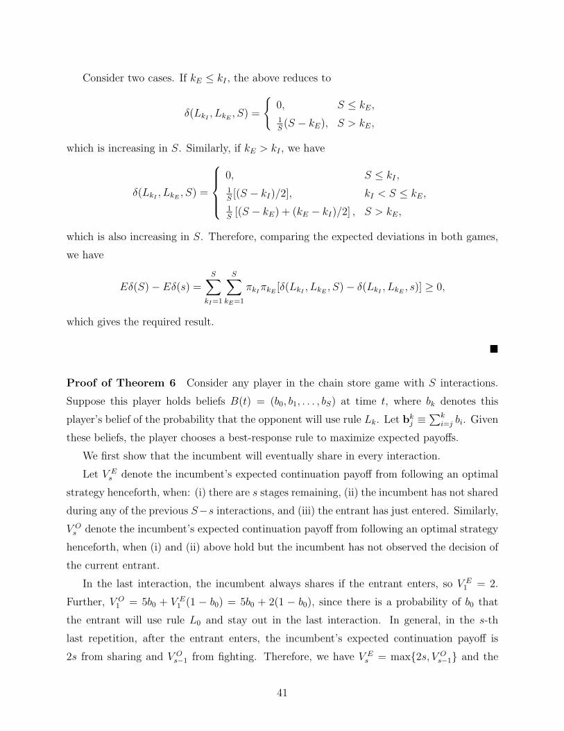
Consider two cases. If kE ≤ kI , the above reduces to

δ(LkI, LkE

, S) =

{0, S ≤ kE,

1S

(S − kE), S > kE,

which is increasing in S. Similarly, if kE > kI , we have

δ(LkI, LkE

, S) =

0, S ≤ kI ,

1S

[(S − kI)/2], kI < S ≤ kE,

1S

[(S − kE) + (kE − kI)/2] , S > kE,

which is also increasing in S. Therefore, comparing the expected deviations in both games,

we have

Eδ(S)− Eδ(s) =S∑

kI=1

S∑kE=1

πkIπkE

[δ(LkI, LkE

, S)− δ(LkI, LkE

, s)] ≥ 0,

which gives the required result.

�

Proof of Theorem 6 Consider any player in the chain store game with S interactions.

Suppose this player holds beliefs B(t) = (b0, b1, . . . , bS) at time t, where bk denotes this

player’s belief of the probability that the opponent will use rule Lk. Let bkj ≡∑k

i=j bi. Given

these beliefs, the player chooses a best-response rule to maximize expected payoffs.

We first show that the incumbent will eventually share in every interaction.

Let V Es denote the incumbent’s expected continuation payoff from following an optimal

strategy henceforth, when: (i) there are s stages remaining, (ii) the incumbent has not shared

during any of the previous S−s interactions, and (iii) the entrant has just entered. Similarly,

V Os denote the incumbent’s expected continuation payoff from following an optimal strategy

henceforth, when (i) and (ii) above hold but the incumbent has not observed the decision of

the current entrant.

In the last interaction, the incumbent always shares if the entrant enters, so V E1 = 2.

Further, V O1 = 5b0 + V E

1 (1 − b0) = 5b0 + 2(1 − b0), since there is a probability of b0 that

the entrant will use rule L0 and stay out in the last interaction. In general, in the s-th

last repetition, after the entrant enters, the incumbent’s expected continuation payoff is

2s from sharing and V Os−1 from fighting. Therefore, we have V E

s = max{2s, V Os−1} and the

41

incumbent fights with s interactions remaining if and only if V Os−1 ≥ 2s. It also follows that

V Os = (5 + V O

s−1)bs−10 + V E

s (1− bs−10 ).

Next, we show that V Os−1 ≥ 2s implies V O

s ≥ 2(s+ 1) for every s ≥ 2. We first check this

for s = 2: when V O1 − 4 = b0 − 2(1− b0) ≥ 0, we have

V O2 − 6 = [3 + (V O

1 − 4)]b10 + {[V O

1 − 4]+ − 2}(1− b10)

≥ (V O1 − 4) + 3b1

0 − 2(1− b10)

≥ (V O1 − 4) + 3b0 − 2(1− b0) ≥ 0,

as stated. In general, suppose V Os−1 ≥ 2s. Further, suppose V O

t−1 ≥ 2t holds for t = s− 1, s−2, . . . , s− r + 1 but not for t = s− r. Since the above inequality holds for t = s− r + 1 but

not for t = s− r, we know that V Os−r−1 − 2(s− r) < 0 but

V Os−r−2(s−r+1) = [3+(V O

s−r−1−2(s−r))]bs−r−10 +{[V O

s−r−1−2(s−r)]+−2}(1−bs−r−10 ) ≥ 0,

so we must have 3bs−r−10 − 2(1 − bs−r−1

0 ) ≥ 0 and hence 3bs−10 − 2(1 − bs−1

0 ) ≥ 0. Note

that if r = s − 1 above (i.e., V Ot−1 ≥ 2t holds for all t from 2 to s), then we also have

3bs−10 − 2(1− bs−1

0 ) ≥ 3b0 − 2(1− b0) ≥ b0 − 2(1− b0) = V O1 − 4 ≥ 0. Therefore, we obtain

V Os − (s+ 1) = [3 + (V O

s−1 − s)]bs−10 + {[V O

s−1 − s]+ − 2}(1− bs−10 )

≥ (V Os−1 − s) + 3bs−1

0 − 2(1− bs−10 ) ≥ 0,

as stated.

When there are s interactions remaining, the incumbent fights if and only if V Os−1 ≥ 2s.

From the result in the previous paragraph, we know that the incumbent will fight in all

previous interactions if the same applies to the current interaction. Therefore, given beliefs

B(t) = (b0, b1, . . . , bS), the incumbent’s best-response rule must be Lk∗ , where k∗ + 1 is the

smallest integer s satisfying V Os−1 ≥ 2s.

In the model, each incumbent starts at t = 0 with a belief weight of β on some k and

adds a unit weight at each round t. Note that no incumbent will choose L0, so the weights

will be added to levels k ≥ 1 in each round. Therefore, after a finite number of rounds, we

must have b0 ≤ 2/3, which implies V O1 − 4 = b0 − 2 · (1 − b0) ≤ 0. In other words, after a

finite number of rounds, the incumbent will never choose L0 or L1, so the weights will be

added to levels k ≥ 2 in all subsequent rounds. Similarly, after another finite number of

rounds, we must have b10 ≤ 2/5. This then implies that V O

2 ≤ 3b10 − 2(1 − b1

0) ≤ 0, so the

42

incumbent will choose rules with level 3 or higher subsequently. Continuing with this logic,

note that for every k, after a finite number of rounds, we must have bk−10 ≤ 2/5 and the

incumbent will choose only rules of level k + 1 or higher. Therefore, in a chain store game

with S interactions, after a finite number of rounds, we have bS−20 ≤ 2/5, so the incumbent

will use LS = L∞ subsequently.

Finally, we show that the entrant will eventually share in every interaction. Consider an

entrant that is followed by s subsequent entrants. This entrant’s expected payoff is 1 from

staying out and 2(1−bs0) from entering. Thus, this entrant will enter if and only if bs0 ≤ 1/2.

Following the same logic above, note that for every s, we will eventually have bs0 ≤ 1/2 after

a finite number of rounds. Therefore, in a chain store game with S interactions, the entrant

will eventually enter at every interaction.

�

Proof of Theorem 7 We will prove the result for a 4-stage game. The proof for a 6-stage

game proceeds similarly. First, consider the case where 3α − 6β ≤ 2. In the last stage, the

payoffs to Players A and B respectively are (8,32) if Player B takes and (64,16) if Player

B passes. The corresponding utilities to Player B are 32 − 24α and 16 − 48β respectively.

Since the condition 3α − 6β ≤ 2 holds, Player B prefers to take. Reasoning backwards, in

the second last stage, the payoffs to both players are (16,4) if Player A takes and (8,32) if

Player A passes (since Player B will then take in the last stage). The corresponding utilities

to Player A are 16−12α and 8−24β, so by the same condition above, Player A takes. Using

the same reasoning, players will take in every stage.

Next, consider the other case where 3α − 6β ≥ 2. By the calculations above, we know

that Player B will now pass in the last stage. Now, in the second last stage, the payoffs to

Players A and B are (16,4) if Player A takes and (64,16) if Player A passes (since Player

B will also pass in the last stage). The utilities are 16 − 12α and 64 − 48α. Since α ≤ 1,

the latter is greater and thus Player A passes. Proceeding backwards, in the third last stage

(i.e., Stage II), Player B’s payoff from taking is 8−6α, which is less than his payoff 32−24α

from taking in the last stage, because α ≤ 1. Since Player B prefers passing in the last stage,

the same applies in this stage as all players will pass subsequently. Using the same logic,

players will pass in every stage.

�

43