A distillate composition estimator for an industrial multicomponent IC4-NC4 splitter with experimental temperature measurements

Marcella Porru*, Jesus Alvarez**

Roberto Baratti*

* Dip. Ingegneria Meccanica, Chimica e dei Materiali, via Marengo, 2 09123 Cagliari, Italy.

** Dep. de Ingeniería de Procesos e Hidráulica, UAM, Apdo. 55534, 09340 México, D.F. Mexico

Abstract: The problem of on-line estimating on the basis of temperature measurements the distillate NC4 impurity in an industrial IC4-NC4 splitter is addressed within an adjustable-structure Geometric Estimation approach, yielding: (i) suggestive sensor location guidelines drawn from detectability measures, and (ii) conclusive results obtained from estimator functioning assessment with simulated and experimental data. The resulting estimator performs the estimation task within an admissible error tolerance, and considerably less ODEs than the ones of the standard EKF technique employed in the majority of related previous studies.

Keywords: multicomponent distillation column, estimation structure, geometric estimator.

1. INTRODUCTION

Distillation columns are important energy-consuming industrial units where a mixture is separated into two or more key components. The related control problem consists in efficiently performing the component separation in the presence of disturbances, in the sense of purity within prescribed limits, and non-wasteful control action. Due to high investment and maintenance costs as well as equipment reliability and measurement delay problems of on-line composition analyzers, more often than not an effluent composition controller cannot be implemented. This motivates the development of (first-principle or empirical) model-based composition estimators driven by temperature measurements for monitoring and control purposes.

Basically, this estimation problem has been addressed with the first-principle (mostly EKF) (Baratti et al., 1998) and (input-output) data driven (Mejdell and Skogestad, 1993) models. The EKF functions rather well over an ample set of column types and operating condition, but its implementation requires a detailed first-principle model and the on-line integration of a number of ODEs that grows rapidly (quadratically) with the number of stages and components. The data driven approach does not require a first-principle model, but its implementation requires intensive model identification effort with experimental input-output data, and its validity is restricted to a specific column operating condition.

Recently, the dimensionality problem of the model based EKF approach for multicomponent distillation column (Frau et al, 2010) has been addressed with the so-called Geometric Estimation (GE) approach (Álvarez and Fernandéz, 2009).

While in the EKF a complete observability is required and the model is fixed, in the GE only detectability is needed and the (possibly truncated) model is a design degree of freedom. The GE has been successfully implemented in binary laboratory (Fernandez et al., 2012) and ternary pilot (Pulis, 2007) columns with experimental data, and tested with a six-component industrial scale column through simulations (Frau et al., 2010). In the present study, the implementation with industrial experimental data of a geometric estimator is presented for a multicomponent industrial (IC4-NC4 splitter) column.

Specifically, in this paper the problem of on-line estimating the distillate NC4 impurity for an industrial IC4-NC4 splitter (operating at Saras refinery at Sarroch in Italy) on the basis of temperature measurements is addressed. The estimator design includes decisions on the number of modeled components, the innovated component (where the measurement information is injected) as well as on the number of sensors and their locations. The problem is addressed with a GE framework (Álvarez, 2000) through sensitivity measures drown from staged detectability considerations (Fernandez et al., 2012; Frau et al., 2010), sensitivity-based measurement location arguments for column control (Luyben, 2006), and the analysis of the steady state per-component temperature gradient diagram for structure design in multicomponent distillation column (Frau et al., 2010). For applicability purposes, we are interested in an estimation algorithm which guarantees a trade-off between robustness, state reconstruction speed, and simplicity in terms of number of first-principle equations that is considerably smaller than the ones of the EKF employed in the majority of previous multicomponent distillation column studies (Baratti et al., 1998).

Preprints of the 10th IFAC International Symposium on Dynamics and Control of Process SystemsThe International Federation of Automatic ControlDecember 18-20, 2013. Mumbai, India

Copyright © 2013 IFAC 391

2. ESTIMATION PROBLEM

2.1 IC4-NC4 splitter

Consider the industrial heptacomponent distillation column located at Saras refinery (Sarroch, Italy) and depicted in Fig. 1, where iso-butane (IC4) and normal-butane (NC4) splitting occurs. Since the distillate is fed to a subsequent alkylation reactor to produce high-octane gasoline, the distillate must contain mostly IC4 accompanied by a prescribed small amount of NC4. The column has 57 stages, three kettle reboilers (1-th stage), total condenser (57-th stage), temperature measurement at 49-th stage, and feed at the 33-th stage made of a mixture of paraffins with olefins. Nominal component composition and normal boiling point are listed in Table 1.

Fig. 1. The splitter IC4-NC4.

Table 1. Hydrocarbons and their nominal compositions and normal boiling points in the splitter feed.

Feed composition

[molar fraction]

Normal boiling point [K]

Propane C3 0.008 231.1 I-butane IC4 0.394 261.4 I-butene IC4- 0.032 266.2 N-butene NC4- 0.031 266.9 N-butane NC4 0.467 272.7

2-butene trans C4-T 0.039 274.0 2-butene cis C4-C 0.029 276.9

The column has a PI temperature controller that adjusts the reboiler heat injection rate on the basis of the temperature sensor in 49-th stage of the enrichment section in order to maintain the heavy key component (NC4) distillate molar fraction above (or below) the low (or high) limit 0.01 (or 0.06).

From standard assumption (Baratti et al., 1998) (material balances, energy balance neglected on each tray, feed variation due to feed and reflux subcoolings only, tight

controller and condenser level control, and ideal vapor-liquid equilibrium) the N-stage C-component m-measurement close loop column dynamics are described by the dynamical system (1):

),,( dxfx PPP u= , )( Pp xhy = (1a,b)

343111 =+−=+= )()dim( CNnPPx , m=)dim(y where

TTN

T ],...,[ ccxP 1= , ],...,[ 11 −= Ciii ccc

are the state vector, and the composition vector at i-th stage;

Vu = , TTFF ],[ cd = ,

sTy =

are respectively, the input, the exogenous disturbance and the output. V (or F) is the vapor (or feed) flow rate;

TmTT ],...,[ 1=sT , ],...,[ 11 −= C

FFF ccc

are the m-dimensional vector of temperature measurements, and the feed composition vector;

)](),...,([ mPP cchP ββ 1= is the output map, and βP is the bubble point function. The thermodynamics (liquid-vapor equilibrium and bubble point functions) are set with the 5-parameter Wagner equation (Reid et al., 1988). The steady state (SS) temperature and composition profiles are presented in Fig. 2 showing that: (i) no high purity separation occurs between IC4-NC4 key components, (ii) the global butylen composition is not negligible through the column, and (iii) since their similar thermodynamic properties and profile behaviors, the light (or heavy) butylens and IC4- and NC4- (or C4-C and C4-T) can be depicted as a single pseudo component.

Fig. 2. SS temperature and composition profiles.

2.2 Experimental data

In Fig. 3 are presented the industrial column data for estimator implementation: (i) total (3.a) and olefin (3.b) feeds, (ii) distillate (3.c), (iii) reflux (3.d) flows, and (iv)

IFAC DYCOPS 2013December 18-20, 2013. Mumbai, India

392

output temperature measurement at 49-th stage (3.e). Since the olefin (and paraffin) feed nominal composition is available from discrete-delayed offline chromatographic determination, butylen (and paraffin) compositions in the total feed can be approximately calculated time by time from a mass balance applied in the node N (see Fig. 1), where the blending occurs. The estimator must be tested with the actual temperature sensor location (stage 49).

In Fig. 4 are presented the distillate NC4 experimental concentration data, with chromatographic analysis approximately every 15 minutes, in the understanding that these data will be used for estimator functioning assessment and not for estimator implementation.

Fig. 3. Input-output industrial data for estimator implementation.

Fig. 4. Industrial data for estimator functioning assessment: NC4 distillate molar fraction.

2.3 Estimation problem

Since the control objective is to maintain the NC4 distillate composition within prescribed low (0.01) and high (0.06) limit values, it suffices to estimate the NC4 composition within a reasonable uncertainty (to be determined). Thus, the estimation problem consist in designing: (i) the structure (number of modeled and innovated components as well as the number of sensors and their location) on the basis of the detailed column dynamics (1), and (ii) the on-line estimation algorithm with a simplified model (to be designed), in such a way that the estimator has less ODEs than the ones of the EKF. The estimator must be tested with the experimental data (Fig. 3) and compared with the concentration data (Fig. 4). The pertinence of relocating and adding measurements or not must be assessed.

3. ADJUSTABLE-STRUCTURE ESTIMATION

In this section the column estimation problem is casted as an estimation structure design problem within a Geometric Estimation framework (Álvarez and Fernandéz, 2009) for staged systems (Fernandez et al., 2012), in the understanding that the estimation algorithm is uniquely determined by the estimation structure. For this aim, structure selection guidelines are drawn from detectability considerations in the light of: (i) the per-component temperature gradient (PCTG) diagram for sensor location in multicomponent estimation (Frau et al., 2010), and (ii) sensitivity-like measurement location criteria employed in previous estimation (Frau et al., 2010; Fernandez et al., 2012), and control (Luyben, 2006) studies.

3.1 Detectable model set

By virtue of the staged feature of the column (Fernandez et al., 2012), the multisensor detectability assessment can be performed using a single-sensor single-innovation model with the complete (C-component) model (1). For the purpose at hand, let us introduce the robust detectability structure (Fernandez et al., 2012) σd ={i, Cj, µ} ∈ Σd, Cj ∈ µ = {C1, … CCM} (2a) where i : sensor location, Cj: innovated component, µ: modeled component set, Σ d : structure set. and the robust detectability condition

Dii cabs εβ ι ≥∂∂ ))(( c (2b) ciι is the composition of Cj at stage i and ci is the composition

of C1,…,CCM-1 at stage i. The associated set of detectable estimation models (one per structure σd) is given by:

),,,( dx uxfx νιιι = ; )( ihy c= , ],[ ιυiii ccc = (3a,b)

),,,( dxfx ux νινν = , 111 +=+−= MnCMN )()dim(x (3c)

1== )dim()dim( yxι , 1−= Mn)dim( νx

where xι (or xυ) is the innovated (or noninnovated) 1 [or (nM-1)]-dimensional state, CM is the number of modeled components, i is the measurement stage, ci

ι (or ciυ) is the [1

(or CM-1)]-dimensional innovated (or noninnovated) composition at the measurement stage i. The corresponding indistinguishable (kind of unobservable) stable dynamics are given by

),,(:),,,),(( dxfdxcfx uuyh Ii ννν

νν == −1 (4a)

),(),( yhyhx Ii νν

ι xc == −1 (4b)

where h-1 denotes the robust solution (by virtue of the detectability condition 2b) for the innovated state xι of the algebraic output equation (4b). From the stability of the (nM+1)-dimensional column model (2) and the robust invertibility (4b) of the output map (3b) the stability of the indistinguishable (nM-1)-dimensional dynamics (4a) follows.

IFAC DYCOPS 2013December 18-20, 2013. Mumbai, India

393

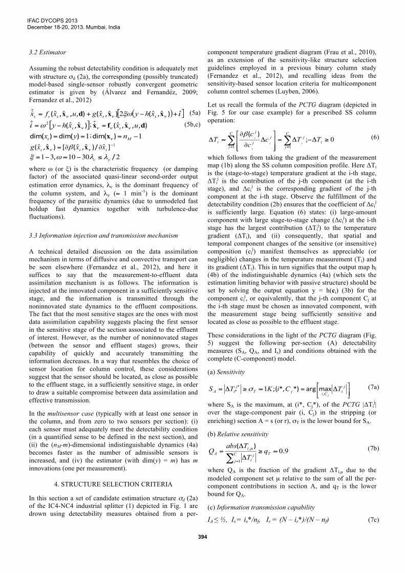
3.2 Estimator

Assuming the robust detectability condition is adequately met with structure σd (2a), the corresponding (possibly truncated) model-based single-sensor robustly convergent geometric estimator is given by (Álvarez and Fernandéz, 2009; Fernandez et al., 2012)

( )[ ]ιξω νινινιιι ˆ)ˆ,ˆ()ˆ,ˆ(),,ˆ,ˆ(ˆ +−+= xxdx xhyxguxfx 2 (5a)

[ ])ˆ,ˆ(ˆνιωι xxhy−= 2 ; ),,ˆ,ˆ(ˆ dxfx ux νινν = (5b,c)

1== )dim()dim( yxι ; 1−= Mn)dim( νx 1−∂∂= ]ˆ/)ˆ,ˆ([)ˆ,ˆ( ινινι β xxxg xx 2301031 /, yc λλωξ ≤−≈−=

where ω (or ξ) is the characteristic frequency (or damping factor) of the associated quasi-linear second-order output estimation error dynamics, λc is the dominant frequency of the column system, and λy (≈ 1 min-1) is the dominant frequency of the parasitic dynamics (due to unmodeled fast holdup fast dynamics together with turbulence-due fluctuations).

3.3 Information injection and transmission mechanism

A technical detailed discussion on the data assimilation mechanism in terms of diffusive and convective transport can be seen elsewhere (Fernandez et al., 2012), and here it suffices to say that the measurement-to-effluent data assimilation mechanism is as follows. The information is injected at the innovated component in a sufficiently sensitive stage, and the information is transmitted through the noninnovated state dynamics to the effluent compositions. The fact that the most sensitive stages are the ones with most data assimilation capability suggests placing the first sensor in the sensitive stage of the section associated to the effluent of interest. However, as the number of noninnovated stages (between the sensor and effluent stages) grows, their capability of quickly and accurately transmitting the information decreases. In a way that resembles the choice of sensor location for column control, these considerations suggest that the sensor should be located, as close as possible to the effluent stage, in a sufficiently sensitive stage, in order to draw a suitable compromise between data assimilation and effective transmission.

In the multisensor case (typically with at least one sensor in the column, and from zero to two sensors per section): (i) each sensor must adequately meet the detectability condition (in a quantified sense to be defined in the next section), and (ii) the (nM-m)-dimensional indistinguishable dynamics (4a) becomes faster as the number of admissible sensors is increased, and (iv) the estimator (with dim(y) = m) has m innovations (one per measurement).

4. STRUCTURE SELECTION CRITERIA

In this section a set of candidate estimation structure σd (2a) of the IC4-NC4 industrial splitter (1) depicted in Fig. 1 are drown using detectability measures obtained from a per-

component temperature gradient diagram (Frau et al., 2010), as an extension of the sensitivity-like structure selection guidelines employed in a previous binary column study (Fernandez et al., 2012), and recalling ideas from the sensitivity-based sensor location criteria for multicomponent column control schemes (Luyben, 2006).

Let us recall the formula of the PCTG diagram (depicted in Fig. 5 for our case example) for a prescribed SS column operation:

011

≥Δ−Δ=⎥⎥⎦

⎤

⎢⎢⎣

⎡Δ

∂

∂≈Δ ∑∑

==i

C

j

jC

j

jj

j

i TTccc

Tii

i

i ;)(β (6)

which follows from taking the gradient of the measurement map (1b) along the SS column composition profile. Here ΔTi is the (stage-to-stage) temperature gradient at the i-th stage, ΔTi

j is the contribution of the j-th component (at the i-th stage), and Δci

j is the corresponding gradient of the j-th component at the i-th stage. Observe the fulfillment of the detectability condition (2b) ensures that the coefficient of Δci

j is sufficiently large. Equation (6) states: (i) large-amount component with large stage-to-stage change (Δci

j) at the i-th stage has the largest contribution (ΔTi

j) to the temperature gradient (ΔTi), and (ii) consequently, that spatial and temporal component changes of the sensitive (or insensitive) composition (ci

j) manifest themselves as appreciable (or negligible) changes in the temperature measurement (Ti) and its gradient (ΔTi). This in turn signifies that the output map hI (4b) of the indistinguishable dynamics (4a) (which sets the estimation limiting behavior with passive structure) should be set by solving the output equation y = h(ci) (3b) for the component ci

j, or equivalently, that the j-th component Cj at the i-th stage must be chosen as innovated component, with the measurement stage being sufficiently sensitive and located as close as possible to the effluent stage.

These considerations in the light of the PCTG diagram (Fig. 5) suggest the following per-section (A) detectability measures (SA, QA, and Is) and conditions obtained with the complete (C-component) model.

(a) Sensitivity

⎥⎦⎤

⎢⎣⎡ Δ=≈≥Δ= j

iCijTjiA TCiKTS

j,

** maxarg*)*,(;1σ (7a)

where SA is the maximum, at (i*, Cj*), of the PCTG |ΔTij|

over the stage-component pair (i, Cj) in the stripping (or enriching) section A = s (or r), σT is the lower bound for SA.

(b) Relative sensitivity

901

.)( , ≈≥

Δ

Δ=∑ =

TC

jji

iA q

T

TabsQ µ (7b)

where QA is the fraction of the gradient ΔTi,µ due to the modeled component set µ relative to the sum of all the per-component contributions in section A, and qT is the lower bound for QA.

(c) Information transmission capability

IA ≤ ½, Is = is*/nf, Ir = (N – ir*)/(N – nf) (7c)

IFAC DYCOPS 2013December 18-20, 2013. Mumbai, India

394

where IA is the fraction of the sensor location-to-effluent stages is* (or N – ir*) in the stripping (or enriching) section A = s (or r) referred to the number of stages nf (or N – nf) in the same section, being nf the feed stage.

The per-section single-sensor structure which meets the preceding conditions is called admissible structure and is denoted by

σ ={σs, σr} ∈ Σ2, σA ={iA, Cj, µ} ∈ Σ1, A=s,r (8) if the conditions (7a) are not met at section A = s (stripping) or r (rectifying), the structure of section A is denoted by

σA = σA ν ={iA = ∅, Cj, µ} meaning that a sensor is not placed in section A, and the estimation of compositions is performed with the noninnovated dynamics (5c) of section A. In the same way, a per-section structure for more than one sensor can be considered.

Fig. 5. Per-component temperature gradient and global gradient diagram.

4.1 Structure selection guidelines

For a given (single or two effluent) estimation objective, the aim of the structure selection procedure is to draw an adequate estimator functioning in the sense of a suitable compromise between reconstruction speed and accuracy, asymptotic offset, robustness with respect to exogenous disturbances, modeling errors, and sensor locations, as well as estimation algorithm simplicity (in terms of number of ODEs and their conditioning). The preceding considerations suggest the structure selection guidelines.

1. On the basis of the complete (C-component) model, plot the component, temperature and PCTG diagrams. Identify the key and non-key components, as it is done in column design and control schemes (Luyben, 2006).

2. Identify the sensitive stage (is* and ir*) and component (Cjs* and Cjr*) in each section, and the corresponding

modeled component set µ*. Draw the candidate one or two-sensor structure

σ∗ ={σs*, σr*} ∈ Σ2, σA* ={iA*, Cj*, µ∗} ∈ Σ1 (9) which meet the sensitivity and transmission conditions (7).

3. Verify with simulation and/or experimental implementation the functioning of this structure, and perform “structural tuning” by adjusting the sensor locations, the modeled component set (µ), and adding more sensors.

4.2 Candidate structures

The application of the preceding guidelines in the light of the temperature, composition (Fig. 2) and PCTG (Fig. 5) diagram: (i) shows that the column splitter has rather poor sensitivity in the stripping section and closed-to-low limit sensitivity in the rectifying section, according to the detectability measures,

(Ss, Qs, Is) ≈(1.25, 0.93,1), (Sr, Qr, Ir) ≈(1.35, 0.94, 0.5) this suggests the consideration of the single-sensor two-component candidate structure

σ1 ={ ir = 44, Cj = IC4, µ}, µ = {IC4, NC4} (10) without sensor in the insufficiently sensitive stripping section. The fact that the industrial experimental data were generated with a single sensor located at stage 49 leads us to consider the “neighboring” candidate two and three-modeled component structures

σ2 ={ ir = 49, Cj = IC4, µ}, µ = {IC4, NC4} (11) (Sr, Qr, Ir)2 ≈ (1.21,0.90,0.3) σ3 ={ ir = 49, Cj = IC4, µ}, µ = {IC4,NC4,NC4-} (12) (Sr, Qr, Ir)2 ≈ (1.21,0.94,0.3) drawn with the following rationale. Due to the 5 stage movement of the location towards the column top, in the passage from the two-component (IC4-NC4) structure σ1 to σ2, there is a loss (or gain) of information injection (or transmission) capability. The presence of a larger amount of no-key components in stage 49 suggests that the gain of binary model-based information transmission capability should be lost to some appreciable extent. To compensate this loss, a third component (NC4- as lump of NC4 and IC4) is added to the column, yielding the candidate structure σ3.

5. STRUCTURAL RESULTS

Having as point of departure the suggestive structural results of the previous section, in this section conclusive structural results are obtained through simulation and implementation with experimental data.

The application of the tuning guidelines with implementation testing over the three structures yielded the estimator damping (ξ) and frequency (ω) values ξ = 1.5, ω = 15 h-1 ≈ 10 λc > λy = 0.05 h-1.

First, the three estimator structures σ1, σ2 and σ3 were implemented whit estimators driven by the temperature generated with a numerical simulation of the complete (7-

IFAC DYCOPS 2013December 18-20, 2013. Mumbai, India

395

component) column model (1). The corresponding results are presented in Fig. 6, showing that structure σ3 yields the best behavior followed by structure σ1 and σ2. The ternary model-based structure σ3 functioned well with any sensor location in the stage interval 43-49. Comparing with structure σ1 (binary model and measurement at stage 44) the mild behavior degradation of structure σ2 (binary model and measurement at stage 49) is due to the change in sensor location. Thus, the ternary model-based structure σ3 is less sensitive to the sensor location than its binary model-based counterpart.

Fig. 6. Simulation-based complete model (dotted line) (1),

and estimator functioning for structures σ1 (continuous line) (10), σ2 (dot-dashed line) (11) and σ3 (dashed line) (12)

In Fig. 7 is presented the estimator functioning with the structure σ2 and σ3 and experimental data (on-line temperature sensor at stage 49), including comparison with experimental (chromatographic) off-line NC4 composition data and showing that the ternary model-based structure σ3 outperform its binary model-based counterpart structure σ2. In others words structure σ3 is more tolerant to the sensor location deviation than structure σ1. Basically, these experimental results are in agreement with the ones obtained with theoretical arguments and numerical simulations.

According to Fig. 7, the ternary model-based estimator, without any adjustment of thermodynamic parameters, yields a ≈ 4% average offset error, which is acceptable for the present column. Should this error be larger or unacceptable, the offset error can be reduced through model calibration on the basis of the occasional (typically discrete-delayed) distillate composition determination that are commonly performed for process monitoring processing.

Fig. 7. Estimator functioning with experimental temperature

measurement (stage 49) for structures: σ2 (dashed line) (11) and σ3 (continuous line) (12), and comparison with experimental (dotted line) distillate NC4 composition.

6. CONCLUSIONS

The problem of online estimating the distillate NC4 impurity of an industrial IC4-NC4 splitter has been addressed within a GE framework. First, candidate structures were drawn from the examination of the PCTG diagram in the light of detectability measures. Then, conclusive results were obtained through simulation and experimental industrial data: the estimation task can be adequately performed with a ternary model, with robustness with respect to sensor location and modeling errors. The implementation of this estimator requires the on-line integration of 115 ODEs, which are considerably less than the ones (6670) of its conventional EKF counterpart. It must be pointed out that a closely similar behavior can be attained using a binary model with sensor at the most sensitive stage in the rectifying section, with an unacceptable cost of behavior with sensor location changes. This study should constitute a point of departure to study the incorporation of discrete-delayed composition measurements, and the connection between sensor location criteria for estimation and control.

ACKNOWLEDGEMENT

M. Porru thankfully acknowledges SARAS refinery for the fellowship support.

REFERENCES

Álvarez, J. (2000). Nonlinear state estimation with robust convergence. Journal of Process Control, 10, 59-71.

Álvarez, J., Fernandéz, C. (2009). Geometric estimation of nonlinear process systems. Journal of Process Control, 19, 247-260

Baratti, R., Da Rold, A., Bertucco, A., and Morbidelli, M. (1998). A composition estimator for multicomponent distillation columns - development and experimental test on ternary mixtures. Chemical Engineering Science, 53, 20, 3601-3612.

Fernandéz, C., Álvarez, J., Baratti, R., Frau, A. (2012) Estimator structure design for staged systems. Journal of Process Control, 22, 2038-2056.

Frau, A., Baratti, R., Álvarez, J. (2010). Measurement structure design for multicomponent distillation column with specific estimation objective. In IFAC-ADCHEM 2010, 784-792.

Luyben, W.L. (2006) Evaluation of criteria for selecting temperature control trays in distillation columns, Journal of Process Control, 16, 115–134

Mejdell, T., Skogestad, S. (1993). Output estimation using multiple secondary measurements: high-purity distillation. AIChE Journal, 39 (10), 1641-1653.

Pulis, A. (2007) Soft sensor design for distillation columns. PhD Thesis, Università degli Studi di Cagliari, Italy.

Reid, R. C., Prausnitz J. M., Poling, B. E. (1988). The properties of gases & liquids, 4th Ed, McGrow-Hill.

IFAC DYCOPS 2013December 18-20, 2013. Mumbai, India

396