A discrete-event simulation and production scheduling

system for an FMCG plant manufacturing liquid products

BY

FRED PRETORIUS

28244924

Submitted in partial fulfilment of the requirements for the degree of

BACHELORS OF INDUSTRIAL ENGINEERING

in the

FACULTY OF ENGINEERING, BUILT ENVIRONMENT AND INFORMATION TECHNOLOGY

UNIVERSITY OF PRETORIA

October 2012

1

Acknowledgements

The author would like to thank the following people for their support:

Everyone involved at Unilever, especially: James Conradie and Joan Njuguna for their patience

and input,

Estelle van Wyk, my supervisor, for her invaluable support and encouragement,

James Perry and Amanlal Kumkaran from Flexsim for their help with the simulation,

Mark Wiley from Lingo for his ideas on integrating Lingo into Excel,

and my family for their unending support and vigorous encouragement!

2

Executive Summary

Unilever South Africa plans to build a new factory in Boksburg. This factory will manufacture

products in the Home Care and Personal Care market categories. It is intended to be a state-of-

the art facility that incorporates best practices from facilities all over the world and produces at

very low cost.

The purpose of this project is to provide Unilever with a system for effectively planning and

managing the new factory. Ideally, it would be possible to adapt the system to other projects in

future.

Specifically, some mechanism for predicting the number and size of machines needed in the

new factory is required.

To this end, a discrete-event simulation is being developed to study the proposed investment.

This will be used to verify that the proposed factory will be able to meet projected demand.

Since production output in this facility will depend heavily on the equipment used as well as the

quality of the scheduling, a production scheduling system will also be developed.

This scheduling system will utilise various techniques to compile optimal or near-optimal

schedules. The generated schedules, along with one from the planning department, can then be

run through the simulation to further study and improve both the scheduling system and the

simulation.

The project will be successful if it can verify the required investment levels.

3

Table of Contents

Acknowledgements ................................................................................................................................. 1

Executive Summary ................................................................................................................................. 2

Acronyms ................................................................................................................................................ 6

Chapter 1 ................................................................................................................................................ 7

1.1 Introduction .................................................................................................................................... 7

1.1.1 Introduction and background ................................................................................................... 7

1.1.2 Scope ..................................................................................................................................... 8

1.2 Problem Description ....................................................................................................................... 9

1.2.1 Mixers ................................................................................................................................... 10

1.2.2 Packing lines ......................................................................................................................... 11

1.2.3 Changeovers ......................................................................................................................... 11

1.2.4 Tanks .................................................................................................................................... 13

1.2.5 Scheduling production for a batch plant with uncertain process times .................................... 13

1.3 Chapter Summary ........................................................................................................................ 14

Chapter 2 .............................................................................................................................................. 16

2.1 Introduction ............................................................................................................................ 16

2.2 Literature Review - Simulation ...................................................................................................... 16

2.3 Literature Review - Scheduling ..................................................................................................... 17

2.4 Combining DES and Scheduling .................................................................................................. 19

2.5 Chapter Summary ........................................................................................................................ 19

Chapter 3 .............................................................................................................................................. 20

3.1 Research Methodology ................................................................................................................ 20

3.1.1 Minimum machines required ................................................................................................. 22

3.1.2 Discrete-event simulation ...................................................................................................... 22

SMDP ............................................................................................................................................ 23

Logic Blocks 28

3.1.3 The production scheduling system 45

3.1.3.1 Linear Programming 46

3.1.3.2 Genetic Algorithms 49

3.2 Computer Program 49

3.3 Chapter Summary 69

Future work 69

4

Results achieved 69

Bibliography 70

List of Figures

Figure 1 - Logical Factory Layout ............................................................................................... 9

Figure 2 - Possible roles of simulation in PPS systems .............................................................17

Figure 3 - Project Approach ......................................................................................................21

Figure 4 - Dedicated tanks ........................................................................................................25

Figure 5 - Non-dedicated tanks .................................................................................................26

Figure 6 - Labeller OnEntry .......................................................................................................31

Figure 7 - Labeller OnExit .........................................................................................................32

Figure 8 - DES Overview ..........................................................................................................33

Figure 9 - Liquid Arrival Schedule .............................................................................................34

Figure 10 - Setting Item Colours ...............................................................................................35

Figure 11 - Send to Matching Itemtypes ....................................................................................36

Figure 12 - Pulling by table value ..............................................................................................37

Figure 13 - Sending the message .............................................................................................38

Figure 14 - Receiving the message ...........................................................................................39

Figure 15 - Resetting the model ................................................................................................40

Figure 16 - One approach to mixer batching .............................................................................41

Figure 17 - Showing all global tables .........................................................................................42

Figure 18 – Tank pulling ............................................................................................................43

Figure 19 - Flexsim model .........................................................................................................44

Figure 20 - Flexsim model .........................................................................................................44

Figure 21 - Change-over times ..................................................................................................48

Figure 22 - Changeover Matrix ..................................................................................................51

Figure 23 - Input data ................................................................................................................52

Figure 24 - Minimum Production Code ......................................................................................53

Figure 25 - TSP Code ...............................................................................................................55

Figure 26 - TSP Performance ...................................................................................................56

Figure 27 - Schedule Output .....................................................................................................57

Figure 28 - Week's Cover ..........................................................................................................59

5

Figure 29 – Colour-coded weeks ..............................................................................................60

Figure 30 - Scheduling Time .....................................................................................................61

Figure 31 - Flexsim Schedule ....................................................................................................62

Figure 32 - Flexsim Scheduling Algorithm .................................................................................63

Figure 33 - Packing Timeline .....................................................................................................64

Figure 34 - Determining number of tanks ..................................................................................66

Figure 35 - Scheduling the Mixers .............................................................................................67

Figure 36 - Mixer schedule clash ..............................................................................................68

6

Acronyms

BCT Batch cycle time

DES Discrete-event simulation

ERM Enterprise Resource Management

ERP Enterprise Resource Planning

FEED Front-end Engineering Design

IDE Integrated Development Environment

LP Linear Programming

MILP Mixed-integer linear program

OEE Overall equipment effectiveness

SKU Stock-keeping unit

SMDP Simulation Model Development Process

SME Subject matter expert

TSP Travelling Salesman Problem

WIP Work-in-process

7

Chapter 1

1.1 Introduction

1.1.1 Introduction and background

Unilever is a major international company with a wide range of brands – covering several price

segments and product categories in the Food, Personal and Household care, and Cosmetics

industries.

The company has been doing business in South Africa since 1891. To cope with increasing

local demand, the company started manufacturing products in the country in 1911. Since then,

the company has expanded its local operations to include many production sites, including a

factory in Boksburg that opened in 1955. Another factory is planned close to the site in

Boksburg. This factory will produce household liquids, manufacturing brands such as Sunlight

Dishwashing Liquid, Sunlight Fabric Wash and Fabric Conditioner, Domestos, and Handy Andy,

in addition to several personal care products. Well-known brands in this category include Dove,

Tresemmé, and Vaseline. This project will focus on the Home Care category.

The factory design is currently nearing the end of the Front-End Engineering Design (FEED).

Therefore, changes to the design are still being made. To assist in planning a factory that will be

capable of meeting projected demand whilst minimizing capital expenditure and risk and

remaining flexible enough to adapt to the competitive Fast-Moving Consumer Goods (FMCG)

industry, a simulation of the planned factory has been made. The simulation is used as a design

tool, specifically, to confirm that the planned factory will be able to meet demand. In this regard,

it is used as a tool to support various design decisions. Several designs can be analysed and

the best alternative chosen.

Furthermore, a production scheduling system has been be designed. This system produces

predictive schedules, which are pre-planned and static, and does not take changing production

circumstances into account. Significant changes in circumstances may include breakdowns,

supplier problems, changing demand, strikes, and product re-runs. These are all events that can

8

change the production system to the extent that the model must be re-evaluated and the

production schedule run again. The system produces a schedule four weeks into the future, but

is designed to be run weekly.

Having both a production scheduling tool and a simulation means that one can be used to verify

the other.

1.1.2 Scope

This project will only be concerned with simulating the manufacturing, intermediate storage, and

packing functions of the manufacturing facility. The physical layout, worker movements, and the

rest of the factory floor (such as receiving, palletizing or finished product storage) are out of

scope. Demand projection is out of scope, but it should be noted that the validity of the

simulation is entirely dependent on it.

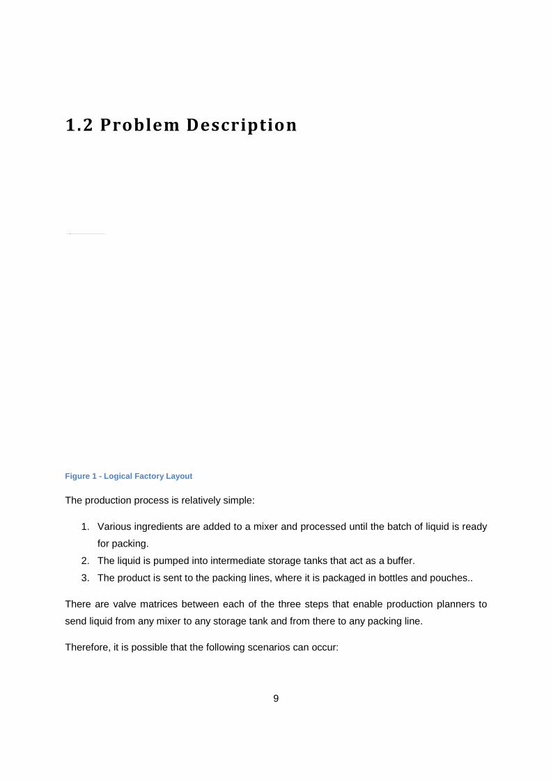
1.2 Problem Description

Figure 1 - Logical Factory Layout

The production process is relatively simple:

1. Various ingredients are added to

for packing.

2. The liquid is pumped into intermediate storage tanks that act as a buffer.

3. The product is sent to the packing lines,

There are valve matrices between each of the three steps that enable production planners to

send liquid from any mixer to any storage tank and from there to any packing line.

Therefore, it is possible that the following scenarios can occur:

9

Description

The production process is relatively simple:

Various ingredients are added to a mixer and processed until the batch of liquid is ready

The liquid is pumped into intermediate storage tanks that act as a buffer.

The product is sent to the packing lines, where it is packaged in bottles and

es between each of the three steps that enable production planners to

send liquid from any mixer to any storage tank and from there to any packing line.

Therefore, it is possible that the following scenarios can occur:

a mixer and processed until the batch of liquid is ready

The liquid is pumped into intermediate storage tanks that act as a buffer.

where it is packaged in bottles and pouches..

es between each of the three steps that enable production planners to

send liquid from any mixer to any storage tank and from there to any packing line.

10

1. One mixer supplies multiple packing lines

2. Many mixers supply one packing line

3. Multiple mixers supply multiple packing lines.

Some products (such as Domestos and Omo Bleach) contain bleach. Bleach cannot be mixed

with other products, and cleanouts after running bleach products need to be extremely

thorough. Therefore it is deemed best by Subject Matter Experts (SMEs) and management that

bleach products are kept entirely separate from the rest of the plant – resulting in two separate

sections that can be scheduled and simulated individually.

1.2.1 Mixers

In some cases, mixers have to receive special modifications to be able to make certain

products. For example, it is possible to produce Fabric Wash and Fabric Conditioner in the

same mixer. However, the mixer needs to be fitted with certain special components that are

necessary in some cases to produce specific products. Therefore, if a mixer is earmarked for

producing Fabric Wash only, it won’t be fitted with the necessary components to produce Fabric

Conditioner too, and it won’t have the capability to make both.

With regards to the different mixer sizes available: various options exist, but since FEED for the

plant is already well underway, it has been decided to use 15 m3 tanks only. The batch-cycle

times of these tanks for each liquid type can be estimated by SMEs but are uncertain.

There should always be a greater amount of each specific liquid made (in tonnes per hour) than

the packing lines require. This calculation should include all machines involved in making a

certain product at each instant. This does not imply, however, that a discrete-time LP is

required. The complexity of multiple machines working with the same liquid can be captured

with a continuous-time LP (Majozi and Zhu, 2001).

Another layer of complexity is that one liquid, such as one of the Sunlight Dishwashing Liquid

variants, can be packaged into several different formats, including different bottle and pouch

sizes. Therefore, if a mixer is supplying multiple packing lines, they may be producing different

products concurrently, all made with the same liquid. This introduces difficulties when defining

product types in the simulation, which will be dealt with later.

11

1.2.2 Packing lines

Products are available in several formats:

1. Bottles

2. Pouches

3. “Sausages” (a type of pouch)

Each format is packed by a packing line that can do only that format.

Various bottle line models can be ordered, including high-speed, medium-speed, and low-speed

versions. The pouch lines, sachet lines, and sausage lines are available in only one speed.

Each packing line is capable of producing multiple sizes of packaging, except the sachet and

sausage lines. However, producing two products with a large difference in size after one

another complicates the change-over process. Therefore, it is deemed best if similar sizes are

made together. Each packing line is capable of packing bottles or pouches at a certain speed

depending on the package size, with larger sizes taking longer to pack.

1.2.3 Changeovers

Once a product has been made, a clean-out must be performed on the affected equipment to

flush residue from the tanks, pipes, and nozzles. The offending chemicals are usually perfumes

or colourants but can also be specific ingredients of the previous product. Also, every time the

bottle type or pouch size at a packing line changes, a changeover must be done to adjust the

equipment to the new bottle size and shape. This changeover (known as a size change-over)

involves installing different spare parts on the packing line and making a few adjustments to the

electronic settings. If only the bottle shape changes, and not the size as well, fewer changes will

be required.

The changeover time required will differ according to the preceding and subsequent product.

This is known in literature as sequence-dependent changeover times.

Product change-overs are sequence-dependant because of several factors:

• in some cases, perfume or colourant A will mask B, but not the other way around

12

• some products, like Domestos, are inherently good at washing away residue of previous

products without suffering in quality

• some products are thicker and more viscous than others and takes longer to wash out

During equipment cleanouts, all pipes and nozzles are thoroughly washed out with hot water

and selected chemicals. Sometimes, a “pigging” approach will also be applied. In this approach,

a special piece of sponge (the “pig”) is forced through the pipe system by water pressure. It

scrubs the pipes from the inside as it moves along. While this is done, the tanks containing the

various raw materials such as perfume and colourants are cleaned out. In this regard, operator

skill (and motivation) comes into play – it’s sometimes possible to let the raw material tanks run

lower than the recommended level in anticipation of an upcoming changeover. When the

changeover commences, the tanks are already nearly empty.

If an equipment cleanout must be done, a size or shape change-over will also be required –

bottle shapes and sizes differ to indicate to the customer that the product contains a different

liquid. Even within the same brand, different bottle colours or label designs are used to make

products easily distinguishable for the consumer. Sometimes, only the bottle size will be

changed while still packing the same liquid. In this case, no clean-out will be required.

In conclusion, tables need to be set up detailing the change-over time from each product to

every other product that is likely to be produced on the same equipment. One table will be

required for each packing line model, and one for the product changeovers to be done in the

mixers and tanks. The values in this table will be determined in consultation with SMEs. There

are two reasons for this:

1. In cases where Unilever has a plant elsewhere in the world using the exact same

equipment (which is by no means the case for most of the machines), local operating

conditions at those sites could skew results;

2. Production managers from that plant will have to be consulted in any case to understand

their operating rules. Their operators may, for example, be forbidden for some reason

from letting raw material levels run low as a pending changeover approaches.

13

The values will only function as a starting point anyway – once the plant is up and running, they

will regularly be updated using Unilever’s thirteen-week average “Demonstrated Capability”

policy, to be discussed in more detail later.

1.2.4 Tanks

Unilever policy dictates a six-hour buffer between making and packing. This will be used to

determine the size of the storage tanks. Since the storage tanks are non-dedicated, determining

how many are needed is a non-trivial problem. However, the non-dedicated design may lead to

fewer tanks being needed. Simulation will be instrumental in this regard. Discrete-event

simulation have been used previously to determine capacity requirements while taking cost and

other factors into account (Zhu, Hen and Teow, 2012) and can readily be applied to determine

the number of tanks needed under a particular schedule.

Another design decision to be made is whether the number of tanks can be doubled while

halving their capacity. This will likely require a slightly higher investment level will also result in a

more flexible storage system. It may even lead to fewer total tanks being required.

1.2.5 Scheduling production for a batch plant with uncertain

process times

To arrive at the amount of time available for production each year, the number of non-productive

days as well as a set time for product innovations is set aside. In the highly competitive FMCG

industry, new products need to be brought to market constantly to keep customers intrigued.

Testing of these products will be done in the product innovations time slot.

Unilever is one of many large companies using the popular enterprse resource management

(ERM) program SAP. One of the many components of this system is one that does sales

forecasting. From the sales forecasts, it draws up required production quantities. However, it

does not specify the optimal sequence in which to produce those products, or the best lot sizes

for each run.

Each week, the planning department will get sales forecasts for the following four weeks from

SAP. They will then try to schedule this by hand to arrive at a workable schedule for the month

ahead.

14

In addition to the amount of products that must be made, a certain amount must be held at the

end of each week. For example, management has determined that, for product A, 2.5 week’s

“cover” is required. This means that the next two-and-a-half weeks’ worth of sales must be kept

in stores as a minimum stock level. The planners will add the next two week’s forecasted sales,

and include half of the third week’s sales. This is the amount of product A that must be in stock

at the end of the week. For simplicity’s sake, weekly sales will be assumed to occur at the end

of each week. Therefore, the amount of product that must be produced in week i can be

calculated as:

Required Production(i) = Required Inventory (i) + Sales (i) – Inventory (i – 1)

Having arrived at the required volumes for each product, it is a challenge to schedule production

on an hour-by-hour basis if process times are uncertain. Therefore, for the purposes of

planning, a fixed processing time will be used. Once a schedule has been created, this plan will

be tested in a DES that takes variable process times into account to see if the schedule works

within the allocated time. The fixed process times are determined using a 13-week rolling

horizon – the “demonstrated capacity” is calculated using a weighted average of the times in

this period. To verify the distributions used in the DES to determine variable times, time studies

will have to be conducted in the new plant once commissioned and up and running.

In the end, production orders are sent to the shop floor in terms of number of units to be

produced before conducting a change-over and switching to the next product. If an interruption

occurs, production will resume until the required number of units have been produced, as

opposed to a fixed time. This is why continuous-time scheduling is superior to discrete-time

scheduling in this application.

More ways of handling uncertain process times will be examined in the literature review.

1.3 Chapter Summary

When several alternatives are encountered during the design process, design decisions will be

supported by building a simulation for each alternative. In some cases, the production schedule

can also be used to pick one alternative over another – if, for example, a valid schedule for a

15

certain configuration cannot be found, and the scheduling system has been validated

previously, we know that we have to change something in the design. Once the plant is up and

running, the combination of the DES and the scheduling system will be invaluable to the plant

managers.

16

Chapter 2

2.1 Introduction

The problem of production scheduling is very well-examined in literature. Not only are

sequencing and scheduling problems challenging, but solving them can have large commercial

value. Ample incentive thus exists to pursue this field of study.

Furthermore, advances in digital technology has made discrete-event simulation commonplace

for many engineering problems.

The two techniques complement each other – a Discrete-Event Simulation (DES) for the new

facility will require some sort of schedule to run on, and the schedules generated by the

scheduling system will need to be tested and rated on a simulation model before being used.

However, the DES and the scheduling system must first be validated individually.

2.2 Literature Review - Simulation

A framework for developing DES models was developed by (Manuj, Mentzer and Bowers,

2009). This framework provides certain standards to modellers with the aim of improving rigor in

simulation – according to the authors, rigorous simulations are reliable simulations. The main

points are given below:

1. Formulate the problem

2. Specify dependent and independent variables

3. Develop and validate conceptual model

4. Collect data

5. Develop and verify a computer-based model

6. Validate the model

7. Perform simulations

17

8. Analyze and document the results

Each step will be examined in detail in the Research Methodology section.

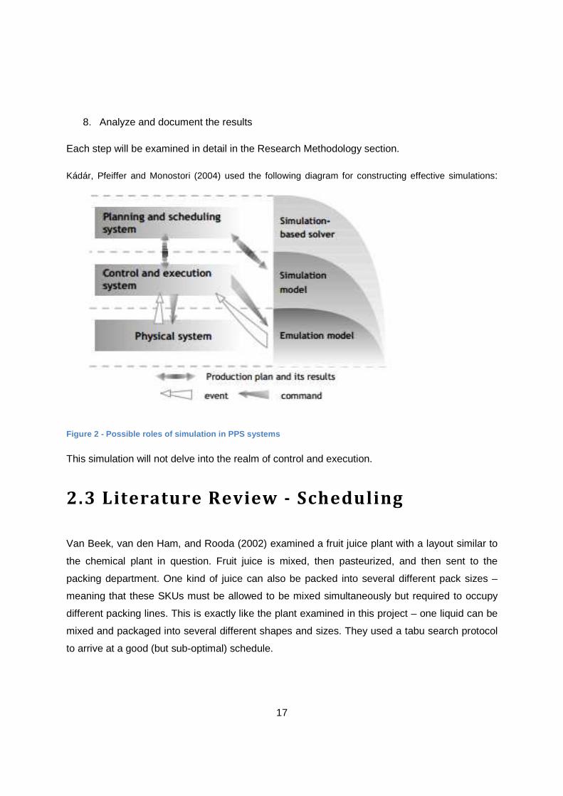
Kádár, Pfeiffer and Monostori (2004) used the following diagram for constructing effective simulations:

Figure 2 - Possible roles of simulation in PPS syst ems

This simulation will not delve into the realm of control and execution.

2.3 Literature Review - Scheduling

Van Beek, van den Ham, and Rooda (2002) examined a fruit juice plant with a layout similar to

the chemical plant in question. Fruit juice is mixed, then pasteurized, and then sent to the

packing department. One kind of juice can also be packed into several different pack sizes –

meaning that these SKUs must be allowed to be mixed simultaneously but required to occupy

different packing lines. This is exactly like the plant examined in this project – one liquid can be

mixed and packaged into several different shapes and sizes. They used a tabu search protocol

to arrive at a good (but sub-optimal) schedule.

18

Batch production scheduling and discrete-event simulation is used either concurrently or

iteratively to some extent to arrive at a plan for maximising the return-on-investment of a factory

in several papers. Examples are (Azzaro-Pantel et al., 1998), (Baudet et al., 1995), (Hung and

Leachman, 1996), and (Moon and Phatak, 2005).

A fundamental problem in batch-process scheduling for a chemical plant is that process times

are uncertain, as was mentioned before.

Hung and Leachman (1996) concluded that the easiest way of production planning is assuming

steady production levels from machines (as used in the initial simulation in this project) but that

this strategy is outdated. The production schedules drawn up by Azzaro-Pantel et al. (1998),

Baudet et al. (1995), and Mockus and Reklaitis (1997) all use fixed process times.

This is in contrast to Sohoni, Lee and Klabjan (2011). This paper investigates ways to generate

flight schedules for airlines with linear programs. The authors use a random variable to

represent flight times but limit this value between a minimum and maximum acceptable time.

This problem is similar to scheduling production runs in that limited resources have to be

scheduled for unknown blocks of time while meeting demand. The paper also presents a

method for determining on-time performance for each flight. This may be useful to ensure than

an intermediate resource (such as a mixer) finishes its run in time for the next resource (like a

packing line) to continue production, but not so early as to have liquid sitting in tanks for

extended periods of time. A major difference between that problem and this one, however, is

that the run lengths can be varied in a chemical plant but we cannot arbitrarily cut the flight

distance between two cities in half.

Where Sohoni, Lee and Klabjan (2011) examined bounded uncertain times in the context of an

airline, Lin, Janak and Floudas (2004) studied this in isolation. They take into account the

variability in processing times, demand, and cost of raw materials.

Azzaro-Pantel et al. (1998) used Genetic Algorithms to determine the order in which batches of

silicon should arrive at a given workstation. The number of batches to be processed was known

beforehand. This strategy requires that the solver software can interface with the DES software

– each sequence the solver generates is tested in the DES and the results are fed back into the

Genetic Algorithm. The difficulty in applying this approach to the problem at hand is the same as

19

with the airline scheduling problem (Sohoni, Lee and Klabjan, 2011). It is also not ideal to

determine run lengths beforehand since this should be determined by the scheduling system.

2.4 Combining DES and Scheduling

Moon and Phatak (2005) used an iterative process between an ERP system (which uses fixed

process times) and a DES program (which allows for uncertain process times, breakdowns and

maintenance) to arrive at a new process time that was then inserted into the ERP system - and

treated as a fixed time for the purpose of scheduling. This is similar to using a Monte Carlo

simulation to arrive at a mean and using that as a fixed duration, but more sophisticated.

If the production scheduling strategy is seen as an interactive process, fixed times can be

justified by using mean processing times and adjusting these regularly. In an interactive

scheduling strategy, the schedule takes inputs from the plant’s actual performance. Therefore,

the planners will re-run the scheduling system after each production run with the observed times

of the previous run as the initial state. The scheduling system will then generate the schedule

for the rest of the time period. If actual times continue to differ from planned times, the planners

may adjust the expected time for the relevant processes for future reference. This will be

implemented in accordance to Unilever’s 13-week rolling-horizon Demonstrated Capacity

calculation.

This strategy is currently the policy at the plant in question – production is scheduled for each

week based on the mean production times demonstrated over the preceding weeks.

2.5 Chapter Summary

The problem of scheduling production is very well-examined in literature. A wide variety of

approaches are used by researchers, from simulating ants and DNA to linear programming.

Discrete-event simulation is a younger discipline due to the high demands it places on computer

equipment, but neverthless, a methodology for developing these models exists and can be

applied to produce reliable simulations.

20

Chapter 3

3.1 Research Methodology

The scheduling system continues with the current management policy of using a rolling horizon

to determine average process times and using this as a fixed duration when planning. In later

versions of this system, variability in processing times and even demand can be taken into

account using the methods developed by Lin, Janak and Floudas (2004).

Data with regards to the following was gathered by consulting SMEs:

• Packing line performance

• Mixer performance

• Product/product compatibility

Other data came from Unilever management:

• List of SKUs

• Demand forecasts

From this, the pre-simulation calculation sheets mentioned previously was drawn up.

The main project phases are shown in the diagram on the next page:

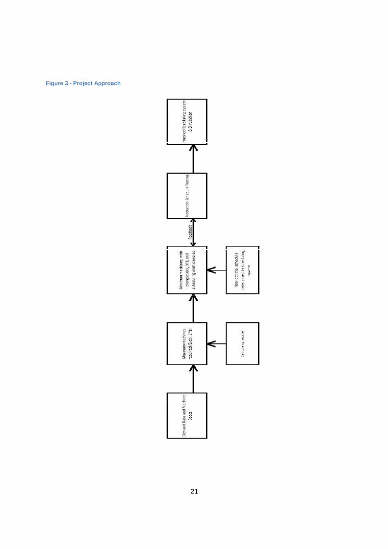
21

Figure 3 - Project Approach

22

3.1.1 Minimum machines required

Initially, demand projections and machine performance specifications were used to determine

the minimum number of machines of each type required. This took into account changeovers,

breakdowns, operational inefficiencies, and scheduling inefficiencies, but did so by applying a

series of simple fractional multipliers to the maximum production capacities of the equipment

involved. (The theoretical maximum production of a machine would be multiplied by 0.7 to get

the desired OEE, and then by another factor to take scheduling inefficiencies and changeovers

into account. The resulting figure would be used as the maximum production.) In this step, linear

programming and a spreadsheet was used concurrently to determine the minimum number of

machines required. This was used as a ballpark figure for the next step of the process.

In the spreadsheet, production was allocated to each packing line and mixer individually. The

spreadsheet checked that produced volumes matched demand. It also checked that

instantaneous demand from the packing lines does not exceed supply from the mixers, and that

each machine stayed within its capacity limit. However, it could not deal with complex situations

where multiple packing lines are being fed by multiple mixers and producing several different

SKUs.

The linear program used the projected demand for each product by year and simply calculated

the minimum number of machines needed to meet that demand. It minimized the number of

machines bought over the period in question.

3.1.2 Discrete-event simulation

To construct a more realistic simulation, discrete-event simulation is required. This has been

done using a sample production schedule which was drawn up manually by the planning

department. Both the model and production schedule was initially made with the number of

machines specified in the previous step in mind. The model and production schedule was then

adjusted as the FEED process progressed.

As mentioned before, the simulation should be able to give statistics about various aspects for

each production schedule used. These include performance indicators like waiting times and

utilisation.

23

Initially, a Monte Carlo simulation was planned, but this concept was abandoned because

insufficient data on machine performance is available, and because it was difficult to capture the

complexities of breakdowns and changeovers without resorting to the heavy-handed strategy of

using a multiplier.

SMDP

The Simulation Model Development Process by Manuj, Mentzer and Bowers (2009) was used

to construct a rigorous DES of the planned factory.

SMDP entails the following:

1. Formulate the problem

The purpose of this simulation is to determine whether the factory will be able to meet

projected demand as it is planned, to determine where equipment levels may be altered

(such as more or fewer tanks), and to test production schedules in terms of validity and

efficiency.

2. Specify dependent and independent variables

Independent variables:

• Batch cycle times

• Number of mixers of each type

• Number of tanks

• Number of packing lines of each type

• Demand projections

• Time available for manufacture each year

• OEE’s for all equipment

• Production Schedule

Dependent variables:

• Capacity utilisation

• Idle time

• WIP levels

24

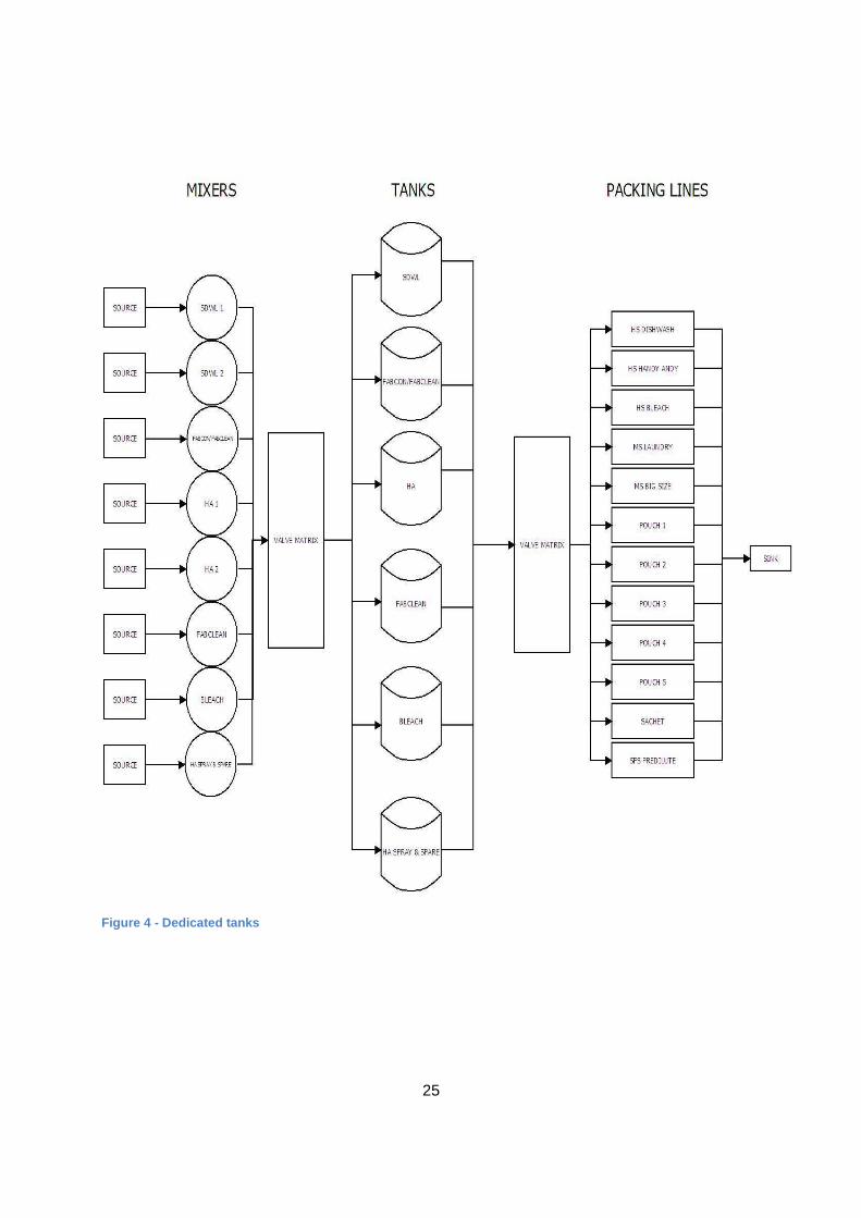
3. Develop and validate conceptual model

Figures 4 and 5 below will serve as a high-level conceptual design of the simulation

itself. There are several ways to approach the problem of simulating this plant and each

diagram is intended to illustrate one such approach.

Each block describes a component that will be placed in the simulation. These

components either represent real-world machines directly (such as the mixers) or are

required by the simulation program itself (such as the source and sink items). Flow items

are created in the source objects and move along the arrows until they reach the sink,

where they will be removed from the simulation.

The plant’s inbound logistics will be to the left of these diagrams – this department will

feed raw materials into the mixers. The source objects are, however, not meant to

simulate the inbound logistics of the factory but simply generate the flow-items that are

necessary for this DES.

The outbound logistics section is to the right of the diagram.

Both the inbound and outbound sections are deemed to be out of scope and it is

assumed that both have infinite capacity to give and receive without delay.

An important output of the simulation modelling is the number of tanks required. There

are two main approaches to design the tanks:

1. Let each product have its own, dedicated tank object.

a. The tank can then be set to have infinite capacity. This will allow the

modellers to see the maximum product levels in the tank with a certain

production schedule.

b. The tank can also be set to a realistic level such as 30 m3. The modellers

can then see whether the tank is a bottleneck at that size or not and try

out various other sizes.

This approach is illustrated on the next page:

25

Figure 4 - Dedicated tanks

26

2. Let several tanks shared amongst the mixers. This is illustrated below:

Figure 5 - Non-dedicated tanks

In this arrangement, liquid is simply sent to the first available tank. The simulation will be

used to determine the minimum number of tanks required to ensure at least one empty

tank will be available when required.

Optimisation of the production schedule will, in many cases, result in some tanks being

used almost exclusively for certain products. The scheduling system will do this to avoid

unnecessary changeovers.This will avoid the need for conducting a change-over for that

tank. Therefore, both approaches have value. Currently, management is leaning towards

the first approach. This is safer and guarantees that each mixer will always have enough

tank space available. If one can conclude from the simulation that some of those tanks

will remain unused for long periods, the non-dedicated approach will be considered.

27

Another important design decision to be made with the simulation is to investigate the

best size of the tanks. We may halve the size of the tanks and double their number, as

mentioned before. We can then investigate this scenario and conclude whether it’s a

financially sound decision or not.

4. Collect Data

The reader is referred to the section called Data Collection.

5. Develop and verify computer-based model

The simulation will be built using Flexsim. Flexsim provides the ability to build discrete-

event simulations (DES’s) and present the results as a 3D model. This makes it easy to

visualise what will be transpiring on the factory floor in specific scenarios. Initially, there

was some difficulty in acquiring a full license for Flexsim. At the time, model-building

could only proceed as small “blocks” of logic on the trial version. These blocks of logic

formed a proof-of-concept that demonstrated that a full, working model could be built

using an enterprise license. Together, they can also be used for validation.

6. Validate Model

The “blocks” of logic mentioned in the previous step include the following concepts:

• Generating the required number of flow items

• Sending these flowitems from machine to machine according to either:

• A pre-defined schedule

• A set of pre-defined rules

• Using a specific processing speed (each machine can process flowitems at

certain rates)

• Conducting change-overs correctly

• Handling batching correctly (mixers produce batches of flow-items at a time while

packing lines process items at a continuous rate)

These proof-of-concept models will be discussed in the Logic Blocks section below.

28

7. Perform Simulations

Once the number of mixers and packing lines were fixed by the Front-End Engineering

Design (FEED), the simulation was run several times with various numbers of tanks to

determine how many would be needed.

8. Analyze results

The real value in having a simulation model will only become apparent when the plant is

up and running and it can be used to manage the plant. However, the mode seemed to

give the best results at a level of twelve tanks, down from the initial sixteen tanks.

Logic Blocks

Initially, a sample-sized Flexsim simulation was built that has the same functions as the full-

scale model. This was done due to difficulty in acquiring a license. It will be apparent that the

different modes can operate together without interfering in each other’s operation. The full-scale

model combines the logic of all these blocks.

Flexsim Background

This is a short overview of Flexsim’s functions. A basic understanding of these will be required

to understand the rest of this section.

The modeller can enter event-based code (in a specialised form of C++) for each of the many

blocks available.

The code in a block’s OnEntry section will execute when a flow item enters the object, for

example. Other events include OnExit, OnReset, sending and receiving messages, and more.

One can therefore inform the simulation by means of C++ what to do in specific cases.

Each machine also has a handy function called Pull Requirements. In this section of the model,

one can specify exactly which flow items must be “pulled” into the machine. Each flow item can

be given various attributes such as an item type, a unique number, a certain colour and shape,

and many more variables. Flowitems can be pulled according to these attributes.

Flexsim also has a feature called Global Tables. These are data tables in which you can track

various numbers. This is used to contain the schedule, processing times, and changeover

29

times. Each machine can look in the global table containing its schedule to see which item to

process, how long to take when conducting a changeover, etc.

One can read and write values to one of the global tables from within the code. Therefore it is

possible to update the tables as production progresses.

Scheduling in Flexsim

As was noted in previous reports, there is some difficulty in the fact that we work with several

classes of liquids that can be further subdivided into variants and pack sizes.

Flexsim has a handy setting that triggers a changeover state in some components if the

itemtype they’re processing differs from the previous type. There are two problems with this:

1. We want a machine to do a changeover as soon as its done with a product (assuming

it’s scheduled to do a different product next). In this configuration, however, the machine

only starts when the next item arrives. This would not be acceptable on the shop floor.

As an example, a packing line may be scheduled to package 5 batches of a product.

The schedule then allows for, say, two hours’ worth of idle time before a different product

will be packed. We’d want the operators to do their one-hour changeover as soon as

they’re done with the first product and then be idle for an hour. This will allow greater

flexibility – if the next product comes early, the line will be ready. It is certainly not

acceptable for the line to start the changeover after having been idle for two hours, and

this is unfortunately not possible with a pre-set on Flexsim.

2. How to differentiate between products containing the same liquid but with different

packaging, such as Regular Sunlight Dishwashing Liquid 750ml & 400ml? These

products should look identical to the mixers because they contain the same liquid. But

the packing lines should not be able to move from one to the other seamlessly. A

changeover is required for them.

The answer is to implement a custom-made batch tracking system. The “Labeller” object seen

in figure 8 applies a label to each passing batch object. Each flow item represents one cubic

metre of fluid. The value is read from a global table. A separate block of code increments the

value in the global table for each flow item created. It would seem more straightforward to apply

30

this label directly, but due to the fact that one cannot send variables directly from one event

handler to another, this workaround is necessary.

Note that we can give each flow item a unique ID and also an itemtype. The itemtype represents

the various liquid types in the factory. The scheduling system keeps track of what product is

represented by each unique item ID.

This solves the change-over problem – the scheduling system will tell us what to produce, and

how much of it. It can then easily output this data in an Excel table and specify between which

numbers changeovers will be required and how long it will take.

Since the schedule now controls the simulation, we can prevent things like incompatible liquids

mixing on that level and do not need to write rules about it into the DES.

31

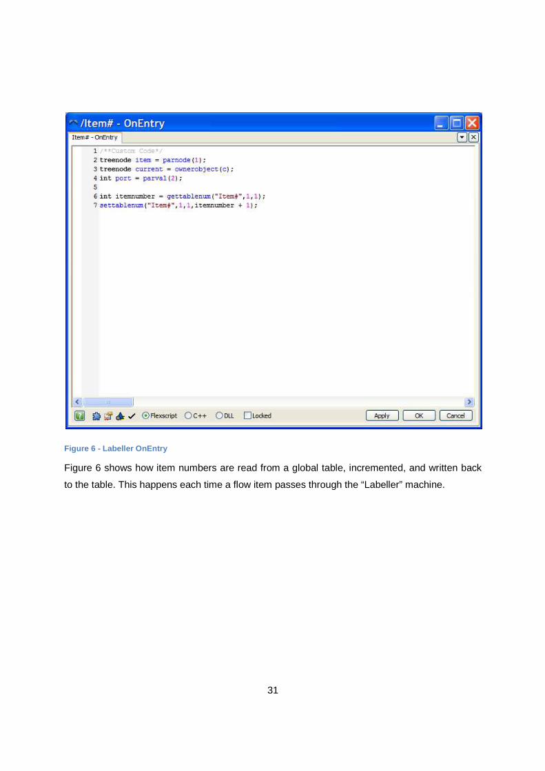
Figure 6 - Labeller OnEntry

Figure 6 shows how item numbers are read from a global table, incremented, and written back

to the table. This happens each time a flow item passes through the “Labeller” machine.

32

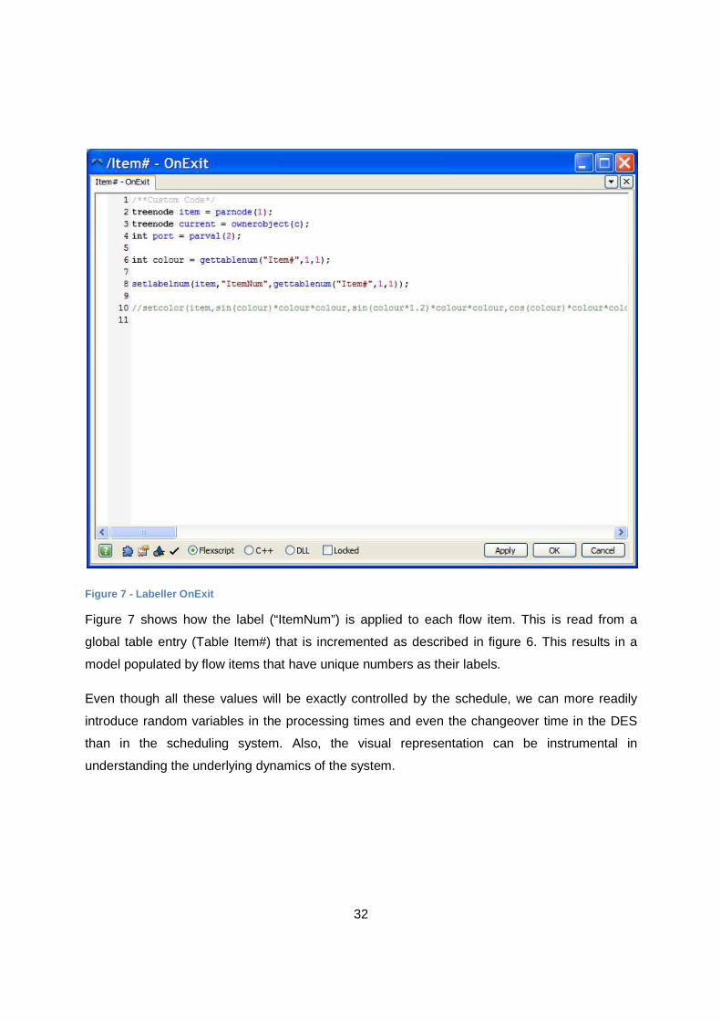
Figure 7 - Labeller OnExit

Figure 7 shows how the label (“ItemNum”) is applied to each flow item. This is read from a

global table entry (Table Item#) that is incremented as described in figure 6. This results in a

model populated by flow items that have unique numbers as their labels.

Even though all these values will be exactly controlled by the schedule, we can more readily

introduce random variables in the processing times and even the changeover time in the DES

than in the scheduling system. Also, the visual representation can be instrumental in

understanding the underlying dynamics of the system.

33

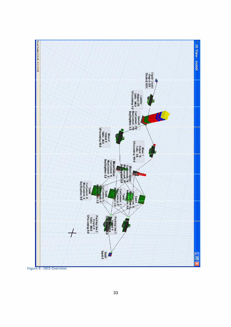
Figure 8 - DES Overview

34

The screenshot in figure 8 shows the entire proof-of-concept model.

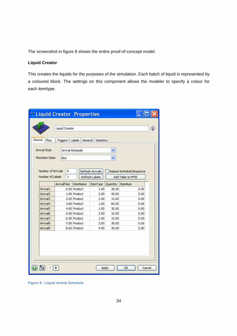
Liquid Creator

This creates the liquids for the purposes of the simulation. Each batch of liquid is represented by

a coloured block. The settings on this component allows the modeler to specify a colour for

each itemtype.

Figure 9 - Liquid Arrival Schedule

35

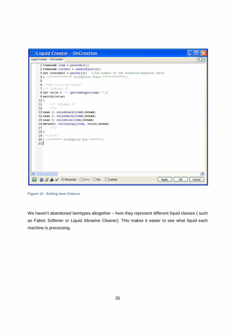
Figure 10 - Setting Item Colours

We haven’t abandoned itemtypes altogether – here they represent different liquid classes ( such

as Fabric Softener or Liquid Abrasive Cleaner). This makes it easier to see what liquid each

machine is processing.

36

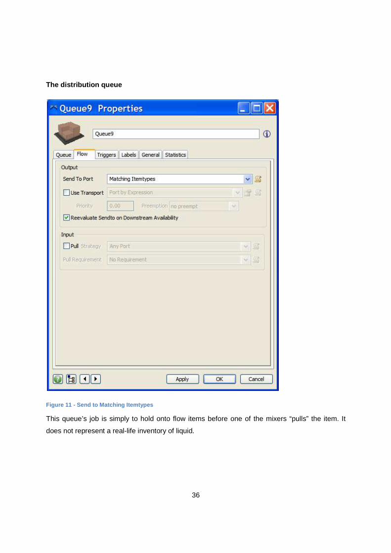
The distribution queue

Figure 11 - Send to Matching Itemtypes

This queue’s job is simply to hold onto flow items before one of the mixers “pulls” the item. It

does not represent a real-life inventory of liquid.

37

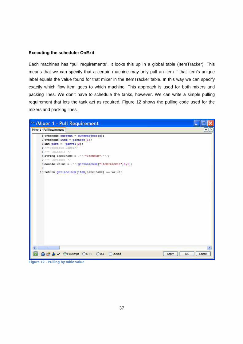
Executing the schedule: OnExit

Each machines has “pull requirements”. It looks this up in a global table (ItemTracker). This

means that we can specify that a certain machine may only pull an item if that item’s unique

label equals the value found for that mixer in the ItemTracker table. In this way we can specify

exactly which flow item goes to which machine. This approach is used for both mixers and

packing lines. We don’t have to schedule the tanks, however. We can write a simple pulling

requirement that lets the tank act as required. Figure 12 shows the pulling code used for the

mixers and packing lines.

Figure 12 - Pulling by table value

38

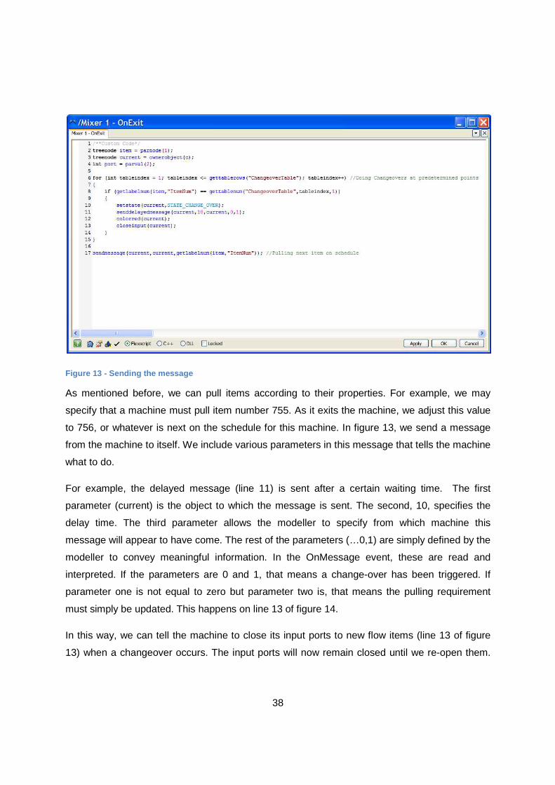
Figure 13 - Sending the message

As mentioned before, we can pull items according to their properties. For example, we may

specify that a machine must pull item number 755. As it exits the machine, we adjust this value

to 756, or whatever is next on the schedule for this machine. In figure 13, we send a message

from the machine to itself. We include various parameters in this message that tells the machine

what to do.

For example, the delayed message (line 11) is sent after a certain waiting time. The first

parameter (current) is the object to which the message is sent. The second, 10, specifies the

delay time. The third parameter allows the modeller to specify from which machine this

message will appear to have come. The rest of the parameters (…0,1) are simply defined by the

modeller to convey meaningful information. In the OnMessage event, these are read and

interpreted. If the parameters are 0 and 1, that means a change-over has been triggered. If

parameter one is not equal to zero but parameter two is, that means the pulling requirement

must simply be updated. This happens on line 13 of figure 14.

In this way, we can tell the machine to close its input ports to new flow items (line 13 of figure

13) when a changeover occurs. The input ports will now remain closed until we re-open them.

39

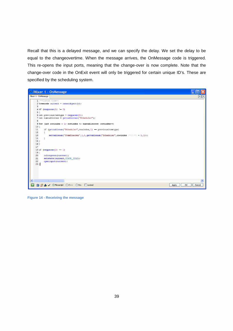
Recall that this is a delayed message, and we can specify the delay. We set the delay to be

equal to the changeovertime. When the message arrives, the OnMessage code is triggered.

This re-opens the input ports, meaning that the change-over is now complete. Note that the

change-over code in the OnExit event will only be triggered for certain unique ID’s. These are

specified by the scheduling system.

Figure 14 - Receiving the message

40

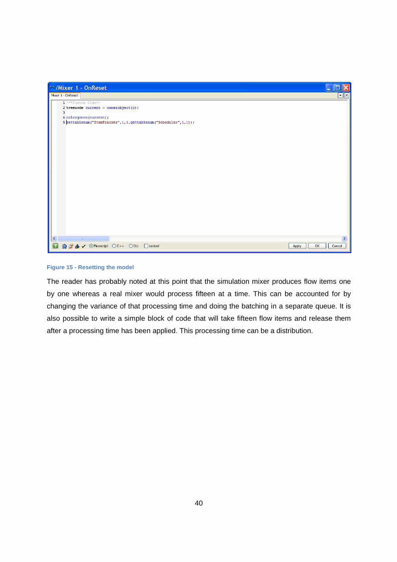
Figure 15 - Resetting the model

The reader has probably noted at this point that the simulation mixer produces flow items one

by one whereas a real mixer would process fifteen at a time. This can be accounted for by

changing the variance of that processing time and doing the batching in a separate queue. It is

also possible to write a simple block of code that will take fifteen flow items and release them

after a processing time has been applied. This processing time can be a distribution.

41

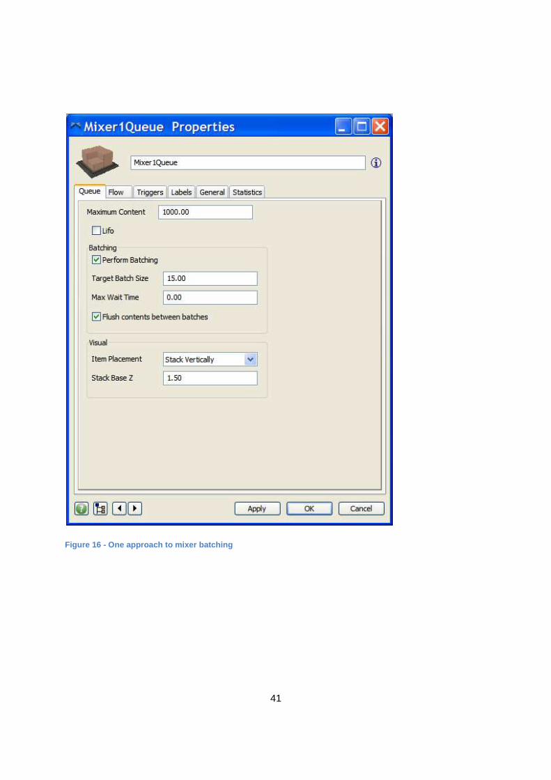
Figure 16 - One approach to mixer batching

42

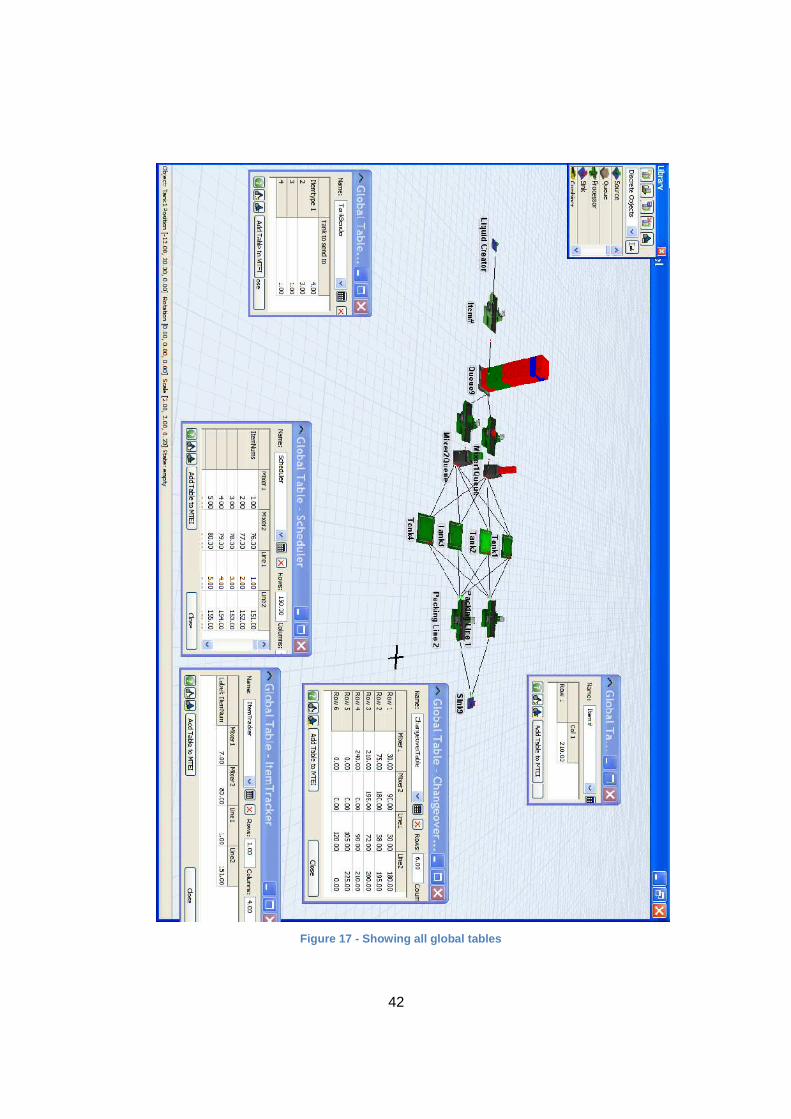
Figure 17 - Showing all global tables

43

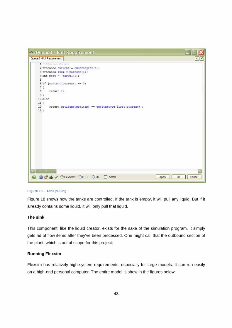
Figure 18 – Tank pulling

Figure 18 shows how the tanks are controlled. If the tank is empty, it will pull any liquid. But if it

already contains some liquid, it will only pull that liquid.

The sink

This component, like the liquid creator, exists for the sake of the simulation program. It simply

gets rid of flow items after they’ve been processed. One might call that the outbound section of

the plant, which is out of scope for this project.

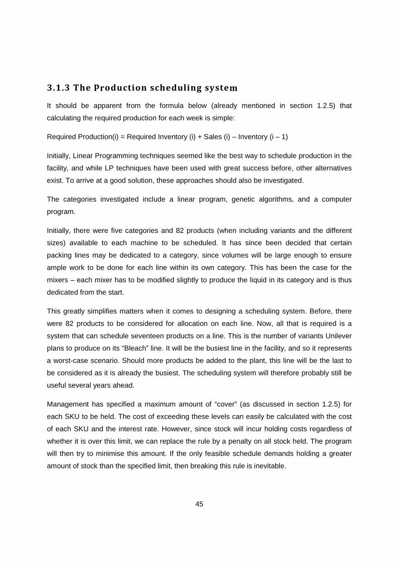
Running Flexsim

Flexsim has relatively high system requirements, especially for large models. It can run easily

on a high-end personal computer. The entire model is show in the figures below:

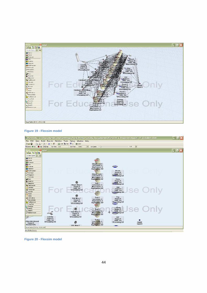
44

Figure 19 - Flexsim model

Figure 20 - Flexsim model

45

3.1.3 The production scheduling system

It should be apparent from the formula below (already mentioned in section 1.2.5) that

calculating the required production for each week is simple:

Required Production(i) = Required Inventory (i) + Sales (i) – Inventory (i – 1)

Initially, Linear Programming techniques seemed like the best way to schedule production in the

facility, and while LP techniques have been used with great success before, other alternatives

exist. To arrive at a good solution, these approaches should also be investigated.

The categories investigated include a linear program, genetic algorithms, and a computer

program.

Initially, there were five categories and 82 products (when including variants and the different

sizes) available to each machine to be scheduled. It has since been decided that certain

packing lines may be dedicated to a category, since volumes will be large enough to ensure

ample work to be done for each line within its own category. This has been the case for the

mixers – each mixer has to be modified slightly to produce the liquid in its category and is thus

dedicated from the start.

This greatly simplifies matters when it comes to designing a scheduling system. Before, there

were 82 products to be considered for allocation on each line. Now, all that is required is a

system that can schedule seventeen products on a line. This is the number of variants Unilever

plans to produce on its “Bleach” line. It will be the busiest line in the facility, and so it represents

a worst-case scenario. Should more products be added to the plant, this line will be the last to

be considered as it is already the busiest. The scheduling system will therefore probably still be

useful several years ahead.

Management has specified a maximum amount of “cover” (as discussed in section 1.2.5) for

each SKU to be held. The cost of exceeding these levels can easily be calculated with the cost

of each SKU and the interest rate. However, since stock will incur holding costs regardless of

whether it is over this limit, we can replace the rule by a penalty on all stock held. The program

will then try to minimise this amount. If the only feasible schedule demands holding a greater

amount of stock than the specified limit, then breaking this rule is inevitable.

46

However, determining the cost of stock-outs is much harder to calculate. One has to account for

not only the cash flow lost with the sale, but also the amount of damage the supplier-client

relationship has suffered. This is very hard to quantify. One must keep in mind that if Unilever’s

supply is unreliable, retailers have to keep more stock as a buffer. This increases prices for the

consumer and decreases profits for both Unilever and the retailer. If retailers refuse to give

Unilever products premium shelf space because it’s no longer profitable for them, Unilever’s

sales and brand strength will suffer. This is unacceptable, so the minimum stock levels are

regarded as absolute rules.

Initially, it was thought that each changeover simply took six hours. We now know this to be

untrue. Change-over times are sequence-dependant, which poses a challenge when

formulating an LP.

In scheduling the new plant, a critical objective is to maximise the utilisation for the packing

lines. The approach required is to schedule the packing lines first, and then the storage tanks

(with the same algorithm), and finally the mixers. When scheduling the storage tanks, their

“production speed” will be the highest flow-rate they can manage. Once we know how fast the

tanks should be supplying liquid, it will be easy to determine the mixers required to create that

fluid.

3.1.3.1 Linear Programming

To limit the number of decision variables, the traditional approach of assigning a decision

variable to each time period should be abandoned since time periods will have to be made

excessively long in order to limit their number. Instead, a continuous-time model can be

implemented. This technique was used by some researchers previously (Majozi and Zhu, 2001),

(Castro, Barbosa-Póvoa and Matos, 2001).

Another approach is the LP used by (Geoffrion and Graves, 1976). This LP resulted in a local

optimum but ran very quickly on a computer from the seventies.

The problem can now be re-stated as a variation of the Travelling Salesman Problem. The

“salesman” represents the settings on each machine. If the salesman is in city A, the machine is

set up to produce product A. To change over to product B, the salesman will have to travel from

47

A to B, and this will take a certain amount of time. When going from B to C, it will take a different

time.

One difference is that the salesman has to spend a certain amount of time at each city. Also,

since stock levels are checked weekly, this means we have to generate four tours, one for each

week. He then has to travel from one loop to another. To illustrate in terms of production lines, a

line may make products A, B, and C in week one. In week two, production of A, C, and D is

required. Note that A and C are made in both week one and week two.

An optimal schedule would probably end week one with either A or C and then start week 2 with

the same product. This will avoid a changeover over the weekend.

One tour would not be able to schedule properly since it would only visit cities (or products) A &

C once, in week one. If A & C are only made once in the four-week period, their run lengths

would have to be quite long. This will result in an unnecessary violation of our maximum stock

levels.

It should also be obvious that the salesman will not have to do a complete a tour of the cities.

The salesperson may start at city A in week one, but will certainly not end week one at A as well

(unless A is the only product for week 1) as this means one unnecessary changeover has been

made back to A. It might not end the month at city A either.

To reconcile these differences, it could prove useful to draw four separate optimal routes

representing one week each. To get the total tour, one could compare each city iA in week A

with each city iB in week B, each of iB with every iC, and each one of that with every iD. Once the

shortest route between all the circles have been found, the paths between iA and iA + 1 , iB and iB

+ 1 , etc. must be eliminated. Therefore, each weekly tour will be broken up and all four joined

together. Since we are dealing with four separate optimal tours being combined, one has to be

wary of local optima. Therefore, all the possible ways of connecting a node in week 1 to the

nodes in weeks 2 – 4 must be evaluated together, or sub-optimality will result. For seventeen

products, this unfortunately results in 174 = 83’521 possibilities after the optimal tours have been

determined. The problem grows exponentially as problem size increases but can be

manageable at this size.

48

To get a near-optimal tour for each week, two methods were considered initially: 2-Opt and Lin-

Kernighan. The 2-opt heuristic tries to exchange two links in the chain. It then makes the

exchange that decreases total travelling time the most, and starts again. It continues in this

manner until no profitable exchanges are possible. A Lin-Kernighan algorithm is like a 2-opt, but

can adjust the number of exchanges dynamically according to problem size and other variables.

However, this system is intended to be used to design the plant as well as run it. In the design

phase, it will be very useful if near-instantaneous results can be had. This will enable designers

to investigate various design scenarios and get immediate feedback about the effect their

decisions will have on the operation of the plant.

Figure 21 - Change-over times

49

Since Lin-Kernighan is unnecessarily complex for a 17-city problem, a 2-opt algorithm was

written. The results of this algorithm were of poor quality and computational time far exceeded

the requirement for near-instantaneous feedback.

Furthermore, we note from figure 19 that the changeover times seems to be grouped into

“neighbourhoods”. Also, in most cases the number of cities in the TSP problem will be far fewer

than 17 – the schedule may call for only some of those products being made. Therefore, a

simple greedy approach was implemented. This resulted in a large decrease in total change-

over time as compared to the sequence set up by the human scheduler. On the sample

schedule, the total change-over time for the bleach line in one month was improved from 97

hours to 55 hours, a 43.2 % decrease.

The exact method of coming to this solution and the entire scheduling program will be discussed

in 3.2.

3.1.3.2 Genetic Algorithms

Another relevant approach is Genetic Algorithms. Enumerating all possible solutions to the

Travelling Salesman Problem for a single week (seventeen products) will result in 17! =

355’687’428’096’000 routes to be evaluated. This is only if all seventeen products are

scheduled. There will also be (17!)/(17-16)! X (1/16!) = 17 instances with only 16 of the

seventeen products, each resulting in 16! = 20’922’789’888’000 routes. If only nine of the

seventeen is chosen, there are (17!)/(17-9)! X (1/9!) = 24’310 instances. Each of those will yield

9! = 362’880 routes. It is therefore quite clear that solving this problem exactly is not practical

with current technology. Genetic Algorithms offer a way of searching through large amounts of

data and arriving at good solutions. It also seems to be a natural fit for the problem at hand. It

will be easy to specify the order of the products, as well as the number of batches required.

However, Genetic Algorithms can have long solving times, and need to be tweaked to get good

results.

3.2 Computer Program

The computer program approach attempts to follow the process human planners use when

scheduling products. It still performs better and faster than human planners because it can

determine the optimum sequence of products instead of relying on a rule of thumb. (Planners

50

have lists giving the preferred order of producing different variants to get a low changeover

time). Also, the trial-and-error involved in scheduling products happen much quicker and are

done more thoroughly.

A definite advantage of this approach is that it can be done in either VBA (which comes with

Excel) or C++ (for which several free IDE’s can be downloaded).

Excel seems like the perfect choice for this task:

• The programmer can achieve a tight integration between the data tables and the VBA

code.

• Data input and output are in a format familiar to all engineers

• This data can easiliy be copied and pasted between applications

One drawback of VBA is that it isn’t the fastest and most efficient language available. However,

the benefits of using a spreadsheet are substantial and outweighs this factor.

A schedule was drawn up by this algorithm with sample data. The same data was used by a

human scheduler. This allows us to compare the two schedules.

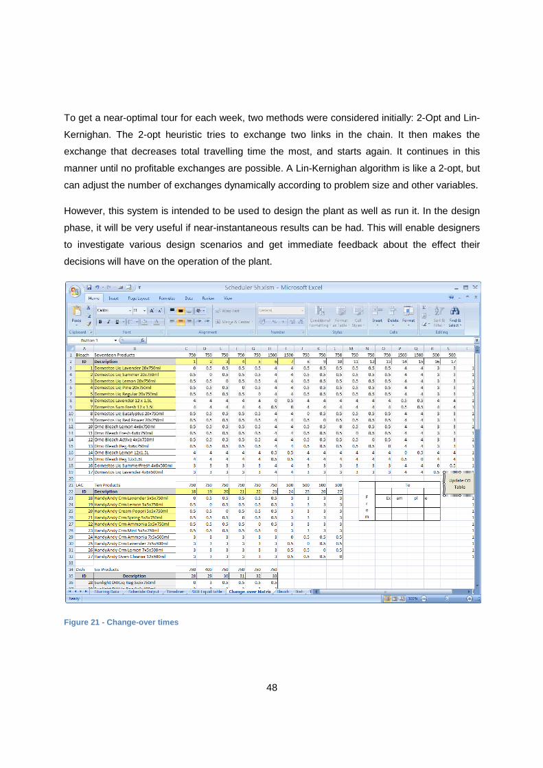
Data entry

The user enters a large number of specifics into the spreadsheet. These include the changeover

times for each line (as seen in figure 19). In this example, the user will then press the button

labelled “Update CO Table”. This is a table is hidden to the user but a screenshot is shown in

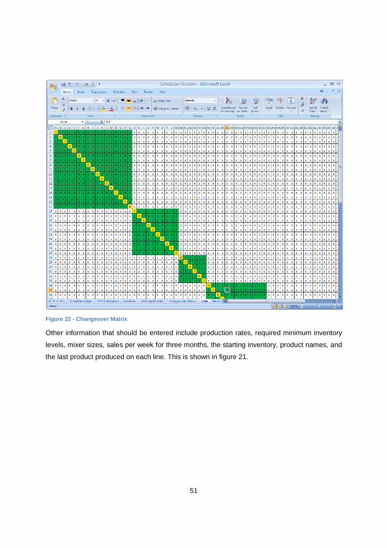
figure 20. The button is linked to VBA code that runs through the values the user entered and

puts them in a matrix format. We can now look at this matrix from elsewhere in the application to

find the changeover time between any two products with the code

Worksheets(“COM”).Cells(Product1, Product2).Value. Another, computationally faster way is to

read these values into a matrix during program execution. Note that if we try two products that

aren’t on the same line, the CO time will be returned as “X”. This lets us know that a changeover

between these products is impossible and irrelevant.

51

Figure 22 - Changeover Matrix

Other information that should be entered include production rates, required minimum inventory

levels, mixer sizes, sales per week for three months, the starting inventory, product names, and

the last product produced on each line. This is shown in figure 21.

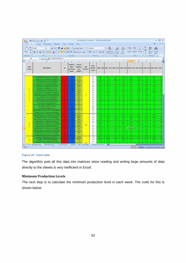
52

Figure 23 - Input data

The algorithm puts all this data into matrices since reading and writing large amounts of data

directly to the sheets is very inefficient in Excel.

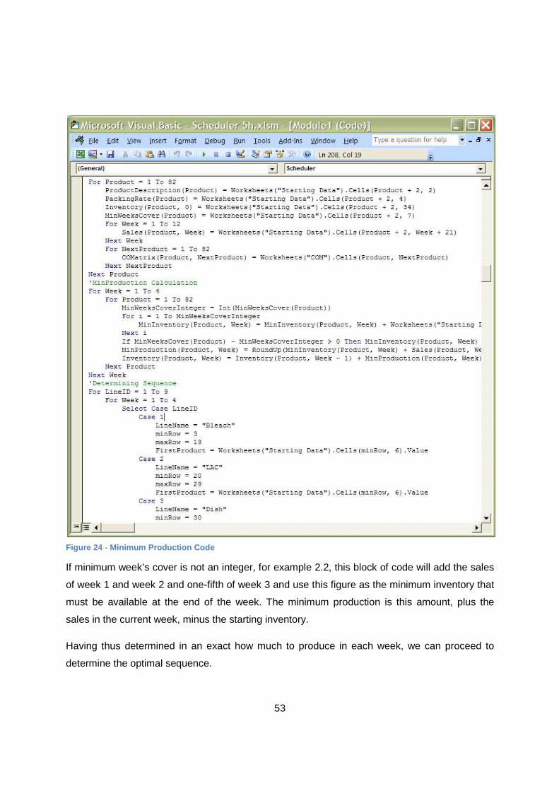
Minimum Production Levels

The next step is to calculate the minimum production level in each week. The code for this is

shown below:

53

Figure 24 - Minimum Production Code

If minimum week’s cover is not an integer, for example 2.2, this block of code will add the sales

of week 1 and week 2 and one-fifth of week 3 and use this figure as the minimum inventory that

must be available at the end of the week. The minimum production is this amount, plus the

sales in the current week, minus the starting inventory.

Having thus determined in an exact how much to produce in each week, we can proceed to

determine the optimal sequence.

54

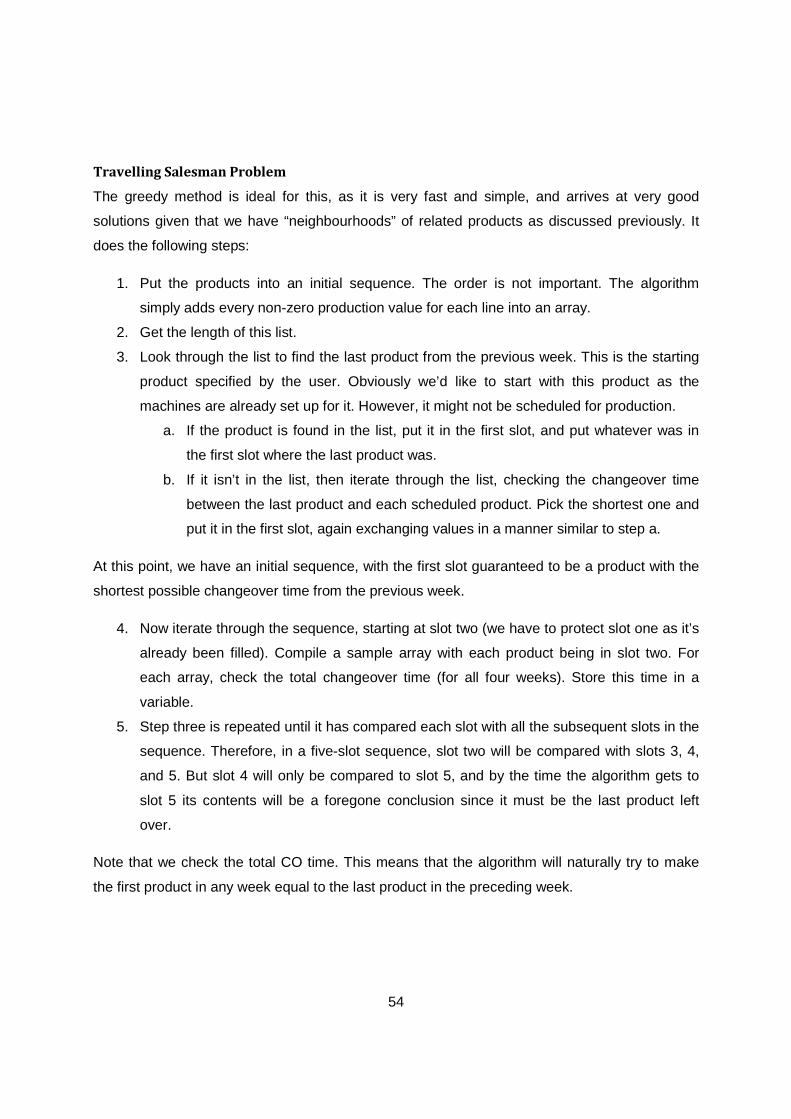
Travelling Salesman Problem

The greedy method is ideal for this, as it is very fast and simple, and arrives at very good

solutions given that we have “neighbourhoods” of related products as discussed previously. It

does the following steps:

1. Put the products into an initial sequence. The order is not important. The algorithm

simply adds every non-zero production value for each line into an array.

2. Get the length of this list.

3. Look through the list to find the last product from the previous week. This is the starting

product specified by the user. Obviously we’d like to start with this product as the

machines are already set up for it. However, it might not be scheduled for production.

a. If the product is found in the list, put it in the first slot, and put whatever was in

the first slot where the last product was.

b. If it isn’t in the list, then iterate through the list, checking the changeover time

between the last product and each scheduled product. Pick the shortest one and

put it in the first slot, again exchanging values in a manner similar to step a.

At this point, we have an initial sequence, with the first slot guaranteed to be a product with the

shortest possible changeover time from the previous week.

4. Now iterate through the sequence, starting at slot two (we have to protect slot one as it’s

already been filled). Compile a sample array with each product being in slot two. For

each array, check the total changeover time (for all four weeks). Store this time in a

variable.

5. Step three is repeated until it has compared each slot with all the subsequent slots in the

sequence. Therefore, in a five-slot sequence, slot two will be compared with slots 3, 4,

and 5. But slot 4 will only be compared to slot 5, and by the time the algorithm gets to

slot 5 its contents will be a foregone conclusion since it must be the last product left

over.

Note that we check the total CO time. This means that the algorithm will naturally try to make

the first product in any week equal to the last product in the preceding week.

55

6. Step three is repeated for each week to ensure we minimise the number of weekend

changeovers to be done.

7. The algorithm gives each week a similar treatment and we end up with a production

sequence.

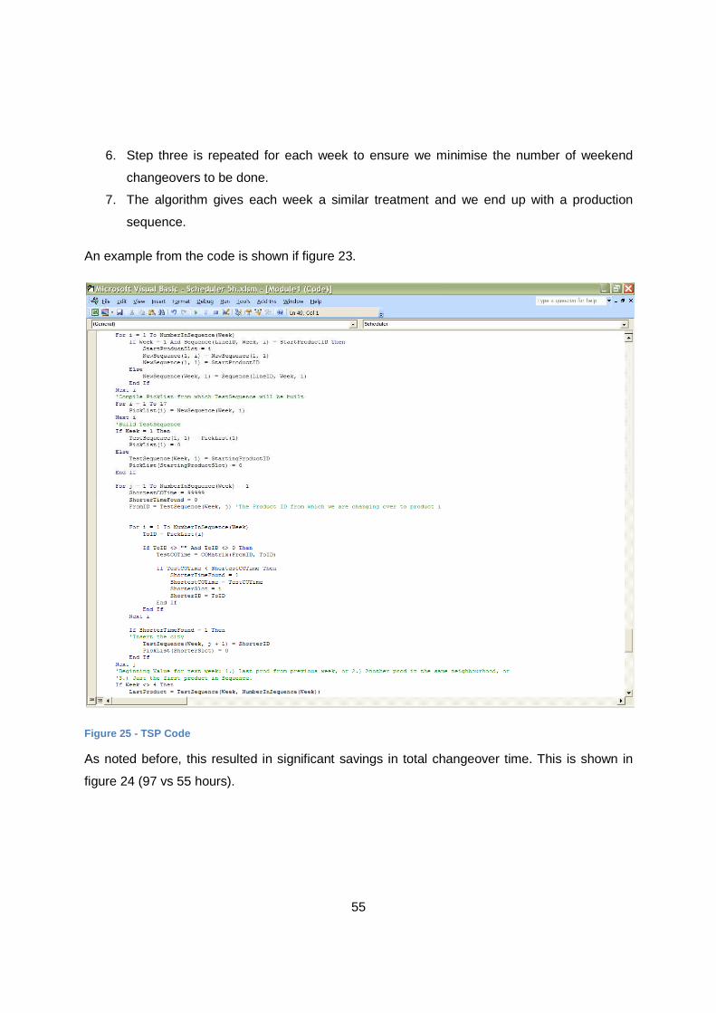
An example from the code is shown if figure 23.

Figure 25 - TSP Code

As noted before, this resulted in significant savings in total changeover time. This is shown in

figure 24 (97 vs 55 hours).

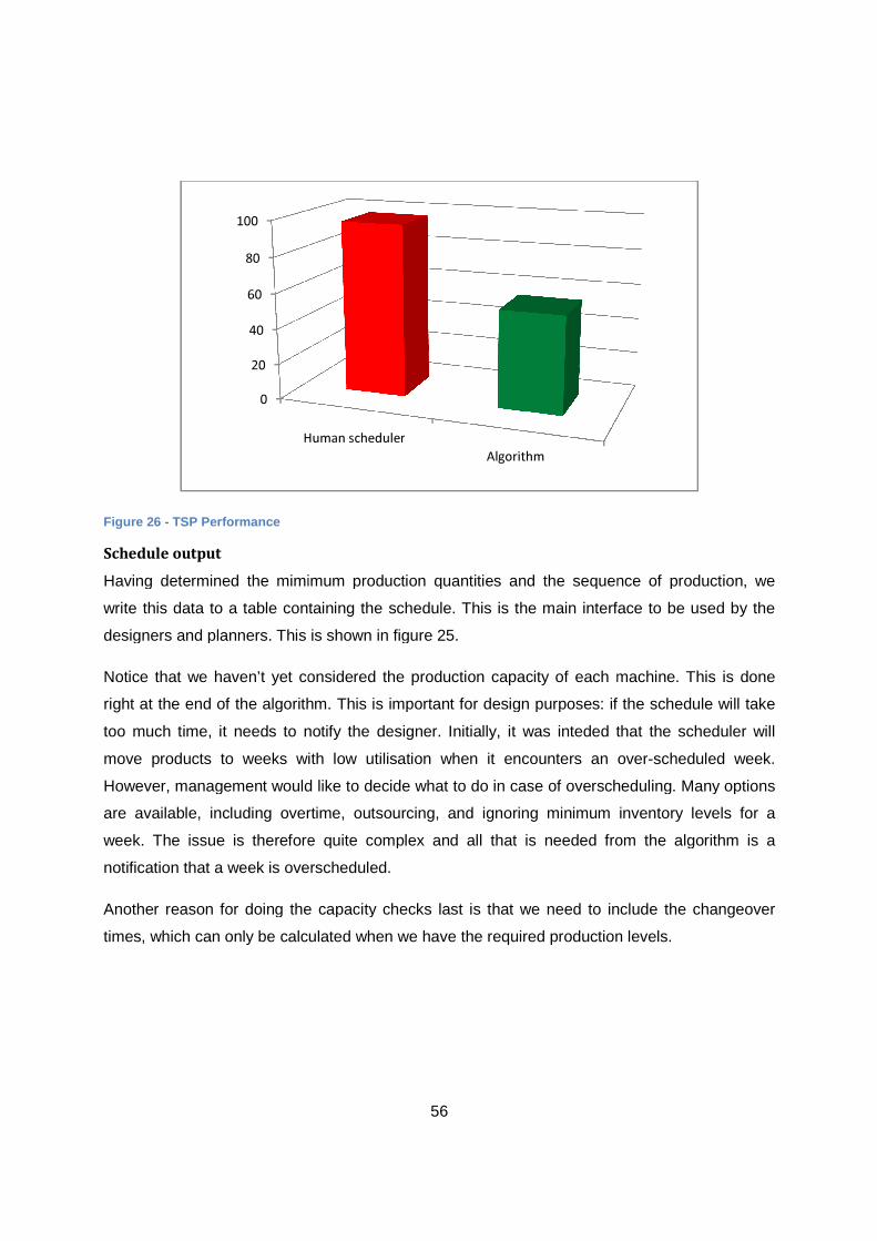
Figure 26 - TSP Performance

Schedule output

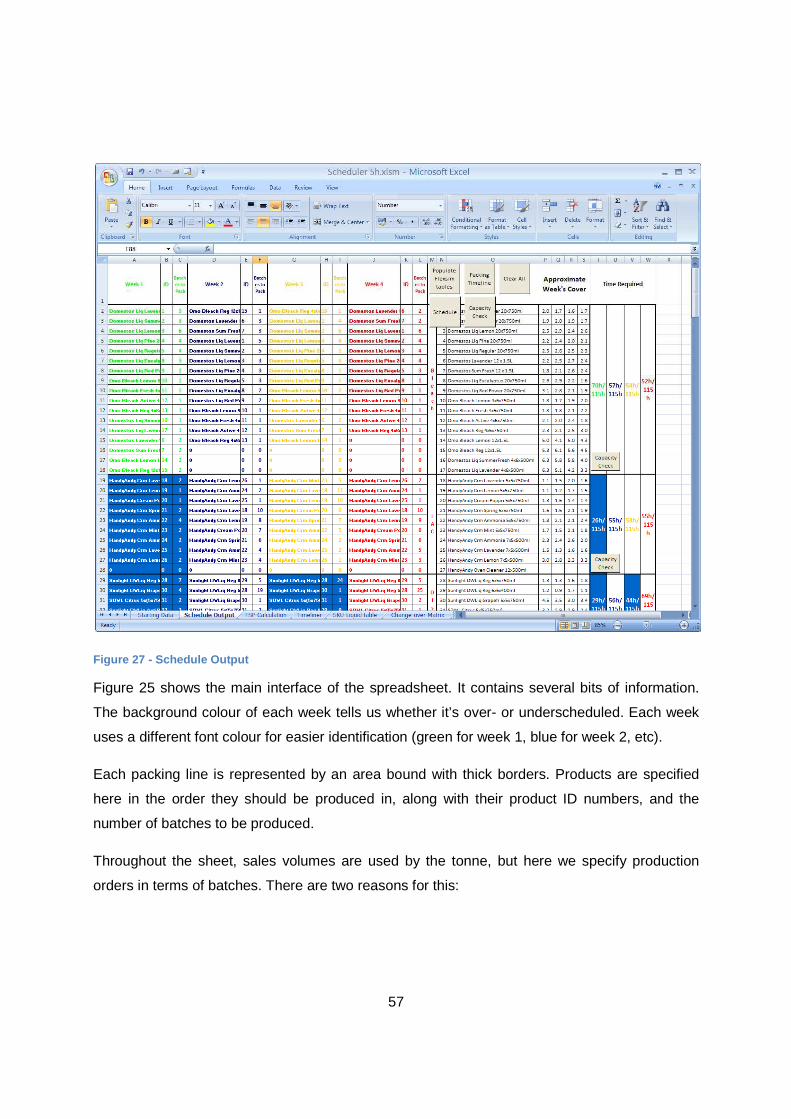
Having determined the mimimum production quantities and the sequence of production, we

write this data to a table containing the schedule. This is the main interface to be used by the

designers and planners. This is shown in figure 25.

Notice that we haven’t yet considered the production capacity of each machine.

right at the end of the algorithm. This is important for design purposes: if the schedule will take

too much time, it needs to notify the designer. Initially, it was in

move products to weeks with low utilisation when it encounters an over

However, management would like to decide what to do in case of overscheduling. Many options

are available, including overtime, outsourcing,

week. The issue is therefore quite complex and all that is needed from the algorithm is a

notification that a week is overscheduled.

Another reason for doing the capacity checks last is that we need to include

times, which can only be calculated when we have the required production levels.

0

20

40

60

80

100

Human scheduler

56

Having determined the mimimum production quantities and the sequence of production, we

write this data to a table containing the schedule. This is the main interface to be used by the

designers and planners. This is shown in figure 25.

ce that we haven’t yet considered the production capacity of each machine.

of the algorithm. This is important for design purposes: if the schedule will take

too much time, it needs to notify the designer. Initially, it was inteded that the scheduler will

move products to weeks with low utilisation when it encounters an over

However, management would like to decide what to do in case of overscheduling. Many options

are available, including overtime, outsourcing, and ignoring minimum inventory levels for a

week. The issue is therefore quite complex and all that is needed from the algorithm is a

notification that a week is overscheduled.

Another reason for doing the capacity checks last is that we need to include

times, which can only be calculated when we have the required production levels.

Human scheduler

Algorithm

Having determined the mimimum production quantities and the sequence of production, we

write this data to a table containing the schedule. This is the main interface to be used by the

ce that we haven’t yet considered the production capacity of each machine. This is done

of the algorithm. This is important for design purposes: if the schedule will take

teded that the scheduler will

move products to weeks with low utilisation when it encounters an over-scheduled week.

However, management would like to decide what to do in case of overscheduling. Many options

and ignoring minimum inventory levels for a

week. The issue is therefore quite complex and all that is needed from the algorithm is a

Another reason for doing the capacity checks last is that we need to include the changeover

times, which can only be calculated when we have the required production levels.

57

Figure 27 - Schedule Output

Figure 25 shows the main interface of the spreadsheet. It contains several bits of information.

The background colour of each week tells us whether it’s over- or underscheduled. Each week

uses a different font colour for easier identification (green for week 1, blue for week 2, etc).

Each packing line is represented by an area bound with thick borders. Products are specified

here in the order they should be produced in, along with their product ID numbers, and the

number of batches to be produced.

Throughout the sheet, sales volumes are used by the tonne, but here we specify production

orders in terms of batches. There are two reasons for this:

58

• We can’t produce a fraction of a batch. Therefore if we want to move production from

one week to another, we have to move an entire batch or nothing at all.

• Production orders are given to the production managers in terms of batches.

Note towards the right of the sheet the heading named “Approximate Week’s Cover”. Under this

heading we calculate the approximate number of week’s sales worth of inventory we’ll have at

the end of each week. The planner will have a range of acceptable values for each of these

values and in future editions of this project, these too can be highlighted according to whether

they’re within target or not.

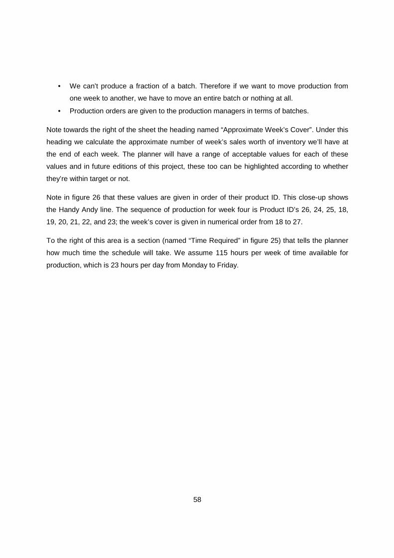
Note in figure 26 that these values are given in order of their product ID. This close-up shows

the Handy Andy line. The sequence of production for week four is Product ID’s 26, 24, 25, 18,

19, 20, 21, 22, and 23; the week’s cover is given in numerical order from 18 to 27.

To the right of this area is a section (named “Time Required” in figure 25) that tells the planner

how much time the schedule will take. We assume 115 hours per week of time available for

production, which is 23 hours per day from Monday to Friday.

59

Figure 28 - Week's Cover

Note in figure 26 the “Capacity Check” button next to each line. This repeats the code from the

main scheduling algorithm that checks if the line can produce the required amount in the time

available. This bit of VBA highlights the weeks according to utilisation level, specifies the

number of hours required for production, and calculates the ending inventory.

60

Figure 29 – Colour-coded weeks

The program highlights the area associated with each week according to it’s utilisation level.

Should it be above the user-specified threshold, the week is highlighted in red. If a week falls

between the specified thresholds (40% and 70% in this case), it isn’t highlighted at all. If the

utilisation is below the 40% specified, the week is made blue. An example is shown in figure 27.

If a week ends up being red, the planner can simply delete some of the values in that week and

enter them in one of the other weeks. Ideally the planner should pick a week that already has

the product being moved in it’s schedule. If that is possible, we can avoid doing another change-

over in that week after moving the batches over. Otherwise, we can simply add it to the bottom

and it will be added to the capacity calculations for that week.

61

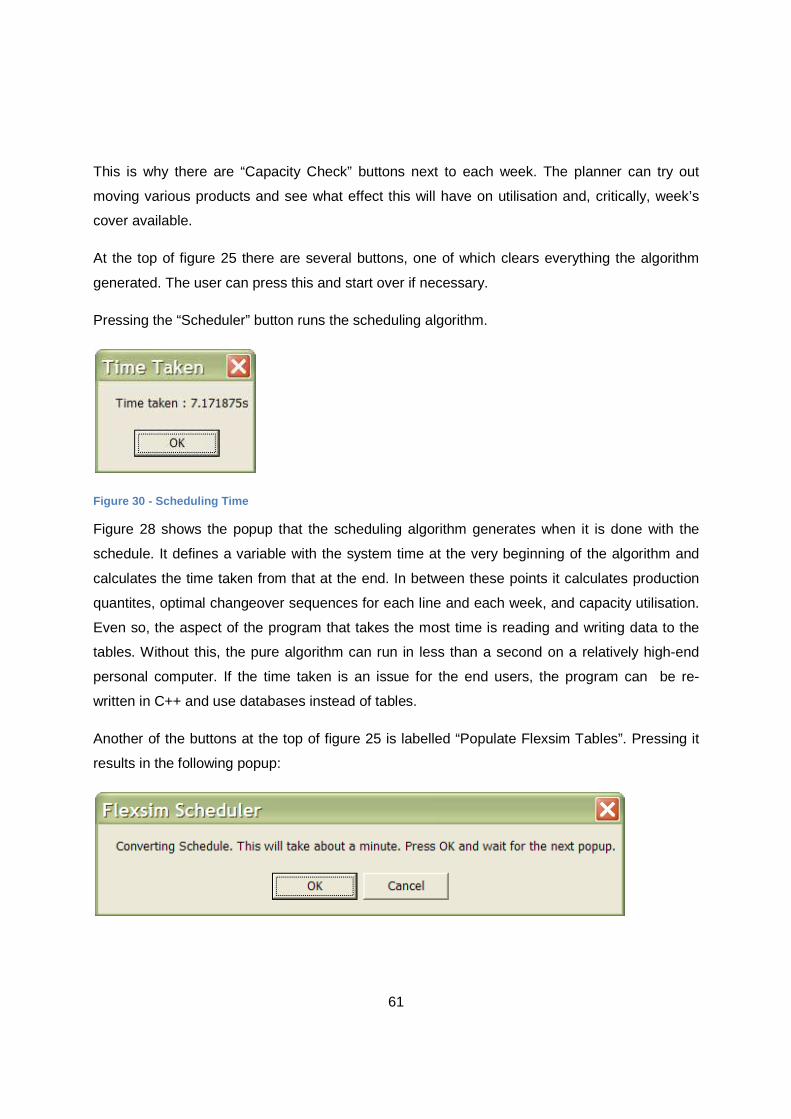
This is why there are “Capacity Check” buttons next to each week. The planner can try out

moving various products and see what effect this will have on utilisation and, critically, week’s

cover available.

At the top of figure 25 there are several buttons, one of which clears everything the algorithm

generated. The user can press this and start over if necessary.

Pressing the “Scheduler” button runs the scheduling algorithm.

Figure 30 - Scheduling Time

Figure 28 shows the popup that the scheduling algorithm generates when it is done with the

schedule. It defines a variable with the system time at the very beginning of the algorithm and

calculates the time taken from that at the end. In between these points it calculates production

quantites, optimal changeover sequences for each line and each week, and capacity utilisation.

Even so, the aspect of the program that takes the most time is reading and writing data to the

tables. Without this, the pure algorithm can run in less than a second on a relatively high-end

personal computer. If the time taken is an issue for the end users, the program can be re-

written in C++ and use databases instead of tables.

Another of the buttons at the top of figure 25 is labelled “Populate Flexsim Tables”. Pressing it

results in the following popup:

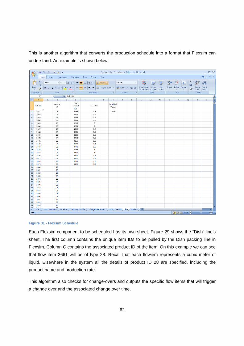
62

This is another algorithm that converts the production schedule into a format that Flexsim can

understand. An example is shown below:

Figure 31 - Flexsim Schedule

Each Flexsim component to be scheduled has its own sheet. Figure 29 shows the “Dish” line’s

sheet. The first column contains the unique item IDs to be pulled by the Dish packing line in

Flexsim. Column C contains the associated product ID of the item. On this example we can see

that flow item 3661 will be of type 28. Recall that each flowiem represents a cubic meter of

liquid. Elsewhere in the system all the details of product ID 28 are specified, including the

product name and production rate.

This algorithm also checks for change-overs and outputs the specific flow items that will trigger

a change over and the associated change over time.

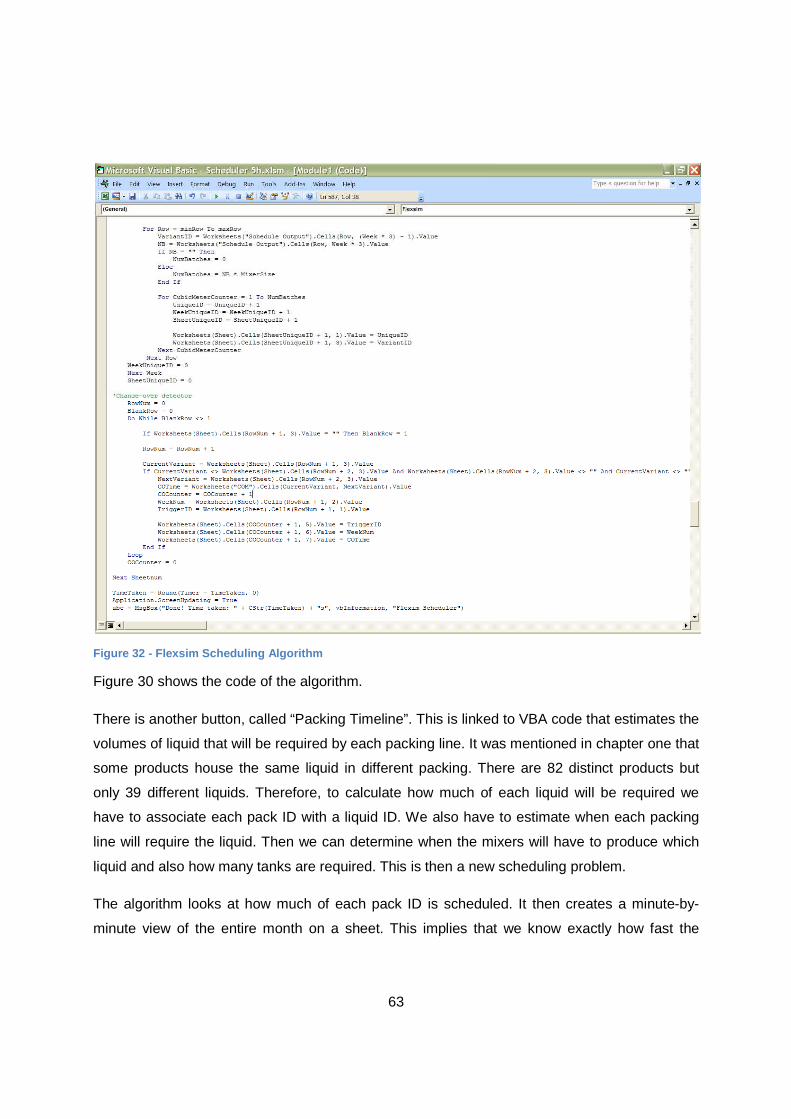
63

Figure 32 - Flexsim Scheduling Algorithm

Figure 30 shows the code of the algorithm.

There is another button, called “Packing Timeline”. This is linked to VBA code that estimates the

volumes of liquid that will be required by each packing line. It was mentioned in chapter one that

some products house the same liquid in different packing. There are 82 distinct products but

only 39 different liquids. Therefore, to calculate how much of each liquid will be required we

have to associate each pack ID with a liquid ID. We also have to estimate when each packing

line will require the liquid. Then we can determine when the mixers will have to produce which

liquid and also how many tanks are required. This is then a new scheduling problem.

The algorithm looks at how much of each pack ID is scheduled. It then creates a minute-by-

minute view of the entire month on a sheet. This implies that we know exactly how fast the

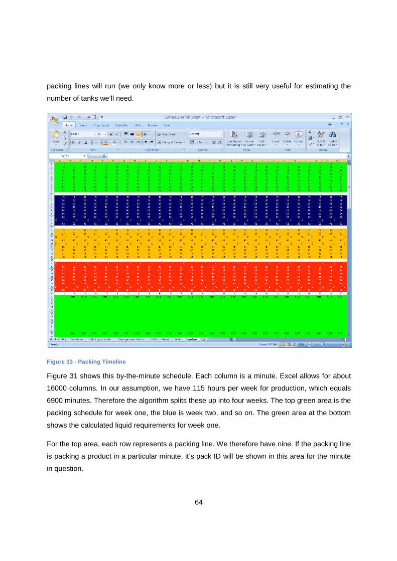
64

packing lines will run (we only know more or less) but it is still very useful for estimating the

number of tanks we’ll need.

Figure 33 - Packing Timeline

Figure 31 shows this by-the-minute schedule. Each column is a minute. Excel allows for about

16000 columns. In our assumption, we have 115 hours per week for production, which equals

6900 minutes. Therefore the algorithm splits these up into four weeks. The top green area is the

packing schedule for week one, the blue is week two, and so on. The green area at the bottom

shows the calculated liquid requirements for week one.

For the top area, each row represents a packing line. We therefore have nine. If the packing line

is packing a product in a particular minute, it’s pack ID will be shown in this area for the minute

in question.

65

The algorithm then iterates through the 6900 values in each week, and checks which liquid will

be required for each product being packed at that minute. It also checks the packing rate in

tonnes per minute. It adds these together and outputs it in the bottom area. Therefore, if we’re

packing Sunlight Dishwash Regular 750ml bottles on the Dish line but also 400ml pouches with

the same liquid on one of the pouch lines, the algorithm will add the liquid requirements (in

tonnes per minute) together and give us that as output.

It should be noted that the change-over time between any two liquids is 30 minutes. This

excludes bleach to non-bleach changeovers which are impossible by design because they take

six hours.

Having these two bits of information, we can determine the maximum number of intermediate

tanks that will be required. We assume that a tank must be available when a liquid is being

packed.

66

Figure 34 - Determining number of tanks

Figure 32 shows the areas specifying the liquid requirements per liquid, per minute. The

selected area is in week four (hence the red highlighting). It shows eight liquids being packed at

that particular moment. The maximum number of liquids being packed simultaneously is nine.

Therefore, if we are packing a maximum of nine different liquids at any one time, we can say

that we need at least nine tanks to contain the nine liquids. Allowing for the fact that a liquid

changeover will make the involved tank unavailable for thirty minutes, we can allow for a safety

factor and add a few more tanks. Extra tanks will also be useful in scheduling the mixers. It’s

allowable for the mixer operators to work overtime and mix the required volumes on the

weekend preceding the packing schedule. However, for this we will require a few tanks to store

the liquid throughout the week until it’s required. Running the schedule on Flexsim seems to

indicate that twelve tanks will be enough for the given volumes.

67

However, the volumes used in the sample schedule are based on sales projected for 2015, and

the factory will hopefully remain in use for long after that. The principle benefit of this method is

then that we now have a tool to determine exactly how many tanks we’ll need for a given table

of sales projections instead of having to rely on rules-of-thumb.

Figure 35 - Scheduling the Mixers

Figure 33 shows the sheet where the deadlines for mixing is calculated. It iterates through the

liquid requirements sheet shown in figure 32. It starts at the end of each week. As it moves

along the columns from minute to minute, it sums the amounts of each liquid required. As soon

as it reaches a multiple of the mixer size for that liquid, it outputs the associated minute number

to this sheet. Therefore we can now know exactly when each mix should be finished. The

algorithm that does this also calculate the size of the gaps between deadlines. If the size

68

between two gaps are smaller than the mixing time, we know we have a clash in the mixer

schedule. The gap lengths are shown in the red area.

The algorithm puts all these deadlines in an array and then sorts it with a form of bubble-sorting,

putting the latest deadlines in front of the earliest ones.

If we then iterate through this array, we will encounter the latest deadlines on Friday afternoon

first and move backwards to Monday morning. Doing it this way, we will assign a mixer to each

deadline. If we find that a deadline occurs close to a previous one, and the required mixer will

be busy at the time, we can simply move that mix bacwards in time. This process is illustrated in

figure 34. In schedule one, we started at the end of the schedule and added mixes as required.

In schedule two, we detected the clash and moved the first mix into the weekend. This is

congruent with the policy that mixers should be able to work overtime to ensure the packing

lines are always fed with sufficient volumes of liquid.

Figure 36 - Mixer schedule clash

69

Currently, the algorithm outputs the deadlines for mixing. In future versions, it will be expanded

to automatically move mixes backwards as required.

3.3 Chapter Summary

Future work

In future, the scheduling system and simulation model can be made to function with tighter

integration. A scheduling system can be written in C++, and it could launch Flexsim with the

correct schedule pre-entered. It could also offer a higher degree of automation, for example

automatcally shifting the mixing schedules when clashes are detected.

Results achieved

We have arrived at an estimate for how many machines are required to meet a certain set of

projected sales figures. More importantly, we now have a system that can be used to verify the

final design for any set of sales figures. Since the project is nearing the end of the design phase,

this will be an invaluable tool.

This system can also be applied when managing the plant once it’s up and running. Various

production strategies can be tested on the simulation. Different schedules can be evaluated for

expected performance.

Should expansions and upgrades be planned, they can easily be tested with the same system.

The system could estimate the increase in operating efficiency to be expected from any

changes. This will be essential when presenting the business case for these changes.

With some effort, this system can also be adapted to other, similar construction projects.

The production scheduling system will be invaluable in operating the new plant at maximum

profitability – the algorithm produced schedules with lower total inventory and lower changeover

times than an experienced human planner from Unilever.

70

Bibliography

Azzaro-Pantel, C., Bernal-Haro, L., Baudet, P., Domenech, S. and Pibouleau, L. (1998) 'A two-

stage methodology for short-term batch plant scheduling: discrete-event simulation and genetic

algorithm', Computers and Chemical Engineering, vol. 22, no. 10, pp. 1461-1481.

Baudet, P., Azzaro-Pantel, C., Domenech, S. and Pibouleau, L. (1995) 'A discrete-event

simulation approach for scheduling batch processes', Computers & Chemical Engineering, vol.

19 Supplement, pp. p633-638.

Castro, A., Barbosa-Póvoa, A.P.F.D. and Matos, H. (2001) 'An Improved RTN Continuous-Time

Formulation for the Short-term Scheduling of Multipurpose Batch Plants', Industrial and

Engineering Chemistry Research, p. 2059–2068.

Figielska, E. (1999) 'Preemptive scheduling with changeovers: using column generation

technique and genetic algorithm', Computers & Industrial Engineering 37 (1999) 81-84.

Geoffrion, A.M. and Graves, G.W. (1976) 'Scheduling Parallel Production Lines with

Changeover Costs: Practical Application of a Quadratic Assignment/LP Approach', Operations

Research, Vol. 24, No. 4 (Jul. - Aug., 1976), pp. 595-610.

Hung, Y.-F. and Leachman, R. (1996) 'A Production Planning Methodology for Semiconductor

Manufacturing Based on Iterative Simulation and Linear Programming Calculation', IEEE

Transactions on Semiconductor Manufacturing, vol. 9, no. 2, May, pp. 257-269.

Kádár, B., Pfeiffer, A. and Monostori, L. (2004) 'Discrete event simulation for supporting

production planning and scheduling decisions in digital factories'.

Lin, X., Janak, S.L. and Floudas, C.A. (2004) 'A new robust optimization approach for

scheduling under uncertainty: Bounded uncertainty', Computers and Chemical Engineering ,

vol. 28, p. 1069–1085.

Majozi, T. and Zhu, X.X. (2001) 'A Novel Continuous-Time MILP Formulation for Multipurpose

Batch Plants. 1. Short-Term Scheduling', Industrial and Engineering Chemistry Research,

November, p. 5935–5949.

71

Manuj, I., Mentzer, J.T. and Bowers, M.R. (2009) 'Improving the rigor of discrete-event

simulation in logistics and supply chain research', International Journal of Physical Distribution &

Logistics Management, vol. 39, no. 3, pp. 172-201.

Méndez, C., Cerdá, J., Grossmann, I., Harjunkoski, I. and Fahl, M. (2006) 'State-of-the-art

review of optimization methods for short-termscheduling of batch processes', Computers and

Chemical Engineering, vol. 30, no. 6-7, May, pp. 913-946.

Mockus, L. and Reklaitis, G.V. (1997) 'Mathematical programming formulatio for scheduling of

batch operations base on nonuniform time discretization', Computers and Chemical

Engineering, vol. 21, no. 10, pp. 1147-1156.

Moon, Y. and Phatak, D. (2005) 'Enhancing ERP system’s functionality with discrete event

simulation', Industrial Management & Data Systems, vol. 105, no. 9, pp. 1206 - 1224.

Rubin, P.A. and Ragatz, G.L. (1995) 'Scheduling in a sequence dependant setup environment

with genetic search', Computers Ops Res. VoL 22, No. l, pp. 85-99, 1995.

Sohoni, M., Lee, Y. and Klabjan, D. (2011) 'Robust Airline Scheduling under Block Time

Uncertainty', Transportation Science, vol. 45, no. 4, pp. 451-464.

van Beek, D.A., van den Ham, A. and Rooda, J.E. (2002) 'Modelling and control of process

industry batch production systems', 15th Triennial World Congress, Barcelona, Spain.

Vin, J. and Ierapetritou, M. (2000) 'A New Approach for Efficient Rescheduling of Multiproduct

Batch Plants', Industrial and Engineering Chemistry Research, vol. 39, no. 11, September, pp.

4228-4238.

Wang, K., Liihl, T., Stobbe, M. and Engell, S. (2000) 'A genetic algorithm for online-scheduling

of a multiproduct polymer batch plant ', Computers and Chemical Engineering 24 (2000) 393-

400.

Young Hoon Lee, A. and Pinedo, M. (1997) 'Scheduling jobs on parallel machines with

sequence-dependent setup times', European Journal of Operational Research 100 (1997) 464-

474.

72

Zhu, Z., Hen, B.H. and Teow, K.L. (2012) 'Estimating ICU bed capacity using discrete event

simulation', International Journal of Health Care Quality Assurance, vol. 25, no. 2, pp. 134-144.