A Direct Method for Trajectory Optimization ofRigid Bodies Through Contact ∗

Michael Posa, Cecilia Cantu, and Russ TedrakeComputer Science and Artificial Intelligence Lab

Massachusetts Institute of TechnologyCambridge, MA 02139

{mposa, ceci91, russt}@mit.edu

September 4, 2013

Abstract

Direct methods for trajectory optimization are widely used for planning locallyoptimal trajectories of robotic systems. Many critical tasks, such as locomotionand manipulation, often involve impacting the ground or objects in the environ-ment. Most state-of-the-art techniques treat the discontinuous dynamics that resultfrom impacts as discrete modes and restrict the search for a complete path to aspecified sequence through these modes. Here we present a novel method fortrajectory planning of rigid body systems that contact their environment throughinelastic impacts and Coulomb friction. This method eliminates the requirementfor a priori mode ordering. Motivated by the formulation of multi-contact dy-namics as a Linear Complementarity Problem (LCP) for forward simulation, theproposed algorithm poses the optimization problem as a Mathematical Programwith Complementarity Constraints (MPCC). We leverage Sequential QuadraticProgramming (SQP) to naturally resolve contact constraint forces while simul-taneously optimizing a trajectory that satisfies the complementarity constraints.The method scales well to high dimensional systems with large numbers of possi-ble modes. We demonstrate the approach on four increasingly complex systems:rotating a pinned object with a finger, simple grasping and manipulation, planarwalking with the Spring Flamingo robot, and high speed bipedal running on theFastRunner platform.

1 IntroductionTrajectory optimization is a powerful framework for planning locally optimal tra-jectories for linear or nonlinear dynamical systems. Given a control dynamicalsystem, x = f (x,u), trajectory optimization aims to design a finite-time input tra-jectory, u(t),∀t ∈ [0,T ], which minimizes some cost function over the resulting

∗A preliminary version of this paper was presented at the 2012 Workshop on the Algorithmic Foundationsof Robotics (WAFR) conference [27]

1

input and state trajectories. There are a number of popular methods for transcrib-ing the trajectory optimization problem into a finitely parameterized nonlinear op-timization problem (see [7]). Broadly speaking, these transcriptions fall into twocategories: the shooting methods and the direct methods. In shooting methods,such as Differential Dynamic Programming (DDP) [20], the nonlinear optimiza-tion searches over (a finite parameterization of) u(t), using a forward simulationfrom x(0) to evaluate the cost of every candidate input trajectory. In direct meth-ods, the nonlinear optimization simultaneously searches over parameterizations ofu(t) and x(t); here no simulation is required and instead the dynamics are imposedas a set of optimization constraints, typically evaluated at a selection of colloca-tion points [19]. Mixtures of shooting and direct methods are also possible, andfall under the umbrella of multiple shooting.

There are advantages and disadvantages to both direct and shooting methods,which are outlined here. For a more detailed comparison, see the survey article[6]. For many problems, direct methods enjoy a considerable numerical advantageover the shooting methods, which can be plagued by poorly conditioned gradients;for instance, a small change in the control input at t = 0 will often have a dramati-cally larger effect on the cost than a small change near time T . Direct methods canalso be initialized with a guess for the state trajectory, x(t), which may be easier todetermine than an initial u(t). A reasonable initial trajectory is generally helpfulin avoiding problems with local minima. Since x(t) is also parameterized, directmethods generate larger optimization problems but this increase in size is partiallyoffset by the sparsity of the resulting problem, allowing efficient (locally optimal)solutions with large-scale sparse solvers such as SNOPT [18], and trivial paral-lel/distributed evaluation of the cost and constraints. Dimitrov et al. demonstratethe numerical benefits of sparse, direct optimization for MPC in [13]. We alsonote that throughout the optimization process, shooting methods that determinethe state trajectory through simulation will always result in dynamically feasibletrajectories. However, in the case of direct methods, solvers enforce the systemdynamics through nonlinear constraints and must first converge to feasibility.

In this paper, we take advantage of the benefits of direct methods and considerthe problem of trajectory optimization for rigid-body systems subject to elastic col-lisions and friction. This is an essential problem for robotics which arises in anytasks involving locomotion or manipulation. The collision events that correspondwith making or breaking contact, however, greatly complicate the trajectory opti-mization problem as they result in large or impulsive forces and rapid changes invelocity. While it is possible to resolve contact through the use of continuous reac-tion forces like simulated springs and dampers, the resulting differential equationsare typically stiff and require an extremely small time step, increasing the size andcomplexity of the problem [7]. For numerical efficiency, a preferred method is toapproximate collisions as impulsive events that cause discontinuous jumps in ve-locity. A popular method for control of such systems is as a autonomous hybriddynamical system that undergoes discontinuous switching (see [39]). The discretetransitions are fully autonomous as we can directly control neither the switchingtimes nor the switching surface.

There are a number of impressive success stories for trajectory optimizationin these hybrid models, for instance the optimization of a 3D running gait [30].These results primarily use direct methods. But they are plagued with one ma-jor short-coming - the optimization is constrained to operate within an a priorispecification of the ordering of hybrid modes. For a human running where motion

2

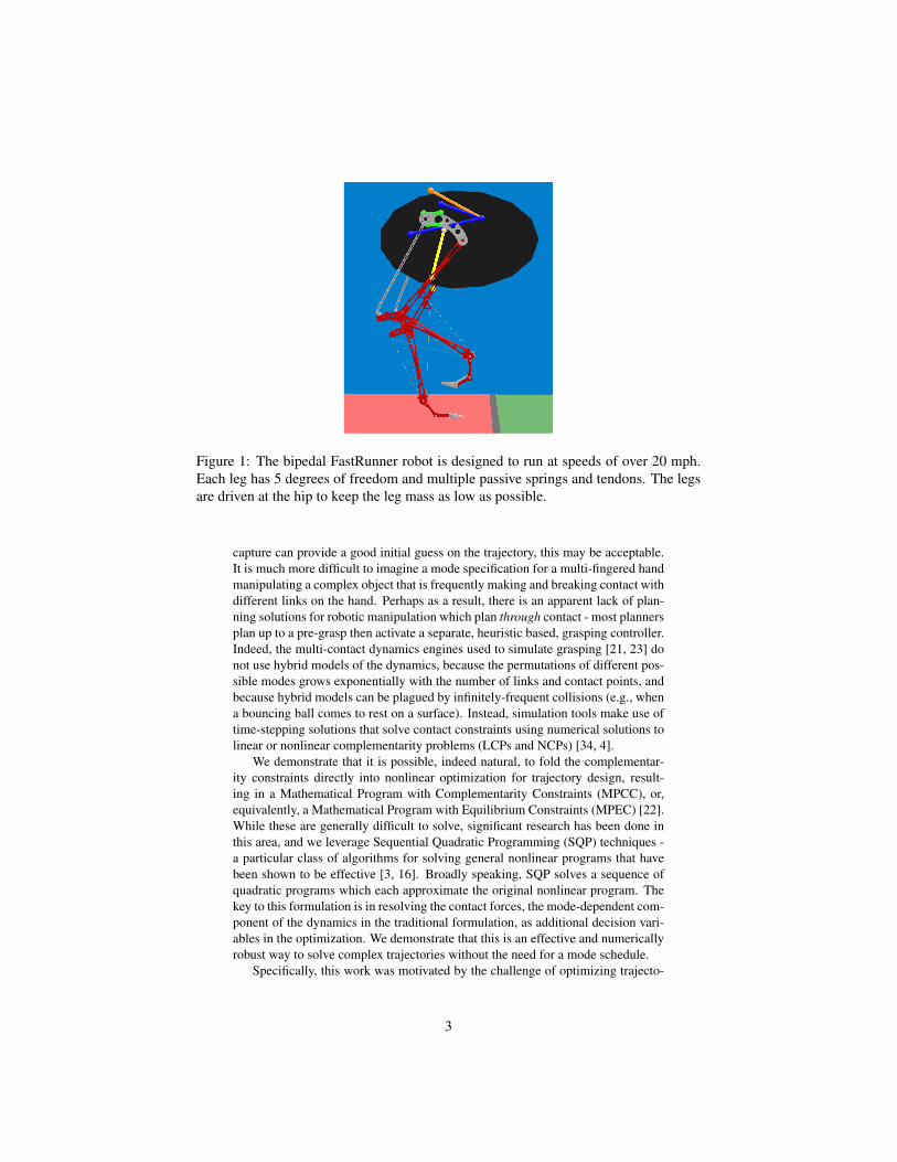
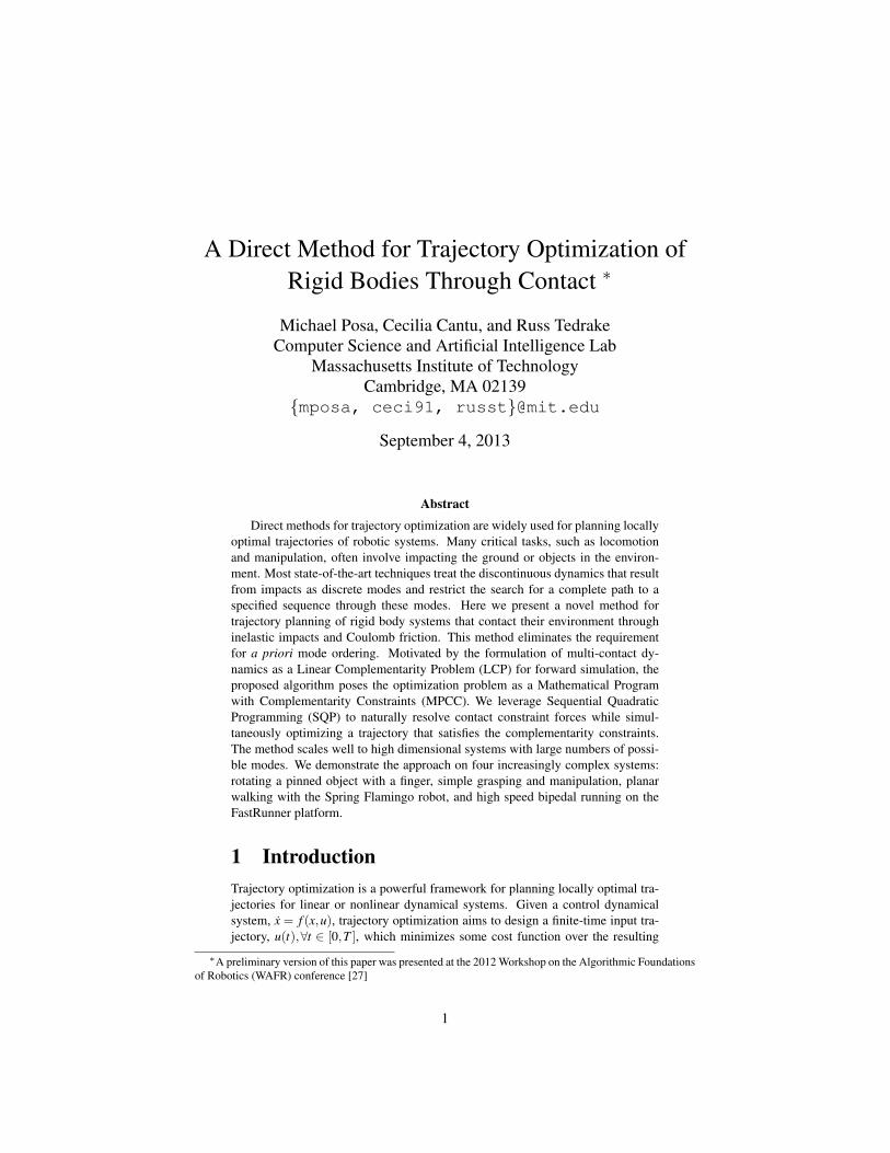
Figure 1: The bipedal FastRunner robot is designed to run at speeds of over 20 mph.Each leg has 5 degrees of freedom and multiple passive springs and tendons. The legsare driven at the hip to keep the leg mass as low as possible.

capture can provide a good initial guess on the trajectory, this may be acceptable.It is much more difficult to imagine a mode specification for a multi-fingered handmanipulating a complex object that is frequently making and breaking contact withdifferent links on the hand. Perhaps as a result, there is an apparent lack of plan-ning solutions for robotic manipulation which plan through contact - most plannersplan up to a pre-grasp then activate a separate, heuristic based, grasping controller.Indeed, the multi-contact dynamics engines used to simulate grasping [21, 23] donot use hybrid models of the dynamics, because the permutations of different pos-sible modes grows exponentially with the number of links and contact points, andbecause hybrid models can be plagued by infinitely-frequent collisions (e.g., whena bouncing ball comes to rest on a surface). Instead, simulation tools make use oftime-stepping solutions that solve contact constraints using numerical solutions tolinear or nonlinear complementarity problems (LCPs and NCPs) [34, 4].

We demonstrate that it is possible, indeed natural, to fold the complementar-ity constraints directly into nonlinear optimization for trajectory design, result-ing in a Mathematical Program with Complementarity Constraints (MPCC), or,equivalently, a Mathematical Program with Equilibrium Constraints (MPEC) [22].While these are generally difficult to solve, significant research has been done inthis area, and we leverage Sequential Quadratic Programming (SQP) techniques -a particular class of algorithms for solving general nonlinear programs that havebeen shown to be effective [3, 16]. Broadly speaking, SQP solves a sequence ofquadratic programs which each approximate the original nonlinear program. Thekey to this formulation is in resolving the contact forces, the mode-dependent com-ponent of the dynamics in the traditional formulation, as additional decision vari-ables in the optimization. We demonstrate that this is an effective and numericallyrobust way to solve complex trajectories without the need for a mode schedule.

Specifically, this work was motivated by the challenge of optimizing trajecto-

3

(a)

(b)

Figure 2: (a) Hybrid trajectories can be found by individually optimizing over the con-tinuous dynamics of a specified mode sequence. Here, the system evolves continuouslythrough one mode before striking a guard. The dashed line indicates the discontinuousjump from one mode to another before continuous evolution in the other mode begins.(b) When the hybrid transition map is more complex, the switching surfaces formedby multiple guards functions may lie close together and the set of possible mode se-quences can be extremely large. In these cases, it is no longer trivial to specify theoptimal mode sequence.

ries for a new running robot called “FastRunner” [12]. FastRunner, illustrated inFigure 1 is a bipedal robot concept designed to run at speeds over 20 mph and up to50 mph. Most notably, FastRunner has a clever, but also complex, leg design withfour-bar linkages, springs, clutches, hard joint stops, tendons and flexible toes. Theplanar FastRunner the model has 13 degrees of freedom, 6 contact points, 16 ad-ditional constraint forces, and only 2 actuators, and was beyond the scope of ourpreviously existing trajectory optimization tools.

2 Background2.1 The pitfalls of mode schedulesFor simple hybrid systems, including point foot models of walking robots, trajec-tories of the hybrid system can be described by smooth dynamics up until a guardcondition is met (e.g., the robot’s foot hits the ground), then a discontinuous jumpin state-space, corresponding here to an instantaneous loss of velocity as energy isdissipated through an impulsive collision–followed by another smooth dynamicalsystem, as cartooned in Figure 2(a). The discrete state, or mode, corresponds to theset of active contacts. The vector field, x = f (x,u), will also be mode dependentdue to continuous forces exerted by sustained contact.

For a fixed mode schedule, direct methods for hybrid trajectory optimizationproceed by optimizing each segment independently, with additional constraintsensuring that the segments connect to each other through the hybrid events.

4

However, when the dynamics are more complex, the geometric constraints im-posed by the hybrid system become more daunting. The FastRunner model has ahybrid event every time that any of the ground contact points (on either foot) makeor break contact with the ground. But the model also undergoes a hybrid transitionevery time that any one of the joints hits a joint-limit, and every time that any oneof the ground reaction forces enters or leaves the friction cone (transitioning froma sticking to a sliding contact). Indeed, the number of possible hybrid modes ofthe system grows exponentially with the number of constraints. The geometry ofthe hybrid guards becomes very complex, as cartooned in Figure 2(b). In thesemodels, small changes to the control input can result in a very different sched-ule of hybrid modes. Restricting the trajectory optimization search to the initialmode schedule can result in a very limited search and in failure to find a feasibletrajectory that satisfies all of the constraints.

Despite the obvious limitation of requiring this mode schedule, it has provensurprisingly difficult to remove this assumption in the direct methods. Slight vari-ations from the original sequence are possible if the formulation allows the timeduration of individual modes to vanish, as in the work of Srinivasan and Ruina[32]. For problems with fewer possible modes, Wampler and Popovic used outeroptimization loops to determine the hybrid mode schedule [38]. In some cases,the combinatorial problem of solving for a mode schedule has been addressed bycombinatorial planners; a variant of the Rapidly-Exploring Random Tree (RRT)algorithm was used in [31] to produce bounding trajectories for a quadruped overterrain. Methods for optimal control which approximate the global optimum, suchas brute force methods based on dynamic programming, have also been applied[9], but are so far limited to low dimensional problems.

2.2 Contact Dynamics as a Complementarity ProblemIn order to avoid the combinatorial explosion of hybrid models, simulation tech-niques in computer graphics and in grasping research use a different formulationof contact, summarized briefly here [37]. In this work, we will focus on systemscomprised of multiple rigid bodies undergoing inelastic collisions and subject toCoulomb friction. Note that in some cases, like FastRunner, the rigid links com-posing the robot will be connected via (massless) passive elements like springs ortendons, though this does not fundamentally change the structure of the equationsof motion. For simplicity, we first discuss the forward dynamics of a rigid-body(e.g., with a floating base) subject to frictionless contact constraints, which can bewritten as the problem of finding the acceleration and contact force vectors:

find q,λ (1)

subject to H(q)q+C(q, q)+G(q) = B(q)u+ J(q)Tλ , (2)

φ(q)≥ 0 (3)

λ ≥ 0 (4)

φ(q)Tλ = 0. (5)

where q ∈ Rn is the vector of generalized coordinates, H(·) is the inertial matrix,C(·, ·) represents the Coriolis terms, G(·) the gravitational forces, and B(·) is theinput mapping. Vector inequalities are to be interpreted as element-wise inequality

5

constraints. For m potential contacts, φ(q) : Rn → Rm where φ(q) ≥ 0 is an in-equality representing a non-penetration constraint. Strict equality φi(q) = 0 holdsif and only if the ith contact is active. λ ∈ Rm represents the constraint forcesacting along the surface normal, and J(·) represents the Jacobian projecting con-straint forces into the generalized coordinates. In simple examples, such as contactbetween a point and a fixed surface, we will take φ(q) to be the signed distancebetween the point and surface and then we have J(q) = ∂φ(q)

∂q . Taken together,(3)-(5) form a complementarity constraint and ensure that the contact forces canbe non-zero if and only if the bodies are in contact. It should be noted that (3) maybe difficult to pose properly in the case where the non-penetrating configurationspace is non-convex, although work has been done in this area regarding simu-lation [26]. Standard variations on this formulation can be made to also addressfrictional contact [37, 8].

The solutions to these dynamics are potentially complex, involving large im-pact forces occurring over very short time periods (e.g., at the moment of a newcollision). In the limiting case of purely rigid bodies, the constraint forces, λ (t),are often modeled with Dirac δ functions, as impulsive events, or through mea-sure differential inclusions [8, 33, 2]. However, many of these complexities can beavoided by discretizing the system in time. Stewart and Trinkle introduced a time-stepping method that only considers the integral of contact forces over a periodand so does not differentiate between continuous and impulsive forces [34].

For the Stewart and Trinkle time-stepping method, the dynamics and constraintterms can be evaluated at the known q, q, allowing an Euler-approximation of thestate at the next time step to be written as the solution to a linear set of equa-tions subject to linear complementarity constraints, resulting in an LCP. 3D con-tact models also fit into the LCP framework, although Coulomb friction cone mustbe approximated by a series of linear constraints. It has been proven that solu-tions exist to this LCP and, under reasonable conditions, that these solutions canbe computed using pivoting methods like Lemke’s Algorithm or more general con-vex optimization algorithms [34, 4, 23]. Here, solving each LCP corresponds tosimulating a single time step. This approach has proved to be remarkably efficientand can rapidly simulate systems with thousands of simultaneous contacts.

2.3 Related WorkA number of researchers are currently pursuing mode invariant trajectory optimiza-tion, as contrasted with the traditional hybrid systems based approach. In [5], Be-rard et al. used the LCP formulation of contact to design trajectories of single bodyon a vibrating plate. Here, they optimize over a small set of parameters describingthe oscillating behavior of the plate and the approach can best be described as ashooting method. Tassa and Todorov have also explored the use of stochastic com-plementarity for optimal control using DDP [36]. As this and similar approachesmake local, gradient-based, improvements to a nominal trajectory, they will notnaturally discover new contact sequences not already present and so rely on thenatural dynamics of the system to make contact. Mordatch et al. demonstratedcontact invariant optimization of complex, lifelike behaviors of humanoid figuresusing relaxations of the contact complementarity constraints in [25]. To pose asimpler problem, Mordatch et al. assume that the limbs of the figures are massless;an assumption we do not make in the current paper. The work of Erez and Todorov

6

optimized a human running gait by smoothing the contact dynamics to make use ofa custom inverse dynamics formulation [14]. In [24], Mordatch et al. include thecontact forces as optimization parameters, similar to the work in this paper and ourpreliminary version [27]. Mordatch includes the feasibility of the contact forces asa penalty term in the optimization cost function, rather than as a direct constraint.Broadly speaking, compared to this paper, the work in [14, 25, 24] make varyingrelaxations of physical or dynamic constraints to pose more tractable (and uncon-strained) optimization problems. Relaxing the constraints allows contact forcesto act at a distance; while this may produce dynamically infeasible trajectories,it has a smoothing effect and provides gradient information that would otherwisebe unavailable in typical shooting methods. Additionally, all three works makeheavy use of inverse dynamics. For highly underactuated systems, like the planarFastRunner robot, arbitrary state or end effector trajectories are not dynamicallyfeasible and inverse dynamics is generally less useful. Formal comparison of thesevarious methods is difficult, as the field has not yet agreed upon a set of canonical,hard problems; this is an important goal for collaborative future

3 ApproachContact constraints formulated using the complementarity conditions fit naturallyinto the direct formulation of trajectory optimization. Rather than solving the LCPfor the contact forces λ at each step, we directly optimize over the space of feasi-ble states, control inputs, constraint forces, and trajectory durations. Treating thecontact forces as optimization parameters is similar to how direct methods treat thestate evolution implicitly. The number of parameters and constraints increases, butthe problem is often better conditioned and more tractable to state of the art solvers.Where g(·, ·) and g f (·) are the integrated and final cost functions respectively, theoptimization problem can be written as

minimize{h,x0,...,xN ,u1,...,uN ,λ1,...,λN}

g f (xN)+hN

∑k=1

g(xk−1,uk), (6)

though any nonlinear objective based on h,x0, ...,xN ,u1, ...,uN ,λ1, ...,λN is alsoallowed.

3.1 Optimization ConstraintsThis optimization problem is subject to constraints imposed by the manipulatordynamics and by rigid body contacts. To integrate the dynamics, both forwardsand backwards Euler methods are equally applicable. Time-stepping simulationmethods commonly use semi-implicit methods, but the dynamics constraints inour optimization problem are already fully implicit and so we chose backwardsintegration for added numerical stability. For ease of notation, we will write Hk =H(qk) and likewise for other matrix functions in the manipulator equations. Whereh is the length of the time-steps and for k = 1, . . . ,N− 1, the dynamics from (2)imply the constraints:

qk−qk+1 +hqk+1 = 0 (7)

Hk+1(qk+1− qk)+h(

Ck+1 +Gk+1−Bk+1uk+1− JTk+1λk+1

)= 0.

7

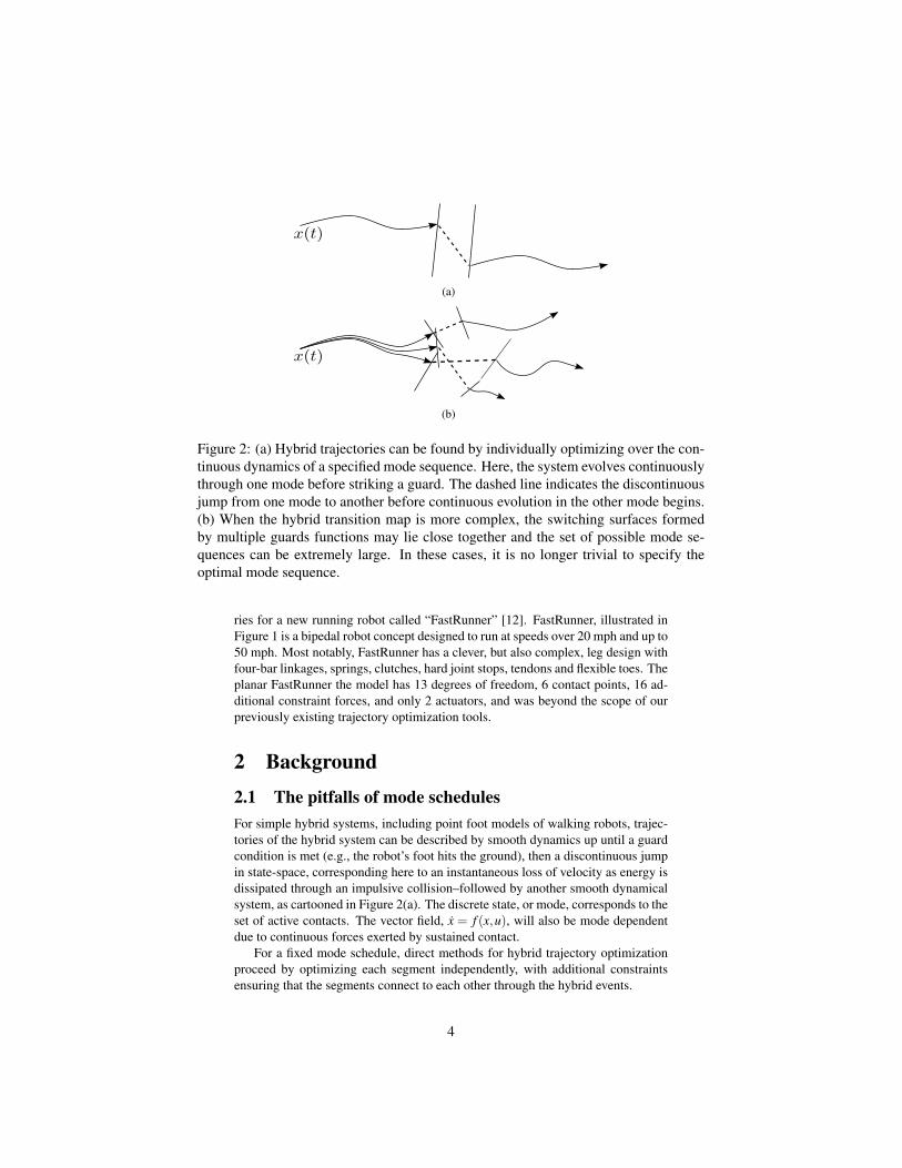
For notational simplicity, we first consider the case where the (frictional) con-tact dynamics are planar and later discuss the extension to 3D contacts. For agiven contact point, write the contact force, λ =

[λ+

x −λ−x λz]T expressed in a

reference frame with x tangent to the contact surface and z normal to the surface.Following the formulation of [34], we have split the tangential force into its posi-tive and negative components and introduce the additional slack variable γ , whichis generally equal to the magnitude of the relative tangential velocity at a contact.We then have the same set of unilateral and bilateral contact constraints:

φ(qk)≥ 0 (8)

λk,z,λ+k,x,λ

−k,x,γk ≥ 0 (9)

µλk,z−λ+k,x−λ

−k,x ≥ 0 (10)

γk +ψ(qk, qk)≥ 0 (11)

γk−ψ(qk, qk)≥ 0 (12)

φ(qk)T

λk,z = 0 (13)(µλk,z−λ

+k,x−λ

−k,x

)Tγk = 0 (14)

(γk +ψ(qk, qk))T

λ+k,x = 0 (15)

(γk−ψ(qk, qk))T

λ−k,x = 0. (16)

where ψ(q, q) is the relative tangential velocity at a contact. Taken together, (8)-(16) are a set of complementarity equations that describe inelastic impacts and aCoulomb coefficient of friction µ . In addition to preventing contact forces at adistance, these complementarity constraints enforce the friction cone and ensurethat, if the contact is sliding, the tangential force properly lies on the edge of thecone and directly opposes the direction of motion. Together, these directly equateto the to the case structure of Coulomb friction where

ψ(qk, qk) 6=0⇒ λk,x =−sgn(ψ(qk, qk))µλz,k

ψ(qk, qk) =0⇒ λk,x ≤ µλz,k.

In addition to expressing frictional contacts, we can also describe simple po-sition constraints such as hard joint limits or kinematic loops in a similar manner.Here, λ is an internal torque or force acting directly on a joint. For example, ifthere is a physical stop enforcing the requirement that q≤ qmax, write

φ(qk) = qmax−qk ≥ 0 (17)

−λk ≥ 0 (18)

φ(qk)T

λk = 0. (19)

It is important to note the relative indexing of the complementarity and dynam-ical constraints. Over the interval [tk, tk+1], the contact impulse can be non-zero ifand only if φ(qk+1) = 0; that is, the bodies must be in contact at the end of thegiven interval. This allows the time-stepping integration scheme to approximateinelastic collisions where the interacting bodies stick together. This is not neces-sarily an appropriate approximation for bodies that may rapidly rebound off one

8

another, since any compliance must be modeled through a linkage in one of thebodies and the time step must be appropriately small.

3.2 Solving the Optimization ProblemThe optimization problem (6), subject to the constraints in Section 3.1, forms anMPCC: a class of nonlinear programs that is generally difficult to solve due to theill-posed nature of the constraints [22]. However, it is an area of optimization re-search that has garnered significant attention in recent years. There are a numberof theoretical and practical results which we leverage here to ensure that our trajec-tory optimization problem is solvable with current techniques, particularly thoseused by the nonlinear solver SNOPT. Observing that, for vector-valued functionsG(x) and H(x), many of our constraints are of the form

G(x)≥ 0 (20)

H(x)≥ 0 (21)

G(x)T H(x) = 0. (22)

To improve the convergence properties of the optimization routines, we can con-sider equivalent formulations of these complementarity conditions. Fukushima etal. propose an iterative method that sequentially tightens relaxations of the comple-mentarity constraints [17]. In our work, we primarily adopt the scheme of Anitescuwho proposed leveraging the elastic mode of SQP solvers like SNOPT to solve aset of similar, and equivalent constraints [3],

G(x)≥ 0 (23)

H(x)≥ 0 (24)

Gi(x)Hi(x)≤ 0, (25)

where the last inequality is evaluated element-wise. Additionally, it was observedby Fletcher et al. in [16] that, since SQP iterations always satisfy linear constraints,the introduction of slack variables α and β can help avoid infeasible QP iterations:

α,β ≥ 0 (26)

α = G(x) (27)

β = H(x) (28)

αiβi ≤ 0. (29)

In practice, these seemingly innocuous substitutions have greatly improved thespeed and robustness of our optimization routines relative to our initial formula-tion, described in [27]. For more complex examples, we have also found it to bepractically useful to temporarily relax the final constraint to αiβi ≤ ε and solve asequence of a few problems, starting with some ε > 0 and finishing with ε = 0to achieve strict feasibility. This has the effect of allowing intermediate iterationsto exert contact force at a small distance, and experimentally has improved theconditioning of the optimization problem and the quality of our solutions. This issimilar in principle to existing approaches, like that in [17].

9

3.3 Extension to Three DimensionsTo handle three dimensional contacts, note that only the variables and constraintsin Section 3.1 related to the frictional force λx and tangential velocity ψ(q, q) arespecific to the 2D case. One straightforward approach to extending to 3D wouldbe to treat both λx and ψ(q, q) as two-vectors, and write down a set of nonlinearconstraints for Coulomb friction in the tangent plane, such as in [1]. However, topreserve the MPCC structure of our problem, we instead use a polyhedral approx-imation of the friction cone, as in [34]. Let Di for i = 1, ..,d be unit vectors inR2 whose convex hull is the polyhedral approximation. Then, let λx = ∑

di Diλ i

xbe the net frictional force where each λ i

x is a scalar. We replace the friction coneconstraints (10)-(12) and (14)-(16) with

λik,x ≥ 0 (30)

µλk,z−d

∑i

λik,x ≥ 0 (31)

γk +ψ(qk, qk)T Di ≥ 0 (32)(

µλk,z−d

∑i

λik,x

)T

γk = 0 (33)

(γk +ψ(qk, qk)

T Di)T

λik,x = 0, (34)

where (30),(32), and (34) are repeated for all i. By increasing d, the size of theMPCC grows but the approximation can be made arbitrarily tight to the true fric-tion cone.

3.4 Time DiscretizationWe also note here the role of the discrete time steps when resolving contacts. Sincewe use a time-stepping model, our approach makes no effort to determine the ex-act time that contact between bodies is made or broken. Impulsive and continuousforces are not treated independently and so we avoid the difficult and potentiallycombinatorial task of hybrid mode resolution. Instead, the constraint forces overthe time step directly before a collision are precisely those required for the twobodies to be in contact. Additionally, since no force is permitted during the pe-riod when contact is being broken, there is the implicit requirement that take-offexactly coincide with one of the discrete time intervals. While it is common fornumerical implementations of trajectory optimization to allow the overall durationof the trajectory to change, they typically do not adjust the individual time steps.Here this would result in an overly restrictive optimization problem that may ex-clude desirable trajectories. Overly simple parameterizations which use each timestep duration as a parameter can have trivial or undesirable solutions (e.g, withmany time steps having zero duration). One feasible approach is to create deci-sion variables that divide each time step h into two periods. Where bxc= floor(x),this can alternatively be expressed as having individual time steps hk with pairwiseconstraints:

h2 j−1 +h2 j = h2 j+1 +h2 j+2, j = 1, . . . ,⌊

N−32

⌋, (35)

10

In practice, these additional free parameters are useful in expanding the spaceof feasible solutions while still allowing for relatively large time steps. Since bothstate and constraint forces are solved implicitly, this program has a relatively largenumber of decision variables and constraints. However, as is typical in direct meth-ods, this resulting program is generally sparse and so is suitable for implementationwith sparse solvers.

For systems with a large number of bodies that could potentially interact witheach other, there is the potential for k2 collisions and O(k2) additional variables.For trajectory optimization, however, we are generally interested in problems wherea robot is interacting with a limited set of environmental surfaces like the groundor an object for manipulation. In these cases, while we must treat a significantnumber of potential contacts, we avoid this additional quadratic complexity thatmight necessitate such a design by enumerating a small set of permitted contactbody pairs.

4 Example Applications1

Here, we have presented a method for generating locally optimal solutions to thetask of mode agnostic trajectory optimization through contact. In this section, weapply this algorithm to four increasingly complex examples. These problems weresolved on a standard desktop computer. While the solve time varied from problemto problem, the simpler examples completed in a few minutes or less in about onehundred major iterations of the solver, and the FastRunner trajectories took upto an hour to converge. As discussed above, the MPCCs are formulated to takeadvantage of the elastic mode in the SQP solver, although, in all cases, we achievefinal convergence to a strictly feasible solution.

4.1 Finger ContactRecent research by Tassa and Todorov used a DDP based approach to find a tra-jectory for the sample problem of a two link manipulator that must spin an ellipse.This is a simple example with three degrees of freedom and only one contact point,so there are only two possible modes [36]. However, it provided an early test forour methods. We constrained the system to start from rest, q1 = 0, q2 = 0, q3 = 0,and optimized for a quadratic cost on control input and velocity of the free ellipse:

g(x,u) =N

∑k=1

q3T Qq3 +uT Ru (36)

The parameters for size and mass and for the cost function were chosen todirectly parallel the previous work by Tassa and Todorov [36]. Our approach suc-ceeded in quickly finding a locally optimal trajectory. As we increased the overallduration of the trajectory, the optimization process found an increasing number offlicking motions where, after making contact, it drew the finger back up to makeanother pass. Additionally, Tassa and Todorov note that the effect of gravity wasrequired to pull the manipulator into contact with the ellipse in order for the op-timization process to discover the possibility of contact. Our approach does nothave this limitation. If we eliminate gravity from the system, even given an initial

1A brief movie of the trajectories generated here can be found in Extension 1.

11

q3

-q1

-q2

Figure 3: The two link finger, shown above, is fully actuated and makes contact withthe unactuated third ellipse to drive it about its axis. Here, φ(q) is the shortest distancebetween the distal finger and the free ellipse.

trajectory that starts at rest with u(t) = 0, our methods successfully initiate contactbetween the manipulator and ellipse. Both of these results speak to the capabil-ity of our algorithm to actively identify a mode schedule that is not forced by theinitial trajectory or the system’s dynamics.

4.2 Simple ManipulationGiven the complexity of manipulator problems, trajectory optimization usuallyinvolves dividing the planner into two parts: planning the motion to the objectthrough unobstructed space and then subsequently planning the grasp. Duringgrasp planning, specifying a mode schedule would require determining the orderin which the manipulator fingers should interact with the object. However, it isclear that in many situations, the precise order is not important so long as a propergrasp is ultimately achieved. Thus, an optimization technique that does not requirea priori specification of contact order is far more appropriate for these types ofproblems. Furthermore, some grasp planners neglect the dynamics of manipulatedobjects, essentially treating them as fixed to the manipulator. The method pre-sented here fully accounts for the dynamical properties of the manipulated objectthroughout optimization of the entire trajectory. The following example consistsof a planar manipulator tasked with grasping a circular object and lifting it into theair. We model the gripper with three contact points and five actuated joints, shownin Figure 4. Here, we desire to minimize the overall effort while moving the ballto a strictly specified goal location.

There are, of course, a number of different ways in which to precisely specifythis optimization problem. Since we use a local method, the problem definition

12

Figure 4: A simple planar gripper was modeled with five actuated joints and three con-tact points, shown as black dots. Both the ball and the three contact points could alsointeract with the ground, where the ball is initially resting, resulting in seven possiblecontacts.

and initial trajectories can have a significant impact on the final result. We choosean approach similar to standard grasp planning by specifying an intermediate statewhere the manipulator fully grasps the ball before attempting to raise it and weadditionally specify the final state in terms of both ball and manipulator. For aninitial trajectory, we construct a simple, three point linear interpolation betweenthe initial, intermediate, and final states where the intermediate state is the graspchosen by the user. Additionally, the optimization problem is initialized with allzeros for both control inputs and contact forces. Furthermore, we are able to re-quire that the trajectory achieve a force closure on the ball, before attempting toraise it. With this simple problem formulation, our algorithm quickly convergesto a trajectory that grasps and raises the ball. If, instead, we were to only specifya fixed initial state with the manipulator held above the ball, the algorithm couldproduce interesting motions that, while locally optimal, may not be what we haddesired. For instance, using a single finger to hit the ball into the air satisfies thisproblem statement.

Since they are included as optimization parameters, the cost function and con-straints can be easily modified to explicitly include the contact forces. For exam-ple, to handle the object gently, we could minimize the total contact forces betweenfingers and ball or even prohibit these forces from crossing a specified threshold.

4.3 Spring Flamingo Walking GaitTo analyze a more realistic system, we tested our methods on a planar simulationof the Spring Flamingo robot [29]. On Spring Flamingo, each leg has three actu-ated joints (hip, knee, and ankle) and there are contact points at the toe and heel ofeach foot. Many hybrid walking models use a constrained form of the dynamics,where a foot in contact with the ground is treated as a pin joint. Here, however,we deal with the full constrained dynamics where the body of the robot is mod-eled as a floating base parameterized by the variables (x,y,θ) which represent theplanar position and pitch of the robot. Periodic constraints were used to generate acyclic walking gait and the trajectory was optimized for mechanical cost of trans-

13

(a)

0 0.1 0.2 0.3 0.4 0.5 0.6 0.7 0.8 0.9 10.92

0.93

0.94

0.95

0.96

0.97

0.98

Normalized Time

CM

Hei

ght

Spring Flamingo CM Height

Optimized SequenceInitial Sequence

(b)

Figure 5: (a) A walking gait for Spring Flamingo that minimizes mechanical cost oftransport. To generate this trajectory, the height of the swing foot was not considered,so the solution is a minimalist trajectory with very little ground clearance. (b) Theheight of the center of mass over the optimized and initial trajectories is plotted overthe sequence. The optimal trajectory minimizes unnecessary vertical motion of therobot.

port. Cost of transport is a common, unitless indication of the energy consumptionrequired for locomotion, and the “mechanical” cost of transport is computed usingthe total positive work done on the system independent of losses in the actuatorsor costs due to onboard electronics [11]. Where d is the total distance traveled, wewrite the cost as:

g(x,u) =1

mgd

N

∑k=1

∑i|qk,iuk,i|. (37)

Note that negative work, which could potentially be stored in an elastic element orharvested by regenerative breaking, is simply treated here with an equivalent costto positive work.

Since the solutions to the MPCC are local, our methods discovered a wide va-riety of feasible gaits that satisfied the general constraints dependent on the initialcondition set. For instance, given the task of finding a periodic gait that travels aspecific distance, hopping motions and gaits with relatively short or long strides arepossible local solutions. In particular, the input λ (t) and x(t) sequences implicitlyidentify the nominal mode sequence of the initial guess. However, the solution isnot restricted to the given ordering. Figure 6 shows the initial and optimized modesequences of a particular Spring Flamingo gait. Here, the initial trajectory leads toa solution with a right-left walking gait but details such as independent heel strike

14

Stance

Push off

Swing

0 0.2 0.4 0.6 0.8 1 1.2 1.4 1.6 1.8 2

Right Foot Mode

0 0.2 0.4 0.6 0.8 1 1.2 1.4 1.6 1.8 2Time

Left Foot Mode

Optimized SequenceInitial Sequence

Plantarflexion

Stance

Push off

Swing

Plantarflexion

Figure 6: The optimized mode sequence of the left and right feet is plotted againsttime and the mode transitions are labeled. The SQP was initialized with a significantlydifferent sequence, demonstrating the ability of the algorithm to independently planthrough contact discontinuities. Note that, in this case, the locally optimal trajectoryhas distinct heel strike and heel off events.

and heel off were identified in the optimization process. To optimize for a cyclicgait, it is natural to write the periodicity constraint:

xN = x1. (38)

Since we would prefer to search over the smaller space of a half gait, and wewish the robot to walk a minimum distance, we reformulate the periodic require-ment to account for symmetry and add a unilateral constraint on stride length.Where ql and qr are the left and right joint vectors, respectively, dmin is the mini-mum stride length, and (xCM ,yCM ,θ) represents the position and orientation of thecenter of mass, we have:

yN,CMθN

xN,CMyN,CM

θNqN,1qN,rqN,lqN,r

=

y1,CMθ1

x1,CMy1,CM

θ1q1,rq1,lq1,rq1,l

, (39)

xN,CM ≥ x1,CM +dmin. (40)

With these linear constraints and given a nominal trajectory from Pratt’s orig-inal work on the robot where the mechanical cost of transport was 0.18 [28], our

15

Figure 7: A generated trajectory for the FastRunner robot running at over 20 mph. Thesolid elements show the leg linkages and the thin lines indicate springs and tendons.Only the hip joints of the robot are actuated.

methods identified a periodic walking gait which reduced the cost to 0.04. It isimportant to note that this is merely the cost of the nominal gait as calculated from(37), and that stabilizing the gait in the presence of any disturbances or model er-ror will result in a higher closed loop cost, even in simulation. Using native C++code for rapid computation of rigid body dynamics, interfaced with a general pur-pose MATLAB framework, we are able to converge to solutions for the SpringFlamingo in under ninety seconds. The other examples discussed in this work areanalyzed primarily in unoptimized MATLAB, and so are less relevant for compar-ison. This is a significant reduction in cost and corresponds to an impressive levelof walking efficiency for a system with no passive elements to store and releaseenergy. Figure 5(a) shows the optimized walking gait and the height of the centerof mass (CM) throughout the trajectory, compared with that of the nominal gait.The optimal trajectory minimizes wasteful up and down motion of the CM. Notealso that the foot swing height is very low to minimize any velocity at impact.

4.4 FastRunner GaitThe research behind this paper was motivated by the challenges posed by the Fas-tRunner platform shown in Figure 1. For the previous examples, it is certainlypossible to identify a desired mode sequence. This is a difficult task, however, fora system like FastRunner. A planar model of the robot has 13 degrees of freedom,including three articulated toe segments on each foot that can make or break con-tact with the ground. Additionally, there are a total of 16 unilateral joint limits,many of which are designed to be used while running at high speed. Schedulingthe order of these contacts and joint limits is not practical.

Figure 7 shows a motion sequence of an optimized periodic running gait, av-eraging over 20 mph. This gait and the others mentioned here may also be seenin the video in Extension 1. As with Spring Flamingo, constraints (39) and (40)restricted the search space and this trajectory was optimized for mechanical costof transport. Both the leg linkages and passive elements like springs and tendonsare shown in the figure. For our model, we treat the system is a linkage of rigidbodies, where the passive elements are treated as massless. The complexity ofthe system and the stiffness of some of the springs posed additional problems forthe optimization. In this case, additional linear constraints were useful in guidingthe solver away from poorly conditioned or infeasible regions. This is typical forSQP methods, where the program can be difficult to solve if the local QP is a poorestimate of the true nonlinear program.

16

0 0.02 0.04 0.06 0.08 0.1 0.12 0.14 0.16 0.18 0.20

5

10

15

20

25

Time

Mod

eFastRunner Mode Sequence

Optimized SequenceInitial Sequence

Figure 8: Out of more than 4 million possible discrete modes, the sequence for onelocally optimal cyclic trajectory is shown. This sequence, which passes through 15different modes, is compressed and plotted above against the largely distinct modesequence of the initial trajectory.

Figure 9: Constrained trajectory optimization can be used to generate gaits that deviatefrom the nominal motion. The images above show the robot ascending and descend-ing 20 cm steps, more than double the height that has been achieved through passivestabilization alone.

With 22 discrete variables, there are over 4 million possible discrete modes forthe FastRunner robot where each mode has a unique system of continuous dynami-cal equations. One possible mode sequence discovered by the optimization processis illustrated in Figure 8. The individual mode transitions shown occur when thecontact state of one of the toes changes or when a joint limit becomes active or in-active. While the states of individual discrete variables, such as toe contacts, mayoverlap between the initial and optimal trajectories, the aggregate discrete statesshow almost no agreement. This speaks to the combinatorial complexity of plan-ning a mode schedule for a system like FastRunner. Despite the complexity of thesystem, by taking advantage of the complementarity constraint formulation, ourmethods are now able to generate a locally optimal gait for FastRunner.

Our collaborators on the FastRunner project [12] have designed the robot tobe open loop stable while tracking a simple sinusoidal gait. The design of therobot features an active clutch that connects a large suspensory spring to the kneejoint during stance and then disconnects the spring during swing. It is criticalthat the clutch only be activated and deactivated when the spring is in the neutral

17

Figure 10: The nominal gait can also be modified with explicit foot placement con-straints. Here, the robot must significantly alter its stride length to bridge the gapsshown above.

state and it has proven extremely difficult to design such a trajectory by hand.Such a constraint, however, fits naturally into our optimization algorithm. If ckcorresponds to the clutch activation at time tk and and l(qk) is the length of thespring, we then encode the two constraints:

c2k − ck = 0 (41)

l(qk+1)(ck+1− ck) = 0 (42)

The first equation ensures that ck is binary, restricted to {0,1}. The second de-scribes the requirement that the clutch activation can only change if the spring isin the neutral position. With this new set of conditions, our optimization algorithmgenerates the complex trajectories required for FastRunner.

The trajectory optimization algorithm presented here allows us to synthesizeefficient gaits for a wide range of different tasks. Of equal importance to generat-ing a nominal gait is the ability to generate additional motions to handle atypicalsituations. For example, by modifying the model of the environment, our algorithmwas successful at finding trajectories where the FastRunner robot must take 20 cmsteps up or down, simulating running over rough (but known) terrain, all whilerunning at high speeds. Figure 9 shows the robot mid-flight as it must step up anddown. For these tasks, the initial and final states of the trajectory were constrainedto precisely match the nominal running gait so that these motions can be smoothlystrung together. We also applied our method to the task of explicitly modifyingstride length, for situations where we must more tightly control foot placement.Figure 10 shows a stop-motion of the results of this optimization, where the smallledges force large deviations from the nominal stride length.

5 Discussion and Future workIn our approach, we write a complex MPCC that in practice has been tractablefor state of the art solvers. Since the problem is non-convex, we are limited tolocally optimal solutions. As is typical for non-convex problems, applying linearconstraints on the decision variables to steer the solver away from singularities orother poorly conditioned regions can be critical to finding a desirable solution. Inthe examples above, this is typically done by eliminating obviously undesirable orinfeasible regions of the joint space. As mentioned above, we have also found thatcertain, intermediate, relaxations of the complementarity conditions can greatly

18

improve the rate of convergence and reduce the likelihood of a poor, local solution.These relaxations are then tightened so the algorithm results in a strictly feasibletrajectory. Other smoothing functions for nonlinear complementarity problemsexist and have been used to directly solve these problems, such as the Fischer-Burmeister function [15] or the class of functions suggested in [10], and thesefunctions may be applicable here as well.

As is mentioned above, throughout this paper we have solely dealt with inelas-tic collisions where the effective coefficient of restitution vanishes. While this isan appropriate assumption for the locomotion and manipulation examples exploredhere, there are other potential applications where the impacts are better modeled aspartially elastic events. The work in [4] has developed LCP based simulation toolsfor multi-body contact and elastic collisions, and we believe our methods shouldextend to these areas as well.

Future work will also include extension of the methods described here to stabi-lize about the planned trajectory with a form of Model Predictive Control (MPC).Robust, contact invariant MPC of underactuated systems remains an open problem,although there has been significant recent work in this area, such as in [35]. Webelieve that, given a nominal trajectory, this approach can be adapted to solve theproblem of real-time local control and that the controller will be capable of plan-ning a finite-horizon path with a different mode sequence than that of the nominaltrajectory.

6 ConclusionTo control highly nonlinear robotic systems through real-world environments, itis critical that we be able to generate feasible, high quality trajectories. Current,state of the art techniques struggle when presented with complex systems wherethe hybrid sequence is difficult to intuit. Here, we have presented a method for tra-jectory optimization through the discontinuities of contact that does not rely on apriori specification of a mode schedule. Our approach combines traditional, directlocal control approaches with an complementarity based contact model into a sin-gle nonlinear program. By writing the dynamics and constraints without explicitreference to hybrid modes, we are now able to easily plan through the discontin-uous dynamics of contact. Additionally, unlike with other methods, we do notrequire arbitrary or hand-tuned parameters nor do we rely on the passive systemdynamics to generate a mode schedule. Once convergence is reached, the solutionstrictly satisfies all contact and dynamics constraints. We applied our method tofour different systems, including the high dimensional FastRunner robot where wegenerated a high speed running gait. Future efforts will be focused on improvingthe convergence properties of this algorithm and extending it to real-time trajectorystabilization.

7 FundingThis work was supported by the Defense Advanced Research Projects Agency(DARPA) Maximum Mobility and Manipulation program [W91CRB-11-1-0001]and the National Science Foundation (NSF) [IIS-0746194, IIS-1161909, IIS-0915148].

19

References[1] V. Acary and B. Brogliato. Numerical methods for nonsmooth dynamical

systems: applications in mechanics and electronics, volume 35. Springer,2008.

[2] V. Acary, B. Brogliato, A. Daniilidis, and C. Lemarechal. On the equiv-alence between complementarity systems, projected systems and unilateraldifferential inclusions. 2004.

[3] M. Anitescu. On using the elastic mode in nonlinear programming ap-proaches to mathematical programs with complementarity constraints. SIAMJournal on Optimization, 15(4):1203–1236, 2005.

[4] M. Anitescu and F.A. Potra. Formulating dynamic multi-rigid-body contactproblems with friction as solvable linear complementarity problems. Nonlin-ear Dynamics, 14(3):231–247, 1997.

[5] S. Berard, B. Nguyen, K. Anderson, and J.C. Trinkle. Sources of error in asimulation of rigid parts on a vibrating rigid plate. ASME Journal of Compu-tational and Nonlinear Dynamics, 5(4):041003–1, 2010.

[6] John T. Betts. Survey of numerical methods for trajectory optimization. Jour-nal of guidance, control, and dynamics, 21(2):193–207, 1998.

[7] John T. Betts. Practical Methods for Optimal Control Using Nonlinear Pro-gramming. SIAM Advances in Design and Control. Society for Industrialand Applied Mathematics, 2001.

[8] B. Brogliato. Nonsmooth mechanics: models, dynamics, and control.Springer Verlag, 1999.

[9] Katie Byl and Russ Tedrake. Approximate optimal control of the compassgait on rough terrain. In Proc. IEEE International Conference on Roboticsand Automation (ICRA), 2008.

[10] C. Chen and O.L. Mangasarian. A class of smoothing functions for nonlin-ear and mixed complementarity problems. Computational Optimization andApplications, 5(2):97–138, 1996.

[11] Steven H. Collins, Andy Ruina, Russ Tedrake, and Martijn Wisse. Efficientbipedal robots based on passive-dynamic walkers. Science, 307:1082–1085,February 18 2005.

[12] S. Cotton, I. Olaru, M. Bellman, T. van der Ven, J. Godowski, and J. Pratt.Fastrunner: A fast, efficient and robust bipedal robot. concept and planarsimulation. In Proceeding of the IEEE International Conference on Roboticsand Automation (ICRA), 2012.

[13] Dimitar Dimitrov, Alexander Sherikov, and Pierre-Brice Wieber. A sparsemodel predictive control formulation for walking motion generation. InProceedings of the 2011 IEEE/RSJ International Conference on IntelligentRobots and Systems, 2011.

[14] T. Erez and E. Todorov. Trajectory optimization for domains with contactsusing inverse dynamics. In Intelligent Robots and Systems (IROS), 2012IEEE/RSJ International Conference on, pages 4914–4919. IEEE, 2012.

[15] A. Fischer. A special newton-type optimization method. Optimization, 24(3-4):269–284, 1992.

20

[16] R. Fletcher, S. Leyffer, D. Ralph, and S. Scholtes. Local convergence ofsqp methods for mathematical programs with equilibrium constraints. SIAMJournal on Optimization, 17(1):259–286, 2006.

[17] M. Fukushima, Z.Q. Luo, and J.S. Pang. A globally convergent sequen-tial quadratic programming algorithm for mathematical programs with linearcomplementarity constraints. Computational Optimization and Applications,10(1):5–34, 1998.

[18] Philip E. Gill, Walter Murray, and Michael A. Saunders. SNOPT: An SQPalgorithm for large-scale constrained optimization. SIAM Review, 47(1):99–131, 2005.

[19] C. R. Hargraves and S. W. Paris. Direct trajectory optimization using nonlin-ear programming and collocation. J Guidance, 10(4):338–342, July-August1987.

[20] David H. Jacobson and David Q. Mayne. Differential Dynamic Program-ming. American Elsevier Publishing Company, Inc., 1970.

[21] N. Koenig and A. Howard. Design and use paradigms for gazebo, an open-source multi-robot simulator. In Intelligent Robots and Systems, 2004.(IROS2004). Proceedings. 2004 IEEE/RSJ International Conference on, volume 3,pages 2149–2154. IEEE, 2004.

[22] Z.Q. Luo, J.S. Pang, and D.Ralph. Mathematical programs with equilibriumconstraints. Cambridge University Press, 1996.

[23] A.T. Miller and H.I. Christensen. Implementation of multi-rigid-body dy-namics within a robotic grasping simulator. In Robotics and Automation,2003. Proceedings. ICRA’03. IEEE International Conference on, volume 2,pages 2262–2268. IEEE, 2003.

[24] I. Mordatch, Z. Popovic, and E. Todorov. Contact-invariant optimization forhand manipulation. In Proceedings of the ACM SIGGRAPH/EurographicsSymposium on Computer Animation, pages 137–144. Eurographics Associa-tion, 2012.

[25] I. Mordatch, E. Todorov, and Z. Popovic. Discovery of complex behav-iors through contact-invariant optimization. To appear in ACM SIGGRAPH,31(4):43, 2012.

[26] B. Nguyen and J. Trinkle. Modeling non-convex configuration space usinglinear complementarity problems. In Robotics and Automation (ICRA), 2010IEEE International Conference on, pages 2316–2321. IEEE, 2010.

[27] Michael Posa and Russ Tedrake. Direct trajectory optimization of rigid bodydynamical systems through contact. In Proceedings of the Workshop on theAlgorithmic Foundations of Robotics, Cambridge, MA, 2012.

[28] Jerry Pratt. Exploiting Inherent Robustness and Natural Dynamics in theControl of Bipedal Walking Robots. PhD thesis, Computer Science Depart-ment, Massachusetts Institute of Technology, 2000.

[29] Jerry Pratt and Gill Pratt. Intuitive control of a planar bipedal walking robot.In Proceedings of the IEEE International Conference on Robotics and Au-tomation (ICRA), 1998.

21

[30] G. Schultz and K. Mombaur. Modeling and optimal control of human-likerunning. IEEE/ASME Transactions on Mechatronics, 15(5):783 –792, Oct.2010.

[31] Alexander Shkolnik, Michael Levashov, Ian R. Manchester, and RussTedrake. Bounding on rough terrain with the littledog robot. The Inter-national Journal of Robotics Research (IJRR), 30(2):192–215, Feb 2011.

[32] Manoj Srinivasan and Andy Ruina. Computer optimization of a minimalbiped model discovers walking and running. Nature, 439:72–75, January 52006.

[33] D.E. Stewart. Rigid-body dynamics with friction and impact. SIAM Review,42(1):3–39, 2000.

[34] D.E. Stewart and J.C. Trinkle. An implicit time-stepping scheme for rigidbody dynamics with inelastic collisions and coulomb friction. InternationalJournal for Numerical Methods in Engineering, 39(15):2673–2691, 1996.

[35] Y. Tassa, T. Erez, and E. Todorov. Synthesis and stabilization of complexbehaviors through online trajectory optimization. In Intelligent Robots andSystems (IROS), 2012 IEEE/RSJ International Conference on, pages 4906–4913. IEEE, 2012.

[36] Y. Tassa and E. Todorov. Stochastic complementarity for local control ofdiscontinuous dynamics. In Proceedings of Robotics: Science and Systems(RSS). Citeseer, 2010.

[37] J.C. Trinkle, J.S. Pang, S. Sudarsky, and G. Lo. On dynamic multi-rigid-body contact problems with coulomb friction. ZAMM-Journal of AppliedMathematics and Mechanics, 77(4):267–279, 1997.

[38] K. Wampler and Z. Popovic. Optimal gait and form for animal locomotion.In ACM Transactions on Graphics (TOG), volume 28, page 60. ACM, 2009.

[39] Eric R. Westervelt, Jessy W. Grizzle, Christine Chevallereau, Jun Ho Choi,and Benjamin Morris. Feedback Control of Dynamic Bipedal Robot Loco-motion. CRC Press, Boca Raton, FL, 2007.

A Index to Multimedia ExtensionsThe multimedia extensions to this article are at: http://www.ijrr.org.

Extension Type Description1 Video Animations of the various trajectories generated in Section 4.

22