a diagnostic carbon flux model to monitor the effects of

Tellus (2006), 58B, 476-490 © 2006 Blackwell Munksgaard

Printed in Singapore. All rights reservedNo claim to original US government works

TELLUS

A diagnostic carbon flux model to monitor the effectsof disturbance and interannual variation in climate

on regional NEP

By D. P. TURNER'*, W. D. RITTS', J. M. STYLES', Z. YANG' W. B. COHEN 2 , B. E. LAW'and P. E. THORNTON 3 , ' Department of Forest Science Oregon State University Corvallis OR 97331, USA;

2 USDA Forest Service PNW Research Station Corvallis OR 97331, USA; 3 National Center for Atmospheric ResearchClimate and Global Dynamics Division Boulder CO 80301, USA

(Manuscript received 12 January 2006; in final form 10 July 2006)

ABSTRACTNet ecosystem production (NEP) was estimated over a 10.9 x 104 km2 forested region in western Oregon USAfor 2 yr (2002-2003) using a combination of remote sensing, distributed meteorological data, and a carbon cyclemodel (CFLUX). High spatial resolution satellite data (Landsat, 30 m) provided information on land cover and thedisturbance regime. Coarser resolution satellite imagery (MODIS, 1 km) provided estimates of vegetation absorptionof photosynthetically active radiation. A spatially distributed (1 km) daily time step meteorology was generated formodel input by interpolation of meteorological station data. The model employed a light use efficiency approach forphotosynthesis. It was run over a 1 km grid. This approach captured spatial patterns in NEP associated with climaticgradients, ecoregional differences in NEP generated by different management histories, temporal variation in NEPassociated with interannual variation in climate and changes in NEP associated with recovery from disturbances suchas the large forest fire in southern Oregon in 2002. Regional NEP averaged 174 gC m-

2yr -t in 2002 and 142 gC m- 2

yr - ' in 2003. A diagnostic modelling approach of this type can provide independent estimates of regional NEP forcomparison with results of inversion or boundary layer budget approaches.

1. Introduction

Regional estimates of terrestrial net ecosystem production (NEP)

using the inverse modelling approach (Bousquet et al., 2000) or

boundary layer budget (Levy et al., 1999) approach provide `top-

down' flux estimates based on observations of CO 2 concentra-tion. These estimates generally do not allow for close examina-

tion of possible mechanisms driving the spatial and temporal

variation in NEP. `Bottom-up' flux estimates-that take into

account factors including climate, vegetation type, disturbance

history and phenology-can potentially provide independent

estimates of NEP that are informative with respect to mecha-

nisms (Turner et al., 2004a). Comparisons of flux estimates from

top-down and bottom-up approaches, and ultimately their com-

bination in data assimilation modelling (Raupach et al., 2005),

will be an integral part of regional assessments such as the North

American Carbon Plan (Denning et al., 2005).

*Corresponding author.e-mail: [email protected] OI: 10.1111/j.1600-0889.2006.00221.x

Bottom-up scaling approaches based on carbon cycle mod-

elling vary widely with respect to the degree of their reliance on

observations for model drivers. In purely prognostic models, ini-

tial conditions are specified only in terms of characteristics such

as soil texture and depth. The model drivers are then climate

data, and the model outputs include plant functional type, vege-

tation phenology, carbon pools and carbon fluxes-notably netprimary production (NPP), heterotrophic respiration (R h ), and

NEP (e.g. Stich et al., 2003). This model type can be used for scal-

ing NEP under contemporary conditions (Schimel et al., 2000)

and future climate scenarios. It yields information about possible

disequilibria in carbon pools associated with climate variability

and is commonly used for simulating terrestrial carbon cycleresponses (feedbacks) to potential climate change (Cox et al.,

2000).At the other extreme, a diagnostic modelling approach may

use similar climate data (possibly at higher spatial resolution)but also ingest information from satellite remote sensing on veg-

etation condition-particularly canopy absorption of solar radi-

ation (e.g LaFont et al., 2002; Potter et al., 2003). This approach

captures effects of disturbances as well as interannual climate

variation on carbon flux. Carbon pools are not explicitly tracked

476 Tellus 58B (2006), 5

DIAGNOSTIC CARBON FLUX MODEL TO MONITOR REGIONAL NEP 477

in some diagnostic models; thus base rates for key parameterslike light use efficiency (LUE), autotrophic respiration (Ra) andR h must be specified. Because of the relatively low computa-tional costs, diagnostic models are suitable for optimization ofmultiple parameters using flux tower data (Aalto et al., 2004). Acommon application for diagnostic NEP models is in generatingNEP estimates for comparison (or as `priors') to top-down fluxestimates derived from inversion modelling (e.g. Bousquet et al.,2000).

In this study, we extend the development of an existing diag-nostic model for NPP (MOD 17; Running et al., 2000) to includeR h , and hence NEP (NPP - R h ). MOD17 employs a LUE ap-proach in its photosynthesis algorithm. LUE approaches traceback to early observations (Montieth, 1972) that NPP is gener-ally related to total absorbed photosynthetically active radiation(APAR). The LUE approach has been widely adopted for scalingGPP and NPP (e.g. Potter et al., 1993; Prince and Goward, 1995)because satellite borne sensors now achieve daily coverage of theEarth's surface at resolutions down to 250 m and reflectance datacan be used to derive the fraction of incident PAR that is absorbedby the vegetation canopy. The paper describes new algorithmsadded to the model, a scheme for parameter optimization, andresults of an initial implementation over a heterogeneous regionin western Oregon, USA.

2. Methods

2.1. Overview

The carbon flux model, CFLUX, integrates data from multi-ple sources. Model inputs include daily meteorological data andsatellite-derived information on land cover, stand age and FPAR(the fraction of incoming photosynthetically active radiation thatis absorbed by the canopy). The processes of gross primary pro-duction (GPP), R a andR h are treated separately. A simple hydro-logic balance is simulated with precipitation, evapotranspiration(ET), and runoff. The time step for the carbon and hydrologicalcycle processes is daily. Model parameters related to the dailytime step responses to weather are optimized against measure-ments of GPP, NPP, and net ecosystem exchange (NEE) at eddycovariance flux towers, or simulations of these variables with adetailed process-based model. A unique feature for a diagnosticmodel of this type is that in the case of forest cover types, GPP andRh are influenced by stand age and stand origin. Thus stand age(a continuous variable) and stand origin (fire or clear-cut) arestandard inputs for forested grid cells. Model parameters re-lated to the relatively slow changes associated with stand age arecalibrated with the trends in GPP and R h in a detailed process-based model run over the course of secondary succession. Modelparameters are listed in Table 1. For this study, CFLUX wasapplied at the 1 km spatial resolution over a 10.9 x 104 km2

area in western Oregon, USA (Fig. 1) for the years 2002 and2003.

2.2. Model Algorithms

The GPP algorithm uses a LUE approach.

G P R = eg * .PAR * FPAR, (1)

where

GPP = gross primary production (gC m-2

d- ')e g = final LUE (gC MJ-1 )

,PAR = incident photosynthetically active radiation (MJ m -2

d-l )FPAR = fraction of ,I,PAR absorbed by the canopy.

The value e g is influenced by the degree of cloudiness, the24 hr minimum temperature (Tmin), the daytime average vapourpressure deficit (VPD), the soil water status (SW) and the standage (SA).

eg = e8...base * S

T min * SVPD * Sswg * SSAg, (2)

where

eg = final LUE (gC MJ -I ),eg-base = LUE as influenced by cloudiness (gC MJ -1 ),STmin = minimum temperature scalar (0-1),SvpD = vapour pressure deficit scalar (0-1),Ssw g = soil water scalar (0-1) andSsA g = stand age scalar (0-1).

The procedure for determination of eg_base is described inAppendix A. The scalars for minimum temperature and vapourpressure deficit are formulated as in Running et al. (2000) witha linear ramp (1 to 0) between a value when the influence is at aminimum and a value when it is at a maximum (i.e. when LUE isreduced to 0). The scalar for the influence of soil water is basedon the ratio of current soil water content to soil water holdingcapacity (WHC). When the ratio is above a value of 0.5, Ssw g isset to 1.0 (no influence) and below a ratio of 0.5 there is a linearramp from Ssw g of one to an Sswg of zero as the ratio hits zero. Inthe case of forest cover types, a scalar for the effect of stand ageon GPP (Appendix B) is implemented to reflect observations ofreduced NPP in older stands (Van Tuyl et al., 2005).

The R a algorithm separates maintenance respiration (Rm) fromgrowth respiration (R g). The Rm component uses a base rate anda Q t o function driven by average daily temperature. The R n,

rate is scaled with FPAR because increasing PAR absorbanceis associated with increasing live biomass (here following theBeer's Law relationship of FPAR to leaf area index).

Rm = Rm_nase* Qi(oai,-zouio) * (1/ - k)(log(l - FPAR)(3)

where

Rm_b = base rate of maintenance respiration (gC m-

2d -l ),

Tellus 58B (2006), 5

478 D. P. TURNER ET AL.

Table I. Summary of CFLUX variables and parameters

Symbol Description Units Source

GPP

Gross primary productioneg

Final light use efficiency for GPPe

g_hase

eg as influenced by cloudinessJ. PAR

Incident photosynthetically active radiationFPAR

Fraction of J P,AR absorbed by the canopyFPARmin

Minimum value for FPARFPARdf

Default FPARSTmin

Scalar for minimum temperature effect on eg_baseS

VPD

Scalar for vapour pressure deficit effect on eg_base

Sswg

Scalar for soil water content effect on eg_base

SSAg

Scalar for stand age effect on eg_hase

Ra

Autotrophic respiration

Rm

Maintenance respirationRg

Growth respirationR

m_base

Base rate of maintenance respiration

Qto

Change in rate for a 10°C increase in temperatureTair

Daily (24 hr) mean air temperatureVPD

Vapour pressure deficitPrecip

Precipitationk

Radiation extinction coefficient

Rg-frac

Fraction of available C allocated to Rg

NPP

Net primary productionRh

Heterotrophic respirationR

h-base

Base rate of heterotrophic respirationSST

Scalar for soil temperature effect on R h _ b eSSWh

Scalar for soil water content effect on Rh-base

S SAh

Scalar for stand age effects on Rh-haseET

EvapotranspirationWUE

Water use efficiencyWHC

Soil water holding capacity

gC m-2 d-t

gC MJgC MJ'

MJ m -2 d-'

0-10-10-1

0-I0-10-1

0-1

gC m_2 d-}

gC m-2 d-

t

gC m -2 d -l

m - 2 2 d-'Unitless°CPamm d -t

Unitless0-1gCm 2 d- 'gC

m-2d - '

gCm 2 d- '0-10-10-1mm d -t

mm gC- }

mm

Model outputFunction (Equation 2)Function (Appendix A)Meteorological InputSatellite-borne sensor dataOptimizedCalibratedFunction with optimized coefficientsFunction with optimized coefficientsFunction with calibrated coefficientsFunction with calibrated coefficientsModel outputFunction (Equation 3)Function (Equation 4)Optimized (Equation 3)Prescribed (here = 2.0)Meteorological inputMeteorological inputMeteorological inputPrescribed (here = 0.5)Prescribed (here = 0.33)Model outputModel outputOptimized (Equation 6)Function with calibrated coefficients (Appendix C)Function with calibrated coefficients (Appendix C)Function with calibrated coefficients (Appendix B)

Model outputPrescribed (here = 0.2)

Prescribed (here = 200 mm)

Q t o = change in rate for a 10°C increase in temperature (here

we use 2.0),T

air = daily (24 hr) mean air temperature,

k = radiation extinction coefficient (here we use 0.5) and

FPAR = fraction of J. PAR absorbed by the canopy.

The R g component of R a is calculated on a daily basis as:

in recently disturbed stands (Campbell et al., 2004). FPAR is

included in the R h algorithm following the logic that annual R h

will track summed FPAR in an equilibrium condition (Reichstein

et al., 2003). Including FPAR is also consistent with the observa-

tion that a significant proportion of soil respiration is driven by

recent photosynthate (Hogberg et al., 2001), which is also driven

by FPAR.

R g = (GYP - Rm) * Rgsrac, (4) R h = R h_base * SsT * SSW * S

SA * FPAR, (6)

whereR

g_frac is the fraction of carbon available for growth that is used

for growth respiration (here we use 0.33, Waring and Running,1998).

Daily NPP is then:

NPP ='GYP - Rm - Rg (5)

The Rh algorithm also uses a base rate, and contains functions

for sensitivity to temperature, soil moisture, and stand age. As

with GPP, a stand age function (Appendix B) is used in the

case of forest cover types to reflect the observation of higher Rh

where

Rh_base = base rate of heterotrophic respiration (gC m -2 d-'),

SST = scalar for soil temperature (Appendix C),

SSWh = scalar for soil water content (Appendix C),

S SA} , = stand age factor (Appendix B) and

FPAR = fraction of ,GPAR absorbed by the canopy.

A minimum FPAR (FPAR min ) is specified to permit R h outside

the growing season (e.g. in the cropland/grassland cover type

where FPAR may drop to zero). That minimum is determined in

Tellus 58B (2006), 5


Fig. 1. Map of vegetation cover within Western Oregon, USA studyarea.

the optimization (see below). In calculating R h for the conifercover type, a default FPAR (FPAR df) is set below a specifiedstand age to permit the large Rh fluxes associated with earlysuccession. That default FPAR and the stand age to recovery offull FPAR are specified by forest type within ecoregion, and arederived from the same Biome-BGC simulations as are used forparametrizing the stand age effects on GPP and R h (AppendixB). For example, minimum FPAR is set to 0.93 and recoveryage set to 30 for conifer forests of the West Cascades ecoregion,consistent with local observations (Yang, 2005).

For the simple bucket-type water balance, an estimate of ETis based on GPP and a water use efficiency parameter (mmgC -1 ). Water use efficiency (WUE) can be determined fromobservations of GPP and ET at eddy covariance flux towers.Here we used the synthesis studies of (Law et at., 2002) to pre-scribe WUE by cover type. Soil WHC was assumed to be 200mm at all locations for this study.

2.3. Parameter optimization

Parameter optimization and calibration was by ecoregion andcover type. The required reference data for the optimization aredaily GPP, daily NEE and annual NPP. These data are increas-ingly reported on a systematic basis at eddy covariance flux tow-ers (Falge et at., 2002; Baldocchi, 2003). However, there wasonly one active flux tower in the study region, so for this ini-tial application of CFLUX we used outputs from Biome-BGC(Thornton et at., 2002) model runs at representative locations ineach ecoregion for all reference data.

The Biome-BGC model runs were based on our previouswork with measurements and Biome-BGC simulations in the

region (Law et at., 2001, 2004, 2006; Turner, 2003a; Turneret at., 2004b) In each reference model run, the climate (dailyprecipitation, Tmin, maximum temperature, VPD and solar ra-diation) were from a database of DAYMET products for theperiod 1980-2003 (Law et al., 2004). DAYMET is a scheme forinterpolating meteorological station data based on a digital ele-vation map. (Thornton et al., 1997, 2000; Thornton and Running,1999). Biome-BGC was spun up using a repeating loop of the 23yr of daily DAYMET data for a given location and run forwardto the year 2003. In the case of forests, there were simulateddisturbances in 1650 (fire) and 1950 (fire or clear-cut). For thecropland/grassland cover type, the assumption was made that50% of the aboveground production was harvested and removedfrom the site. The year 2002 was used in the optimizations be-cause it was close to the 23 yr mean for annual temperature and

precipitation.Initially, a potential range for each CFLUX parameter to be op-

ti mized was determined from the literature (Running et al., 2000;White et al., 2000). The maximum value for LUE (Appendix A)and the parameters controlling LUE sensitivity to Tmin and VPDwere then simultaneously optimized using daily GPP in the costfunction. All possible combinations of the five parameter valuesover their potential ranges were tested (31 875 combinations).The MODIS FPAR and DAYMET climate used as inputs toCFLUX were for the same location as the Biome-BGC modelrun and from the same data as was used in the later spatial modeapplication of CFLUX (see below). Minimum RMSE with re-spect to the reference GPPs determined the optimum parameterset. The base rate for R m was then optimized using the annualNPP as a reference. The minimum bias in the annual NPP deter-mined the optimum Rm_hase. Lastly, the base rate for Rh and theminimum FPAR were optimized using the daily (24 hr) NEE asthe reference values, and the minimum RMSE as the selectioncriteria. To permit minimum FPAR to track maximum FPAR inthe later spatial model application, it is the ratio of minimumto maximum FPAR, which is optimized. The maximum FPARis determined from the FPAR time-series in a pre-processingstep.

2.4. Land Cover and Disturbance History

The ecoregion boundaries were developed from the EPALevel III Ecoregions of the Conterminous United States(http://www.epa.gov/wed/pages/ecoregions.htm). For the pur-poses of our modelling, an adjustment was made in the boundaryseparating the EC and WC ecoregions along the crest of the Cas-cades Mountains to accommodate a different boundary used inour mapping of stand age.

The land cover data layer (Fig. 1) was based on the year 2000forest cover map in Law et at. (2004) and filling in of non-forestcover types with the 1992 USGS National Land Cover Data(NLCD) layer (http://landcover.usgs.gov/natllandcover.asp).The two data sets were combined and reclassified into six cover

Land Cover Typeconifer ForestDeciduous Forest

'al :Mixed ForestShrubland

L1 Grassland f CrapUrban, Barren, Water

EcoregionCR - Coast RangyWV - wiltamette ValleyWC - west cascadeEC - East CascadeKM - Klamath Mti1S

Tellus 58B (2006), 5


types. The original resolution of the land cover data was 25 inbut a majority filter resampling was applied to match the 1 kmresolution of the climate and FPAR data (see below).

The stand age and disturbance history surfaces were also fromLandsat data and for the 2002 model run were from Law et al.(2004). For the 2003 model run, recent wall-to-wall Landsat The-matic Mapper data for late 2002 was acquired and the changedetection approach (Cohen et al., 2002) was used to do an up-date. The stand age data layer was resampled to l km resolutionby calculating the mean stand age of 25 m pixels correspond-ing to the majority land cover type within a 1 km pixel. Thedisturbance data layer (fire or clear-cut) was resampled to 1 kmresolution by determining the dominant 25 m disturbance typecorresponding to the majority land cover type within a 1 kmpixel.

2.5. CIimate Data

The climate inputs to CFLUX are Precip, Tmin, 24 hr averagetemperature (Tavg), VPD and PAR. These data for 2002 and2003 were extracted from our DAYMET database (Thorntonet al., 1997; Thornton and Running, 1999; Law et al., 2004). Thespatial resolution of that database is 1 km. Two additional cli-mate related variables-the soil temperature and the cloudinessindex-were prepared in a pre-processing step. Soil temperaturewas calculated as the mean of Tavg for the previous 25 d. Thecloudiness index was calculated as .,PAR divided by simulatedclear sky ,1.PAR (See Appendix A).

2.6. FPAR

MODIS FPAR at a 1 km spatial resolution and 8 d tem-poral resolution for the period 2002-2003 were downloadedfrom NASA's Earth Observing Data Gateway (http:/ldelenn.gsfc.nasa.gov/^-imswww/pub/imswelcome/). The original datawere in the Integerized Sinusoidal Projection and were repro-jected into the Universal Transverse Mercator Projection (Cohenet al., 2003). Where cloudiness prevented recovery of realisticFPARs, the data were filled in using the approach of Zhao et al.(2005).

3. Results

3.1. Model Inputs

The land cover in the study region (Fig. I) is predominantlyforest with a few large areas that are grassland/cropland, shrub-land, urban or barren (high elevations). Most of the forests areconiferous, but in the Coast Range ecozone there are significantareas dominated by red alder (Alnus rubra) and big leaf maple(Ater macrophylluin). The majority filter to 1 km resolution hadthe effect of increasing the most frequent class (conifer forest)

Stand Age (yr)Non-Forest 100 .. 149

rT1-29 150-19930-99 na 200-307

Fig. 2. Map of stand age within study area.

from 62% to 75%. Much of that gain was from the Mixed and

deciduous forest classes.Stand age at the 1 km resolution (Fig. 2) was relatively low

in the Coast Range ecozone, where large areas of private land

are managed for timber production. It was relatively high in

the West Cascades ecoregion that is predominantly public landwhere significant areas of older forest remain (Van Tuyl et al.,

2005). The sharp north-south break in stand age near the crest ofthe Cascade Mountains is somewhat artificial in that it is the lineeast of which it was not possible to resolve stand age in conifer

stands >30 yr of age with remote sensing. Thus all stands greaterthan 30 yr of age were mapped as a single age east of that break(Law et al., 2004). The effect of aggregating stand age to the 1 km

resolution was to reduce the area of very young forests becausemost clear-cuts in this region are less that 1 km' (Turner et al.,2000). Any single 1 km grid cell might combine very young andolder ages. The total area of conifer forest with age less than 30was 18 percent of forested area at 25 m resolution and 5 percentat 1 km resolution.

Tellus 58B (2006), 5


Table 2. Ecoregion mean values for annual precipitation and

mean annual temperature (MAT)

Annual Precipitation (nun) MAT (°C)

2002 2003 2002 2003

EcoregionCoast Range (CR) 1986 2168 9.7 10.4Willamette Valley (WV) 1283 1462 11.2 11.9West Cascades (WC) 1426 1732 8.2 8.9East Cascades (EC) 646 847 6.3 7.1Klamath Mountains (KM) 1154 1241 10.6 11.0

The aggregated climate data shows the west to east gradient

of decreasing annual precipitation and mean annual tempera-

ture (Table 2). The year 2003 was generally wetter and warmer

than 2002, with the biggest differences found in the precipitation

increases for the EC and WC ecoregions.

Analysis of the MODIS FPAR data showed a strong season

signal in the FPAR for the grassland/cropland areas (Fig. 3a).

There was also sensitivity to large fires, such as the one that

burned 200 000 ha in southwestern OR in 2002 (Fig. 3b). Plots

of FPAR against stand age for conifer grid cells within ecoregions

did not reveal a strong relationship (data not shown), suggesting

that the 1 km MODIS FPAR is not very sensitive to the relatively

small clear-cuts in this region.

Fig. 3. Three-year trajectory of MODISFPAR from selected areas within (a)Klamath Basin grassland/cropland and (b)the 2002 Biscuit Fire. The values are means± the standard deviations of 25 contiguous 1km 2 cells.

3.2. Model Outputs

Results of the Biome-BGC model runs were consistent with the

model performance and observations in Law et al. (2004) and

Campbell et al. (2004). The optimizations of CFLUX parameters

based on these model runs were generally able to reduce bias

to nearly zero for annual GPP, NPP and NEP. RMSE values

in the daily NEP comparisons (e.g. Fig. 4a) were usually less

than 1 gC m -2 d-' . Often the disagreements could be related

to (1) differences in phenology (in which case the Biome-BGC

values could be wrong since model phenology is determined

prognostically, (2) problems with the MODIS FPAR, e.g. note

the seasonal variation even in dense conifer forests (Fig. 3a) or (3)

differences in water balance, which could be related to different

rates of ET or assumptions about soil WHC. When calibrated

with flux tower data, CFLUX showed quite good agreement with

the observations (Fig. 4b).As expected, the ecoregions differed widely in mean NPP, R h ,

and NEP (Table 3). The ecoregional patterns in NPP for 2002

showed the effects of the east-west climatic gradient, with the

highest NPP in the CR ecoregion (834 gC m-2 yr-') and lowest in

the EC ecoregion (350 gC m- 2 yr ' ). Simulated R h was strongly

influenced by disturbance history as well as climate and was

relatively high in the CR ecoregion because of the young age

class distribution and favourable climate.

Mean NEP was similar (^200 gC m -2 yr-') among the CR,

WC and KM ecoregions but lower in the EC ecoregion because

2001 2002 2003

_ i f

100 200 300 100 200 300 100 200 300

Time Series (8-day bin)

0.0

2002 2003

o 0.8211'2° 0.6 1

1i'-

0.4 i-<tCt- !u 0,2 i

100 200 300 100 200 300 100 200 300

Time Series (8-day bin)

0.0

Tellus 58B (2006), 5


a) Klamath Mountains 2002

RMSE: 1.011

0 90 180 270 360

b) East Cascades 2003

0 90 180 270 360Day of Year

Fig. 4. Daily NEP comparison for the Klamath Mountains (a) and EastCascades (b) conifer forest/clear-cut condition. For the KlamathMountains case, CFLUX was optimized using Biome-BGC outputs forthe site (42°49'

N, 123°27'W) as reference data. For the East Cascadescase, CFLUX was optimized using observations at the Metolius Matureforest flux tower site (44°27'N, 121°33 ' W, Irvine et al., 2004).

of climate (Fig. 5). NEP was relatively low in the WV ecore-gion, which comprises mostly agricultural crops and grasslands.The carbon sink in agricultural areas traces back to the Biome-BGC simulations used in model parameter optimization (i.e. theassumption made about harvest removals means that input ofresidues each year is lower than NPP, so R h tends to be consis-tently lower than NPP).

The wanner temperatures in 2003 caused NPP to decreasein all ecoregions except the semi-arid EC where a substantialincrease in precipitation drove NPP up. NEP likewise decreasedeverywhere except in the EC ecoregion (Fig. 6), with thebiggest drop in the CR ecoregion primarily because of lowerNPPs. Over the whole study region, mean NEP decreased from174 gC

m-2yr- t in 2002 to 142 gC m- 2 yr- t in 2003.

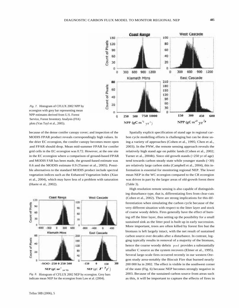
Possibilities for direct validation of large-scale carbon fluxestimates are limited. For NPP, estimates have previously beenmade for 5-yr-average NPP at all plots in the USDA Forest Ser-vice Forest Inventory and Analysis (HA) monitoring networkfor the study area (Van Tuyl et al., 2005). Specific plot locationsare not released for proprietary reasons, so here we comparedthe ecoregion mean value from the FIA data with the distri-bution of CFLUX NPPs for all grid cells containing FIA plotswithin the ecoregion (Fig. 7). The comparisons suggest gener-ally good agreement but a low bias in the CFLUX NPPs forthe WC ecoregion. For NEP, we can compare CFLUX estimateswith those from Law et al. (2004) based on full implementa-tion of the Biome-BGC model over forested cells in the samestudy area (Fig. 8). The land cover, stand age and climate datain Law et al. (2004) were from the same sources but the simu-lation period was the late 1990s and there was no aggregationto 1 km resolution. The comparisons indicate similar sensitivityto differences among the ecoregions and a low bias in the WCecoregion.

4. Discussion

4.1. Model Algorithms

Relatively simple diagnostic carbon cycle models can take ad-vantage of contemporary data from flux towers and remotesensing. However, a significant challenge is to design algorithmsthat are responsive to changing conditions but stable over therange of conditions that might be encountered. Simulating thecarbon cycle in forests is particularly challenging in this regardbecause both fast and slow processes must be accommodated andbecause many forests occur in mountainous terrain with strongenvironmental gradients.

The fast processes are the day-to-day responses to meteoro-logical conditions. The use of the Tmin scalar and VPD scalarsin LUE algorithms such as CFLUX has been shown to be effec-tive over a range of climate regimes (Turner et al., 2005; Turneret al., 2006), especially when calibrated locally and/or supple-mented with information on soil water status (Leuning et al.,1995). Previous work with the MOD17 algorithm used in thestandard MODIS NPP product (Running et al., 2000) has shownthat its lack of responsiveness to overcast conditions frequentlycaused a low bias in the GPP estimates (Turner et al., 2005).The responsiveness to a cloudiness index in CFLUX addressesthis issue, tending to bring LUE up under overcast conditions,which is in line with observations at eddy covariance flux towers(Turner et al., 2003b).

Somewhat slower processes are the regional green-up of non-conifer cover types in the spring, and the soil drought, whichtypically develops over the course of the summer in the PacificNorthwest. Having FPAR in the CFLUX GPP algorithm helpscapture phenology in non-conifer cover types and the inclusionof FPAR in the R h algorithm is supported by measurements of

Tellus 58B (2006), 5


to 235236 to 35

(8

°59 to 670Fig. 5. Net ecosystem production in 2002for the study area. Positive values are carbonsinks.

soil respiration and FPAR or leaf area index in temperate forests(Reichstein et al., 2003) and in clipped grasslands (Wan and Lou,2003). Adding a water balance term to both the GPP and Rh al-gorithms proved to be important in the coniferous forest covertype because soil drought often constrains GPP and Rh in midto late summer in this region (Runyon et at., 1994; Irvine et at.,2002), without change in FPAR. There is of course additional un-certainty introduced by the requirement of specifying WHC andWUE. These variable were treated in a very simplistic mannerfor this initial application of CFLUX but in principle could beaddressed more rigorously with regional soils databases (Kernet at., 1998) and recourse to local eddy covariance flux data forparametrization of WUE (Irvine et at., 2004; Unsworth et at.,2004).

Interannual variation in climate introduces the next scale of

temporal heterogeneity, and in the Pacific Northwest (PNW)is linked in part to the El Nino Southern Oscillation (ENSO)cycle (Greenland, 1994). Studies at eddy covariance flux tow-ers have shown a strong influence of El Niflo years on NEPin the PNW. The 2002-2003 period was largely ENSO neu-tral, but 2003 was generally warmer and wetter over the studyarea. In Douglas-fir dominated forests, years of high temperatureare associated with high ecosystem respiration and decreases inNEP (Morgenstern et al., 2004; Paw U et al., 2004). The resultshere of decreased NEP in 2003 for the CR, WC and KM ecore-gions (predominately Douglas-fir dominated) is consistent withthose observations. In Ponderosa pine dominated forests, waterbalance is probably more important than temperature

Tellus 58B (2006), 5


Change in NEP (gC m -2yr)NM -718 to -226 1185 to 187MO -225 to -123 Ine 188 to 290IN -122 to -20 IM > 290

-19 to 84

Fig. 6. Map of difference in NEP between

2002 and 2003. NEP for 2003 was

subtracted from NEP for 2002. A positivevalue means 2003 was a larger carbon sourceor smaller carbon sink than 2002.

( Kusnierczyk and Ettl, 2002) and at flux towers on Ponderosa

pine sites relatively dry years are associated with lower NPP and

NEP (Law et al., 2000; Mission et al., 2005). That pattern was

seen in this study in the higher NPP and NEP is the EC ecoregion

in 2003.

The very slow carbon cycle processes that must be treated

are the recovery from catastrophic disturbance such as clear-

cuts and fire, and the long-term decrease in NPP over the course

of succession (independent of FPAR). Chronosequence studies

(Acker et al., 2002; Campbell et al., 2004), flux tower studies

(Law et al., 2001), and forest inventory studies (Van Tuyl et al.,

2005) in the Pacific Northwest have all show strong influences

of stand age on NPP and NEP. CFLUX captures the influence of

stand age on NEP by inclusion of scalars derived from outputs

of a model that simulates these long-term trends. Key benefits

of this meta-modelling approach are in retaining the sensitivityto FPAR, which is lost in prognostic models, and avoiding the

computational constraints associated with the Biome-BGC spin-

ups (Thornton et al., 2002), which keeps the model nimble

enough for optimization of multiple parameters.

4.2. Input Data Layers

The MODIS FPAR product has been checked against ground

measurements in only a few cases (Myneni et al., 2002). Over

much of Western Oregon the actual value of FPAR is close to 0.9

Tellus 58B (2006), 5


Coast Range

80

Fig. 7. Histogram of CFLUX 2002 NPP byecoregion with grey bar representing meanNPP estimates derived from U.S. ForestService, Forest Inventory Analysis (FIA)plots (Van Tuyl et al., 2005).

because of the dense conifer canopy cover; and inspection of the

MODIS FPAR product reveals correspondingly high values. In

the drier EC ecoregion, the conifer canopy becomes more open

and FPAR should drop. Mean mid-summer FPAR for conifer

grid cells in the EC ecoregion was 0.72. However, at the one site

in the EC ecoregion where a comparison of ground-based FPAR

and MODIS FAR has been made, the ground-based estimate was

0.6 and the MODIS estimate 0.9 (Turner et al., 2005). Possi-

ble alternatives to the standard MODIS product include spectral

vegetation indices such as the Enhanced Vegetation Index (Xiao

et al., 2004), which may have less of a problem with saturation

(Huete et al., 2002).

-SOO -250 0 250 500 -150 0 150 300

NEP (gC m• syr'I) NEP (gC r yr t )

Fig. 8. Histogram of CFLUX 2002 NEP by ecoregion. Grey barsindicate mean NEP for the ecoregion from Law et al. (2004).

Spatially explicit specification of stand age in regional car-

bon cycle modelling efforts is challenging but can be done us-

ing a variety of approaches (Cohen et al., 1995; Chen et al.,

2003). In the PNW, the remote sensing approach reveals the

relatively high stand age on public lands (Cohen et al., 2002;

Turner et al., 2004b). Since old growth stands (>250 yr of age)

tend towards carbon steady state while younger stands (>30)

are relatively large carbon sinks (Campbell et al., 2004), this in-

formation is essential for monitoring regional NEP. The lower

mean NEP in the WC ecoregion compared to the CR ecoregion

was driven in part by the larger areas of old-growth forest there

(Table 3).

High resolution remote sensing is also capable of distinguish-

ing disturbance type, that is, differentiating fires from clear-cuts(Cohen et al., 2002). There are strong implications for this dif-

ferentiation when simulating the carbon cycle because of the

very different situation with respect to the litter layer and stockof coarse woody debris. Fires generally have the effect of burn-

ing off the litter layer, thus setting up the possibility for a small

sustained sink as the litter pool is built up in early succession.More important, trees are often killed by forest fire but the

biomass is left largely intact, with the net result of sustained

carbon source over decades after a disturbance. In contrast, log-ging typically results in removal of a majority of the biomass,

hence the coarse woody debris pool provides a substantially

smaller C source as the system recovers (Elmer et al., 1995).

Several large-scale fires occurred recently in our western Ore-

gon study area-notably the Biscuit Fire that burned nearly

200 000 ha in 2002. The effect is visible in the southwest corner

of the state (Fig. 6) because NEP becomes strongly negative in

2003. Because of the sustained carbon source from areas such

as this, it will be important to capture the effects of fires in

NPP (gC m "2 yr-1 )

150 300 450 600

NPP (gC m'2 yr 1)Q 250 500 750 1000

Tellus 58B (2006), 5


1.05 -

1.00

0.95 -

0.90 -

0.85 -

0.80 -

0.75 -▪

0.700

(a)

100 200 300 400

Age (yr)

1.1

1.0 -

• 0.9 -

0.8

• 0.7

0.6 -~

0.5 -

0.4 -

0.3 -

0.20

(b)

100 200 300 400

Age (yr)Fig. 9. Stand age effect on (a) gross primary production (y = a + b*exp(c * age)), and (b) heterotrophic respiration (y = a [0.5 + b*exp(c * age) +0.5 (1 - c4e )] for the West Cascades-Evergreen Needleleaf-Clear-cut condition.

Table 3. Means values by ecoregion and year for net primaryproduction (NPP). heterotrophic respiration (Rh ). and netecosystem production (NEP). All units are gC

m_2y

NPP Rh NEP

2002 2003 2002 2003 2002 2003

Ecoregion

Coast Range (CR) 834 732 587 582 246 150Willamette Valley (WV) 716 688 604 626 113 62West Cascades (WC) 611 594 419 433 193 166East Cascades (EC) 350 401 255 270 96 132Klamath Mountains (KM) 737 723 520 551 210 171Regional total 625 606 451 405 174 142

biosphere flux models if they are to ultimately be compared with

flux estimates based on concentration data.

As noted, the aggregation of stand age to the 1 km resolu-

tion had a significant effect on the age distributions, and hence

the NEP estimate. Earlier studies in the PNW have suggested

that a resolution of -250 m is needed to resolve the spatial het-

erogeneity associated with forest management harvesting in this

region (Turner et al., 2000). MODIS has channels for the visible

and near infrared bands at 250 and 500 m resolutions and that

data offers the possibility of more highly resolved FPAR data

that would help address the aggregation problem. Schemes for

weighting the stand age scalar for a given coarse grain grid cell

based on the frequencies of the different ages and their respective

scalar values might also be employed.

Examination of the accuracy of the distributed climate data

was beyond the scope of this study but previous analyses of di-

agnostic NPP models have shown significant impacts of uncer-tainties in distributed climate data on GPP and NPP estimates

(Turner et al., 2005; Zhao et al. 2006). Investigation of issues

associated with the spatial pattern in soil WHC was also not

possible in this analysis but is warranted especially in relation to

si mulating R h .

4.3. Uncertainty in Regional Flux Estimates

Uncertainty in regional flux estimates can be evaluated by com-

parisons to forest plot data and inventory data (Law et al., 2006),by comparisons to products from other models (e.g. Bachelet

et al., 2003), and by checks of observed CO2 concentration

against predicted values when the fluxes are fed into a trans-

port model (Lin et al., 2004).The grid of field plots supported by the USDA HA provided

an opportunity for comparisons of growth rates and here gave an

indication of possible model bias in one of the ecoregions. State-

level estimates of net growth (after accounting for mortality)

from FIA data (e.g. Table 36 in Smith et al., 2004) suggest live

tree carbon is increasing significantly in Oregon in recent years,

even after accounting for harvest removals. This accumulation

is primarily on public lands where harvesting has been greatly

reduced since ^1990. Private lands are approaching an even age

class distribution of stands such that NEP is high because of rapid

tree growth, even though Net Biome Production (Schulze et al.,

2000) is low because much of the stem wood is being removed

by harvesting.

The comparisons of CFLUX products to Biome-BGC outputs

confirmed that the diagnostic model was largely emulating the

results of the prognostic model over forested areas. Flux tower

observations would provide more reliable reference data for op-

timizing the ecophysiological parameters in CFLUX, so it is

desirable that systematic collection of tower data be continued.

As yet, there are no regionally resolved inverse modelling flux

estimates for our study area. It should ultimately be possible

with these analyses to isolate NEP at the regional scale from

the other surface fluxes, notably fossil fuel emissions and directemissions from forest fires. Continental scale inversions report

a large but temporally varying carbon sink in temperate NorthAmerica (Bousquet et al., 2000). The results of this scaling study

Tellus 58B (2006), 5


in the PNW suggest that the region is contributing significantly

to that sink.

5. Conclusions

Spatially and temporally explicit assessments of terrestrial NEP

at the regional scale are needed to understand the influence of

disturbance and climate on carbon flux and for evaluation of fluxestimates based on top down approaches. Because stand age and

disturbance history have significant effects on NPP and R h inforested regions, a bottom-up NEP scaling approach must ide-

ally include such information. Here we developed and tested a

diagnostic NEP model (CFLUX) that accounts for spatial and

temporal patterns in climate and vegetation FPAR, as well as in-

fluences of stand age and disturbance history. With parametriza-

tion at the ecoregion scale based on model runs of Biome-BGC

over a full successional cycle, this monitoring approach captures

the important features of spatial and temporal heterogeneity in

regional NEP. Increased attention is needed to issues related

to the effects of spatial aggregation of model inputs, uncer-

tainty in model parameters and validation of large-scale flux

estimates.

6. Acknowledgments

This research was supported by the NASA Terrestrial Ecology

Program and the U.S. Department of Energy Biological and En-

vironmental Research Terrestrial Carbon Program (Award # DE-

FG02-04ER63917).

7. Appendix A. The Influence of Cloudiness

Observations at flux towers representing a variety of biomes have

commonly found an increase in LUE under overcast conditions,

at both the hourly and daily time steps (Turner et al., 2003b).

To account for this pervasive response, an index of cloudiness

is calculated and allowed to influence the base rate of LUE inCFLUX.

First an index of cloudiness is created based on observed andpotential PAR.

CI = I - (y PAR/ 1, PARpo ),

where

Cl = cloudiness index,

.1.PAR = incident PAR (MJ/d) and4.PAR po = potential incident PAR (MJ/d).

The potential PAR is derived from the algorithm of Fu and

Rich (1999) and actual ,,PAR is from DAYMET.

A cloudiness index scalar is then created in the form:

Sc) = (Cld - Clmin)/(C

lma), - C l

min),

Sct = cloudiness index scalar,

Cl d = cloudiness index for the specific day,

Clm;n = minimum cloudiness index for the year and

CImax = maximum cloudiness index for the year.

The Sc i is then used to determine base LUE for a given day.

e8~ase = (((eg_,n. - eg_cs) * S0 ) + egis)

,

where

eg_basc = base LUE,

eg..ax = maximum LUE, an optimized parameter,

ega.s = clear sky LUE,

Sc i = cloudiness index,

eg.s is calculated as the mean eg for days with STmin = 1 ,

Svp D = 1 and SSwg = I and So < 0.2. This could be from

observations at a flux tower or outputs from a physiologically

based model.

8. Appendix B. Parametrization of age functionsfor GPP and R h

In the case of forested land cover types, the functions specifying

age effects on GPP and R h are calibrated with output from another

model-Biome-BGC (Thornton et at. 2002).

The Biome-BGC model was designed to simulate the carbon

cycle, nitrogen, and hydrologic cycles over the course of pri-

mary and secondary succession and has been extensively tested

in the western Oregon study area (Law et al., 2001, 2004, 2006;

Thornton et al., 2002; Turner et al., 2003a, 2004b). The model is

initially spun-up over an approximately 1000 yr period to bring

the C pools into near steady state. A disturbance event, either

clear-cut (70% of biomass assumed removed) or fire (all forest

floor and 30% of biomass assumed burned off) is then simu-

lated, and the model run forward over the course of secondary

succession with annual outputs of GPP and R h . These data are

normalized to a range of zero to one and then used to fit the age

effect functions (e.g. Figs. 9a and b). GPP/GPPmax is the scalar

for stand age effect on light use efficiency (SsAg ). R h /Rhmax is

the scalar for the stand age effect on heterotrophic respiration

( S snh)•

9. Appendix C. Effects of soil temperature andmoisture on R h

The general formulation of the R h algorithm is:

Rh = Rh_bau * SST * SSW * SSA * FPAR (eq. 6, where)

SST = e(o*Tsoil)

where

Tellus 58B (2006), 5


Tsoil = soil temperature (mean of 24 hr mean air temperature

for previous 25 d),

Sawa = (1 - b * et'swl

)

and SW = proportional soil water content (0-1).

Parametrization of the functions relating soil temperature and

soil water content to R h was based on outputs from Biome-BGC.

The model was first run as in Appendix B and daily outputs forR h , Tsoil, and soil water content for 2002 were saved. The a

parameter was then fit from the relationship of R h to Tsoil, thatis, using Rh = R h_base * S ST . Rh_base was also fit as a free parameter

but not retained. The b and c parameters inSSwh

were then fit

after scaling to a common temperature based on the S ST fit, againwith

Rh_base as a free parameter not retained.

References

Aalto, T., Ciais, P., Chevillard, A. and Moulin, C. 2004. Optimal de-termination of the parameters controlling biospheric C02 fluxes overEurope using eddy covariance fluxes and satellite NDVI measure-ments. Tellus 56B, 93-104.

Acker, S. A., Halpern, C. B., Harmon, M. E. and Dymess, C. T. 2002.Trends in bole biomass accumulation, net primary production andtree mortality in Psuedotsuga rnenziesii forest of contrasting age. TreePhys. 22, 213-217.

Bachelet, O., Neilson, R. P., Hickler, T., Drapek, R. J., Lenihan, J. M.,Sykes, M. T., Smith, B., Stitch, S. and Thonicke, K. 2003. Simulatingpast and future dynamics of natural ecosystems in the United States.Glob. Biogeochem. Cy. 17(1045) doi:10.1029/2001 20019B001508,2003.

Baldocchi, D. D. 2003. Assessing the eddy covariance technique forevaluating carbon dioxide exchange rates of ecosystems: past, presentand future. Glob. Change Biol. 9, 479-492.

Bousquet, P., Peylin, P., Ciais, P., Quere. C. L., Friedlingstein, P. andTans, P P. 2000. Regional changes in carbon dioxide fluxes of landand oceans since 1980. Science 290, 1342-1346.

Campbell, J., Sun, O. J. and Law, B. E. 2004. Disturbance and net ecosys-tem production across three climatically distinct forest landscapes.Global Biogeochem. Cy. 18, GB4017, doi:10.I029/2004GB002236.

Chen, J.1dk, Weimin, J., Cihlar, J., Price, D., Liu, J. and co-authors. 2003.Spatial distribution of carbon sources and sinks in Canada's forests.Tellus 55B, 622-641.

Cohen, W. B., Spies, T. A. and Fiorella, M. 1995. Estimating the age andstructure of forests in a multi-ownership landscape of western Oregon,U.S.A. Int. J. Remote Sens. 16, 721-746.

Cohen, W. B., Spies, T. A., Alig, R. J., Oetter, D. R., Maiersperger,T. K. and co-authors. 2002. Characterizing 23 years (1972-95) ofstand replacement disturbance in western Oregon forests with Landsatimagery. Ecosystems 5, 122-137.

Cohen, W. B., Maiersperger, T. K., Yang, Z., Gower, S. T., Turner, D. P.and co-authors. 2003. Comparisons of land cover and LAl estimatesderived from ETM+ and MODIS for four sites in North America: aquality assessment of 2000/001 provisional MODIS products. RemoteSens. Environ. 88, 233-255.

Cox, P. M., Betts, R. A., Jones, C. D., Spall, S. A. and Totterdell, I. J.2000. Acceleration of global warming due to carbon-cycle feedbacks

in a coupled climate model. Nature 408, 184-187.

Denning, S., Oren, R., McGuire, D., Sabine, C., Doney, S., and co-authors. 2005. Science implementation strategy of the North America

Carbon Program. http://www.carboncyclescience.gov.Falge, E., Baldocchi, E. and Tenhunen, J. 2002. Seasonality of ecosystem

respiration and gross primary production as derived from FLUXNETmeasurements. Agric. Forest Meteorol. 113, 53-74.

Fu, P. and Rich, P. M. (1999). Design and Implementation of the Solar An-alyst: an Arc view extension for modeling solar radiation art lanscapescales. In: Proceedings of the 19th Annual ESRI User Conference, SanDiego, USA. http://gis.esri.com/library/userconf/proc99/proceed/

papers/pap867/p867.htmGreenland, D. 1994. The Pacific Northwest regional context of the cli-

mate of the H.J. Andrews experimental forest. Northwest Sci. 69,81-95.

Hogberg, P., Nordgren, A., Bachmann, N., Taylor, F. S., Ekblad, A.and co-authors. 2001. Large scale forest girdling shows that currentphotosynthesis drives soil respiration. Nature 411, 789-792.

Huete, A., Didan, K., Miura, T., Rodriguez, E. P., Gao, X. and co-authors. 2002. Overview of the radiometric and biophysical perfor-

mance of the MODIS vegetation indices. Retnote Sens. Environ. 83,

195-213.Irvine, J., Law, B. E., Anthoni, P. M. and Meinzer, F. C. 2002. Water

li mitations to carbon exchange in old-growth and young ponderosapine stands. Tree Phys. 22, 189-196.

Irvine, J., Law, B. E., Kurpius, M. R., Anthoni, P. M., Moore, D. and co-authors. 2004. Age-related changes in ecosystem structure and func-tion and effects on water and carbon exchange in ponderosa pine. Tree

Phys. 24, 753-763.Kern, J. S., Turner, D. P. and Dodson, R. F. 1998. Spatial patterns in soil

organic carbon pool size in the Northwestern United States. In: SoilProcesses and the Carbon Cycle (eds.R. Lai, J. M. Kimbal, R. Follett,B. A. Stewart). CRC Press, Boca Raton, FL, 29-43.

Kusnierczyk, E. R. and Ettl, G. J. 2002. Growth response of ponderosa

pine (Pinus ponderosa) to climate in the eastern Cascade Mountains,Washington, U.S.A.: implications for climatic change. Ecoscience 9,

544-551.LaFont, S., Kergoat, L., Dedieu, G., Chevillard, A., Karstens, U. and

Kolle, O. 2002. Spatial and temporal variability in land CO 2 fluxesestimated with remote sensing and analysis over western Eurasia. Tel-lus 54B, 820-833.

Law, B. E., Waring, R. H., Anthoni, P. M. and Aber, J. D. 2000. Mea-surements of gross and net ecosystem productivity and water vaporexchange of a Pinus ponderosa ecosystem, and an evaluation of two

generalized models. Glob. Change Biol. 6, 155-168.Law, B. E., Thornton, P. E., Irvine, J., Anthoni, P. M. and Van Tuyl, S.

2001. Carbon storage and fluxes in ponderosa pine forests at different

development stages. Glob. Change Biol. 7, 1-23.Law, B. E., Falge, E., Gu, L., Baldocchi, D., Bakwin, P. and co-authors.

2002. Environmental controls over carbon dioxide and water vaporexchange of terrestrial vegetation. Agric. Forest Meteorol. 113, 97-120.

Law, B. E., Turner, D., Campbell, J., Van Tuyl, S., Ritts, W. D. and co-authors. 2004. Disturbance and climate effects on carbon stocks andfluxes across Western Oregon USA. Glob. Change Biol. 10, 1429-1444.

Tellus 58B (2006), 5


Law, B. E., Turner, D. P., Lefsky, M., Campbell, J., Guzy, M. and co-authors. 2006. Carbon fluxes across regions: observational constraintsat multiple scale. In: Scaling and Uncertainty Analysis in Ecology:Methods and Applications. (eds. J. Wu, K. B. Jones, H. Li, 0. L.Loucks), Columbia University Press, New York.

Leuning, R., Kelliher, F. M., DePury, D. G. G. and Schultze, E.-D. 1995. Leaf nitrogen, photosynthesis, conductance and transpira-tion: scaling from leaves to canopies. Plant Cell Environ. 18, 1183-1200.

Levy, P. E., Grelle, A., Lindroth, A., Molder, M., Jarvis, P. G. and co-authors. 1999. Regional-scale CO2 fluxes over central Sweden by aboundary layer budget method. Agric. Forest Meteorol. 98-9, 169-180.

Lin, J. C., Gerbig, C., Wofsy, S. C., Andrews, A. E., Daube, B. C.and co-authors. 2004. Measuring fluxes of trace gases at regionalscales by Lagrangian observations: application to the CO2 Budgetand Rectification Airborne (COBRA) studgy. J. Geophys. Res.-Atmos.109 JGR 109 (D15304) doi:10, 10291 2004 JD004754

Mission, L., Tang, J., Xu, M., McKay, M. and Goldstein, A. 2005. In-fluences of recovery from clear-cut, climate variability, and thinningon the carbon balance of a young ponderosa pine plantation. Agric.Forest Meteorol. 130, 207-222.

Montieth, J. L. 1972. Solar radiation and production in tropical ecosys-tems. J. Appl. Ecol. 9, 747-766.

Morgenstern, K., Black, T. A., Humphreys, E. R., Griffis, T. J., Drewitt,G. B. and co-authors. 2004. Sensitivity and uncertainty of the car-bon balance of a Pacific Northwest Douglas-fir forest during an El-Nino/LaNina cycle. Agric. Forest Meteorol. 123, 201-219.

Myneni, R., Hoffman, R., Knyazikhin, Y., Privette, J., Glassy, J. andco-authors. 2002. Global products of vegetation leaf area and fractionabsorbed PAR from one year of MODIS data. Remote Sens. Environ.76, 139-155.

Paw U, K. T., Falk, M., Suchanek, T. H., Ustin, S. L., Chen, J. and co-authors. 2004. Carbon dioxide exchange between an old-growth forestand the atmosphere. Ecosystems 7, 513-524.

Potter, C., Klooster, S., Steinbach, M., Tan, P., Kumar, V. and co-authors.2003. Global teleconnections of climate to terrestrial carbon flux. J.Geophys. Res. 108, doi:10.1029/2002JD002979.

Potter, C. S., Randerson, J. T., Field, C. B., Matson, P. A., Vitousek, P.M. and co-authors. 1993. Terrestrial ecosystem production, a processmodel based on global satellite and surface data. Global Biogeochem.Cy. 7, 811-841.

Prince, S. D. and Goward, S. N. 1995. Global primary production: aremote sensing approach. J. Biogeogr. 22, 815-835.

Raupach, M. R., Rayner, P. J., Barrett, D. J., DefFries, R. S., Heimann,

M. and co-authors. 2005. Model-data synthesis in terrestrial carbonobservation: methods, data requirements and data uncertainty speci-fications. Glob. Change Biol. 11, 378-397.

Reichstein, M., Tenhunen, J., Roupsard, O., Ourcival, J.-M., Rambal, S.

and co-authors. 2003. Inverse modeling of seasonal drought effectson canopy CO 2/H 2 O exchange in three Mediterranean ecosystems. J.Geophys. Res. 108, 1-16.

Running, S. W., Thornton, P. E., Nemani, R. and Glassy, J. M. 2000.Global terrestrial gross and net primary production from the EarthObserving System. In: Methods in Ecosystem Science (eds,O. E. Sala,R. B. Jackson, H. A. Mooney and R. W. Howarth) Springer-Verlag,New York, 44-57.

Runyon, J., Waring, R. H., Goward, S. N. and Welles, J. M. 1994. En-vironmental limits on net primary production and light use efficiency

across the Oregon transect. Ecol. Appl. 4, 226-237.Schimel, D., Melillo, J., Tian, H., McGuire, A. D., Kicklighter, D. and co-

authors. 2000. Contribution of increasing CO 2 and climate to carbonstorage by ecosystems in the United States. Science 287, 2004-2006.

Schulze, E. D., Wirth, C. and Heimann, M. 2000. Managing forests after

Kyoto. Science 289, 2058-2059.Smith, W. B., Miles, P. D., Vissage, J. S. and Pugh, S. A. 2004. Forest

Resources of the United States, 2002. U.S.D.A. Forest Service, North

Central Research Station.Stich, S., Smith, B., Prentice, C. I., Arneth, A., Bondeau, A. and co-

authors. 2003. Evaluation of ecosystem dynamics, plant geography,and terrestrial carbon cycling in the LPJ dynamic global vegetation

model. Glob. Change Biol. 9, 161-185.Thornton, P. E., Running, S. W. and White, M. A. 1997. Generating sur-

faces of daily meteorological variables over large regions of complex

terrain. J. Hydrol. 190, 214-251.Thornton, P. E. and Running, S. W. 1999. An improved algorithm for

estimating incident daily solar radiation from measurements of tem-

perature, humidity, and precipitation.Agric. Forest Meteorol. 93, 211-

228.Thornton, P. E., Hasenauer, H. and White, M. A. 2000. Simultaneous es-

ti mation of daily solar radiation and humidity from observed tempera-ture and precipitation: an application over complex terrain in Austria.

Agric. Forest Meteorol., 255-271.Thornton, P. E., Law, B. E., Gholz, H. L., Clark, K. L., Falge, E. and

co-authors. 2002. Modeling and measuring the effects of disturbancehistory and climate on carbon and water budgets in evergreen needle-leaf forests. Agric. Forest Meteorol. 113, 185-222.

Turner, D. P., Koerper, G. J., Harmon, M. E. and Lee, J. J. 1995. A carbonbudget for forests of the conterminous United States. Ecol. Appl. 5,

421-436.Turner, D. P., Cohen, W. B. and Kennedy, R. E. 2000. Alternative spa-

tial resolutions and estimation of carbon flux over a managed forestlandscape in western Oregon. Land. Ecol. 15, 441-452.

Turner, D. P., Guzy, M., Lefsky, M. A., Van Tuyl, S., Sun, O. and co-authors. 2003a. Effects of land use and fine-scale environmental het-erogeneity on net ecosystem production over a temperate coniferousforest landscape. Tellus 55B, 657-668.

Turner, D. P., Urbanski, S., Wofsy, S. C., Bremer, D. J., Gower, S. T.and co-authors. 2003b. A cross-biome comparison of light use ef-ficiency for gross primary production. Glob. Change Biol. 9, 383-

395.Turner, D. P., Ollinger, S. V. and Kimball, J. S. 2004a. Integrating remote

sensing and ecosystem process models for landscape to regional scaleanalysis of the carbon cycle. BioScience 54, 573-584.

Turner, D. P., Guzy, M., Lefsky, M., Ritts, W., VanTuyl, S. and co-authors. 2004b. Monitoring forest carbon sequestration with remotesensing and carbon cycle modeling. Environmental Manage. 4, 457-

466.Turner, D. P, Ritts, W. D., Cohen, W. B., Maeirsperger, T., Gower,

S. T. and co-authors. 2005. Site-level evaluation of satellite-basedglobal terrestrial gross primary production and net primary productionmonitoring. Glob. Change Biol. 11, 666-684.

Turner, D. P., Ritts, W. D., Zhao, M., Kurc, S. A., Dunn, A. L. and

co-authors. 44: 1899-1907. Assessing interannual variation in

Tellus 58B (2006), 5


MODIS-based estimates of gross primary production. IEEE T Geosci.Remote Sens.

Unsworth, M. H., Phillips, N., Link, T., Bond, B. l., Falk, M. and co-authors. 2004. Components and controls of water flux in an old-growthDouglas-fir-western hemlock ecosystem. Ecosystems 7, 468-481.

Van Tuyl, S., Law, B. E., Turner, D. P. and Gitelman, A. I. 2005. Vari-ability in net primary production and carbon storage in biomass acrossforests-an assessment integrating data from forest inventories, in-tensive sites, and remote sensing. Forest. Ecol. Manag. 209, 273-291.

Wan, S. and Lou, Y. 2003. Substrate regulation of soil respiration in atallgrass prairie: results of a clipping and shading experiment. GlobalBiogeochem. Cy. 17, (1054) doi:10.1029/2002 6B00 1971, 2003.

Waring, R. H. and Running, S. W. 1998. Forest Ecosystems. AcademicPress, San Diego, CA.

White, M. A., Thornton, R E., Running, S. W. and Nemani, R. R. 2000.

Parameterization and sensitivity analysis of the BIOME-BGC terres-trial ecosystem model: net primary productin controls. Earth Interact.

4, 1-85.Xiao, X., Zhang, Q., Braswell, B. H., Urbanski, S., Boles, S. and co-

authors. 2004. Modeling gross primary production of temperate decid-

uous broadleaf forest using satellite images and climate data. Remote

Sens. Environ. 91, 256-270.Yang, Z. 2005. Modeling early forest succession following clear-cutting

in western Oregon. Can. J. For. Res. 35, 1889-1900.Zhao, M. S., Heinsch, F. A., Nemani, R. R. and Running, S. W. 2005. Im-

provements of the MODIS terrestrial gross and net primary productionglobal data set. Remote Sens. Environ. 95, 164-176.

Zhao, M. S., Running, S. W., Nemani, R. R. 2006. Sensitivity of moder-ate resolution imaging spectroradiometer (MODIS) terrestrial primaryproduciton to the accuracy of meteorological reanalysis. J. Geophys.Res. 111(G01002), doi:10:10:1029/2004JGR000004,2006.

Tellus 58B (2006), 5

a diagnostic carbon flux model to monitor the effects of

Documents