a description logic prover in · pdf filea description logic prover in prolog ismail faizi...
TRANSCRIPT

A Description Logic Prover inProlog
Ismail Faizi
Kongens Lyngby 2011IMM-B.Sc.-2011-8

Technical University of DenmarkInformatics and Mathematical ModellingBuilding 321, DK-2800 Kongens Lyngby, DenmarkPhone +45 45253351, Fax +45 [email protected]
IMM-PHD: ISSN 0909-3192

Summary
This work presents development of educational resources for teaching Descrip-tion Logics and reasoning about them using Tableaux algorithms. The start-ing point of this work is the Master thesis of Thomas Herchenroder from theUniversity of Edinburgh. Using Herchenroder’s work and his implementation ofTableaux algorithm for reasoning in ALC , two extensions are developed. One ofthese extensions introduces an alternative ontology format that is more human-friendly compared to the one used by Herchenroder. In addition, a converteris developed that converts expressions between the two formats. The secondextension, Xtableaux.pl, is directly developed on top of the Prolog implemen-tation of Herchenroder, tableaux.pl. This extension is meant to construct theintermediate steps in the proof process. The intention behind this extension isto help students understand the Tableaux algorithms and help in debugging theontology.

ii
Resume
Dette rapport præsenterer udviklingen af uddannelsesresourcer til undervisningaf beskrivelseslogik og ræsonnement omkring dette ved hjælp af Tableaux algo-ritmer. Udgangspunktet for dette arbejde er et speciale af Thomas Herchenroderfra University of Edinburgh. Ved at burge Herchenroder’s arbejde og hans im-plementation af Tableaux algoritmen er der udviklet to udvidelser. En af disseudvidelser indfører en alternativ ontologi format, der er mere menneskevenligei forhold til den, der bruges af Herchenroder. Hertil er der udviklet en kon-verter til at konvertere udtryk mellem de to formater. Den anden udvidelse,Xtableaux.pl, er en direkte udvidelse af Prolog implementationen udviklet afHerchenroder, den sa kaldte tableaux.pl. Denne udvidelse er beregnet til at kon-struere de mellemliggende trins i bevisførelsen. Hensigten bag denne udvidelseer til at hjælpe eleverne med at forsta Tableaux algoritmer og at hjælpe med atfejlfinde ontologier.

iv

Preface
This bachelor project was prepared at Informatics Mathematical Modelling, theTechnical University of Denmark in partial fulfillment of the requirements foracquiring the B.Sc. degree in engineering.
The project deals with development of educational resources for teaching De-scription Logic and reasoning about it using Tableaux algorithm. The mainfocus is based on the work done in a Master thesis about the same topic.
The project consists of both the theoretical aspects of Description Logic and im-plementation of knowledge representation systems based on Description Logic.The work on this project began on 31th of January this year and was completedon 27th of June the same year. This project is credited with 20 ECTS points.
Lyngby, June 2011
Ismail Faizi

vi
Acknowledgements
I thank my supervisors Jørgen Villadsen first by recommanding this projectand second for his constructive ideas and his faith in my abilities to managethis project. It was both enjoyable and easy to work with him.
My heartfelt gratefulness goes to Thomas Herchenroder, whome I have neverseen or have been in contact with in any way, for his great work which I havebased my work on it.
I am grateful to have leaved in the era of researchers like Franz Baader, DiegoCalvanese, Deborah L. MacGuinness, Daneile Nardi, Peter F. Patel-Schneiderand Ian Horrocks. In the words of Isaac Newton “If I have seen further thanothers, it is by standing upon the shoulders of giants.”

viii

Contents
Summary i
Resume iii
Preface v
Acknowledgements vii
1 Introduction 11.1 From Networks to Description Logics . . . . . . . . . . . . . . . . 21.2 DL-based KR Systems . . . . . . . . . . . . . . . . . . . . . . . . 41.3 Application Domains . . . . . . . . . . . . . . . . . . . . . . . . . 51.4 Motivation . . . . . . . . . . . . . . . . . . . . . . . . . . . . . . 51.5 Document Structure . . . . . . . . . . . . . . . . . . . . . . . . . 5
2 Description Logics 72.1 Basic Description Logic . . . . . . . . . . . . . . . . . . . . . . . 72.2 Beyond ALC . . . . . . . . . . . . . . . . . . . . . . . . . . . . . 13
3 Tableaux Algorithm 173.1 Illustration of Tableau-based Algorithms . . . . . . . . . . . . . . 173.2 Overview of Tableaux . . . . . . . . . . . . . . . . . . . . . . . . 193.3 Tableaux Inference Rules . . . . . . . . . . . . . . . . . . . . . . 193.4 Properties of Tableaux . . . . . . . . . . . . . . . . . . . . . . . . 22
4 Implementing the Tableaux Algorithm 254.1 Application of Rules . . . . . . . . . . . . . . . . . . . . . . . . . 264.2 Parsimonious Rules . . . . . . . . . . . . . . . . . . . . . . . . . . 274.3 Keeping the Fringe of the Proof . . . . . . . . . . . . . . . . . . . 30

x CONTENTS
4.4 Handling OR Trees . . . . . . . . . . . . . . . . . . . . . . . . . . 30
5 Specification of the Implemented Tableaux 315.1 Goal Construction . . . . . . . . . . . . . . . . . . . . . . . . . . 325.2 Concept Unfolding . . . . . . . . . . . . . . . . . . . . . . . . . . 335.3 Negative Normal Form . . . . . . . . . . . . . . . . . . . . . . . . 345.4 Expanding the Proof Tree . . . . . . . . . . . . . . . . . . . . . . 35
6 Extending the Tableaux Implementation 416.1 Ontology Format Converter . . . . . . . . . . . . . . . . . . . . . 416.2 Proof Constructor . . . . . . . . . . . . . . . . . . . . . . . . . . 446.3 Testing the Extensions . . . . . . . . . . . . . . . . . . . . . . . . 46
7 Conclusions 497.1 Future Work . . . . . . . . . . . . . . . . . . . . . . . . . . . . . 507.2 Reflection . . . . . . . . . . . . . . . . . . . . . . . . . . . . . . . 50
A Listing of tableaux.pl 51
B Listing of Xtableaux.pl 57
C The Internal Ontology Format 65
D Listing of grammar.pl 67
E Test Data for Proof Constructor 71
F Test Data for Ontology Format Converter 75
G Test Driver Scripts 77G.1 Listing of pc tester.pl . . . . . . . . . . . . . . . . . . . . . . . . 77G.2 Listing of ofc tester.pl . . . . . . . . . . . . . . . . . . . . . . . . 79
References 81

Chapter 1
Introduction
In Artificial Intelligence (AI) one has always been interested in representingknowledge in a manner so it is possible to reason about it, i.e. draw conclusionsfrom the knowledge. The field of the AI which deals with it is KnowledgeRepresentation (KR) and Reasoning.
This field was much popular in 1970s and it was in that time when the de-velopment of approaches to knowledge representations began. These develop-ments are sometimes divided in two categories, logical-based formalisms andnon-logical-based representations. The latter were developed based on networkstructures and rule-based representation – cognitive notions that were derivedfrom experiments on recall from human memory and execution of tasks. Theseapproaches were expected to be more general-purpose, although, they were of-ten developed for specific domains. Unlikely, the logical-based approaches weregeneral-purpose from the beginning since these were a variant of first-order logic(FOL) which provides very powerful and general machinery.
In the logical-based approach, reasoning is equivalent to verifying logical con-sequence, while in the non-logical approaches, it is accomplished by means ofad hoc procedures that manipulate the similarly ad hoc data structures thatare meant to represent the knowledge. Among such representations we havesemantic networks and frames. Both of these can be regarded as network struc-tures where the aim of the network is to represent sets of individuals and their
2 Introduction
Female Person
Woman
Mother Parent
hasChild(1,NIL)
v/r
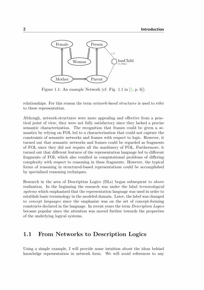
Figure 1.1: An example Network (cf. Fig. 1.1 in [1, p. 6]).
relationships. For this reason the term network-based structures is used to referto these representation.
Although, network-structures were more appealing and effective from a prac-tical point of view, they were not fully satisfactory since they lacked a precisesemantic characterization. The recognition that frames could be given a se-mantics by relying on FOL led to a characterization that could not capture theconstraints of semantic networks and frames with respect to logic. However, itturned out that semantic networks and frames could be regarded as fragmentsof FOL since they did not require all the machinery of FOL. Furthermore, itturned out that different features of the representation language led to differentfragments of FOL which also resulted in computational problems of differingcomplexity with respect to reasoning in these fragments. However, the typicalforms of reasoning in structured-based representations could be accomplishedby specialized reasoning techniques.
Research in the area of Description Logics (DLs) began subsequent to aboverealization. In the beginning the research was under the label terminologicalsystems which emphasized that the representation language was used in order toestablish basic terminology in the modeled domain. Later, the label was changedto concept languages since the emphasize was on the set of concept-formingconstructs declared in the language. In recent years the term Description Logicsbecame popular since the attention was moved further towards the propertiesof the underlying logical systems.
1.1 From Networks to Description Logics
Using a simple example, I will provide some intuition about the ideas behindknowledge representation in network form. We will avoid references to any

1.2 DL-based KR Systems 3
particular system and only speak in terms of a generic network.
A network consists of two elements, nodes and links. The first one is typicallyused to characterize concepts, i.e. sets of individual objects. The latter one isused to characterize relationships among concepts. Here, we will not considerthe knowledge about specific individuals and restrict our attention to knowledgeabout concepts and their relationships.
The simple example, whose pictorial representation is given in figure 1.1 onthe facing page, represents knowledge concerning family relationships. The linkbetween Mother and Parent is a “IS-A” relationship. In this case it means that“mothers are parents”. The IS-A relationship provides the basis for inheritingproperties among the concepts and thus defines a hierarchy over these. Forinstance the concept of Person is a more general concept than the concept ofWoman – if Person has an age so has the Woman.
The ability of DLs to represent relationships beyond the IS-A relationship makesit their characteristic feature. For instance the property called a “role” is one ofthese relationships. The concept of Parent has such property which is expressedby a link to a node labeled hasChild. The role has a so called “value restriction”,denoted by v/r, which puts limitations on the range of types of objects that canfill it. The node has also a number restriction, expressed as (1,NIL), which putsa lower and upper bound on the number of children (NIL denotes infinity). Theconcept of Parent can be read as “A parent is a person having at least onechild, and all of his/her children are persons.” [1, p. 6].
The concept of Mother inherits the restriction on its hasChild role from Parent
since relationships of this kind are inherited from concepts to their subconcepts.There may also be implicit relationships between concepts. For instance, everyMother is a Woman since the concept of Woman is defined as a female person.These kind of inferences are a characterization of the properties of the network.It becomes more difficult to give a precise characterization of what kind of rela-tionships can be computed when the established relationships among conceptsbecomes more complex. Although, a number of systems were implemented andused using the above ideas, the need for a more precise characterization of themeaning of a network emerged. This meaning can be given by defining a lan-guage and by providing an interpretation for the strings of the language [1, p. 7].Such language is given in chapter 2 on page 7.

4 Introduction
KB
TBox
ABox
DescriptionLanguage
Reasoning
ApplicationPrograms Rules
Figure 1.2: Architecture of a DL-based knowledge representation system (cf.Fig. 2.1 in [4, p. 50]).
1.2 DL-based KR Systems
There has been a tight connection between theoretical results and implemen-tation of systems in the research on DL. This has been a characterization ofresearch on DL.
A DL-based KR system provides facilities to set up knowledge bases, to reasonabout their contents and to manipulate them [4, p. 50]. The architecture ofsuch a system is sketched in figure 1.2.
A knowledge base (KB) consists of two components, the TBox and the ABox.The first one introduces the terminology of an application domain, while the sec-ond one contains assertions about named individual in the application domain.These are further described in chapter 2 on page 7.
A DL system is not only a storage place for terminologies and assertions of anapplication domain. The system also offers services that reason about the storedterminologies and assertions. Typical reasoning tasks for TBox and ABox aredescribed in more details in chapter 2 on page 7.
As shown in figure 1.2 a KR system is embedded into a larger environment. Thisis the case in any application. There is an interaction between other componentsand the KR system. These components query the KB and modify it, i.e. addingand retracting concepts, roles and assertions. A restricted mechanism for addingassertions uses rules [4, p. 51]. This notion is beyond the scope of this work andwill not be further mentioned here.

1.3 Application Domains 5
1.3 Application Domains
Description Logics have many application domains. One of the first applicationdomain for DLs was Software engineering where the basic idea was to implementa system that would support the software developer by finding out informationabout a large software system.
One very successful application domain has been configuration. This includesapplications that support the design of complex systems created by combininga number of components, e.g. choosing computer components in order to builda home PC.
There are many other applications domain that have been addressed by the DLcommunity. This work will not further discuss this aspect of Description Logics.For more information one is encouraged to look up [1].
1.4 Motivation
This work is based on a Master thesis of Thomas Herchenroder (from nowon Herchenroder) from the University of Edinburgh. The thesis with the title“Lightweight Semantic Web Oriented Reasoning in Prolog: Tableaux Inferencefor Description Logics” is from 2006.
A large portion of this work has been inspired from Herchenroder’s work. Theimplemented reasoner in Prolog, tableaux.pl, has been used to develop servicesfor better understanding the Tableaux algorithms.
1.5 Document Structure
Chapter 2 is dedicated to discuss the foundation of Description Logics. Inchapter 3 the Tableaux algorithm for reasoning with DLs is introduced. Chapter4 discusses various issues and design alternatives in the implementation of thisalgorithm and presents the implementation introduced by Herchenroder. Inchapter 5, a formal specification of Herchenroder’s implementation is given.Chapter 6 presents the extensions to this implementation and how they aretested. Chapter 7 closes with some conclusions.

6 Introduction

Chapter 2
Description Logics
Description Logic (DL), or Description Logics, is a family of formal knowledgerepresentation languages which has a set-theoretical foundation. Like proposi-tional logic and unlike first-order logic, it has decision procedures. It is, however,more expressive than propositional logic.
DL is used to represent the knowledge of an application domain by definingthe relevant concepts in the domain. And since it is equipped with a formal,logic-based semantics, it is possible to reason about the application domain.
2.1 Basic Description Logic
The basic DL is called Attributive Concept Language with Complements (abbre-viated ALC) [2, p. 2]. It is the basis for the more expressive DLs.
2.1.1 Syntax
In the following I will explain the grammar of the ALC which is shown intable 2.1 on the following page. Before doing so, I will describe the more fun-

8 Description Logics
Concept expression :: ⊥ | > | A | ¬C | CuD | CtD | ∀R.C | ∃R.C
Terminological axiom :: C ≡ D | C v D
Table 2.1: Grammar of the ALC DL [2, p. 8].
damental elements of DL which are common for all DLs. These are presentedin both [2], [4] and [5]. Some of the elements are presented under differentnames among these works, and some are only presented in one or two of thethree works. In the following I will be using the notation of Herchenroder unlessother work is referenced.
In DL there are two kinds of symbols; denoted by atomic symbols. The first oneis the so called atomic concepts (denoted by A,B) and the other one is atomicroles (denoted by R) [4, p. 51].
From the FOL point of view, atomic concepts are unary predicates while atomicroles are binary predicates [4, p. 49]. Beside atomic concepts and atomic roles,DL consists of so called individuals which from FOL point of view are constants.
One can construct arbitrary concept description (denoted by C,D) using atomicsymbols and the so called constructors (concept constructors and role construc-tors). Here, we will only consider concept constructors since ALC only hasatomic roles.
Now back to the grammar of the ALC (see table 2.1). As mentioned earlier,DL has a set-theoretical foundation. This is because the concepts representedin DL are interpreted as sets [2, p. 6]. Looking at grammar for forming conceptexpressions in ALC , one can see that it provides two default concepts denotedby “bottom” (⊥), the empty set, and “top” (>), the universe. These are notfurther defined in the logic, but receive their contents through an interpretation(e.g. model). According to [5], the > concept is an abbreviation for C t ¬C.A concept expression is also an “atomic concept” (A) (also know as primitiveconcept [2, p. 7] or concept name [5, p. 5]).
A concept expression is also one of the “negation” (¬C), “conjunction” (C uD)and/or “disjunction” (C tD). These are the usual Boolean constructors knownin logic. The concept description ¬C means everything that is out side of C;from a set-theoretical point of view it is the complement of C. Like so, theconcept descriptions C uD and C tD mean C ’and’ D and C ’or’ D (logically)respectively. From a set-theoretical point of view it is C intersected with D and

2.1 Basic Description Logic 9
>I = ∆I
⊥I = ∅(¬C)I = ∆I \ CI
(C uD)I = CI ∩DI
(C tD)I = CI ∪DI
(∃R.C)I ={a ∈ ∆I | ∃b. (a, b) ∈ RI ∧ b ∈ CI
}(∀R.C)I =
{a ∈ ∆I | ∀b. (a, b) ∈ RI → b ∈ CI
}(C v D)I = CI ⊆ DI
(C ≡ D)I = CI = DI
Table 2.2: Formal semantic ofALC-concepts and terminological axioms [4, p. 52-53,p. 56] [5, p. 6].
the union of C and D respectively [2, p. 7].
Last but not least, a concept expression is also one of the value restriction(∀R.C) and existential restriction (∃R.C). They are not interpreted the sameway as we know them from FOL. According to Herchenroder , “they describeconcepts as sets of individuals that are characterized by the individuals theyrelate to through a given relation” [2, p. 6]. These are further clarified in sub-section 2.1.2.
2.1.2 Semantics
In the following I describe a formal semantics for ALC concept descriptions andterminological axioms. Such description is given in both [4, p. 52-56] and [5,p. 6].
The formal semantics for the grammar presented in table 2.1 on the precedingpage is given as follows. We consider an interpretation I as a pair (∆I , ·I) wherethe domain (of interpretation) ∆I is a non-empty set and ·I is the interpretationfunction that assigns to every atomic concept A a set AI ⊆ ∆I and to everyatomic role R a binary relation RI ⊆ ∆I×∆I . Figure 2.1 on the following pageillustrate these notions using an extended Venn diagram. Here the text on theleft is matched to the diagram elements on the right using colors.
The interpretation function is extended to the concept descriptions and theterminological axioms presented in table 2.1 on the preceding page. This resultsin inductive definitions shown in table 2.2. In the following I will elaborate on

10 Description Logics
∆IIndividuals: iI ∈ ∆I
John
Mary
Concepts: CI ∈ ∆I
Lawyer
Doctor
Vehicle
Roles: RI ∈ ∆I ×∆I
hasChild
owns
(Lawyer u Doctor)
Figure 2.1: A diagram explaining the semantics of ALC .
two of the definitions from this table; value and existential restriction.
2.1.2.1 Existential Restriction
The interpretation of existential restriction, as it is shown in table 2.2 on theprevious page, is defined as:
(∃R.C)I ={a ∈ ∆I | ∃b. (a, b) ∈ RI ∧ b ∈ CI
}
∆I
CI
(∃R.C)I
RI
iI ∈ ∆I
Figure 2.2: A diagram illustrating the semantics of existential restriction.

2.1 Basic Description Logic 11
∆I
CI
(∀R.C)I
RI
iI ∈ ∆I
Figure 2.3: A diagram illustrating the semantics of value restriction.
In set-theoretical terms it is the set of all individuals (a) that are related throughR to at least one individual (b) from the concept C. This is illustrated by thediagram in figure 2.2 on the facing page where colors match symbols and shapes.For instance the concept CI is represented by a red circle. The individuals inthe domain, i.e. iI ∈ ∆I , are represented using gray dots.
In FOL, the notion of existential restriction is equal to:
∃y.R(x, y) ∧ C(y)
where x is an arbitrary individual in the interpretation domain.
2.1.2.2 Value Restriction
The interpretation of value restriction, as it is shown in table 2.1.2 on page 9,is defined as:
(∀R.C)I ={a ∈ ∆I | ∀b. (a, b) ∈ RI → b ∈ CI
}(2.1)
The FOL equivalent of above is:
∀y.R(x, y)→ C(y)
In set-theoretical terms it is the set of all individuals that are related through(R) to only individuals from the concept (C). This is illustrated by the diagramin figure 2.3. As it is shown in the diagram, individuals out side the domain ofR, i.e. (a, b) /∈ RI , are also in this set. The reason for that is the implication in(2.1). Since the implication is only false when its premise is true, i.e. ¬((a, b) ∈RI)∨ (b ∈ CI), the individuals not in the domain of R will fulfill this, thus theyqualify for being in the set.
12 Description Logics
Woman ≡ Person u FemaleMan ≡ Person u ¬Woman
Mother ≡ Woman u ∃hasChild.PersonFather ≡ Man u ∃hasChild.PersonParent ≡ Father t Mother
GrandMother ≡ Mother u ∃hasChild.ParentMotherWithoutDaughter ≡ Mother u ∀hasChild.¬Woman
Wife ≡ Woman u ∃hasHusband.Man
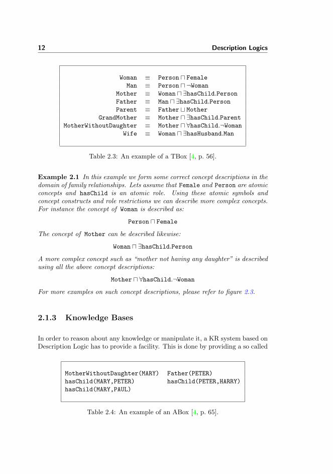
Table 2.3: An example of a TBox [4, p. 56].
Example 2.1 In this example we form some correct concept descriptions in thedomain of family relationships. Lets assume that Female and Person are atomicconcepts and hasChild is an atomic role. Using these atomic symbols andconcept constructs and role restrictions we can describe more complex concepts.For instance the concept of Woman is described as:
Person u Female
The concept of Mother can be described likewise:
Woman u ∃hasChild.Person
A more complex concept such as “mother not having any daughter” is describedusing all the above concept descriptions:
Mother u ∀hasChild.¬Woman
For more examples on such concept descriptions, please refer to figure 2.3.
2.1.3 Knowledge Bases
In order to reason about any knowledge or manipulate it, a KR system based onDescription Logic has to provide a facility. This is done by providing a so called
MotherWithoutDaughter(MARY) Father(PETER)
hasChild(MARY,PETER) hasChild(PETER,HARRY)
hasChild(MARY,PAUL)
Table 2.4: An example of an ABox [4, p. 65].

2.2 Beyond ALC 13
knowledge base or KB. As mentioned earlier, a KB consists of two components,the TBox and the ABox.
2.1.3.1 TBox
The TBox contains the terminology, i.e. the vocabulary of an application domain[4, p. 50]. These are relations such as equivalence (≡) and subsumption (v)between concepts forming terminological axioms. An example of a TBox isgiven in table 2.3 on the facing page.
It is possible to reason about the TBox and not only store terminologies. Typicalreasoning tasks are satisfiability (whether a description is non-contradictory)and subsumption (finding a more general concept).
2.1.3.2 ABox
The ABox contains assertions about concrete individuals in terms of the ter-minology contained in the TBox. These assertions are formed by assigningindividuals (e.g. John, Mary) to concepts (e.g. Parent) or relating them usingroles (e.g. hasChild) in order to describe relations between individuals. Anexample of an ABox is given in table 2.4 on the preceding page.
For ABox, consistency of assertions is an important reasoning problem. Hereone tests whether an assertion has a model, if it is the case then it is consistent[4, p. 50].
In a KB it is very useful to check for satisfiability of descriptions and consistencyof sets of assertions. This way one can determine weather a knowledge base ismeaningful at all. Testing whether a concept is subsumed by another one isalso useful. Doing so, one can organize concepts in hierarchy according to theirgenerality [4, p. 51].
2.2 Beyond ALC
As mentioned earlier, ALC is not very expressive. In order to add expressivenessto DL, the basic Description Logic is extended carefully in order to preserve thegood computational properties. By carefully I mean that not all extensions are
14 Description Logics
(a) Extending with feature X (b) Undecidability
Figure 2.4: Cartoons illustrating that extending DL with feature X would leadto undecidability. The cartoons are taken from [6, p. 21].
good. Some might be harmful and lead to undecidability which is illustratethrough the cartoons in figure 2.4.
Extensions of ALC are indicated by additional letters. For instance the letterN stands for number restrictions (e.g., > 2 hasChild,6 3 hasChild). Addingthis to ALC, we get ALCN which is Attributive Language with Complementsand Number restrictions. Often the letter S is used instead of ALC extendedwith transitive roles (R+) [6, p. 7]. Below is given a list of possible extensionsto ALC. This list is taken from [6, p. 7] and slightly modified.
• H for role hierarchy (e.g., hasDaughter v hasChild)
• O for nominals or singleton classes (e.g., {ITALY})
• I for inverse roles (e.g., isChildOf ≡ hasChild−)
• Q for qualified number restrictions (e.g., > 2 hasChild.Doctor)
• F for functional number restrictions (e.g., 6 1 hasMother)
The complexity of reasoning in the various DLs resulting from extension ofALC can be found using the Complexity Navigator1 of Evgeny Zolin from theUniversity of Manchester.
The basis for W3C’s OWL Web Ontology Language is the so called SHIQDL. This acronym stands for ALC with transitive roles (S), role hierarchy (H),
1http://www.cs.man.ac.uk/ ezolin/dl/

2.2 Beyond ALC 15
inverse roles (I) and qualified number restrictions (Q). Extending SHIQ withnominals (O) results in the so called SHOIQ which is the basis for the OWL DL.Likewise, we have SHIF which is SHIQ with functional restrictions instead ofqualified number restriction. SHIF is the basis for the so called OWL Lite.

16 Description Logics

Chapter 3
Tableaux Algorithm
The DL reasoning algorithms, before the tableau-based algorithms, was the socalled structural subsumption algorithms. These kind of algorithms compare thesyntactic structure of concept descriptions. The problem with these algorithms,although usually being very efficient, is that they are only complete for languagesthat are not so expressive. For instance, these algorithms can not handle DLswith full negation and disjunction [4, p. 81].
With tableau-based algorithms which were first presented for satisfiability ofALC-concepts, it is possible to have interesting hypotheses such as satisfiability,subsumption, equivalence and disjointness. These four kind of hypotheses canbe reduced to only subsumption or unsatisfaibility [2, p. 11]. For instance testingthat C is subsumed by D, i.e. C v D, the formula is rewritten as C u¬D whichis tested for satisfiability. This is possible since a concept C is subsumed byconcept D iff C u ¬D is empty. Testing C v D for satisfiability is not possible.In order to do it, as it is, one has to show that each concept in C is also in D.
3.1 Illustration of Tableau-based Algorithms
Before describing the actual Tableaux inference rules and how these are applied,I illustrate the underlying ideas behind the tableau-based algorithms. This is

18 Tableaux Algorithm
done using a simple example which is presented in [4] on pages 85-86.
Lets assume that we want to know whether
(∃R.A) u (∃R.B) v ∃R.(A uB)
In order to find this out, the query is transformed and the following conceptdescription is created:
C = (∃R.A) u (∃R.B) u ¬∃R.(A uB)
Now, instead of checking for subsumption, above concept description is checkedfor unsatisfaibility. First, all the negation signs are pushed as far as possibleinto the description. This is done using De Morgan’s rules and the usual rulesfor quantifiers. In case of C it means that we obtain:
C0 = (∃R.A) u (∃R.B) u ∀R.(¬A t ¬B)
The above concept description is now in negation normal form. This meansthat only concept names are negated.
Now, we construct a finite interpretation, I, such that CI0 6= ∅, i.e. there mustexist an individual in ∆I (interpretation domain) that is an element of CI0 .
The tableaux algorithm just generates such an element, say b, and imposes theconstraint b ∈ CI0 . This means:
b ∈ (∃R.A)I and b ∈ (∃R.B)I and b ∈ (∀R.(¬A t ¬B))I
From all three constraints, presented above, we can deduce the following. In thecase of b ∈ (∃R.A)I there must exist an individual c such that (b, c) ∈ RI andc ∈ AI . Analogously, in the case of b ∈ (∃R.B)I there must exist an individuald such that (b, d) ∈ RI and d ∈ BI . The two individuals, c and d, are notthe same since “For any existential restriction the algorithm introduces a newindividual as role filler, and this individual must satisfy the constraints expressedby the restriction.” [4, p. 86].
In the case of b ∈ (∀R.(¬A t ¬B))I the individuals from the existential restric-tions are used. This means:
c ∈ (¬A t ¬B)I and d ∈ (¬A t ¬B)I
In order to satisfy c ∈ (¬At¬B)I we can only choose c ∈ (¬B)I since c ∈ (¬A)I
will be in conflict with c ∈ AI from above.

3.2 Overview of Tableaux 19
The same way we can only choose d ∈ (¬A)I in order to satisfy d ∈ (¬At¬B)I
since d ∈ (¬B)I will be in conflict with d ∈ BI from above.
This concludes that C0 is satisfiable since all constraints are satisfiable, i.e.c ∈ AI , (b, c) ∈ RI , d ∈ BI , (b, d) ∈ RI , c ∈ (¬B)I and d ∈ (¬A)I . This meansthat (∃R.A)u (∃R.B) is not subsumed by ∃R.(AuB), since the interpretation,I, is a witness of it. Formally this interpretation is as shown below. This iswhat the tableaux algorithm generated.
∆I = {b, c, d}; RI = {(b, c), (b, d)}; AI = {c}; BI = {d}
This also means that b ∈ ((∃R.A) u (∃R.B))I , but b /∈ (∃R.(A uB))I .
3.2 Overview of Tableaux
Before the tableaux algorithm can start working the DL hypothesis or querymust undergo some transformation. These transformations are:
1. First the goal is constructed. This means that the query is reduced tounsatisfaibility. For instance if the query is C ≡ D the constructed goalis then to show that both (C u ¬D) and (¬C uD) are unsatisfiable.
2. Next, all concepts in the goal are unfolded, i.e. TBox-elimination. Thismeans that all terminological axioms are unfolded such that the goal con-tains only base symbols, i.e. primitive concepts.
3. The goal is written in Negation Normal Form, i.e. all the negations arepushed inwards such that only primitive concepts are negated.
When the transformation steps are completed the tableaux algorithm can startworking. It manipulates the goal by applying four kinds of rules; intersection,union, existential and universal elimination. These rules are shown in table 3.1on the next page and further explained in the following section.
3.3 Tableaux Inference Rules
In this section I give an informal description of each tableaux inference rulepresented in table 3.1 on the following page. These rules are for the basicDL, i.e. ALC. Additional rules for the proof algorithm exists that take care

20 Tableaux Algorithm
u – rule if 1. (C1 u C2) ∈ L(x)2. {C1, C2} * L(x)
then L(x) −→ L(x) ∪ {C1, C2}t – rule if 1. (C1 t C2) ∈ L(x)
2. {C1, C2} ∩ L(x) =then L(x) −→ L(x) ∪ {C1, C2}
a. save Tb. try L(x) −→ L(x) ∪ {C1}
If that leads to a clash then restore T andc. try L(x) −→ L(x) ∪ {C2}
∃ – rule if 1. ∃R.C ∈ L(x)2. there is no y s.t. L(〈x, y〉) = R and C ∈ L(y)
then create a new node y and edge 〈x, y〉with L(y) = C and L(〈x, y〉) = R
∀ – rule if 1. ∀R.C ∈ L(x)2. there is some y s.t. L(〈x, y〉) = R and C /∈ L(y)
then L(y) −→ L(y) ∪ C
Table 3.1: Tableaux Inference Rules for ALC [2, p. 14].
of the additional operators and constructors added to the language. For moreinformation on this subject please refer to [1].
The notions C, C1 and C2 in table 3.1 denote arbitrary DL concepts. A relationis represented by R. The whole proof tree is represented by T, while x and ydenote specific nodes in the tree. The set of DL formulas associated with a nodex is denote by L(x) (node label).
Each rule in table 3.1 consists of two parts, an precondition part (the if part) andan action part (the then part). The precondition part consists of two conditionsthat both must be satisfied in order for the action part to take effect. The firstcondition is always a check for the presence of the term in the node label, whilethe second one is usually a check for the result not already being presence inthe node label.
The first rule (denoted u–rule) is applied to intersection terms within a givennode label. The second condition makes sure that both of the operands are notalready presence in the node label. In the action part, both operands are addedas new members to the current node label.
The second rule (denoted t–rule) is applied to union terms within a given nodelabel. The second condition of this rule makes sure that none of the operandsare already in the node label. The action part consists of three steps. In the first
3.3 Tableaux Inference Rules 21
step the whole tree (denoted T) is saved. In the second step, the first operandof the union term is added to the current node label and the proof procedureproceeds. If this instance of the tree lead to a clash then the tree is restored. Instep three the second operand is added to the just restored tree and the proofprocedure is proceeded.
The third rule (denoted ∃–rule) is applied to the existential restriction terms(∃R.C) in a given node label. The second condition in this rule makes sure thata node with the same relation (R) as edge label and containing the constrainedconcept (C) does not already exist. If this is not the case, such a node is created.
The last rule in table 3.1 on the preceding page (denoted ∀–rule) is applied tothe value restriction terms. In this rule, the second condition makes sure that anode having the relation as the edge label and not containing the constrainingconcept exist. If this is the case, the constraining concept is added to the nodelabel of that node.
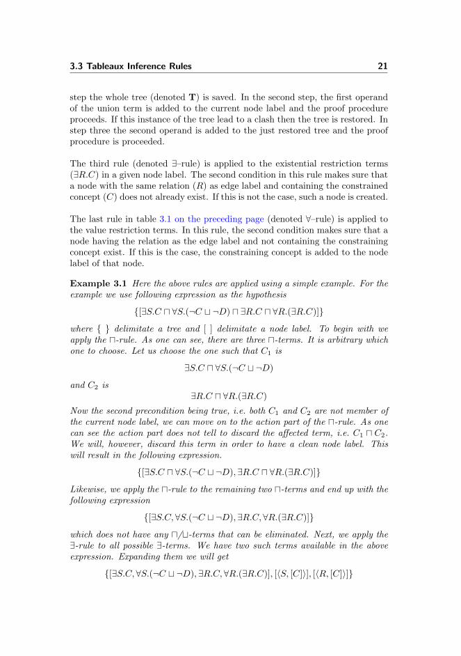
Example 3.1 Here the above rules are applied using a simple example. For theexample we use following expression as the hypothesis
{[∃S.C u ∀S.(¬C t ¬D) u ∃R.C u ∀R.(∃R.C)]}
where { } delimitate a tree and [ ] delimitate a node label. To begin with weapply the u-rule. As one can see, there are three u-terms. It is arbitrary whichone to choose. Let us choose the one such that C1 is
∃S.C u ∀S.(¬C t ¬D)
and C2 is∃R.C u ∀R.(∃R.C)
Now the second precondition being true, i.e. both C1 and C2 are not member ofthe current node label, we can move on to the action part of the u-rule. As onecan see the action part does not tell to discard the affected term, i.e. C1 u C2.We will, however, discard this term in order to have a clean node label. Thiswill result in the following expression.
{[∃S.C u ∀S.(¬C t ¬D),∃R.C u ∀R.(∃R.C)]}
Likewise, we apply the u-rule to the remaining two u-terms and end up with thefollowing expression
{[∃S.C, ∀S.(¬C t ¬D),∃R.C,∀R.(∃R.C)]}
which does not have any u/t-terms that can be eliminated. Next, we apply the∃-rule to all possible ∃-terms. We have two such terms available in the aboveexpression. Expanding them we will get
{[∃S.C,∀S.(¬C t ¬D),∃R.C,∀R.(∃R.C)], [〈S, [C]〉], [〈R, [C]〉]}

22 Tableaux Algorithm
where 〈R,C〉 represents the expansion of a ∃-term with R being the edge and Cthe new created node. Next, we expand all possible ∀-terms. There are two ofsuch terms which result in
{[∃S.C,∀S.(¬Ct¬D),∃R.C,∀R.(∃R.C)], [〈S, [C,¬Ct¬D]〉], [〈R, [C, ∃R.C]〉]}
which is the result of adding the concept of each ∀-term to the node having therole as the edge. The two new nodes that resulted from the expansion of ∃- and∀-terms are taken as the current nodes, i.e. the nodes that the proof rules areapplied to. We have following current nodes:
{[C,¬C t ¬D], [C,∃R.C]}
The same way as above, the proof rules are applied to the above nodes one byone. We apply the t-rule to the first node and get
{[C,¬C], [C,∃R.C]}L{[C,¬D], [C,∃R.C]}R
where we have two trees labeled L (left) and R (right). We proceed with the lefttree and immediately realise that there is a clash, C and ¬C, which closes thisbranch of the Tableaux. The rest of the proof is left for the reader to complete.We can already conclude that the hypothesis is unsatisfiable since we already hada clash on one of the branches of the Tableaux.
3.4 Properties of Tableaux
According to Herchenroder [2, p. 16], the tableaux algorithm presented in ta-ble 3.1 on page 20 is sound and complete. It will also always terminate usingexponential time and space complexity.
The termination property is derived from the fact that the algorithm only addssubexpressions that are strictly smaller than the parent expressions. There isalways a limited number of these expressions, since the initial expression is finite.The branching and depth of the proof tree is also limited, since this depends onthe number of existential in the initial formula, which again is limited. Moreover,the rules conditions are there to prevent loops in expanding terms [2, p. 16].
According to Herchenroder, soundness and completeness rely on the equivalenceof the satisfiability of the initial formula and the consistency of the saturatedproof trees. This can be shown partly using a canonical model and takingadvantage of the finite tree model property.

3.4 Properties of Tableaux 23
Regarding the complexity of the algorithm, it is exponential in time and spacein worst-case [2, p. 16].

24 Tableaux Algorithm

Chapter 4
Implementing the TableauxAlgorithm
In this chapter, I will present the design and implementation decisions madein [2] in order to implement a more efficient implementation with regards tomemory consumption and runtime. These decisions are:
• Applying tableaux rules in order instead of randomly.
• Replacing terms by their rule derivatives instead of keeping both.
• Instead of keeping the whole proof tree only the fringe of the proof is keptduring the proof procedure.
• When eliminating union (t) a choice point is made and the resulting treesare explored sequentially instead of concurrently.
These decisions are explained more thorough in the following.
26 Implementing the Tableaux Algorithm
4.1 Application of Rules
Although the original definition of the Tableaux algorithm does not suggestany thing about the order of the application of rules, it is of great importanceand provides significant advantages in a concrete implementation. As shown byBaader and Sattler (cf. [2]) it reduces the worst-case space requirements of thealgorithm to polynomial.
The modified algorithm stated by Herchenroder operates in iteration consistingof two steps. These steps are first applied to the goal, denoted C0(x0). In stepone the u- and t-rules are applied as long as possible and the node is checkedfor clashes. In the second step the algorithm generates all the direct successorsof x0 using the ∃-rule and thoroughly applies the ∀-rule to the correspondingrole assertions. The algorithm continues by applying step one and two to thesuccessors in the same way.
This section summarizes the discussion of Herchenroder regarding this approach.I have used his example in order to make the arguments obvious.
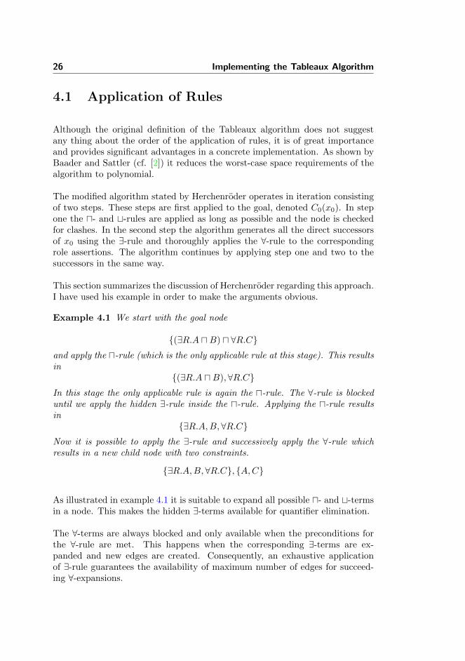
Example 4.1 We start with the goal node
{(∃R.A uB) u ∀R.C}and apply the u-rule (which is the only applicable rule at this stage). This resultsin
{(∃R.A uB),∀R.C}In this stage the only applicable rule is again the u-rule. The ∀-rule is blockeduntil we apply the hidden ∃-rule inside the u-rule. Applying the u-rule resultsin
{∃R.A,B, ∀R.C}Now it is possible to apply the ∃-rule and successively apply the ∀-rule whichresults in a new child node with two constraints.
{∃R.A,B,∀R.C}, {A,C}
As illustrated in example 4.1 it is suitable to expand all possible u- and t-termsin a node. This makes the hidden ∃-terms available for quantifier elimination.
The ∀-terms are always blocked and only available when the preconditions forthe ∀-rule are met. This happens when the corresponding ∃-terms are ex-panded and new edges are created. Consequently, an exhaustive applicationof ∃-rule guarantees the availability of maximum number of edges for succeed-ing ∀-expansions.

4.2 Parsimonious Rules 27
u – rule if 1. (C1 u C2) ∈ L(x)2. {C1, C2} * L(x)
then L(x) −→ (L(x) \ (C1 u C2)) ∪ {C1, C2}t – rule if 1. (C1 t C2) ∈ L(x)
2. {C1, C2} ∩ L(x) =then L(x) −→ L(x) ∪ {C1, C2}
a. save Tb. try L(x) −→ (L(x) \ (C1 t C2)) ∪ {C1}
If that leads to a clash then restore T andc. try L(x) −→ (L(x) \ (C1 t C2)) ∪ {C2}
∃ – rule if 1. ∃R.C ∈ L(x)2. there is no y s.t. L(〈x, y〉) = R and C ∈ L(y)
then create a new node y and edge 〈x, y〉with L(y) = C and L(〈x, y〉) = R andL(x) −→ L(x) \ ∃R.C
∀ – rule if 1. ∀R.C ∈ L(x)2. there is some y s.t. L(〈x, y〉) = R and C /∈ L(y)
then L(y) −→ L(y) ∪ C for every applicable y andL(x) −→ L(x) \ ∀R.C
Table 4.1: Modified Tableaux Inference Rules for ALC. Taken from [2, p. 14].
4.2 Parsimonious Rules
The ordered and exhaustive application of the tableaux inference rules to theDL expressions of a node label as discussed above makes it possible to deducethe so called Parsimonious Rules. According to Herchenroder these rules makesit possible to kill to birds with one stone. This means that parsimonious rulesnot only remove the redundant information from the proof tree and only keepthe derivative terms, but also makes some of the preconditions for the originalrules superfluous.
In this section I present the parsimonious rules derived by Herchenroder in [2,p. 24-29].
4.2.1 Replacement of Expressions by their Derivatives
In the standard tableaux algorithm the derivatives of the expressions are justadded to the corresponding node label and new child nodes are added to theproof tree. This is shown in example 4.2 on the following page (cf. [2, p. 24]).
28 Implementing the Tableaux Algorithm
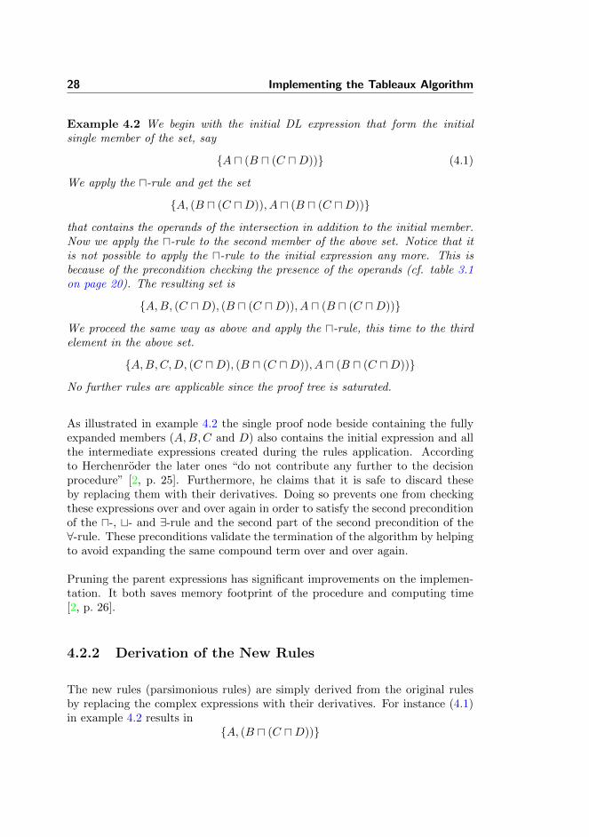
Example 4.2 We begin with the initial DL expression that form the initialsingle member of the set, say
{A u (B u (C uD))} (4.1)
We apply the u-rule and get the set
{A, (B u (C uD)), A u (B u (C uD))}
that contains the operands of the intersection in addition to the initial member.Now we apply the u-rule to the second member of the above set. Notice that itis not possible to apply the u-rule to the initial expression any more. This isbecause of the precondition checking the presence of the operands (cf. table 3.1on page 20). The resulting set is
{A,B, (C uD), (B u (C uD)), A u (B u (C uD))}
We proceed the same way as above and apply the u-rule, this time to the thirdelement in the above set.
{A,B,C,D, (C uD), (B u (C uD)), A u (B u (C uD))}
No further rules are applicable since the proof tree is saturated.
As illustrated in example 4.2 the single proof node beside containing the fullyexpanded members (A,B,C and D) also contains the initial expression and allthe intermediate expressions created during the rules application. Accordingto Herchenroder the later ones “do not contribute any further to the decisionprocedure” [2, p. 25]. Furthermore, he claims that it is safe to discard theseby replacing them with their derivatives. Doing so prevents one from checkingthese expressions over and over again in order to satisfy the second preconditionof the u-, t- and ∃-rule and the second part of the second precondition of the∀-rule. These preconditions validate the termination of the algorithm by helpingto avoid expanding the same compound term over and over again.
Pruning the parent expressions has significant improvements on the implemen-tation. It both saves memory footprint of the procedure and computing time[2, p. 26].
4.2.2 Derivation of the New Rules
The new rules (parsimonious rules) are simply derived from the original rulesby replacing the complex expressions with their derivatives. For instance (4.1)in example 4.2 results in
{A, (B u (C uD))}

4.2 Parsimonious Rules 29
after applying the u-rule.
Formally this is done as follows (cf. [2, p. 25])
L(x) −→ (L(x) \ (C1 u C2)) ∪ {C1, C2}
which means that the parent term is removed from the node label (expressedby the “\” operator) before the derivative of a rule application is added to thenode label (expressed by the “∪” operator). Table 4.1 on page 27 presents thecomplete list of the modified rules.
Now the question is whether pruning of the parent expressions alter the seman-tics of the node label? Moreover, whether it renders the node empty? Accordingto Herchenroder neither is the case [2, p. 27-29]. In the following I will presenta summary of his argumentation.
In the case of u-expansion pruning the parent expression does not change thesemantics of the node label. This is due do the equivalence of sets {A,B} and{AuB} semantically. In the set {A,B,AuB} the parent expression (AuB) justrestates the requirement that individuals must satisfy A and B and is thereforeredundant. The node label is not possible to render empty after removing theparent term, since the set will contain the operands of the term after the ruleapplication.
The same holds in the case of t-expansion. Here the tree is duplicated and eachoperand of the complex t-term is added to the node label in each of the trees.This preserves fully the semantics of the t-term, since it is only satisfiable ifeither there exists a model fulfilling the tree with the first operand, or a modelfor the tree with second operand. Put in other words, the term does not add anew constraint to the respective node label, and is therefore redundant and canbe discarded. The node label can not be rendered empty, since there will existsan operand after the rule application.
In the case of ∃-terms a new child node, containing the concept name, is createdand new edge to it, with the name of the relation as the label, is added. This fullypreserves the initial semantics of the ∃-term. Keeping the term is only retainingredundant information. While removing the term will result in prohibition offurther expansion of it. It is also possible to render the node label empty byremoving the term, but it is harmless, since the child node contains the relevantinformation in order to continue the decision procedure.
The same holds in the case of ∀-terms (∀R.C). There is a possibility to renderthe node label empty by pruning the term, but it is harmless because of thesame reason as mentioned above. It can, however, be damaging to the proof

30 Implementing the Tableaux Algorithm
to prune the term. It is due to the fact that a ∀-term can be evaluated oncefor each existing child node with matching relation (R) edge and non-existentconcept C. Therefore, we must make sure that it is maximally applied and thenprune it from the node label.
4.3 Keeping the Fringe of the Proof
Analogous to complex DL expressions which can be pruned from the node label,once the rule is applied, the whole node can also be discarded, once it has beenexhaustively transformed and expanded, checked for clashes and its all possiblechild nodes have been derived with their labels fully expanded. Therefore, it issufficient only to keep track of the current set of leaf nodes, or better known asfringe [2, p. 30], instead of always maintaining the whole tree.
According to Herchenroder, keeping only the fringe of the proof tree providessome advantages without having any negative effects [2, p. 30]. One of theseadvantages is the need for less memory.
He also mentions that parent node must be fully expanded before it can bediscarded. The expansion is both in terms of child expansion and clash detection.
4.4 Handling OR Trees
One has to make non-deterministic choice every time a t-connective has to beexpanded. This leaves room for implementation variants. In his implementation,Herchenroder has chosen the sequential version of exploring t-trees. This is,every time a t-term has to be expanded, the proof tree containing the firstoperand of the term is explored until it fails. On failure, the proof tree containingthe second operand of the term is explored in order to get a model.
An alternative way, is exploring the trees concurrently. This is, exploringthe proof tree with the first operand and its duplicates containing the secondoperand simultaneously.
According to Herchenroder , the sequential version not only saves runtime mem-ory, but is also a very attractive solution when developing with Prolog, since itfits naturally into Prolog’s backtracking strategy.

Chapter 5
Specification of theImplemented Tableaux
In this chapter, I summarize the specification of the tableaux.pl, the implementa-tion of tableaux algorithm proposed by Herchenroder. This chapter is basicallythe summary of chapter 5 in [2] with the addition of the running example thatI have constructed by myself.
As mentioned in chapter 3 on page 17, the DL query must undergo some trans-formation before the actual Tableaux algorithm can start working. The firststep in the transformation process is the construction of the goal [2, p. 34]. Thecomplex DL concepts in the goal are replaced by their definition in order toconstruct an expression that only contains atomic concepts. This step of trans-formation is called concept unfolding [2, p. 35]. The resulting DL expressionis now transformed into so called Negative Normal Form where the negationsare pushed inwards until only the atomic concepts are negated. The actualproof starts with the result of this transformation by first eliminating the u-and t-connectives and then checking for clashes. Next, all possible ∃-terms areexpanded and the corresponding (with the same relation) ∀-terms are applied.The process is then repeated for the resulting child nodes.
In the following sections I describe the above process and the specification ofthe tableaux.pl thoroughly and with use of a running example. This example
32 Specification of the Implemented Tableaux
is constructed by querying the ontology (TBox) shown in table 2.3 on page 12.The specific query is
MotherWithoutDaughter v Mother (5.1)
which means that the concept of MotherWithoutDaughter is subsumed by theconcept of Mother, i.e. the concept of Mother is a more general concept thenthe concept of MotherWithoutDaughter.
In order to list the specification of certain predicates, I use the notation usedby Herchenroder in his description. The capital letters A,B,C, . . . denote well-formed DL concept expressions. On the left of the arrow (←) are goals thatmust be satisfied, while on the right of it are the subgoals that will allow oneto derive the main goal if they are satisfiable. Predicates with two parameters,e.g. nnf (A,B), can be understood as taking the first parameter (A) as inputand constructing the second one (B) as output.
5.1 Goal Construction
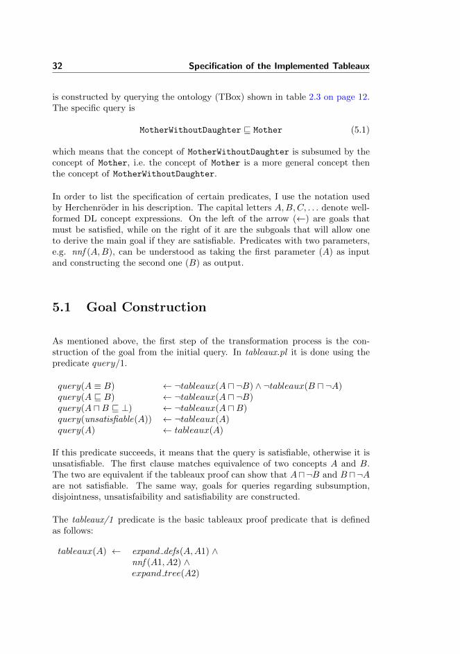
As mentioned above, the first step of the transformation process is the con-struction of the goal from the initial query. In tableaux.pl it is done using thepredicate query/1.
query(A ≡ B) ← ¬tableaux(A u ¬B) ∧ ¬tableaux(B u ¬A)query(A v B) ← ¬tableaux(A u ¬B)query(A uB v ⊥) ← ¬tableaux(A uB)query(unsatisfiable(A)) ← ¬tableaux(A)query(A) ← tableaux(A)
If this predicate succeeds, it means that the query is satisfiable, otherwise it isunsatisfiable. The first clause matches equivalence of two concepts A and B.The two are equivalent if the tableaux proof can show that Au¬B and B u¬Aare not satisfiable. The same way, goals for queries regarding subsumption,disjointness, unsatisfaibility and satisfiability are constructed.
The tableaux/1 predicate is the basic tableaux proof predicate that is definedas follows:
tableaux(A) ← expand defs(A,A1) ∧nnf (A1, A2) ∧expand tree(A2)

5.2 Concept Unfolding 33
The three subgoals (expand defs(A,A1), nnf (A1, A2) and expand tree(A2))which this predicate consists of, are the transformation of the goal and the ac-tual proof procedure. Concept unfolding is done by the predicate expand defs/2,while transforming the goal to Negative Normal Form is done by the predicatennf /2. The expand tree/1 predicate is the actual proof procedure which trans-forms and expands the initial node by well-defined proof steps. The goal failsif possible clashes are inspected during the expansion of the tree. If no clashesare detected when the tree is fully expanded, the goal succeeds.
Example 5.1 This example is the first example in a series of examples illus-trating the specification of the tableaux.pl. In this example we construct thegoal for (5.1). The goal becomes
MotherWithoutDaughter u ¬Mother (5.2)
according to the second clause of query/1. If the tableaux proof can show thatthe above expression is not satisfiable then (5.1) is true, otherwise it is false.
In the following section we proceed with concept unfolding or expansion of thegoal expression.
5.2 Concept Unfolding
In this step of the transformation all the so called name concepts that aredefined in terms of other concepts are replaced by their definition. For instancethe name concept Mother in the goal constructed in example 5.1 is replaced byits definition
Woman u ∃hasChild.Person (5.3)
which is given in table 2.3 on page 12. In tableaux.pl this is done using theexpand defs/2 predicate which is defined as:
expand defs(A,A1) ← atomic(A) ∧ ont(equiv(A,A2)) ∧ expand defs(A2, A1)expand defs(A,A1) ← atomic(A) ∧ ¬ont(equive(A, ))
The definition states that each atomic concept A in the ontology is replaced bythe expression in the right side of the ≡ (equiv/2). Concept names which donot have a definition in the ontology are returned as primitives. This is appliedrecursively until the whole expression is unfolded.
Example 5.2 This example is the second example in the series of examplesillustrating the specification of the tableaux.pl. In this example we unfold thename concepts in (5.2) from example 5.1.

34 Specification of the Implemented Tableaux
We are concerned with two name concepts. These are MotherWithoutDaughter
and Mother. If we begin with the second name concept and replace it with itsdefinition, we will get (5.3) which contains a name concept, Woman. Replacingit will result in the fully expanded DL concept that we called Mother.
The concept MotherWithoutDaughter can be expanded in the same way. Thegoal will then become a very long expression which is not suited to be presentedhere. Therefore, only the first letter of each concept ( P for Person and F forFemale) is presented and the role hasChild is replaced by the letter R. Thefully expanded goal is than given as follows:
((P u F) u ∃R.P u ∀R.(¬(P u F))) u ¬((P u F) u ∃R.P) (5.4)
In the following section we proceed by pushing all the negation in the goalinwards such that only primitive concepts are negated.
5.3 Negative Normal Form
In order for the tableaux proof procedure to begin, the goal must undergo onelast transformation. All the negations must be pushed inside such that onlyprimitive concepts are negated. After this transformation the goal will be innegation normal form. In the tableaux.pl this transformation is done by thepredicate nnf /2 which is defined as follows:
nnf (¬¬C,C)nnf (¬∀R.C,∃R.C1) ← nnf (¬C,C1)nnf (∀R.C,∀R.C1) ← nnf (C,C1)nnf (¬∃R.C,∀R.C1) ← nnf (¬C,C1)nnf (∃R.C,∃R.C1) ← nnf (C,C1)nnf (¬(A uB), A1 tB1) ← nnf (¬A,A1) ∧ nnf (¬B,B1)nnf (A uB,A1 uB1) ← nnf (A,A1) ∧ nnf (B,B1)nnf (¬(A tB), A1 uB1) ← nnf (¬A,A1) ∧ nnf (¬B,B1)nnf (A tB,A1 tB1) ← nnf (A,A1) ∧ nnf (B,B1)nnf (¬C,¬C) ← atomic(C)nnf (C,C) ← atomic(C)
As one can see the above clauses apply the rules such as ¬¬C ≡ C, ¬∀R.C ≡∃R.¬C, De Morgan’s laws etc. These rules are applied recursively until onlythe primitive concepts are negated.

5.4 Expanding the Proof Tree 35
Example 5.3 This example is the third example in the series of examples illus-trating the specification of the tableaux.pl. In this example we transform (5.4)from example 5.2 on page 33 into negative normal form.
There are two concepts that are negated in (5.4). These are ¬(PuF) and ¬((PuF)u∃R.P). The first concept is transformed into negative normal form using DeMorgan’s rules and we get (¬Pt¬F). The second concept is more complex thanthe first one. Here we must apply De Morgan’s twice and beside that also therule ¬∃R.C ≡ ∀R.¬C. This results in ((¬P t ¬F) t ∀R.(¬P)). The goal is nowtransformed into negative normal form and looks like shown below.
((P u F) u ∃R.P u ∀R.(¬P t ¬F)) u ((¬P t ¬F) t ∀R.(¬P)) (5.5)
It is now ready to be processed by the tableaux proof procedure.
In the following section we proceed with the actual tableaux proof procedurewhere the goal is expanded/transformed using the tableaux inference rules.
5.4 Expanding the Proof Tree
When the goal has been transformed such that all concepts names are replacedby their most basic definitions and all negations are pushed inwards such thatonly primitive concepts are negated, the tableaux proof procedure starts work-ing. The procedure expands the tree in a standard agenda-style tree expansion[2, p. 36] where leaf nodes are examined, transformed (u- and t-elimination) orexpanded (∃- and ∀-expansion) and the resulting node(s) are put back into thelist of current fringe nodes for further examination [2, p. 36].
In the tableaux.pl this process starts with the basic predicate, process node/2,that is defined as follows:
process node(A,B) ← transform connectives(A,A1) ∧expand node(A1, B)
This predicate works on a single node from the proof tree. First all the u/t-connectives are eliminated using the transform connectives/2 and next the trans-formed node is expanded by possible ∃/∀-expansion using the expand node/2predicate.
The transform connectives/2 predicate basically applies the u- and t-rule re-cursively to all u- and t-terms. This predicate is defined as follows:

36 Specification of the Implemented Tableaux
transform connectives([A uB|R], R1) ←transform connectives([A,B|R], R1)
transform connectives([A tB|R], R1) ←transform connectives([A|R], R1) ∧transform connectives([B|R], R1)
The expand node/2 predicate first checks for possible clashes in the just trans-formed node. Its core is, however, the expansion of the ∃ and ∀ quantifiers. Thedefinition of this predicate is given below.
expand node(N, ) ← check clash(N)expand node(N,NL) ← expand exist(N, [], E) ∧
expand univ(N,E,NL)
Example 5.4 This example is the fourth example in the series of examplesillustrating the specification of the tableaux.pl. In this example we eliminateall the possible u- and t-connectives in (5.5) from example 5.3 on page 34. Theinitial tree where the proof procedure starts is presented below.{
[((P u F) u ∃R.P u ∀R.(¬P t ¬F)) u ((¬P t ¬F) t ∀R.(¬P))]}
where { } and [ ] delimit trees and nodes in a tree, respectively. In the above treethere is only one node. This node has four u-terms which all can be eliminated.The result is {
[P, F,∃R.P,∀R.(¬P t ¬F), ((¬P t ¬F) t ∀R.(¬P))]}
which can be further transformed by eliminating the possible t-connectives. Inthe above node there are two of such connectives. The elimination of first ofthese connectives result in the following:{
[P, F,∃R.P,∀R.(¬P t ¬F), (¬P t ¬F)]}L{
[P, F,∃R.P,∀R.(¬P t ¬F),∀R.(¬P)]}R
(5.6a)
The whole tree is duplicated and the t-term is pruned from the only node inthe tree and the left operand of the t-term is added to the first copy of the treeconstructing the left tree (denoted by L), while the right operand is added to thesecond copy of the tree constructing the right tree (denoted by R). It is here achoice point is made and the proof procedure is proceeded using one of the treesand upon failure the alternative is tried. In his implementation Herchenroderproceeds with the left tree first and on failure the right tree is processed. We willproceed the same way.
The left tree is now transformed the same way as the initial tree— the u/t-connectives are eliminated. In the left tree there is only one node which consists
5.4 Expanding the Proof Tree 37
of only one t-term that can be transformed— the other t-term is in the scopeof the value restriction and can only be transformed after the expansion of the∀. We get again two trees:{
[P, F,∃R.P,∀R.(¬P t ¬F),¬P]}LL
(5.7a){[P, F,∃R.P,∀R.(¬P t ¬F),¬F]
}LR
(5.7b)
Likewise, we have a choice point here. But here we notice that both nodes in thetwo trees contains clashes (P, ¬P in (5.7a) and F, ¬F in (5.7b)) and thus bothare closed.
We return back to the first choice point and proceed with the right tree (see(5.6a)). This is done in example 5.5 on the following page.
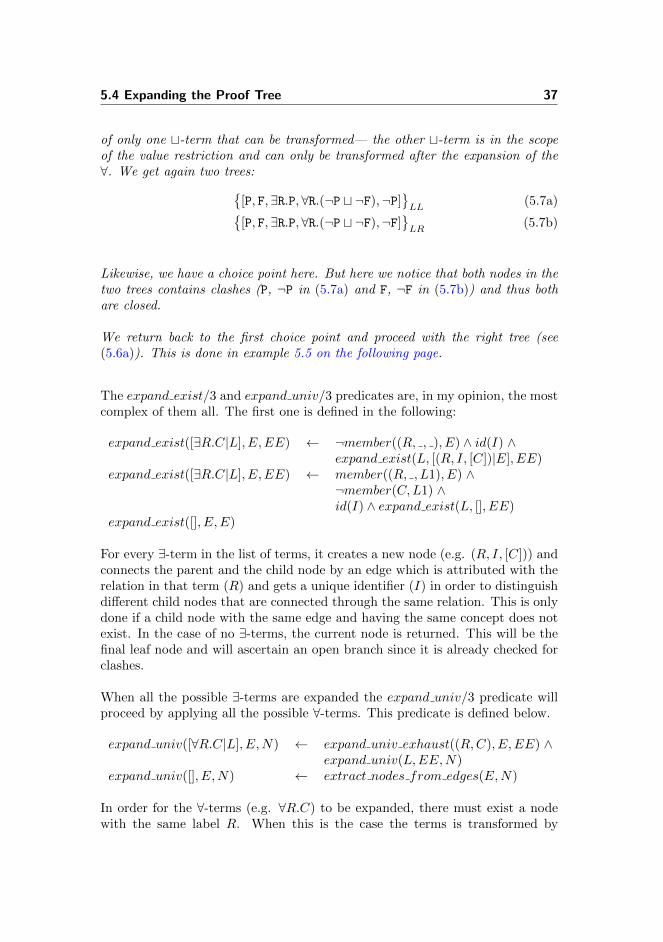
The expand exist/3 and expand univ/3 predicates are, in my opinion, the mostcomplex of them all. The first one is defined in the following:
expand exist([∃R.C|L], E,EE) ← ¬member((R, , ), E) ∧ id(I) ∧expand exist(L, [(R, I, [C])|E], EE)
expand exist([∃R.C|L], E,EE) ← member((R, , L1), E) ∧¬member(C,L1) ∧id(I) ∧ expand exist(L, [], EE)
expand exist([], E,E)
For every ∃-term in the list of terms, it creates a new node (e.g. (R, I, [C])) andconnects the parent and the child node by an edge which is attributed with therelation in that term (R) and gets a unique identifier (I) in order to distinguishdifferent child nodes that are connected through the same relation. This is onlydone if a child node with the same edge and having the same concept does notexist. In the case of no ∃-terms, the current node is returned. This will be thefinal leaf node and will ascertain an open branch since it is already checked forclashes.
When all the possible ∃-terms are expanded the expand univ/3 predicate willproceed by applying all the possible ∀-terms. This predicate is defined below.
expand univ([∀R.C|L], E,N) ← expand univ exhaust((R,C), E,EE) ∧expand univ(L,EE,N)
expand univ([], E,N) ← extract nodes from edges(E,N)
In order for the ∀-terms (e.g. ∀R.C) to be expanded, there must exist a nodewith the same label R. When this is the case the terms is transformed by

38 Specification of the Implemented Tableaux
adding the concept C to the node. The predicate, expand univ/3, does thisusing a helper predicate, expand univ exhaust/3, which applies the given ∀-term exhaustively to the list of child nodes [2, p. 38]. This predicate is definedbelow.
expand univ exhaust((R,C), E,E) ←extract((R, I, L1), E,E1) ∧ ¬member() ∧expand univ exhaust((R,C), [(R, I, [C|L1])|E1], EE)
expand univ exhaust( , E,E)
The expand predicate/3 predicate, unlike, the expand exist/3 returns the listof the child nodes without attributes when every ∀-term has been exhaustivelyapplied to the list of child nodes. This is clarified in example 5.5. Moreover,this examples gives a very clear picture of how the two predicates operate.
Example 5.5 This example is the last example in the series of examples illus-trating the specification of the tableaux.pl. In this example we proceed with theright tree, (5.6a), from example 5.4 on page 36.
This tree consists of a single node which does not have any u/t-connectives thatcan be eliminated. We, therefore, start with the expansion of the quantifiers. Theresult is: {
[P, F,∀R.(¬P t ¬F),∀R.(¬P)], [(R, 1, [P])]}
The ∃-term, ∃R.P, is pruned from the parent node and a new child node, (R, 1, [P]),attributed with R is instead created. Now, if possible, the ∀-terms are expanded.
It seems that both ∀-terms can be expanded since they scope over the same re-lation as the ∃-term expanded above, i.e. the relation R is shared by both terms.The two terms are pruned from the parent node and their concepts are added tothe child node. The result is then as shown below.{
[P, F], [(R, 1, [(¬P t ¬F),¬P, P])]}
Now the parent node, [P, F], is discarded, since it does not contribute any moreto the proof procedure. The proof procedure proceeds with the new node instead(without the attributes). This node is{
[(¬P t ¬F),¬P, P]}
In this point in the proof procedure the node is transformed by eliminating theu/t-connectives. Although, there is an obvious clash in the node, it is notdiscovered until all the connectives are eliminated. In the above node we haveonly one t-connective which is eliminated. The result is{
[¬P,¬P, P]}RL{
[¬F,¬P, P]}RR

5.4 Expanding the Proof Tree 39
which gives two trees with an immediate clash in both. This closes also theright tree from the initial node. Thus, the tableaux is saturated and all treesare closed. This means that there is no model for the proof goal. The answerto (5.1) is ’Yes’, i.e. the concept of Mother is a more general concept thanMotherWithoutDaughter.

40 Specification of the Implemented Tableaux
Chapter 6
Extending the TableauxImplementation
In his conclusion, Herchenroder lists a number of possible ways to extend thetableaux implementation, tableaux.pl, put forth by him. The extensions putforth in this work are close to two of the extensions suggested by him. Since thefocus of this work is to develop resources for use in education the developmentof the extensions was also focused in this direction.
In this chapter I present the two extensions I have developed for the tableaux.pl.Moreover I will also cover testing of these extensions here.
6.1 Ontology Format Converter
In his work, Herchenroder supports a specific format for expressing ALC expres-sions in Prolog. For instance (5.4) from example 5.2 on page 33 is expressed asshown below (negation is expressed using tilde).
and(and(and(and(P, F), exist(R, P)), forall(R, ~and(P, F))),
~and(and(P, F), exist(R, P)))

42 Extending the Tableaux Implementation
As one can see, this format is very difficult for humans to read. Moreover it isvery easy to make mistakes when constructing complex expressions. In order tomake this format more human-friendly, I have developed another format and aconverter that can convert an expression between the two formats. For instanceexpressing the above expression in this format we will get:
((P /\ F) /\ R?P /\ R!(~(P /\ F))) /\ ~((P /\ F) /\ R?P)
where tilde still expresses negation, the forward- and backslash (/\) expressesconjunction, the question mark (?) expresses existential restriction, while ex-clamation mark (!) expresses value restriction. The operator that is missingin above expression is disjunction. This operator is expressed by a back- andforwardslash (\/).
In the following section the specification of this format is given. Moreover theOntology Format Converter (OFC) that is developed to covert between the twoformats is also specified and described.
6.1.1 Specification
The ontology format which is developed by Herchenroder (from now on internalformat) enables one to express also axioms and hypotheses (queries) and notonly concept description. The ontology format which is developed by me (fromnow on external format) only supports expressing of concept description, i.e.concepts that are constructed using negation, union, intersection, existentialand value restriction or the combination of these.
The external format is very close to the syntax of the ALC. For instance theexpression A uB is just expressed as it is, just by changing the operator to /\.Expressing the quantifier, however, differs a big deal. These are actually alsoimplemented as binary operators. The normal term ∃R.C is expressed as R?Cwhere the left side of the ? is the role and the right side is the concept. Likewise,the value restriction is implemented as binary operator. For instance the term∀R.C is expressed as R!C.
In order to remember that exclamation mark is the symbol for value restrictionand question mark is the symbol for existential restriction in this format, onecan think of existential quantifier as a question, i.e. is there exist a x suchthat . . . .

6.1 Ontology Format Converter 43
A predicate, symbol operator/2, is used in order to map the operators in theinternal and external formats. This predicate is defined as presented below.
symbol operator(!, forall)symbol operator(?, exist)symbol operator(\/, or)symbol operator(/\, and)symbol operator(∼,∼)
In addition to this predicate, there are two more predicates which convertsan expression in internal format to the equal expression in external format andvise versa. These predicates are to external/2 and to internal/2. As the namessuggest, the to external/2 predicate takes an expression in internal format andreturns it in external format. Likewise, the to internal/2 predicate takes anexpression in external format an returns it in internal format.
The to external/2 predicate consists of three clauses. These are defined in thefollowing.
to external(Int, Ext) ←Int =.. [Opr,X1, X2] ∧symbol operator(Sym,Opr) ∧to external(X1, Y 1) ∧to external(X2, Y 2) ∧Ext =.. [Sym, Y 1, Y 2]
to external(Int, Ext) ←Int =.. [Opr,X] ∧symbol operator(Sym,Opr) ∧to external(X,Y ) ∧Ext =.. [Sym, Y ]
to external(X,X)
The two of the three clauses each convert binary and unary operators. Thethird claus is the basis case, i.e. returns the atomic concept. Looking at the firstclaus, one can see that it converts binary operators. The Int =.. [Opr,X1, X2]term extracts the operator (Opr) and operands (X1 and X2) of an expression.The corresponding operator in external format is mapped to this operator usingthe symbol operator/2 predicate. Recursively, the operands are converted tothe external format and the expression is constructed using the term Ext =.. [Sym, Y 1, Y 2]. The second claus works in the same way as the first one, butonly converting the unary operators.
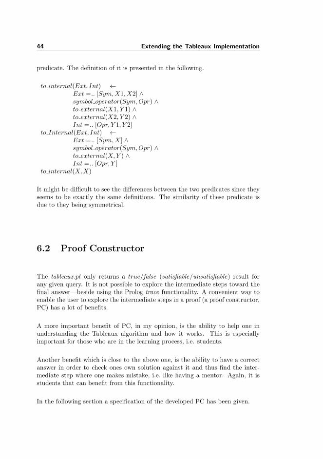
For converting from external format to internal format the predicate, to internal/2,is used. This predicate is defined exactly the same way as the to external/2
44 Extending the Tableaux Implementation
predicate. The definition of it is presented in the following.
to internal(Ext, Int) ←Ext =.. [Sym,X1, X2] ∧symbol operator(Sym,Opr) ∧to external(X1, Y 1) ∧to external(X2, Y 2) ∧Int =.. [Opr, Y 1, Y 2]
to Internal(Ext, Int) ←Ext =.. [Sym,X] ∧symbol operator(Sym,Opr) ∧to external(X,Y ) ∧Int =.. [Opr, Y ]
to internal(X,X)
It might be difficult to see the differences between the two predicates since theyseems to be exactly the same definitions. The similarity of these predicate isdue to they being symmetrical.
6.2 Proof Constructor
The tableaux.pl only returns a true/false (satisfiable/unsatisfiable) result forany given query. It is not possible to explore the intermediate steps toward thefinal answer—beside using the Prolog trace functionality. A convenient way toenable the user to explore the intermediate steps in a proof (a proof constructor,PC) has a lot of benefits.
A more important benefit of PC, in my opinion, is the ability to help one inunderstanding the Tableaux algorithm and how it works. This is especiallyimportant for those who are in the learning process, i.e. students.
Another benefit which is close to the above one, is the ability to have a correctanswer in order to check ones own solution against it and thus find the inter-mediate step where one makes mistake, i.e. like having a mentor. Again, it isstudents that can benefit from this functionality.
In the following section a specification of the developed PC has been given.

6.2 Proof Constructor 45
6.2.1 Specification
The basic idea behind the development of the PC was to take the tableaux.plas the starting point and output the result of some intermediate steps thattogether constructed the proof. It turned out that this idea could be easilyrealised and resulted in Xtableaux.pl—the extended tableaux implementation.In the following I give a specification of this extended version.
The challenges in developing the Xtableaux.pl were to output the constructedproof in a convenient way and find those intermediate steps that could result in amore constructive proof. The first challenge was easily overcome by outputtingthe constructed proof to a file. For each constructed proof the Xtableaux.pl cre-ates a file named proofX where X is a an auto-generated number distinguishingthe proofs.
To overcome the second challenge the tableaux.pl was thoroughly examined andunderstood. The intermediate steps that resulted in a more constructive proofwere chosen to be those presented in the following.
Initial Expression The expression given to the system as the hypothesis.
The Goal The reduction of the initial expression to satisfiability/unsatisfaibility,i.e. for instance the reduction of C v D to C u ¬D.
Expanded Expression The unfolding of all the name concepts, i.e. TBox-elimination.
Negative Normal Form The result of putting the expanded expression innegative normal form, i.e. pushing all the negation in the expanded ex-pression inwards until only atomic concepts are negated.
Tableaux Inference Rules The results of applying tableaux inference rulesto the initial node label in the proof tree. These results are further dividedinto intermediate steps which are as follows.
u/t-elimination The result of eliminating all possible u/t-connectivesin a node label.
∃-elimination The result of expanding all the existential restrictions ina node label.
∀-elimination The result of expanding all possible value restrictions ina node label.
Final Result The result of the proof, i.e. whether the goal is satisfiable orunsatisfiable.

46 Extending the Tableaux Implementation
The above steps means some changes to some of the predicates in tableaux.pl.These changes are highlighted in Appendix B where the complete listing ofXtableaux.pl is also given.
6.3 Testing the Extensions
In order to ensure that the correctness of the tableaux.pl is intact after theimplementation of Xtableaux.pl and the ontology format converter works asintended, some tests needed to be conducted. To this end, I have constructedtwo different test suites.
These two test suites follow the same structure. They consists of a driver pro-gram, the data sets and the programs to be tested. In the following each of thetwo test suites are described in more details.
6.3.1 Testing Ontology Format Converter
The first test suite that I will describe in this section is intended to test thecorrectness of the ontology format converter, grammar.pl.
The structure of this test suite can be summarized as follows:
grammar.pl The implementation of the ontology format converter.
ofc tester.pl The driver program that runs automatically all the test cases.
data The test cases for this test suite.
6.3.1.1 Construction of Test Data
One of the most important elements in testing any kind of software is the con-struction of test data. A constructive test data will help in revealing more bugs.It is always better that test data has been constructed by someone else then theone that has developed the software.
For this test suite, the test data has been partly taken from the ExtendedMindswap Test in Herchenroder’s work [2, p. 69] and partly has been constructedby myself.

6.3 Testing the Extensions 47
The test data that has been constructed by myself, covers the very basic casessuch as terms consisting of only one u/t-connectives. This way, the very basicbugs are revealed.
Normally, the test data consists of two parts. One part is the actual data tobe fed to the software and the other part is the expected result. The test dataconstructed for this test suite only consists of one part—there is no data partfor the expected result. This is due to the test data being used both as theactual and expected result. This is clarified further in the following section.
6.3.1.2 Conducting the Test
The way this test is conducted is not the same as the usual way—comparing theactual result of the test to the expected result. For this test suite the test datais only in the internal format which is converted to the external format usingthe to external/2 predicate. The result is used as input to the to internal/2predicate which converts the data back to the internal format—its original form.If this goes well the test is passed. This way both predicates are tested usingthe same set of data.
The test is conducted using a driver program that takes each test case and runsit like described above.
6.3.2 Testing the Proof Constructor
The second test suite is intended to test the correctness of the proof constructor,Xtableaux.pl. This test suite, like the first one, consists of many different parts.These parts are listed below.
Xtableaux.pl The extended tableaux implementation, i.e. the proof construc-tor.
grammar.pl The implementation of the ontology format converter.
pc tester.pl The driver program that runs automatically all the test cases.
data The test cases for this test suite.
As listed above, this test suite also contains the implementation of the ontologyformat converter. It is used by the proof constructor in order to convert the

48 Extending the Tableaux Implementation
expressions in the internal format to the expressions in the external formatbefore outputting them.
6.3.2.1 Construction of Test Data
For this test suite, the entire test data has been taken from the ExtendedMindswap Test in Herchenroder’s work [2, p. 69]. Each test case consists ofa hypothesis and the expected result, i.e. whether the hypothesis is satisfiableor not. Half of the test cases are TBox free while the other half has TBox.
6.3.2.2 Conducting the Test
This test suite, like the other one, is conducted using a driver program thatruns the proof constructor against every test case and tests the actual and theexpected result. If they are the same the test is passed otherwise it is failed.The whole process is automated, i.e. both the proof constructor and the testcases are loaded by the driver program and the result of each test case is givenback.
6.3.3 Test Results
The test suite for testing the ontology format converter passed error free thefirst time. This means that there were no bugs in the program that could berevealed by this test suite.
The test suite for testing the proof constructor revealed, though, some bugs.These bugs were caused by missing negation sign (∼) in some of the predicates,e.g. negnormform/2, which resulted in wrong answers some of the times. Byfixing these bugs the test suite was passed, thus ensuring the correctness of thereasoner.
Chapter 7
Conclusions
The goal of this work was to develop educational resources for teaching Descrip-tion Logics and reasoning about them using Tableaux algorithms. The startingpoint of this work was the Master Thesis of Thomas Herchenroder [2] from theUniversity of Edinburgh.
Using Herchenroder’s work and his implementation of Tableaux algorithm forreasoning in ALC, two extensions were developed. One of these extensionsintroduces an alternative ontology format, the external format, that is morehuman-friendly compared to the one used by Herchenroder, the internal format.In addition, a converter is developed that converts expressions between the twoformats.
The second extension, Xtableaux.pl, is directly developed on top of the Prologimplementation of Herchenroder, tableaux.pl. This extension, called Proof Con-structor, is meant to construct the whole proof by outputting the intermediatesteps in the proof process to a file. The intention behind this extension is tohelp students understand the Tableaux algorithms and help in debugging theontology.

50 Conclusions
7.1 Future Work
In his conclusion, Herchenroder mentions nine different ways to extend his work[2, p. 56-59]. This work, in addition to those extensions, can also be extended.
The ontology format converter can be extended with an interface that given aterm in internal format or external format outputs the result to some medium,e.g. a file.
It is also possible to extend the proof constructor. One way would be to outputthe constructed proof as a graphical proof tree instead of pure text.
7.2 Reflection
Looking back at the past five months, I realize that working on this project haseffected me in many levels. One important thing which I have learned in thecourse of this project was the ability to work independently. Moreover, I learnedhow to manage this kind of project – development based on reverse engineering.
Another important aspect of this project was learning more about Prolog andartificial intelligence in general. This had a profound effect on my choice ofcareer.

Appendix A
Listing of tableaux.pl
This is the code for tableaux.pl, the Tableaux reasoner that was developed byHerchenroder . The listing below is the exact copy from his work.
% tableaux.pl -- tableaux reasoner for description logics
:- use_module(library(lists)).
:- op(100,fy,~).
:- dynamic ont/1.
:- dynamic id/1.
% Main Proof Goal
tableaux_proof(Exp) :- % true/fals = satisfiable/unsatisfiable
proof(Exp).
%construct_goal
proof(equiv(A,B)) :-
\+ tabl(and(A,~B)),
\+ tabl(and(B,~A)).
proof(subsum(A,B)) :-
\+ tabl(and(A,~B)).
proof(disjoint(A,B)) :-
\+ tabl(and(A,B)).

52 Appendix A
proof(unsat(A)) :- % unsatisfiable A
\+ tabl(A).
proof(A) :- % try to satisfy everything else
tabl(A).
% main worker
tabl(Exp) :-
expand_defs(Exp,Exp1), % expand expression into most basic
negnormform(Exp1,Exp2), % NNF transformation
setID(0),
!,
search([[Exp2]],df,_). % do the proof as an agenda search
negnormform(~ ~X,X1) :-
negnormform(X,X1).
negnormform(~forall(R,C),exist(R,C1)) :-
negnormform(~C,C1).
negnormform(forall(R,C),forall(R,C1)) :-
negnormform(C,C1).
negnormform(~exist(R,C),forall(R,C1)) :-
negnormform(~C,C1).
negnormform(exist(R,C),exist(R,C1)) :-
negnormform(C,C1).
negnormform(~and(A,B),or(A1,B1)) :-
negnormform(~A,A1),
negnormform(~B,B1).
negnormform(and(A,B),and(A1,B1)) :-
negnormform(A,A1),
negnormform(B,B1).
negnormform(~or(A,B),and(A1,B1)) :-
negnormform(~A,A1),
negnormform(~B,B1).
negnormform(or(A,B),or(A1,B1)) :-
negnormform(A,A1),
negnormform(B,B1).
negnormform(~X,~X) :-
atom(X).
negnormform(X,X) :-
atom(X).
expand_defs(forall(R,C),forall(R,C1)) :-
expand_defs(C,C1).
expand_defs(exist(R,C),exist(R,C1)) :-
expand_defs(C,C1).
expand_defs(and(A,B),and(A1,B1)) :-

Listing of tableaux.pl 53
expand_defs(A,A1),
expand_defs(B,B1).
expand_defs(or(A,B),or(A1,B1)) :-
expand_defs(A,A1),
expand_defs(B,B1).
expand_defs(~A,~A1) :-
expand_defs(A,A1).
expand_defs(X,Y) :-
atom(X),
ont(equiv(X,X1)),
expand_defs(X1,Y).
expand_defs(X,X) :-
atom(X),
\+ ont(equiv(X,_)).
% search(+Goal,+Style,-ResultList) -- agenda style search
% -- transforms Goal into a list of [clash]/[model] elements
search([],_,[]).
search(Reduced, _, Reduced) :-
Reduced = [H|_],
H = [clash], % a clash leaf fails the proof
!,
fail.
search([Node| T], Style, Reduced) :-
process_node(Node,NewNodes),
filter_nodes(NewNodes,NewNodes1),
merge_agendas(NewNodes1, T, Style, New),
search(New, Style, Reduced).
filter_nodes(NewNodes,NewNodes1) :-
( setof(X,(member(X,NewNodes),X\=[model]),NewNodes1);
NewNodes1 = []),
!.
merge_agendas(A1, A2, df, New) :-
append(A1, A2, New),!.
merge_agendas(A1, A2, bf, New) :-
append(A2, A1, New),!.
% reduce a node of the proof tree
process_node([clash],[]) :- !.
process_node([model],[]) :- !.
process_node(ListOfDLExps,ResultListOfLists) :-
transform_connect(ListOfDLExps,_,LoL3),
expand_nodes(LoL3,ResultListOfLists).

54 Appendix A
expand_nodes([],[]).
expand_nodes([H|R],RLoL) :-
expand_node(H,RLoL1),
expand_nodes(R,RLoL2),
append(RLoL1,RLoL2,RLoL).
% process a single node
expand_node([],[]).
expand_node([model],[[model]]) :-!.
expand_node([clash],[[clash]]) :-!.
expand_node(Node,[N1]) :-
check_clash(Node,N1),!. % clash closes this branch
expand_node(Node,N1) :-
expand_exist(Node,[],LoE), % expand existential restrictions
LoE \= [], % only continue with non-empty edges
expand_forall(Node,LoE,LoE2), % try eliminate value restrictions
extract_nodes(LoE2,N1). % get the list of new fringe nodes
expand_node(Node,[N1]) :- % model closes this branch
expand_exist(Node,[],LoE),
LoE = [],
N1 = [model].
% extract list of nodes from list of edges
extract_nodes([],[]).
extract_nodes([edge(_,_,N)|R],[N|R1]) :-
extract_nodes(R,R1).
% transform and/or connectives
transform_connect([],_,[[]]).
transform_connect([and(A,B)|R],N,R1) :-
( member(A,R) ->
( member(B,R) ->
transform_connect(R,N,R1);
transform_connect([B|R],N,R1));
( member(B,R) ->
transform_connect([A|R],N,R1);
transform_connect([A,B|R],N,R1))).
transform_connect([or(A,B)|R],N,LoL) :-
( \+ (member(A,R) ; member(B,R)) ->
( transform_connect([A|R],N,LoL);
transform_connect([B|R],N,LoL));
transform_connect(R,N,LoL)).
transform_connect([H|R],N,LoL) :-

Listing of tableaux.pl 55
H \= and(_,_),
H \= or(_,_),
transform_connect(R,N,LL1),
LL1 = [LL2],
LoL = [[H|LL2]].
% transform forall/exist quantifiers
expand_exist([],L,L).
expand_exist([exist(R,C)|T],T1,L) :-
( (member(edge(R,_,X),T1), member(C,X) ) -> % existing R edge
expand_exist(T,T1,L);
getID(Id),
expand_exist(T,[edge(R,Id,[C])|T1],L)
).
expand_exist([H|T],T1,L) :-
H \= exist(_,_),
expand_exist(T,T1,L).
expand_forall(_,[],[]).
% push concept into exist. node
expand_forall(Node,[edge(R,I,N)|RoE],[edge(R,I,N2)|R1]) :-
setof(X,member(forall(R,X), Node),C1),
append(C1,N,N1),
remove_duplicates(N1,N2),
expand_forall(Node,RoE,R1).
expand_forall(Node,[edge(R,I,N)|RoE],[edge(R,I,N)|LoE]) :-
\+ member(forall(R,_),Node),
expand_forall(Node,RoE,LoE).
check_clash(Exp,Exp1) :-
member(A,Exp),
member(~A,Exp),
Exp1 = [clash].
remove_duplicates([],[]).
remove_duplicates([H|T],[H|R]) :-
r_d(H,T,[],R1),
remove_duplicates(R1,R),!.
r_d(_,[],T,T).
r_d(E,[E|T],TT,T1) :- r_d(E,T,TT,T1).
r_d(E,[X|T],TT,T1) :- X \= E, r_d(E,T,[X|TT],T1).
getID(I):-
id(I1),

56 Appendix A
I is I1 + 1,
retract(id(I1)),
asserta(id(I)),!.
getID(I):-
\+ id(_),
I is 0,
asserta(id(I)),!.
setID(X):-
( id(Y) ->
retract(id(Y));
true
),
asserta(id(X)).

Appendix B
Listing of Xtableaux.pl
This is the Prolog code for Xtableaux.pl that extends tableaux.pl with the notionof proof construction.
% Xtableaux.pl -- The extended tableaux reasoner for description logics
:- use_module(library(lists)).
:- op(100,fy,~).
:- dynamic ont/1.
:- dynamic id/1.
:- dynamic fid/1.
:- ensure_loaded(’grammar.pl’).
% Unique file name generator
getFileID(I):-
fid(I1),
I is I1 + 1,
retract(fid(I1)),
asserta(fid(I)),!.
getFileID(I):-
\+ fid(_),
I is 0,

58 Appendix B
asserta(fid(I)),!.
getFileName(X,N) :-
getFileID(I),
atom_concat(X, I, N).
% Main Proof Goal
tableaux_proof(Exp) :- % true/false = satisfiable/unsatisfiable
getFileName(proof,F),
telling(Old),
tell(F),
write(’--- INITIAL EXPRESSION: ---’), nl,
to_ext(Exp,Fml),
write(Fml), nl,
( proof(Exp) ->
write(’- SATISFIABLE -’)
;
write(’- UNSATISFIABLE -’)
),
nl,
told,
tell(Old).
%construct_goal
proof(equiv(A,B)) :-
write(’--- GOAL: ---’), nl,
to_ext(and(A,~B),Fml1),
write(Fml1),
write(’ AND ’),
to_ext(and(B,~A),Fml2),
write(Fml2),
nl,
\+ tabl(and(A,~B)),
\+ tabl(and(B,~A)).
proof(subsum(A,B)) :-
write(’--- GOAL: ---’), nl,
to_ext(and(A,~B),Fml),
write(Fml),
nl,
\+ tabl(and(A,~B)).
proof(disjoint(A,B)) :-
write(’--- GOAL: ---’), nl,
to_ext(and(A,~B),Fml),
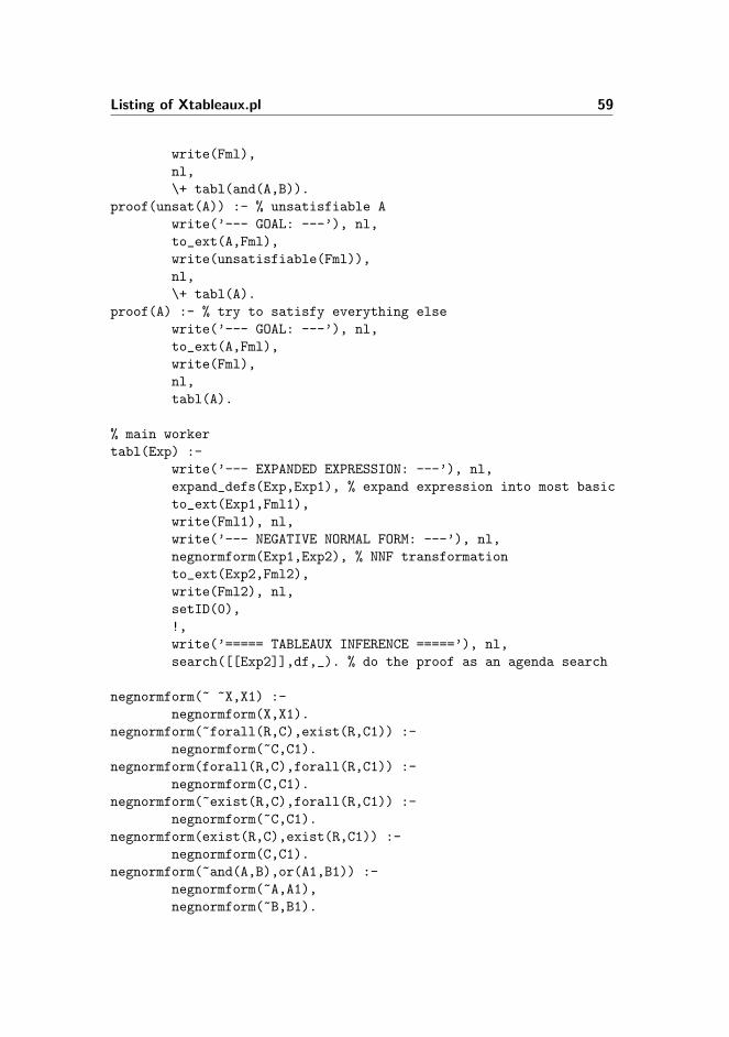
Listing of Xtableaux.pl 59
write(Fml),
nl,
\+ tabl(and(A,B)).
proof(unsat(A)) :- % unsatisfiable A
write(’--- GOAL: ---’), nl,
to_ext(A,Fml),
write(unsatisfiable(Fml)),
nl,
\+ tabl(A).
proof(A) :- % try to satisfy everything else
write(’--- GOAL: ---’), nl,
to_ext(A,Fml),
write(Fml),
nl,
tabl(A).
% main worker
tabl(Exp) :-
write(’--- EXPANDED EXPRESSION: ---’), nl,
expand_defs(Exp,Exp1), % expand expression into most basic
to_ext(Exp1,Fml1),
write(Fml1), nl,
write(’--- NEGATIVE NORMAL FORM: ---’), nl,
negnormform(Exp1,Exp2), % NNF transformation
to_ext(Exp2,Fml2),
write(Fml2), nl,
setID(0),
!,
write(’===== TABLEAUX INFERENCE =====’), nl,
search([[Exp2]],df,_). % do the proof as an agenda search
negnormform(~ ~X,X1) :-
negnormform(X,X1).
negnormform(~forall(R,C),exist(R,C1)) :-
negnormform(~C,C1).
negnormform(forall(R,C),forall(R,C1)) :-
negnormform(C,C1).
negnormform(~exist(R,C),forall(R,C1)) :-
negnormform(~C,C1).
negnormform(exist(R,C),exist(R,C1)) :-
negnormform(C,C1).
negnormform(~and(A,B),or(A1,B1)) :-
negnormform(~A,A1),
negnormform(~B,B1).
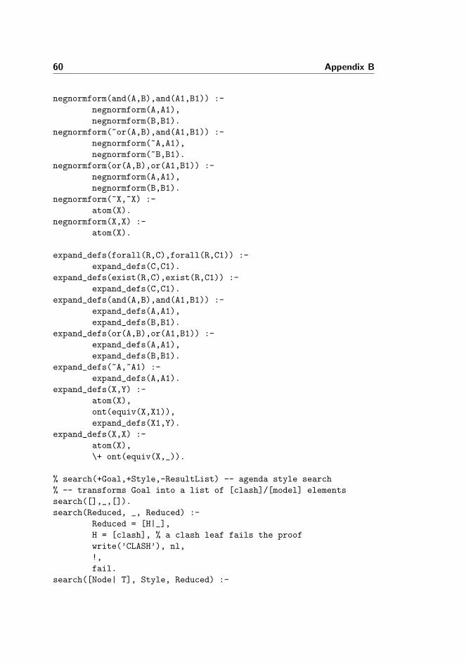
60 Appendix B
negnormform(and(A,B),and(A1,B1)) :-
negnormform(A,A1),
negnormform(B,B1).
negnormform(~or(A,B),and(A1,B1)) :-
negnormform(~A,A1),
negnormform(~B,B1).
negnormform(or(A,B),or(A1,B1)) :-
negnormform(A,A1),
negnormform(B,B1).
negnormform(~X,~X) :-
atom(X).
negnormform(X,X) :-
atom(X).
expand_defs(forall(R,C),forall(R,C1)) :-
expand_defs(C,C1).
expand_defs(exist(R,C),exist(R,C1)) :-
expand_defs(C,C1).
expand_defs(and(A,B),and(A1,B1)) :-
expand_defs(A,A1),
expand_defs(B,B1).
expand_defs(or(A,B),or(A1,B1)) :-
expand_defs(A,A1),
expand_defs(B,B1).
expand_defs(~A,~A1) :-
expand_defs(A,A1).
expand_defs(X,Y) :-
atom(X),
ont(equiv(X,X1)),
expand_defs(X1,Y).
expand_defs(X,X) :-
atom(X),
\+ ont(equiv(X,_)).
% search(+Goal,+Style,-ResultList) -- agenda style search
% -- transforms Goal into a list of [clash]/[model] elements
search([],_,[]).
search(Reduced, _, Reduced) :-
Reduced = [H|_],
H = [clash], % a clash leaf fails the proof
write(’CLASH’), nl,
!,
fail.
search([Node| T], Style, Reduced) :-
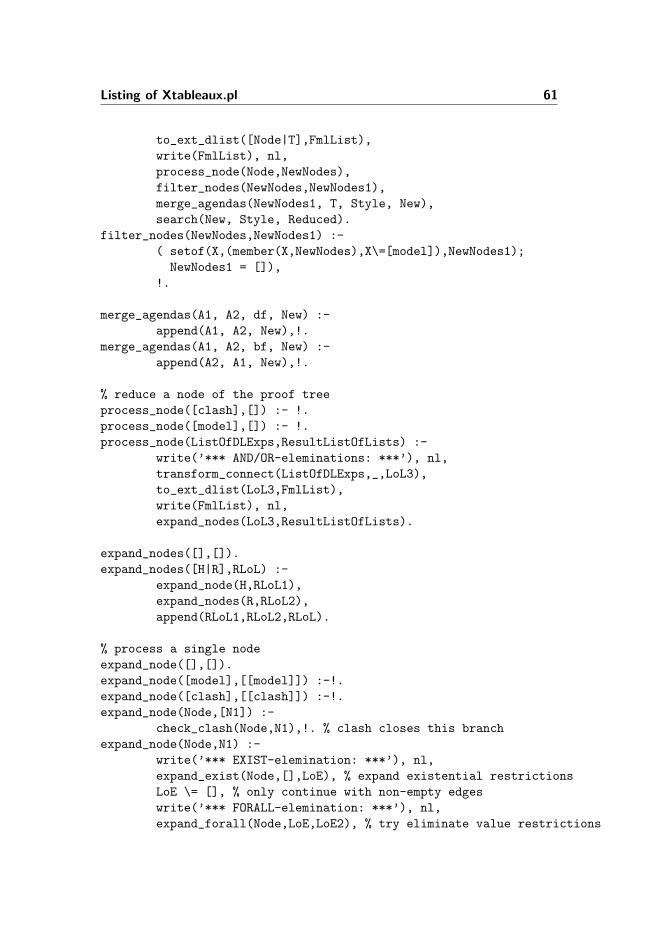
Listing of Xtableaux.pl 61
to_ext_dlist([Node|T],FmlList),
write(FmlList), nl,
process_node(Node,NewNodes),
filter_nodes(NewNodes,NewNodes1),
merge_agendas(NewNodes1, T, Style, New),
search(New, Style, Reduced).
filter_nodes(NewNodes,NewNodes1) :-
( setof(X,(member(X,NewNodes),X\=[model]),NewNodes1);
NewNodes1 = []),
!.
merge_agendas(A1, A2, df, New) :-
append(A1, A2, New),!.
merge_agendas(A1, A2, bf, New) :-
append(A2, A1, New),!.
% reduce a node of the proof tree
process_node([clash],[]) :- !.
process_node([model],[]) :- !.
process_node(ListOfDLExps,ResultListOfLists) :-
write(’*** AND/OR-eleminations: ***’), nl,
transform_connect(ListOfDLExps,_,LoL3),
to_ext_dlist(LoL3,FmlList),
write(FmlList), nl,
expand_nodes(LoL3,ResultListOfLists).
expand_nodes([],[]).
expand_nodes([H|R],RLoL) :-
expand_node(H,RLoL1),
expand_nodes(R,RLoL2),
append(RLoL1,RLoL2,RLoL).
% process a single node
expand_node([],[]).
expand_node([model],[[model]]) :-!.
expand_node([clash],[[clash]]) :-!.
expand_node(Node,[N1]) :-
check_clash(Node,N1),!. % clash closes this branch
expand_node(Node,N1) :-
write(’*** EXIST-elemination: ***’), nl,
expand_exist(Node,[],LoE), % expand existential restrictions
LoE \= [], % only continue with non-empty edges
write(’*** FORALL-elemination: ***’), nl,
expand_forall(Node,LoE,LoE2), % try eliminate value restrictions

62 Appendix B
extract_nodes(LoE2,N1), % get the list of new fringe nodes
write(’*** NEW FRINGE NODES: ***’), nl,
!. %%% ADDED by ISMAIL (closes this branch)
expand_node(Node,[N1]) :- % model closes this branch
expand_exist(Node,[],LoE),
LoE = [],
N1 = [model].
% extract list of nodes from list of edges
extract_nodes([],[]).
extract_nodes([edge(_,_,N)|R],[N|R1]) :-
extract_nodes(R,R1).
% transform and/or connectives
transform_connect([],_,[[]]).
transform_connect([and(A,B)|R],N,R1) :-
( member(A,R) ->
( member(B,R) ->
transform_connect(R,N,R1);
transform_connect([B|R],N,R1));
( member(B,R) ->
transform_connect([A|R],N,R1);
transform_connect([A,B|R],N,R1))).
transform_connect([or(A,B)|R],N,LoL) :-
( \+ (member(A,R) ; member(B,R)) ->
( transform_connect([A|R],N,LoL);
transform_connect([B|R],N,LoL));
transform_connect(R,N,LoL)).
transform_connect([H|R],N,LoL) :-
H \= and(_,_),
H \= or(_,_),
transform_connect(R,N,LL1),
LL1 = [LL2],
LoL = [[H|LL2]].
% transform forall/exist quantifiers
expand_exist([],L,L).
expand_exist([exist(R,C)|T],T1,L) :-
( (member(edge(R,_,X),T1), member(C,X) ) -> % existing R edge
expand_exist(T,T1,L);
getID(Id),
write(’ ’),
to_ext(C,Fml),
write([edge(R,Id,[Fml])]),

Listing of Xtableaux.pl 63
nl,
expand_exist(T,[edge(R,Id,[C])|T1],L)
).
expand_exist([H|T],T1,L) :-
H \= exist(_,_),
expand_exist(T,T1,L).
expand_forall(_,[],[]).
% push concept into exist. node
expand_forall(Node,[edge(R,I,N)|RoE],[edge(R,I,N2)|R1]) :-
setof(X,member(forall(R,X), Node),C1),
append(C1,N,N1),
remove_duplicates(N1,N2),
write(’ ’),
to_ext_list(N2,Fml),
write([edge(R,I,Fml)]),
nl,
expand_forall(Node,RoE,R1).
expand_forall(Node,[edge(R,I,N)|RoE],[edge(R,I,N)|LoE]) :-
\+ member(forall(R,_),Node),
expand_forall(Node,RoE,LoE).
check_clash(Exp,Exp1) :-
member(A,Exp),
member(~A,Exp),
Exp1 = [clash].
remove_duplicates([],[]).
remove_duplicates([H|T],[H|R]) :-
r_d(H,T,[],R1),
remove_duplicates(R1,R),!.
r_d(_,[],T,T).
r_d(E,[E|T],TT,T1) :- r_d(E,T,TT,T1).
r_d(E,[X|T],TT,T1) :- X \= E, r_d(E,T,[X|TT],T1).
getID(I):-
id(I1),
I is I1 + 1,
retract(id(I1)),
asserta(id(I)),!.
getID(I):-
\+ id(_),
I is 0,
asserta(id(I)),!.
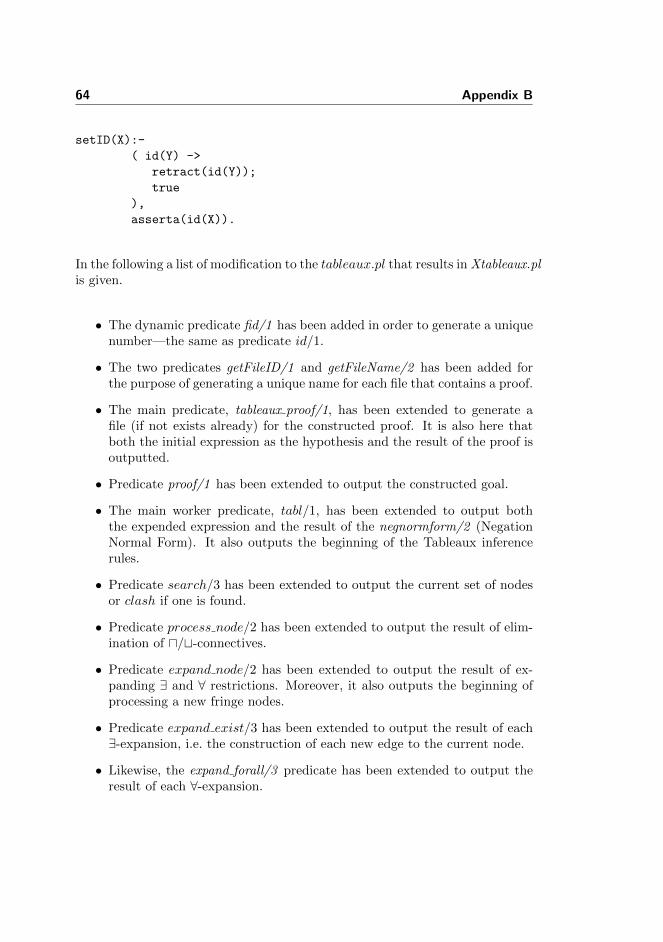
64 Appendix B
setID(X):-
( id(Y) ->
retract(id(Y));
true
),
asserta(id(X)).
In the following a list of modification to the tableaux.pl that results in Xtableaux.plis given.
• The dynamic predicate fid/1 has been added in order to generate a uniquenumber—the same as predicate id/1.
• The two predicates getFileID/1 and getFileName/2 has been added forthe purpose of generating a unique name for each file that contains a proof.
• The main predicate, tableaux proof/1, has been extended to generate afile (if not exists already) for the constructed proof. It is also here thatboth the initial expression as the hypothesis and the result of the proof isoutputted.
• Predicate proof/1 has been extended to output the constructed goal.
• The main worker predicate, tabl/1, has been extended to output boththe expended expression and the result of the negnormform/2 (NegationNormal Form). It also outputs the beginning of the Tableaux inferencerules.
• Predicate search/3 has been extended to output the current set of nodesor clash if one is found.
• Predicate process node/2 has been extended to output the result of elim-ination of u/t-connectives.
• Predicate expand node/2 has been extended to output the result of ex-panding ∃ and ∀ restrictions. Moreover, it also outputs the beginning ofprocessing a new fringe nodes.
• Predicate expand exist/3 has been extended to output the result of each∃-expansion, i.e. the construction of each new edge to the current node.
• Likewise, the expand forall/3 predicate has been extended to output theresult of each ∀-expansion.
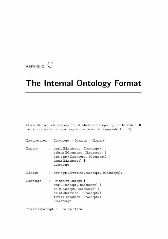
Appendix C
The Internal Ontology Format
This is the complete ontology format which is developed by Herchenroder . Ithas been presented the same way as it is presented in appendix D in [2].
DLexpression :: DLconcept | DLaxiom | DLquery
DLquery :: equiv(DLconcept, DLconcept) |
subsum(DLconcept, DLconcept) |
disjoint(DLconcept, DLconcept) |
unsat(DLconcept) |
DLconcept
DLaxiom :: ont(equiv(PrimitiveConcept, DLconcept))
DLconcept :: PrimitiveConcept |
and(DLconcept, DLconcept) |
or(DLconcept, DLconcept) |
exist(Relation, DLconcept)|
forall(Relation,DLconcept)|
~DLconcept
PrimitiveConcept :: PrologLiteral
66 Appendix C
Relation :: PrologLiteral

Appendix D
Listing of grammar.pl
This is the Prolog code for the grammar.pl—the ontology format converter.
:- op(650,xfy,!). /* universal */
:- op(640,xfy,?). /* existential */
:- op(630,xfy,\/). /* disjunction */
:- op(620,xfy,/\). /* conjunction */
:- op(610,fy,~). /* negation */
sym_opr(!,forall).
sym_opr(?,exist).
sym_opr(\/,or).
sym_opr(/\,and).
sym_opr(~,~).
%
% Convert to Externel Format
%
to_ext(Int, Ext) :-
Int =.. [Opr, X1, X2],
sym_opr(Sym, Opr), !,
to_ext(X1, Y1),

68 Appendix D
to_ext(X2, Y2),
Ext =.. [Sym, Y1, Y2].
to_ext(Int, Ext) :-
Int =.. [Opr, X1],
sym_opr(Sym, Opr), !,
to_ext(X1, Y1),
Ext =.. [Sym, Y1].
to_ext(F, F).
%
% Convert to Internal Format
%
to_int(Ext, Int) :-
Ext =.. [Sym, X1, X2],
sym_opr(Sym, Opr), !,
to_int(X1, Y1),
to_int(X2, Y2),
Int =.. [Opr, Y1, Y2].
to_int(Ext, Int) :-
Ext =.. [Sym, X1],
sym_opr(Sym, Opr), !,
to_int(X1, Y1),
Int =.. [Opr, Y1].
to_int(F, F).
%
% Convert a list of internal formulas to external format
%
to_ext_list([X|T],[Fml|L]):-
to_ext(X,Fml),
to_ext_list(T,L).
to_ext_list([],[]).
%
% Convert a two-diminsional list of internal formulas to external format
%
to_ext_dlist([X|T],[Y|L]) :-
to_ext_list(X,Y),
to_ext_dlist(T,L).

Listing of grammar.pl 69
to_ext_dlist([],[]).
The two predicates to ext dlist/2 and to ext list/2 has been developed in orderto process a two dimensional and one dimensional lists of nodes, respectively.They are used in the development of the proof constructor (see section 6.2 onpage 44).

70 Appendix D

Appendix E
Test Data for ProofConstructor
This is the test data used in the test suite that tested the correctness of theproof constructor. There are in total 10 files where each file name is proceededby its content.
ex1_1.pl:
sat(false).
query( and( wine, beer)).
ont(equiv(beer,and( drink,and(exist( hasingr, water),
and( exist( hasingr,hops),and( exist( hasingr, malt),
forall( hasingr, or( water, or(hops,malt))))))))).
ont(equiv(grapes,and( (~hops),and( (~malt), (~water))))).
ont(equiv(wine,and( drink, exist( hasingr, grapes)))).
ex1_2_1.pl:
sat(false).
query( and( exist( r, b), forall( r, (~b)))).
ex1_2_2.pl:
sat(true).
query( and( exist( r, b), forall( r, or( a, (~b))))).

72 Appendix E
ex1_2_3.pl:
sat(false).
query( and( exist( r, b), forall( r, (~b)))).
ont(equiv(aa,or( a, (~a)))).
ont(equiv(a,exist( r, exist( r, exist( r, c))))).
ont(equiv(b,and( a, and(exist( r, aa), or( aa, (~aa)))))).
ex1_2_4.pl:
sat(false).
query( and( exist( r, b), forall( r, or( a, (~b))))).
ont(equiv(a,( ~b))).
ex1_3.pl:
sat(true).
query( and( werewolf, human)).
ont(equiv(werewolf,and( animal, and(exist( haspower,
magical),forall( speaks, language))))).
ont(equiv(acramantula,and( beast,and(or( male,
female),exist( haspower, magical))))).
ont(equiv(wizard,and( male,and(human,exist(
haspower, magical))))).
ont(equiv(centaur,and( animal,and((~human),and(
or( male, female),and(exist(haspower, magical),
forall( speaks, language))))))).
ont(equiv(vampire,and( beast,and(or( male,
female),forall( haspower,magical))))).
ont(equiv(beast,and( animal,(~human)))).
ont(equiv(muggle,and( human,and( or( male,
female),forall( haspower,(~magical)))))).
ont(equiv(witch,and( female,and( human,
exist( haspower, magical))))).
ont(equiv(human,and( animal,exist( speaks, language)))).
ont(equiv(male,and( animal,(~female)))).
ont(equiv(merpeople,and( animal,and( (~human),
and( forall( haspower, magical),forall( speaks,
language)))))).
ex1_8.pl:
sat(true).
query( or( and( or( a, b), or( c, d)),
and( or( a, c), or( b, d)))).
ex1_10.pl:

Test Data for Proof Constructor 73
sat(true).
query( and( veggiepizza, meatpizza)).
ont(equiv(veggiepizza,and( pizza, forall( hastopping,
(~meat))))).
ont(equiv(meatpizza,and( pizza, forall( hastopping,
(~veggie))))).
ont(equiv(veggie,or( mushroom, olive))).
ont(equiv(meat,or( pepperoni, sausage))).
ex1_11.pl:
sat(false).
query( and( exist( p, a), and(exist( p, b), and(
and( c, d), (~exist( p, (~and((~e), f)))))))).
ont(equiv(a,and( h, and( i, (~d))))).
ont(equiv(j,( ~k))).
ont(equiv(b,( ~g))).
ont(equiv(d,forall( q, j))).
ont(equiv(g,( ~e))).
ex2_7.pl:
sat(true).
query( and( b, and(c, and(exist( p, and( a,
and(c, exist( r, (~d))))), forall(r, d))))).

74 Appendix E

Appendix F
Test Data for OntologyFormat Converter
This is the test data used in the test suite that tested the correctness of theontology format converter. There are in total 10 files where each file name isproceeded by its content. The 4 first files are constructed by myself. The restof the files indicate where their content come from using Prolog comments. Thefiles that are indicated in the comments are from the Extended Mindswap Tests[2, p. 69-80].
exp_1.pl:
query(and( a, b)).
exp_2.pl:
query(or( a, b)).
exp_3.pl:
query(exist(r, b)).
exp_4.pl:
query(forall(r, a)).
exp_5.pl:

76 Appendix F
%
% The query from ex1_11.pl
%
query( and( exist( p, a), and(exist( p, b),
and(and( c, d), (~exist( p, (~and((~e), f)))))))).
exp_6.pl:
%
% The query from ex1_2_1.pl
%
query( and( exist( r, b), forall( r, (~b)))).
exp_7.pl:
%
% The query from ex1_2_2.pl
%
query( and( exist( r, b), forall( r, or( a, (~b))))).
exp_8.pl:
%
% The query from ex1_8.pl
%
query( or( and( or( a, b), or( c, d)),
and( or( a, c), or( b, d)))).
exp_9.pl:
%
% The query from ex1_9.pl
%
query( and( hydra, and( dragonet, exist( elemental, fire)))).
exp_10.pl:
%
% The query from ex2_1.pl
%
query( and( a, and(d, and(g, and((~m), and((~n),
and((~o), and((~p), and((~q), and((~r),
and((~s), and((~t), and((~u), and((~v1),
and((~w),(~x)))))))))))))))).

Appendix G
Test Driver Scripts
The following two programs have been used as driver scripts for the two testsuites.
G.1 Listing of pc tester.pl
This is the code for the program that runs Xtableaux.pl against the test datapresented in appendix E on page 71. The invocation of the program looked like
swipl -s pc tester.pl -g run. -t halt.
%%%%%%%%%%%%%%%%%%%%%%%%%%%%%%%%%%%%%%%%
% pc_tester.pl %
%%%%%%%%%%%%%%%%%%%%%%%%%%%%%%%%%%%%%%%%
% Performs tests on the Xtableaux.pl
% in order to ensure the correctness of it.
% Inspired from reg_test.pl developed
% by Thomas Herschenroeder
:- consult(’Xtableaux.pl’).

78 Appendix G
% A small program to read data from a file
% and assert it to the database
%
% The program is taken from:
% http://www.csupomona.edu/~jrfisher/www/prolog_tutorial/pt_framer.html
%
% It has been slightly modified
browse(File) :-
seeing(Old),
see(File),
repeat,
read(Data),
process(Data),
seen,
see(Old),
!.
process(end_of_file) :- !.
process(Data) :- assert(Data), fail.
% dir interface
get_files(Dir):-
consult(Dir), % get list of test files
flist(Files), % into a variable
eval_files(Files).
eval_files([F|T]):-
eval_file(F),
eval_files(T).
eval_file(File1):-
retractall(query(_)),
retractall(sat(_)),
retractall(ont(_)),
atom_concat(’data/’,File1,File),
browse(File),
write(’Testing file: ’), write(File), nl,
query(Q),
sat(S),
tableaux_proof(Q,S1),
( S1 = S -> report(File,ok) ; report(File,err)).
report(File,ok):-

G.2 Listing of ofc tester.pl 79
write(File),write(’: OK’),nl.
report(File,err):-
write(File), write(’: ERROR’),nl.
% Runs the test suite
run :- get_files(’data/index.pl’).
G.2 Listing of ofc tester.pl
This is the code for the program that runs grammar.pl against the test datapresented in appendix F on page 75. The invocation of the program looked like
swipl -s ofc tester.pl -g run. -t halt.
%%%%%%%%%%%%%%%%%%%%%%%%%%%%%%%%%%%%%%%%%
% ofc_tester.pl %
%%%%%%%%%%%%%%%%%%%%%%%%%%%%%%%%%%%%%%%%%
% Runs the test data for ontology format
% converter in order to test the correctness of it.
% Inspired from reg_test.pl developed by
% Thomas Herschenroeder
:- consult(’grammar.pl’).
% A small program to read data from a file
% and assert it to the database
%
% The program is taken from:
% http://www.csupomona.edu/~jrfisher/www/prolog_tutorial/pt_framer.html
%
% It has been slightly modified
browse(File) :-
seeing(Old),
see(File),
repeat,
read(Data),
process(Data),
seen,
see(Old),
!.

80 Appendix G
process(end_of_file) :- !.
process(Data) :- assert(Data), fail.
% dir interface
get_files(Dir):-
consult(Dir), % get list of test files
flist(Files), % into a variable
eval_files(Files).
eval_files([F|T]):-
eval_file(F),
eval_files(T).
eval_file(File1):-
retractall(query(_)),
atom_concat(’data/’,File1,File),
browse(File),
write(’Testing file: ’), write(File), nl,
query(Q),
to_ext(Q,Fml), % convert to external format
( to_int(Fml,Q) -> % convert it back to internal
report(File,ok);
report(File,err)).
report(File,ok):-
write(File),write(’: OK’),nl.
report(File,err):-
write(File), write(’: ERROR’),nl.
% Runs the test suite
run :- get_files(’data/index.pl’).

Bibliography
[1] F. Baader, D. Calvanesse, D. L. McGuinness, D. Nardi and P. F. Patel-Schneider, The Description Logic Handbook : Theory, Implementation andApplication, Cambridge University Press,Second Edition, 2010.
[2] Thomas Herchenroder, Lightweight Semnatic Web Oriented Reasoning inProlog: Tableaux Inferences for Description Logics, University of Edin-burgh, 2006,
[3] D. Nardi and R. J. Brachman, An Introduction to Description Logics inThe Description Logic Handbook, Cambridge University Press,Second Edition, pp. 1–43.
[4] D. Nardi and R. J. Brachman, Basic Description Logics in The DescriptionLogic Handbook, Cambridge University Press,Second Edition, pp. 47–104.
[5] Franz Baader, Description Logics, Theoretical Computer Science, TU Dres-den, Germany, 2009, volume 5689, URL: http://lat.inf.tu-dresden.de/research/papers-2009.html#Baader09
[6] Ian Horrocks, OWL: A Description Logic Based Ontology Language, Talkat CISA, Edinburgh, March 30th 2006 URL: http://www.cs.man.ac.uk/
~horrocks/Slides/index.html