a demographic analysis of lesser prairie ...table 6. estimates for age-specific survival and...

A DEMOGRAPHIC ANALYSIS OF LESSER PRAIRIE-CHICKEN POPULATIONS IN SOUTHWESTERN KANSAS: SURVIVAL, POPULATION VIABILITY, AND

HABITAT USE

by

CHRISTIAN ANDREW HAGEN

B. A., Fort Lewis College, 1993

M.N.R.M., University of Manitoba, 1999

----------------------------------------------

A DISSERTATION

submitted in partial fulfillment of the

requirements for the degree

DOCTOR OF PHILOSOPHY

Division of Biology College of Arts and Sciences

KANSAS STATE UNIVERSITY

2003

Approved by:

Major Professor Robert J. Robel

ABSTRACT

Lesser prairie-chicken (Tympanuchus pallidicinctus) habitat and populations have

been reduced range-wide by more than 90% since the turn of 20th Century. Population

indices in Kansas reflected the range-wide trends. The rate of habitat loss slowed

considerably starting in the 1980s, but populations have continued to decline in the state.

To aid in the conservation of this “warranted but precluded” threatened species, more

information is needed on the basic and applied population ecology of this prairie grouse.

The present research was initiated to collect field data for 3-years and synthesize 6-years

of data from 2 Federal Aid projects in southwestern Kansas.

I used age-structured mark-recapture models to estimate the local survival rates of

banded yearling and adult male lesser prairie-chickens from live mark-recapture data.

Local survival rates of male lesser prairie-chickens were ranked: yearling (φ1 = 0.615, SE

= 0.068) > adult (φ1 = 0.485, SE = 0.058) > older adults (φ2 = 0.347, SE = 0.047).

Using joint models of live encounter and dead recovery, I examined the potential

for bias in survival estimates of radiomarked male lesser prairie-chickens. The model best

supported by the data, Ŝc, pgroup+t, rg, Fc, indicated that survival was best modeled as not

different (Ŝc = 0.731, SE = 0.072) across radiomarked and banded birds.

I evaluated the effects of season, age, and gender on survival of radiomarked

birds. The known-fate analysis revealed that overall male (Ŝ = 0.71, SE = 0.06) and hen

(Ŝ = 0.69, SE = 0.06) survival rates were similar, but hens were most susceptible to

mortality during nesting. Additionally, yearling females had a greater probability (Ŝ =

0.77, SE = 0.06) of surviving than adults (Ŝ = 0.62, SE = 0.05).

Population viability and management alternatives were examined using elasticity

analysis on an age-specific projection matrix. The model was parameterized with

demographic data from this field study. The rate of population change (λ) was < 1.0 for

both populations (λI = 0.544, λII = 0.754). This indicated a short-term decline in

population growth in the absence of immigration. However, the marked contrast in the

contributions to λ between populations were explained by nest success and chick

survival, and prescribed management practices should focus on these rates.

I examined the relationship of several habitat characteristics and landscape

features as they pertained to habitat suitability in southwestern Kansas. I quantified these

characteristics in use and non-use sites as determined from the presence or absence of

prairie chicken locations. Multivariate analyses indicated that site occupancy was

explained, in part, by moderate densities of sagebrush, but negatively associated with the

proximity to anthropogenic features (e.g., powerlines, roads, buildlings, and pump-jacks).

TABLE OF CONTENTS List of figures………….…………………………….…………..…………………..……iv

List of tables………………………………………..……………………………..…..…vii Acknowledgements……………………………………………….…………………..…...x Introduction………………………………………………………….…………………….1 Chapter 1: Age-specific survival of male lesser prairie-chickens…...…………………..16

Introduction…………………….....………………………………………….......17

Study Area……………………….…………………………………………........20

Field Methods……….......………..…….…………………………………….….20

Data Analysis………………………………………………..…………………...21

Results…………………………..………………………………………………..24

Discussion………………………………………..………………………………25

Literature Cited…………………………………………..……………….………31

Chapter 2: Radiotelemetry estimates of survival in the lesser prairie-chicken: are there

biases?……………………………………………………………………………45

Introduction…………………….....………………………………………….......46

Field Methods……….......………..…….…………………………………….….48

Data Analysis………………………………………………..…………………...49

Results…………………………..………………………………………………..52

Discussion………………………………………..………………………………54

Literature Cited…………………………………………..……………….………57

i

Chapter 3: Gender and age-specific survival and probable causes of mortality in

radiomarked lesser prairie-chickens in Kansas…...……………………………..65

Introduction…………………….....………………………………………….......66

Study Area……………………….…………………………………………........68

Field Methods……….......………..…….…………………………………….….69

Data Analysis………………………………………………..…………………...71

Results…………………………..………………………………………………..73

Discussion………………………………………..………………………………76

Literature Cited…………………………………………..……………….………83 Chapter 4: Lesser prairie-chicken demography: a sensitivity analysis of population

dynamics in two prairie fragments…...………………………………………...104

Introduction…………………….....………………………………………….....105

Study Area……………………….…………………………………………......108

Field Methods………......………..…….…………………………………….…109

Data Analysis………………………………………………..……………..…..110

Results…………………………..…………………………………….………..116

Discussion………………………………………..………………..…….…..…120

Literature Cited…………………………………………..……………….……128

Chapter 5: The effects of landscape features on lesser prairie-chicken habitat use……145 Introduction…………………….....………………………………………….....146

Study Area……………………….…………………………………………......147

Field Methods……….......………..…….…………………………..……….….148

Data Analysis………………………………………………..………………….149

ii

Results………………………..………………………………..……………….154

Discussion……………………………………………..…..……………………156

Literature Cited……..…………………………………..……………….………159 Overall Summary………………………………………….……………………..…….173

Appendix I: Genetic evaluation of lesser prairie-chickens….………………………….179

Appendix II: Tables of lesser prairie-chicken morphometrics.…………..…………….198

iii

LIST OF FIGURES Introduction Fig. 1. Historic and current distribution of lesser prairie-chickens in Kansas. Note extra-

limit records for several studies denoted by small symbols (see map legend for details)………………………………………………………………………………13

Fig. 2. Population trends (birds/mi2) of lesser prairie-chickens from lek survey data

(1964-2002) from 4 to10 survey routes (A). The relationship between lek survey data and available rangeland for counties where surveys were conducted (B). Five-year intervals were used because US Census of Agriculture quantified available pasture at those approximate intervals. Lek survey data were averaged across each 5-year interval to illustrate the potential long term effects of large-scale habitat loss………………………………………………………………………………….15

Chapter 1

No figures Chapter 2 Fig. 1. The cumulative frequency distribution (A) of mortalities and right-censoring

indicates that the high mortality periods (2-week intervals) were not associated with right censoring. The distribution of mortality and right-censoring (B) indicates the actual numbers lost to mortality or signal in a given 2-week period were not usually related……………………………………………………………………………….64

Chapter 3 Fig. 1. Annual variation in monthly survival rates (9-months) of hens (A) from the model

S year + month, standard errors not included for clarity. Yearling and adult hen survival rates (B) from the model S year + month. Male and hen survival (C) from the model S gender*month (1997-1999)…………………………………………………………...95

Fig. 2. Relationship between biweekly survival rates of males (dashed line) and hens

(solid line) and the cumulative frequency distribution (CFD) of incubating hens (gray). Note the inverse relationship of hen survival relative to the CFD of nests...97

Fig. 3. Monthly survival rates of males and hens (A) for 12-months (2000-2003) from the

model S gender*month. Note the variation in the timing of survival between the groups. Monthly survival rates for yearlings and adults (B) for 12-months.………….…….99

Fig. 4. Nest success (black) and hen survival (white) ± SEs for 1998-2002. Nests from

1997 were not included due to different nest marking techniques..…………….101

iv

Chapter 3 (continued) Fig. 5. Reproductive parameters of female lesser prairie-chickens (black =yearling; white

= adult) from 1998 to 2002. Note the consistency among clutch size, incubation date, and probability of (re)nesting (A, B, and D) with only slight separation in nesting success (C) between the age-classes...……………………………………103

Chapter 4 Fig. 1. Life-cycle diagram and matrix for a 2 age-class pre-breeding model of female

lesser prairie-chickens. Notations for vital rates are defined in the text.…………142 Fig. 2. Results of the life-table response experiment (LTRE) show the contribution of

each vital rate to the difference in λ between Area I (lower half of panel) and Area II (upper half of panel). This retrospective analysis determined that advantages of NEST1a and CHICK on Area II and I, respectively, had the largest contribution to population growth. Notations for vital rates are defined in the text.……………..144

Chapter 5 Fig. 1. Mean canonical variates (CAN-1 and CAN-2), SEs (in both x,y) and their

respective 95 % confidence circles for lesser prairie-chicken use, non-use and absent sites……………..………………………….….……………………………..…....166

Fig. 2. Odds ratios (95% confidence limits) for roads occurring in lesser prairie-chicken

monthly-ranges in 2000 (A), 2001 (B), and 2002 (C). The dashed line indicates odds of 1 and confidence limits intersecting this line indicate odds not different than expected by chance………………………….….……………………………..…..168

Fig. 3. Odds ratios (95% confidence limits) for powerlines occurring in lesser prairie-

chicken monthly-ranges in 2000 (A), 2001 (B), and 2002 (C). The dashed line indicates odds of 1 and confidence limits intersecting this line indicate odds not different than expected by chance………………………….….…………………..170

Fig. 4. Differences in the mean number (95% confidence limits) of wells ha-1,000 between

monthly- and non-ranges as determined from Poisson rate regression. The dashed line indicates a difference of 0 and confidence limits intersecting this line indicate a observed values did not differ from those expected by chance.…………………..172

v

Appendix I Fig. 1.Sampling locations (black dots) and counties (gray polygons) of lesser prairie-

chickens for genetic evaluations. Oklahoma and New Mexico sites are from Van den Bussche et al. (2003)..…………………………………………….………..193

Fig. 2. Frequency of 45 haplotypes (pie charts) by geographic region and sampling

sites..………………………………………………………………………..…..195 Fig. 3. Neighbor-joining tree based on Nei’s unbiased minimum distance. Note the

geographic structuring of populations reflected in Fig. 2..……………………..197 Appendix II No figures

vi

LIST OF TABLES Chapter 1 Table 1. Numbers of adult and yearling lesser prairie-chicken males captured for the first

time (F) or recaptured (R) from a previous year, and trapping efforts in Finney County, Kansas……………………………………………..……………………38

Table 2. Age-specific mark-recapture modeling for male lesser prairie-chickens in Finney

County, Kansas, 1998-2002..…………………………………………..…..……39 Table 3. Local survival rates and recapture probabilities for male lesser prairie-chickens

separating survival immediately after first capture from later transitions, Finney County, Kansas, 1998-2002.………………………………………………..……40

Table 4. The numbers of within and between year interlek movements of banded male

lesser prairie-chickens, Finney County, KS, 1998-2002……………….…...…..41

Table 5. Estimates of survival for North American prairie grouse (Tympanuchus spp.) obtained from live encounters (B), dead recovery (R), known-fate telemetry (T), and age-ratios from wing (W) analyses…………………………………….……42

Table 6. Estimates for age-specific survival and breeding for male grouse of the world

obtained from live encounters (B), dead recovery (R), known-fate telemetry (T), and age-ratios from wing (W) analyses.…………………………………..…….43

Chapter 2 Table 1. Candidate live-dead recovery models for estimating survival of radiomarked

and banded lesser prairie-chickens in Finney County, Kansas, 1998-2000…...61 Table 2. Parameter estimates (± SE) for live-dead recovery model (S group+ handle,

pgroup+t, rgroup, F1) of radiomarked and banded male lesser prairie-chickens in Finney County, Kansas, 1998-2000..……….....……………………….…….…..62

Chapter 3 Table 1. Numbers of yearling (Y) and adult (A) lesser prairie-chickens radiomarked in

Finney County, Kansas 1997-2002….....………………………………………..88

Table 2. Candidate models and model statistics for summer survival (Apr-Nov) sex and age-specific lesser prairie-chickens in Finney County, Kansas, 1997-2002…….89 Table 3. Summer survival estimates for radiomarked lesser prairie-chickens after marking

(Apr – Nov) 1997-2002.….....…………………………………………………..90

vii

Chapter 3 (continued) Table 4. Candidate models and model statistics for seasonal (Apr-Mar) sex and age- specific lesser prairie-chickens in Finney County, Kansas, 2000-2003.………...91 Table 5. Seasonal survival estimates for radiomarked lesser prairie-chickens 12-months

after marking (Apr – Mar) 2000-2003..….....…………………...……..………...92

Table 6. Numbers and percentages of potential mortality causes of lesser prairie-chickens in Finney County, Kansas, 1997 – 2003..….....…………………...………..…...93

Chapter 4 Table 1. Habitat and landscape features for study areas I and II in southwestern Kansas,

1998-2003. Parameter and standard errors (in parentheses) presented when a variable was not directly measured...….....…………………...………..…….....133

Table 2. Parameters for demographic model of female lesser prairie-chickens. Parameters describe events occurring within each time step (1 Apr in year t to 1 Apr in year t + 1)....…...………………….…………………...………..…….....134

Table 3. Parameter estimates (θ) of vital rates of yearling (Y) and adult (A) lesser prairie-

chickens radio-marked in Finney County, Kansas 1998-2002..………..……....135

Table 4. Analytic elasticities and variance scaled (arc-sin) sensitivities (VSS) for lower- level vital rates of matrix.………………….………………...………..…….....136

Table 5. Results of a life stage simulation anlysis (LSA) in which each vital rate was

increased by 10, 20, and 30 % (of its current estimate) and its variability decreased by 10%. The proportion of simulated matrices (n = 1,000) for each vital rate and percent increase that resulted in λ ≥ 1, is a measure of management effectiveness……………..………………….………………...………..…….....137

Table 6. Results of a modified LSA in which each vital rate was targeted for a set rate of

30 and 40% for nesting and chick survival, and 50 and 60% for post-brood survival and hen survival. Variability was simultaneously decreased by ~20% for each rate. The proportion of simulated matrices (n = 1,000) for each vital rate and it management goal that resulted in λ ≥ 1, is a measure of management effectiveness……………..………………….………………...………..…….....138

Table 7. Ranks of upper-level elasticities from matrix elements for 4 grouse species. A

rank of 1 indicates the most important matrix element………...………..…...…139

Table 8. Ranks of lower-level elasticities from matrix elements for 4 grouse species. A rank of 1 indicates the most important vital rate.………...…………..…..…......140

viii

Chapter 5 Table 1. Parameter estimates of habitat and landscape features for lesser prairie-chicken

use, non-use and absent sites. Means and standard errors are presented for measured variables along with the standardized canonical scores (CAN-1 and CAN-2) for each variable. Columns with different letters indicate a significant difference (P < 0.05).……………..…………………….……………………...162

Table 2. Canonical scores and sagebrush density plants ha-1 ( ± SEs) of lesser prairie- chicken use area type. Differences in usage area type are defined in he text..…163

Table 3. Count data of landscape features for contingency table and Poisson rate regression modeling of lesser prairie-chicken monthly-ranges…………….…..164

Appendix I Table 1. Descriptive statistics based on DNA sequence data of a portion of the mtDNA

D-loop for 8 lesser prairie-chicken populations.………………………………..189 Table 2. Significance (P < 0.0017) of pairwise FST tests for mtDNA sequencing data from

8 populations of lesser prairie-chickens in 4 states. Pairs of populations significantly different are shown by + and those not significantly different are shown by –.…..…………..…………………….………………..……………...190

Table 3. Number of alleles and average expected and observed heterozygosity at 5

microsatellite loci for 3 populations of lesser prairie-chickens in southwestern Kansas…..…………..…………………….…………………….……………...191

Appendix II Appendix 2A. Morphometrics (mean ± SD) of yearling and adult male and female lesser

prairie-chickens Finney County, Kansas 2002………………………….….…..198 Appendix 2B. Morphometrics (mean ± SD) of male lesser prairie-chickens captured in

Comanche County, Kansas and Prowers County, Colorado 2002.………..……199

ix

ACKNOWLEDGEMENTS

Funding for this research was supported by Kansas Federal Aid in Wildlife

Restoration Projects W-47-R and W-53-R through Kansas Department of Wildlife and

Parks. The Division of Biology at Kansas State University provided logistical and

additional financial support through a teaching assistant stipend. Westar Energy Inc.,

provided funding for radiotelemetry equipment for the marking and tracking of lesser

prairie-chicken chicks. This project would not have occurred without the support of

private landowners throughout southwestern Kansas. Ed Neidert of Ulysses, Kansas is

thanked for safe and entertaining flights while conducting aerial telemetry.

This project was a collaborative effort every inch of the way, and has included a

variety of individuals from across the prairies. I thank James C. Pitman for his

determination and dedication to this project, and teaching me a thing or two about

hunting Meleagris gallopavo. G. Curran Salter was invaluable in the field (and in the

kitchen) since 1997, without his efforts the second portion of this work would not have

been nearly as successful. I also thank him for an introduction to the finer points about

shotguns. Brent E. Jamison provided solid insight in the initial stages of my research

program as to the important questions that needed asking, and later help discover “deep-

fried” North Dakota sharp-tails. The aforementioned “chicken-boys” were instrumental

in the success of this project, we shared a lot over the last 4 years: memories that will not

soon be forgotten.

I thank T. J. Whyte, and C. C. Griffin for assistance with trapping and tracking.

T. Fields (CSU), M. Bain (FHSU), C. Swank (KDWP), R. Rogers (KDWP), J. Yost

(CDOW), W. Bryant (CDOW), and K. Giesen (CDOW) have provided assistance in the

collection of blood samples from across the range for genetic analyses that stemmed from

x

xi

my work. I thank Dr. Sara J. Oyler-McCance (USGS) for selflessly tackling the genetic

analyses, her enthusiasm for this work (and her patience with a “non-geneticist”) has

been greatly appreciated. I would like to thank Randy D. Rogers (KDWP) for

stimulating discussions on prairie chickens, and willingness to share his knowledge of the

ever-changing prairie.

The members of my research committee are acknowledged for their advice and

support during this endeavor. I thank my major advisor, Dr. Robert J. Robel, for the

opportunity to take part in this project and allowing me to ask my own questions. I thank

Dr. Brett K. Sandercock for blindly agreeing to serve on my committee before he left

Canada and arriving at KSU. His knowledge and skills in demographic analyses have

been invaluable to this project. Dr. Tom M. Loughin has provided substantial statistical

support over the course of this research, his sense of humor and willingness to share his

knowledge are appreciated. Dr. David A. Rintoul provided sound advice on my program

of study and useful critiques on my written work. Roger D. Applegate was the liaison

with KDWP his ability to provide vehicle support and additional funding was much

appreciated.

Above all, I thank my wife, Lisa. I Alcazar-Hagen, for her unwavering support of

my dedication to game bird research. Her ability to raise our sons, Dimitri and Sawyer,

in a positive and healthy way in my long absences is mystifying. I thank “our boys” for

tolerating my coming and going (mostly going) and reminding me about the important

things in life. I thank my parents William A. and Judith E. Hagen for their continuous

support and encouragement over the years. My extended Colorado family has been

supportive in many, many ways. Dr. David M. Armstrong also provided an editorial

review of this document, Thanks!

INTRODUCTION

The lesser prairie-chicken (Tympanuchus pallidicinctus) is one of 3 prairie grouse

in the genus Tympanuchus. Similar to its congeners, the greater prairie-chicken (T.

cupido) and sharp-tailed grouse (T. phasianellus), the lesser prairie-chicken requires

native grasslands or shrublands for breeding, nesting, brood rearing and survival, but has

one of the most restricted ranges of North American grouse (Giesen 1998). The lesser

prairie-chicken occupies mixed-grass and shrub prairies in Colorado, Kansas, New

Mexico, Oklahoma, and Texas. The sand sagebrush (Artemisia filifolia) prairies

consisting of bluestem (Agropogon spp.) and dropseed grasses (Sporobolus spp.) occur in

the sand hills of Colorado, Kansas (south of the Arkansas River), the northeastern

panhandle of Texas, and Oklahoma. The sand shinnery oak (Quercus havardii) savannas

occur in southeastern New Mexico, and the southwestern panhandle of Texas. The

mixed-grass prairie with little or no shrub component occurs north of the Arkansas River

in Kansas.

Although lesser prairie-chicken range was limited historically, human

disturbances have further reduced its distribution and abundance (Giesen 1998,

Woodward et al. 2001, Fuhlendorf et al. 2002). The continued destruction and

degradation of the mixed-grass prairies has been the primary cause of the population

declines since the turn of the 20th century (Taylor and Guthery 1980). It is hypothesized

that lesser prairie-chicken habitat has sustained a loss of >97% and population abundance

and distribution paralleled those losses (Taylor and Guthery 1980). Much of the early

habitat loss was attributed to extensive dry-land agriculture throughout the mixed-grass

prairies, followed by the Dust Bowl of the 1930s. During the 1960s the development of

1

center-pivot irrigation systems revolutionized agriculture in the semi-arid regions of the

southern Great Plains. This initiated a second wave of habitat loss and fragmentation that

lasted until the 1980s (Waddell and Hanzlick 1978). Although such large-scale

conversions of lesser prairie-chicken habitat have slowed, insidious changes to the

landscape have taken their toll (Woodward et al. 2001). Urbanization and suburban

housing developments, energy development, and invasion of woody species such as

eastern red cedar (Juniperus virginiana), osage orange (Maclura pomifera), and mesquite

(Prosopis spp.), are all sources of habitat loss or degradation.

Despite the general slowing trend in habitat loss, lesser prairie-chicken

populations have continued to decline range-wide (Braun 2000). Given its restricted

range, and isolated and unstable populations, the lesser prairie-chicken was petitioned for

listing as threatened under the Endangered Species Act in 1995 (U.S. Fish Wildlife

Service 2002). The U.S. Fish and Wildlife Service (USFWS) determined that such a

classification was “warranted but precluded” due to other species priorities. Currently

the priority for listing the lesser prairie-chicken is reviewed annually by the USFWS.

The conservation concern for the lesser prairie-chicken has warranted a

substantial body of both applied and basic research. In this introduction, I will outline

historical distribution and abundance of lesser prairie-chickens in Kansas, provide insight

to some of the knowledge gaps for the species, and indicate how I addressed those in the

following chapters of my dissertation.

2

LESSERS PRAIRIE CHICKENS IN KANSAS

Past distribution

The first studies of lesser prairie-chickens in Kansas (Baker 1953, Schwilling

1955) documented the species in 14 counties throughout sand sagebrush prairies,

generally south of the Arkansas River (Fig. 1). Baker (1953) confirmed a record of a

lesser prairie-chicken taken in January 1921 from Logan County in the northwestern

portion of the range (Fig. 1). Baker (1953) also noted a correspondence with a state game

protector (SGP) of Kansas Department of Wildlife Parks (KDWP) indicating that lesser

prairie-chickens once occupied counties as far north as Ellis, Ness, and Graham.

Schwilling (1955) documented 2 relatively small populations of birds at the periphery of

the known range in 1955: 1) on the border of Scott, Lane and Finney counties, and 2)

along the border of Finney and Hodgeman counties (Fig. 1). White (1963) reported

prairie chickens of unknown species in Ness and Hodgeman counties (Fig. 1). Waddell

(1977) summarized rural mail carrier survey observations of prairie chickens from 1962

to 1976, and found prairie chickens (species not identified) as far north as Ellis and

Russell counties. Observations in eastern counties included: Ellsworth, Rice, Reno, and

Harper (Fig. 1). Horak (1985) surveyed district biologists and SGPs to identify the

distribution of both prairie chicken species in 1980. Notably biologists and SGPs from

Region 6 (i.e., mixed prairies north of the Arkansas River) indicated the presence of 10%

lesser prairie-chickens, 10% unknown species, and 80% greater prairie-chickens (Horak

1985). Region 1 (the core of the lesser prairie-chicken range) was reported as having 5%

unknown species apparently in Hodgeman County. While inconclusive, these reports

combined suggest that the lesser prairie-chicken has occupied various habitats throughout

3

the western portion of the state over the last 100 years. If this distribution has fluctuated

naturally through time, it is likely dependent upon changes in the moisture gradient and

changes in land use (Baker 1953).

Present distribution

Currently lesser prairie-chickens occupy much of the range described above

although the abundances have declined (Fig. 1). In 1997, it was reported that substantial

numbers of lesser prairie-chickens were documented north of the Arkansas River in

northeastern Finney and western Hodgeman counties (KDWP unpublished data). As the

effort increased to document lesser prairie-chickens north of the Arkansas River more

populations were identified (KDWP unpublished data). Notably 4 counties have first

reported records of lesser prairie-chickens, Gove, Greeley, Wallace, and Wichita (Fig. 1).

Currently lesser prairie-chickens have been documented from listening surveys in 16

counties north of the Arkansas River. Although 10 established KDWP survey routes

south of the Arkansas River have indicated long-term declines, it is less clear as to the

long-term trends in the northern portion of the state. Lesser prairie-chickens currently

occupy 31 of 39 counties estimated to have been occupied historically (Jensen et al.

2000).

Abundance

Lek survey data (1964 -2002) from 10 survey routes indicated that over the long-

term, population indices have declined (Fig. 2). Jensen et al. (2000) quantified this

relationship through 1999 and indicated that year explained little of the variation in the

data, but the declining slopes were significantly different from zero. I examined the

relationship between lek survey data (number of birds/mi2) qualitatively and the amount

4

of pastureland available in each county where survey routes occurred. As an index to

available rangeland for prairie chickens I used U.S. Census of Agriculture data (1964-

1997) on acreage of pastureland. These data were collected at approximately 5-year

intervals; thus I averaged lek count data as bird/mi2 for the interval between censuses. I

used English units of measure to maintain consistency with KDWP databases. I assumed

that land use had not changed since 1997 and used the same pastureland values for 2002.

The resulting plot (Fig. 2) indicated a threshold effect where prairie chicken indices

increased as some portion of land was converted to agriculture but crashed in the early

1980s. Although the amount of pastureland in these survey routes has changed little in

the past 20 years, populations have continued to decline. Jamison (2000) found a

significant non-linear relationship for the Finney County survey data as it related to the

number of irrigation well permits issued in a given year. Thus, both of these independent

measures of land use suggest potential long-term negative impacts of large-scale

conversions of native rangeland to agricultural land.

KNOWLEDGE GAPS

The “warranted but precluded” status listing of the lesser prairie-chicken has

initiated a significant amount of research examining both intrinsic as well as extrinsic

factors that may be contributing to population trends. Surveys of disease (Hagen et al.

2001, Peterson et al. 2002, Wiedenfeld et al. 2002), helminthic parasites (Robel et al. in

press), and genetics (Van den Bussche et al. 2002), generally, have reported that these

intrinsic factors were not limiting the populations. Alternatively, Woodward et al. (2001)

identified landscape characteristics that were correlated with declining and stable

populations. Generally, populations occupying landscapes with slow rates of shrubland

5

habitat loss, were more stable than populations in landscapes with faster rates of habitat

loss. Most of this shrubland loss had been to either woody encroachment or suburban

development (Woodward et al. 2001). However, these changes in landscape were not

linked with demographic rates. Jamison (2000) suggested that depressed demographic

rates such as nest success and chick survival were the primary limiting factors in

southwestern Kansas. Jamison (2000) also examined survival rates and probable causes

of mortality of radiomarked males and females for 6-month periods (Apr-Sep). From

Jamison’s (2000) work it was suggested that adult survivorship during summer and early

fall was not a limiting factor. Winter survival was estimated for 1 year for males and

suggested that it was not less than that of summer.

Few data exist on the demography of the lesser prairie-chicken. Although short-

term studies (≤ 3 years) have quantified nest success (Riley et al. 1992, Giesen 1994) and

annual survival (Jamison 2000), only 1 study (Campbell 1972) estimated survival from

10 years of band recoveries. No studies have taken a comprehensive approach to

analyzing the demography and life-history strategy of the lesser prairie-chicken.

Evaluating age-specific variation in survival has been a central tenet of avian

population biology (Martin 1996). Such information is necessary for understanding

population dynamics and life-history strategy. Age-specific susceptibility to predation

and harvest has been of particular interest to researchers working on species of

conservation concern. The timing of mortality and annual survival are important

demographic rates in the study of life history, mating systems, and management actions

(Caizergues and Ellison 1997). Understanding the annual variation in the timing of

mortality and its severity are especially important for grouse species management

6

(Bergerud 1988), as females in promiscuous mating systems (unipaternal care) may have

an increased mortality risk during incubation and brood-rearing periods. Age-specific

survival has not been previously examined in the lesser prairie-chicken, and may yield

important insights to population dynamics.

Age-specific survival and fecundity are important vital rates as inputs to

population viability and sensitivity models. Previous demographic modeling of greater

and Attwater’s prairie-chicken (T. c. attwateri) indicated that nesting, chick survival, and

post-brood survival (i.e., survival from fledging to first breeding) had the highest

elasticities, and would be predicted to have the greatest effect on population growth

(Wisdom and Mills 1997, Peterson et al. 1998). This coincides with Bergerud’s (1988)

assessment of all grouse species that recruitment is the driving force behind population

cycling and persistence. Despite the tenuous status of the lesser prairie-chicken, no

comprehensive demographic analyses have been conducted, because annual and/or long-

term data sets are limited on this species.

Lesser prairie-chicken habitat use has been examined at the landscape (Jamison

2000, Woodward et al. 2001, Fuhlendorf et al. 2002), and microhabitat scale (i.e.,

vegetation characteristics at nests or use sites). While both types of studies have

demonstrated prairie chicken affinity for vegetation classes and structure, none have

examined habitat use as it pertains to human structures within a given landscape (i.e.,

meso-scale use). Understanding what features within a habitat patch make it less

suitable is critical to future assessment and conservation planning for lesser prairie-

chickens.

7

The primary objective of my dissertation was to synthesize and examine the

sensitivity of lesser prairie-chicken demography to changes in various vital rates. Vital

rates identified as having the largest impact on population growth rates should be

priorities for conservation efforts (Caswell 2001). I compared the demography of 2 lesser

prairie-chicken populations in southwestern Kansas.

This study is the culmination of 2 Federal Aid in Wildlife Restoration projects,

W-47-R and W-53-R. Field work for W-47-R began in spring 1997 and was completed

in November 1999, and W-53-R was initiated in December 1999 and concluded in March

2003. The objectives of this research were to 1) examine the age-specific survival rates

of male lesser prairie-chickens from mark-recapture data, 2) examine the potential biases

in survival estimates of radiomarked males, 3) examine known-fate survival rates for 9-

month period (1997-2002) and the timing of mortality for males and females, 4) examine

known-fate survival rates for a 12-month period (2000-2003) and timing of mortality for

males and females, 5) identify the probable cause of mortality in radiomarked birds, 6)

determine the stability of population growth using Leslie matrix models, 7) identify vital

rates to which population growth rate was most sensitive, and 8) model the probability of

within patch habitat use based on anthropogenic features on the landscape. This

dissertation is presented in 5 self-contained chapters written in the style of the Journal of

Wildlife Management.

LITERATURE CITED

Baker, M. F. 1953. Prairie chickens of Kansas. State Biological Survey, University of

Kansas. Lawrence, Kansas, USA.

Bergerud, A. T. 1988. Population ecology of North American grouse. Pages 578-685 in

A. T. Bergerud and M. W. Gratson, editors, Adaptive Strategies and Population

8

Ecology of Northern Grouse. Wildlife Management Institute, Washington D.C.,

USA.

Braun, C. E. 2000. Preface: special section of Prairie Naturalist on the lesser prairie-

chicken. Prairie Naturalist 32: 133-134.

Caizerigues, A., and L. N. Ellison. 1997. Survival of black grouse Tetrao tetrix in the

French Alps. Wildlife Biology 3: 177-186.

Campbell, H. 1972. A population study of lesser prairie-chickens in New Mexico. Journal

of Wildlife Management 36: 689-699.

Caswell, H. 2001. Matrix population models. Sinauer. Sunderland, Massachusetts, USA.

Fuhlendorf, S. D., A. J. Woodward, D. M. Leslie, and J. Shackford. 2002. Multi-scale

effects of habitat loss and fragmentation on lesser prairie-chicken populations in

the US Southern Great Plains. Landscape Ecology 17: 617-628.

Giesen, K. M. 1998. Lesser Prairie-Chicken (Tymapanuchus pallidinctus). F. Gill and A.

Poole, editors. The Birds of North America. No. 364. The Birds of North America

Inc., Philadelphia, Pennsylvania, USA.

Giesen, K. M. 1994. Movements and nesting habitat of lesser prairie-chicken hens in

Colorado. The Southwestern Naturalist 39: 96-98.

Hagen, C. A., S. S. Crupper, R. D. Applegate, and R. J. Robel. 2002. Prevalence of

Mycoplasma antibodies in lesser prairie-chicken sera. Avian Diseases 46: 708-

712.

Horak, G. J. 1985. Kansas prairie-chickens. Kansas Fish and Game Commission, Pratt,

Kansas, USA.

Jamison, B. E. 2000. Lesser prairie-chicken chick survival, adult survival, and habitat

selection and movement of males in fragmented landscapes of southwestern

Kansas. Thesis, Kansas State University, Manhattan, Kansas, USA.

9

Jensen, W. E., D. A. Robinson, and R. D. Applegate. 2000. Distribution and population

trends of lesser prairie-chicken in Kansas. Prairie Naturalist 32: 169-176.

Martin, K. 1995. Patterns and mechanisms for age-dependent reproduction and survival

in birds. American Zoologist 35: 340-348.

Peterson, M. J., W. T. Grant, and N. J. Silvy. 1998. Simulation of reproductive stages

limiting productivity of the endangered Attwater's prairie-chicken. Ecological

Modelling 111: 283-295.

Riley, T. Z., C. A. Davis, M. Oritz, and M. J. Wisdom. 1992. Vegetative characteristics

of successful and unsuccessful nests of lesser prairie-chicken. Journal of Wildlife

Management 56: 383-387.

Robel, R. J., T. L. Walker Jr., C. A. Hagen, R. K. Ridley, K. E. Kemp, and R. D.

Applegate. 2003. Helminth parasites of the lesser prairie-chicken in southwestern

Kansas: incidence, burdens, and effects. Wildlife Biology 8: in press.

Schwilling, M. D. 1955. A study of the lesser prairie-chicken in Kansas. Kansas Forestry,

Fish and Game Commission, Pratt, Kansas, USA.

Taylor, M. A., and F. S. Guthery. 1980. Status, ecology, and managment of the lesser

prairie-chicken. USDA Forest Service. General Technical Report RM-77. Fort

Collins, Colorado, USA.

US Department of the Interior Fish and Wildlife Service. 2002. Endangered and

threatened wildlife and plants; review of species that are candidates or proposed

for listing as endangered or threatened: the lesser prairie-chicken. Federal

Register 67: 40667.

Van den Bussche, R. A., S. R. Hoofer, D. A. Wiedenfeld, D. H. Wolfe, and S. K.

Sherrod. 2003. Genetic variation within and among fragmented populations of

lesser prairie-chickens (Tympanuchus pallidicinctus). Molecular Ecology 12: 675-

683.

10

Waddell, B., and B. Hanzlick. 1978. The vanishing sandsage prairie. Kansas Fish and

Game Magazine1-4.

Waddell, B. H. 1977. Lesser prairie chicken investigations - current status evaluation.

Kansas Forestry, Fish and Game Commission, Pratt, Kansas, USA.

White, C. 1963. Distribution of prairie chicken. Kansas Forestry Fish and Game

Commission. W-23-R-1 Job No. D-1, Pratt, Kansas, USA.

Wiedenfeld, D. A., D. H. Wolfe, J. E. Toepfer, L. M. Mechlin, R. D. Applegate, and S.

K. Sherrod. 2002. Survey for reticuloendotheliosis viruses in wild populations of

greater and lesser prairie-chickens. Wilson Bulletin 114: 142-144.

Wisdom, M. J., and L. S. Mills. 1998. Sensitivity analysis to guide population recovery:

prairie-chicken as an example. Journal of Wildlife Management 61: 302-312.

Woodward, A. J., S. D. Fuhlendorf, D. M. Leslie, and J. Shackford. 2001. Influence of

landscape composition and change on lesser prairie-chicken (Tympanuchus

pallidinctus) populations. American Midland Naturalist 145: 261-274.

11

Fig. 1. Historic and current distribution of lesser prairie-chickens in Kansas. Note extra-

limital records for several studies denoted by small symbols (see map legend for details).

12

Fig. 2. Population trends (birds/mi2) of lesser prairie-chickens from lek survey data

(1964-2002) from 4 to10 survey routes (A). The relationship between lek survey data

and available rangeland for counties where surveys were conducted (B). Five-year

intervals were used because U.S. Census of Agriculture quantified available pasture at

those approximate intervals. Lek survey data were averaged across each 5-year interval

to illustrate the potential long term effects of large-scale habitat loss.

14

1965 1968 1973 1975 1978 1983 1985 1988 1993 1995 1998 20031970 1980 1990 2000

Avg.

Num

ber o

f bird

s m

i2

0

2

4

6

8

10

12

14

16

18

1964 1969 1974 1978 1982 1987 1992 1997 2002

Bird

s/m

i2

0

2

4

6

8

10

12

14

16

18

20

Avai

labl

e ra

ngel

and

(10,

000

ac)

20

30

40

50

60

70BirdsRange

(A)

(B)

15

CHAPTER 1

AGE-SPECIFIC SURVIVAL IN MALE LESSER PRAIRIE-CHICKENS

Abstract: Lesser prairie-chicken (Tympanuchus pallidicinctus) habitat and populations

have been reduced by more than 90% since the turn of the 20th Century. To aid in the

conservation of this “warranted but precluded” threatened species, more information is

needed on its basic ecology. Few data exist on the demography of the lesser prairie-

chicken. Evaluating age-specific variation in survival has been a central tenet of avian

population biology. I examined the hypothesis of delayed reproductive effort and

increased survival of the yearlings in the lesser prairie-chicken. I used age-structured

mark-recapture models to estimate the local survival rates of banded yearling and adult

male lesser prairie-chickens from mark-recapture data, and used inter-lek movements as

an index of site fidelity in southwestern Kansas. I compared these survival rates to other

grouse species and mating systems of the holarctic region. I modeled age-structured local

survival (φ) and recapture (p) probabilities using extensions of the Cormack-Jolly-Seber

approach for open populations. Three hundred and seventy-six male prairie-chickens

(173 yearlings, 203 adults) were captured from 1998-2002. Local survival rates of male

lesser prairie-chickens were ranked: yearling (φ1 = 0.615, SE = 0.068) > adult (φ1 =

0.485, SE = 0.058) > older adults (φ2 = 0.347, SE = 0.047). Twenty percent of

recaptured yearlings (n = 60) switched leks in their second year, and their odds of

switching were 2.5 times as high as those adults (8%, n = 65). Lesser prairie-chickens in

southwestern Kansas fit models of bimaturism in survival and breeding effort.

16

INTRODUCTION

Lesser prairie-chicken (Tympanuchus pallidicinctus) habitat and populations have

been reduced by more than 90% since the turn of the 20th Century (Giesen 1998). To aid

in the conservation of this “warranted but precluded” threatened species (US Department

of Interior, Fish and Wildlife Service 2002), more information is needed on the basic

ecology of this prairie grouse. Few data exist on the demography of the lesser prairie-

chicken. Although, short-term studies (≤ 3 years) have quantified nest success (Riley et

al. 1992, Giesen 1994) and annual survival (Jamison 2000), only 1 previous study

(Campbell 1972) estimated survival from 10 years of band recoveries. No studies to date

have examined age-specific rates in survival.

Robust estimates of annual survival are useful for 2 reasons: understanding

management efforts and basic science. Survival is one of several demographic rates that

can affect fluctuations in population numbers of grouse (Bergerud 1988, Martin 1996).

Additionally, age-specific survival and reproductive rates may covary with the type of

mating system in grouse (Wiley 1974). Wiley (1974) hypothesized that the evolution of

promiscuous mating systems in grouse was a result of 4 concomitant factors: sexual

differences in the age at first breeding, sexual size dimorphism, a lack of a need for bi-

parental care for precocial young, and delayed age of first reproduction in males.

Foregoing reproduction in yearling males is a trade-off for increased survival in the short-

term. This suggests that there is a cost associated with reproductive effort in the

promiscuous mating systems of grouse. If true, the predicted pattern in survival for males

in promiscuous systems should exhibit a senescent pattern after the first year of

reproduction. This pattern may be particularly acute for lek mating species where male-

17

male competition is more intensive than other promiscuous systems (Bergerud 1988). (A

lek is defined as an arena used primarily for breeding, and other aspects of reproduction

and life requirements are independent of the lek). Alternatively, yearling males should

reproduce in monogamous systems, as there is a lower risk associated with reproductive

activity (Wiley 1974).

Few studies have directly examined age-specific variation in life history traits of

male grouse (Wittenberger 1978, Lewis and Zwickel 1982). Some studies have indirectly

examined these patterns by estimating annual survival of prairie grouse (Robel et al.

1972, Hamerstrom and Hamerstrom 1973, Burger et al. 1991, Schroeder 1997, Giesen

1999). Studies of other promiscuous grouse species have demonstrated age-specific

survival rates of males with yearling males surviving better than older birds (Braun 1979,

Lewis and Zwickel 1982, Angelstam 1984, Lewis and Jamieson 1987, Zablan et al.

2003). It has been suggested (Wiley 1974, Lewis and Zwickel 1982) that this aging

pattern of adult survival is a result of young males foregoing reproduction in the first year

and increasing their survival from a lack of reproductive effort (Emmons and Braun

1984).

Most studies on grouse survival have used return rates (i.e., the proportion of

marked individuals that are recaptured or resighted in a subsequent year) as an estimate

of survival. Interpretation of these estimates can be difficult because return rates are the

product of 4 probabilities: true survival (S), site fidelity (F), site propensity (γ*), and

detection (p*). Alternatively mark-recapture methods of live encounter data can yield

improved survival estimates based on return rates by estimating a local survival rate (φ =

S × F) corrected for the probability of recapture (p = p*γ*). Thus mark-recapture

18

statistics alone cannot estimate true survival, and ancillary data on F are needed to

identify potential biases in φ.

I examined Wiley’s (1974) hypothesis of delayed reproductive effort and

increased survival of yearlings in the lesser prairie-chicken. I used age-structured mark-

recapture models to estimate local survival rates of banded yearling and adult male lesser

prairie-chickens from mark-recapture data, and used inter-lek movements as an index to

site fidelity in southwestern Kansas. I compared these survival rates to other grouse

species and mating systems of the holarctic region.

METHODS

Study species

The lesser prairie-chicken has one of the most restricted ranges of North

American grouse (Giesen 1998), occupying mixed-grass and shrub prairies in Colorado,

Kansas, New Mexico, Oklahoma, and Texas. Although lesser prairie-chicken range was

limited historically, human disturbances have further reduced its distribution and

abundance (Giesen 1998, Woodward et al. 2001, Fuhlendorf et al. 2002). The continued

destruction and degradation of the mixed-grass prairies has been the primary cause of the

population declines since the turn of the 1900’s (Crawford 1974). Conversion of sand

sagebrush (Artemisia filifolia) habitat to intensive center-pivot agriculture in Kansas

ceased in the 1980’s, but lesser prairie-chicken populations have continued to decline

(Jamison 2000, Jensen et al. 2000). Thus, an examination of the demography of this

species is needed to clarify what may be causing the populations to decline in

southwestern Kansas.

19

Study areas

The study region was comprised of 2 fragments (~5000 ha each) of native sand

sagebrush (hereafter sandsage) prairie near Garden City, Finney County, Kansas (37° 52′

N, 100° 59′ W). Work was initiated on 1 area in 1998, and trapping and monitoring

efforts were expanded to include the second area in 2000. Prior to 1970, these 2 areas

were part of 1 contiguous track of native sandsage prairie. The development of center

pivot irrigation left these areas as 2 fragments with about 15 km of agricultural fields

between them (Waddell and Hanzlick 1978).

Capture and handling

Lesser prairie-chickens were captured during spring at 20 lek sites using walk-in

funnel traps (Haukos et al. 1991, Schroeder and Braun 1991). Traps were placed on all

known leks (> 3 displaying males) found in native prairie on the study sites. No attempt

was made to trap birds displaying on agricultural fields because these leks sites were

unstable. Traps were rotated among groups of 2–3 leks every 7–11 days (trap period x =

7.9, SD = 1.7), and each rotation was defined as a trap period. From 1998 to 1999, 2–3

leks were trapped simultaneously on each study area per trap period (3 or 4 periods per

spring), and in the 2000 to 2002 portion of the study, 4–6 leks were trapped per trap

period (Table 1). At first capture, birds were aged as yearling (~10 months of age) or

adult (≥ 22 months) based on shape, wear, and coloration of the ninth and tenth primaries

(Amman 1944, Copelin 1963). Yearlings were identified as birds with pointed and

frayed tips of the ninth and tenth primaries, and white spotting within 2.5 cm of the tip of

the tenth primary. Body mass was measured (± 2.5 grams) using a Pesola spring scale.

Birds were marked with serially numbered aluminum leg bands. Recoveries of banded

20

birds were few (n = 21) and precluded the use of joint live-encounter dead-recovery

models for estimating age-specific survival rates. Ancillary movement data were used

from radiomarked birds on the study areas (Jamison 2000, Hagen unpublished data) to

examine the potential effects of permanent emigration.

Survival analyses

I modeled age-structured local survival (φ) and recapture (p) probabilities using

extensions of the Cormack-Jolly-Seber approach for open populations, and following the

general procedures of Burnham and Anderson (1998). Mark-recapture analyses were

conducted in program MARK 3.0 (White and Burnham 1999) following general steps: 1)

selection of the global model, 2) goodness-of-fit tests (GOF), and 3) fitting and selection

of reduced models with fewer parameters. Subscripts following parameters indicate

explanatory variables (e.g., φ age*t describes a model that includes both age- [yearling or

adult as a group effect] and time-dependence in survival). Parameter superscripts “1” and

“2” denote the interval after initial release or all subsequent intervals, respectively (e.g.,

φ1age*t, φ2

t describes a model that features both age- and time-dependence in survival after

the initial release, and time-dependence in survival at all subsequent encounters). Lastly,

I use a subscript (c) to describe models with parameters held constant (e.g., φ c, describes

a model where local survival is held constant).

Global models included age and annual conditions because these factors affect

local survival in many other birds (Saether 1990, Martin 1996). Age at first capture was

treated as a group effect (e.g., group 1 = yearling, group 2 = adult). I modeled local

survival with a modified 2-age class model that separated the interval after first capture

(φ1) from all subsequent transitions (φ2). Thus the structure of my global model φ1age*t,

21

φ2t, pt allowed me to evaluate the effects of age on survival after the first capture

(Sandercock and Jamarillo 2002). All models were constructed the using design matrices

feature and the logit link function in program MARK 3.0.

Bootstrap GOF testing was used to test the 2 assumptions of equal capture and

survival probabilities. Model fit was calculated as the rank of the observed deviance

from the global model (φ1age*t, φ2

t, pt) relative to the bootstrap distribution (n = 1,000) of

model deviance (Cooch and White 2001). If the observed deviance value was > 95% of

the bootstrap data then the model fit was suspect, variances were adjusted for

overdispersion, and model selection was based on quasi-likelihood AICc

(QAICc)(Andersen et al. 1994). I used bootstrapped estimates of model deviance to

estimate the quasi-likelihood parameter or variance inflation factor (ĉ) and adjusted the

standard errors of parameter estimates (Cooch and White 2001). I calculated ĉ as the

observed deviance of the global model divided by the mean expected deviance from a

parametric bootstrapping (Cooch and White 2001). If ĉ was < 1, then ĉ was set to 1.

After examining the fit of the most general models and adjustments for

overdispersion were made, models with fewer parameters were fit to the data. I selected

the best-fit model based on the minimization of Akaike’s Information Criterion adjusted

for small sample sizes (AICc) and/or ĉ (QAICc) (Burnham and Anderson 1998). Models

with differences of AICc (∆AICc) values ≤ 2 from the best fit model were considered

equally parsimonious. The ratio of Akaike weights (wi / wj ) between 2 models was used

to quantify the relative degree that a pair of models was supported by the data (Burnham

and Anderson 1998).

22

The number of potential models was large, therefore I used a hierarchical

procedure to guide model fitting (Lebreton et al. 1992). Because my primary interest was

local survival (φ), recapture rate (p) was modeled first as a nuisance parameter. Local

survival was then modeled in 2 steps. First, the probabilities of local survival at later

transitions (φ2) were modeled followed by survival of the first interval (φ1) for the

modified-age model (Sandercock and Jamarillo 2002). Probabilities p and φ2 were

modeled either with time-dependence (t) or as a constant (c). Age and the age*time

interaction from these probabilities were excluded because I assumed that birds first

marked as yearlings would have similar survival and recapture rates as adults if they

returned after the first interval.

Parameter estimates were calculated from the best-fit model; where there was

more than 1 parsimonious model (∆AICc or ∆QAICc < 2), I used the model averaging

procedure in MARK. The model averaging procedure calculates a weighted average

parameter estimates for each transition from all models in the candidate set, weighting

estimates by using the Akaike weights (wi) specific to each model. I did not use the

variance components procedure due to the relatively short period of the study, thus

overall estimates of standard errors include both process and sampling variance.

Estimation of interlek movements

Local survival is a product of true survival and site fidelity. I aided my

interpretation of estimates using knowledge of site fidelity. Natal dispersal of yearling

male prairie chickens likely occurs in autumn (prior to my capture intervals), and

dispersal movement distances of males are usually localized (Bowman and Robel 1977,

Jamison 2000, Pitman 2003). Thus, the frequency of movements of banded yearling and

23

adult males were examined both within and between seasons to evaluate an overall

relationship between survivorship and fidelity. Previous work on other lek-mating grouse

has shown a greater frequency of movement between leks indicated a non-territorial

male, that was sampling leks for opportunities to reproduce in the future (Wiley 1974,

Emmons and Braun 1984). If on the first encounter in a successive year a bird was

recaptured on a lek other than the lek of first capture it was defined as a between-year

movement. If within a trapping season, a bird was recaptured on a lek other than first

capture only during the second encounter it was considered a within-year movement. I

use this conservative definition, because it is possible with a greater number of handlings

birds may have moved to avoid being handled in the future. A likelihood ratio test was

used to examine the propensity of yearlings to move between leks relative to that of

adults.

RESULTS

Three hundred and seventy-six male prairie-chickens (173 yearlings, 203 adults)

were captured from 1998–2002, and 150 males (78 yearlings, 72 adults) were recaptured

at least once (Table 1). Forty-six birds were treated as not released at last capture due to

known mortalities of radiomarked birds, removals for a parasite study, permanent

emigration, and trap mortalities.

Survival analyses

The parametric bootstrap GOF test indicated that the global model (φ1age*t, φ2

t, pt)

(P = 0.724) met the assumptions of mark-recapture analysis, and I did not need to adjust

for overdispersion because ĉ < 1. Thus, I used AICc for model selection. Modeling of

the recapture probabilities indicated that models with time-dependent and constant

24

recapture rates were equally parsimonious. Given that I had only 5 capture occasions,

capture effort per lek was similar in all years (Table 1), and model selection was identical

with pt but with one less estimable survival rate, all subsequent models were fit with pc.

Model selection based on AICc indicated that the most parsimonious model (φ 1age+t, φ 2c,

pc) with respect to survival was that which recognized differential survival in the age-

classes with an additive time effect (Table 2). Local survival rates of male lesser prairie-

chickens were ranked: yearling (φ1 = 0.615, SE = 0.068) > adult (φ1 = 0.485, SE = 0.058)

> older adults (φ2 = 0.347, SE = 0.047). Models with annual variation in survival of

older birds were not well supported by the data (∆AICc > 7), suggesting that survival at

later intervals is best understood as a constant rate.

Interlek movements

Twenty percent of recaptured yearlings (n = 60) switched leks in their second

year. Their odds of switching were 2.5 times as high (G = 4.735, df = 1, P = 0.030;

Table 4) as adults’ odds (8%, n = 65). Each age-class was approximately equally likely

(~17.5 %) to move between leks within a breeding season (G = 0.035, df = 1, P = 0.851;

Table 4). However, 4 and 15 % of yearlings and adults were recaptured > 3 times,

respectively (Table 4). This suggests that adults had a greater propensity to attend leks

(and presumably try to obtain copulations) than yearlings.

DISCUSSION

The major findings of this study were: 1) lesser prairie-chicken males had greater

survival in the first transition (yearlings > adults > older adults) than in later years, 2)

fidelity to lek sites was higher for adults than for yearlings, and 3) these patterns were

unlike most all other birds.

25

Survival models with additive annual variation in the yearling and adult age

classes were well supported by the data. This indicated that yearlings and younger adult

males (φ1) were susceptible to similar environmental factors, but older males (φ2) had a

consistently lower survival rate. However, this may have been tempered by the relatively

short period of my study, and a longer term may have yielded better resolution at these

intervals. Although Brown (1978) did not measure survival directly, he indicated that

harvest levels and yearling adult ratios of lesser prairie-chickens were positively

correlated with the previous year’s precipitation. Given the relatively short period of my

study, it is difficult to quantify what factors may have contributed to this annual variation

in survival.

Local survival (φ) has 2 components, true survival (S) and site fidelity (F). If age-

specific variation in φ was due to F, then permanent emigration should be greater in

adults. In fact, the interlek movement data demonstrate the opposite pattern, greater

movements among yearlings than adults. Therefore variation in φ is likely due to S, and

the observed patterns could be even more pronounced, because φ is more likely to be an

underestimate of S for yearlings.

Radiotelemetry data also indicated low rates of emigration, as only 1 yearling and

1 adult of 119 (1.7%) radiomarked males in this study were known to permanently

emigrate during the breeding season. Although, yearlings were more likely to switch leks

locally than adults were. The relatively high recapture rates (p = 0.73) in this study

appear not to have been biased by temporary emigration, as only 1 radiomarked adult

male was documented moving between my 2 study sites during the breeding season.

Two other males (1 yearling and 1 adult) moved between study sites after the breeding

26

season. The adult was recovered dead on the area to which he emigrated. The yearling’s

transmitter fell off several months after he emigrated but he was recaptured at his original

lek of capture the following spring.

Survival in grouse

My overall estimates of lesser prairie-chicken survival were slightly elevated

when compared to that of other banding studies of prairie grouse (Table 5). Given the

various methods used to estimate survival it is difficult to compare these rates directly. I

assumed that survival estimates based on return rates were biased low because recapture

probabilities were not estimated (Campbell 1972). The range of my estimates (0.234 –

0.792) encompassed most of those reported elsewhere (Table 5), and I conclude that

annual local survival of male lesser prairie-chickens is comparable to its congeners.

Evidence for differential survival of yearlings and adults is anecdotal in previous

work on prairie grouse (Campbell 1972, Hamerstrom and Hamerstrom 1973) (Table 6).

Life-table analyses of greater prairie-chickens (Tympanuchus cupido) in Wisconsin were

suggestive of age-specific survival (yearling = 0.50, adult = 0.48) but differences in

survival rates were < 5% (Hamerstrom and Hamerstrom 1973). Campbell’s (1972) data

from New Mexico indicated differential survival in male lesser prairie-chickens (yearling

= 0.35, adult = 0.30). Thus, age-specific patterns in survival exist but they have not been

examined with rigorous quantitative techniques. Wiley (1974) hypothesized that

promiscuity in grouse resulted from such age-specific patterns, because yearling male

grouse would forego reproduction in their first year, thereby enhancing their probability

of survival in the short-term. This prediction assumes a cost of reproduction. The

27

evidence for such costs would be supported by senescent age-patterns in males, and

should occur in other promiscuous grouse species.

These age-specific patterns in survival comes from the most sexually dimorphic

grouse species, the blue grouse (Dendragapus obscurus), sage-grouse (Centrocercus

spp.), capercaillie (Tetrao urogallus) and black grouse (Tetrao tetrix). Lewis and

Zwickel (1982) found that yearling blue grouse had increased survival to the next year

relative to older birds. Greater sage-grouse (C. urophasianus) males exhibit similar

survival patterns (Braun 1979, Zablan et al. 2003). Emmons and Braun (1984) reported

that all radiomarked yearling (n = 17) greater sage-grouse switched leks on average 2.8

times during the breeding season, presumably seeking open territories. This suggests that

yearlings spend most of the first spring sampling (Emmons and Braun 1984) and have

significantly greater survival than older birds (Braun 1979, Zablan et al. 2003). Data on

annual survival rates of capercaillie in these age-classes are sparse (Moss 1987). Moss

(1987) suggested that mortality of older birds was slightly (~10%) elevated as compared

to yearlings but was not statistically different. Angelstam (1984) reported that

radiomarked male black grouse yearlings all survived the breeding and summer season,

but older birds suffered higher mortality rates. How, then, does local survival relate to

reproductive effort and mating systems?

Little information is available on the breeding behavior of the lesser prairie-

chicken (Haukos and Smith 1999). However, from studies of its congeners it is well

established that the majority of copulations are performed by a few adult males (≥ 2 yrs

of age), and a smaller portion of copulations are secured by yearlings (Hamerstrom and

Hamerstrom 1973, Robel 1970, Gratson et al. 1991). Generally, prairie grouse males that

28

hold peripheral territories acquire fewer copulations than central males (Robel 1970,

Gratson et al. 1991). Robel et al. (1970) found that interlek movements of non-territory

holding adult greater prairie-chickens occurred at low frequencies, but were common

among yearlings. Sharp-tailed grouse (Tympanuchus phasianellus) males that held

peripheral territories (mostly yearlings) had slightly higher return rates (39 %) than those

of centrally located males (33 %) (Gratson et al. 1991). Gratson et al. (1991) also noted

the presence of a highly mobile subpopulation of ‘non-lekking’ males that was mostly

yearlings. From Robel et al. (1970) and Gratson et al. (1991) it can be suggested that the

frequency of movement between leks may serve as an index to breeding activity.

Although, the within season interlek movements of adults and yearlings in my study were

equivalent (~17 %), the annual switching of leks by yearlings (20 %) suggests that more

sampling was occurring than was detected, and it is possible that yearlings increase their

survival rate by reducing the time defending or acquiring territories. Thus, lesser prairie-

chicken males appear to fit Wiley’s (1974) hypothesis of delayed breeding and increased

survival.

Age-specific patterns in reproduction are most pronounced in the more sexually

dimorphic grouse species, blue grouse, sage-grouse, and capercaillie. Lewis and Zwickel

(1982) found that yearling blue grouse forego reproduction in the first year. Greater

sage-grouse exhibit similar survival (Braun 1979, Zablan et al. 2003) and reproductive

patterns (Wiley 1974, Hartzler and Jenni 1988). The delayed breeding tactics of yearling

capercaillie and sage-grouse are well known (Storch 2001), and males do not achieve

complete adult breeding plumage until ≥ 2 breeding seasons. This strategy presumably

provides for higher reproductive success as an older bird.

29

Wiley’s (1974) predicted patterns of survival and breeding effort in grouse were

supported by the relatively few studies that documented (or could be gleaned from

reported returns) age-specific survival and breeding effort (Table 6). Risk modeling of

the lek breeding great snipe (Gallinago media) indicated that individuals with low

reproductive probabilities spent more time hiding than individuals with higher

reproductive probabilities (Kalas et al. 1995). This translated into higher survival rates

for individuals not participating as frequently in breeding activities. Alternatively, long-

lived species such as long-tailed manakins (Chiroxiphia linearis) exhibit the opposite

pattern where the most successful breeders (birds > 5 yrs old) with high site fidelity had

the highest survival rates (McDonald 1993). However, manakins are much longer lived

resulting in a different life history strategy. The observed pattern of survival and fidelity

in my study correspond to a life-history strategy of a relatively short-lived promiscuous

species. The monogamous grouse species (Lagopus spp. and Bonasa bonasia) tend to

have similar survival rates between yearlings and older males, and both breed (Martin et

al. 2000, Montadart and Leonard 2002). This does not suggest that all yearlings breed

(Hannon and Smith 1984), but when territory holders were removed, yearlings occupied

vacant territories (Martin and Hannon 1987).

In some studies, the benefit of maintaining a territory determines over-winter

survival of males (Jenkins et al. 1963, Pedersen 1984). Although, fall territory ownership

is only directly related to over-winter survival of red grouse males (Lagopus lagopus

scoticus), territory ownership in general conveys higher fitness of other ptarmigan

species. Thus, it would appear that the benefits of reproducing in the first year outweigh

the potential costs to future survival in monogamous species.

30

In conclusion, I observed age-dependent effects for lek fidelity and local survival.

It was surprising that yearling lesser prairie-chicken males survived at a higher rate than

older birds; this result was contrary to studies of most other birds. The observed pattern

in survival rates were not likely biased by emigration rates, because the interlek

movement data demonstrated greater movements among yearling than adults. Therefore

variation in local survival is likely due to changes in true survival and the observed

patterns could be even more pronounced, because local survival is more likely to be an

underestimate of true survival for yearlings. These age-specific patterns are perhaps

more pronounced in lek mating grouse than other mating systems, where male-male

competition is reduced. Lesser prairie-chickens in southwest Kansas fit models of

bimaturism in survival and breeding effort, but further work is needed to model survival

with age and direct measures of reproductive effort as covariates.

ACKNOWLEDGMENTS

I thank J. O. Cattle Co., Sunflower Electric Corp., Brookover Cattle Co., and P. E.

Beach for property access. C. G. Griffin, B. E. Jamison, J. C. Pitman, G. C. Salter, T. G.

Shane, T. L. Walker, Jr., and T. J. Whyte assisted with trapping and banding of prairie

chickens. B. K. Sandercock was instrumental in providing advice on mark-recapture

analyses. Financial and logistical support was provided by Kansas Department of

Wildlife and Parks (Federal Aid in Wildlife restoration projects, W-47-R and W-53-R),

Kansas Agricultural Experiment Station (Contribution No. 03-_______), Division of

Biology at Kansas State University, and Westar Energy Inc.

LITERATURE CITED

Amman, G. A. 1944. Determining the age of pinnated and sharp-tailed grouse. Journal of

31

Wildlife Management 8: 170-171.

Amman, G. A. 1957. The prairie grouse of Michigan. Department of Conservation Game

Division, Lansing, Michigan, USA.

Andreev, A. V., F. Hafner, S. Klaus, and H. Gossow. 2001. Displaying behavior and

mating system in the Siberian spruce grouse (Falcipennis falcipennis Hartlaub

1855). Journal für Ornithologie 142: 404-424.

Angelstam, P. 1984. Sexual and seasonal differences in mortality of black grouse Tetrao

tetrix in boreal Sweden. Ornis Scandinavica 15: 123-134.

Bergerud, A. T. 1970. Population dynamics fo the willow ptarmigan Lagopus lagopus

alleni L. in New Foundland 1955 to 1965. Oikos 21: 299-325.


A. T. Bergerud and M. W. Gratson, editors, Adaptive Strategies and Population

Ecology of Northern Grouse. Wildlife Management Institute, Washington D.C.,

USA.

Boisvert, J. H. 2002. Ecology of Columbian sharp-tailed grouse associated with

Conservation Reserve Program and reclaimed surface mine lands in northwestern

Colorado. Thesis, University of Idaho, Moscow, Idaho, USA.

Bowman, T. J., and R. J. Robel. 1977. Brood break-up dispersal, mobility and mortality

of juvenile prairie-chickens. Journal of Wildlife Management 41: 27-34.

Braun, C. E. 1979. Evaluation of the effects of changes in hunting regulations on sage

grouse populations. Colorado Division of Wildlife. Progress Report W-37-R-32.

Denver, Colorado, USA.

Braun, C. E. 1969. Population dynamics, habitat, and movements of white-tailed

ptarmigan in Colorado. Dissertation, Colorado State University, Fort Collins,

Colorado, USA.

32

Brown, D. E. 1978. Grazing, grassland cover, and gamebirds. Transactions of the North

American Wildlife Conference 43: 477-485.

Burger, L. W., M. R. Ryan, D. P. Jones, and A. P. Wywialowski. 1991. Radio

transmitters bias estimation of movements and survival. Journal of Wildlife


Burnham, K. P. and D. R. Anderson . 1998. Model selection and inference: a practical

information-theoretic approach. Springer. New York, New York, USA.

Campbell, H. 1972. A population study of lesser prairie-chickens in New Mexico. Journal


Cooch, E., and G. C. White 2001. Using MARK-a gentle introduction.

http://www.cnr.colostate.edu/~gwhite/mark/mark.html (6 June 2002)

Copelin, F. F. 1963. The lesser prarie-chicken in Oklahoma. Oklahoma Wildlife

Conservation Department. Technical Bulletin No. 6. Oklahoma City, Oklahoma,

USA.

Emmons, S. R., and C. E. Braun. 1984. Lek attendance of male sage grouse. Journal of


Fuhlendorf, S. D., A. J. Woodward, D. M. Leslie, and J. Shackford. 2002. Multi-scale

effects of habitat loss and fragmentation on lesser prairie-chicken populations in

US Southern Great Plains. Landscape Ecology 17: 617-628.

Giesen, K. M. 1999. Columbian sharp-tailed grouse wing analysis: implications for

managment. Colorado Division of Wildlife. Special Report No. 74. Denver,

Colorado, USA.

Giesen, K. M. 1998. Lesser Prairie-Chicken (Tymapanuchus pallidinctus). F. Gill and A.

Poole, editors. No. 364. The Birds of North America Inc., Philadelphia,

Pennsylvania, USA.

33

Giesen, K. M. 1994. Movements and nesting habitat of lesser prairie-chicken hens in

Colorado. The Southwestern Naturalist 39: 96-98.

Gullion, G. W., and W. H. Marshall. 1968. Survival of ruffed grouse in a boreal forest.

The Living Bird 7: 117-167.

Hamerstrom, F. N., and F. Hamerstrom. 1973. The prairie chicken in Wisconsin.

Wisconsin Department of Natural Resources . Technical Bulletin No. 64.

Madison, Wisconsin, USA.

Hannon, S. J., and J. N. Smith. 1984. Factors influencing age-related reproductive

success in the willow ptarmigan. Auk 101: 848-854.

Haukos, D. A., L. M. Smith, and G. S. Broda. 1990. Spring trapping of lesser prairie-

chickens. Journal of Field Ornithology 61: 20-25.

Hulett, G. K., J. R. Tomelleri, and C. O. Hampton. 1988. Vegetation and flora of a

sandsage prairie site in Finney County, southwestern Kansas. Transactions of the

Kansas Academy of Science 91: 83-95.




Jenkins, D., A. Watson, and G. R. Miller. 1963. Population studies on red grouse,

Lagopus lagopus scoticus (Lath.) in north-east Scotland. Journal of Animal

Ecology 32: 317-376.

Jensen, W. E., D. A. Robinson, and R. D. Applegate. 2000. Distribution and population

trends of lesser prairie-chicken in Kansas. Prairie Naturalist 32: 169-176.

Kalas, J. A., P. Fiske, and S. A. Saether. 1995. The effect of mating probability on risk

taking: an experimental study in the lekking great snipe. American Naturalist 146:

59-71.

34

Keppie, D. M. 1979. Dispersal, overwinter mortality, and recruitment of spruce grouse.

Journal of Wildlife Management 43: 717-727.

Kruijt, J. P., and J. A. Hogan. 1967. Social behavior on the lek in black grouse Lyrurus

tetrix tetrix (L.). Ardea 55: 203-240.

Lebreton, J.-D., K. P. Burnham, J. Clobert, and D. R. Anderson. 1992. Modeling survival

and testing biological hypotheses using marked animals: a unified approach with

case studies. Ecological Monographs 62: 67-118.

Lewis, R. A., and I. G. Jamieson. 1987. Delayed breeding in yearling blue grouse and

evaluation of two hypotheses. Condor 89: 182-185.

Lewis, R. A., and F. C. Zwickel. 1982. Survival and delayed breeding in male blue

grouse. Canadian Journal of Zoology 60: 1881-1884.

Martin, K. 1991. Experimental evaluation of age, body size, and experience in

determining territory ownership in willow ptarmigan. Canadian Journal of

Zoology 69: 1834-1841.

Martin, K. 1995. Patterns and mechanisms for age-dependent reproduction and survival

in birds. American Zoologist 35: 340-348.

Martin, K., and S. J. Hannon. 1987. Natal philopatry and recruitment of willow

ptarmigan in north central and northwestern Canada. Oecologia 71: 518-524.

Martin, K., P. B. Stacey, and C. E. Braun. 2000. Recruitment, dispersal, and

demographic rescue in spatially structured white-tailed ptarmigan populations.

Condor 102: 503-516.

McDonald, D. B. 1993. Demographic consequences of sexual selection in the long-tailed

manakin. Behavioral Ecology 4: 297-309.

Moss, R. 1987. Demography of capercaillie Tetrao urogallus in northeast Scotland. II.

Age and sex distribution. Ornis Scandinavica 18: 135-140.

35

Moyles, D. L., and D. A. Boag. 1981. Where, when, and how male sharp-tailed grouse

establish territories on arenas. Canadian Journal of Zoology 59: 1576-1581.

Pedersen, H. C. 1984. Territory size, mating status, and individual survival of males in a

fluctuating populatins of willow ptarmigan. Ornis Scandinavica 15: 197-203.




Robel, R. J. 1970. Possible role of behavior in regulating greater prairie-chickens. Journal


Robel, R. J., J. N. Briggs, J. J. Cebula, N. J. Silvy, C. E. Viers, and P. G. Watt. 1970.

Greater prairie-chicken ranges, movements, and habitat usage in Kansas. Journal


Robel, R. J., F. R. Henderson, and W. J. Jackson. 1972. Some sharp-tailed grouse

population statistics from South Dakota. Journal of Wildlife Management 36: 87-

98.

Sæther, B. E. 1990. Age-specific variation in reproductive performance of birds. Current

Ornithology 7: 251-283.

Sandercock, B. K., and A. Jaramillo. 2002. Annual survival of wintering sparrows:

assessing demographic consequences of migration. Auk 119: 149-165.

Schroeder, M. A. 1997. Productivity and habitat use of sharp-tailed grouse in north-

central Washington. Washington Department of Fish and Wildlife. Progress

Report. Olympia, Washington, USA.

Schroeder, M. A., and C. E. Braun. 1991. Walk-in funnel traps for capturing greater

prairie-chickens on leks. Journal of Field Ornithology 62: 378-385.

Storch, I. 2001. Capercaillie-BWP update. The Journal of birds of the Western Palearctic

36

3: 1-24.

Swenson, J. E. 1991. Social organization of hazel grouse and ecological factors

influencing it. Dissertation, University of Alberta, Edmonton, Alberta, Canada.

Szuba, K. J. and J. F. Bendell. 1988. Nonterritorial males in populations of spruce

grouse. Condor 90: 492-496.

U.S. Department of the Interior, Fish and Wildlife Service. 2002. Endangered and

threatened wildlife and plants; review of species that are candidates that are

proposed for listing as as endangered or threatened: the lesser prairie-chicken .

Fed. Regist. 67: 40667.

Waddell, B. and B. Hanzlick. 1978. The vanishing sandsage prairie. Kansas Fish and

Game Magazine1-4.

Weeden, R. B. 1965. Breeding density, reproductive success, and mortality of rock

ptarmigan at Eagle Creek, central Alaska from 1960 to 1964. Transactions of the

North American Wildlife and Natural Resources Conference 13: 336-348.

White, G. C., and K. P. Burnham. 1999. Program MARK: Survival estimation from

populations of marked animals. Bird Study 46: 1-31.

Wiley, R. H. 1974. Evolution of social organization and life history patterns among

grouse. Quarterly Review of Biology 49: 201-227.

Wittenberger, J. F. 1978. The evolution of mating systems in grouse. Condor 80: 126-

137.




Zablan, M. A., C. E. Braun, and G. C. White. 2003. Estimation of greater sage-grouse

survival in North Park, Colorado. Journal of Wildlife Management 67: 144-154.

37

Tabl

e 1.

Num

bers

of a

dult

and

year

ling

less

er p

rairi

e-ch

icke

n m

ales

cap

ture

d fo

r the

firs

t tim

e (F

) or

reca

ptur

ed (R

) fro

m a

pre

viou

s yea

r, an

d tra

ppin

g ef

forts

in F

inne

y C

ount

y, K

ansa

s.

N

o. a

dults

No.

yea

rling

s

Tota

ls

Yea

r N

o. le

ks

Trap

day

sa D

ays/

lek

(SD

)

FR

FR

FR

1998

6

6811

.3 (1

.5)

44N

Db

50N

D94

ND

1999

862

7.8

(4.5

)26

623

1549

21

2000

c 20

138

6.9

(1.6

)85

552

1113

716

2001

1913

77.

2 (0

.5)

5945

4836

107

81

2002

1914

37.

5 (1

.2)

3826

3831

7657

Ove

rall

548

7.9

(1.7

)25

282

211

9346

317

5

38

a The

num

ber o

f day

s a se

t of w

alk-

in fu

nnel

s was

pla

ced

on a

lek.

b N

D =

no

data

.

c Tra

ppin

g w

as c

ondu

cted

on

Are

as I

and

II d

urin

g 20

00 to

200

2.

Table 2. Age-specific mark-recapture modeling for male lesser prairie-chickens in Finney

County, Kansas, 1998-2002.

Model statisticsa

Model structureb

AICc ∆AICc wi Dev K

φ 1age+t, φ2c, pc 653.92 0.00 0.749 22.93 7

φ t, pc 657.70 3.77 0.113 30.82 5

φ1t, φ2

c, pc 658.63 4.71 0.071 29.71 6

φ 1age*t, φ 2c, pc 660.09 6.17 0.034 22.85 10

φ 1age*t, φ 2t, pc 661.03 7.10 0.022 19.58 12

φ 1age*t, φ 2t, pt 662.67 8.75 0.009 16.97 14

φ 1age, φ 2c, pc 670.54 16.62 0.000 45.72 4

φ 1c, φ 2c, pc 672.12 18.20 0.000 49.33 3

φc, pc 678.41 24.48 0.000 57.64 2

a Model fit is described with deviance (Dev), the number of parameters (K), Akaike’s Information Criterion

corrected for small sample size (AICC), and AIC weights (wi). The candidate models are presented

including the global model, φ 1age*t, φ2t, pt.

b Models were structured to separate local survival for yearlings and adults (age) immediately after banding

(φ1), local survival in later transitions (φ2), and recapture rates (p). Factorial models (*) included main

effects and interaction with time; additive models (+) included main effects only. Time dependence (t) in a

given model is annual variation in rates.

39

Tabl

e 3.

Loc

al su

rviv

al ra

tes a

nd re

capt

ure

prob

abili

ties f

or m

ale

less

er p

rairi

e-ch

icke

ns se

para

ting

surv

ival

imm

edia

tely

af

ter f

irst c

aptu

re fr

om la

ter t

rans

ition

s, Fi

nney

Cou

nty,

Kan

sas,

1998

-200

2.

φ̂

afte

r 1st c

aptu

re ±

SE

φ̂

in la

ter y

ears

± S

E

cp̂±

SE

Yea

r

Yea

rling

A

dult

A

dult

Bot

h

1998

-99a

0.50

8 ±

0.08

9

0.32

0 ±

0.07

9

ND

b

0.74

0 ±

0.06

6

1999

-00

0.39

0 ±

0.09

7

0.22

6 ±

0.07

1

0.27

2 ±

0.09

4

0.74

0 ±

0.06

6

2000

-01

0.81

0 ±

0.07

1

0.66

1 ±

0.08

1

0.56

4 ±

0.14

3

0.74

0 ±

0.06

6

2001

-02

0.59

3 ±

0.09

5

0.40

0 ±

0.08

1

0.31

2 ±

0.06

0

0.74

0 ±

0.06

6

Ove

rallc

0.61

5 ±

0.06

8

0.48

5 ±

0.05

8

0.34

7 ±

0.04

7

0.73

4 ±

0.06

7

40

a Ann

ual v

aria

tion

of lo

cal s

urvi

val (

) est

imat

es w

ere

deriv

ed fr

om th

e m

odel

φ

φ̂1 ag

e *

t, φ

2 t, p c

.

b N

D =

no

data

. c O

vera

ll m

eans

wer

e de

rived

from

the

mod

el φ

1 age, φ

2 c, p

c.

Tabl

e 4.

The

num

bers

of w

ithin

- and

bet

wee

n-ye

ar in

terle

k m

ovem

ents

of b

ande

d m

ale

less

er p

rairi

e-ch

icke

ns, F

inne

y C

ount

y,

Kan

sas,

1998

-200

2.

B

etw

een

Yea

rs

W

ithin

yea

rs

Cap

ture

inte

rval

M

ovem

enta

Y

earli

ngA

dult

Yea

rling

Adu

lt

1-2

N

o48

(0.8

0)b

60 (0

.92)

34 (0

.83)

41 (0

.82)

1-2

Yes

12

(0.2

0)

5

(0.0

8)

7

(0.1

7)

9

(0.1

8)

2-3

No

9 (0

.69)

11 (1

.0)

23

(0.9

2)

14

(0.9

4)

2-3

Yes

Tota

ls

4 (0

.31)

03

(0.0

8)1

(0.0

6)

3-4

No

10

07

3-4

Yes

10

01

4-5

No

00

32

4-5

Yes

00

01

No

58 (0

.77)

71(0

.93)

60 (0

.86)

66 (0

.85)

Y

es

17 (0

.23)

5 (0

.07)

10 (0

.14)

12 (0

.15)

P-va

luec

0.00

40.

851

c The

P-v

alue

was

est

imat

ed u

sing

a li

kelih

ood

ratio

(G) t

est o

n a

2 ×

2 co

ntin

genc

y ta

ble

(yea

rling

/adu

lt: m

ove/

not-m

ove)

, df =

1, b

etw

een

year

s G=

8.22

2, a

nd w

ithin

yea

rs G

= 0

.035

.

b Num

ber a

nd p

ropo

rtion

(in

pare

nthe

ses)

of i

ndiv

idua

ls re

capt

ured

on

leks

with

in a

n ag

e-cl

ass (

colu

mn)

.

a Mov

emen

ts a

re d

escr

ibed

as a

bird

reca

ptur

ed a

t lea

st o

nce

on a

lek

othe

r tha

n th

e fir

st le

k of

cap

ture

.

41

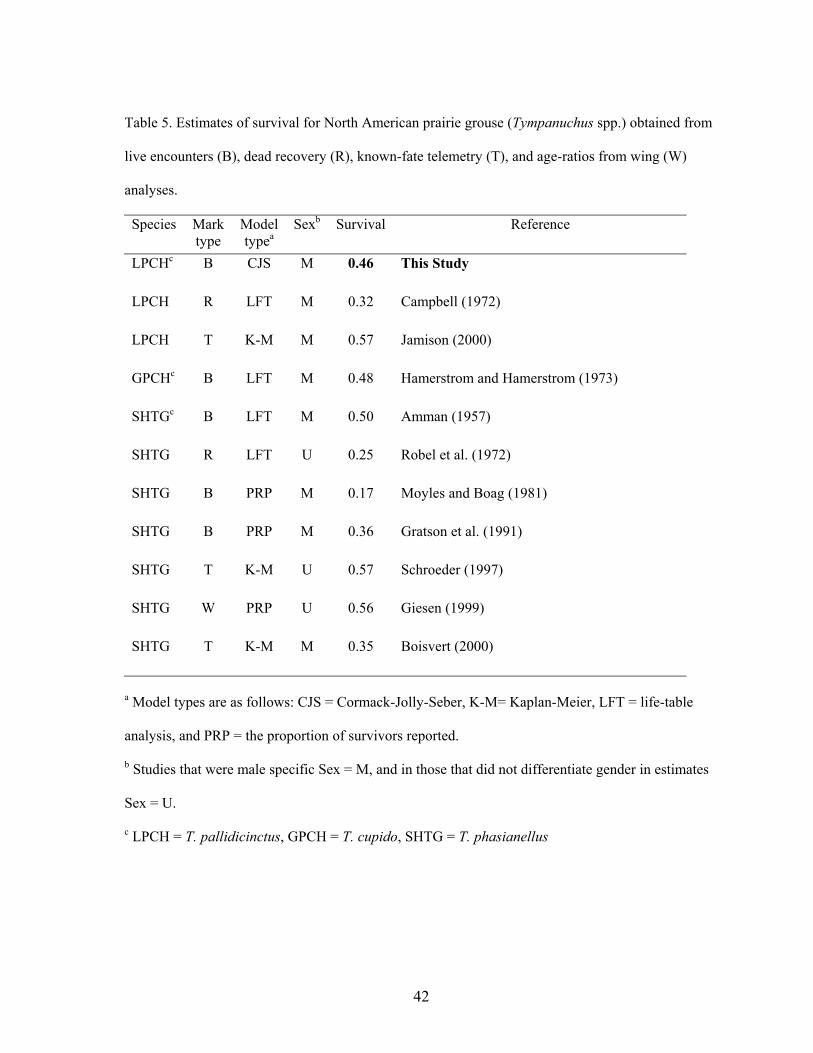
Table 5. Estimates of survival for North American prairie grouse (Tympanuchus spp.) obtained from

live encounters (B), dead recovery (R), known-fate telemetry (T), and age-ratios from wing (W)

analyses.

Species

Mark type

Model typea

Sexb Survival Reference

LPCHc B CJS M 0.46 This Study

LPCH R LFT M 0.32 Campbell (1972)

LPCH T K-M M 0.57 Jamison (2000)

GPCHc B LFT M 0.48 Hamerstrom and Hamerstrom (1973)

SHTGc B LFT M 0.50 Amman (1957)

SHTG R LFT U 0.25 Robel et al. (1972)

SHTG B PRP M 0.17 Moyles and Boag (1981)

SHTG B PRP M 0.36 Gratson et al. (1991)

SHTG T K-M U 0.57 Schroeder (1997)

SHTG W PRP U 0.56 Giesen (1999)

SHTG T K-M M 0.35 Boisvert (2000)

a Model types are as follows: CJS = Cormack-Jolly-Seber, K-M= Kaplan-Meier, LFT = life-table

analysis, and PRP = the proportion of survivors reported.

b Studies that were male specific Sex = M, and in those that did not differentiate gender in estimates

Sex = U.

c LPCH = T. pallidicinctus, GPCH = T. cupido, SHTG = T. phasianellus

42

Table 6. Estimates for age-specific survival and breeding for male grouse obtained from live encounters

(B), dead recovery (R), known-fate telemetry (T), and age-ratios from wing (W) analyses.

Age / survival rate Delayed maturation

Mating system / species

Model typea

Data 1b 2 ≥2 Refc Y Refc

Monogamous

Willow ptarmigan PRP B 0.44 NDd 0.25 5 N 5,17

Rock ptarmigan PRP B 0.24 ND 0.21 1 N 1

White-tailed ptarmigan LFT B 0.76 0.74 0.30 3 N 3

Hazel grouse K-M T 0.75 ND 0.75 21 N 18

Dispersed arena Ruffed grouse PRP B 0.41 0.42 0.44 4 Y 4

Siberian spruce grouse ND ND ND ND ND Y 19

Spruce grouse PRP B 0.92 ND 0.81 9 Y 15

Blue grouse PRP B 0.55 0.84 0.75 11 Y 11

Lek mating Greater prairie-chicken LFT B 0.50 0.48 0.41 7 Y 6,7

Lesser prairie-chicken CJS B 0.62 0.49 0.35 23 Y 23

Sharp-tailed grouse PRP B 0.39 ND 0.33 16 Y 10, 16

Black grousee K-M T 1.0 ND 0.70 9 Y 2

Greater sage-grouse REC B 0.63 ND 0.37 22 Y 8,14

Capercaillie PRP W 0.54 ND 0.46 13 Y 20

a Model types are as follows: CJS = Cormack-Jolly-Seber, K-M= Kaplan-Meier, LFT = life-table

analysis, and PRP = the proportion of survivors reported.

43

Table 6. continued b Age of birds 1 = yearling, 2 = 2 years old (adult in this study), and ≥ 2 = 2 years old or older (older

adult in this study). c References: 1, Weeden (1965); 2, Kruijt and Hogan (1967); 3, Braun (1969) 4, Gullion and Marshall

(1968); 5, Bergerud (1970); 6, Robel (1970); 7, Hamerstrom and Hamerstrom (1973); 8, Wiley (1974);

9, Keppie (1979); 10, Moyles and Boag (1981); 11, Lewis and Zwickel (1982); 12, Anglestam (1984);

13, Moss (1987); 14, Hartzler and Jenni (1988); 15, Szuba and Bendell (1988); 16, Gratson et al.

(1991); 17, Martin (1991); 18, Swenson (1991); 19, Andereev et al. (2001); 20, Storch (2001); 21,

Montadert and Leonard (2002); 22, Zablan et al. (2003); 23, This study. d ND = no data available. e Survival estimates were for breeding and summer season only.

44

CHAPTER 2

RADIOTELEMETRY ESTIMATES OF SURVIVAL IN THE LESSER

PRAIRIE-CHICKEN: ARE THERE TRANSMITTER BIASES?

Abstract: Radiotelemetry has provided wildlife biologists with a tool to estimate survival

where fate of each individual is likely known. Whereas analyses of these data can result

in highly accurate estimates, 5 assumptions must be met. Two of these assumptions, that

right-censoring is random with respect to the survival of study animal, and that

transmitters have no effect on survival of study animal, are often difficult to assess.

Using joint models developed for live encounter and dead recovery data, I examined the

potential for bias in survival estimates of radiomarked male lesser prairie-chickens in

southwestern Kansas. Additionally, I use graphing techniques to assess if the assumption

of random censoring holds in this study. In total, 201 male lesser prairie-chickens were

captured and marked during this study. Seventy-five of these birds were fitted with

radios (68 survived a 2-week acclimation period) and 126 were in the banded group.

Model selection and parameter estimation were based on the information theoretic-

approach. The model best supported by the data, Sc, pgroup+t, rg, Fc, indicated that survival

was best modeled as constant (Ŝc = 0.731, SE = 0.072) across radiomarked and banded

birds. Signal loss occurred throughout the monitoring period and appeared to be

independent of periods of high mortality. Eight of 16 (50.0, SE = 1.6 %) right-censored

birds were subsequently recaptured, which was similar to the recapture rates for known-

fate birds (23 of 52; 55.8%, SE = 0.5 %), indicating that right-censored birds had similar

survival rates to that of known-fate individuals.

45

INTRODUCTION

Radiotelemetry is widely used to collect data for estimating survival rates of

experimental treatments or groups in wildlife studies. Unbiased survival estimation

requires meeting several fundamental assumptions, 1) radioed animals are representative

(random and independent samples) of the population of interest, 2) observation periods

(or locations) are independent, 3) working radios are always located, 4) censoring is

random (i.e., any animal not located is as likely to be alive as dead), and 5) radios do not

impact survival of marked individuals (Winterstein et al. 2001). Assumptions 1 to 3 can

be met by implementing the appropriate research design. Assumptions 4 and 5 are less

controllable as the vagaries of equipment and behavior of individual animals cannot be

accounted for entirely in project design. However, assumptions 3 and 4 are closely

related as undetected individuals (i.e., vagaries of equipment) will be right-censored for a

given period. Right-censoring occurs when an individual “leaves” a study either

temporarily or permanently and the fate of the individual is unknown. Thus, all

individuals are “right-censored” at the termination of a project because, by definition,

their fate beyond that point is unknown. In practice animals are right-censored when

there is radio failure, detection rates are < 1, or there is emigration from the study area.

Often the detection of a working radio depends on the length of the observation period,

and proper planning of a project can increase the likelihood of meeting assumption 3.

Generally, researchers are faced with accepting assumptions 4 and 5 without controls to

test their validity or impact (Esler et al. 2000).

The effect of radio transmitters on survival on game birds has been well-studied,

but the results have been mixed. Most studies suffer from a lack of a suitable control

46

group and rigorous estimates of survival. Typically studies examine differences in return

rates or daily survival of birds marked with 2 or more types of harness configuration or

transmitter mass. Several studies on upland game birds provided evidence suggesting

that radios with external attachments (e.g., poncho, necklace, and backpack) had negative

impacts on survival (see review by Withey et al. 2001). In contrast, other study designs

have found no measurable effect of radios on survival or other vital rates (Hines and

Zwickel 1985, Cotter and Gratto 1995, Thirgood et al. 1995, Bro et al. 1999). Handling

effects (i.e., increased mortality immediately after handling) have occurred with early

radio designs (Marks and Marks 1987, Pekins 1988). However, the studies mentioned

above examined return rates as a measure of survival. Unfortunately return rates are

confounded by 4 probabilities: true survival (S), site fidelity (F), site propensity (γ*), and

detection (p*). Mark-recapture models can provide survival estimates while accounting

for fidelity and detection rates. However, return rates can be biologically meaningful

when a species exhibits fidelity to trapping areas (Esler et al. 2000). Currently, no studies

have examined the effects of radiomarking using contemporary analyses of capture-

recapture.

I examined the potential effect of radiomarking on survival of male lesser prairie-

chicken (Tympanuchus pallidicinctus) using a novel approach of live-recapture dead

recovery models. Typically, joint-analyses of live and dead recoveries (Burnham 1993)

have been applied to banded individuals marked-recaptured on breeding grounds and

possibly recovered during the hunting season. I expanded these joint-analyses to include

live capture and recapture of banded and radiomarked (i.e., physical recapture or

detection of transmitter signal from live radiomarked birds) individuals, and dead

47

recovery of hunter-harvested (both banded and radiomarked) and mortalities of

radiomarked individuals. I also examined the potential bias of right-censoring by

comparing the return rates of known-fate and right-censored individuals.

METHODS

Trapping, marking, monitoring

This study was conducted in native sand sagebrush prairie south of Garden City,

Kansas (37° 52′ N, 100° 59′ W) from spring 1998 to spring 2000. Lesser prairie-

chickens were captured over 3-week periods using walk-in funnel traps on leks during

spring (in late Mar to Apr) and fall (late Sep to Oct) (Haukos et al. 1991, Salter and Robel

1999). Both females and males were captured but recaptures of females were few and

this study examines only the male cohort of the radiomarked population. Captured birds

were marked with serially numbered aluminum leg bands. Relatively equal numbers of

birds were marked at all leks (n = 11) to ensure relatively equal sampling across the study

site. Birds were fitted with necklace-style radios with a mass ≤ 12 g; ≤ 1.7% of a male’s

body mass ( x = 790 g, range = 700 - 950 g). The radio transmitters had 8-month battery-

life, whip antennae, and 8 hr mortality switch. All birds that did not survive 2-weeks

post-capture (i.e., acclimation period) were included in the analysis. This conservative

approach allowed for acute effects of transmitters to be considered. Radiomarked birds

were monitored daily using a truck-mounted null-peak antenna system to ascertain their

status. For purposes of this study, the observation period was 6 months for radiomarked

birds.

48

Data analysis

I used a joint analysis for mark-recapture and staggered-entry known-fate data

from radiotelemetered and banded birds using live-recapture dead-recovery models

(hereafter joint models) (Burnham 1993) to examine the effects of radiomarking on lesser

prairie-chicken survival. My analysis included 5 encounter occasions (5 6-month

intervals between April 1998 and April 2000) and 2 attribute groups (banded or

radiomarked). Radiomarked individuals that survived a given interval and had their radio

removed at recapture (n = 11) were right-censored from the radiomarked group and

added to the banded group, and the opposite was true for banded birds that received a

radio at a subsequent interval (n = 5). When a radio signal was lost prior to a capture

period (i.e., prior to the expected life of the transmitter) they were treated as a removal

from the encounter history and right-censored.

Joint models of survival allow for combination of multiple sources of information

(Burnham 1993, Barker and White 2001). In my study, these sources of live encounter

come from 5 standard mark-recapture periods (once every 6 months) of banded birds,

“resighting” (p) periods of live radiomarked individuals, and reporting periods (r) of both

banded and radiomarked birds. Although hunter reporting of banded birds did occur, this

proportion was < 5%, but this information was included in the analysis. Thus, a

radiomarked individual may be alive and encountered, but not physically recaptured at a

given encounter period. Joint models necessarily are more complex than Cormack-Jolly-

Seber (CJS) models of live capture data (Burnham 1993). The parameters and their

definitions are as follows:

49

Si = The probability of survival; i.e., an animal that is alive at time i, is again alive at time

i + 1.

pi = The probability of detection; i.e., an animal that is alive, is at risk of capture at

trapping occasion i is captured.

ri = The probability of reporting; i.e., a marked animal that is alive at time i dies is

reported at time i + 1.

Fi = The probability of site fidelity; i.e., an animal that is at risk of capture at trapping

occasion i and is again at risk of capture at time i + 1.

Joint models of survival of banded and radiomarked individuals were analyzed

following three steps: 1) selection of the global model, 2) goodness-of-fit tests (GOF),

and 3) development of less parameterized models and model selection. Model selection

criterion was based on either Akaike’s Information Criterion adjusted for small sample

sizes (AICc), or the quasi-likelihood corrected version of AICc (QAICc). Protocols of

Burnham and Anderson (1998) were followed to identify the model best supported by the

data. Model development and parameter estimation was conducted in MARK 3.0 (White

and Burnham 1999) using design matrices and the logit link function.

I developed an a priori set of candidate models (Table 1) that allowed me to

examine the potential for the effects of radiomarking. My primary interest was

evaluating survival (S); thus, recapture (p), reporting (r), and fidelity (F) were considered

nuisance parameters. Subscripts following parameters indicate explanatory variables

(e.g., S group*t describes a model that includes both marker effect (i.e., group = marker type

banded or radiomarked) and time-dependence (i.e., survival varies by encounter

occasion) in survival. Subscript (handle) denotes different survival rate for the interval

50

after initial release or all subsequent intervals, respectively. Lastly, I used (c) to describe

models with parameters held constant (e.g., Sc, describes a model where survival is held

constant). I fitted alternative structures of F, r, and p to the global model (S group*t, pgroup+t,

rgroup, Fc) that were biologically and practically meaningful. I fixed the parameter Fc =

0.979 as only 2 of 95 (0.979) radiomarked males were known to have permanently

emigrated. Because few banded birds were reported dead, I did not consider time-

dependence in r. I assumed that behavioral differences in seasons would lead to

consistently unequal capture probabilities, p, between fall and spring encounters (Salter

and Robel 1999), and additive time structure was assumed for p under the global model.

Subsequently, time (t) and group (group) structures were fitted to p and the best structure

was selected based initially on minimum AICc. Given that the detection probabilities in p

and r of radiotelemetry (~1) and banding data (< 1) were unequal, I identified a limited

number of structures for these parameters. Specifically I did not consider models with p

and r held constant. The simplest form was with a group effect only. Survival of

radiomarked and banded birds was examined as a group effect (Sgroup). An alternative

model structure was fit to examine potential differences in handling effect for both

marker types (Sgroup, handle). This model allowed survival to vary by group effect, and for

the interval of capture to be different from later encounters.

The overall GOF of the global model was assessed using the parametric bootstrap

in MARK. The proportion of simulations (n = 1,000) that had a greater deviance than the

observed deviance provided an assessment of model fit. If this proportion was small

(<0.05) then this provides evidence that the model fits the data poorly (Cooch and White

2001). I used these simulations to estimate the degree of overdispersion (ĉ), by dividing

51

the observed deviance by the bootstrapped mean deviance. If the global model had a

poor fit, and ĉ < 3, then AICc was adjusted accordingly to this derived value of ĉ, and

QAICc used for model selection (Anderson et al. 1994).

I examined the assumption of random censoring by comparing return rates of

known-fate individuals (number alive and recaptured / number alive + number dead)

were compared to the proportion of birds that initially were right-censored, but were

recaptured or reported later (number censored and recaptured / total number censored). I

constructed a 95% confidence interval around the difference of these proportions to

determine if it was different from 0 (Agresti 1996).

I calculated an effect size (i.e., difference of means) and its 95% confidence

interval to determine if body masses differed between the 2 groups. I report sample sizes

and standard deviation along with the effect size.

RESULTS

A total of 201 male lesser prairie-chickens was captured and marked during this

study. Seventy-five of these birds were fitted with radios (68 survived the 2-week

acclimation period), and 126 were in the banded treatment group. Fall trapping resulted

in fewer birds captured per unit effort than spring trapping (Salter and Robel 1999), and

this was evident in the group and time additive (group + t) parameter structures in the

model selection below. Treatment groups were similar with respect to body mass and

age-classes. Body mass of radiomarked (n = 72, x = 790, SD = 48 g) and banded (n =

133, x = 803, SD = 44 g) birds was similar ( x difference = −12.2, CI: −25.5, 1.1 g) as

was the proportion of yearlings to adults in each sample, 0.83 and 0.79, respectively.

52

The fit of the global model (Sgroup*t, pgroup+t, rg, Fc) was rejected by the parametric

boostrap (P < 0.001), but was retained because overdispersion was minor ĉ = 2.382.

Model selection and inference were made from QAICc (Anderson et al. 1994). Some of

the overdispersion may have been due to a lack of independence, as some individuals

were in both the banded and radiomarked groups.

The model best supported by the data, Sc, pgroup+t, rg, Fc, indicated that survival

was best modeled as constant (Ŝc = 0.742, SE = 0.065) across radiomarked and banded

birds. There was some model uncertainty as ∆QAICc < 2 for the top 3 models, which

suggested that handling, S handle, pgroup+t, rg, Fc (Ŝ1 = 0.704, SE = 0.086; Ŝ2 = 0.797, SE =

0.114), and group effects, Sgroup pgroup+t, rg, Fc (Ŝradio = 0.761, SE = 0.069; Ŝband = 0.671,

SE = 0.112) may have been present (Table 1). The survival estimates from model

averaging indicated that radiomarked individuals had slightly higher survival (Ŝradio =

0.745, SE = 0.073) than banded birds (Ŝband = 0.711, SE = 0.090). Reporting rates were

higher for radiomarked birds (r = 0.636, SE = 0.157) than banded birds (r = 0.103, SE =

0.057). Recapture probabilities varied additively over time for both groups (Table 2),

and, radiomarked birds had higher overall recapture rates (pradio = 0.645, SE = 0.120;

pband = 0.303, SE = 0.124).

Effects of right-censoring

Radio signals were permanently lost for 16 birds during the 6-month sampling

intervals and were right-censored. An additional 24 radio signals were lost after the 6-

month battery life expired, and were detected as alive at last encounter occasion (this

accounts for part of known-fate percentages). Signal loss occurred throughout the

monitoring period and appeared to be independent of periods of high mortality (Fig. 1).

53

Eight of 16 (50.0, SE = 1.6 %) right-censored birds were subsequently recaptured, which

was similar (% difference = −5.8; CI: −33.8, 22.2 %) to the recapture rates for known-

fate birds (23 of 52; 55.8%, SE = 0.5 %), suggesting that right-censored birds had similar

survival rates to that of known-fate individuals.

DISCUSSION

This study found no evidence that radiomarking male lesser prairie-chickens

negatively impacted their survival. Rather, contrary to the predicted outcome,

radiomarked individuals had a slightly higher survival rate. Right-censored birds had

similar return rates when compared to those with known-fates. Inference about survival

in this group was based on relatively small sample sizes but return rates were similar

enough to provide support for a comparable mortality rate between them. I recognize

that my analyses were retrospective and an experimental design would have had greater

statistical power. However, given the positive direction of the difference between

radiomarked and banded birds, it is likely that radios had little impact on bird survival in

my study population. Inference in this study is limited to the male cohort of the

population. However, given that females average about < 70 g males, it is likely that

small transmitters (<12 g) have little impact on their survival.

Two types of transmitters

This is the first study to demonstrate that radios had no measurable effect on

prairie grouse (Tympanuchus spp.). Previous work on both sharp-tailed grouse (T.

phasianellus) and greater prairie-chickens (T. cupido) detected large negative effects of

radios on survival (Marks and Marks 1987, Burger et al. 1991). It is important to note

that Marks and Marks (1987) and Burger et al. (1991) measured the effects of the larger

54

(18-22 g) poncho-style solar powered transmitters, in contrast to the 12-g lithium battery-

powered necklace style used in my study. Marks and Marks (1987) lacked a suitable

control group (n = 9) to compare return rates or survival with the radiomarked birds (n =

36). However, 23 of 35 radiomarked birds in the Marks and Marks (1987) study

succumbed to predation, of which 65% occurred during the breeding season. Burger et

al. (1991) documented that birds marked with larger 2-stage transmitter and reflective

surface had twice the probability of being depredated than those fitted with 1-stage radios

(14 g). Similar patterns of mortality were documented for ruffed grouse (Bonasa

umbellus) and ring-necked pheasant (Phasianus colchicus), where birds marked with a

heavier backpack style transmitters had reduced survival rates (Warner and Etter 1983,

Small and Rusch 1985).

Two types of marking

Thirgood et al. (1995) found no measurable effect of radiomarking (necklace style

transmitters) on red grouse (Lagopus lagopus scoticus) when compared to patagium

tagged birds. They suggested that the miniaturization of the necklace-style transmitters

has alleviated some of the lethal effects reported earlier in other grouse species with

larger transmitters (Marks and Marks 1987, Pekins 1988). Thirgood et al. (1995)

suggested that necklace style transmitters are the preferred method for marking grouse

species. Alternatively, Caizergues and Ellison (1998) reported lower nest success rates

and smaller brood sizes of radiomarked black grouse (Tetrao tetrix) females when

compared to unmarked individuals, but they did not examine survival rates. Overall,

radiomarked females raised fewer broods than unmarked birds, but chicks per female

were nearly equal between the 2 groups (Caizergues and Ellison 1998). One limitation to

55

their study was that individuals were not individually identifiable in their unmarked

population. Thus, larger brood sizes could have been an artifact of double counting

females with large broods. The marked sample was relatively small (≤ 8 marked females

per year, n = 26 for 5 years), thus detecting annual differences in reproductive success

between groups was not possible.

The cause of marker-specific survival rates may not be easily understood as

yearly variation can impact the outcome of these studies (Cotter and Gratto 1995, Bro et

al. 1999). Years when birds may be stressed or in poor condition may increase the

negative effect of radiomarking. In my study, models with time dependency (i.e., either

Sgroup+t or Sgroup*t) in survival were not supported by the data. Although the additive

models had slightly better fit than full time-dependence, they indicated that radioed birds

on average had higher survival than banded birds.

Censoring

Random censoring is a critical assumption of telemetry studies, and violation of

the assumption can result in significant bias in Ŝ (Tsai et al. 1999, Winterstein et al.

2001). This assumption has been difficult to evaluate in the field (Esler et al. 2000). In

this study, return rates were similar between known-fate and right-censored individuals,

and the timing of censoring appeared to be independent of mortality (Fig. 1). However,

the power of my retrospective study to detect even a 10 % difference in return rates was

low (β = 0.11). Esler et al. (2000) documented a similar pattern in radiomarked harlequin

ducks (Histronicus histronicus) but also acknowledged the low power of their study

design.

56

Miniaturization and method of attaching transmitters appear to have reduced the

impact of radios on survival of prairie grouse, because survival rates of radioed birds in

my study were higher than those reported by Marks and Marks (1987) and Burger et al.

(1991). Male lesser prairie-chickens in my study were not measurably impacted by

radiomarking, as their survival rates were greater than or equal to those of banded birds.

Inference was limited to the male cohort of this population. Future work should

implement a rigorous experimental study to examine the effects of transmitters on free-

living birds and females under field conditions.

ACKNOWLEDGMENTS


Beach for access to private property. B. E. Jamison, J. C. Pitman, G. C. Salter, T. G.

Shane, and T. L. Walker, Jr., assisted with trapping and banding of prairie chickens. B.

K. Sandercock and G. C. White provided useful insights to the analysis of the joint live-

dead recovery models. Financial and logistical support was provided by Kansas

Department of Wildlife and Parks (Federal Aid in Wildlife restoration projects, W-47-R

and W-53-R), Kansas Agricultural Experiment Station (Contribution No. 03-_______),

Division of Biology at Kansas State University, and Weststar Energy Inc.

LITERATURE CITED

Agresti, A. 1996. An introduction to categorical data analysis. Wiley & Sons Inc.. New

York, New York, USA.

Anderson, D. R., K. P. Burnham, and G. C. White. 1994. AIC model selection in

overdispersed capture-recapture data. Ecology 75: 1780-1793.

Barker, R. J., and G. C. White. 2001. Joint analysis of live and dead encounters of

57

marked animals. Pages 361-367 in R. Field, R. J. Warren, H. Okarma, and P. R.

Sievert, editors. Wildlife, land, and people: priorities for the 21st century.

Proceedings from the Second International Wildlife Congress. The Wildlife

Society, Bethesda, Maryland, USA.

Bro, E., J. Clobert, and F. Reitz. 1999. Effects of radiotransmitters on survival and

reproductive success of gray partridge. Journal of Wildlife Management 63: 1044-

1051.

Burger, L. W., M. R. Ryan, D. P. Jones, and A. P. Wywialowski. 1991. Radio

transmitters bias estimation of movements and survival. Journal of Wildlife


Burnham, K. P. 1993. A theory for combined analysis of ring recovery and recapture

data. Pages 199-213 in P. North and J. D. Lebreton, editors. Marked individuals

in bird population studies. Birkhauser Verlag, Basel, Switzerland.

Burnham, K. P., and D. R. Anderson . 1998. Model selection and inference a practical


Caizerigues, A., and L. N. Ellison. 1998. Impact of radio-tracking on black grouse

Tetrao tetrix reproductive success in the French Alps. Wildlife Biology 4: 205-

212.

Carroll, J. P. 1990. Winter and spring survival of radio-tagged gray partridge in North

Dakota. Journal of Wildlife Management 54: 657-662.

Cooch, E., and G. C. White 2001. Using MARK–a gentle introduction.

http://www.cnr.colostate.edu/~gwhite/mark/mark.html (6 June 2002)

Cotter, R. C., and C. J. Gratto. 1995. Effects of nest and brood visits and radio

transmitters on rock ptarmigan. Journal of Wildlife Management 59: 93-98.

Esler, D., D. M. Mulcahy, and R. L. Jarvis. 2000. Testing assumptions for unbiased

estimation of survival of radiomarked harlequin ducks. Journal of Wildlife

58




Hines, J. E., and F. C. Zwickel. 1985. Influence of radio packages on young blue grouse.


Jamison, B. E., R. J. Robel, J. S. Pontius, and R. D. Applegate. 2002. Invertebrate

biomass: associations with lesser-prairie chicken habitat use and sand sagebrush

density in southwestern Kansas. Wildlife Society Bulletin 30: 517-526.

Marks, J. S., and V. S. Marks. 1987. Influence of radio collars on survival of sharp-tailed

grouse. Journal of Wildlife Management 51: 468-471.

Pekins, P. J. 1988. Effects of poncho mounted radios on blue grouse. Journal of Field


Salter, G. C., and R. J. Robel. 2000. Capturing lesser prairie-chickens on leks during fall.

Transactions of the Kansas Academy of Science 103: 46-47.

Small, R. J., and D. H. Rusch. 1985. Backpacks vs. ponchos: survival and movements of

radio-marked ruffed grouse. Wildlife Society Bulletin 13: 163-165.

Thirgood, S. J., S. M. Redpath, P. J. Hudson, M. M. Nichols, and N. J. Aebischer. 1995.

Effects of necklace radio-transmitters on survival and breeding success of red

grouse Lagopus lagopus scoticus. Wildlife Biology 1: 121-126.

Tsai, K., K. H. Pollock, and C. Brownie. 1999. Effects of violation of assumptions for

survival analysis methods in radiotelemetry studies. Journal of Wildlife


Warner, R. E., and S. L. Etter. 1983. Reproduction and survival of radio-marked hen

ring-necked pheasants in Illinois. Journal of Wildlife Management 47: 369-375.


59


Winterstein, S. R., K. H. Pollock, and C. M. Bunk . 2001. Analysis of survival data from

telemetry studies. Pages 351-380 in J. Millspaugh and J. Marzluff, editors. Radio

Tracking and Animal Populations. Academic Press, San Diego, California, USA.

Withey, J. C., T. D. Bloxton, and J. M. Marzluff . 2001. Effects of tagging and location in

error in wildlife radiotelemetry studies. Pages 45-75 in J. Millspaugh and J.

Marzluff, editors. Radio Tracking and Animal Populations. Academic Press,

San Diego, California, USA.

60

Table 1. Candidate live-dead recovery models for estimating survival of radiomarked

and banded lesser prairie-chickens in Finney County, Kansas, 1998-2000.

Model statisticsa

Model structureb

QAICc ∆QAICc wi K Dev

Sc, pgroup+t, rgroup, Fc 279.5 0.00 0.43 8 77.81

Sc,handle, pgroup+t, rgroup, Fc 280.8 1.36 0.22 9 77.04

Sgroup, pgroup+t, rgroup, Fc 281.1 1.65 0.19 9 77.33

Sgroup,handle, pgroup+t, rgroup, Fc 282.5 3.02 0.09 10 76.55

St, pgroup+t, rgroup, Fc 284.9 5.42 0.03 12 74.62

Sgroup + t, pgroup+t, rgroup, Fc 286.2 6.72 0.01 13 73.73

Sgroup*t, handle, pgroup+t, rgroup, Fc 287.9 8.37 0.01 18 64.23

St,handle, pgroup+t, rgroup, Fc 288.1 8.57 0.01 13 75.58

Sgroup + t ,handle, pgroup+t, rgroup, Fc 288.2 8.70 0.01 14 73.51

Sgroup, handle+ t, pgroup+t, rgroup, Fc 288.6 9.15 0.00 14 73.96

Sgroup*t, pgroup+t, rgroup, Fc 288.8 9.30 0.00 15 71.89

Sgroup + t ,handle+t, pgroup+t, rgroup, Fc 292.2 12.72 0.00 17 70.84

Sgroup* t ,handle+t, pgroup+t, rgroup, Fc 293.3 13.82 0.00 22 60.48

a Model fit is described by deviance (Dev), the number of parameters (K), quasi-Akaike’s

Information Criteria (ĉ = 2.382) corrected for small sample size (QAICc), and QAICc

weights (wi).

b Models were structured to separate survival (Ŝ), for marker effect (group) for both

radiomarked and banded males immediately after handling (handle), and survival in later

transitions. Parameter estimates include recapture rate (p), reporting rate (r), and site

fidelity (F) which was fixed at 0.979.

61

Table 2. Model averaged parameter estimates (± SE) from the 3 best (∆QAICc< 2) live-

dead recovery models of radiomarked and banded male lesser prairie-chickens in Finney

County, Kansas, 1998-2000.

Marker type

Parameter estimatesa Banded Radio

S group 0.711 ± 0.090 0.745 ± 0.073

pfall-98 0.161 ± 0.076 0.502 ± 0.129

pspring-99 0.574 ± 0.162 0.876 ± 0.071

pfall-99 0.158 ± 0.084 0.495 ± 0.137

pspring-00 0.318 ± 0.172 0.707 ± 0.145

r group 0.103 ± 0.057 0.636 ± 0.157

F 0.979 ± 0.000 0.979 ± 0.000 aParameter estimates include survival (Ŝ), recapture rate (p), reporting rate (r), and site

fidelity (F).

62

Fig 1. The cumulative frequency distribution (A) of mortalities and right-censoring

indicates that the high mortality periods (2-week intervals) were not associated with right

censoring. The distribution of mortality and right-censoring (B) indicates the actual

numbers lost to mortality or signal in a given 2-week period were not usually related.

Both figures show time (2-week periods) from capture and release.

63

10 20 30 40

Cum

ulat

ive

Freq

uenc

y D

istri

butio

n

0.0

0.2

0.4

0.6

0.8

1.0

DeadCensored

Expected date of radio failure

2

2-week periods after initial capture

10 20 30 40

Num

ber o

f bird

s

0

2

4

6

8

dead censor

Expected date of radio failure

2

(A)

(B)

64

CHAPTER 3

GENDER AND AGE-SPECIFIC SURVIVAL AND PROBABLE CAUSES OF

MORTALITY IN RADIOMARKED LESSER PRAIRIE-CHICKENS IN KANSAS

Abstract: Long-term declines in population indices and reductions in habitat have

lead to increasing concern over the status of the lesser prairie-chicken (Tympanuchus

pallidicinctus). It is essential to identify management approaches that have the greatest

positive impact on rates of population growth. I evaluated the effects of season, age, and

gender on the survival of lesser prairie-chickens in southwestern Kansas. Using data

from a 6-year field study, I estimated summer (Apr - Nov) and seasonal rates (Apr - Mar)

using known-fate (radiotelemetry) survival models. I evaluated the probable mortality

causes of radiomarked birds. In total, 136 male (46 yearling, 66 adult, 24 age

undetermined), and 227 female (87 yearling, 117 adult, and 23 age undetermined) lesser

prairie-chickens were captured and fitted with radio transmitters from 1997 to 2002. The

summer known-fate analyses revealed that overall male (Ŝ = 0.71, SE = 0.06) and female

(Ŝ = 0.69, SE = 0.06) survival rates were similar, but females were most susceptible to

mortality during May and June. Additionally, the summer analysis indicated that

yearling females had a greater probability (Ŝ = 0.77, SE = 0.06) of surviving than adults

(Ŝ = 0.62, SE = 0.05). These patterns were consistent for both the seasonal and summer

survival rates. One-hundred and thirty-four mortalities were recorded from spring 1997

to spring 2003, and 54% were attributed to mammalian predation. Generally, lesser

prairie-chickens had higher estimated survival than those reported for other prairie

grouse, suggesting that adult survival was not a limiting factor for lesser prairie-chickens

in Kansas.

65

INTRODUCTION

Seasonal survival (S) rates and the timing of mortality (1 - S) events are important

parameters in evolutionary ecology and wildlife management (Caizergues and Ellison

1997). Understanding the seasonal variation in the timing of mortality and its severity

are especially important to grouse management (Bergerud 1988), as females in

promiscuous systems (unipaternal care) may have an increased mortality risk during

incubation and brood-rearing periods. Yearling and adult females may have different

survivorship based on reproductive effort and success (Saether 1990). In general, more

experienced birds will have greater fecundity and survival, thus resulting in lower

yearling survival rates (Saether 1990).

Male and female grouse of promiscuous mating systems have different

reproductive costs. Males do not participate in nest-building, incubation, or brood-

rearing, their only contribution is gametes. However, males do incur a cost of breeding

because of conspicuous plumage and displays during territorial defense and may suffer

higher mortality than females. Females incur a cost of reproduction through egg

production, incubation, and brood rearing. Their susceptibility to predation during

incubation is thought to be higher than other times of year (Bergerud 1988). It is unclear

if a short-term decrease in female survival (reproductive cost) would yield a lower annual

survival rate than males. Is it possible that the cost of nesting and conspicuous display

will result in similar survival rates between the genders?

Differential survival in gender and age-classes may result in either skewed sex- or

age-ratios in harvest (e.g., wing or head samples) or count data (Amman 1957, Campbell

1972, Linden 1981, Moss 1987, Bergerud 1988). Survival estimates from age-ratios

66

assume stable populations, equal sampling of yearlings and adults, and a constant

mortality rate. Most survival estimates for grouse have been based on these methods

(Bergerud 1988). Given the tenuous status of many grouse populations (Storch 2000),

more accurate estimates are needed for conservation actions. Radiotelemetry may

provide accurate parameter estimates if the basic assumptions are met (Winterstein et al.

2001).

Little is known about seasonal or annual survivorship of lesser prairie-chickens

(Tympanuchus pallidicinctus), but such information is critical for this species of

conservation concern. It is currently listed as a “warranted but precluded” threatened

species (U.S. Fish and Wildlife Service 2002). Band recovery data from hunters in New

Mexico were used to estimate an annual survival rate of 35% (Campbell 1972), and

Merchant (1982) estimated a 6-month survival rate of 59% (extrapolated 12-month

survival = 35%) for radiomarked females that included the nesting and brood rearing

periods. In Kansas, Jamison (2000) estimated annual survival of radiomarked males to

be 57%. Six-month (Apr-Sep) survival rates were estimated at 74% for males and

females during the same study (Jamison 2000). This estimate extrapolated to 12 months

would be approximately 55%. However, lower survival rates of females than males have

been implicated in biased sex-ratios (Campbell 1972); there is little evidence to support

this idea. The available information on lesser prairie-chicken survival is incomplete, as

there are few annual estimates, and no information on the timing of mortality for females

and males during a year. Such information is imperative for conservation efforts (e.g.,

population viability analyses, harvest regulations) and basic ecological understanding.

67

Using radiotelemetry data from 1997 to 2003, I address 3 research hypotheses and

provide a description of probable mortality causes of the lesser prairie-chicken. I

examined survival in terms of an overall rate (9 and 12-month periods for males and

females) to identify potential cumulative effects of gender-specific costs of reproduction.

I quantified the timing of mortality events for males and females to verify the costs of

reproduction hypothesis (i.e., did both males and females suffer the lowest survival rates

during the breeding season?). Thus, if the cost of reproduction hypothesis is supported

then timing may not differ but the overall survival rate will differ. I estimated survival

for yearling and adult females to determine if age-structured survival was evident in the

population. Here, I test the constraint hypothesis, which argues that yearlings lack some

of the skills essential for high reproductive performance. Because high reproductive

performance is often linked to survival (Saether 1990), I used survival and ancillary data

on reproductive rates to evaluate this hypothesis. Lastly, I evaluated the probable

mortality causes of radiomarked birds.

METHODS

Study area

The study region was comprised of 2 fragments (~5000 ha each) of native

sandsage (Artemisia filifolia) prairie near Garden City, Finney County, Kansas (37° 52′

N, 100° 59′ W). Work began on Area I (southwest of Garden City) in 1997. In 2000,

trapping and monitoring efforts were expanded to include Area II (southeast of Garden

City). Prior to 1970, these 2 areas were part of a contiguous tract of native sandsage

prairie. The development of center pivot irrigation led to the conversion of much of the

sandsage prairie to intensive agriculture (Waddell and Hanzlick 1978), and left these

68

areas as 2 fragments with about 19 km of agricultural fields between patch centroids

(Hullett et al. 1988, Jamison 2000).

Capture, marking, and monitoring

Lesser prairie-chickens were captured on 20 leks using walk-in funnel traps

(Haukos et al. 1991, Schroeder and Braun 1991) primarily during spring, and a subset of

leks during the fall of 1998 and 1999 for a related study (Salter and Robel 1999, Chapter

2). Spring trapping began the last week of March and continued into the second week of

April. Fall trapping lasted approximately 3 weeks in late September and early October.

Traps were placed on all known leks (>2 displaying males) found in native prairie on the

study sites. Once captured, birds were aged as yearling (~10 months of age) or adult (≥

22 months) based on shape, wear, and coloration of the 9th and 10th primaries (Amman

1944, Copelin 1963). Age was not recorded during the first year of the study (1997).

Gender of mature birds was determined by the patterns on tail and crown feathers

(Amman1944, Copelin 1963). Body mass was measured (± 2.5 grams) using a Pesola

spring scale.

Birds were individually marked with numbered aluminum leg bands.

Radiomarked birds were fitted with a lithium battery-powered necklace-style transmitter

(≤ 12-g), which was ≤ 1.9 % of a bird’s body mass (sexes pooled, x = 783, range = 630-

890 g) and below the recommended 3 % maximum level (Withey et al. 2001).

Transmitters had either an 8- or 12-hour mortality switch, and a 6- (1997-1999) or 12-

month (2000-2003) battery life. Nearly all captured females were marked with radio-

transmitters, but only a subset of males was marked in a given year. For these samples,

69

workers attempted to distribute the radios evenly across the study areas, by placing

roughly equal numbers on males on each lek trapped.

Radiomarked birds were monitored daily with a vehicle-mounted null-peak twin

Yagi antenna system. Once a mortality switch had been activated on a transmitter, the

unit was relocated and retrieved with a hand-held Yagi in < 12-hrs. Aerial surveys from

fixed wing aircraft were conducted at least once a month to locate undetected signals.

Once located by air, previously undetected birds that had emigrated from the primary

study areas were subsequently relocated approximately every 10 days from truck-

mounted systems.

Probable causes of mortality

When a carcass or kill site was located, the probable cause of mortality was

determined as mammal, avian, accident, hunter, snake, or unknown based on the

evidence at the recovery site. Scavenging of carcasses was possible but was potentially

minimized because of quick recovery of transmitters on a mortality pulse. It is difficult

to make unambiguous statements about causes of mortality because of potential

scavenging or confounding evidence at a recovery site (Bumann and Stauffer 2002).

Thus, I refer to probable causes of mortality in this paper.

A mortality event was classified as mammalian predation if one of the following

was evident at the kill site: bite marks on the transmitter, chewed feathers and/or

aluminum band in addition to tracks or mammalian scat at the recovery site. Coyote

(Canis latrans), American badger (Taxidea taxus), and bobcat (Lynx rufus) were all

possible mammalian predators. Carcasses that had been decapitated and/or cleaned of the

breast muscle with no apparent chewing, the presence of white wash, or plucking were

70

classified as avian predation. Accidental deaths were carcasses recovered near a

powerline, fenceline, or dismembered by farm machinery that had no apparent marks of

predation. Hunter recoveries of banded birds were reported as such. Often these were

not radiomarked birds, but are included here to provide an estimate of hunter harvest.

Snake predation was rare, but evidenced by feathers matted with saliva or residue from

the head to just above the furcula. Unknown causes included mortalities that went

undetected for more than 2 days, carcasses with confounding signs at the recovery site

(e.g., mammalian chew marks on feathers, etc., and under a powerline), or in the event a

carcass was recovered unscathed. Likelihood-ratio tests (G2) were used to examine the

differences in mortality causes between males and females.

Survival modeling

Known-fate survival modeling requires that 6 assumptions be met: the animals

marked are a random sample from the population, the experimental units (e.g., marked

animals) are independent, observation periods are independent, working radios are

always located, right-censoring is random, and that radios do not impact survival

(Winterstein et al. 2001). Right-censoring occurs when an individual “leaves” a study

either temporarily or permanently and the fate of the individual is unknown.

I must assume that captured females were a random subset of the population as all

captured females were marked. This assumption holds if nearly all females attend leks in

the spring for breeding. Males were marked so that an equal number from each lek were

monitored. To reduce bias in sampling, all leks were trapped on our study areas over a

relatively short period. Birds were tracked daily to enhance the detection probability of

functioning radios and transmitters with a mortality pulse (detection distance was ~1.6

71

km). Although an individual may have been missed for a day or so, birds that had not

permanently emigrated were found within a weekly sampling period. I modeled survival

with time units ≥ 1 week as these were more likely to be independent given that I

estimated survival over 9- and 12-month periods. Month was the base time unit for the

12-month estimates as aerial surveying was conducted monthly from September 2002

through March 2003. Birds were right-censored from the encounter histories if they were

known to emigrate or if a radio signal was lost. A 2-year comparison of survival rates of

radiomarked and banded birds from our study area found no measurable effect of

radiomarking (Chapter 2). I used a staggered entry known-fate encounter history and

included individuals after a 2-week acclimation (Winterstein et al. 2001) to the radio-

collar. Most birds would have entered the encounter history once our trapping efforts had

ceased. In fact, most mortality that occurred during the trapping season was excluded

from the analysis.

I estimated survival rates using known-fate models in MARK 3.0 (White and

Burnham 1999). Models were developed using the design matrix feature and a logit link

function. Global models were the most highly parameterized model, but not necessarily

saturated models. Model goodness-of-fit was evaluated by examining residual plots.

Model selection was based on the minimization of Akaike’s Information Criterion

corrected for small samples sizes (AICc), and AICc weights (wi’s) to select the model best

supported by the data. I used multi-model inference and model averaging in cases where

the difference in AICc values (∆AICc) between the best and subsequent models was < 2

(Burnham and Anderson 1998). Model averaging was used to refine parameter estimates

from candidate sets with several competing models. In this procedure, parameter

72

estimates (i.e., survival and standard errors) are calculated as a weighted mean using

AICc weights.

Data sets and candidate models

Transmitters in this study had different expected battery life; those used from

spring 1997 through fall 1999 had maximum life of 6 to 9-months (hereafter summer),

and those used from 2000 to 2003 had approximately a 12-month maximum life

(hereafter seasonal) (Table 1). I used the summer data to increase sample size of cohorts

across years (Table 1). However, these data may be biased if used to extrapolate to 12-

month survival estimates as they exclude winter survival. The bias could be positive if

winter survival is appreciably greater than the previous 8 months. Therefore, I analyzed

the seasonal data as a verification of the results from the summer analyses. In both sets

of analyses, data were pooled across various cohorts (Table 1) in order to have sufficient

sample sizes (n ≥ 25) to detect differences in timing and overall survival rates across

groups (Winterstein et al. 2001). Admittedly, such pooling may weaken the power of the

analyses, as there could have been confounding factors.

RESULTS

In total, 781 lesser prairie-chickens were captured during the 6-year study. Of

these, 136 males (46 yearling, 66 adult, 24 age undetermined) and 227 females (87

yearling, 117 adult, and 23 age undetermined) were fitted with radio-transmitters (Table

1). Fifteen birds (4%) (8 males and 7 females) died within the 2-week adjustment period

after marking. Birds were right-censored (30.8 %; 112 of 363 radiomarked individuals)

because of collar slippage and radio failure (79.5 %; 89 of 112), and emigration (20.5 %;

23 of 112) to other sagebrush fragments.

73

Summer survival

Monthly variation in survival was an important structure to all candidate sets, as

either an additive or a main effect (Table 2). Much of the time dependent variation was

centered on the nesting season (Fig. 1). Yearly variation in female summer survival was

well supported by the data (wi = 0.60), as summer survival (Ŝ) varied from 0.537 to 0.866

between 1997 and 2002 (Table 3). Age-specific survival of females with an additive

monthly effect (Fig. 1) was reasonably well supported by the data (wi = 0.54); however,

monthly variation alone fit nearly as well (∆AICc = 0.74; wi = 0.38) (Table 2). Yearling

females survived at a slightly higher rate (Ŝ = 0.757, SE = 0.041) than adult females (Ŝ =

0.692, SE = 0.041) during the summer (Table 3). Overall the monthly timing of mortality

(Fig. 2) and survivorship for males (Ŝ = 0.692, SE = 0.050) and females (Ŝ = 0.666, SE =

0.053) were similar, as time dependent and constant survival models fit better than those

with gender effects. There were several competing models in this candidate set, as the

top 5 models all had ∆AICc < 2 and wi‘s ranging from 0.13 to 0.29 (Table 2). However, a

plot of biweekly survival for each gender (Fig. 2) indicated that female survivorship was

inversely related to the cumulative number of females incubating nests, and increased as

nesting activities ceased. Alternatively, male survivorship appeared to decrease

periodically during the breeding season (Fig. 2).

Seasonal survival

Monthly variation was also important in model selection of the seasonal data, as

month was in the top 2 models of each candidate set (Table 4). Gender- and time-

specific survival was the most parsimonious model; however, the timing of mortality may

have been more important (Fig. 3) as the probability for males (Ŝ = 0.39 SE = 0.10) to

74

survive 12-months was similar to that of females (Ŝ = 0.43 SE = 0.05) (Table 5). Age-

specific survival with an additive time effect for females was well supported; however,

monthly variation alone was a highly comparable model (w1/w2 = 1.2; Table 4). The

probability of yearling females surviving the interval was substantially higher (Ŝ = 0.52

SE = 0.08), than that of adults (Ŝ = 0.37 SE = 0.06), but the difference in these

probabilities estimated from model averaging was less than non-averaged estimates

(Ŝyearling = 0.48 SE = 0.06; Ŝadult = 0.40 SE = 0.05)(Table 5). Monthly variation in

survival (Fig. 3) indicated that the greatest mortality occurred during the reproductive

season (Ŝ for Apr – Jul = 0.69, SE = 0.04), but winter survival (Nov – Feb) was not much

higher (Ŝ = 0.77, SE = 0.06).


One-hundred and thirty four mortalities were recorded from spring 1997 to spring

2003 (Table 6). The majority of mortality was attributed to mammalian predation (54%).

It is likely that coyotes were the primary mammalian predator, as most sign at recovery

locations suggested canid predation. Five whole carcasses were cached under shrubs, but

could only be classified as mammalian predation. Most of the mammalian predation

(75%) was associated with female mortality (G2 = 4.96, df =1, P = 0.004) and coincided

with losses during nesting (>30%).

Raptor predation occurred primarily during spring and winter, which coincided

with presence of wintering or migratory populations of red-tailed hawk (Buteo

jamaicensis), ferruginous hawk (Buteo regalis), rough-legged hawk (Buteo lagopus),

northern harrier (Circus cyaneus), and a few prairie falcons (Falco mexicanus). Great-

horned owls (Bubo virginianus) were present year round and were probable predators;

75

however, with no raptor predation in summer it is thought that their role as a predator was

minimal. Males seemed more susceptible to raptor predation (20%) than females (11%),

but this rate was not measurably different (G2 = 1.88, df =1, P = 0.170). Seven of the 8

accidents were associated with powerline collisions, and one female was killed by farm

machinery while incubating a nest in an alfalfa field. Snakes were responsible for the

mortalities of 3 nesting females. These females were > 20 days into incubation when

they were killed, and were likely tenacious in defending the nest. The gopher snake

(Pituophis catenifer) was the probable predator as this species was observed depredating

the eggs at 4 nests, and is the only snake on the study area large enough to constrict and

attempt to swallow the head and neck of a female. Losses to recreational hunting were

small (5%) relative to the radiotelemetry population, but even less (1.2% of 655 birds)

when compared to banded birds (781[total banded]−126[known mortalities] = 655) that

were available for harvesting. Males apparently were more susceptible (15%; 7 of 44) to

hunting losses than females (1%; 1 of 90) (G2 = 8.74, df =1, P = 0.003)

DISCUSSION

Yearly variation in summer survival was evident and seemed to be highly related

to mortality rates of incubating females on nests (Fig. 1); >30% of all female mortality

was associated with the nesting period. Summer survival rates and apparent nest success

(number of nests hatching >1 egg / total number of nests) from 5 years revealed the

strength of this relationship (Fig. 4). Changes in predator communities and/or residual

cover may have influenced nest success and/or female losses (Bergerud 1988), but such

factors were not measured in this study. However, management efforts that would

increase nesting success may markedly increase annual female survival.

76

Gender-specific survival

Gender-specific survival was not well supported by the data, as the overall

survival rates of males and females were similar in the summer and seasonal analyses.

However, the timing of survival over 12 months suggested that seasonal patterns in male

survivorship do not match the temporal pattern seen in females. The conspicuous

displays (or its physiological costs) of males may increase their vulnerability in both

spring and fall thereby equalizing the female losses during nesting (Amman 1957). This

result contradicts Bergerud’s (1988) prediction that uniparental care will result in greater

mortality in females than males.

If sexually selected characters increase mating success (e.g., conspicuous plumage

or behavior), then characters that increase survival (e.g., cryptic plumage or behavior)

should make a relatively small contribution to total fitness (Angelstam 1984). In grouse,

this should result in a lower survival rate in males (the gender with sexually selected

traits in this case) than females. One might expect this pattern to be evident in the most

sexually dimorphic species, capercaillie (Tetrao urogallus), greater sage-grouse

(Centrocercus urophasianus), blue grouse (Dendragopus obscurus), and black grouse

(Tetrao tetrix). Several studies have examined annual survival rates in male and female

grouse and the results have been mixed. Greater sage-grouse are the only species in this

group in which males have lower survival rates than females (Zablan et al. 2003). Less

sexually dimorphic species, white-tailed ptarmigan (Lagopus leucurus) and spruce grouse

(Falcipennis falcipennis) also exhibit gender-specific patterns of survival (Choate 1963,

Braun 1969, Ellison 1974, Keppie 1979), but the white-tailed ptarmigan are socially

77

monogamous. However, capercaillie exhibit the inverse with males having markedly

higher survival in 4 regions of Europe (Storch 2001), and male black grouse survival is ≥

to that of females (Angelstam 1984, Caizergues and Ellison 1997). Survival rates of male

blue grouse, greater prairie-chicken (Tympanuchus cupido), sharp-tailed grouse

(Tympanuchus phasianellus), lesser prairie-chicken, hazel grouse (Bonasa bonasia),

ruffed grouse (Bonasa umbellus), and rock ptarmigan (Lagopus lagopus) are nearly equal

to those of females (Weeden 1965, Elliot and Bendell 1967, Gullion and Marshall 1968,

Hamerstrom and Hamerstrom 1973, this study).

The lack of a consistent pattern across studies makes it difficult to draw

conclusions about the role or presence of gender-specific survival rates, and to account

for markedly different investments in breeding strategies between males and females

(Bergerud 1988). The relatively equal survival rates of male and female lesser prairie-

chickens suggest that the cost of reproduction has balanced female losses during nesting

with male mortality during display and at other times of year. Alternatively, the similar

plumages between males and females may equalize the survival rates when males are not

displaying. Additionally, these comparable survival rates contradict the idea that male

biased sex-ratios are a result of differential survival (Amman 1957, Campbell 1972, Moss

1987, Linden 1981, Bergerud 1988), suggesting that such ratios may reflect a bias for

males to be susceptibile to hunter harvest. While speculative, this conclusion is

supported by the fact that 7 of 8 hunter harvested birds in this study were males. Taylor

and Guthery (1980) documented that male lesser prairie-chickens visited grain fields in

flocks, and females did so in singles. Because the common method of hunting prairie

78

chickens involves pass-shooting flocks coming into grain fields, there is some support for

this claim.

Age-specific survival

Age-specific patterns in female survival were evident in both analyses with

yearling birds surviving at a higher rate than adults. This was surprising given that

yearlings of other grouse species tend to have reduced survival and reproductive output

(Bergerud 1988, Saether 1990). However, the timing of mortality was consistent

between these groups as models with an additive time effect (Sage + month) were the most

parsimonious in both sets of analyses, with the lowest survival rates during the nesting

and brooding periods. One might predict that the cost of reproduction would result in

reduced survival rates of adults, if they had higher reproductive output. However,

reproductive parameters were similar between age-classes in this study (Fig. 5), except

that yearling nest success, 33% (SE = 5 %), was marginally higher than adults, 28% (SE

= 4%). Whereas rates of nest loss were comparable, mortality rates were not. The reason

for such differences suggests different responses to depredation events on adults and

yearlings. Adult females may have been more tenacious (i.e., a fight response) in nest

guarding (see Hannon and Smith 1987), whereas the yearlings may have had a flight

response to nest predators. If true, this could explain the lower survival rate for adult

females.


Predator classification from evidence at kill sites may be problematic, because

mammalian scavengers may be most abundant in a region (Bumann and Stauffer 2002).

Overestimation of mammalian-kills increases as a function of ambient temperature, and

79

could have occurred in this study. However, if a positive bias occurred in this study it is

likely that it was consistent for both males and females. Thus, the magnitude of the

difference in cause specific mortality rates should be a reasonable index to compare

proportional losses between males and females.

The probable causes of mortality lesser prairie-chickens differed somewhat

between males and females, as 60% of predation on females was classified as

mammalian, 1.5 times as much as males (40%). Conversely, male losses (20%) were

classified as raptor predation more so than females (11%). This potential difference is

likely from the types of predators cueing on breeding and nesting behaviors of males and

females, respectively. Northern harriers have been documented harassing and killing

prairie grouse (Berger et al. 1963, Toland 1985, Haukos and Broda 1989). The

susceptibility of males to mortality may not occur at the lek site (Berger et al. 1963), but

the physiological cost of display (Vehrencamp et al. 1989) may increase the probability

of predation both during and after breeding season (Angelstam 1984). Mammalian

predation of displaying birds is probably rare (Hamerstrom et al. 1965), and this pattern

was likely true in my study. Spring and fall raptor migrations coincided with display

activities of lesser prairie-chickens in this study, thus likely increasing their susceptibility

to raptor predation.

In 2001, 2 females died of unknown causes during the nesting season. Each

carcass was recovered intact and with a brood patch (i.e., an area of the ventral surface of

the abdomen that a female will pluck to line the nest with feathers). One hen had been

incubating for 12 days at the date of death. The other had not been located on a nest

although her radiolocations suggested she had been laying eggs for ≥ 8 days. These birds

80

were submitted for necropsy at the Diagnostic Laboratory, Kansas State University,

College of Veterinary of Medicine. Avian cholera (Pasturella mutlicoda), was isolated

from various tissues of 1 female, and was suggested to be the cause of death.

Accidental death due to powerline and/or fence collisions has a substantial impact

on populations of European grouse (Miquet 1990, Bevanger 1995, Moss et al. 2000).

Powerline collisions occurred as birds were leaving the prairie to forage in adjacent

agricultural fields. This loss appeared to be relatively small in my study population,

accounting for 5% of all mortality, similar to rates estimated for greater sage-grouse in

Idaho (Connelly et al. 2000). It is possible that some portion of the “unknown” category

was associated with powerline collisions, thus 5% may be a conservative estimate.

Powerline densities were relatively low on the study area as they usually traversed a

partial length of the prairie edge (< 40 % of 100 km of edge).

Hunting mortality was low in this study of radiomarked birds (≤ 5%) and even

less for all birds (<1.5 %). Research on European grouse suggests that hunting mortality

of <10% should not impact spring breeding populations (Ellison et al. 1988, Ellison

1991a, b). Ellison (1991a) suggested that even declining populations can sustain some

harvest (~5%) without negatively impacting production. Alternatively, Small et al.

(1991) found that hunting mortality of 20% was mostly additive to both adult and

juvenile ruffed grouse. Connelly et al. (2000) suggested that harvest of females was

additive to over-winter mortality, but that some level of exploitation (~10 %) was

tolerable given the high annual variability in hunter success. Recreational hunting losses

appeared to have minimal impact on the study population in reducing either annual

survival or numbers of breeding birds in the spring.

81

MANAGEMENT IMPLICATIONS

Management of lesser prairie-chickens should focus on habitat manipulations that

increase nest survival and decrease female losses during incubation. In fragmented

populations, predator control may achieve short-term goals of increased female survival

and nest success, but may be too costly to sustain in the long-term (Schroeder and

Baydack 2001). Long-term management should focus on creating nesting habitat that

decreases losses to mammalian predation. Similarly, experimental work is needed to

understand the mechanisms by which mammalian predators search and find nests.

Specifically identifying habitat structure that lowers the success of nest predators on nests

and on females would be most advantageous for long-term habitat management.

Limiting harvest probably would have little impact on the lesser prairie-chickens in

Kansas since most mortality occurs during the nesting season. However, more accurate

information is needed on harvest rates throughout lesser prairie-chicken range. Current

harvest levels are estimated indirectly through mail surveys to upland gamebird hunters,

who may not actually hunt prairie chickens. A free permit system specific to prairie

chicken hunters would facilitate a direct measure of hunter harvests.

ACKNOWLEDGMENTS


Beach for property access. B. E. Jamison, C. G. Griffin, J. C. Pitman, G. C. Salter, T. G.

Shane, T. L. Walker, Jr., and T. J. Whyte assisted with trapping and radiomarking of

prairie chickens. B. E. Jamison was instrumental in developing the initial candidate set

of survival models. Financial and logistical support was provided by Kansas Department

of Wildlife and Parks (Federal Aid in Wildlife restoration projects, W-47-R and W-53-

82

R), Kansas Agricultural Experiment Station (Contribution No. 03-_______), Division of

Biology at Kansas State University, and Westar Energy Inc.

LITERATURE CITED

Amman, G. A. 1944. Determining the age and sex of pinnated and sharp-tailed grouse.


Amman, G. A. 1957. The prairie grouse of Michigan. Department of Conservation Game

Division. Lansing, Michigan, USA.

Angelstam, P. 1984. Sexual and seasonal differences in mortality of black grouse Tetrao

tetrix in boreal Sweden. Ornis Scandinavica 15: 123-134.

Bendell, J. F., and P. W. Elliot. 1967. Behavior and the regulation of numbers in blue grouse.

Canadian Wildlife Service. Report Series Number 4. Ottawa, Ontario, Canada.

Berger, D. D., F. Hamerstrom, and F. N. Hamerstrom. 1963. The effect of raptors on prairie

chickens on booming grounds. Journal of Wildlife Management 27: 778-791.

Bergerud, A. T. 1970. Population dynamics of the willow ptarmigan Lagopus lagopus alleni

L. in New Foundland 1955 to 1965. Oikos 21: 299-325.

Bergerud, A. T. 1988. Population ecology of North American grouse. Pages 578-685 in A.

T. Bergerud and M. W. Gratson, editors. Adaptive Strategies and Population Ecology

of Northern Grouse. Wildlife Management Institute, Washington DC, USA.

Bevanger, K. 1995. Estimates of population consequences of tetraonid mortality caused by

collisions with high tension power lines in Norway. Journal of Applied Ecology 32:

744-753.

Boisvert, J. H. 2002. Ecology of Columbian sharp-tailed grouse associated with Conservation

Reserve Program and reclaimed surface mine lands in northwestern Colorado. Thesis,

University of Idaho, Moscow, Idaho, USA.

83

Braun, C. E. 1969. Population dynamics, habitat, and movements of white-tailed ptarmigan

in Colorado. Dissertation, Colorado State University, Fort Collins, Colorado, USA.

Bumann, G. B., and D. F. Stauffer. 2002. Scavenging of ruffed grouse in the Appalachians:

influence and implications. Wildlife Society Bulletin 30: 853-860.

Burnham, K. P. and D. R. Anderson. 1998. Model selection and inference: a practical


Caizerigues, A., and L. N. Ellison. 1998. Impact of radio-tracking on black grouse Tetrao

tetrix reproductive success in the French Alps. Wildlife Biology 4: 205-212.

Caizerigues, A., and L. N. Ellison. 1997. Survival of black grouse Tetrao tetrix the French

Alps. Wildlife Biology 3: 177-186.

Campbell, H. 1972. A population study of lesser prairie-chickens in New Mexico. Journal of


Choate, T. S. 1963. Habitat and population dynamics of white-tailed ptarmigan in Montana.


Connelly, J. W., A. D. Apa, R. B. Smith, and K. P. Reese. 2000. Effects of predation and

hunting on adult sage grouse Centrocercus urophasianus in Idaho. Wildlife Biology

6: 227-232.



USA.

Ellison, L. N. 1974. Population characteristics of Alaskan spruce grouse. Journal of Wildlife


Ellison, L. N. 1991a. Shooting and compensatory mortality in tetraonids. Ornis Scandinavica

22: 229-240.

Ellison, L. N. 1991b. Under what conditions can shooting of declining species of tetraonids

84

be justified in France? Gibier Faune Sauvage 8: 353-365.

Ellison, L. N., P. Leonard, and E. Menoni. 1988. Effect of shooting on a black grouse

population in France. Pages 117-128 in M. Spagnesi and S. Toso, editors. Acts of

First National Conference of Game Biologists.

Gullion, G. W., and W. H. Marshall. 1968. Survival of ruffed grouse in a boreal forest. The

Living Bird 7: 117-167.

Hamerstrom, F., D. D. Berger, and F. N. Hamerstrom. 1965. The effect of mammals on

prairie chickens on booming grounds. Journal of Wildlife Management 29: 536-542.

Hamerstrom, F. N., and F. Hamerstrom. 1973. The prairie chicken in Wisconsin. Wisconsin

Department of Natural Resources. Technical Bulletin No. 64. Madison, Wisconsin,

USA.

Haukos, D. A., and G. S. Broda. 1989. Northern harrier predation of lesser prairie-chicken.

Journal of Raptor Research 23: 182-183.



Hulett, G. K., J. R. Tomelleri, and C. O. Hampton. 1988. Vegetation and flora of a sandsage

prairie site in Finney County, southwestern Kansas. Transactions of the Kansas

Academy of Science 91: 83-95.


selection and movement of males in fragmented landscapes of southwestern Kansas.

Thesis, Kansas State University, Manhattan, Kansas, USA.

Keppie, D. M. 1979. Dispersal, overwinter mortality, and recruitment of spruce grouse.


Lindén, H. 1981. Estimation of juvenile mortality in the capercaillie, Tetrao urogallus, and

the black grouse, Tetrao tetrix, from indirect evidence. Finnish Game Research 39:

85

35-51.

Merchant, S. S. 1982. Habitat use, reproductive success, and survival of female lesser prairie-

chickens in two years of contrasting weather. Thesis, New Mexico State University,

Las Cruces, New Mexico, USA.

Miquet, A. 1990. Mortality in black grouse Tetrao tetrix due to elevated cables. Biological

Conservation 54: 349-355.

Moss, R. 1987. Demography of capercaillie Tetrao urogallus in northeast Scotland. II. Age

and sex distribution. Ornis Scandinavica 18: 135-140.

Moss, R., N. Picozzi, R. N. Summers, and D. Baines. 2000. Capercaillie Tetrao urogallus in

Scotland-demography of a declining population. Ibis 142: 259-267.

Saether, B. E. 1990. Age-specific variation in reproductive performance of birds. Current


Salter, G. C., and R. J. Robel. 2000. Capturing lesser prairie-chickens on leks during fall.

Transactions of the Kansas Academy of Science 103: 46-47.

Schroeder, M. A., and R. K. Baydack. 2001. Predation and the management of prairie

grouse. Wildlife Society Bulletin 29: 24-32.

Schroeder, M. A., and C. E. Braun. 1991. Walk-in funnel traps for capturing greater prairie-

chickens on leks. Journal of Field Ornithology 62: 378-385.

Small, R. J., J. C. Holzwart, and D. H. Rusch. 1991. Predation and hunting mortality of

ruffed grouse in central Wisconsin. Journal of Wildlife Management 55: 512-520.

Toland, B. 1985. Northern harrier predation of greater prairie-chickens in southwest

Missouri. Journal of Raptor Research 19: 146-148.

Vehrencamp, S. L., J. W. Bradbury, and R. M. Gibson. 1989. The energetic cost of display

in male sage grouse. Animal Behaviour 38: 885-896.

86

Waddell, B., and B. Hanzlick. 1978. The vanishing sandsage prairie. Kansas Fish and Game

Magazine1-4.

Weeden, R. B. 1965. Breeding density, reproductive success, and mortality of rock ptarmigan

at Eagle Creek, central Alaska from 1960 to 1964. Transactions of the North

American Wildlife and Natural Resources Conference 13: 336-348.





Marzluff, editors. Radio Tracking and Animal Populations. Academic Press,

San Diego, California, USA.

Winterstein, S. R. 1992. Chi-square tests for intrabrood independence when using the

mayfield method. Journal of Wildlife Management 56: 398-402.

Zablan, M. A., C. E. Braun, and G. C. White. 2003. Estimation of greater sage-grouse

survival in North Park, Colorado. Journal of Wildlife Management 67: 144-154.

87

Tabl

e 1.

Num

bers

of y

earli

ng (Y

) and

adu

lt (A

) les

ser p

rairi

e-ch

icke

ns ra

diom

arke

d in

Fin

ney

Cou

nty,

Kan

sas 1

997-

2002

.

M

ales

Fem

ales

Yea

r

Are

aI

Mon

ths

n (Y

,A)

a A

rea

II

n (Y

,A)

Mon

ths

Are

a I

n (Y

,A)

Mon

ths

Are

aII

n (Y

,A)

Mon

ths

1997

-199

8

24 (n

o-ag

e) b

9

ND

c N

D23

(no-

age)

b,d

9N

DN

D

1998

-199

9 34

(17,

17)

b

12h

ND

N

D

23

(18,

5) b

,d,e

9N

DN

D

1999

-200

041

(18,

23)

b12

h

ND

N

D

34

(18,

16)

b,d

,e9

ND

ND

2000

-200

1 N

D

ND

12

(5, 7

) g

12

26

(7, 1

9) d

,e,f,

g 12

25

(11,

14)

e,f,g

12

2001

-200

22(

0, 2

) g

12

13 (6

, 7) g

12

33 (1

2, 2

1) d

,e,f,

g 12

23

(8, 1

5) e

,f,g

12

2002

-200

3N

DN

DN

DN

D

14 (3

, 11)

d,e

,f,g

12

26 (1

0, 1

6) e

,f,g

12

Tota

ls

101(

35, 4

2 )

ND

25

(11,

14)

N

D

15

3 (5

8, 7

2)

ND

76

(29,

45)

N

D

88

a Max

imum

bat

tery

life

and

trac

king

per

iod

in m

onth

s for

a g

iven

coh

ort.

b Coh

orts

use

d to

exa

min

e se

x-sp

ecifi

c ra

tes f

or 9

mon

th p

erio

d; a

ges a

nd y

ears

poo

led.

c N

D =

no

data

ava

ilabl

e.

d Coh

orts

use

d to

exa

min

e an

nual

var

iatio

n in

surv

ival

rate

s for

9 m

onth

per

iod;

age

s poo

led.

e C

ohor

ts u

sed

to e

xam

ine

age-

spec

ific

rate

s in

fem

ales

for 9

mon

th p

erio

d; a

reas

and

yea

rs p

oole

d.

f Coh

orts

use

d to

exa

min

e ag

e-sp

ecifi

c ra

tes i

n fe

mal

es fo

r 12

mon

th p

erio

d; a

reas

and

yea

rs p

oole

d.

g Coh

orts

use

d to

exa

min

e se

x-sp

ecifi

c ra

tes f

or 1

2 m

onth

per

iod;

age

s, ar

eas,

and

year

s poo

led.

h T

wel

ve m

onth

s of c

over

age

was

pos

sibl

e du

e to

fall

trapp

ing

effo

rts.

Table 2. Candidate models and model statistics for summer survival (Apr-Nov) of lesser prairie-chickens in Finney County, Kansas, 1997-2002. Model statisticsa

Model structure

AICc ∆AICc wi K Dev

Annual variation (females only)

Syear + month 370.02 0.00 0.60 14 60.75

Syear + biweek 372.11 2.09 0.21 23 44.38

Smonth 372.30 2.28 0.19 9 73.20

Sconstant 399.08 29.06 0.00 1 116.09

Syear 399.10 29.09 0.00 6 106.06

Age-specific (females only)

Sage + month 454.86 0.00 0.55 10 21.43

Smonth 455.60 0.74 0.38 9 24.19

Sage + biweek 459.85 4.99 0.05 19 8.17

Sbiweek 460.44 5.58 0.03 18 10.79

Sage * month 468.51 13.66 0.00 18 18.87

Gender-specific

Smonth 353.01 0.00 0.29 9 38.97

Sconstant 353.65 0.65 0.21 1 55.72

Sbiweek 354.36 1.35 0.15 18 22.00

Ssex + month 354.45 1.45 0.14 10 38.39

Ssex 354.67 1.67 0.13 2 54.74

Ssex + biweek 355.81 2.81 0.07 19 21.41

Ssex * month 358.68 5.68 0.02 18 26.32

a Model fit is described with deviance (Dev), the number of parameters (K), and

Akaike’s Information Criterion corrected for small sample size (AICc).

89

Table 3. Summer survival estimates for radiomarked lesser prairie-chickens

after marking (Apr – Nov) 1997-2002. Parameter estimates

Group

Ŝ SE 95% CI

Year (females only)

1997 0.556 0.110 0.340, 0.772

1998 0.845 0.083 0.683, 1.000

1999 0.777 0.081 0.619, 0.935

2000 0.537 0.102 0.337, 0.737

2001 0.548 0.092 0.368, 0.729

2002 0.866 0.088 0.694, 1.000


Yearling 0.757 0.041 0.677, 0.836

Adult 0.692 0.041 0.612, 0.773

Gender-specific

Male 0.692 0.050 0.594, 0.790

Female 0.666 0.053 0.562, 0.771

90

Table 4. Candidate models and model statistics for seasonal (Apr-Mar) survival of lesser prairie-chickens in Finney County, Kansas, 2000-2003. Model structureb

AICc ∆AICc wi K Dev

Gender-specific

Ssex * month 543.72 0.00 0.61 24 17.16

Smonth 545.24 1.52 0.28 12 43.53

Ssex + month 547.15 3.43 0.11 13 43.39

Sconstant 556.34 12.62 0.00 1 76.92

Ssex 558.19 14.47 0.00 2 76.76


Sage+ month 455.91 0.00 0.55 13 429.51

Smonth 456.32 0.41 0.45 12 431.97

Sage*month 470.49 14.59 0.00 24 421.16

Sage 471.51 15.61 0.00 2 467.50

Sconstant 472.39 16.47 0.00 1 470.37 a Model fit is described with deviance (Dev), the number of parameters (K),

and Akaike’s Information Criterion corrected for small sample size (AICc).

91

Table 5. Seasonal survival estimates for radiomarked lesser prairie-chickens 12-months after marking (Apr – Mar) 2000-2003. Parameter estimates

Group

Ŝ SE(Ŝ) 95 % CI

Gender-specifica

Male 0.393 0.100 0.175, 0.630

Female 0.432 0.050 0.335, 0.533

Age-specific (females only)a

Yearling 0.481 0.066 0.379, 0.673

Adult 0.400 0.054 0.272, 0.504 a Parameter estimates were derived using the model averaging

procedure in MARK.

92

Table 6. Numbers and percentages of potential mortality causes of lesser prairie-chickens

in Finney County, Kansas, 1997 – 2003.

1997-1999 2000-2003 1997-2003

Potential cause

Femalea Male Total Femalea Male Total Overalla

Mammal 15 10 25 (61%) 39 8 47 (51%) 72 (54%)

Unknown 2 3 5 (12%) 17 4 20 (22%) 25 (18%)

Raptor 1 4 5 (12%) 9 5 14 (15%) 19 (14%)

Accident 1 1 2 (5%) 3 3 6 (6%) 8 (6%)

Hunterb 0 4 4 (10%) 1 2 3 (3%) 7 (5%)

Snake 0 0 0 3 0 3 (3%) 3 (2%)

Total 19 22 41 71 22 93 134

a Mortality during nesting was a considerable portion (32%) of all female losses 10 of 22

(46%) and 19 of 68 (27%) during 1997-1999, and 2000-2003, respectively.

b Harvest rates are biased high as reported birds were banded only, and not radiomarked.

93

Fig. 1. Annual variation in monthly survival rates (9-months) of females (A) from the

model S year + month, standard errors not included for clarity. Yearling and adult female

survival rates (B) from the model S year + month. Male and female survival (C) from the

model S gender*month (1997-1999).

94

0.90

0.92

0.94

0.96

0.98

1.00

YearlingAdult

Surv

ival

(4 w

eeks

)

0.88

0.90

0.92

0.94

0.96

0.98

1.00

199719981999200020012002

Apr May Jun Jul Aug Sep Oct Nov Dec

0.90

0.92

0.94

0.96

0.98

1.00

MaleHen

(A)

(B)

(C)

95

Fig. 2. Relationship between biweekly survival rates of males (dashed line) and females

(solid line) and the cumulative frequency distribution (CFD) of incubating females

(gray). Note the inverse relationship of female survival relative to the CFD of nests.

96

2-week intervals

Apr Jun Aug Oct Dec

CFD

(nes

ts)

0.4

0.5

0.6

0.7

0.8

0.9

1.0

Kno

wn

fate

sur

viva

l est

imat

es

0.92

0.94

0.96

0.98

1.00

CFD (nests)Female survivalMale survival

97

Fig. 3. Monthly survival rates of males and females (A) for 12-months (2000-2003) from

the model S gender*month. Note the variation in the timing of survival between the groups.

Monthly survival rates for yearlings and adults (B) for 12-months.

98

Apr May Jun Jul Aug Sep Oct Nov Dec Jan Feb Mar0.50

0.60

0.70

0.80

0.90

1.00

MaleHen

Apr May Jun Jul Aug Sep Oct Nov Dec Jan Feb Mar

Mon

thly

Sur

viva

l

0.80

0.85

0.90

0.95

1.00

YearlingAdult

(A)

(B)

99

Fig. 4. Nest success (black) and female survival (white) ± SEs for 1998-2002. Nests

from 1997 were not included due to different nest marking techniques.

100

1998 1999 2000 2001 2002

Surv

ival

0.4

0.5

0.6

0.7

0.8

0.9

1.0

Nes

t Suc

cess

0.18

0.20

0.22

0.24

0.26

0.28

0.30

0.32

0.34

SurvivalNest Success

101

Fig. 5. Reproductive parameters of female lesser prairie-chickens (black =yearling; white

= adult) from 1998 to 2002. Note the consistency among clutch size, incubation date, and

probability of (re)nesting (A, B, and D) with only slight separation in nesting success (C)

between the age-classes.

102

Firs

t nes

tR

enes

t

Number of Eggs

0246810121416

Firs

t nes

tR

enes

t

Day of Year

100

120

140

160

Firs

t nes

tR

enes

t

Probability of nest success

0.0

0.1

0.2

0.3

0.4

(A)

(B) (D

)(C

)

Firs

t nes

tR

enes

t0.

0

0.2

0.4

0.6

0.8

1.0

Probability of (re)nesting

103

CHAPTER 4

LESSER PRAIRIE-CHICKEN DEMOGRAPHY: A SENSITIVITY ANALYSIS

OF POPULATION DYNAMICS IN TWO PRAIRIE FRAGMENTS

Abstract. Recently it has been suggested that nest success and chick survival are the

main limiting factors for populations of lesser prairie-chicken (Tympanuchus

pallidicinctus) in the sand sagebrush (Artemisia filifolia) prairie of southwestern Kansas.

This hypothesis was examined using elasticity analysis on an age-specific projection

matrix. The model was parameterized with demographic data from a 1998 to 2003 field

study of radiomarked lesser prairie-chickens near Garden City, Kansas. Additionally, the

projection matrices of two spatially implicit populations were compared to examine the

contributions of the vital rates to the difference in the rate of population change (λ)

between these fragments with contrasting human disturbance and sand sagebrush

communities. Lambda was less than 1.0 for both populations (λI = 0.544, λII = 0.754).

This indicated a decline in population growth in the absence of immigration. However,

the marked contrast in the contributions to λ between populations yielded differences in

sensitivity to various life-stages, and prescribed management practices on the two areas.

The application of this analysis to management of the sand sagebrush habitat could

possibly increase the effectiveness of management efforts.

104

INTRODUCTION

The lesser prairie-chicken (Tympanuchus pallidicinctus) is one of five prairie

grouse species that requires native grasslands and shrublands for breeding, nesting, and

annual survival. Historically this species’ range was one of the most limited,

concentrated in the mixed- and short-grass sand sagebrush (Artemisia filifolia) and sand

shinnery oak (Quercus havardii) prairies of southeastern Colorado, eastern New Mexico,

the panhandle of Texas, western Oklahoma, and southwestern Kansas (Giesen 1998).

This historic range has been further reduced and fragmented due to dry land agriculture

and more recently mechanized irrigation (Waddell and Hanzlick 1978). It is estimated

that over 90% of the range has been lost since the turn of the 20th century (Giesen 1998)

and the range-wide population decline has paralleled these losses. In 1995, the lesser

prairie-chicken was petitioned to be listed as threatened under the Endangered Species

Act (Giesen 1998). The U.S. Fish and Wildlife Service (USFWS) determined that such a

listing was “warranted but precluded” and this status is reviewed annually (USFWS

2002). Because of recent population declines, sport-hunting seasons were closed in New

Mexico in 1996 and in Oklahoma in 1998. Currently, a 2-day hunting season and 2/4

bird bag/possession limit occur in Texas, and Kansas has a 2-month hunting season and

1/4 bird bag/possession limit. Given the status of this sensitive species it is critical to

understand the dynamics of local and regional populations and identify possible

management scenarios that would most effectively benefit the lesser prairie-chicken.

An important concern for wildlife managers working with sensitive species is

knowing what constrains the population or which management practices will have the

greatest impact on the population (Peterson et al. 1998). Given the short duration of

105

research budgets it is often necessary to provide an adaptive framework for which

populations can be managed with short-term management experiments. That is, develop

a management hypothesis, implement the program, and assess the results of a given

experiment. Risk assessment models and population viability analyses (PVA) have been

used to provide insight to the management of sensitive wildlife species (Crouse et al.

1987, Wisdom and Mills 1997, Johnson and Braun 1999, Blakesly et al. 2001). Similar

approaches have been used in providing conservation guidelines for other grouse species,

including the two subspecies of the greater prairie-chicken (T. cupido pinnatus; Wisdom

and Mills 1997: and T. c. attwaterii; Peterson et al. 1998), sharp-tailed grouse (T.

phasianellus; Temple 1992), greater sage-grouse (Centrocercus urophasianus; Johnson

and Braun 1999), black grouse (Tetrao tetrix; Caizergues and Ellison 1997), capercaillie

(Tetrao urogallus; Grimm and Storch 2000), and willow ptarmigan (Lagopus lagopus;

Steen and Erikstad 1996). Generally, these analyses have concluded that recruitment was

the limiting factor affecting growth of populations with low adult survivorship. This

follows Bergerud’s (1988) hypothesis that nesting and brood rearing are the limiting

factors for grouse. Studies of longer lived species found that hunting mortality may have

been additive in years of poor recruitment (Steen and Erikstad 1996, Caizergues and

Ellison 1997, Johnson and Braun 1999). Few models were based on an ecological study,

and most required the use of surrogate parameter estimates from a closely related species,

age- or sex-ratios from harvest data, or previous publications of the study species.

This paper describes the development of an age-based matrix model of lesser

prairie-chicken population dynamics that compares the relative importance of the

reproductive and survival rates in two spatially implicit populations. The analyses in this

106

paper were based on a comprehensive ecological study from which vital rates were

estimated for each life history stage. I followed the modeling framework of Caswell

(2001) to address the various conservation concerns for this species and conducted the

following: 1) population assessment, 2) diagnosis, 3) prescription and 4) prognosis. I

assessed the lesser prairie-chicken populations by estimating the arithmetic rate of

population change (λ) and its respective confidence intervals to determine whether the

populations were stable (λ ≈ 1.0) or reflective of the long-term negative trend in these

populations (Jamison 2000). Retrospective analysis (or a Life Table Response

Experiment) was used to diagnose the probable causes of the population status. A

combination of prospective (e.g., elasticity and variance scaled sensitivity) and

retrospective (life-stage simulation analyses) techniques was used to prescribe

management strategies that were aimed at improving population status. Finally, I

returned to estimates of λ for both populations for the prognosis.

Less than 5% of radiomarked birds moved between these areas in a given year,

but emigration to other patches was 20%; estimates of various population parameters

indicated that area specific rates were warranted. Thus, I defined these two areas as

populations. The two study areas in southwestern Kansas differ in terms of human

disturbance, within-patch fragmentation, and density of sand sagebrush.

The specific objectives for each population were to 1) quantify the rate of

population change and examine whether the populations were stable, 2) compare the

relative importance of each vital rate to population status, i.e., test the nesting and brood

rearing limiting factor hypothesis, 3) identify which rate or combinations of rates have

107

the greatest management priority, and 4) determine what is the long-term viability of

these populations.

METHODS

Study Areas

The study region was comprised of two ~5,000 ha fragments of native sand

sagebrush prairie near Garden City, Finney County, Kansas. Prior to the 1970s, these

areas were a contiguous tract of sagebrush grassland (Waddell and Hanzlick 1978). The

development of center-pivot irrigation systems led to the conversion of 150,00 ha of sand

sagebrush to agricultural land. These areas were separated by ~20 km of center-pivot

irrigated fields of corn, alfalfa, and wheat. Vegetation in the prairie fragments was

primarily sand sagebrush, yucca (Yucca spp.), bluestem (Andropogon spp.), and big

sandreed (Calamovilfa gigantica). Soils were in the choppy sands range site category,

and topography was generally flat to rolling hills and dunes (Hullett et al. 1988). The

native rangelands were grazed seasonally by livestock. Several of the pastures on both

areas were treated with aerial applications of tebuthiron to control sagebrush densities.

These areas were similar in terms of overall type of habitat and land uses, but

varied by the quantities of each (Table 1). However, Area I had more linear km of road

(154 vs. 129 km), a higher density of pump-jacks (i.e., a device used in the extraction of

natural gas or crude-oil) density (10.6 vs. 6.9 ha-1,000), and more buildings (6 vs. 1; e.g.,

compressor stations, human dwellings) than Area II. Using the point-centered quarter

method (Cottam and Curtis 1956), sagebrush density, height and diameter were estimated

using 35 points (4 measurements per point) within a pasture (a discrete unit) and a

weighted mean density (accounting for area [ha] of each pasture) was calculated across

108

pastures (Area I = 10 pastures, x = 3,611, SE = 689;, Area II = 15 pastures, x = 4,206,

SE = 697) for each area (Table 1) .

Field Procedures

Lesser prairie-chicken females were captured on leks during the spring (1998 to

2002) using walk-in funnel traps (Haukos et al. 1990). Each captured female was

classified into an age-class yearling (≤ 10 mos) or adult (≥22 mos) by shape and wear on

the outer primaries (Amman 1947, Copelin 1953), marked with an aluminum band on the

tarsus, and fitted with a necklace-style lithium powered radio-transmitter with a mass <

12-g. Transmitters were ≤ 1.9% of a bird’s body mass ( x = 783, range = 630-855 g) and

below the recommended 3% level (Withey et al. 2001). Transmitters had either an 8- or

12-hour mortality switch, and 6-month (1998-1999) or 12-month (2000-2003) battery

life. All radiomarked lesser prairie-chickens were tracked daily and remotely with a

vehicle-mounted twin-Yagi null-peak telemetry system throughout the year to determine

reproductive and survival status. Nesting data, brood size, and predation events of adults

and post-fledgling chicks were determined from hand held telemetry systems.

The onset of incubation (± 2 days) was determined from radiotelemetry as

females were localized for ~10-day period and were found at the exact azimuths from

fixed locations over a 3-day period. Nests were visited once at the onset of incubation to

determine clutch size and once again later when the nest had either hatched or failed. If a

female was absent from her nest for more than one day then the nest was visited on the

second day to determine its fate.

Flush counts were used to estimate survivorship of broods to fledging, 34-days

post-hatch. Thirty-four days was chosen as the fledging date because chicks

109

demonstrated the ability to survive separately from their natal brood for up to 2-weeks.

Additionally chicks were first radiomarked at this age and known-fate survival was used

to estimate survival beyond that date. Initial brood size was estimated from the number

of hatched eggshells present in the nest. Broods were flushed at 14, 24 and 34-days post-

hatch to determine changes in brood size over this period. These systematic flush counts

were conducted at dawn when often the female was brooding the chicks.

Radiotelemetry was used to determine survival of chicks from fledging to first

breeding and of breeding females. Thirty-four day old chicks (weighing ~ 200-g) were

marked with a 2-g necklace style radio-transmitter with a 90-day battery life and were

tracked daily. At 60-days post-hatch radiomarked chicks (weighing ~ 400-g) were

recaptured and fitted with an adult size necklace style transmitters.

Demographic rates of lesser prairie-chickens

Clutch size (CLUTCH) was the total number of eggs laid in the nest (Table 2).

Eggs were laid on the ground in a shallow scrape ~ 15 cm in diameter. Since all nests

were found early in incubation the effects of partial clutch loss during laying would not

have been detected. Partial clutch loss occurred in 30% of successful nests with a median

of 2 eggs lost during incubation. Clutch sizes for both first and renests were used as

constants for ages and areas, because biologically predicted to vary in this species

(Giesen 1998), and practically there was little variation (Table 2).

Nest success (NEST) was estimated as apparent nest success, the proportion of

nests hatching at least one egg. Mayfield estimates were not used because nests were

found early in incubation and within 24-hrs of failure or hatch (Table 2). Rates of nesting

success were estimated separately for each age and area.

110

Renesting (RENEST) was the probability of a female laying a replacement clutch,

if her first nest failed. RENEST was calculated as the number of females laying renests

divided by total number of unsuccessful first nests. Renests were detected and fates

determined as described above. There were 5 cases in which the incubation date of a

female’s “first” nest was noticeably later (julian day > 143), than the mean (julian day =

127, SE = 8 days) for known first nests. In this case, it was assumed that these females

lost their first clutch during laying and that the only nest documented for such an

individual was a renest (Table 2). Small samples sizes precluded inputting these

estimates as age specific rates.

Daily survival rates of pre-fledging chicks (CHICK) was estimated using a

modified Mayfield estimator (Flint et al. 1995) applied to the change in brood size

between flush counts. The daily rate was raised to the power of 34 to estimate survival

over the 34-day period. This rate may be a conservative estimate if chicks were mixing

with other broods (especially unmarked) at any time during the 34-day post-hatch period.

Although, limited mixing (5%) was documented in radiomarked birds > 34 days of age

in this study, mixing prior to this fledging period has not yet been documented in

galliformes. Thus, the assumption was made that losses in brood size were deaths (Table

2). Small sample sizes precluded meaningful estimation between age-classes, but area

specific rates were calculated.

I estimated survival rates of 34-day old chicks to first breeding (PBS, P0) and

annual survival rate for females (HEN,P1, P2) using known-fate models in MARK 3.0

(White and Burnham 1999), and all models were developed using design matrices and

logit link functions. Model fit was assessed by examining the residual plots. Model

111

selection was based on the minimization of Akaike’s Information Criterion corrected for

small samples sizes (AICc), and AICc weights (wi’s) to select the model best supported by

the data. Post-brood survival was estimated as one rate for all cohorts because of small

sample sizes, but HEN survival was estimated for each cohort.

Population model

A deterministic female life-cycle model was constructed to summarize the age-

structured variation in vital rates for both populations (Fig. 1). In this pre-breeding birth-

pulse model, census occurred in April when birds were captured. The expected number

of female chicks produced per female (Fi) were

Fi = [(CLUTCH1 × NEST1) + (RENEST × CLUTCH2 × NEST2)] ×

(0.5 × 0.93 × CHICK)

where subscript, i, denotes the age-class, and the subscripts 1 and 2 indicate parameter

estimates associated with first nesting and renesting attempts, respectively. Two

adjustment factors were used to account for the assumed 1:1 sex ratio at hatch (0.5) and

egg hatchability (i.e., 1–[the proportion of infertile and unhatched embryos / total clutch

size]) which was fairly constant at 0.93 (SE = 0.01). Total reproductive output for a

given age-class (F1, F2) was combined with survival rates of juveniles (P0) (Fig. 1).

The arithmetic rate of population change (λ), stable age (w), reproductive value

(v), and sensitivity analyses were derived using algorithms (Caswell 2001) in

MATLAB 6.5 software (Mathworks Inc.). Confidence limits (95%) around the

observed λ, were calculated using the parametric bootstrap method (Manly 1997, Ebert

1999, Fieberg and Ellner 2001). Bootstrapped λ values were calculated as follows: 1)

resample lower-level vital rate from a probability distribution (i.e., beta-distribution for

112

probabilities, and normal distribution for continuous variables), 2) parameterize the

projection matrix of resampled rates, 3) calculate λ from the re-parameterized matrix, and

4) repeat 1,000 times. If λ =1 in the upper or lower 2.5% then the null hypothesis of

population stability was not rejected.

Retrospective analysis

A life table response experiment (LTRE) was used to quantify the contribution of

actual variation of these rates on the variability in λ between the two populations

(Caswell 1996). I use superscript ‘I’ and ‘II’ to indicate matrices or parameter estimates

from Areas I and II, respectively. In a fixed effect, single class design the mean matrix,

A(.), can be parameterized from two populations [A(.) = (A(I) + A(II)) / 2] and one can

evaluate the partial derivatives of the mean matrix. In order to quantify the lower-level

contributions of two matrices this ‘effect’ of treatment II on λ can be decomposed by,

ii

ii xxx

∂∂

−≈− ∑ λλλ )( IIIIII .

This type of LTRE assumes that A my be reparameterized in terms of the the lower-level

rates (xi) (Caswell 1996). In practice the difference in an elasticity value of a given rate

(aij) is multiplied by the sensitivity (sij ) value of the mean matrix. This results in

elasticity values (eij) that describe the contribution of or variation explained by a lower-

level vital rate to the observed rate of population change.

Prospective analyses

Prescriptions for targeting management actions were ranked using sensitivity and

elasticity analyses. Elasticity values were derived analytically to compare the

proportional effect of infinitesimal changes in a vital rate to λ. Elasticities (eij) of the

113

matrix elements are scaled (log) sensitivity values (sij) so that they sum to 1 (Caswell

2001),

ij

ij

ijij a

aa

e∂∂

=∂∂

=λ

λλ

)(log)(log .

However, matrix elements, F1 and F2, were comprised of several lower-level rates

(xi). The contribution of these rates to λ were evaluated by taking the partial derivatives

of the matrix (Caswell 2001),

xa

ax

xx ij

ji ij ∂

∂

∂∂

=∂∂ ∑

,

λλ

λλ

.

This gives the proportional change in λ from a proportional change in a lower-level rate

(x). I also used variance scaled sensitivities (VSS) as a measure of vital rate elasticity,

because scaling (i.e., arcsin-square root transform in this study) associated with VSS

allows for an evaluation of a given change in a vital independent of the actual parameter

value (Link and Doherty 2002). Link and Doherty (2002) define prospective analyses as

the functional dependence of λ on xi, and the mean/variance relation for any random

variable distributed on the unit interval suggests that VSSs based on the arcsine square

root transform are more appropriate for demographic probabilities (θ) where,

VSS = θ

)θ1(θ)]θ(sin2[

log1 ∂

∂

−=

∂∂

−

λλ

λ .

I report both standard elasticities and VSSs for comparative rankings to other studies.

Perturbation analysis

As a compliment to the elasticity matrix and lower-level contributions,

perturbation analyses were used to identify future management alternatives (i.e.,

prescriptions) that would have the greatest impact on the populations (Mills et al.1999).

114

The four most important vital rates, as determined from a ranking of the VSSs were

selected for the perturbation analyses. I took two slightly different approaches to

evaluate conservation alternatives. First, I used a life stage simulation analysis (LSA)

(Mills et al. 1999) approach where the mean of a vital rate was increased by 10, 20, and

30% and its variance reduced by 10%. This method assumes that current estimates of

vital rates are unbiased. Second, I set a specific management target for each vital rate,

and examined what effect that rate had on λ. This modified LSA requires that the mean

of a rate of interest increase by a fixed amount and simultaneously reduce variability in

the rate (~10% in this study). Simulations for both perturbations were conducted similar

to the parametric bootstrap for confidence limits, except that the vital rate under

assessment was drawn from a uniform distribution with its respective mean and range

(Wisdom et al. 2000), and all other rates were drawn from the appropriate probability

distribution. Under the management target simulations both NEST and CHICK were set

to have a probability of 0.3, and 0.4; and PBS and HEN were set to have a mean of 0.5,

and 0.6 and a range of ± 0.1. I constrained perturbations to the stated probabilities as

these rates are similar to those reported for the species and its congeners (Schroeder and

Robb 1993, Giesen 1998). The effectiveness of a proposed management action was

assessed by the proportion of bootstrap replicates in a simulation where λ ≥ 1. It was

assumed that most management of lesser prairie-chicken populations would not be age-

specific, and would affect all age-classes in a similar manner. Thus, in these simulations

for NEST and HEN both yearling and adult females were drawn from the same

probability distribution.

115

RESULTS

Vital Rates

Clutch sizes were markedly different between first (12.1 eggs) and renests (7.7

eggs) and a similar pattern was observed at both areas (Table 3). Nest success varied

between areas (Table 3) but most of the variability was accounted for by the greater

probability of first nests (14–41%) being successful than renests (12–14%). The

probability of renesting after nest loss was not equal between areas (Table 3). Daily

survival rates of 34-day old chicks was similar between the areas (Table 3), although

samples sizes were small. Known-fate survival of females varied by area and age-class

with the yearling to two-year old transition having 13-15% higher survival than older

birds (Table 3).

Projection Matrices

The parameterized matrices reflected the age-structure and differences in rates

between the two areas,

A(I) = 302.0429.0144.0289.0

A(II) = 438.0588.0284.0224.0

.

The arithmetic rate of population change was markedly different between the two

populations λ(I) = 0.544 (95% CL = 0.28, 0.85) and λ(II) = 0.754 (95% CL = 0.47, 1.00).

The confidence limits indicated that Area I was declining and Area II was not

significantly different from λ = 1.0. The dominant left and right eigenvectors of the

matrix determined the reproductive value (v) and stable-age distribution (w) of the

population, respectively. Adults comprised the majority of the stable-age distribution

116

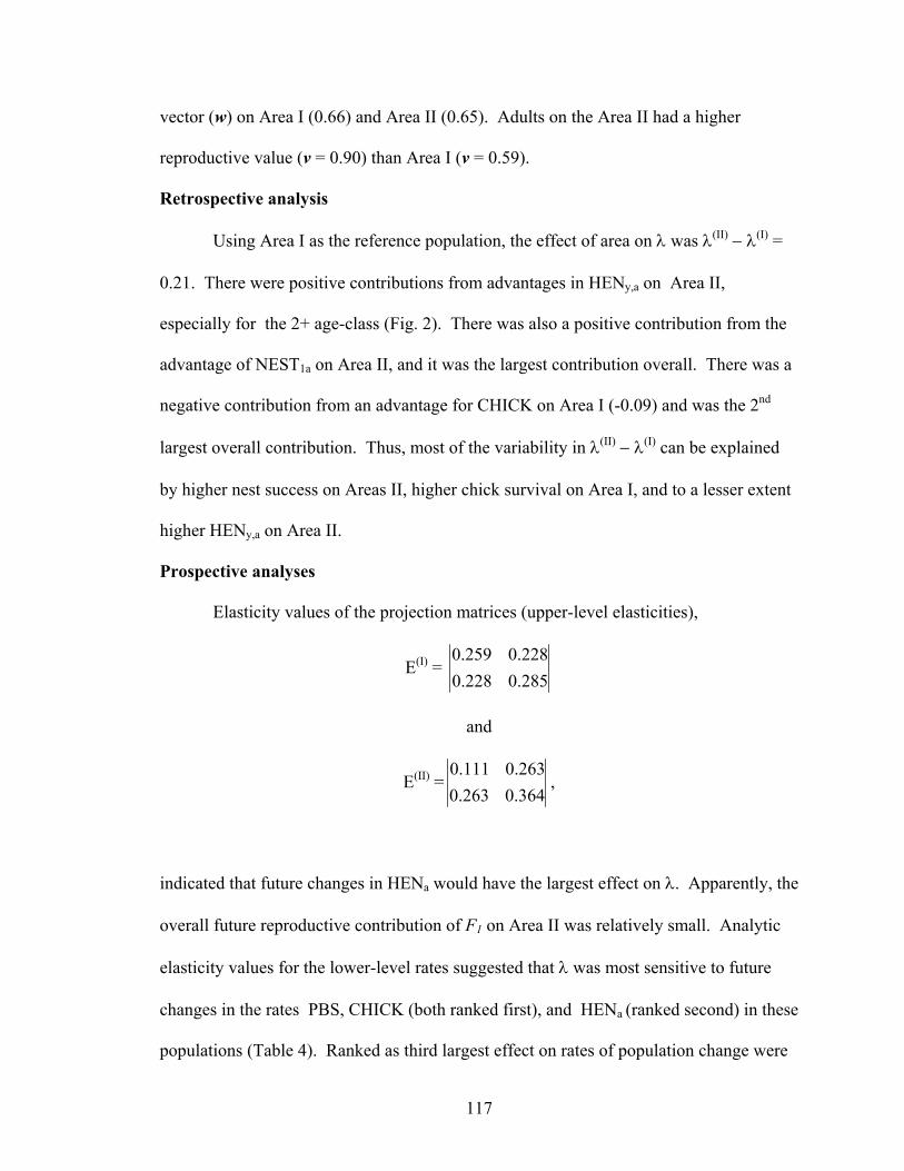
vector (w) on Area I (0.66) and Area II (0.65). Adults on the Area II had a higher

reproductive value (v = 0.90) than Area I (v = 0.59).

Retrospective analysis

Using Area I as the reference population, the effect of area on λ was λ(II) − λ(I) =

0.21. There were positive contributions from advantages in HENy,a on Area II,

especially for the 2+ age-class (Fig. 2). There was also a positive contribution from the

advantage of NEST1a on Area II, and it was the largest contribution overall. There was a

negative contribution from an advantage for CHICK on Area I (-0.09) and was the 2nd

largest overall contribution. Thus, most of the variability in λ(II) − λ(I) can be explained

by higher nest success on Areas II, higher chick survival on Area I, and to a lesser extent

higher HENy,a on Area II.

Prospective analyses

Elasticity values of the projection matrices (upper-level elasticities),

E(I) = 285.0228.0228.0259.0

and

E(II) =364.0263.0263.0111.0

,

indicated that future changes in HENa would have the largest effect on λ. Apparently, the

overall future reproductive contribution of F1 on Area II was relatively small. Analytic

elasticity values for the lower-level rates suggested that λ was most sensitive to future

changes in the rates PBS, CHICK (both ranked first), and HENa (ranked second) in these

populations (Table 4). Ranked as third largest effect on rates of population change were

117

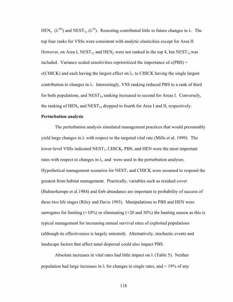
HENy (λ(II)) and NEST1y (λ(l)). Renesting contributed little to future changes in λ. The

top four ranks for VSSs were consistent with analytic elasticities except for Area II.

However, on Area I, NEST1y and HENy were not ranked in the top 4, but NEST1a was

included. Variance scaled sensitivities reprioritized the importance of e(PBS) =

e(CHICK) and each having the largest effect on λ, to CHICK having the single largest

contribution to changes in λ. Interestingly, VSS ranking reduced PBS to a rank of third

for both populations, and NEST1a ranking increased to second for Areas I. Conversely,

the ranking of HENa and NEST1a dropped to fourth for Area I and II, respectively.

Perturbation analysis

The perturbation analysis simulated management practices that would presumably

yield large changes in λ with respect to the targeted vital rate (Mills et al. 1999). The

lower-level VSSs indicated NEST1, CHICK, PBS, and HEN were the most important

rates with respect to changes in λ, and were used in the perturbation analyses.

Hypothetical management scenarios for NEST1 and CHICK were assumed to respond the

greatest from habitat management. Practically, variables such as residual cover

(Buhnerkempe et al.1984) and forb abundance are important to probability of success of

these two life stages (Riley and Davis 1993). Manipulations to PBS and HEN were

surrogates for limiting (+10%) or eliminating (+20 and 30%) the hunting season as this is

typical management for increasing annual survival rates of exploited populations

(although its effectiveness is largely untested). Alternatively, stochastic events and

landscape factors that affect natal dispersal could also impact PBS.

Absolute increases in vital rates had little impact on λ (Table 5). Neither

population had large increases in λ for changes in single rates, and < 19% of any

118

simulation had λ ≥ 1. Suggesting that relatively large changes in vital rates are required

to have any measurable effect on λ. Increases in PBS and NEST1 + CHICK had the

largest impact on both populations but neither treatment at + 30% was large enough to

maintain population stability more than 18% of the time. Future increases in PBS had the

greatest effect on λ(I) as was predicted by the elasticity values. Interestingly, the vital

rates CHICK and HEN, which had the highest rank in the VSS analysis with respect to

their effects on λ(II), responded poorly to reductions in harvest or other management

practices that might increase these survival rates. Management that simultaneously

manipulated both NEST1 + CHICK rates had far more effect on λ than did changes in

HEN.

The results of the simulated management scenarios (Table 6) complemented the

LTRE and to a lesser extent the lower-level elasticity analysis. The perturbations

indicated that λ(I) responded most to habitat management that increased NEST1 + CHICK

to 40% and relatively less to increases in PBS and HEN. However, if targeting a single

vital rate, HEN had the largest impact on λ(I). Management that simultaneously targeted

both NEST1 + CHICK rates at 40% had nearly twice effect on λ(I) (Table 6) than did

managing for HEN of 60% (66 and 100% increase of the current rates). Management

scenarios with respect to λ(II) indicated that CHICK = 40% had the largest single impact

on λ(II). HEN and PBS had a greater effect on λ(II) than did NEST1. It is not surprising

then that NEST1 + CHICK had the largest effect on λ(II).

119

DISCUSSION

Parameter estimates

This study yielded several important results about the demography of lesser

prairie-chickens and illustrated some of the more complementary sensitivity analyses

(Mills et al. 1999, Wisdom et al. 2000). I am confident of the estimates of female

survival, post-brood survival and nest success in this study, because radiomarking does

not appear to affect survival negatively (Chapter 2). High rates of censoring (> 20%) can

positively bias known-fate survival estimates when sample sizes are small (< 50 animals)

(Tsai et al. 1999). Right-censoring of adults and yearlings in this study was ~30%, and

may have biased my estimates. Alternatively, right-censoring of juvenile birds during

post-brood survival was low (6.3%) and those estimates are likely accurate, albeit from

32 birds over 3 years. Nest success in this study was similar to estimates in the literature

(Giesen 1998). Females were flushed only once during incubation to determine clutch

size. Westemeier et al. (1998) reported that flushing greater prairie chicken females from

nests resulted in 95% of those females returning to nests, and nest success was not

negatively impacted. It is possible that estimates of CHICK were biased low due to

systematic flushing; however, > 33% of all broods in this study suffered complete brood

loss prior to the first flush at 14-days post-hatch. Most flush-counts were conducted in

the morning while chicks were being “brooded” by the female, thus detection probability

was likely high. As chicks reached 34 days of age, their mobility and independence was

such that they could mix readily with other broods and it is possible that estimates of

CHICK were biased low later in the sampling period. Small sample sizes were the

greatest limitation in estimating this rate.

120

Age-structure was most prominent in survival rates when compared to the other

rates in the populations, as the transition from yearling to adult age-class was the highest

rate on both areas. This pattern of high yearling survival also occurred in banded males

during this study (Chapter 1), and reflected a life-history strategy of a “short-lived large

clutch size species” (Saether and Bakke 2000). Yearling males exhibited different

breeding behaviors in terms of site fidelity, which may have increased survival to a

second year. Similarly, yearling females may not be as tenacious in nest-defense leading

to less mortality during incubation (Chapter 3).

Projection matrix

Population assessment.—The stable age distribution (w) projected by the matrix

was similar to the actual age-structure of the radiomarked sample for both areas (yearling

= 0.38, adult = 0.62). Meeting the assumption of w in the model is important especially

when reproductive values (v) are unequal in the population (Hoekman et al. 2002), as was

the case in both of my populations. The λ’s projected 25-46% declines, but only Area I

was significantly different from λ =1. Age-ratios (0.27-0.786 yearling/adult) during

spring trapping suggests either recruitment from outside the study area or negative bias in

estimated rates of reproduction. The confidence limits around λ in both populations

suggested that in fact this rate was similar between areas. The large range of confidence

limits resulted because my parameter estimates also included sampling variance. Longer-

term studies can separate process and sampling variance and yield estimates that are more

precise. Although, the confidence bands around λ suggested no differences in these

populations, vital rates contributing to these observed values were quite different.

121

Past variability and LTRE

Population diagnosis.— LTRE has not been used previously in demographic

studies of grouse or in other conservation literature (Caswell 2001); thus comparisons

within or outside this taxon is not possible. Although a powerful tool, I was limited in

my analysis by having only 2 sites for comparisons. A larger number of study areas or an

experimental design in which one or both areas were manipulated (and pre- post-

treatment matrices were parameterized and compared) would have provided greater

resolution in the analysis.

The LTRE analysis has two important points. First, the area effect on λ was

relatively large (0.21) because fragmentation and habitat loss may have had an effect on

vital rates. These contributions were several orders of magnitude larger in the case of

NEST1 but less so for CHICK with respect to the area effect. Thus, statistically

insignificant differences in λ do not necessarily equate to equal dynamics within

populations (Caswell 1996, Johnson and Braun 1999). Second, decomposition of the

contributions to λ with respect to the lower-level rates specified the aspects of Fi that

were important to each population, CHICK, PBS, and NEST1. This provided some

insight as to why λ may not have been equal between populations. The habitat and

landscape features differed between these areas. Vegetation only differed slightly in

terms of overall sagebrush density; however Area II had 2 pastures with the highest

densities (>9,000 plants ha-1) and highest probability of nest success. Modeling of chick

survival indicated that moderate stands of sagebrush (4,000 – 6,000 plants ha-1) yielded

the highest daily survival rate (DSR) of chicks through 14-d post-hatch (Pitman 2003).

Forty percent and 10% of the pastures on Area I and II, respectively, had density

122

estimates within this range, suggesting that the elevated chick survival on Area I may

have been explained in part by the prevalence of optimal sagebrush density.

There was substantially more human disturbance (i.e., within patch

fragmentation) on Area I and may have resulted in reduced fecundity and survival

compared to Area II. Habitat fragmentation has an array of detrimental demographic

effects (Knick and Rotenberry 1995), some of which were potentially borne out in this

study. However, without the appropriate replicates, I can only discuss the implications

for these two sites. The higher density of pump-jacks, buildings, and length of road on

Area I yielded a more highly fragmented habitat (Table 1) that could have had negative

impacts on survival or reproductive output. The confounding factors of habitat structure

and landscape features will require future work to differentiate any causal relationships.

Past variation in vital rates may be important to understanding future changes to

the matrix (Wisdom et al. 1999). The LTRE in this study elucidated the vital rates in

each population that were contributing to the observed differences in λ. This suggests

that past differences in habitat or landscape may have contributed to these differences in

nest success and chick survival.

Prospective analyses (prescriptions)

Analytic perturbations.—Variance scaled sensitivities indicated that the

functional relationship of λ on CHICK was ≥ 2.1 times larger than any other rates for

Area II and nearly so (≥1.7) for Area I. I concur with the assertion of Peterson et al.

(1998) that the sensitivity to CHICK should have a greater population-level impact

because total brood loss for a female results in no contribution of young that year. Total

clutch loss of first nests may have a similar effect, but there is a probability of renesting.

123

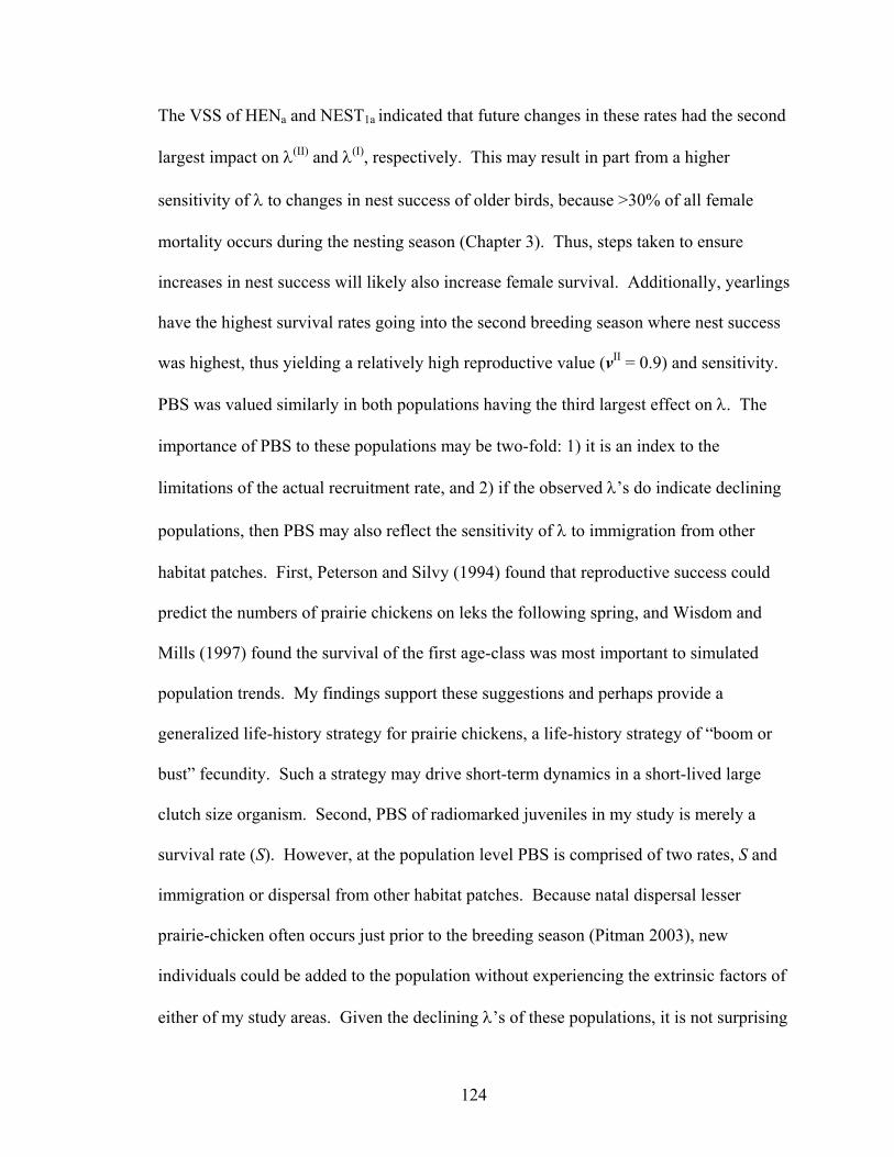
The VSS of HENa and NEST1a indicated that future changes in these rates had the second

largest impact on λ(II) and λ(I), respectively. This may result in part from a higher

sensitivity of λ to changes in nest success of older birds, because >30% of all female

mortality occurs during the nesting season (Chapter 3). Thus, steps taken to ensure

increases in nest success will likely also increase female survival. Additionally, yearlings

have the highest survival rates going into the second breeding season where nest success

was highest, thus yielding a relatively high reproductive value (vII = 0.9) and sensitivity.

PBS was valued similarly in both populations having the third largest effect on λ. The

importance of PBS to these populations may be two-fold: 1) it is an index to the

limitations of the actual recruitment rate, and 2) if the observed λ’s do indicate declining

populations, then PBS may also reflect the sensitivity of λ to immigration from other

habitat patches. First, Peterson and Silvy (1994) found that reproductive success could

predict the numbers of prairie chickens on leks the following spring, and Wisdom and

Mills (1997) found the survival of the first age-class was most important to simulated

population trends. My findings support these suggestions and perhaps provide a

generalized life-history strategy for prairie chickens, a life-history strategy of “boom or

bust” fecundity. Such a strategy may drive short-term dynamics in a short-lived large

clutch size organism. Second, PBS of radiomarked juveniles in my study is merely a

survival rate (S). However, at the population level PBS is comprised of two rates, S and

immigration or dispersal from other habitat patches. Because natal dispersal lesser

prairie-chicken often occurs just prior to the breeding season (Pitman 2003), new

individuals could be added to the population without experiencing the extrinsic factors of

either of my study areas. Given the declining λ’s of these populations, it is not surprising

124

that the vital rate that has a component somewhat independent of local constraints (and

directly adding to the population size) would be projected to have a relatively large

impact on population stability.

Comparisons to other grouse species.—Previous sensitivity analyses on 6 grouse

species have yielded mixed results (Table 7 and 8). Upper-level elasticity analyses

tended to rank survivorship of older birds higher than fecundity values (Table 7). This

was surprising for Attwater’s and greater prairie-chickens as their clutch size is markedly

larger (13 vs. 8 eggs) than that of the longer-lived greater sage-grouse and black grouse.

However, survival of juveniles to the first breeding (PBS in this study) was consistently

ranked highly among upper-level elasticities. This reiterates the importance of

recruitment both in terms of local survival and probability of immigration of the juvenile

age-class. I examined and ranked 4 lower-level elasticities that were comparable (e.g.,

nest success, chick survival, post-brood survival, and adult survival) across 4 studies

including my own (Table 8). This summary revealed that chick and PBS were generally

the first and second most important rates contributing to λ, respectively. This was

surprising given that capercaillie and willow ptarmigan have relatively small clutch sizes

compared to prairie grouse, because one would predict that λ would be most sensitive to

changes in adult survivorship in these longer-lived species.

Simulated perturbations.—Discrepancies between elasticity and perturbation

analyses was expected to some degree based on an intensive simulation study (Mills et al.

1999). Mills et al. (1999) provided evidence that infinitesimal and proportional changes

in a matrix do not reflect real changes in the environment of a species. They argue that

environmental stochasticity or management plans can potentially generate disproportional

125

and large changes in several rates simultaneously, yielding different inference about vital

rates of a population than elasticity analysis. Several studies (Mills et al.1999, Heppell et

al. 2000, Link and Doherty 2002, Nichols and Hines 2002) have concluded that elasticity

analysis was inadequate as a stand-alone result and incorporating other sensitivity indices

may yield a more complete understanding of the system. The lower-level elasticities

were weighted heavily towards adult survival and post-brood survival in this study. This

may have been due in part that the observed λ was <1 and declining populations tend be

more sensitive to adult survivorship. The perturbation analysis provided evidence in the

opposite direction indicating that nesting and brood rearing aspects of the life history

were critical to maintaining population stability for lesser prairie-chickens in southwest

Kansas. The importance of these early life stages was echoed in the LTRE as mentioned

above. Thus, increases in adult survivorship or post-brood survival by eliminating

hunting (<5% of all current mortality) would do little to stabilize these populations.

However, hunting of a declining population can only be justified if it is compensatory to

annual survival. This was contrary to the findings of Steen and Erikstad (1996) and

Johnson and Braun (1999); both studies found that decreases in adult survivorship from

hunting negatively affected population growth, especially in years with poor recruitment.

However, the markedly higher harvest rates in those studies likely had a larger effect on

survival than that observed in my study.

Conclusions

Population prognosis.— Ascertaining the status of these populations was difficult

given that both sampling and process variance were included in the parameter estimates.

However, efforts to increase nesting success and chick survival are paramount, and the

126

former likely will increase female survival. The tenuous stability of λ in these two

populations suggests that these fragmented populations are maintained in part by

immigration. Lek survey routes through this region have not detected the declines

reported here (KDWP unpublished data), and age-ratio data collected during this study

support the idea that immigration is a potential mechanism for population stability. It is

noteworthy that the results of this comprehensive field study reflected the conclusions of

other workers on prairie grouse (Peterson and Silvy 1994, Wisdom and Mills 1997,

Peterson et al. 1998) that extracted rates from the literature and across large geographical

regions. It is clear from this study and other modeling exercises (Wisdom and Mills

1997, Peterson et al. 1998) on prairie grouse that nesting and brood rearing are the critical

rates to maintaining population stability. This study also indicated the importance of

immigration via post-brood survival from other habitat patches. Management efforts

aimed at increasing the quality, and/or quantity of nesting and brood habitat will have the

greatest benefits to lesser prairie-chicken populations. Alternatively, this study provided

some initial insight as to the impacts of hunting on a declining species, and indicated that

eliminating hunting (if additive) would not yield a stable population.

ACKNOWLEDGMENTS


Beach for property access. I thank J. C. Pitman for sharing his unpublished data on nest

success and chick survival, C. G. Griffin, B. E. Jamison, J. C. Pitman ,G. C. Salter, T. L.

Walker, Jr., and T. J. Whyte for assistance with field work. B. K. Sandercock provided

assistance with computer programming and advice on developing the matrix models.

Financial and logistical support was provided by Kansas Department of Wildlife and

127

Parks (Federal Aid in Wildlife restoration projects, W-47-R and W-53-R), Kansas

Agricultural Experiment Station (Contribution No. 03-_______), Division of Biology at

Kansas State University, and Westsar Energy Inc.

LITERATURE CITED Amman, G. A. 1944. Determining the age of pinnated and sharp-tailed grouse. Journal of



A. T. Bergerud and M. W. Gratson, editors. Adaptive Strategies and Population

Ecology of Northern Grouse. Wildlife Management Institute, Washington DC,

USA.

Blakesly, J. A., B. R. Noon, and D. H. Shaw. 2001. Demography of the California

spotted owl in northeastern California. Condor 103.

Buhnerkempe, J. E., W. R. Edwards, D. R. Vance, and R. L. Westemeier. 1984. Effects

of residual vegetation on prairie-chicken nest placement and success. Wildlife

Society Bulletin 12: 382-386.

Caizerigues, A., and L. N. Ellison. 1997. Survival of black grouse Tetrao tetrix the

French Alps. Wildlife Biology 3: 177-186.

Caswell, H. 1996. Analysis of life table response experiment II. alternative

parameterization for size and stage structured models. Ecological Modelling 88:

73-82.

Caswell, H. 2001. Matrix population models. Sinauer, Sunderland, Massachusetts.



USA.

Cottam, G., and J. T. Curtis. 1956. The use of distance measures in phytosociological

sampling. Ecology 37: 451-460.

128

Crouse, D. T., L. B. Crowder, and H. Caswell. 1987. A stage-based population model for

loggerhead sea turtles and implications for conservation. Ecology 58: 1412-1423.

Ebert, T. A. 1999. Plant and animal populations: methods in demography. Academic

Press. San Fransico, California.

Fieberg, J., and S. P. Ellner. 2001. Stochastic matrix models for conservation and

management: a comparative review of methods. Ecology Letters 4.

Flint, P. L., K. H. Pollock, D. Thomas, and J. S. Sedinger. 1995. Estimating prefledging

survival: allowing for brood mixing and dependence among brood mates. Journal

of Wildlife Management448-455.

Giesen, K. M. 1998. Lesser Prairie-Chicken (Tymapanuchus pallidinctus). in The Birds

of North America. No. 364. (F. Gill and A. Poole, editors) The Birds of North

America Inc., Philadelphia, Pennsylvania, USA.

Grimm, V., and I. Storch. 2000. Minimum viable population size of capercaillie Tetrao

urogallus: results from a stochastic model. Wildlife Biology 6: 219-225.



Heppell, S. S., H. Caswell, and L. B. Crowder. 2000. Life histories and elasticity

patterns: perturbation analysis for species with minimal demographic data.

Ecology 81: 654-655.

Hoekman, S. T., L. S. Mills, D. W. Howerter, J. H. Devries, and I. J. Ball. 2002.

Sensitivity analyses of the life cycle of midcontinent mallards. Journal of Wildlife





129




Johnson, K. H., and C. E. Braun. 1998. Viability and conservation of an exploited sage

grouse population. Conservation Biology 13: 77-84.

Knick, S. T., and J. T. Rotenberry. 1995. Landscape characteristics of fragmented

shrubsteppe habitats and breeding passerine birds. Conservation Biology 9: 1059-

1071.

Link, W. A., and P. F. Doherty, Jr. 2002. Scaling sensitivity analysis. Ecology 83: 3299-

3305.

Manly, B. F. 1991. Randomization, bootstrap and Monte Carlo methods in biology. Chapman &

Hall. London, England, UK.

Mills, L. S., D. F. Doak, and M. J. Wisdom. 1999. Reliability of conservation actions

based on elasticity analysis of matrix models. Conservation Biology 13: 815-829.

Nichols, J. D., and J. E. Hines. 2002. Approaches for the direct estimation of λ and

demographic contributions to λ using capture-recapture data. Journal of Applied

Statistics 29: 539-568.

Peterson, M. J., W. T. Grant, and N. J. Silvy. 1998. Simulation of reproductive stages

limiting productivity of the endangered Attwater's prairie-chicken. Ecological

Modelling 111: 283-295.

Peterson, M. J., and N. J. Silvy. 1996. Reproductive stages limiting productivity of the

endangered Attwater's prairie-chicken. Conservation Biology 4: 1264-1276.

Pitman, J. C. 2003. Lesser prairie-chicken nest site selection and nest success, juvenile

gender determination and growth, and juvenile survival and dispersal in

southwestern Kansas. Thesis, Kansas State University, Manhattan, Kansas.

130

Riley, T. Z., and C. A. Davis. 1993. Vegetative characteristics of lesser prairie-chicken

brood foraging sites. Prairie Naturalist 25: 243-248.

Saether, B. E., and O. Bakke. 2000. Avian life history variation in contribution of

demographic traits to the population growth rate. Ecology 81: 642-653.

Schroeder, M. A. and L. A. Robb. 1993. Greater prairie-chicken (Tympanuchus cupido).

in The Birds of North America No. 36. (A. Poole, P. Stettenheim, and F. Gill,

editors) The Birds of North America, Inc., Philadelphia, Pennsylvania, USA.

Steen, H., and K. E. Erikstad. 1996. Sensitivity of willow grouse Lagopus lagopus

population dynamics to variations in demographic parameters. Wildlife Biology

2: 27-35.

Temple, S. A. 1992. Population viability analysis of sharp-tailed grouse metapopulation

in Wisconsin. Wildlife 2001: Populations, 750-758.

Tsai, K., K. H. Pollock, and C. Brownie. 1999. Effects of violation of assumptions for

survival analysis methods in radiotelemetry studies. Journal of Wildlife



threatened wildlife and plants; review of species that are candidates and proposed

for listing as endangered or threatened: the lesser prairie-chicken . Federal

Register 67: 40667.


Game Magazine1-4.

Westemeier, R. L., J. E. Buhnerkempe, and J. D. Brawn. 1998. Effects of flushing

nesting greater prairie-chickens in Illinois. Wilson Bulletin 110: 190-197.



131

Wisdom, M. J., and L. S. Mills. 1998. Sensitivity analysis to guide population recovery:

prairie-chicken as an example. Journal of Wildlife Management 61: 302-312.

Wisdom, M. J., L. S. Mills, and D. F. Doak. 2000. Life stage simulation analysis:

estimating vital-rate effects on population growth for conservation. Ecology 83:

628-641.



Marzluff, editors. Radio Tracking and Animal Populations. Academic Press, San

Diego, California, USA.

132

Table 1. Habitat and landscape features for study areas I and II in southwestern Kansas,

1998-2003. Parameter and standard errors (in parentheses) presented when a variable

was not directly measured.

Habitat feature Area I Area II

Fragment size (ha) 5,684 5,660

Sagebrush density (ha-1) 3,611 (689) 4,206 (697)

Sagebrush height (cm)

57 (5.7) 55 (5.9)

Sagebrush diameter (cm) 76 (9.9) 66 (12.5)

Road (km) 154.7 129.2

Powerline (km) 28.4 30.8

Pump-jack (ha-1,000) 10.6 6.9

Buildings (n) 6 1

133

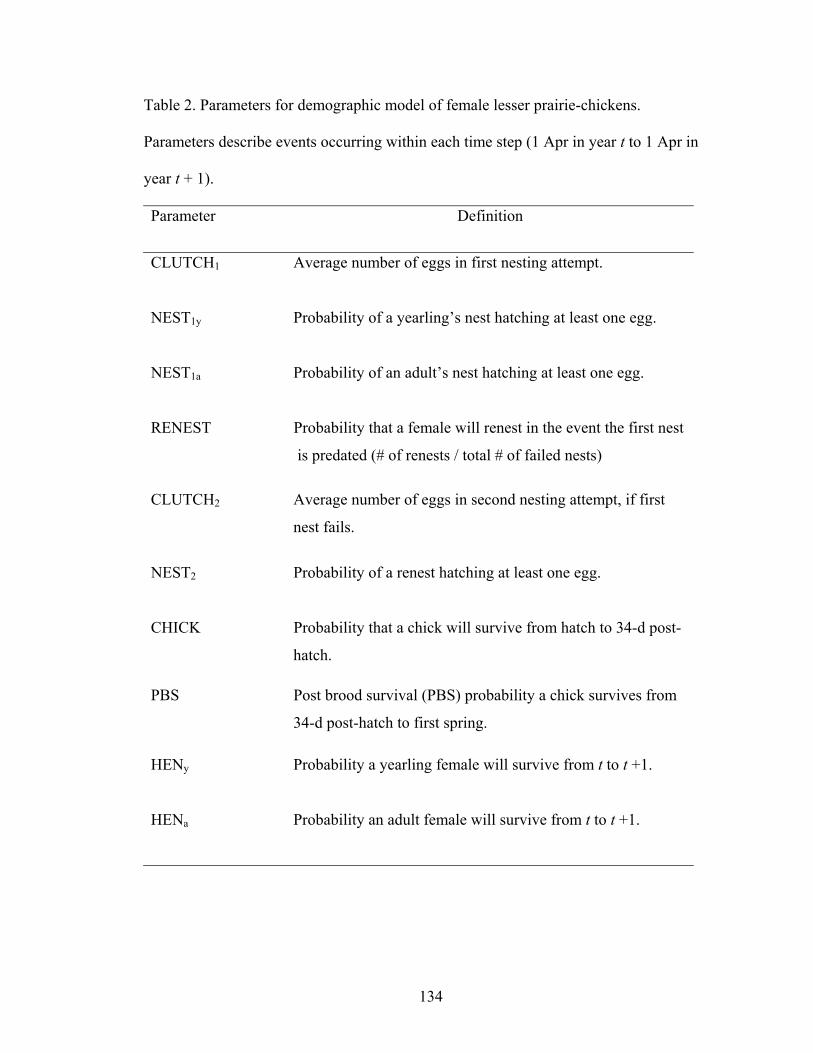
Table 2. Parameters for demographic model of female lesser prairie-chickens.

Parameters describe events occurring within each time step (1 Apr in year t to 1 Apr in

year t + 1).

Parameter Definition

CLUTCH1 Average number of eggs in first nesting attempt.

NEST1y Probability of a yearling’s nest hatching at least one egg.

NEST1a Probability of an adult’s nest hatching at least one egg.

RENEST Probability that a female will renest in the event the first nest

is predated (# of renests / total # of failed nests)

CLUTCH2 Average number of eggs in second nesting attempt, if first

nest fails.

NEST2 Probability of a renest hatching at least one egg.

CHICK Probability that a chick will survive from hatch to 34-d post-

hatch.

PBS Post brood survival (PBS) probability a chick survives from

34-d post-hatch to first spring.

HENy Probability a yearling female will survive from t to t +1.

HENa Probability an adult female will survive from t to t +1.

134

Tabl

e 3.

Par

amet

er e

stim

ates

(θ) o

f vita

l rat

es o

f yea

rling

(Y) a

nd a

dult

(A) l

esse

r pra

irie-

chic

kens

radi

o-m

arke

d in

Fin

ney

Cou

nty,

Kan

sas 1

998-

2002

. Vita

l rat

es a

re d

efin

ed in

Tab

le 2

.

Are

aI

Are

aII

Vita

l rat

e Y

θ ±

SEa

A

θ ±

SE

Y

θ ±

SE

A

θ ±

SE

Pool

ed

θ ±

SE

NES

T 1b

0.30

3 ±

0.08

0 (3

3)c

0.14

0 ±

0.05

3 (4

3)

0.

320 ±

0.09

3 (2

5)

0.41

5 ±

0.07

7 (4

1)

--

NES

T 2

0.14

3 ±

0.16

3 (1

4)

0.12

5 ±

0.08

0 (1

6)

--

REN

EST

0.22

3 ±

0.05

5 (6

0)

0.41

0 ±

0.07

9 (3

9)

--

C

LUTC

H1

----

----

12.1

± 1

.6 (1

51)

CLU

TCH

2--

----

--7.

7 ±

3.0

(29)

CH

ICK

0.

293 ±

0.13

1 (1

2)

0.

209 ±

0.08

0 (2

6)

--

PBSc

----

----

0.53

9 ±

0.08

9 (3

2)

HEN

0.

429 ±

0.11

7 (2

4)

0.30

2 ±

0.08

0 (5

0)

0.

588 ±

0.10

0 (3

3)

0.43

8 ±

0.08

3 (4

8)

--

135

a Clu

tch

size

s wer

e re

porte

d w

ith ±

1 st

anda

rd d

evia

tion,

all

prob

abili

ties w

ith ±

1 st

anda

rd e

rror

, and

sam

ple

size

s are

in p

aren

thes

es.

b All

para

met

er e

stim

ates

exc

ept f

or h

en su

rviv

al w

ere

calc

ulat

ed fr

om fi

eld

data

gat

here

d be

twee

n 19

98 a

nd 2

002.

Ann

ual h

en

surv

ival

was

onl

y es

timat

ed fr

om 2

000

to 2

003.

c Th

e es

timat

es o

f clu

tch

size

s (C

LUTC

H1,

2) a

nd p

ost-b

rood

surv

ival

(PB

S) w

ere

pool

ed a

cros

s are

as a

nd a

ge-c

lass

es d

ue to

con

stan

cy

of ra

tes,

and

sam

ple

size

s, re

spec

tivel

y.

Table 4. Analytic elasticities and variance scaled (arc-sin) sensitivities (VSS) for lower-

level vital rates of matrix.

Area I Area II

Vital ratea Elasticity VSS Elasticity VSS

NEST1y 0.24 0.37 0.10 0.15

NEST1a 0.20 0.49 0.24 0.29

RENEST 0.05 0.11 0.03 0.08

NEST2 0.05 0.09 0.03 0.04

CHICK 0.49 0.76 0.37 0.73

PBS 0.49 0.45 0.37 0.35

HENy 0.23 0.26 0.26 0.22

HENa 0.29 0.43 0.36 0.41

a Vital rates defined in Table 2.

136

Table 5. Results of a life stage simulation analysis (LSA) in which each vital rate was

increased by 10, 20, and 30 % (of its current estimate) and its variability decreased by

10%. The proportion of simulated matrices (n = 1,000) for each vital rate and percent

increase that resulted in λ ≥ 1, is a measure of management effectiveness.

Vital rates (Proportion of 1,000 simulations where λ ≥ 1)

Area / rate increase

NEST CHICK NEST + CHICK

PBS HEN

Area I

10% 0.009 0.007 0.014 0.082 0.010

20% 0.018 0.010 0.032 0.127 0.005

30% 0.027 0.015 0.059 0.180 0.007

Area II

10% 0.026 0.037 0.048 0.062 0.029

20% 0.037 0.066 0.072 0.116 0.057

30% 0.059 0.079 0.133 0.174 0.082

137

Table 6. Results of a modified LSA in which each vital rate was targeted for a set rate of

30 and 40% for nesting and chick survival, and 50 and 60% for post-brood survival and

female survival. Variability was simultaneously decreased by ~20% for each rate. The

proportion of simulated matrices (n = 1,000) for each vital rate and it management goal

that resulted in λ ≥ 1, is a measure of management effectiveness.

Vital rates (Proportion of 1,000 simulations where λ ≥ 1)

Area / targeted rate

NEST CHICK NEST + CHICK

PBS HEN

Area I

30 (20-40)% 0.009 0.000 0.001 NDa ND

40 (30-50)% 0.059 0.005 0.140 ND ND

50 (40-50)% ND ND ND 0.015 0.035

60 (50-70)% ND ND ND 0.036 0.089

Area II

30 (20-40)% 0.004 0.098 0.029 ND ND

40 (30-50)% 0.032 0.286 0.365 ND ND

50 (40-50)% ND ND ND 0.015 0.041

60 (50-70)% ND ND ND 0.077 0.081

a ND = no data recorded for these simulations.

138

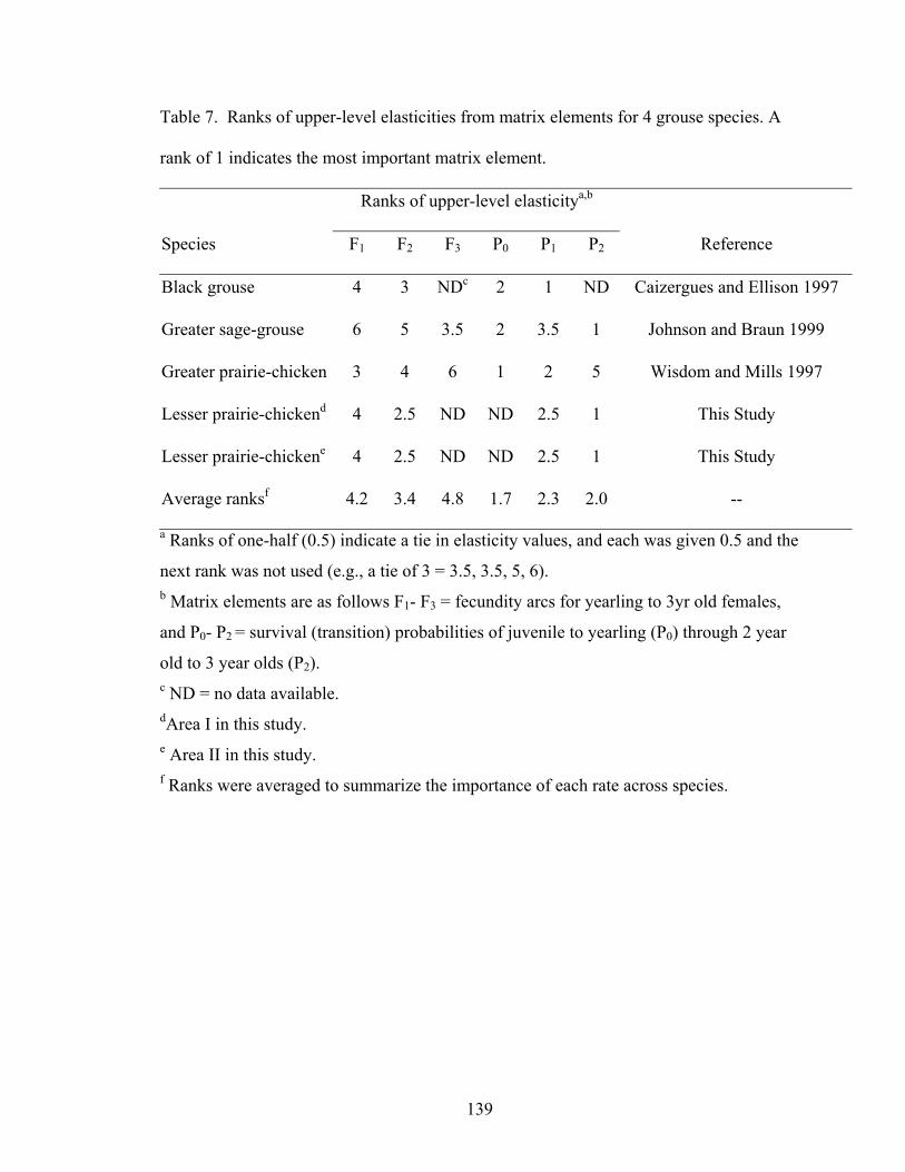
Table 7. Ranks of upper-level elasticities from matrix elements for 4 grouse species. A

rank of 1 indicates the most important matrix element.

Ranks of upper-level elasticitya,b

Species F1 F2 F3 P0 P1 P2 Reference

Black grouse 4 3 NDc 2 1 ND Caizergues and Ellison 1997

Greater sage-grouse 6 5 3.5 2 3.5 1 Johnson and Braun 1999

Greater prairie-chicken 3 4 6 1 2 5 Wisdom and Mills 1997

Lesser prairie-chickend 4 2.5 ND ND 2.5 1 This Study

Lesser prairie-chickene 4 2.5 ND ND 2.5 1 This Study

Average ranksf 4.2 3.4 4.8 1.7 2.3 2.0 --

a Ranks of one-half (0.5) indicate a tie in elasticity values, and each was given 0.5 and the

next rank was not used (e.g., a tie of 3 = 3.5, 3.5, 5, 6). b Matrix elements are as follows F1- F3 = fecundity arcs for yearling to 3yr old females,

and P0- P2 = survival (transition) probabilities of juvenile to yearling (P0) through 2 year

old to 3 year olds (P2). c ND = no data available. dArea I in this study. e Area II in this study. f Ranks were averaged to summarize the importance of each rate across species.

139

Table 8. Ranks of lower-level elasticities from matrix elements for 4 grouse species. A

rank of 1 indicates the most important vital rate.

Lower-level elasticity ranksa

Nest

success PBS Adult Reference

Willow ptarmigan 5 4 1 2.5 Steen and Erikstad 1996

Attwaters prairie-chicken 3 1 4 2 Peterson et al. 1998

Capercaillie 3 1 NDe 2 Grimm and Storch (2000)

Lesser prairie-chickenb 3.5 1 3 5 This Study

Lesser prairie-chickenc 5 1 3 3.5 This Study

Average ranksd 3.9 1.6 2.8 3 --

Chick

a Ranks of one-half (0.5) indicate a tie in elasticity values, and each was given 0.5 and the

next rank was not used (e.g., a tie of 3 = 3.5, 3.5, 5, 6). b Area I in this study. c Area II in this study. d Ranks were averaged to summarize the importance of each rate across species. e ND = no data available.

140

Fig. 1. Life-cycle diagram and matrix for a 2 age-class pre-breeding model of female

lesser prairie-chickens. Notations for vital rates are defined in the text.

141

=

1

201

PPFPF

A

F2

F1 P1

P2 Y

142

A

2

0P

Fig. 2. Results of the life-table response experiment (LTRE) show the contribution of

each vital rate to the difference in λ between Area I (lower half of panel) and Area II

(upper half of panel). This retrospective analysis determined that advantages of NEST1a

and CHICK on Area II and I, respectively, had the largest contribution to population

growth. Notations for vital rates are defined in the text.

143

NEST1y NEST1a RENEST NEST2 CHICK HENy HENa

Con

tribu

tion

to λ

Ι - λΙΙ

= 0

.21

-0.10

-0.05

0.00

0.05

0.10

0.15

144

CHAPTER 5

THE EFFECTS OF LANDSCAPE FEATURES ON LESSER PRAIRIE-CHICKEN

HABITAT USE

Abstract: Suitable habitat for the lesser prairie-chicken (Tympanuchus pallidicinctus) has

been reduced markedly over the past 100 years. The remaining habitat is widely used for

petroleum exploration and extraction, cattle grazing, powerline easements, and the

generation of electricity. Given the tenuous status of the species and the demands on land

use for its remaining habitat, it is imperative that suitable habitat be quantified for impact

assessment and conservation planning. I examined the relationship of several habitat

characteristics and landscape features as they pertained to habitat suitability in

southwestern Kansas. I quantified these characteristics in use and non-use areas as

determined from the presence or absence of prairie chicken locations determined by

radiotelemetry data from 1997 to 1999. I extended the analysis and quantified the

proportion of landscape features and sagebrush density in monthly-ranges of radiomarked

birds 2000 to 2002. The MANOVA results indicated habitat selection by prairie

chickens. Canonical variates analysis resulted in 87 and 13% of the data explained by

canonical variates-1 and -2, respectively. Canonical variate-1 was positively correlated

with sagebrush density, cover, and diameter, but negatively correlated with distance to

wells and structures. This linear combination best described absent-sites. Canonical

variate-2 had the strongest positive correlation with distance to powerline, and best

described use-sites. The average odds of a powerline occurring in a non-range were 3.22

times more likely than in a monthly-range. Monte Carlo simulations of distances to

145

structures indicated that the nearest 40% of lesser prairie-chicken centers of use were

farther from anthropogenic features than would be expected at random.

INTRODUCTION

Suitable habitat for the lesser prairie-chicken (Tympanuchus pallidicinctus) has

been markedly reduced over the past 100 years. What remains is highly fragmented

throughout the species’ range (Giesen 1998). The remaining habitat is widely used for

petroleum exploration and extraction, cattle grazing, powerline easements, and the

generation of electricity (Jamison et al. 2001a). The cumulative loss of habitat and

declining population trends led to the “warranted but precluded” threatened listing under

the Endangered Species Act (USFWS 2002). The lesser prairie-chicken’s dependency on

native rangeland has been well studied, at the microscale (Jones 1963, Crawford and

Bolen 1974, Riley et al. 1992, Jamison et al. 2001b), and the macroscale (Jamison 2000,

Woodward et al. 2001, Fuhlendorf et al. 2002). Despite these large-scale contractions of

habitat and thorough examination of microhabitat variables, little is known about the

specific parameters of a suitable habitat patch. Given the tenuous status of the species

and the demands on land use for its remaining habitat, it is imperative that suitable habitat

be quantified for conservation assessment and planning.

Jamison (2000) examined habitat use of male lesser prairie-chickens as it

pertained to selection ratios of sand sagebrush (Artemisia filifolia), cropland, and

miscellaneous grasslands in southwestern Kansas. Generally, lesser prairie-chickens

were tied to sagebrush throughout the year, but exhibited higher selection ratios for this

cover-type during the summer months (Jamison 2000). Despite the apparent importance

of sagebrush, there were several areas within the prairie fragment (~5,000 ha) in which

146

radiomarked birds were not located, and unmarked individuals were not flushed or

observed in these areas (B. E. Jamison, unpublished data). This lack of habitat use

provided an opportunity to quantify both habitat variables and landscape features as they

pertain to suitability of lesser prairie-chicken habitat.

The objective of this paper is to examine what suite of habitat characteristics and

landscape features determines habitat suitability in southwestern Kansas. I used

Jamison’s (2000) radiotelemetry location data of male and female lesser prairie-chickens

to quantify these characteristics in use and non-use sites as determined from the presence

or absence of prairie chicken locations. I extended the analysis in 2000-2002 and

quantified the proportion of landscape features and sagebrush density in monthly-ranges

of radiomarked females.

METHODS

Study area

The study region was comprised of 2 fragments (~5000 ha each) of native

sandsage prairie near Garden City, Finney County, Kansas (37° 52′ N, 100° 59′ W).

Work began on Area I (southwest of Garden City) in 1997. In 2000, trapping and

monitoring efforts were expanded to include Area II (southeast of Garden City). Prior to

1970, these 2 areas were part of a contiguous tract of native sandsage prairie. The

development of center pivot irrigation left these areas as two fragments with about 19 km

of non-habitat between patch centroids (Waddell and Hanzlick 1978). Shrub and grass

vegetation in the prairie fragments was comprised of sandsage, yucca (Yucca spp.),

sandreed grasses (Calamovilfa spp.), bluestem grasses, sand dropseed (Sporobolus

cryptandrus), and sand lovegrass (Eragrostis trichodes). Primary forb species in the

147

region included ragweed (Ambrosia spp.), sunflower (Helianthus spp.), and Russian

thistle (Salsola iberica) (Hullett et al. 1988, Jamison 2000).

Field methods

Lesser prairie-chickens were captured on leks using walk-in funnel traps during

March and April 1997-2002 (Haukos et al. 1991). Each captured bird was fitted with a

lithium battery powered transmitter with a mass < 12-g. During Phase I (1997–1999)

males and females were tracked daily from April to September 1997, and April to April

1998–2000. Females were tracked daily from April to April during Phase II (2000-

2003). A truck-mounted null-peak twin-Yagi telemetry system was used to triangulate

individuals remotely.

Retrospective analysis (Phase I)

Defining use.–I quantified both micro- and macrohabitat variables that occurred in

use and non-use areas as determined from Jamison’s (2000) study from 1997 to 1999.

Thus, I sampled vegetation in the areas defined below in 2000 and 2001. Use areas were

defined from a 95% fixed kernel home range (Worton 1989) of all lesser prairie-chicken

locations (n = 21,363) that intersected the study area (Jamison 2000). Areas not

intersected by this polygon were defined as non-use areas. I defined 2 types of non-use

sites: 1) areas adjacent to use sites but where radiomarked birds were never located

(hereafter non-use sites), and 2) an area north of the Sunflower Electric Power plant

(Area I southwest of Garden City, KS) which was not known to have breeding

populations of prairie chickens, and where radiomarked birds were never located

(hereafter absent sites). Although I cannot make absolute statements regarding the

148

avoidance of these areas by lesser prairie-chickens, the data recorded over 6 years never

documented radiomarked or unmarked birds in absent and non-use areas.

Sampling.–I generated random points (UTM coordinates) within use-, non-use,

and absent areas in ARCVIEW 3.1 (ESRI 1998). Random points were located in the

field using a handheld global positioning system (GPS) unit. At each random point, I

placed a 1.5 × 0.5 m quadrat and estimated the percent cover of shrub, grass, forb, and

litter. Shrub density ha-1 was estimated using a modification of the point center quarter

method (Cottam and Curtis 1956), where if the nearest shrub was > 15 m from the

random point that quadrant was censored, and density was estimated based upon both the

number of distances measured and the number censored (T. Loughin, Kansas State

University, unpublished data). This modification was necessary to increase the efficiency

of data collection in the field. Distances to the nearest road, powerline, natural gas or oil

well-head (hereafter wells), and structure (e.g., dwellings, compressor station, ash-pile or

powerplant) from each random point were calculated in a geographic information system

(GIS).

Home range estimation and GIS (Phase II)

For the location data from 2000 to 2002 the analyses were extended and

quantified the proportion of landscape features and sagebrush density in monthly-ranges

of radiomarked females. Azimuths from fixed listening stations were entered into Locate

II triangulation software (Nams 2002), and locations of prairie chickens were estimated

using Lenth maximum likelihood estimators. Location data were imported into a GIS

database of the study area and monthly ranges were estimated using a 95% fixed kernel

(Worton 1989) in ARCVIEW 3.1. I limited my sample to those birds that had ≥20

149

locations per month. While this reduced the number of observational units, it ensured

that observed range sizes were likely representative of the area covered in a month

relative to birds with fewer locations. This also limited the season for which such an

analysis could be conducted as the season progressed the number of individuals tracked

decreased and premature battery failure also contributed to reductions in sample size.

Thus, I chose to focus the analysis on times of the year (April to September) when

samples were relatively large and coincided with a peak usage of sagebrush habitats

(Jamison 2000). All female locations that occurred on nest sites were excluded as the

relationship between nesting and these variables has already been examined (Pitman

2003).

Locations of wells, roads, powerlines, and structures were digitized into the GIS.

Monthly ranges for each bird were computed separately for year and month (e.g., Apr

2000) to control for yearly and biological variation in monthly habitat use. The ranges

for all birds in a given year and month were combined into a single overall “use range”

which was overlaid onto the study area. Each year and month layer (hereafter a

monthly-range) was used as a sampling frame to calculate the number of wells, roads,

powerlines and structures falling within and outside of (hereafter non-ranges) prairie

chicken monthly-ranges. Wells could be counted directly, however, roads and

powerlines could not. Thus, following the procedure of Marcum and Loftsgaarden

(1980) 244,000 random points were generated within each of the study area polygons and

the number of points that intersected roads and powerlines in use and non-use areas

tabulated. This resulted in count-data that could be input into contingency table or

Poisson rate regression analyses.

150

Analysis

Retrospective analysis of use.—A fixed model MANOVA (PROC GLM: SAS)

was used to examine habitat use for a community of variables (Johnson 1998). This

model allowed me to compare the effect of habitat characteristics and landscape features

on use simultaneously. I used MANOVA as a conservative approach to multiple

comparisons, and to examine the dimensionality of the alternative hypothesis using

canonical variates analysis (Johnson 1998). Thus, I reported the means and standard

errors of habitat and landscape variables, and their resulting P-values from multiple

comparisons. I examined the possibility of explaining these sites in a reduced parameter

space (i.e. the dimensionality of the alternative hypothesis). The dimensionality of Ho =

3, and Ha < 3 in this study. If the population means lie in a subspace (data reduction)

then linear combinations (canonical variates) can be used to explain the relationship

between use, non-use, and absent sites. I tested the differences in mean canonical

variates using differences of means and 95% confidence limits around the differences,

and the degree of overlap of 95% ellipses in a 2-dimensional space (canonical variate-1 ×

canonical variate-2). The approximate 95% ellipses were estimated as

nk

2,αχ

,

where χ2 = chi-square value at α = 0.05, k = number of dimensions, n = number of

populations, and if k = 2 then the ellipses are circles.

Six habitat variables were included in analyzing use, non-use, and absent sites:

percent cover estimates for sagebrush, grass, forb, and litter; shrub density, and shrub

diameter. Distances from random points (within the areas defined above) to the nearest

151

structure, well, powerline, and road (included both paved and unimproved trails) were

also included in the analysis.

Monthly-ranges and use.—In the following analyses it is important to recognize

that monthly usage included repeated measures on individual birds. This limits my

inference and may increase my Type I error rate if certain individuals had a propensity to

remain farther from these features than the population mean. However, only 60% of the

birds had consistent repeated measures through the sampling period, making a repeated

measures design impractical. Thus, I treated monthly-range as the observational unit and

blocked on month. Because the goal of the analysis is not to differentiate the variation in

usage across months but to examine general patterns of use as it pertains to these

landscape features, I assessed the effects on use and controlled for the monthly

variability by blocking on month.

I used 2 × 2 × K contingency tables and Poisson rate regression to examine the

relationships between monthly-ranges and the proportion of each area occupied by

powerlines, roads, and wells controlling for months there were 6 blocks in 2000 and

2001, and 4 blocks in 2002. Contingency tables were used to examine the proportion of

roads and powerlines present in monthly-ranges compared to non-range areas. The

Breslow-Day test for homogeneity of odds ratios was used to test for a common odds

ratios across months (Agresti 1996). Poisson rate regression was used to model the

number of wells present in monthly-ranges as a function of use month and year.

Backward selection was used to find the most parsimonious model that fit well, and

model fit was assessed by examining the scale parameter (deviance / df) and residual

plots.

152

Sagebrush density was estimated for monthly- and non-ranges of lesser prairie-

chickens using the modification of the point-center quarter (PCQ) method described

above. Density was estimated from a database of >3,000 points where PCQ

measurements were taken. I tested for the effect of use on differences in density between

ranges using a mixed model ANOVA, blocking on month.

Permutations of structure distance.—Because structures were not randomly or

uniformly located on the landscape in relation to monthly-ranges, I used a modified

Monte Carlo simulation (Manly 1997) to test whether the centroids of monthly-ranges

were farther from structures than would be expected at random. If the structures had no

impact on the birds' monthly-ranges, then one would expect the distances between these

centroids and the structures to follow the same distribution as distances to randomly-

placed points. If, on the other hand, the birds demonstrated some avoidance of these

structures, as hypothesized, then the centroids closest to these structures should tend to be

farther away than the random points. I therefore compared the 5th, 10th, 20th, 30th and 40th

percentiles of the observed distances to the respective distributions of the correcponding

percentiles from randomly-placed points as follows: 1) random resamples of 81 distances

were taken from the distribution of 100,000 random points and distances; 2) this was

repeated 1,000 times (thus generating 1,000 resamples of 81 distances); 3) the 5th, 10th,

20th, 30th and 40th percentiles for each resample were calculated; 4) an estimated sampling

distribution of each percentile was created based on the 1000 calculated percentiles; and

5) the observed percentile distances were compared to the the upper tail of their

respective sampling distribution. If the observed percentile distance was too extreme in

the upper tail (i.e. in the upper 5% of the distribution), the Ho (structures do not affect

153

monthly-range placements) was rejected. Support for the Ha, that structures have a

negative impact on habitat use was then examined. The observed percentiles and the

expected (mean) value of that percentile under randomness were compared.

RESULTS

Use and non-use

A total of 281 lesser prairie-chickens were captured and 160 (male = 76, female =

84) were fitted with transmitters. This resulted in 21,373 daily locations from 1997 to

1999. Vegetation sampling points in use (n = 44), non-use (n = 38), and absent (n = 46)

areas were also used to calculate distances to landscape features. The MANOVA results

indicated habitat selection by prairie chickens (Wilks Λ = 0.352, F20,222 = 7.58, P <

0.0001) with large numbers of multiple comparisons with effect sizes 1- to 2-fold

differences between means (Table 1). The dimensionality of Ha = 2 (canonical variate-

1, F20,222 = 7.58, P < 0.0001; canonical variate-2, F9,112 = 2.48, P = 0.013) and canonical

variates-1 and -2 (CAN-1 and CAN-2) explained 87 and 13% of the data, respectively.

Canonical variate-1 was positively correlated with sagebrush density, cover, and diameter

(Table 1), but negatively correlated with distance to wells and structures; collectively this

describes absent-sites. Canonical variate-2 had the strongest positive correlation with

distance to powerline, and use-sites (Table 2). Thus, lesser prairie-chicken habitat use

was generalized by the linear combinations, CAN-1 and CAN-2, of sagebrush stand

characteristics and well proximity, and distance to powerlines, respectively. Effect sizes

and 95% confidence intervals of the mean CAN-1 scores (Table 2) for use, non-use, and

absent areas indicated that differences in shrub habitat were similar between use and non-

use sites ( usenonuse xx −− = 0.365, 95% CI: -0.070, 0.800), but differed markedly from

154

absent sites ( usenonabsent xx −− = 2.621, 95% CI: 2.183, 3.059; useabsent xx − = 2.256, 95% CI:

1.816, 2.696). This was supported by sagebrush density estimates obtained from

calculations of all sampling points within each area. Densities were: absent = 7, 205 SE

= 573; non-use = 2,553 SE = 201; and use sites = 3,144 SE = 249 ha-1. Conversely,

CAN-2 scores revealed (Table 2) greater similarity between non-use and absent sites in

terms of distance to landscape features ( usenonabsent xx −− = 0.403, 95% CI: -0.034, 0.841)

than between either of these areas, and use sites ( usenonuse xx −− = 0.661, 95% CI: 0.221,

1.101 absentuse xx − = 1.064, 95% CI: 0.629, 1.499). Examination of the 2-dimensional

plot and 95% confidence ellipses indicated complete separation between use, non-use,

and absent sites (Fig. 1), along the sagebrush and landscape feature gradients.

Monthly-ranges

A total of 147 females were captured and fitted with radio transmitters from 2000

to 2002; only 95 birds provided enough data to be included in the analysis of 283

monthly-ranges (Table 3). The Breslow-Day test for the odds of roads occurring in

monthly-ranges indicated that the odds ratios were significantly different across months

in 2 of 3 years (2000 χ2 = 28.62, df = 5, P < 0.0001: 2001; χ2 = 29.07, df = 5, P <

0.0001: 2002; χ2 = 80.58, df = 3, P < 0.0001) for each year (Fig. 2). The odds of roads

in a monthly-range were generally about 11% less than that of non-range sites. The

Breslow-Day test for the odds of powerlines occurring in monthly-ranges indicated that

the odds ratios varied throughout the sampling period (2000 χ2 = 9.61, df = 5, P =

0.087: 2001; χ2 = 403.73, df = 5, P < 0.0001: 2002; χ2 = 21.52, df = 3, P < 0.0001).

The average odds of a powerline occurring in a monthly-range were 3 times (n = 16, SD

= 0.28) less likely than in a non-range (Fig. 3). However, the odds increased in 2002 as

155

a number of birds had home ranges that overlapped with a newly constructed powerline.

Sagebrush density was higher ( usenonuse xx −− = 817 ha-1; F1,18.6= 63.28, P < 0.0001) in

monthly-ranges ( x = 3,743; SE = 62.7 ha-1) than areas outside of monthly-ranges ( x =

2,996; SE = 62.7 ha-1)

Backward selection of Poisson rate regression models of counts of wells as a

function of prairie chicken use indicated that a model containing year × month and month

× use interaction and all main effects was the best fit (deviance / df = 0.448). Estimates

of the mean differences in number of wells per monthly-range varied by month (Fig. 4)

with the months of April, July, and September having slightly fewer wells ha-1,000 than

non-range sites.

Monte Carlo simulations of distances to structures indicated that average

monthly-centroids (O) were farther than expected at random (E) for the 5th (E = 967 m;

O = 1,228 m; P < 0.001), 10th (E = 1,241 m; O = 1,403 m; P < 0.001), 20th (E = 1,615

m; O = 1,654 m; P < 0.001), 30th (E = 1,759 m; O = 1,785 m; P < 0.05), and 40th

percentiles (E = 1,998 m; O = 2,006 m; P < 0.05).

DISCUSSION

This study is the first to document meso-scale factors that likely contribute to

reduced suitability of lesser prairie-chicken habitat. The landscape features, proportion

of an area occupied by powerlines and proximity to human structures, clearly reduced use

of otherwise suitable habitat. This was evidenced by the greater distance between prairie

chicken use sites and powerlines (1–2 fold difference), and the low odds ratios of

poweline occurrence. Monte Carlo simulations indicated that the nearest 40% of lesser

prairie-chicken centers of use were farther from anthropogenic features than would be

156

expected at random. However, the relationship of habitat usage as it pertains to

sagebrush density and cover was less clear. Generally, it would appear that sagebrush

densities in use areas were slightly higher on average than in non-use areas, but absent

sites had larger shrubs and at higher estimated densities. This suggests that the habitat

may otherwise be suitable, and further work is needed to discern these relationships.

The other factors that were important to the absent area were the proximity of wells and

structures as they were negatively related with CAN-1. Based on their mean distance

values of 759 and 323 m, wells and structures were significantly closer to sampling

points, respectively, on the absent site than either use or non-use sites. However, non-use

sites were 336 m closer to strucures than use sites. Combined, these data suggest that

lesser prairie-chickens used areas with less anthropogenic disturbance.

Roads seemed to have little impact on prairie chicken habitat use, however the

roads included here were of various quality: from paved 2-lane highways to unimproved

2-tracks through the sandhills. Pitman (2003) found that nesting female lesser prairie-

chickens placed nest sites farther from paved roads than would be expected at random.

Given the relatively large ranges ( x = 326 ha or 3.2 km2) of female prairie chickens in

this study it is not surprising that the proportion of roads was not significantly different

across area types. Oyler-McCance (1999) modeled Gunnison sage-grouse (Centrocercus

minimus) patch occupancy and found that the probability of patch occupancy was

positively correlated with distance from a paved road. Patch occupancy was best

described by landscape scale features when compared to models that included

microhabitat parameters (Oyler-McCance 1999). The potential for landscape features to

157

reduce the suitability of microhabitat variables may be more widespread, as was indicated

in my study.

Previous work indicated that changes in habitat composition at large scales (7,200

ha) explained most of the variability in declining lesser prairie-chicken populations

(Woodward et al. 2001, Fuhlendorf et al. 2002). Fuhlendorf et al. (2002) did find that

increased edge density was a significant factor in declining populations at the 3 smallest

scales (405, 952, and 1810 ha) in their study, and they suggested that such changes have

the greatest impacts on breeding activities. If such increased edge density was correlated

to powerline, well, or structure density (in this study) and decreased reproductive output,

then it could explain in part why the absent and non-use sites were less suitable for lesser

prairie-chicken occupancy. Woodward et al. (2001) reported that population indices

remained stable in landscapes where shrub cover was lost at a slower rate. While such

losses have not occurred on these study areas in 15–20 years, the internal fragmentation

and habitat loss (i.e., road and powerline construction) likely are contributing to the

unsuitable portions of the study area.

Earlier work (Crawford and Bolen 1976, Taylor and Guthery 1980, Jamison

2000) described habitat use and suitability as it pertained primarily to the proportion of

agriculture in a landscape. Crawford and Bolen (1976) suggested that when landscapes

reach <63% native rangeland they are unsuitable habitat. Taylor and Guthery (1980)

suggested that a minimum of 3.2 km2 is needed to maintain prairie chickens. Although

important, these studies failed to describe the necessary cover and other extrinsic factors

within a fragment that make it suitable for prairie chickens.

158

MANAGEMENT IMPLICATIONS

Future impact assessments should consider the construction of new anthropogenic

features as a potential detriment to habitat suitability for lesser prairie-chickens.

Conservation planning and habitat inventory should carefully consider the proximity and

density of anthropogenic features when prioritizing habitat patches for conservation

action or mitigation. Further work is needed to clarify the potential interaction between

sagebrush stand characteristics (density and plant morphology) and landscape features as

it pertains to habitat suitability. Future research should examine how the quantities (or

proximity) of anthropogenic features affect the probability of patch occupancy across

replicate sites of various sizes and levels of disturbance.

LITERATURE CITED

Agresti, A. 1996. An introduction to categorical data analysis. Wiley & Sons Inc.. New

York, New York, USA.

Crawford, J. A., and E. G. Bolen. 1976a. Effects of land use on lesser prairie chickens in

Texas. Journal of Wildlife Management 40:96-104.

Cottam, G., and J. T. Curtis. 1956. The use of distance measures in phytosociological

sampling. Ecology 37: 451-460.

ESRI. 1998. Arc View GIS 3.1, Online users manual. Environmental Systems Research Institute,

Redlands, California, USA.

Fuhlendorf, S. D., A. J. Woodward, D. M. Leslie, and J. Shackford. 2002. Multi-scale effects of

habitat loss and fragmentation on lesser prairie-chicken populations in US Southern Great

Plains. Landscape Ecology 17: 617-628.

Giesen, K. M. 1998. Lesser Prairie-Chicken (Tymapanuchus pallidinctus). in The Birds

159

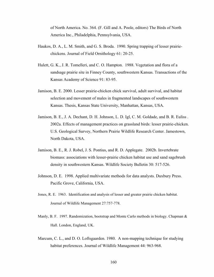
of North America. No. 364. (F. Gill and A. Poole, editors) The Birds of North

America Inc., Philadelphia, Pennsylvania, USA.









Jamison, B. E., J. A. Dechant, D. H. Johnson, L. D. Igl, C. M. Goldade, and B. R. Euliss .

2002a. Effects of management practices on grassland birds: lesser prairie-chicken.

U.S. Geological Survey, Northern Prairie Wildlife Research Center. Jamestown,

North Dakota, USA.

Jamison, B. E., R. J. Robel, J. S. Pontius, and R. D. Applegate. 2002b. Invertebrate

biomass: associations with lesser-prairie chicken habitat use and sand sagebrush

density in southwestern Kansas. Wildlife Society Bulletin 30: 517-526.

Johnson, D. E. 1998. Applied multivariate methods for data analysts. Duxbury Press.

Pacific Grove, California, USA.

Jones, R. E. 1963. Identification and analysis of lesser and greater prairie chicken habitat.

Journal of Wildlife Management 27:757-778.

Manly, B. F. 1997. Randomization, bootstrap and Monte Carlo methods in biology. Chapman &

Hall. London, England, UK.

Marcum, C. L., and D. O. Loftsgaarden. 1980. A non-mapping technique for studying

habitat preferences. Journal of Wildlife Management 44: 963-968.

160

Nams, V. 2000. Locate II: user’s guide. Pacer Computer Software, Truro, Nova Scotia,

Canada.

Oyler-McCance, S. J. 1999. Genetic and habitat factors underlying conservation

strategies for Gunnison sage-grouse. Dissertation, Colorado State University, Fort

Collins, Colorado, USA.







Taylor, M. A., and F. S. Guthery. 1980. Fall-winter movements, ranges, and habitat use

of lesser prairie-chickens. Journal of Wildlife Management 44: 521-524.


threatened wildlife and plants; review of species that are candidates that are

proposed for listing as endangered or threatened: the lesser prairie-chicken.

Federal Register 67: 40667.


Game Magazine 1-4.




Worton, B. J. 1989. Kernel methods for estimating the utilization distribution in home-

range studies. Ecology 70:164-168.

161

Tabl

e 1.

Par

amet

er e

stim

ates

of h

abita

t and

land

scap

e fe

atur

es fo

r les

ser p

rairi

e-ch

icke

n us

e, n

on-u

se a

nd a

bsen

t site

s. M

eans

and

stan

dard

err

ors a

re p

rese

nted

for m

easu

red

varia

bles

alo

ng w

ith th

e st

anda

rdiz

ed c

anon

ical

scor

es (C

AN

-1 a

nd C

AN

-2) f

or e

ach

varia

ble.

Col

umns

with

diff

eren

t let

ters

indi

cate

a si

gnfic

ant d

iffer

ence

(P <

0.0

5).

Are

a ty

pe

Stan

dard

ized

can

onic

al sc

ores

Var

iabl

e

Use

Non

-use

Abs

ent

C

AN

-1C

AN

-2Sh

rub

cove

r (%

) 15

.3 ±

3.1

A

13.6

± 3

.1A

35

.0 ±

3.1

B

0.42

8 -0

.559

Forb

cov

er (%

) 9.

7 ±

1.4A

7.

7 ±

1.4A

8.

9 ±

1.5A

0.44

10.

015

Gra

ss c

over

(%)

13.4

± 1

.7A

14

.3 ±

1.6

A

14.1

± 1

.7A

-0

.360

-0.5

21

Litte

r cov

er (%

) 29

.9 ±

2.4

A

38.6

± 2

.4B

16

.4 ±

2.5

C

0.24

80.

028

Shru

b de

nsity

(m2 )

2.5 ±

0.2A

2.

0 ±

0.2A

4.

4 ±

0.2B

0.

870

0.29

0

Shru

b di

am (c

m)

71.0

± 3

.2A

67

.7 ±

3.1

A

80.1

± 3

.3B

0.

217

-0.2

13

Dis

tanc

es (m

)

W

ells

43

5.0 ±

31.2

A

446.

0 ±

30.8

A

323.

2 ±

31.6

B

-0.3

820.

104

Roa

ds

193.

2 ±

18.7

A

178.

8 ±

18.6

A

184.

4± 1

9.0A

-0

.071

0.11

4

Stru

ctur

e 1,

397 ±

106A

1,

061 ±

105B

75

9 ±

108C

-0

.332

-0.0

40

Pow

erlin

es

1,10

6 ±

81A

66

6 ±

80B

70

5 ±

82B

-0

.060

1.02

4

162

Table 2. Canonical scores and sagebrush density plants ha-1 ( x ± SE) of

lesser prairie-chicken use area type. Differences in usage area type are defined in the text.

Area type

Variate/ sagebrush Use Non-use Absent

CAN-1 – 0.561 ± 0.158 – 0.926 ± 0.154 1.694 ± 0.158

CAN-2 0.591 ± 0.158 – 0.472 ± 0.154 – 0.069 ± 0.158

Sagebrush density ha-1 3,144 ± 249 2,553 ± 201

7,205 ± 573

163

Table 3. Count data of landscape features for contingency table and Poisson rate

regression modeling of lesser prairie-chicken monthly-ranges.

Year Apr May Jun Jul Aug Sep

2000 No. ranges 30 8 21 23 17 17

Avg. ha 553 667 273 170 148 180

Points in ranges 111,493 72,929 5,258 33,076 35,084 3,561

Roads (points) 2,597 1,575 1,127 617 829 752

Powerlines (points) 150 58 37 26 38 27

No. wells 52 44 21 10 13 8

2001 No. ranges 15 9 18 24 25 23

Avg. ha 805 1045 396 182 119 151

Points in ranges 97,064 107,238 78,575 42,787 41,272 34,033

Roads (points) 2233 2522 2025 1024 951 763

Powerlines (points) 144 213 398 54 38 60

No. wells 44 58 39 17 19 13

2002 No. ranges 11 8 16 16 ND

ND

Avg. ha 584 231 306 135 ND ND

Points in ranges 61,526 27,107 64,288 30,491 ND ND

Roads (points) 1,729 600 1,420 672 ND ND

Powerlines (points) 540 241 518 186 ND ND

No. wells 24 12 34 10 ND ND

164

Fig 1. Mean canonical variates (CAN-1 and CAN-2), SEs (in both x,y) and their

respective 95 % confidence circles for lesser prairie-chicken use, non-use and absent

sites. CAN-1 was best explained by high sagebrush densities and large shrubs. Distances

to structures and wells also explained CAN-1, but were negatively related. This revealed

that that absent sites were in closer proximity to these anthropogenic features than other

sites. CAN-2 was best explained by distance to powerlines. Although these sites

separated in a 2-dimensional space, use and non-use did not differ in regards to their

mean value of CAN-1, but both differed from the mean CAN-1 score of absent sites.

Alternatively, non-use and absent sites were similar with respect to CAN-2 but differed

from use sites, suggesting that distance to powerlines was important in determining

suitability of lesser prairie-chicken habitat.

165

Canonical variate-1

-1 0 1 2

Can

onic

al v

aria

te-2

-1

0

1

2

Use

Non-use

Absent

166

Fig. 2. Odds ratios (95% confidence limits) for roads occurring in lesser prairie-chicken

monthly-ranges in 2000 (A), 2001 (B), and 2002 (C). The dashed line indicates odds of

1 and confidence limits intersecting this line indicate odds not different than expected by

chance.

167

2000

Apr May Jun Jul Aug Sep

Odd

s of

road

s in

mon

thly

-rang

e

0.6

0.7

0.8

0.9

1.0

1.1

2001

Apr May Jun Jul Aug Sep0.80

0.85

0.90

0.95

1.00

1.05

1.10

1.15

2002

Apr May Jun Jul0.7

0.8

0.9

1.0

1.1

1.2

1.3

(A) (B)

(C)

168

Fig. 3. Odds ratios (95% confidence limits) for powerlines occurring in lesser prairie-

chicken monthly-ranges in 2000 (A), 2001 (B), and 2002 (C). The dashed line indicates

odds of 1 and confidence limits intersecting this line indicate odds not different than

expected by chance.

169

2000


0.05

0.10

0.15

1.00

2001


0.1

0.2

0.3

0.4

0.5

0.6

0.7

0.8

0.9

1.0

2002

Apr May Jun Jul0.4

0.5

0.6

0.7

0.8

0.9

1.0

Odd

s of

pow

erlin

es in

mon

thly

-rang

e

(A) (B)

(C)

170

Fig. 4. Differences in the mean number (95% confidence limits) of wells ha-1,000 between

monthly- and non-ranges as determined from Poisson rate regression. The dashed line

indicates a difference of 0 and confidence limits intersecting this line indicate a observed

values did not differ from those expected by chance.

171

Apr May Jun Jul Aug Sep

Diff

eren

ce in

no.

of w

ells

ha-1

,000

(95%

CL)

-1.2

-1.0

-0.8

-0.6

-0.4

-0.2

0.0

0.2

0.4

172

OVERALL STUDY SUMMARY

Introduction

The lesser prairie-chicken (Tympanuchus pallidicinctus) has sustained marked

reductions in suitable habitat over the past 100 years. The remaining habitat is widely

used for petroleum exploration and extraction, cattle grazing, powerline easements, and

the generation of electricity. It is estimated that over 90% of the range has been lost since

the turn of the 20th century and the range wide population has paralleled these losses. In

1995, the lesser prairie-chicken was petitioned to be listed as threatened under the

Endangered Species Act. Given the status of this sensitive species it is critical to

understand the dynamics of local and regional populations and possible management

scenarios that would most effectively benefit the lesser prairie-chicken.

This study is the culmination of two Federal Aid in Wildlife Restoration projects,

W-47-R and W-53-R. Field work for W-47-R began in spring 1997 and was completed

in November 1999, and W-53-R was initiated in December 1999 and concluded in March

2003. Project W-47-R was located on a 5,700-ha fragment of sand sagebrush prairie

(Area I) south of the Arkansas River (~ 4 km south of Holcomb, Finney County, Kansas).

Project W-53-R added second study site (Area II) of 5,400 ha. The center of Area II was

~20 km east of Area I. Research was conducted simultaneously on both sites from spring

2000 through spring 2003. Primary research objectives were to gather information on

specific demographic parameters and examine population viability and sentivity to

changes in the parameters.

173

A total of 755 lesser prairie-chickens were captured and banded from 1997 to

2002, and 136 male (46 yearling, 66 adult, 24 age undetermined), and 227 female (87

yearling, 117 adult, and 23 age undetermined) were fitted with radio transmitters.

Radiomarked birds were tracked daily using vehicle mounted antennae, resulting in

39,969 daily bird locations. These data were used to determine nest success, chick

survival, adult survivorship, habitat usage, and the resulting parameter estimates were

used as inputs to the demographic model.

Age-specific survival of males

Robust estimates of annual survival are useful for two reasons: understanding

management efforts and basic science. Survival is one of several demographic rates that

can effect the fluctuations in population numbers of grouse and the occurrence of age-

specific survival and reproductive rates may covary with the type of mating system in

grouse. Three hundred and seventy-six male prairie-chickens (173 yearlings, 203 adults)

were captured from 1998-2002, and 150 males (78 yearlings, 72 adults) were recaptured

at least once. Analyses of live mark-recapture data were used to estimate survival. Local

survival rates (φ) of male lesser prairie-chickens were highest for yearling (φ1 = 0.615) >

adult (φ1 = 0.485) > older adults (φ2 = 0.347). Twenty percent of recaptured yearlings

switched leks in their second year, and were 2.5 (odds ratio) times as likely than adults to

do so (8%). Each age-class was equally likely (~17.5 %) to move between leks within a

breeding season. Four and 15 % of yearlings and adults were recaptured > 3 times,

respectively. This suggests that adults had a greater propensity to attend leks and

presumably try to obtain copulations than yearlings. The overall estimates of lesser

174

prairie-chicken survival were slightly elevated when compared to that of other banding

studies of prairie grouse.

Effects of radiomarking on lesser prairie-chicken survival

Radiotelemetry has provided wildlife biologists a tool to estimate survival where

fate of each individual is likely known. While these analyses of these data can result in

highly accurate estimates, five assumptions must be met. Two of the assumptions,

random right-censoring and no-transmitter effect on survival, are often difficult to assess

in studies. Male lesser prairie-chickens in this study were not measurably impacted by

radiomarking, as their survival rates were greater than or equal to those of banded birds.

The model best supported by the data, Sc, pgroup+t, rg, Fc, indicated that survival was best

modeled as constant (Ŝc = 0.731, SE = 0.072) across radiomarked and banded birds.

Signal loss occurred throughout the monitoring period and appeared to be independent of

periods of high mortality. Eight of 16 (50%) right-censored birds were subsequently

recaptured, which was similar to the recapture rates for known-fate birds (55.8%),

suggesting that right-censored birds had similar survival rates to that of known-fate

individuals.

Survival of male and female lesser prairie-chickens

In total, 136 male (46 yearling, 66 adult, 24 age undetermined), and 227 female

(87 yearling, 117 adult, and 23 age undetermined) lesser prairie-chickens were captured

and fitted with radio transmitters. Year to year variation in summer survival was evident

and seemed to be highly related to mortality rates of incubating females on nests and

>30% of all female mortality was associated with the nesting period. Summer survival

rates (Apr-Nov) and apparent nest success from 5 years revealed the strength of this

175

relationship. Gender-specific survival was not well supported by the data, as the overall

survival rates of males and females were similar in the summer (Smale = 0.69 ; Sfemale =

0.67) and seasonal (Apr-Mar) analyses (Smale = 0.39; Sfemale = 0.43). However, the

timing of survival over 12-months suggested that seasonal patterns in male survivorship

do not match the temporal pattern seen in females.

Age-specific patterns in female survival were evident in both analyses with

yearling birds (Ssummer = 0.75; Sseasonal = 0.52), surviving at a higher rate than adults

(Ssummer = 0.69, Sseasonal = 0.37). One explanation for this difference is the cost of

reproduction, as it may result in reduced survival rates of adults, if they had higher

reproductive output, but, reproductive parameters were similar between age-classes in

this study. Management of lesser prairie-chickens should focus on habitat manipulations

that increase nest survival and decrease female losses during incubation. In fragmented

populations, predator control may achieve short-term goals of increased female survival

and nest success, but may be too costly to sustain in the long-term


One-hundred and thirty four mortalities were recorded from spring 1997 to spring

2003, and the majority of mortality was attributed to mammalian predation (54%). Males

seemed more susceptible to raptor predation (20%) than females (11%) but were not

measurably different. Seven of the eight accidents were associated with powerline

collisions. Losses to recreational hunting were small (5%) relative to the radiotelemetry

population, but even less (1.2%) when compared to banded birds that were available for

harvesting. Males apparently were more susceptible to hunting losses than females.

176

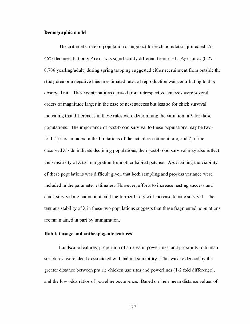
Demographic model

The arithmetic rate of population change (λ) for each population projected 25-

46% declines, but only Area I was significantly different from λ =1. Age-ratios (0.27-

0.786 yearling/adult) during spring trapping suggested either recruitment from outside the

study area or a negative bias in estimated rates of reproduction was contributing to this

observed rate. These contributions derived from retrospective analysis were several

orders of magnitude larger in the case of nest success but less so for chick survival

indicating that differences in these rates were determining the variation in λ for these

populations. The importance of post-brood survival to these populations may be two-

fold: 1) it is an index to the limitations of the actual recruitment rate, and 2) if the

observed λ’s do indicate declining populations, then post-brood survival may also reflect

the sensitivity of λ to immigration from other habitat patches. Ascertaining the viability

of these populations was difficult given that both sampling and process variance were

included in the parameter estimates. However, efforts to increase nesting success and

chick survival are paramount, and the former likely will increase female survival. The

tenuous stability of λ in these two populations suggests that these fragmented populations

are maintained in part by immigration.

Habitat usage and anthropogenic features

Landscape features, proportion of an area in powerlines, and proximity to human

structures, were clearly associated with habitat suitability. This was evidenced by the

greater distance between prairie chicken use sites and powerlines (1-2 fold difference),

and the low odds ratios of poweline occurrence. Based on their mean distance values of

177

759 and 323 m, structures and wells were significantly closer to sampling points,

respectively, on the absent site than either use or non-use sites. However, non-use sites

were 336 m closer to structures than use sites. Monte Carlo simulations indicated that

≥60% of lesser prairie-chicken centers of use were further from anthropogenic features

than would be expected at random. Combined, these data suggest that lesser prairie-

chickens used areas with less anthropogenic disturbance.

The relationship of habitat usage as it pertains to sagebrush density and cover may

be non-linear. Future impact assessments and conservation plans should consider the

construction or presence of anthropogenic features as a potential detriment to habitat

suitability for lesser prairie-chickens. Habitat inventories should carefully consider the

proximity and density of anthropogenic features when prioritizing habitat patches for

conservation action or mitigation. Further work is needed to clarify the potential non-

linear relationship between habitat suitability and sagebrush stand characteristics.

178

APPENDIX I

A RANGE-WIDE GENETIC EVALUATION OF LESSER PRAIRIE-CHICKENS

INTRODUCTION

The current distribution of the lesser prairie-chicken (Tympanuchus

pallidicinctus) is highly fragmented throughout the species’ range, and its habitat is

widely used for agriculture, housing developments, petroleum exploration and extraction,

cattle grazing, power line easements, and the generation of electricity. The cumulative

loss of habitat and declining population trends led to the “warranted but precluded”

threatened listing under the Endangered Species Act (U.S. Fish and Wildlife Service

2002).

It has been hypothesized that genetic factors may be contributing to the observed

population trends. Such was the case for remnant greater prairie-chicken (T. cupido)

populations in Illinois and Wisconsin that sustained a population bottleneck (Bouzat et al.

1998, Bellinger et al. 2003). The demographic and genetic consequences were reduced

fertility and heterozygosity, respectively (Bouzat et al. 1998). Could similar processes be

at work with the lesser prairie-chicken when populations have been substantially

reduced? Van Den Bussche et al. (2003) found reasonable levels of heterozygosity (both

in mitochondrial DNA and in the nuclear genome) of lesser prairie-chickens in Oklahoma

and New Mexico, suggesting that genetic variation is not limiting to population growth.

This paper expands on Van Den Bussche et al. (2003) and includes 4 populations from

Kansas and 1 from southeastern Colorado. Mitochondrial DNA (mtDNA) was evaluated

for all populations but microsatellites were only assessed for 2 fragments of sand

179

sagebrush (Artemisia filifolia) prairie in Finney County (Finney-1 and Finney-2) and 1 in

Kearny County, Kansas at the time of this report.

METHODS

Study areas

Populations were from 6 counties in Kansas (Fig. 1), 3 north (Gove, Trego, and

Ness) and 3 south (Comanche, Finney, Kearny) of the Arkansas River. Populations in

Baca and Prowers counties Colorado were also sampled. Because of small sample sizes

and genetic similarities Baca and Prowers, and Gove, Trego, and Ness counties were

pooled into 2 populations and referred to as Colorado and Gove, respectively. Range-

wide comparisons of mtDNA were made to populations previously described in Van den

Bussche et al. (2003). Comparisons were made on the county level instead of a lek-by-

lek level, and included Harper (pooling Harper and Ellis) and Beaver, Oklahoma, and

Roosevelt, New Mexico (hereafter New Mexico). The methods below refer only to the

sampling conducted between 2000 and 2002, although protocols for sequencing mtDNA

were in place to ensure consistency with Van den Bussche et al. (2003).

Tissue collection

Blood samples were obtained from lesser prairie-chickens (n = 127) captured in

funnel traps during the spring and fall (2000-02) (Haukos et al. 1991). Blood samples

were obtained by clipping a toenail of each lesser prairie-chicken and placing 2–3 drops

of blood into a microfuge tube previously coated with EDTA. All blood samples were

frozen at –20 °C.

DNA extraction and mtDNA sequencing

DNA was extracted from muscle tissue using either a phenol-chloroform method

180

(Kahn et al. 1999) or the Wizard Genomic DNA Purification System (Promega)

following the manufacturer’s instructions, except that 478 base pairs were examined.

Sequences were aligned using Gene Tool Lite 1.0 (Double Twist Inc.), and each unique

sequence was assigned a different haplotype designation.

Microsatellite genotype scoring

To evaluate finer scaled population structuring, variation in the nuclear genome

was assessed by genotyping microsatellite loci of the 3 populations from which there

were field data to compare movement rates (2 from Finney and 1 from Kearny County).

Six primers for microsatellite loci (ADL23, ADL42, ADL44, ADL146, ADL162,

ADL230) originally isolated from domestic chicken (Gallus gallus) and shown to be

variable in greater prairie-chicken (Tympanuchus cupido; Bouzat et al. 1998), and 4 loci

(SGCA5, SGCA9, SGCA11) developed for sage-grouse (Centrocercus spp.; Taylor et al.

2003), and 1(LLST1) developed for red grouse (Lagopus lagopus scoticus; Piertney et al.

1999) were used to evaluate genetic variability within the nuclear genome. The

extraction and microsatellite scoring follows Tayor et al. (2003). A standard 25 µl PCR

(Quinn 1992) was performed for each locus (MJ Research PTC-200) using a dye-labeled

forward primer and an unlabeled reverse primer. The temperatures and times of the

profiles were as follows: denaturation, 95°C for 1 minute; annealing, 60°C for 1 minute;

extension, 72°C for 1 minute. Each PCR had 35 amplification cycles. A touch-down

thermal profile was performed with all loci as follows: 1) pre-heat, 94°C for 1 minute; 2)

denaturation, 92°C for 5 seconds; annealing, 66°C to 56°C (-0.5°C per cycle) for 30

seconds; 3) denaturation, 92°C for 5 seconds; annealing, 55°C for 30 seconds (+1 second

per cycle); 4) final extension, 72°C for 10 minutes. Each denaturation and annealing

181

combination (2 and 3) cycled 20 times before the next step so that a total of 40 cycles

were performed. Samples were run on the CEQ2000 XL DNA Analysis System

(Beckman-Coulter). The SGCA11 samples were run with the S600 size standard using

the Frag 4 default method. All other loci were run with the S400 standard and the Frag 3

default method.

Data Analyses

Mitochondrial DNA.–Estimates of haplotype (h) and nucleotide (π) diversity

within populations were calculated in ARLEQUIN 2.0 (Schneider et al. 2000). Analysis

of molecular variance (AMOVA) was used to quantify haplotype diversity at 3 different

levels of a hierarchy. State and geographic regions (i.e., sand sagebrush prairie of Kansas

and Colorado: Finney, Kearny, and Prowers; mixed-grass prairie of Kansas: Gove;

mixed-shrub of Kansas: Comanche; mixed shrub of Oklahoma: Beaver and Harper; and

sand shinnery oak [Quercus havardii] of New Mexico) was 1 level, the variation among

populations within a region was the second level, and variation among individuals within

populations as the third level. Population subdivision was examined in ARLEQUIN 2.0

(Schneider et al. 2000) using significance tests of pairwise population FST values. An F-

test was calculated to determine whether the distribution of haplotypes among

populations differed. The molecular distances between haplotypes was calculated using

Nei’s unbiased minimum distance (Nei 1978), and neighbor-joining trees were

constructed showing the relationships among the 8 populations.

Microsatellites.–Allele frequencies, mean number of alleles per locus, deviations

from Hardy-Weinberg expectation, and population differentiation were quantified in

ARLEQUIN 2.0 (Schneider et al. 2000). Each locus at each population was tested for

182

deviations from Hardy-Weinberg expectations and P < 0.05 was the criterion for

statistical significance. AMOVA and pairwise RST statistics were used to examine

variation among populations and population subdivision, respectively.

RESULTS

Two-hundred and ninety-three lesser prairie-chickens were captured in Kansas

and Colorado between 2000 and 2002: Finney-1 = 90, Finney-2 = 93, Kearny = 28,

Comanche = 17, Gove = 45, and Colorado = 20. Due to logistics DNA was extracted

from a sub-sample of birds from Finney-1 and –2, resulting in 127 samples for Kansas

and Colorado.

Mitochrondrial DNA

There were 45 different haplotypes across all individuals from both studies (n =

278), 31 of which had been previously described in Van den Bussche et al. (2003).

Haplotypes A, B, C, and J were the most common haplotypes and each occurred in 5 to 8

of the populations (Fig. 2). Twenty-two unique haplotypes were found; Gove (7), Harper

(7), New Mexico (3), Kearny (2), Beaver (2), and Comanche (1).

Within-population haplotype diversity (h), which represents the number and

frequency of haplotypes was generally high for all populations, but New Mexico had the

lowest (83%). Moderate levels of nucleotide diversity (π) were present in most

populations, but again New Mexico had the lowest (0.7%). Genetic diversity attributable

to variation within populations, among populations within regions, and between regions

was partitioned as 94.2%, 1.4%, an, 4.4%, respectively. Pairwise FST tests indicated

substantial population differentiation (Table 2). New Mexico was statistically different

183

from all other populations, Finney, Beaver, and Gove were statistically different from

most other populations.

Neighbor-joining tree analysis (Fig. 3) reflected the differences observed in the

pairwise comparisons, and found substantial population structure among the 8

populations that is consistent with 4 geographic subdivisions of the populations: Kansas

(Finney, Kearny [south of Arkansas River]) and Colorado; Kansas (Gove [north of

Arkansas River]); Oklahoma (Beaver, Harper) and Kansas (Comanche[south of

Arkansas River ]); and New Mexico.

Microsatellites

All individuals (n = 94) from Finney-1, Finney-2, and Kearny were examined for

8 microsatellite loci, because of difficulties in scoring LLST1, it was removed from all

analyses. SGCA11 had a significant departure from Hardy-Weinberg equilibrium for

Finney-1 (P = 0.011) and Finney-2 (P = 0.014) and was not considered in further

analyses. Additionally SGCA9 had 21 alleles which was > 2-fold of any other loci, thus

it was not included in further analyses. Several alleles were found at each of the

remaining 5 loci and all were polymorphic (Table 3). The proportions of genetic

diversity were partitioned as 77.4% within and 22.6% between populations. An exact test

of population differentiation based initially on pairwise RST statistics found significant

differentiation between Finney-1 and Kearny (P = 0.011), Finney-2 and Kearny (P =

0.013), but not between Finney-1 and Finney-2 (P = 0.377).

DISCUSSION

These lesser prairie-chicken populations were found to have relatively high levels

of genetic diversity as was indicated by average heterozygosity and number of haplotypes

184

found within and among populations. However, the large number of base-pairs (478)

examined in this study contributed to the large number of haplotype designations. A

transversion analysis (that redefines haplotypes based on the rarity of a base-pair switch)

may yield additional insights to population structuring. Birds from New Mexico had the

fewest haplotypes, and were markedly different from other populations as evidenced by

pairwise FST and neighbor-joining tree analyses. This suggests that this lesser prairie-

chicken population has been isolated from the populations in the northeastern range.

Although there was lower genetic diversity in this population, no deleterious effects to

demographic rates have been documented (D. H. Wolfe, Sutton Research Center,

unpublished data).

Pairwise FST tests (P < 0.002) indicated substantial population structuring among

the 8 populations, and was consistent with geographic subdivision of populations: Kansas

(Finney, Kearny[south of Arkansas River]) and Colorado; Kansas (Gove [north of

Arkansas River]); Oklahoma (Beaver, Harper) and Kansas (Comanche[south of Arkansas

River]); and New Mexico. This genetic and geographic structure suggests that birds

north of the Arkansas River in Kansas have been separate from birds south of the River

for many years, however, time since divergence has not been calculated. The geographic

structuring of mtDNA appears to follow the general habitat types, sand sagebrush prairie

of Kansas and Colorado, mixed-grass prairie of Kansas, mixed-shrub of Kansas and

Oklahoma, and sand shinnery oak of New Mexico, which is probably an artifact of

habitat fragmentation at a larger scale, but also could reflect genotypes adapted for these

regional environmental gradients.

185

Microsatellite analyses of adult males from the Finney and Kearny populations

indicated that male genetic structuring may be more pronounced at fine scales than was

realized by the mtDNA analyses. Such localized genetic flow of males is logical given

that juvenile males generally do not disperse >2 km from their natal site (Pitman 2003).

Alternatively, the mtDNA analyses included females and indicated no differentiation

between these populations indicating that females likely are responsible for most of the

genetic diversity across these populations. This was evidenced in part by radiotelemetry

studies from Finney County that indicated a 20% emigration rate (Chapter 3) of all

radiomarked birds (only 2 were males), and these birds moved between 20 and 50 km

from the county to other sagebrush fragments.

Studies of greater prairie-chicken genetics have found reduced numbers of alleles

in contemporary populations (7) compared to those of historic populations (9.2)

(Bellinger et al. 2003). Bouzat et al. (1998) documented >5 alleles in all populations

except Illinois, which had 3.7 alleles per locus. Van den Bussche et al. (2003) reported

5.8 and 4.8 alleles per locus in Oklahoma and New Mexico lesser prairie-chicken

populations, respectively, that had > 20 samples. This was comparable to the number of

alleles found in this study 4.8–5.0. What is less clear is the relationship of these allelic

frequencies compared to historic samples.

LITERATURE CITED

Bellinger, M. R., J. A. Johnson, J. Toepfer, and P. Dunn. 2003. Loss of genetic variation

in greater prairie-chickens following a population bottleneck in Wisconsin U.S.A.

Conservation Biology 17: 717–724.

Benedict, N. G., S. J. Oyler-McCance, S. E. Taylor, C. E. Braun, and T. W. Quinn. 2003.

Evaluation of the eastern (Centrocercus urophasianus urophasianus) and western

186

(Centrocercus urophasianus phaios) subspecies of sage-grouse using

mitochondrial control-region sequence data. Conservation Genetics 4: 301-310.

Bouzat, J. L., H. H. Cheng, H. A. Lewin, J. D. Brawn, R. L. Westemeier, and K. N.

Paige. 1997. Genetic evaluation of a demographic bottleneck in greater prairie-

chicken. Conservation Biology 12: 836–843.


chickens. Journal of Field Ornithology 61: 20–25.

Kahn N. W., C. E. Braun, J. R. Young, S. Wood, D. R. Mata, and T.W. Quinn. 1999.

Molecular analysis of genetic variation among large- and small-bodied sage

grouse using mitochondrial control-region sequences. Auk 116: 819–824.

Oyler–McCance, S. J., N. W. Kahn, K. P. Burnham, C. E. Braun, and T. W. Quinn. 1999.

A population comparison of large– and small–bodied sage grouse in Colorado

using microsatellite and mitochondrial DNA markers. Molecular Ecology 8:

1457–1465.




Quinn, T. W. 1992. The genetic legacy of Mother Goose–phylogenetic patterns of lesser

snow goose Chen carulescens carulescens maternal lineages. Molecular Ecology

1: 105–117.

Taylor, S. E., S. J. Oyler-McCance, and T. W. Quinn. 2003. Isolation and

characterization of microsatellite loci in Greater Sage-Grouse (Centrocercus

urophasianus). Molecular Ecology 12: In press

Schneider, S., D. Roessli, and L. Excoffier. 2000. Arlequin version 2.0: a software for

population genetics data analysis . Biometry Laboratory, University of Geneva.

Geneva, Switzerland.


187

threatened wildlife and plants; review of species that are candidates or proposed

for listing as endangered or threatened: the lesser prairie-chicken. Federal

Register 67: 40667.

Van den Bussche, R. A., S. R. Hoofer, D. A. Wiedenfeld, D. H. Wolfe, and S. K.

Sherrod. 2003. Genetic variation within and among fragmented populations of

lesser prairie-chickens (Tympanuchus pallidicinctus). Molecular Ecology 12:

675–683.

188

Table 1. Descriptive statistics based on DNA sequence data of a portion of the mtDNA

D-loop for 8 lesser prairie-chicken populations.

mtDNA statisticsa

Population location n A h (SE) π (SE)

Finney, KS 35 14 0.919 (0.021) 0.014 (0.008)

Kearny, KS 24 12 0.909 (0.038) 0.080 (0.040)

Gove, KS 39 20 0.947 (0.020) 0.012 (0.007)

Comanche, KS 14 9 0.912 (0.059) 0.069 (0.036)

Beaver, OK 27 12 0.912 (0.028) 0.012 (0.007)

Harper, OK 61 23 0.944 (0.012) 0.014 (0.007)

Prowers, CO 15 10 0.952 (0.034) 0.012 (0.007)

Roosevelt, NM 63 9 0.828 (0.027) 0.007 (0.004)

a n = sample size, A = number of haplotypes, h = haplotype diversity, and π = nucleotide

diversity.

189

Table 2. Significance (P < 0.0017) of pairwise FST tests for mtDNA sequencing data from

8 populations of lesser prairie-chickens in 4 states. Pairs of populations significantly

different are shown by + and those not significantly different are shown by –.

Population

Population

location

Finney Kearny Gove Coman

-che

Beaver Harper Colo.

Kearny, KS –

Gove, KS + +

Comanche, KS + – –

Beaver, OK + + + –

Harper, OK + – + – –

Prowers, CO – – – – + –

Roosevelt, NM + + + + + + +

190

Table 3. Number of alleles and average expected and observed heterozygosity at 5

microsatellite loci for 3 populations of lesser prairie-chickens in southwestern Kansas.

Microsatellite statisticsa

Population location n A HO (SD) HE (SD)

Finney-1, KS 32 4.8 0.453 (0.121) 0.505 (0.132)

Finney-2, KS 35 5.0 0.530 (0.116) 0.550 (0.116)

Kearny, KS 27 4.8 0.451 (0.079) 0.536 (0.094)

a n = sample size, A = average number of alleles, HO = mean observed heterozygosity,

and HE = mean expected heterozygosity under Hardy-Weinberg equilibrium.

191

Fig. 1. Sampling locations (black dots) and counties (gray polygons) of lesser prairie-

chickens for genetic evaluations. Rivers indicated by black irregular lines. Oklahoma

and New Mexico sites are from Van den Bussche et al. (2003).

192

Fig. 2. Frequency of 45 haplotypes (pie charts) by geographic region and sampling sites.

Shaded areas depicts current range of lesser prairie-chickens.

194

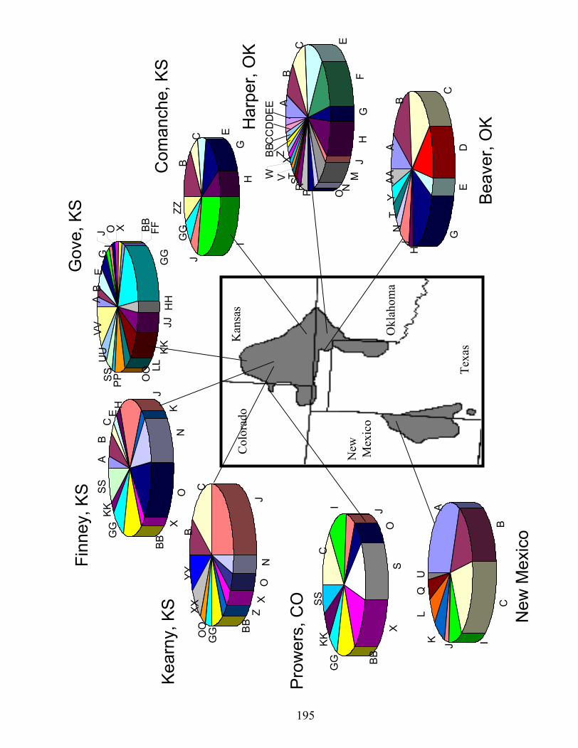
Gov

e, K

S

Kear

ny, K

S

Har

per,

OK

CI J

OS

X

BBGG

KKSS

AB

EG

IJ O X BB FF

GG

HH

JJKK

LLO

O

PPSSU

UVV

AB

CE

H

JK

NO

X BB

GG

KKSS

BC

JN

OX

Z BB

GGOO

XXYY

H

BC E

GI

JG

GZZ

AB

CD

EG

HJ

NT

YAA

A

BC

IJKL

QU

Com

anch

e, K

S

AB

C EF

GH

JM

NOPRSTVWXZBB

CC

DD

EE

Texas

New Mexico

Colorado

Kansas

Oklahoma

Finn

ey, K

S

Prow

ers,

CO

195

Beav

er, O

K

New

Mex

ico

Fig. 3. Neighbor-joining tree based on Nei’s unbiased minimum distance, habitat

specific populations denoted by ellipses and labeled in rectangular boxes. Note the

relationship to the geographic structuring of populations reflected in Fig. 2.

196

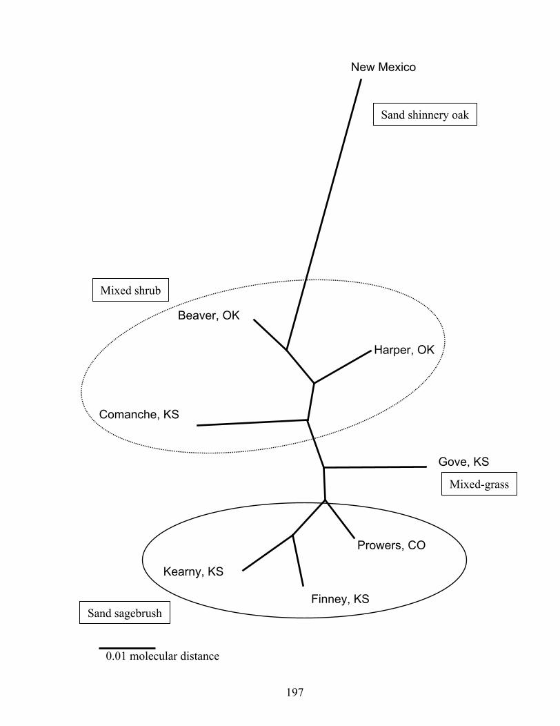
Gove, KS

Prowers, CO

Finney, KS

Kearny, KS

Comanche, KS

Beaver, OK

New Mexico

Harper, OK

0.01 molecular distance

Sand sagebrush

Mixed shrub

Sand shinnery oak

Mixed-grass

197

APPENDIX II

TABLES OF LESSER PRAIRIE-CHICKEN MORPHOMETRICS

Appendix 2A. Morphometrics ( x ± SD) of yearling and adult male and female lesser

prairie-chickens Finney County, Kansas 1998–2002.

Age

Measurementa n Yearlingb n Adult Pooled

Wing-chord(mm)

Female 3 201.3 ± 4.2 10 202.9 ± 5.4 202.5 ± 4.9

Male 10 205.4 ± 3.9 19 209.6 ± 3.6 208.2 ± 4.1

Tarsus (mm)

Female 3 49.0 ± 1.4 10 47.4 ± 3.7 47.8 ± 3.4

Male 10 47.7 ± 2.2 20 49.4 ± 2.2 48.8 ± 2.3

Foot (mm)

Female 3 52.7 ± 2.5 10 51.8 ± 1.6 52.0 ± 1.9

Male 10 54.1 ± 1.9 15 54.3 ± 2.7 54.2 ± 2.4

Mass (g)b

Female 95 709.8 ± 45.3 108 748.9 ± 46.8 730.6 ± 50.3

Male 210 790.1 ± 41.6 294 806.7 ± 40.5 800.2 ± 41.0

Male (Kearny) 3 785.0 ± 27.8 25 796.7 ± 39.0 795.4 ± 29.8 a The body mass of captured birds was determined to the nearest 5 g on with a Pesola

spring scale. Calipers were used to measure tarsometatarsus (tarsus) length and an

aluminum wing-chord ruler was used to measure foot length and wing length to the

nearest 1 mm. Greatest length of the tarsus was measured from the posterior proximal to

the posterior distal. Foot length was measured from back of bent heel to end of middle

toe excluding the toenail. Wing length was measured from distal end of the carpal joint

to tip of the longest primary, wing pressed flat against ruler.

b Birds captured in March and April, yearlings ≤ 10 months and adults ≥ 22 months. c Only body mass was measured on males from Kearny County.

198

199

Appendix 2B. Morphometrics ( x ± SD) of male lesser prairie-chickens captured in

Comanche County, Kansas and Prowers County, Colorado 2002.

Age

Measurementa n Yearling n Adult Pooled

Wing-chord(mm)

Comanche 3 209.4 ± 3.6 9 208.8 ± 2.6 208.7 ± 3.0

Prowers 5 208.0 ± 1.4 9 208.9 ± 4.7 208.6 ± 4.1

Tarsus (mm)

Comanche 3 54.2 ± 1.2 9 53.3 ± 1.7 53.5 ± 1.6

Prowers 5 54.3 ± 1.3 9 53.6 ± 1.3 53.8 ± 1.3

Foot (mm)

Comanche 3 48.4 ± 0.6 9 48.3 ± 1.3 48.3 ± 1.0

Prowers 5 49.0 ± 1.0 9 47.5 ± 2.3 47.9 ± 2.1

Mass (g)b

Comanche 3 729.0 ± 57.3 9 751.7 ± 39.2 740.0 ± 48.0

Prowers 5 736.7 ± 12.5 9 764.4 ± 36.8 757.5 ± 34.6 a The body mass of captured birds was determined to the nearest 5 g on with a Pesola

spring scale. Calipers were used to measure tarsometatarsus (tarsus) length and an

aluminum wing-chord ruler was used to measure foot length and wing length to the

nearest 1 mm. Greatest length of the tarsus was measured from the posterior proximal to

the posterior distal. Foot length was measured from back of bent heel to end of middle

toe excluding the toenail. Wing length was measured from distal end of the carpal joint

to tip of the longest primary, wing pressed flat against ruler.

b Birds captured in March and April, yearlings ≤ 10 months and adults ≥ 22 months. c Note capture periods for these birds were later in the breeding season than Finney

County birds, 24 Apr in Comanche and 30 Apr to 1 May for Prowers. This may explain

the lower observed masses as compared to Finney County males (800.2 ± 41.0 g).

a demographic analysis of lesser prairie ...table 6. estimates for age-specific survival and...

Documents