a deep-learning-based geological parameterization for ... · 2 convolutional neural network-based...
TRANSCRIPT

Math Geosci (2019) 51:725–766https://doi.org/10.1007/s11004-019-09794-9
A Deep-Learning-Based Geological Parameterizationfor History Matching Complex Models
Yimin Liu1 · Wenyue Sun1 · Louis J. Durlofsky1
Received: 7 July 2018 / Accepted: 9 March 2019 / Published online: 26 March 2019© International Association for Mathematical Geosciences 2019
Abstract A new low-dimensional parameterization based on principal componentanalysis (PCA) and convolutional neural networks (CNN) is developed to representcomplex geological models. The CNN–PCA method is inspired by recent devel-opments in computer vision using deep learning. CNN–PCA can be viewed as ageneralization of an existing optimization-based PCA (O-PCA) method. Both CNN–PCA and O-PCA entail post-processing a PCA model to better honor complexgeological features. In CNN–PCA, rather than use a histogram-based regularizationas in O-PCA, a new regularization involving a set of metrics for multipoint statis-tics is introduced. The metrics are based on summary statistics of the nonlinear filterresponses of geological models to a pre-trained deep CNN. In addition, in the CNN–PCA formulation presented here, a convolutional neural network is trained as anexplicit transform function that can post-process PCA models quickly. CNN–PCAis shown to provide both unconditional and conditional realizations that honor thegeological features present in reference SGeMS geostatistical realizations for a binarychannelized system. Flow statistics obtained through simulation of random CNN–PCA models closely match results for random SGeMS models for a demanding caseinwhichO-PCAmodels lead to significant discrepancies. Results for historymatchingare also presented. In this assessment CNN–PCA is applied with derivative-free opti-mization, and a subspace randomized maximum likelihood method is used to provide
B Yimin [email protected]
Wenyue [email protected]
Louis J. [email protected]
1 Department of Energy Resources Engineering, Stanford University, Stanford, CA 94305-2220,USA
123
726 Math Geosci (2019) 51:725–766
multiple posterior models. Data assimilation and significant uncertainty reduction areachieved for existing wells, and physically reasonable predictions are also obtainedfor new wells. Finally, the CNN–PCA method is extended to a more complex nonsta-tionary bimodal deltaic fan system, and is shown to provide high-quality realizationsfor this challenging example.
Keywords Geological parameterization · History matching · Deep learning ·Principal component analysis
1 Introduction
Historymatching in the context of oil andgas reservoir engineering involves calibratinguncertain model parameters such that flow simulation results match observed data towithin some tolerance. The uncertain variables most commonly considered are poros-ity and permeability in every grid block of the model. History matching algorithms areoften most effective when combined with procedures for parameterizing these geolog-ical variables. Such parameterizations, based on, e.g., principal component analysis(PCA), serve two key purposes. Namely, they reduce the number of variables thatmust be determined through data assimilation, and they preserve, to varying degrees,the spatial correlation structure that exists in prior geological models.
In this work, a new and efficient low-dimensional parameterization technique forcomplex geological models, which incorporates a recently developed deep-learning-based algorithm known as fast neural style transfer (Johnson et al. 2016), is introduced.This new technique is referred to asCNN–PCA, since it combines convolutional neuralnetwork (CNN) approaches from the deep-learning domain and PCA. The CNN–PCArepresentation can be viewed as an extension of an existing parameterization proce-dure, optimization-based PCA (O-PCA) (Vo and Durlofsky 2014, 2015). CNN–PCAdisplays advantages over O-PCA for complex systems, especially when conditioningdata are scarce.
Previous work on low-dimensional model parameterization has involved the directuse of PCA representations (Oliver 1996; Reynolds et al. 1996; Sarma et al. 2006),discrete wavelet transform (DWT) (Lu and Horne 2000), discrete cosine transform(DCT) (Jafarpour et al. 2010), level-set methods (Chang et al. 2010; Ping and Zhang2013),K-SVD(Tavakoli andReynolds 2010), and tensor decomposition (Insuasty et al.2017) procedures. These methods address the parameterization problem in differentways, and each has advantages and limitations. For example, the DWT and DCT pro-cedures transformmodel parameters based onwavelet or cosine functions, though theydo not incorporate the prior covariance matrix of model parameters when constructingthe basis. Therefore, conditioning DCT and DWT parameterizations to prior geolog-ical information is not straightforward. PCA is based on the eigen-decomposition ofthe covariance matrix of prior models. As such, it honors only the two-point spa-tial statistics of the prior models, and thus is not directly applicable to non-Gaussiansystems.
Several methods have been proposed to extend PCA for non-Gaussian systems.Pluri-PCA, developed by Chen et al. (2016), combines PCA and truncated-pluri-
123
Math Geosci (2019) 51:725–766 727
Gaussian (Astrakova and Oliver 2015) representations to provide a low-dimensionalmodel for multi-facies systems. This procedure entails truncation of the underlyingPCA models and is thus non-differentiable. Hakim-Elahi and Jafarpour (2017) intro-duced a distance transformation to map a discrete facies model into a continuousdistance model that could be parameterized with PCA. However, this technique, likethe pluri-PCAprocedure, is currently limited to discrete systems. Kernel PCA (KPCA)generalizes PCA through a kernel formulation that acts to preserve some multipointspatial statistics (Sarma et al. 2008). The optimization-based PCA (O-PCA) procedureessentially extends PCAwith a post-processing step based on the single-point statistics(histogram) of the prior models (Vo and Durlofsky 2014, 2015). Regularized KPCA(R-KPCA) (Vo and Durlofsky 2016) can be viewed as a combination of KPCA andO-PCA. Emerick (2016) investigated the performance of PCA, KPCA, and O-PCAin the history matching of channelized reservoirs using an ensemble algorithm. Inthat study, O-PCA performed the best in terms of data assimilation and maintainingkey geological features. In addition, although KPCA and R-KPCA have some theo-retical advantages over O-PCA, it is not clear whether these more complex methodsoutperform O-PCA in problems of practical interest.
However, as illustrated later in this work, O-PCA does display limitations whenapplied to complex geomodels with little or no conditioning data. This is because O-PCA entails a post-processing of the underlying PCA model using what is essentiallya point-wise histogram transformation. The ability of O-PCA to provide models con-sistent with the training image depends on the quality of the underlying PCA model,which in turn depends on the complexity of the training image and the amount of harddata available. The point-wise post-processing step does not substantially improvethe ability of O-PCA to capture multipoint statistics. The CNN–PCA formulationintroduced here employs features for capturing multipoint spatial correlations, whichprovides enhancement relative to O-PCA for non-Gaussian systems.
Recent successes in the application of deep learning for image processing haveinspired the development of geological parameterization techniques based on algo-rithms that use deep neural networks. Among the many deep-learning procedures,the so-called deep generative models, which are used for constructing new imagesconsistent with a set of training images, are of particular interest. Deep generativemethods have been used for pore-scale model generation by Mosser et al. (2017,2018) and Wang et al. (2018). Two families of deep generative models were recentlyapplied for reservoir-scale geological parameterization: generative adversarial net-work (GAN) models (Laloy et al. 2018; Chan and Elsheikh 2017, 2018; Dupont et al.2018; Mosser et al. 2018) and autoencoder/variational autoencoder (AE/VAE) models(Laloy et al. 2017; Canchumuni et al. 2017, 2018). These procedures take realizationsof a low-dimensional random variable (called the latent variable) as input. Output cor-responds to new geological realizations. The quality of these realizations was shownto be superior to those from existing algorithms such as PCA, O-PCA, and DCT.
In this study, an alternative deep-learning-based geological parameterizationmethod, inspired by the ‘fast neural style transfer’ algorithm of Johnson et al. (2016),is developed and applied. The new method, referred to as CNN–PCA, post-processesPCA realizations to obtain models that are consistent with original realizations or areference training image. CNN–PCA can be viewed as a generalized O-PCA proce-
123

728 Math Geosci (2019) 51:725–766
dure that includes features for capturing multipoint spatial correlations. The metricsthat enter the formulation are based on statistical quantities extracted from deep convo-lutional neural networks. The (somewhat) computationally demanding optimizationcomponent of the method is performed in an offline training process of a CNN calledthe model transform net, so the online generation of models (as required in historymatching) is very fast. Extensions to handle bimodal models (as opposed to strictlybinary models) are also presented. The PCAmodels underlying the CNN–PCA proce-dure preserve the target spatial structure up to two-point correlations, so transformingthem to the final post-processed models is simpler than transforming from the latentvariable, as required in the aforementioned deep generative methods. Therefore, thetraining of the model transform net is expected to be faster than training GAN andVAE models.
This paper proceeds as follows. In Sect. 2, the CNN–PCA procedure is presented asa generalization of O-PCA, in which convolutional neural networks are applied. Next,in Sect. 3, both unconditional and conditional realizations generated using CNN–PCAare presented for a binary channelized system. Connectivity statistics are introduced inSect. 4, and these are used both to evaluate the quality of CNN–PCA realizations andfor parameter selection. In Sect. 5, the accuracy of flow statistics obtained from CNN–PCA realizations is assessed by comparison with reference geostatistical (SGeMS)realizations as well as with O-PCA models. History matching is then performed inSect. 6 to assess the ability of posterior CNN–PCAmodels to provide production fore-casts for both existing wells and new wells. Next, in Sect. 7, CNN–PCA is extended tomodel a nonstationary bimodal deltaic fan system. Concluding remarks are presentedin Sect. 8. The detailed architecture for the convolutional neural networks used inCNN–PCA is provided in the Appendix.
2 Convolutional Neural Network-Based Principal Component Analysis(CNN–PCA)
In this section the new geological parameterization, CNN–PCA, is developed. Themethod is presented as a generalized O-PCA procedure coupled with new treatmentsbased on deep convolutional neural networks.
2.1 Optimization-Based Principal Component Analysis (O-PCA)
The uncertain rock properties that characterize a reservoir model, such as permeabilityand porosity, are often represented as randomfields. In this paper, the geologicalmodelis denoted bym ∈ R
Nc×1, where Nc is the number of grid blocks (computational cells).The spatial correlation structure to be captured in m is defined by the geologicalfeatures in the reservoir.
The basic idea of PCA, also referred to as the Karhunen-Loève expansion, is torepresent the random field m using a set of variables ξ in a lower-dimensional sub-space spanned by orthogonal basis components. PCA is highly efficient for dimensionreduction and, as discussed below, enables the generation of new realizations ofm bysampling ξ from a standard normal distribution. Here, a brief description of the PCA
123

Math Geosci (2019) 51:725–766 729
procedure is provided. Refer to Sarma et al. (2008) and Vo and Durlofsky (2014) forfurther details.
The first step in PCA is to generate a set of Nr realizations of m using a geosta-tistical toolbox such as SGeMS (Remy et al. 2009). Note that throughout this paper,realizations generated using geostatistical simulation algorithms within SGeMS willbe referred to as ‘SGeMS realizations’ or ‘SGeMS models.’ Next the SGeMS realiza-tions are assembled into a centered data matrix
Y = 1√Nr − 1
[m1 − m̄ m2 − m̄ . . . mNr − m̄], (1)
where Y ∈ RNc×Nr , mi ∈ R
Nc×1 denotes realization i , and m̄ ∈ RNc×1 is the mean
of all Nr realizations. A singular-value decomposition is then performed on Y , whichgives Y = UΣV T , where U ∈ R
Nc×Nr is the left singular matrix whose columns arethe eigenvectors of YY T , Σ ∈ R
Nr×Nr is a diagonal matrix whose elements are thesquare root of the corresponding eigenvalues, and V ∈ R
Nr×Nr is the right singularmatrix.
Given U and Σ , new PCA realizations (mpca) can be generated by
mpca = UlΣlξ + m̄, (2)
where Ul ∈ RNc×l contains the l columns in U that are associated with the largest
eigenvalues, Σl ∈ Rl×l is a diagonal matrix containing the square roots of the
corresponding eigenvalues in Ul , and ξ ∈ Rl×1 is a vector with elements drawn
independently from the standard normal distribution. In practice, the variability of therandom fieldm can often be captured using relatively few PCA components (columnsin U ), which leads to l � Nc. The choice of l can be determined by applying an‘energy’ criterion (Sarma et al. 2008) or through visual inspection.
PCA performs well for Gaussian random fields, whose spatial correlation structurecan be fully characterized by two-point statistics (i.e., by the covariance matrix).However, for non-Gaussianmodelswith spatial correlation characterizedbymultipointstatistics, PCA realizations constructed using Eq. 2 do not fully honor the geologicalfeatures. O-PCA was developed by Vo and Durlofsky (2014) to provide improvedperformance for non-Gaussian models. The O-PCA formulation for binary systemswill now be described. In such systems, the value of m is either 0 or 1, where, e.g.,0 represents mud (shale) facies and 1 represents sand (channel) facies. The detailedformulation for O-PCA for bimodal systems and three-facies systems is presented inVo and Durlofsky (2015).
For binary systems, the O-PCA model is constructed by solving the followingminimization problem
mopca(ξ) = argminx
{||UlΣlξ + m̄ − x||22 + γ xT (1 − x)}, xi ∈ [0, 1]. (3)
Here, x ∈ RNc×1, xi represents the value in grid block i , and 1 ∈ R
Nc×1 is a vectorwith all components equal to 1. Equation 3 defines a minimization problem for finding
123

730 Math Geosci (2019) 51:725–766
Fig. 1 Training image for thebinary facies model of a 2Dchannelized system
50 100 150 200 250
50
100
150
200
250
0
0.1
0.2
0.3
0.4
0.5
0.6
0.7
0.8
0.9
1
the x vector thatminimizes a loss function, consisting of two termswith aweight factorγ . The first term, ||UlΣlξ + m̄ − x||22, represents the difference between x and theunderlying PCA model (Eq. 2), which ensures that the solution resembles the PCAdescription. The second term, xT (1− x), is a regularization that is a minimum (zero)when xi is either 0 or 1. It thus acts to shift the solution towards a binary distribution.The separable (block-by-block) analytical solution of Eq. 3 is provided by Vo andDurlofsky (2014). As discussed there, O-PCA realizations can be viewed as a post-processing of the corresponding PCA realization through application of a block-wisehistogram transformation.
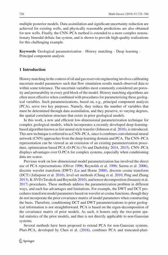
The application of PCA and O-PCA to generate new realizations of a binary faciesmodel will now be demonstrated. The conditional channelized system described inVo and Durlofsky (2014) is considered. Figure 1 displays the training image, whichcharacterizes the geological features (spatial correlation structure) and thus the mul-tipoint statistics. The training image is defined on a 250× 250 grid. In the first step, atotal of Nr = 1000 conditional SGeMS realizations are generated using the ‘snesim’geostatistical algorithm (Strebelle 2002). The model contains 60 × 60 grid blocks;therefore, Nc = 3600. Figure 2a, d shows one SGeMS realization and the correspond-ing histogram of grid-block facies type. The red and blue colors in Fig. 2a correspondto sand and mud facies, respectively. The 16 white points indicate the well locations.There are three wells in mud facies and 13 wells in sand facies. All SGeMS realiza-tions are conditioned to hard data at these well locations. The training image containsoverlapping sinuous sand channels, with general orientation of about 45◦. The SGeMSrealization (Fig. 2a) is seen to capture these features.
The PCA and O-PCA representations are constructed using a reduced dimensionl = 70 for the PCA components (Eqs. 2 and 3). In O-PCA, the weighting factor γ isset to 0.8. These values correspond to values used by Vo and Durlofsky (2014). Real-izations obtained from PCA and O-PCA, and the associated histograms, are shown inFig. 2. Both the PCA andO-PCAmodels honor all hard data. However, the PCAmodeldisplays continuous values for the facies type and does not fully capture channel con-nectivity. In addition, the corresponding histogram of grid-block facies type (Fig. 2e) isessentially Gaussian, rather than near-binary. The O-PCAmodel, by contrast, displays
123
Math Geosci (2019) 51:725–766 731
20 40 60
10
20
30
40
50
60
0
0.2
0.4
0.6
0.8
1
(a)20 40 60
10
20
30
40
50
60
-0.5
0
0.5
1
1.5
(b)20 40 60
10
20
30
40
50
60
0
0.2
0.4
0.6
0.8
1
(c)
0 0.2 0.4 0.6 0.8 1
Value
0
500
1000
1500
2000
2500
Cou
nt
(d)
-1 -0.5 0 0.5 1 1.5 2
Value
0
100
200
300
400C
ount
(e)
0 0.2 0.4 0.6 0.8 1
Value
0
500
1000
1500
2000
2500
Cou
nt
(f)
Fig. 2 Random conditional realizations obtained from SGeMS, PCA, and O-PCA for a binary channelizedsystem with hard data at 16 wells. a SGeMS realization, b PCA realization, c O-PCA realization, d SGeMSrealization histogram, e PCA realization histogram, f O-PCA realization histogram
a much sharper contrast between sand and mud facies, and the associated histogram isapproximately binary (Fig. 2f). In addition, the O-PCA model shows channel geom-etry and connectivity that is reasonably consistent with that in the SGeMS realization(Fig. 2a).
2.2 Generalized O-PCA
In the example above, the O-PCA procedure gives satisfactory results in terms ofreproducing the histogram and the geological features evident in the training image.However, as mentioned earlier, O-PCA essentially performs histogram transformationof the PCA grid-block values, which only ensures reproduction of the histogram. Aswill be shown later, formore challenging caseswhen there are fewer or no conditioning(hard) data, O-PCA realizations may not adequately capture the spatial correlationstructure inherent in the training image.
This limitation of O-PCA for non-Gaussian models is expected, since Eq. 3 doesnot account for higher-order spatial correlations. The first term in the O-PCA equation,||UlΣlξ + m̄ − x||22, penalizes O-PCA realizations that do not closely resemble theunderlying PCA realizations, and these only honor two-point correlations. The regu-larization term, xT (1−x), is a metric based only on single-point statistics (histogram).This motivates the introduction of a generalized O-PCA formulation that incorporatesmultipoint spatial statistics.
This generalized O-PCA formulation is expressed as
m(ξ) = argminx
{Lc(x,mpca(ξ)) + γs Ls(x, Mref)
}, (4)
123

732 Math Geosci (2019) 51:725–766
where mpca(ξ) denotes a PCA realization, and Mref denotes a reference model thathonors the target spatial correlation structure. The objective function consists of twoloss functions. The first loss function, Lc(x,mpca(ξ)), referred to as the content loss,quantifies the ‘closeness’ between model x and mpca(ξ) in terms of the content. Thesecond loss function, Ls(x, Mref), referred to as style loss, quantifies the degree towhich x resembles the style of Mref. ‘Style’ in this case refers to channel continuityand channel width, and the sharp contrast between sand andmud. The reference modelMref can be either a training image or a particular SGeMS realization.When the spatialrandom field is stationary, the dimension of Mref can be different from the dimensionof m. Finally, the weighting factor γs is referred to as the style weight.
The original O-PCA formulation in Eq. 3 can be viewed as one particular case ofthe generalized formulation. In this instance, the content loss is based on the Euclideandistance between x and mpca, and the style loss is based on the histogram. The styleloss in O-PCA does not explicitly contain a reference model Mref, but it is essentiallya metric for the mismatch between the histogram of x and the histogram of Mref.
In this study, a generalized O-PCA formulation with new content and style lossesis introduced in order to generate models that better honor Mref. The new loss termsare inspired by the neural style transfer algorithm, developed by Gatys et al. (2016)within the context of computer vision. For the 2D systems considered in this study, thenew content and style losses correspond closely to those in the neural style transferalgorithm.
The high-level procedure for generalized O-PCAwith CNN-based loss functions isas follows. For the content loss function, let F(m) be an encoded representation of themodel m such that, if two models m1 and m2 have the same encoded representation(F(m1) = F(m2)), then they should be perceived as having the same content. Forinstance, in the channelized system, if F(m1) = F(m2), thenm1 andm2 should haveapproximately the same locations for sand and mud. The content loss is defined as
Lc(x,mpca(ξ)) = 1
NF||F(x) − F(mpca(ξ))||2Fr , (5)
where NF is the number of elements in F(x) and F(mpca(ξ)), and the subscript Frstands for Frobenius norm. Rather than directly using ||x − mpca(ξ)||22 as the contentloss, the encoded representations are used because they are less sensitive to the block-by-block match between x andmpca(ξ). In addition, this treatment has been shown togenerate less noisy models.
To quantify the style loss, let {Gk, k = 1, . . . , K } denote a set of statistical metricsthat can effectively capture the spatial correlation structure of the random fields. Inother words, if m and Mref produce the same outcome for all of these statisticalmeasurements (Gk(m) = Gk(Mref), ∀k = 1, . . . , K ), then m and Mref should beperceived as having the same spatial correlation structure. Specifically, the style lossis defined as
Ls(x, Mref) =K∑
k=1
1
Nk||Gk(x) − Gk(Mref)||2Fr , (6)
123
Math Geosci (2019) 51:725–766 733
where Nk is the number of elements inGk . Both the encoded representations F(m) andthe statistical metrics Gk are based on deep convolutional neural networks, describedin more detail in Sect. 2.3.
With the above content and style loss terms, the generalized O-PCA procedureis as follows. Starting with a PCA model mpca(ξ) as the initial guess, Eqs. 5 and6 are evaluated. The content loss for the initial guess is zero, since x = mpca(ξ).However, the style loss for the initial guess is likely to be large, as the PCAmodel andthe reference model Mref have quite different styles. The model x is then updated toreduce the style loss while also limiting the content loss. Gradient-based optimizationalgorithms can be applied to update x, because the gradient of the loss functions withrespect to x can be readily obtained, as described below. The iterations continue untila stopping criterion, such as a maximum number of iterations, is reached. The modelcorresponding to the optimal solution preserves the content indicated in the PCAmodeland matches the style of Mref.
2.3 CNN-Based Loss Functions
The detailed treatments for the loss terms are now described, starting with the set ofstatistical metrics {Gk, k = 1, . . . , K } used for the style loss. The purpose of thesemetrics is to explicitly characterize the spatial correlation structure of a spatial ran-dom field. The covariance matrix and experimental variogram are two such metricsfor Gaussianmodels. However, for non-Gaussianmodels withmultipoint correlations,obtaining effective metrics for the spatial correlation is not as straightforward. Notethat although there are multipoint statistics simulation algorithms that can generaterealistic realizations for non-Gaussian models, these algorithms do not generally pro-vide explicit metrics that quantify how well the spatial correlation is honored.
Theoretically, the N th-order joint histogram of the model can fully capture thecorrelation of N points. However, even for models of relatively small size, the com-putational cost to obtain accurate estimates is prohibitive. A more practical approach,proposed by Dimitrakopoulos et al. (2010), uses high-order experimental anisotropiccumulants calculated with predefined spatial templates. This approach can be viewedas an extension of two-point variograms for multipoint statistics. However, for differ-ent geological systems, different spatial templates need to be selected to effectivelycapture the spatial correlation.
Rather than using high-order statistical quantities of the original spatial randomfield, other treatments instead use low-order summary statistics of filter responses,obtained by scanning ‘templates’ through the spatial random field. In Zhang et al.(2006), for example, it was shown that the histograms of linear filter responses obtainedwith simple templates are effective at classifying training images with different pat-terns. Figure 3 displays a binary channelized model m and the linear filter responsemap, denoted by F(m), obtained with a 3× 3 template w (also referred to as a filter),and the histogram of F(m). The linear filtering process is accomplished by scanningm with the template w. At each location, the sum of the element-wise product of wand a local region ofm is computed to obtain the value of the corresponding elementin F(m).
123

734 Math Geosci (2019) 51:725–766
20 40 60
20
40
60
0
0.2
0.4
0.6
0.8
1
(a)1 2 3
1
2
3
-1
-0.5
0
0.5
1
(b)20 40 60
20
40
60
-3
-2
-1
0
1
2
3
(c)
-3 -2 -1 0 1 2 3Value
0
500
1000
1500
2000
2500
Cou
nt
(d)
Fig. 3 Linear filter response of a binary channelized model to a simple 3 × 3 template and the histogramof the filter response. a Original binary channelized model, b 3 × 3 template, c linear filter response, andd histogram of the filter response
Away from the boundary, the mathematical formulation of this linear filtering is
Fi, j (m) =n∑
p=−n
n∑
q=−n
wi, jmi+p, j+q + b, (7)
where b is a constant referred to as bias (b = 0 in this example), subscripts i and j arex- and y-direction indices, and the size of the template is (2n + 1) × (2n + 1). Thisscanning process is also referred to as a convolution. For the boundary, zero-paddingis used, where one row and one column of zeros are added on each boundary ofm suchthat F(m) is of the same size asm. In this case, the simple templatew acts to computethe x-direction gradient ofm. The nonzero values in the resulting filter response F(m)
indicate the edges (excluding edges aligned with the x-axis) between sand and mud.The histogram of F(m) can be used as a metric to characterize the edges in the system.This reflects an important aspect of the spatial correlation in channelized systems.
A recent study by Gatys et al. (2015) in computer vision showed that summarystatistics of the filter responses obtained with pre-trained deep convolutional neuralnetworks can effectively characterize multipoint correlations in spatial random fields.In their case, the spatial random fields were images and the spatial correlation wasdepicted by texture images. A convolutional neural network consists of many convo-lutional layers. Each convolutional layer first performs linear filtering, similar to thatdescribed above, on the output from the previous layer (or on the input in the case ofthe first layer). Then a nonlinear activation function, which in the model transformnet described below is ReLU (rectified linear unit, max(0, x)), is applied on the fil-ter response maps to give the final output from the convolutional layer. This outputis referred to as the ‘activation’ of the layer. Note that there are typically multiplefilters applied at each convolutional layer. The filter response maps associated withthe multiple filters are stacked into a third-order tensor. Thus the filters are also oftenthird-order tensors. For a more detailed description of CNN, the reader is referred toGoodfellow et al. (2016).
The CNN-based method in Gatys et al. (2015) can be viewed as an extension of thelinear filtering method described above. The improvements are mainly twofold. First,instead of using relatively few hand-crafted templates (filters), a CNN contains a largenumber of filters obtained automatically through a training process. Second, rather thanusing linear filtering, each convolutional layer involves a nonlinear filtering process.The activation at different convolutional layers can be viewed as a set of multiscale
123

Math Geosci (2019) 51:725–766 735
Fig. 4 Extracting nonlinear filter responses ofm from different layers in a pre-trained convolutional neuralnetwork. The dashed outline denotes the first 10 layers of the 16-layer VGG network, trained for imageclassification. Each box represents a convolutional layer
nonlinear filter responses. In the context of computer vision, the statistical metrics{Gk, k = 1, . . . , K } are based on the nonlinear filter responses of the models to a deepCNNpre-trained on image classification.After aCNN is trained for classifying images,the filters at each convolutional layer are capable of capturing different characteristicsof the input image. It will be shown that CNNs trained with images are also directlyapplicable for 2D geological models.
Although not considered in this study, the use of CNNs to characterize multipointstatistics can be extended to 3D models. Potential approaches include layer-by-layertreatments, which may be appropriate when the correlation in the vertical direction isrelatively weak (as is often observed in reservoir models). Amore general technique isto train a convolutional neural network to capture the full spatial correlation structureof the 3D model. These approaches will be investigated in future work.
For 2DCartesianmodels,m canbewritten as amatrix of dimensions Nx×Ny ,whereNx and Ny denote the number of grid blocks in the x- and y-directions. Following theRGB format for images,m is converted into a third-order tensor of size Nx × Ny × 3by first replicating m three times along the third dimension, and then multiplyingby 255 such that, in this case, the elements of m are mapped approximately to therange [0, 255]. The pre-trained CNN for extracting the nonlinear filter responses isthe VGG-16 (16-layer) network (Simonyan and Zisserman 2015), trained for imageclassification over the ImageNet data set (Deng et al. 2009).
Following suggestions in Johnson et al. (2016), activations are extracted at fourspecific layers k ∈ κ = {2, 4, 7, 10}, as shown in Fig. 4. The activation at layer k,denoted by φk(m), is a third-order tensor of size Nx,k × Ny,k × Nz,k , where Nx,k
and Ny,k are the dimensions of φk(m) along the x- and y-directions, and Nz,k isthe number of filters in convolutional layer k. Next, φk(m) is reshaped (meaning thecomponents are rearranged) into a so-called feature matrix Fk(m) of size Nz,k × Nc,k ,where Nc,k = Nx,k × Ny,k is the number of elements in each filter response map.
The uncentered covariance matrices of the nonlinear filter responses are referred toas Gram matrices, Gk(m) ∈ R
Nz,k×Nz,k (Gatys et al. 2016). These are defined as
Gk(m) = 1
Nc,k Nz,kFk(m)Fk(m)T . (8)
123
736 Math Geosci (2019) 51:725–766
Gram matrices thus defined have been shown to represent a set of effective statisticalmetrics for characterizing the multipoint correlation of m. In fact, the style loss isdefined in terms of these Gk as follows
Ls(x, Mref) =∑
k∈κ
1
N 2z,k
||Gk(x) − Gk(Mref)||2Fr . (9)
Note that the dimensions of x and Mref can be different, but those of Gk(x) andGk(Mref) are both Nz,k × Nz,k , where Nz,k depends only on the architecture of theCNN and is invariant to the input dimension.
For the content loss, the nonlinear filter responses (feature matrices) Fk(m) provideencoded representations ofm that capture the content inm. As described inGatys et al.(2016), with increasing layer index k, the feature matrices Fk(m) encode larger-scalecontent and become less sensitive to the exact element-wise values in m. Therefore,following the treatment of Johnson et al. (2016), the nonlinear filter response at thefourth layer is used to construct the content loss. This was shown to provide a reason-able balance between large-scale content and small-scale details. The precise form forthe content loss term is thus
Lc(x,mpca(ξ)) = 1
Nz,4Nc,4||F4(x) − F4(mpca(ξ))||2Fr . (10)
Combining Eqs. 4, 9, and 10, the generalized O-PCA formulation with CNN-basedfeature representation can be written as
m(ξ) = argminx
{ 1
Nz,4Nc,4||F4(x) − F4(mpca(ξ))||2Fr
+γs∑
k∈κ
1
N 2z,k
||Gk(x) − Gk(Mref)||2Fr}. (11)
The goal, for a given realization of ξ , is to obtain an optimal model x that minimizesthe weighted sum of the distance to the underlying PCA model mpca(ξ), in terms ofthe feature matrices, and the distance to the reference model Mref, in terms of theGram matrices. During this optimization, the cell-by-cell values of x are modified.The gradient of the loss function with respect to x can be readily computed usingback-propagation through the VGG-16 net, so gradient-based minimization strategiescan be used for this problem. The initial guess is typically set to be either a randomnoise model or the PCA model mpca(ξ).
The optimization in Eq. 11 is still computationally demanding, since evaluating theobjective function and its gradient requires forward and backward passes through adeep CNN. During history matching, where ξ is updated many times, this approachbecomes inefficient, as it requires solving this optimization problem a large numberof times. Therefore, in this study, Eq. 11 is not used to generate realizations. Instead,following the idea proposed in Johnson et al. (2016), a more efficient algorithm,CNN–PCA, is formulated. In CNN–PCA, a separate CNN is trained to form an explicit
123
Math Geosci (2019) 51:725–766 737
transform function that post-processes PCArealizations very quickly, thus avoiding thetime-consuming optimization in Eq. 11. The CNN–PCA treatment is now described.
2.4 CNN–PCA Procedure
The optimization in Eq. 11 can be interpreted as a post-processing of the underlyingPCA model to match the pattern of the target training image. In other words, Eq. 11defines an implicit mapping from the PCA model to the post-processed model. Map-ping each PCA model to its corresponding post-processed model requires solving thecomputationally demanding optimization in Eq. 11. It would be much more efficientif an explicit mapping function could be obtained such that the post-processing of aPCA model required only an explicit function evaluation.
The idea here is to accomplish such a mapping by using an alternative CNN, whichtakes PCA models as input and provides post-processed models as output. This CNNis referred to as the model transform net and is denoted by fW , where the subscriptW represents the parameters in the network. Following the well-designed networkarchitecture proposed in Johnson et al. (2016), the model transform net consists of16 convolutional layers and includes a total of 1,668,865 parameters. The detailedarchitecture of the model transform net is specified in the Appendix.
The training process for the model transform net involves a minimization problemsimilar to the generalized O-PCA procedure described earlier (Eq. 11). The differenceis that rather than directly obtaining an optimal post-processed model for each particu-lar PCA realization, the idea here is to obtain optimal model-transform-net parameterssuch that the resulting models display small content and style losses. The first stepof the training process is to construct a training set of Nt random PCA models, gen-erated by sampling ξ from the standard normal distribution and then applying Eq. 2.These PCA models are then fed through the initial model transform net (with randomparameters) to obtain the post-processed models fW (mi
pca), i = 1, 2, . . . , Nt. Next,the content and style losses for each pair of (corresponding) PCA and post-processedmodels are quantified. The parameters in the model transform net are then modifiedto minimize the average combined loss over the training set.
This training process is described by the following minimization
argminW
1
Nt
Nt∑
i=1
{1
Nz,4Nc,4||F4( fW (mi
pca)) − F4(mipca)||2Fr
+ γs∑
k∈κ
1
N 2z,k
||Gk( fW (mipca)) − Gk(Mref)||2Fr
},
(12)
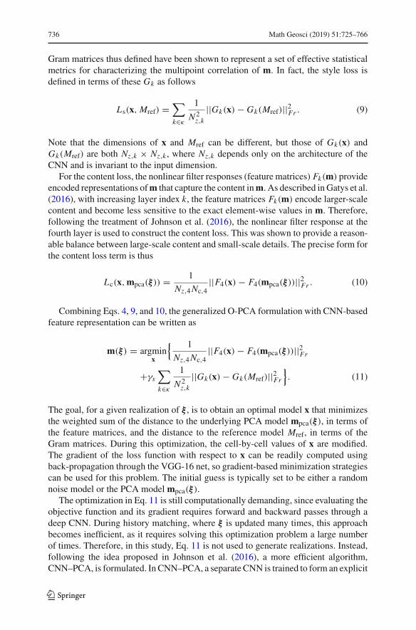
where the decision variable W denotes the parameters in the model transform net,and the loss function in Eq. 12 is the average over the training set. For each pair ofPCA and post-processed models, the loss function is the same as in Eq. 11. Note thatthe training of the model transform net is an unsupervised learning process, as thereis no pre-defined ‘true’ or ‘reference’ post-processed model provided for each PCAmodel in the training set. In Eq. 12, Gk(Mref), k ∈ κ , and F4(mi
pca), i = 1, . . . Nt,
123
738 Math Geosci (2019) 51:725–766
Fig. 5 Process for evaluating content and style losses in Eq. 12 for one pair of corresponding PCA andpost-processed models. Quantifying these losses is required to train the model transform net
can both be pre-computed and reused during the minimization, since these involve(respectively) only the training image and the PCA training realizations, which do notchange during the optimization. To reiterate, during this training procedure, the goalis to determine the parameters associated with the model transform net fW . This isin contrast to the optimization in Eq. 11, where the goal was to vary the cell-by-cellvalues of x. The current optimization (Eq. 12) does however involve quantities fromthe VGG-16 network, which is also used for Eq. 11.
Figure 5 illustrates the procedure for evaluating content and style losses, for onePCAmodel in the training set, for the binary channelized system. The PCAmodelmpcais fed through the model transform net to obtain the post-processed model fW (mpca).Next mpca, fW (mpca) and the reference model Mref are converted into a third-ordertensor of size Nx × Ny ×3, and their components are mapped to the range [0, 255], asdescribed above. These are then fed through theVGG-16 network to extract the featurematrices Fk and compute the Gram matrices Gk , k ∈ κ . In this case, the referencemodel Mref is the training image (Fig. 1) of dimensions N t
x × N ty , which is different
from the size of the models. Note that the post-processed model fW (mpca), shown inFig. 5, is obtained with the optimal model transform net.
The gradient of the objective function with respect to W can be readily computedusing back-propagation through the CNN. The adaptive moment estimation (ADAM)algorithm, which has been proven effective for optimizing various deep neural net-works, is used as the optimizer (KingmaandBa2014).ADAMrepresents one approachfor the stochastic gradient descent method. In stochastic gradient descent and its vari-ants, the gradient at each iteration is approximated using mini-batches of the trainingset rather than the entire training set at once. In other words, at each iteration, theaverage loss in Eq. 12 is evaluated over a small batch of Nb PCA models selectedfrom the training set, where Nb is the batch size. The rate at which decision variablesare updated at each iteration is controlled by the learning rate lr.
123
Math Geosci (2019) 51:725–766 739
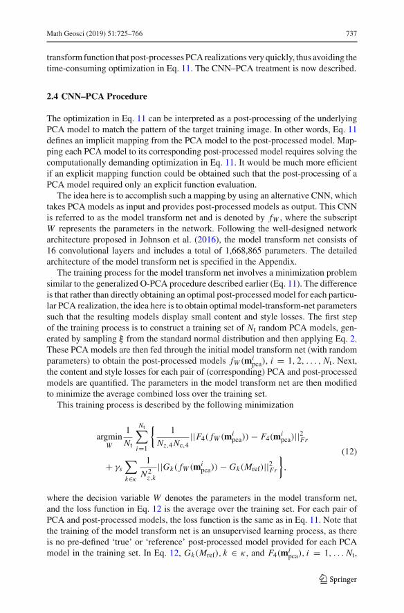
Fig. 6 Post-processing a PCA model with the model transform net and a final hard-thresholding step
After model-transform-net training, given a PCA model mpca, the post-processedmodel fW (mpca) can be obtained very quickly from a forward pass ofmpca through themodel transformnet, as shown inFig. 6.Note that the transformation through themodeltransform net is differentiable. The derivative ∂ fW (mpca)/∂mpca can be obtained usingback-propagation through the model transform net. This enables the direct calculationof ∂ fW (mpca)/∂ξ (using the chain rule and the fact that ∂mpca/∂ξ = UlΣl ). Althoughgradient-free historymatching is applied in this study (as described in Sect. 6), formoreefficient gradient-based methods, ∂ fW (mpca)/∂ξ is required. A significant advantageof this approach is that it provides the necessary derivative.
It can be seen in Fig. 6 that fW (mpca) is not strictly binary. A final histogramtransformation can be applied, if desired, to ensure that the post-processed modelsare binary or very close to binary. Since gradient-free history matching is used in thiswork, a simple non-differentiable hard-thresholding step, with a cutoff value of 0.5,is applied here. Application of a differentiable histogram transformation will preservethe differentiability of the CNN–PCA procedure. As discussed in the extension ofCNN–PCA to bimodal systems in Sect. 7, one option is to use O-PCA as a finalpost-processing step.
The overall CNN–PCA procedure is summarized in Algorithm 1. The CNN–PCAalgorithm used here is modified from an open-source implementation (Kadian 2018)of the procedure in Johnson et al. (2016) within the PyTorch Python library (Paszkeet al. 2017). In PyTorch and many other deep-learning frameworks, back-propagationthrough neural networks for computing gradients can be readily accomplished usingauto-differentiation.
2.5 Hard Data Loss
Hard data refer to measurements of static geological properties, such as the perme-ability values, at particular locations (typically at exploration and production wells).The ability to honor available hard data is an important aspect of any geologicalparameterization method. PCA and O-PCA models honor all hard data if the originalensemble of realizations used to construct the PCA representation honors these data.The deep-learning-based models in Dupont et al. (2018) and Mosser et al. (2018) uti-lize an additional loss term that penalizes discrepancies between the outputmodels andhard data. An alternative approach was proposed by Chan and Elsheikh (2018). Theytrained an inference net to sample latent variable realizations that only generate con-
123

740 Math Geosci (2019) 51:725–766
Algorithm 1: CNN–PCA Procedure
1 Construct PCA2 Generate Nr realizations of m based on a training image using the ‘snesim’
algorithm within SGeMS
3 Construct data matrix Y in Eq. 1, perform singular value decomposition of Y ,
and determine the reduced dimension l to obtain matrices Ul and Σl in Eq. 2
4 Train the model transform net5 Sample Nt random realizations of ξ from N (0, Il) and obtain Nt random PCA
models by applying Eq. 2
6 Train the model transform net fW with Eq. 12 or Eq. 13 (if hard data are
included) using the ADAM algorithm with batch size Nb and learning rate lr7 Generate new random realizations using CNN–PCA model8 Sample ξ from N (0, Il) and obtain the PCA model mpca(ξ) by applying Eq. 2
9 Feed mpca(ξ) through the trained model transform net to obtain fW (mpca(ξ)),
and apply a final histogram transformation to obtain the CNN–PCA model
mcnn(ξ)
ditional realizations (when fed to a GAN originally trained to generate unconditionalrealizations).
In this study, although the CNN–PCA modelsmcnn are post-processed frommpca,training the model transform net with Eq. 12 does not guarantee that all hard datawill be honored. To address this issue, an additional hard data loss term is introduced.This treatment is similar to that in Dupont et al. (2018) and Mosser et al. (2018). TheCNN–PCA minimization for conditional systems is now given by
argminW
1
Nt
Nt∑
i=1
{1
Nz,4Nc,4||F4( fW (mi
pca)) − F4(mipca)||2Fr
+ γs∑
k∈κ
1
N 2z,k
||Gk( fW (mipca)) − Gk(Mref)||2Fr + γh Lh
}.
(13)
Here, γh is a weighting factor, referred to as the hard data weight, for the new loss Lh.This hard data loss is given by
Lh = 1
Nh
[hT (mi
pca − fW (mipca))
2], (14)
where h ∈ RNc×1 is a hard data indicator vector, with h j = 1 meaning there are hard
data for grid block j and h j = 0 meaning there are no hard data for grid block j , thesquare difference (mi
pca − fW (mipca))
2 is evaluated component by component (to givea vector), and Nh is the number of hard data values specified. Note that this treatment
123

Math Geosci (2019) 51:725–766 741
Fig. 7 One unconditionalSGeMS realization of the binaryfacies model for the 2Dchannelized reservoir
20 40 60
10
20
30
40
50
60
0
0.2
0.4
0.6
0.8
1
for hard data loss is general and can be used for any amount and spatial distribution ofhard data. The value of γh is found through numerical experimentation. Specifically,in this study, γh is determined such that all hard data are correctly honored over a largeset of CNN–PCA models. The impact of γh will be illustrated in Sect. 4.2.
3 Model Generation Using CNN–PCA
In this and the following sections, CNN–PCA performance is assessed through avariety of evaluations. These assessments somewhat follow those presented in Vo andDurlofsky (2014), in that the (visual) quality of randomCNN–PCA realizations is firstconsidered, then static connectivity measures are presented, then flow responses for anensemble of models are assessed, and finally history matching results are evaluated. Inthe assessment in this section, CNN–PCA will be applied to generate new models forthe binary system considered in Sect. 2.1. Both unconditional and conditional modelswill be compared with O-PCA realizations. The values used for γs and γh in thissection are determined heuristically. More formal procedures for these determinationswill be described in Sect. 4.
3.1 Unconditional Realizations
Conditional realizations generated fromSGeMS, PCA, andO-PCA for a binary system(Fig. 2)were presented inSect. 2.1. The focus now is on the generation of unconditionalrealizations. The training image andmodel setup are the same as described in Sect. 2.1.A total of Nr = 1000 SGeMS unconditional realizations (Fig. 7) are generated andused to construct the PCA representation (Eq. 2), with a reduced dimension l = 70.For the O-PCA representation (Eq. 3), a weighting factor of γ = 0.8 is used (Voand Durlofsky 2014). Note that the same set of SGeMS realizations is used for PCA,O-PCA, and CNN–PCA model construction.
Figure 8 displays two random PCA model realizations and the corresponding O-PCA and CNN–PCA models. It is evident that the O-PCA models (Fig. 8b, e) displaysharper features than the corresponding PCA models (Fig. 8a, d). However, the chan-nels in the O-PCAmodels lack the degree of connectivity evident in the training image
123

742 Math Geosci (2019) 51:725–766
20 40 60
10
20
30
40
50
60
-0.5
0
0.5
1
1.5
(a)20 40 60
10
20
30
40
50
60
0
0.2
0.4
0.6
0.8
1
(b)20 40 60
10
20
30
40
50
60
0
0.2
0.4
0.6
0.8
1
(c)
20 40 60
10
20
30
40
50
60
-0.5
0
0.5
1
1.5
(d)20 40 60
10
20
30
40
50
60
0
0.2
0.4
0.6
0.8
1
(e)20 40 60
10
20
30
40
50
60
0
0.2
0.4
0.6
0.8
1
(f)
Fig. 8 Unconditional realizations for the 2D channelized facies model. a, d Two PCA realizations, b, etwo corresponding O-PCA realizations, and c, f two corresponding CNN–PCA realizations
(Fig. 1) and in the SGeMS realization (Fig. 7). In addition, the channel width in thetraining image is very consistent, while in the O-PCA realizations, large variations areevident in Fig. 8b, e. These behaviors were also observed by Vo and Durlofsky (2014).
CNN–PCA realizations are generated following Algorithm 1. The first step is totrain the model transform net. The training set consists of Nt = 3000 random PCArealizations (Eq. 2). The value of the style weight γs was investigated over a rangefrom 0.05 to 3. Based on visual inspection, a value of γs = 0.3 was found to provideCNN–PCAmodels with the best balance between resemblance to the PCAmodels andconsistency with the training image (additional values of γs are considered below andin Sect. 4). The model transform net was then trained with the ADAM algorithm for atotal of 2250 iterations, with a batch size of Nb = 4 and a learning rate of lr = 0.001.The values of these parameters were obtained through numerical experiments. Thetraining process requires around 3 minutes with one GPU (NVIDIA Tesla K80) forthis case. With the trained model transform net, new CNN–PCAmodels are generatedfollowing steps 8 and 9 in Algorithm 1.
Figure 8c, f shows the CNN–PCA realizations corresponding to the PCA real-izations in Fig. 8a, d. It is clear that the binary features and the channel width andconnectivity show significant improvement relative to the PCA and O-PCA realiza-tions. In addition, the relative locations of sand andmud in the CNN–PCA realizationsare consistent with the trends in the corresponding PCA realizations. These compari-son results demonstrate that CNN–PCA realizations can better preserve the geologicalfeatures displayed in the training image (Fig. 1). This suggests that the CNN–PCAformulation described in Sect. 2.4 is indeed able to capture higher-order spatial statis-tics.
123

Math Geosci (2019) 51:725–766 743
20 40 60
10
20
30
40
50
60
0
0.2
0.4
0.6
0.8
1
(a)20 40 60
10
20
30
40
50
60
0
0.2
0.4
0.6
0.8
1
(b)20 40 60
10
20
30
40
50
60
0
0.2
0.4
0.6
0.8
1
(c)20 40 60
10
20
30
40
50
60
0
0.2
0.4
0.6
0.8
1
(d)
Fig. 9 CNN–PCA realizations with different style weight γs. a, b γs = 0.05 and c, d γs = 3
The impact of style weight γs on CNN–PCA models is now illustrated (a quanti-tative assessment will be presented in Sect. 4). In general, small γs leads to modelsthat closely resemble the corresponding PCAmodels but display incorrect spatial cor-relation, while large γs values have the opposite effect. In addition, the variabilityin CNN–PCA realizations collapses (i.e., all of the CNN–PCA realizations becomesimilar) when using overly large γs . This is referred to as mode collapse and has beenobserved in previous deep generative models such as GAN (Arjovsky et al. 2017).These observations are apparent in Fig. 9. Realizations constructed using a small styleweight of γs = 0.05, shown in Fig. 9a, b, are basically block-wise mappings of theunderlying PCA models (Fig. 8a, d). They display relatively poor channel continuityand inconsistent channel width. With a large style weight of γs = 3, the CNN–PCArealizations do not honor the general sand and mud locations indicated in the corre-sponding PCA models. They also show less variability in terms of channel geometry.A value of γs = 0.3, used in this study, is seen to provide realizations (Fig. 8c, f) thatrepresent an appropriate balance between the two loss functions.
3.2 Conditional Realizations
The generation of CNN–PCA realizations conditioned to hard data (facies type atwell locations) is now considered. The setup is the same as that considered earlierin Sect. 2.1. The training image applied in Sect. 2.1 is again used here, and it is alsoassumed that hard data are available at 16well locations, as inVo andDurlofsky (2014).The hard data locations are indicated by the white points in Fig. 10. Three wells arelocated in mud and the other 13 wells are located in sand. Conditional models areconstructed as follows. First, Nr = 1000 conditional SGeMS realizations that honorall hard data are generated. These are used to construct the PCA representation, againwith a reduced dimension of l = 70. Then, 200 PCA realizations and correspondingO-PCA realizations are generated. As noted in Sect. 2.5, these models honor all of thehard data. The setup for training the model transform net in CNN–PCA is the same asin the previous section, except that the hard data loss function (Eqs. 13 and 14) is nowincluded. The hard data weight γh is set to 16 based on numerical experimentation andthe criterion given in Sect. 2.5. A total of 200 CNN–PCA models are then generatedby post-processing the 200 PCA realizations with the trained model transform net.
In this case, each of the 200 CNN–PCA models also honors all of the hard data.This demonstrates that the CNN–PCA procedure is able to generate conditional real-
123

744 Math Geosci (2019) 51:725–766
20 40 60
10
20
30
40
50
60
-0.5
0
0.5
1
1.5
(a)20 40 60
10
20
30
40
50
60
0
0.2
0.4
0.6
0.8
1
(b)20 40 60
10
20
30
40
50
60
0
0.2
0.4
0.6
0.8
1
(c)
20 40 60
10
20
30
40
50
60
-0.5
0
0.5
1
1.5
(d)20 40 60
10
20
30
40
50
60
0
0.2
0.4
0.6
0.8
1
(e)20 40 60
10
20
30
40
50
60
0
0.2
0.4
0.6
0.8
1
(f)
Fig. 10 Conditional realizations for the 2D channelized facies model with hard data at 16 wells. a, dTwo PCA realizations, b, e two corresponding O-PCA realizations, c, f two corresponding CNN–PCArealizations
izations for this binary system, and that the value of γh is sufficiently large. Figure 10displays two PCA realizations and the corresponding O-PCA and CNN–PCA realiza-tions. It is evident that the CNN–PCA realizations do indeed honor facies type at allwell locations. Additionally, the CNN–PCA realizations continue to display channelsinuosity and width consistent with the training image. Note finally that the O-PCArealizations in this case display better channel continuity than do those for the uncon-ditioned case (compare Figs. 10b, e to 8b, e), though the channel geometry in theCNN–PCA realizations is still closer to that in the training image.
4 Connectivity Measures and Formal Selection of Weights
In this section, a quantitative measure for channel connectivity is introduced. Thismetric is then used to assess the quality of CNN–PCA and O-PCA realizations relativeto reference SGeMS realizations. The use of this (fast to compute) static quantity forformally determining γs and γh is then described.
4.1 Connectivity Measure for Channel Continuity
In Sect. 3, the visual consistency between CNN–PCA models and SGeMS modelswas demonstrated. In this section, a metric referred to as the two-point connectivityfunction (CF) is applied to formalize this assessment. CF quantifies the proportion ofcell (pixel) pairs that are connected through a continuous sand channel. For a two-dimensional system, the connectivity function for model k is defined as
123

Math Geosci (2019) 51:725–766 745
CFkv1,v2(h) =∑Nx
i=1
∑Nyj=1 C
(mk
i, j ,mki+hv1, j+hv2
)
∑Nxi=1
∑Nyj=1 P
(mk
i, j ,mki+hv1, j+hv2
) . (15)
Here Nx and Ny are the number of grid blocks in the x and y directions, v1 andv2 indicate the direction between the cell pairs, and the lag h specifies the distancebetween the cell pairs. The denominator P counts the total number of cell pairs alongthe specified direction and distance, i.e.,
P(mki, j ,m
ki+hv1, j+hv2
) ={1 i + hv1 ≤ Nx , j + hv2 ≤ Ny,
0 otherwise.(16)
The numeratorC counts the number of cell pairs connected via continuous sand alongthe specified direction and distance
C(mki, j ,m
ki+hv1, j+hv2
) =
⎧⎪⎪⎪⎨
⎪⎪⎪⎩
1 i + hv1 ≤ Nx , j + hv2 ≤ Ny and
mki, j = mk
i+hv1, j+hv2= 1 and
mki, j ↔ mk
i+hv1, j+hv2,
0 otherwise.
(17)
Here, mki, j ↔ mk
i+hv1, j+hv2indicates that cells mk
i, j and mki+hv1, j+hv2
are connected
via continuous sand. More specifically, mki, j ↔ mk
i+hv1, j+hv2means that there exists
a sequence of connected grid blocks in the sand facies between these two cells. By‘connected’ we mean that adjacent cells in the sequence share an edge (not a corner).The connectivity function defined in Eq. 15 ismodified from the connectivity or clusterfunctions described in Torquato et al. (1988) and Pardo-Igúzquiza and Dowd (2003),in that the denominator here includes all cell pairs instead of just pairs with bothpoints in the same facies. This form was found to provide smoother curves, which isimportant for the error metric defined below.
Following the same setup as in Sect. 3.1, 200 new unconditional PCA realizationsand corresponding O-PCA and CNN–PCA realizations (with style weight γs = 0.3)are generated. In addition, 200 new unconditional SGeMS realizations are generatedas reference models. The connectivity functions in three directions, namely in thex-direction (v1 = 1, v2 = 0), the y-direction (v1 = 0, v2 = 1), and along thediagonal y = x (v1 = v2 = 1), are computed for each of these models. Because theconnectivity function considered here is strictly applicable only for binary systems,the O-PCAmodels (which have values between 0 and 1) are mapped to binary modelsusing hard thresholding, with a cutoff value of 0.5, before computing the connectivityfunction.
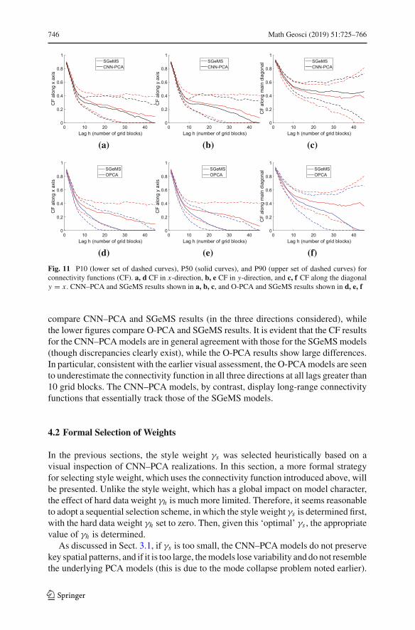
Figure 11 displays the P10, P50, and P90 results for the connectivity function forthe different sets of models. The solid curves correspond to the P50 results, and thelower and upper dashed curves to the P10 and P90 results. The P50 CF value (andsimilarly for P10 and P90 values) at a particular lag corresponds to the 50th percentile(over the 200 realizations) in the results at that value of h. The upper set of figures
123
746 Math Geosci (2019) 51:725–766
0 10 20 30 40Lag h (number of grid blocks)
0
0.2
0.4
0.6
0.8
1C
F al
ong
x ax
is
SGeMSCNN-PCA
(a)
0 10 20 30 40Lag h (number of grid blocks)
0
0.2
0.4
0.6
0.8
1
CF
alon
g y
axis
SGeMSCNN-PCA
(b)
0 10 20 30 40Lag h (number of grid blocks)
0
0.2
0.4
0.6
0.8
1
CF
alon
g m
ain
diag
onal
SGeMSCNN-PCA
(c)
0 10 20 30 40Lag h (number of grid blocks)
0
0.2
0.4
0.6
0.8
1
CF
alon
g x
axis
SGeMSOPCA
(d)
0 10 20 30 40Lag h (number of grid blocks)
0
0.2
0.4
0.6
0.8
1C
F al
ong
y ax
is
SGeMSOPCA
(e)
0 10 20 30 40Lag h (number of grid blocks)
0
0.2
0.4
0.6
0.8
1
CF
alon
g m
ain
diag
onal
SGeMSOPCA
(f)
Fig. 11 P10 (lower set of dashed curves), P50 (solid curves), and P90 (upper set of dashed curves) forconnectivity functions (CF). a, d CF in x-direction, b, e CF in y-direction, and c, f CF along the diagonaly = x . CNN–PCA and SGeMS results shown in a, b, c, and O-PCA and SGeMS results shown in d, e, f
compare CNN–PCA and SGeMS results (in the three directions considered), whilethe lower figures compare O-PCA and SGeMS results. It is evident that the CF resultsfor the CNN–PCAmodels are in general agreement with those for the SGeMSmodels(though discrepancies clearly exist), while the O-PCA results show large differences.In particular, consistent with the earlier visual assessment, the O-PCAmodels are seento underestimate the connectivity function in all three directions at all lags greater than10 grid blocks. The CNN–PCA models, by contrast, display long-range connectivityfunctions that essentially track those of the SGeMS models.
4.2 Formal Selection of Weights
In the previous sections, the style weight γs was selected heuristically based on avisual inspection of CNN–PCA realizations. In this section, a more formal strategyfor selecting style weight, which uses the connectivity function introduced above, willbe presented. Unlike the style weight, which has a global impact on model character,the effect of hard data weight γh is much more limited. Therefore, it seems reasonableto adopt a sequential selection scheme, in which the style weight γs is determined first,with the hard data weight γh set to zero. Then, given this ‘optimal’ γs , the appropriatevalue of γh is determined.
As discussed in Sect. 3.1, if γs is too small, the CNN–PCA models do not preservekey spatial patterns, and if it is too large, themodels lose variability and do not resemblethe underlying PCA models (this is due to the mode collapse problem noted earlier).
123
Math Geosci (2019) 51:725–766 747
0 10 20 30 40Lag h (number of grid blocks)
0
0.2
0.4
0.6
0.8
1C
F al
ong
mai
n di
agon
al
SGeMSCNN-PCA γs=0.01
(a)
0 10 20 30 40Lag h (number of grid blocks)
0
0.2
0.4
0.6
0.8
1
CF
alon
g m
ain
diag
onal
SGeMSCNN-PCA γs=3.0
(b)
0 0.5 1 1.5 2 2.5 3Style weight γs
0
2
4
6
8
10
12
14
ER
R fo
r CF
quan
tiles
γs=0.3
(c)
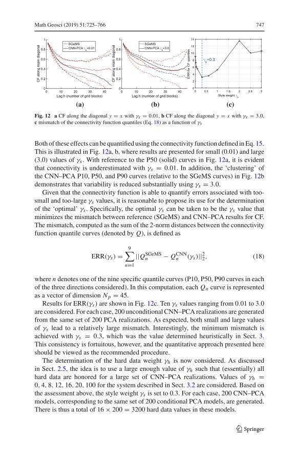
Fig. 12 a CF along the diagonal y = x with γs = 0.01, b CF along the diagonal y = x with γs = 3.0,c mismatch of the connectivity function quantiles (Eq. 18) as a function of γs
Both of these effects can be quantified using the connectivity function defined inEq. 15.This is illustrated in Fig. 12a, b, where results are presented for small (0.01) and large(3.0) values of γs . With reference to the P50 (solid) curves in Fig. 12a, it is evidentthat connectivity is underestimated with γs = 0.01. In addition, the ‘clustering’ ofthe CNN–PCA P10, P50, and P90 curves (relative to the SGeMS curves) in Fig. 12bdemonstrates that variability is reduced substantially using γs = 3.0.
Given that the connectivity function is able to quantify errors associated with too-small and too-large γs values, it is reasonable to propose its use for the determinationof the ‘optimal’ γs . Specifically, the optimal γs can be taken to be the γs value thatminimizes the mismatch between reference (SGeMS) and CNN–PCA results for CF.The mismatch, computed as the sum of the 2-norm distances between the connectivityfunction quantile curves (denoted by Q), is defined as
ERR(γs) =9∑
n=1
||QSGeMSn − QCNN
n (γs)||22, (18)
where n denotes one of the nine specific quantile curves (P10, P50, P90 curves in eachof the three directions considered). In this computation, each Qn curve is representedas a vector of dimension Np = 45.
Results for ERR(γs) are shown in Fig. 12c. Ten γs values ranging from 0.01 to 3.0are considered. For each case, 200 unconditional CNN–PCA realizations are generatedfrom the same set of 200 PCA realizations. As expected, both small and large valuesof γs lead to a relatively large mismatch. Interestingly, the minimum mismatch isachieved with γs = 0.3, which was the value determined heuristically in Sect. 3.This consistency is fortuitous, however, and the quantitative approach presented hereshould be viewed as the recommended procedure.
The determination of the hard data weight γh is now considered. As discussedin Sect. 2.5, the idea is to use a large enough value of γh such that (essentially) allhard data are honored for a large set of CNN–PCA realizations. Values of γh =0, 4, 8, 12, 16, 20, 100 for the system described in Sect. 3.2 are considered. Based onthe assessment above, the style weight γs is set to 0.3. For each case, 200 CNN–PCAmodels, corresponding to the same set of 200 conditional PCA models, are generated.There is thus a total of 16 × 200 = 3200 hard data values in these models.
123

748 Math Geosci (2019) 51:725–766
Fig. 13 Percentage of hard datamatched as a function of harddata weight γh
0 20 40 60 80 100
Hard Data Weight γh
98
98.5
99
99.5
100
Har
d D
ata
Mat
ch P
erce
ntag
e
γh=16
The percentage of hard data values preserved in the CNN–PCA models, as a func-tion of γh , is shown in Fig. 13. Since CNN–PCA models are post-processed fromconditional PCA realizations, even without the hard data loss term (i.e., γh = 0),more than 98% of the hard data are honored. As γh increases, the percentage of pre-served hard data reaches 100%. In general, it is not guaranteed that this percentagestays at exactly 100% as γh is further increased (though it is expected to be very close).In addition, if γh is taken to be very large, the variability in the CNN–PCAmodels cancollapse. This is observed in this case for γh = 1000. Therefore, it is recommendedthat the smallest γh be used such that (essentially) all hard data are correctly honoredover a large set of CNN–PCA models.
Using the procedures described in this section to determine γs and γh , multipleiterations of the training process will be required. This should not be of major con-cern, however, since the training of the CNN–PCA model transform net (the onlystep that needs to be repeated) is reasonably efficient. In addition, strategies suchas early stopping (meaning training for a relatively small number of epochs) couldbe adopted. Coarse-tuning, in which promising ranges of γs or γh are first identi-fied, and then a more refined search is performed, could also provide computationalsavings.
Although not investigated here, training the model transform net and optimiz-ing the weights is expected to be scalable to larger and more realistic geologicalmodels, for several reasons. First, the model transform net uses all convolutionallayers (see Appendix), so the number of parameters will not increase significantlyfor larger models. Second, the number of γs and γh values evaluated in weightselection is not expected to increase with larger models. Third, training and weightselection are naturally parallelizable, so elapsed time can be managed by usingmore GPUs. Finally, it is expected that the optimal values for γs and γh obtainedfor a given case will represent reasonable starting points for subsequent cases inwhich the scenario (or training image) is updated and/or more hard data becomeavailable.
123

Math Geosci (2019) 51:725–766 749
I1I2
P1
P2
20 40 60
10
20
30
40
50
60
0
0.2
0.4
0.6
0.8
1
(a)
I1I2
P1
P2
20 40 60
10
20
30
40
50
60
0
0.2
0.4
0.6
0.8
1
(b)
I1I2
P1
P2
20 40 60
10
20
30
40
50
60
0
0.2
0.4
0.6
0.8
1
(c)
Fig. 14 Random realizations conditioned to hard data at fourwell locations. a SGeMS realization,bO-PCArealization, and c corresponding CNN–PCA realization
5 Flow Simulation with Random CNN–PCA Realizations
In this section, the flow statistics (e.g., P10, P50, P90 responses) associated withan ensemble of CNN–PCA and O-PCA models are compared to those for referenceSGeMS models. Comparisons of flow responses between O-PCA and SGeMs modelswere performed by Vo and Durlofsky (2014). In that study, O-PCA was found to pro-vide flow statistics in reasonable agreement with SGeMS for models with a relativelylarge amount of conditioning data. However, in the absence of conditioning data, orwhen such data are sparse, the flow responses for O-PCA models are less accurate.Here, a conditional system with a small amount of conditioning data is considered.This is a particularly challenging case since production wells are far from injectionwells, so maintaining channel continuity in the geomodel strongly influences flowresponse.
The reservoir model is defined on a 60×60 grid. Grid blocks are of size 50 m in thex- and y-directions, and 10 m in the z-direction. The binary facies model representsa conditional channelized system, with hard data at two injection wells (I1 and I2)and two production wells (P1 and P2), as shown in Fig. 14. All four wells are locatedin sand. The same setup as in Sect. 3.2 is used to construct the PCA, O-PCA andCNN–PCA models, except the hard data weight γh for CNN–PCA is 10 in this case.A smaller γh may be required here than in the earlier example because there are fewerhard data to honor in this case. A total of 200 (new) random PCA realizations andcorresponding O-PCA and CNN–PCA realizations are generated. For the SGeMSmodels, a new set of 200 realizations generated with ‘snesim’ is used.
The binary facies modelm denotes the grid-block facies type, withmi = 1 indicat-ing sand and mi = 0 indicating mud in block i . The grid-block porosity is specifiedas φi = φsmi + φm(1 − mi ), where φs = 0.25 is the sand porosity and φm = 0.15is the mud porosity. Grid-block permeability (taken to be isotropic) is specified aski = a exp(bmi ), where the two constants are a = 2 md and b = ln 1000. This resultsin permeability values of 2000 md for sand and 2 md for mud, which correspondsto a strong contrast between facies. Note that this contrast is 10 times that in Vo andDurlofsky (2014), where permeabilities of 2000 md for sand and 20 md for mud wereused.
123
750 Math Geosci (2019) 51:725–766
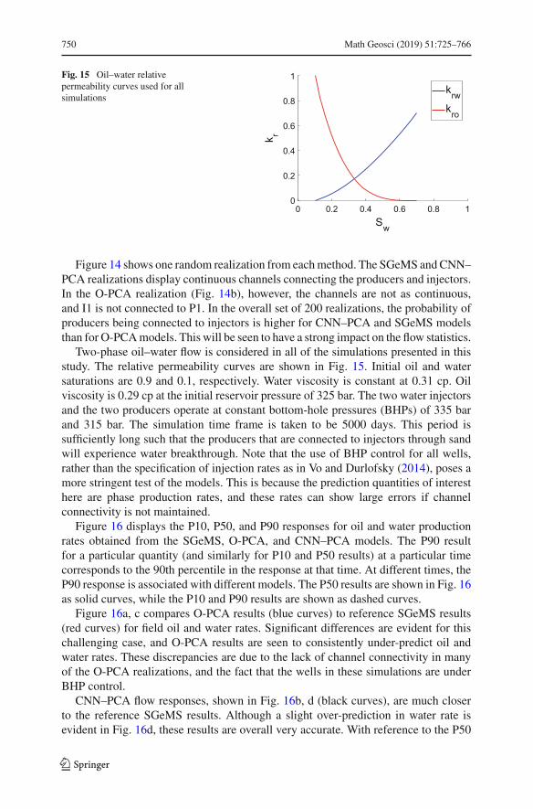
Fig. 15 Oil–water relativepermeability curves used for allsimulations
0 0.2 0.4 0.6 0.8 1Sw
0
0.2
0.4
0.6
0.8
1
k r
krwkro
Figure 14 shows one random realization from eachmethod. The SGeMS and CNN–PCA realizations display continuous channels connecting the producers and injectors.In the O-PCA realization (Fig. 14b), however, the channels are not as continuous,and I1 is not connected to P1. In the overall set of 200 realizations, the probability ofproducers being connected to injectors is higher for CNN–PCA and SGeMS modelsthan for O-PCAmodels. This will be seen to have a strong impact on the flow statistics.
Two-phase oil–water flow is considered in all of the simulations presented in thisstudy. The relative permeability curves are shown in Fig. 15. Initial oil and watersaturations are 0.9 and 0.1, respectively. Water viscosity is constant at 0.31 cp. Oilviscosity is 0.29 cp at the initial reservoir pressure of 325 bar. The two water injectorsand the two producers operate at constant bottom-hole pressures (BHPs) of 335 barand 315 bar. The simulation time frame is taken to be 5000 days. This period issufficiently long such that the producers that are connected to injectors through sandwill experience water breakthrough. Note that the use of BHP control for all wells,rather than the specification of injection rates as in Vo and Durlofsky (2014), poses amore stringent test of the models. This is because the prediction quantities of interesthere are phase production rates, and these rates can show large errors if channelconnectivity is not maintained.
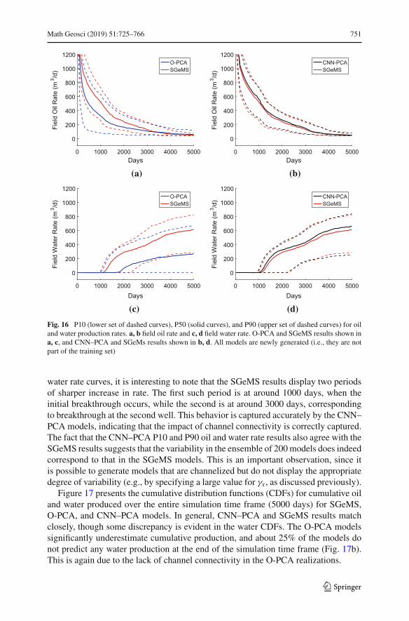
Figure 16 displays the P10, P50, and P90 responses for oil and water productionrates obtained from the SGeMS, O-PCA, and CNN–PCA models. The P90 resultfor a particular quantity (and similarly for P10 and P50 results) at a particular timecorresponds to the 90th percentile in the response at that time. At different times, theP90 response is associated with different models. The P50 results are shown in Fig. 16as solid curves, while the P10 and P90 results are shown as dashed curves.
Figure 16a, c compares O-PCA results (blue curves) to reference SGeMS results(red curves) for field oil and water rates. Significant differences are evident for thischallenging case, and O-PCA results are seen to consistently under-predict oil andwater rates. These discrepancies are due to the lack of channel connectivity in manyof the O-PCA realizations, and the fact that the wells in these simulations are underBHP control.
CNN–PCA flow responses, shown in Fig. 16b, d (black curves), are much closerto the reference SGeMS results. Although a slight over-prediction in water rate isevident in Fig. 16d, these results are overall very accurate. With reference to the P50
123
Math Geosci (2019) 51:725–766 751
0 1000 2000 3000 4000 5000Days
0
200
400
600
800
1000
1200Fi
eld
Oil
Rat
e (m
3 /d)
O-PCASGeMS
(a)
0 1000 2000 3000 4000 5000Days
0
200
400
600
800
1000
1200
Fiel
d O
il R
ate
(m3 /d
)
CNN-PCASGeMS
(b)
0 1000 2000 3000 4000 5000
Days
0
200
400
600
800
1000
1200
Fiel
d W
ater
Rat
e (m
3 /d) O-PCA
SGeMS
(c)
0 1000 2000 3000 4000 5000
Days
0
200
400
600
800
1000
1200
Fiel
d W
ater
Rat
e (m
3 /d) CNN-PCA
SGeMS
(d)
Fig. 16 P10 (lower set of dashed curves), P50 (solid curves), and P90 (upper set of dashed curves) for oiland water production rates. a, b field oil rate and c, d field water rate. O-PCA and SGeMS results shown ina, c, and CNN–PCA and SGeMs results shown in b, d. All models are newly generated (i.e., they are notpart of the training set)
water rate curves, it is interesting to note that the SGeMS results display two periodsof sharper increase in rate. The first such period is at around 1000 days, when theinitial breakthrough occurs, while the second is at around 3000 days, correspondingto breakthrough at the second well. This behavior is captured accurately by the CNN–PCA models, indicating that the impact of channel connectivity is correctly captured.The fact that the CNN–PCA P10 and P90 oil and water rate results also agree with theSGeMS results suggests that the variability in the ensemble of 200models does indeedcorrespond to that in the SGeMS models. This is an important observation, since itis possible to generate models that are channelized but do not display the appropriatedegree of variability (e.g., by specifying a large value for γs , as discussed previously).
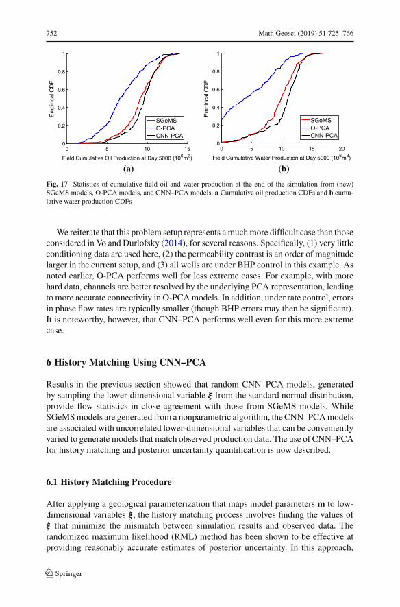
Figure 17 presents the cumulative distribution functions (CDFs) for cumulative oiland water produced over the entire simulation time frame (5000 days) for SGeMS,O-PCA, and CNN–PCA models. In general, CNN–PCA and SGeMS results matchclosely, though some discrepancy is evident in the water CDFs. The O-PCA modelssignificantly underestimate cumulative production, and about 25% of the models donot predict any water production at the end of the simulation time frame (Fig. 17b).This is again due to the lack of channel connectivity in the O-PCA realizations.
123
752 Math Geosci (2019) 51:725–766
0 5 10 15
Field Cumulative Oil Production at Day 5000 (106m3)
0
0.2
0.4
0.6
0.8
1E
mpi
rical
CD
F
SGeMSO-PCACNN-PCA
0 5 10 15 20
Field Cumulative Water Production at Day 5000 (106m3)
0
0.2
0.4
0.6
0.8
1
Em
piric
al C
DF
SGeMSO-PCACNN-PCA
(a) (b)
Fig. 17 Statistics of cumulative field oil and water production at the end of the simulation from (new)SGeMS models, O-PCA models, and CNN–PCA models. a Cumulative oil production CDFs and b cumu-lative water production CDFs
We reiterate that this problem setup represents amuchmore difficult case than thoseconsidered in Vo and Durlofsky (2014), for several reasons. Specifically, (1) very littleconditioning data are used here, (2) the permeability contrast is an order of magnitudelarger in the current setup, and (3) all wells are under BHP control in this example. Asnoted earlier, O-PCA performs well for less extreme cases. For example, with morehard data, channels are better resolved by the underlying PCA representation, leadingto more accurate connectivity in O-PCAmodels. In addition, under rate control, errorsin phase flow rates are typically smaller (though BHP errors may then be significant).It is noteworthy, however, that CNN–PCA performs well even for this more extremecase.
6 History Matching Using CNN–PCA
Results in the previous section showed that random CNN–PCA models, generatedby sampling the lower-dimensional variable ξ from the standard normal distribution,provide flow statistics in close agreement with those from SGeMS models. WhileSGeMSmodels are generated from a nonparametric algorithm, the CNN–PCAmodelsare associated with uncorrelated lower-dimensional variables that can be convenientlyvaried to generate models that match observed production data. The use of CNN–PCAfor history matching and posterior uncertainty quantification is now described.
6.1 History Matching Procedure
After applying a geological parameterization that maps model parameters m to low-dimensional variables ξ , the history matching process involves finding the values ofξ that minimize the mismatch between simulation results and observed data. Therandomized maximum likelihood (RML) method has been shown to be effective atproviding reasonably accurate estimates of posterior uncertainty. In this approach,
123
Math Geosci (2019) 51:725–766 753
multiple posterior models are obtained by performing multiple minimizations withperturbed objective functions (Kitanidis 1986; Oliver 1996).
Vo and Durlofsky (2015) provided a detailed description of RML-based subspacehistory matching for generating multiple posterior samples of ξ (and thus m). Theminimization problem is expressed as
ξ∗rml = argmin
ξ
{1
2
(d(m(ξ)) − d∗
obs
)TC−1d
(d(m(ξ)) − d∗
obs
) + 1
2
(ξ − ξ∗)T (
ξ − ξ∗)}.
(19)This objective function consists of two terms. The first term, referred to as the datamismatch, is a weighted square mismatch that quantifies the difference between simu-lated datad(m(ξ )) and (perturbed) observation datad∗
obs. Evaluatingd(m(ξ )) involvesmapping ξ to the model parameter m, which is then used to calculate reservoir prop-erties. Simulated flow responses (e.g., well rates and BHPs) at selected time pointsare then extracted to form d(m(ξ)). The measurement errors for the observed data areassumed to be independent and to follow amultivariate Gaussian distributionwith zeromean and diagonal covariance matrix Cd. In RML, the observed data are perturbedwith random noise sampled from N (0,Cd).
The second term, referred to as themodelmismatch, is a regularization term that actsto constrain ξ to be close to a random prior realization ξ∗ sampled from the standardnormal distribution.Multipleminimizations are performed, eachwith different randomrealizations of d∗
obs and ξ∗, to obtain multiple posterior models. Simulation resultsobtained from these posterior models are used to estimate the posterior uncertainty ofthe production forecast.
Note finally that in CNN–PCA, m(ξ) is given by
m(ξ) ={1, fW (UlΣlξ + m̄) ≥ 0.5,
0, fW (UlΣlξ + m̄) < 0.5,(20)
where fW represents the model transform net. Recall that the model transform net istrained in the offline process, during which weights γs and γh are determined suchthat an accurate connectivity function is recovered and hard data are consistentlyhonored. Thus, the time-consuming (offline) aspects of the CNN–PCA procedure areall completedprior to the historymatching computations. For this reason, the additionalonline cost (i.e., during history matching) of CNN–PCA relative to PCA or O-PCA isnegligible.
6.2 Problem Setup
The setup used for history matching is very similar to that considered for flow assess-ment in Sect. 5. The reservoir model is again a 2D channelized system defined on a60 × 60 grid. Here, however, the two injection wells are located around the centerof the model, as shown in Fig. 18, and the simulation time frame is only 2000 days.Injection and production well BHPs are set to 335 bar and 315 bar, respectively. Ina later stage, new production wells will be introduced in the upper-right corner of
123
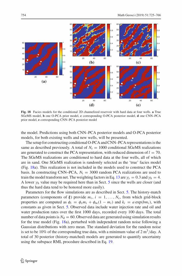
754 Math Geosci (2019) 51:725–766
I1
I2
P1
P2
20 40 60
10
20
30
40
50
60
0
0.2
0.4
0.6
0.8
1
(a)
I1
I2
P1
P2
20 40 60
10
20
30
40
50
60
0
0.2
0.4
0.6
0.8
1
(b)
I1
I2
P1
P2
20 40 60
10
20
30
40
50
60
0
0.2
0.4
0.6
0.8
1
(c)
I1
I2
P1
P2
20 40 60
10
20
30
40
50
60
0
0.2
0.4
0.6
0.8
1
(d)
I1
I2
P1
P2
20 40 60
10
20
30
40
50
60
0
0.2
0.4
0.6
0.8
1
(e)
Fig. 18 Facies models for the conditional 2D channelized reservoir with hard data at four wells. a TrueSGeMS model, b one O-PCA prior model, c corresponding O-PCA posterior model, d one CNN–PCAprior model, e corresponding CNN–PCA posterior model
the model. Predictions using both CNN–PCA posterior models and O-PCA posteriormodels, for both existing wells and new wells, will be presented.
The setup for constructing conditionalO-PCAandCNN–PCArepresentations is thesame as described previously. A total of Nr = 1000 conditional SGeMS realizationsare generated to construct the PCA representation, with reduced dimension of l = 70.The SGeMS realizations are conditioned to hard data at the four wells, all of whichare in sand. One SGeMS realization is randomly selected as the ‘true’ facies model(Fig. 18a). This realization is not included in the models used to construct the PCAbasis. In constructing CNN–PCA, Nt = 3000 random PCA realizations are used totrain themodel transform net. Theweighting factors in Eq. 13 are γs = 0.3 and γh = 4.A lower γh value may be required here than in Sect. 5 since the wells are closer (andthus the hard data tend to be honored more easily).
Parameters for the flow simulations are as described in Sect. 5. The history-matchparameters (components of ξ ) provide mi , i = 1, . . . , Nc, from which grid-blockproperties are computed as φi = φsmi + φm(1 − mi ) and ki = a exp(bmi ), withconstants as given in Sect. 5. Observed data include water injection rate and oil andwater production rates over the first 1000 days, recorded every 100 days. The totalnumber of data points is Nd = 60.Observed data are generated using simulation resultsfor the true model (Fig. 18a), perturbed with independent random noise following aGaussian distributions with zero mean. The standard deviation for the random noiseis set to be 10% of the corresponding true data, with a minimum value of 2 m3/day. Atotal of 30 posterior (history-matched) models are generated to quantify uncertaintyusing the subspace RML procedure described in Eq. 19.
123

Math Geosci (2019) 51:725–766 755
A derivative-free optimization method is applied here to solve the minimizationproblem defined in Eq. 19. This type of approach is nonintrusive with respect tothe simulator, so it can be readily used with any subsurface flow simulator. As dis-cussed in Sect. 2.4, the CNN–PCA representation is differentiable when the finalhard-thresholding step is replaced with a differentiable transformation. The algorithmcan then be applied in conjunction with efficient adjoint-gradient-based methods, aswas done with O-PCA in Vo and Durlofsky (2015).
The derivative-free optimizer used here is the hybrid PSO–MADS algorithm devel-oped by Isebor et al. (2014). This approach combines particle swarm optimization(PSO), which is a global stochastic search algorithm, with mesh adaptive direct search(MADS), a local pattern search method. By alternating between the two methods,PSO–MADS provides some amount of global exploration along with convergenceto a local minimum. This was found to be useful in field development optimizationproblems. Standalone PSO and standalone MADS have been shown to be effective inhistory matching with PCA (Echeverría Ciaurri et al. 2009; Rwechungura et al. 2011)and O-PCA (Liu 2017) parameterizations. The application of PSO–MADS for historymatching, which was found to be effective for the cases considered in this study, doesnot appear to have been reported previously.
In the example considered here, the dimension of the search space (l) is 70. A PSOswarm size of 50 is used, which means that 50 flow simulations are required at eachPSO iteration. Each MADS iteration involves evaluation of a set of stencil-based trialpoints located around the current-best solution. This entails 2l = 140 flow simulationsfor the MADS version applied here. Both PSO and MADS parallelize naturally, soif 140 compute nodes are available, the algorithm can be run fully parallelized. Theinitial guess for the minimization in Eq. 19 is set to be a random prior realization ξ∗.PSO–MADS is run in all cases for 24 iterations, which was found to provide an appro-priate level of reduction in the mismatch defined in Eq. 19. Detailed optimizer settingsand treatments were not explored here since the intent is to evaluate the general perfor-mance of CNN–PCA for history matching. Future work should assess both alternativePSO–MADS specifications and the use of adjoint-gradient-based minimization.
6.3 History Matching Results
Examples of prior and posterior (history-matched) O-PCA and CNN–PCAmodels arepresented in Fig. 18, along with the true model. The posterior models correspond tothe prior models, meaning that the ξ∗ vector associated with the prior model is usedas the initial guess in the optimization. It is evident that in the true model (Fig. 18a),high-permeability channels connect injector–producer pairs I1–P1 and I2–P2. Theseconnectivities are not fully captured in the prior models (Fig. 18b, d), but both theO-PCA and CNN–PCA posterior models (Fig. 18c, e) resolve these aspects of thesystem.
Figure 19 displayswater production results for producer P1. The vertical dashed lineat 1000 days indicates the end of the history matching period. Prior O-PCA and CNN–PCAresults are shown inFig. 19a, c, andposterior results inFig. 19b, d. It is evident thateven though the O-PCA prior results suggest that channel connectivity is insufficient
123
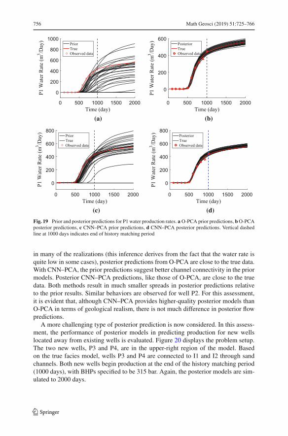
756 Math Geosci (2019) 51:725–766
0 500 1000 1500 2000Time (day)
0
200
400
600
800
1000P1
Wat
er R
ate
(m3 /D
ay)
PriorTrueObserved data
(a)
0 500 1000 1500 2000Time (day)
0
200
400
600
P1 W
ater
Rat
e (m
3 /Day
) PosteriorTrueObserved data
(b)
0 500 1000 1500 2000Time (day)
0
200
400
600
800
P1 W
ater
Rat
e (m
3 /Day
)
PriorTrueObserved data
(c)
0 500 1000 1500 2000Time (day)
0
200
400
600
800
P1 W
ater
Rat
e (m
3 /Day
) PosteriorTrueObserved data
(d)
Fig. 19 Prior and posterior predictions for P1 water production rates. aO-PCA prior predictions, bO-PCAposterior predictions, c CNN–PCA prior predictions, d CNN–PCA posterior predictions. Vertical dashedline at 1000 days indicates end of history matching period
in many of the realizations (this inference derives from the fact that the water rate isquite low in some cases), posterior predictions from O-PCA are close to the true data.With CNN–PCA, the prior predictions suggest better channel connectivity in the priormodels. Posterior CNN–PCA predictions, like those of O-PCA, are close to the truedata. Both methods result in much smaller spreads in posterior predictions relativeto the prior results. Similar behaviors are observed for well P2. For this assessment,it is evident that, although CNN–PCA provides higher-quality posterior models thanO-PCA in terms of geological realism, there is not much difference in posterior flowpredictions.
A more challenging type of posterior prediction is now considered. In this assess-ment, the performance of posterior models in predicting production for new wellslocated away from existing wells is evaluated. Figure 20 displays the problem setup.The two new wells, P3 and P4, are in the upper-right region of the model. Basedon the true facies model, wells P3 and P4 are connected to I1 and I2 through sandchannels. Both new wells begin production at the end of the history matching period(1000 days), with BHPs specified to be 315 bar. Again, the posterior models are sim-ulated to 2000 days.
123
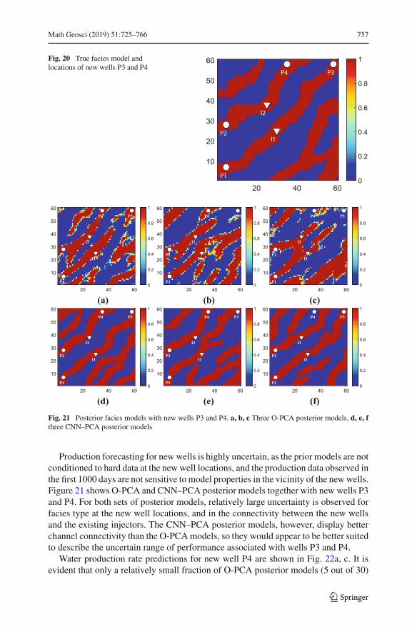
Math Geosci (2019) 51:725–766 757
Fig. 20 True facies model andlocations of new wells P3 and P4
I1
I2
P1
P2
P3P4
20 40 60
10
20
30
40
50
60
0
0.2
0.4
0.6
0.8
1
I1
I2
P1
P2
P3P4
20 40 60
10
20
30
40
50
60
0
0.2
0.4
0.6
0.8
1
(a)
I1
I2
P1
P2
P3P4
20 40 60
10
20
30
40
50
60
0
0.2
0.4
0.6
0.8
1
(b)
I1
I2
P1
P2
P3P4
20 40 60
10
20
30
40
50
60
0
0.2
0.4
0.6
0.8
1
(c)
I1
I2
P1
P2
P3P4
20 40 60
10
20
30
40
50
60
0
0.2
0.4
0.6
0.8
1
(d)
I1
I2
P1
P2
P3P4
20 40 60
10
20
30
40
50
60
0
0.2
0.4
0.6
0.8
1
(e)
I1
I2
P1
P2
P3P4
20 40 60
10
20
30
40
50
60
0
0.2
0.4
0.6
0.8
1
(f)
Fig. 21 Posterior facies models with new wells P3 and P4. a, b, c Three O-PCA posterior models, d, e, fthree CNN–PCA posterior models
Production forecasting for newwells is highly uncertain, as the prior models are notconditioned to hard data at the newwell locations, and the production data observed inthe first 1000 days are not sensitive to model properties in the vicinity of the newwells.Figure 21 shows O-PCA and CNN–PCA posterior models together with new wells P3and P4. For both sets of posterior models, relatively large uncertainty is observed forfacies type at the new well locations, and in the connectivity between the new wellsand the existing injectors. The CNN–PCA posterior models, however, display betterchannel connectivity than the O-PCAmodels, so they would appear to be better suitedto describe the uncertain range of performance associated with wells P3 and P4.
Water production rate predictions for new well P4 are shown in Fig. 22a, c. It isevident that only a relatively small fraction of O-PCA posterior models (5 out of 30)
123
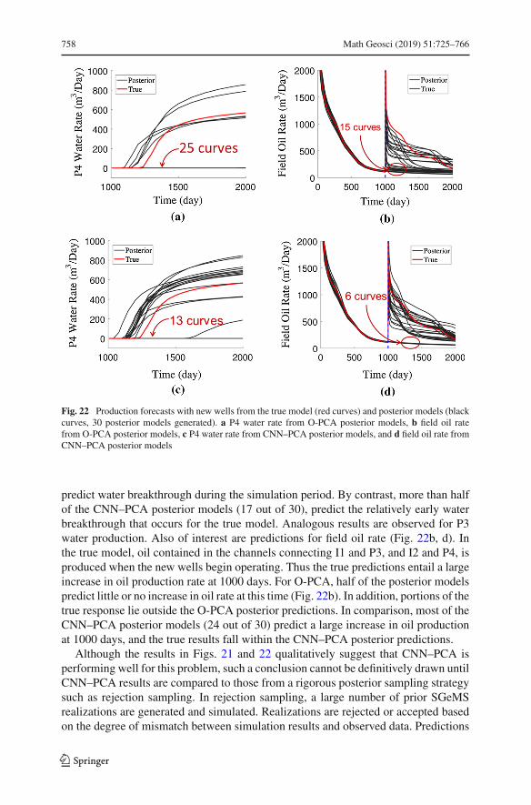
758 Math Geosci (2019) 51:725–766
Fig. 22 Production forecasts with new wells from the true model (red curves) and posterior models (blackcurves, 30 posterior models generated). a P4 water rate from O-PCA posterior models, b field oil ratefrom O-PCA posterior models, c P4 water rate from CNN–PCA posterior models, and d field oil rate fromCNN–PCA posterior models
predict water breakthrough during the simulation period. By contrast, more than halfof the CNN–PCA posterior models (17 out of 30), predict the relatively early waterbreakthrough that occurs for the true model. Analogous results are observed for P3water production. Also of interest are predictions for field oil rate (Fig. 22b, d). Inthe true model, oil contained in the channels connecting I1 and P3, and I2 and P4, isproduced when the new wells begin operating. Thus the true predictions entail a largeincrease in oil production rate at 1000 days. For O-PCA, half of the posterior modelspredict little or no increase in oil rate at this time (Fig. 22b). In addition, portions of thetrue response lie outside the O-PCA posterior predictions. In comparison, most of theCNN–PCA posterior models (24 out of 30) predict a large increase in oil productionat 1000 days, and the true results fall within the CNN–PCA posterior predictions.
Although the results in Figs. 21 and 22 qualitatively suggest that CNN–PCA isperforming well for this problem, such a conclusion cannot be definitively drawn untilCNN–PCA results are compared to those from a rigorous posterior sampling strategysuch as rejection sampling. In rejection sampling, a large number of prior SGeMSrealizations are generated and simulated. Realizations are rejected or accepted basedon the degree of mismatch between simulation results and observed data. Predictions
123

Math Geosci (2019) 51:725–766 759
50 100 150 200 250
50
100
150
200
250
0
0.2
0.4
0.6
0.8
1
(a)0 20 40 60 80 100 120
20
40
60
80
100
120
0
0.5
1
1.5
2
2.5
3
(b)0 20 40 60 80 100 120
20
40
60
80
100
120
0
0.5
1
1.5
2
2.5
3
3.5
4
(c)
Fig. 23 Input for the ‘snesim’ algorithm to generate a binary facies model for the deltaic fan system. aTraining image, b local affinity transformation region, c local rotation region
from the accepted realizations provide an accurate assessment of posterior uncertainty.Rejection sampling is extremely expensive, however, and is thus not performed in thisstudy.
7 CNN–PCA for Bimodal Deltaic Fan Systems
In this section, the CNN–PCA procedure is extended for application to a more com-plex bimodal deltaic fan system. The development is limited to the generation ofrealizations—no flow results will be presented. The model here corresponds to a non-stationary random field with global trends in channel direction and channel width.Thus, the spatial correlation structure of the deltaic fan model is more difficult tocharacterize than in the channelized case. In addition, this system is bimodal ratherthan binary, meaning that the properties within each of the facies are not constant, andinstead follow prescribed (Gaussian) distributions.
In this case, the model is defined on a 120 × 120 grid and the components of mrepresent log-permeability (log k) in each grid block. The procedure for generatingrealizations for the deltaic fan system using SGeMS is described in Vo and Durlofsky(2016). The first step is to generate a binary facies model using the ‘snesim’ algorithmwith local affinity transformation and rotation. Figure 23 shows the training imageand local regions for affinity transformation and rotation. The training image, definedon a 250 × 250 grid, represents a binary channelized system, with the main channelorientation in the y-direction. The scaling factors for the four affinity transformationregions are 1.5, 1, 0.5, and 0.3. The rotation angles for the five rotation regions are− 45◦,− 30◦, 0◦, 30◦, and 45◦. In the next step, Gaussian realizations for log k withineach facies (with mean and variance of 8 and 0.8 in sand, and 3 and 0.4 in mud) aresimulated independently using the ‘sgsim’ algorithm in SGeMS. The log-permeabilityfor each block is then assigned according to the binary facies model using the cookie-cutter approach.
A total of Nr = 1500 realizations, conditioned to hard data at 20 well locations,are generated. Figure 24 shows two SGeMS realizations and the corresponding his-tograms. The six wells toward the lower-left and lower-right portions of the model arein mud, while the other 14 wells are in sand. A PCA representation, with l = 150, is
123
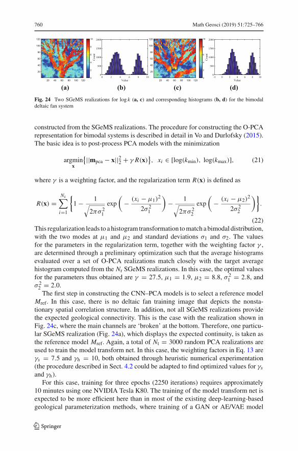
760 Math Geosci (2019) 51:725–766
20 40 60 80 100 120
20
40
60
80
100
120
0
2
4
6
8
10
(a)
0 2 4 6 8 10Value
0
500
1000
1500
2000
Cou
nt(b)
20 40 60 80 100 120
20
40
60
80
100
120
0
2
4
6
8
10
(c)
-2 0 2 4 6 8 10Value
0
500
1000
1500
2000
Cou
nt
(d)
Fig. 24 Two SGeMS realizations for log k (a, c) and corresponding histograms (b, d) for the bimodaldeltaic fan system
constructed from the SGeMS realizations. The procedure for constructing the O-PCArepresentation for bimodal systems is described in detail in Vo and Durlofsky (2015).The basic idea is to post-process PCA models with the minimization
argminx
{||mpca − x||22 + γ R(x)}, xi ∈ [log(kmin), log(kmax)], (21)
where γ is a weighting factor, and the regularization term R(x) is defined as
R(x) =Nc∑
i=1
{1 − 1
√2πσ 2
1
exp
(− (xi − μ1)
2
2σ 21
)− 1
√2πσ 2
2
exp
(− (xi − μ2)
2
2σ 22
)}.
(22)This regularization leads to a histogram transformation tomatch a bimodal distribution,with the two modes at μ1 and μ2 and standard deviations σ1 and σ2. The valuesfor the parameters in the regularization term, together with the weighting factor γ ,are determined through a preliminary optimization such that the average histogramsevaluated over a set of O-PCA realizations match closely with the target averagehistogram computed from the Nr SGeMS realizations. In this case, the optimal valuesfor the parameters thus obtained are γ = 27.5, μ1 = 1.9, μ2 = 8.8, σ 2
1 = 2.8, andσ 22 = 2.0.The first step in constructing the CNN–PCA models is to select a reference model
Mref. In this case, there is no deltaic fan training image that depicts the nonsta-tionary spatial correlation structure. In addition, not all SGeMS realizations providethe expected geological connectivity. This is the case with the realization shown inFig. 24c, where the main channels are ‘broken’ at the bottom. Therefore, one particu-lar SGeMS realization (Fig. 24a), which displays the expected continuity, is taken asthe reference model Mref. Again, a total of Nt = 3000 random PCA realizations areused to train the model transform net. In this case, the weighting factors in Eq. 13 areγs = 7.5 and γh = 10, both obtained through heuristic numerical experimentation(the procedure described in Sect. 4.2 could be adapted to find optimized values for γsand γh).
For this case, training for three epochs (2250 iterations) requires approximately10 minutes using one NVIDIA Tesla K80. The training of the model transform net isexpected to be more efficient here than in most of the existing deep-learning-basedgeological parameterization methods, where training of a GAN or AE/VAE model
123
Math Geosci (2019) 51:725–766 761
typically required more than an hour. For example, in Laloy et al. (2017, 2018),training entailed hours for 2D models of similar size as the deltaic fan case consideredhere (13 hours for the 100 × 100 model in Laloy et al. (2017) and 6 hours for the129 × 129 model in Laloy et al. (2018)) on one GPU (NVIDIA Tesla K40). Sincedifferent GPUs are used between studies, wall-clock-time comparisons are not exact,though conclusions regarding relative computational requirements may still be validgiven the large difference in training time.
The improved performance here is mainly due to the relatively small number ofepochs required for training the model transform net. Faster convergence for CNN–PCAmay be related to the fact that themodel transform net is trained to learn a simplertransformation, namely that from PCA models to CNN–PCA models, in contrast tomore complex transformations involving low-dimensional latent variables. In addition,in the previous studies, either an encoder network or a discriminator network neededto be trained to capture the multiple-point correlations of the models. In this study,an off-the-shelf network (the VGG-16 network) is used directly to characterize themultipoint statistics, which leads to additional savings.
It was found that even after appropriate training, there was still some discrep-ancy between the histogram of the models fW (mpca) and the target histogram fromthe SGeMS models. Therefore, a final histogram transformation step is performedby applying O-PCA to post-process fW (mpca). The final CNN–PCA model for thebimodal system is (analogous to Eq. 21)
mcnn = argminx
{|| fW (mpca) − x||22 + γ R(x)}, xi ∈ [log(kmin), log(kmax)], (23)
where the regularization term R(x) is defined in Eq. 22. A separate preliminary opti-mization was performed to obtain the values for γ and the parameters in R(x). Thesevalues were found to be γ = 14.7,μ1 = 2.9,μ2 = 8.3, σ 2
1 = 4.1, and σ 22 = 1.8. Note
that, using this O-PCA post-processing as the final step, the CNN–PCA procedure isdifferentiable and can thus be used with gradient-based history matching.
Figure 25 displays a new PCA realization and the corresponding O-PCA and CNN–PCA realizations, along with the histograms for the three models. The nonstationaryfeatures, including decreasing channel width with increasing y and the fan-shapedchannel structure, are honored to varying extents in the three realizations. Both theO-PCA and CNN–PCA models have bimodal histograms, while the PCA model hasan essentially Gaussian histogram. In terms of channel continuity, the CNN–PCArealization appears more consistent with the reference SGeMS model (in Fig. 24)than the PCA and O-PCA realizations for both large channels near the bottom ofthe domain and smaller channels towards the top. In addition, the spurious channelspresent in the lower-left and lower-right portions of the PCA and O-PCA modelsdo not appear in the CNN–PCA model. This demonstrates that CNN–PCA can beapplied for the bimodal nonstationary deltaic fan system. Flow results and historymatching for this and other complicated geological systemswill be considered in futurework.
123

762 Math Geosci (2019) 51:725–766
20 40 60 80 100 120
20
40
60
80
100
120
0
2
4
6
8
10
(a)20 40 60 80 100 120
20
40
60
80
100
120
0
2
4
6
8
10
(b)20 40 60 80 100 120
20
40
60
80
100
120
0
2
4
6
8
10
(c)
-5 0 5 10 15
Value
0
500
1000
1500
2000
Cou
nt
(d)
0 2 4 6 8 10
Value
0
500
1000
1500
2000
Cou
nt
(e)
0 2 4 6 8 10
Value
0
500
1000
1500
2000
Cou
nt
(f)
Fig. 25 Random conditional realizations for bimodal deltaic fan system with hard data at 20 wells. a, dPCA realization from evaluation set and histogram, b, e corresponding O-PCA realization and histogram,c, f corresponding CNN–PCA realization and histogram
8 Concluding Remarks
In this paper, a deep-learning-based approach, referred to as CNN–PCA, was devel-oped for the low-dimensional parameterization of geological models characterizedby multipoint spatial statistics. CNN–PCA represents a generalization of the O-PCAmethod, as both procedures are based on the post-processing of PCAmodels to matchthe style of a reference model. CNN–PCA utilizes a set of metrics based on a pre-trained convolutional neural network to characterizemultiple point correlations, whichenables themethod to preserve the complex geological patterns present in the referencemodel (e.g., training image). A hard data loss termwas applied to generate conditionalCNN–PCA realizations. For the 2D systems considered in this study, CNN–PCA isessentially a direct application of the fast neural style transfer algorithm originallydeveloped in computer vision for dealing with images. In CNN–PCA, the PCA mod-els are post-processed quickly by feeding them through a convolutional neural networkcalled the model transform net. The computational cost of CNN–PCA is mainly asso-ciated with the offline training of this model transform net. The training process withCNN–PCA appears to be faster than with existing deep-learning-based geologicalparameterization techniques.
Model realizations generated using CNN–PCA were presented for a 2D binarychannelized system. Even in the absence of hard data, unconditional CNN–PCArealizations provided a high level of channel continuity and uniform channel width,consistent with the reference training image. Unconditional O-PCA realizations, bycontrast, do not provide the same degree of geological realism. For conditional sys-tems, CNN–PCA models were shown to honor all hard data for the cases considered.Application of CNN–PCA for a nonstationary bimodal deltaic fan system was also
123
Math Geosci (2019) 51:725–766 763
presented. For this system, O-PCA was used as a final post-processing step to ensurethat the histogram of the final model matched the reference histogram. The CNN–PCArealizations for the bimodal deltaic fan systemwere shown to preserve the global trendsin channel direction and channel width.
A connectivity function was introduced to enable quantitative assessments of chan-nel (sand) continuity in the O-PCA and CNN–PCAmodels relative to that in referenceSGeMS models. P10, P50, and P90 results for this metric, computed in three differentdirections, were generated for unconditional O-PCA, CNN–PCA, and SGeMS real-izations. CNN–PCA was shown to provide connectivity functions in reasonably closeagreement with SGeMS connectivity functions, in contrast to those from O-PCA.It was shown that for the binary channelized system, by minimizing the mismatchbetween CNN–PCA and SGeMS connectivity results, an ‘optimal’ style weight couldbe determined in a relatively efficient manner. A technique for determining an appro-priate value for hard data weight was also described and illustrated.
The consistency betweenCNN–PCAmodels and referenceSGeMSmodelswas fur-ther demonstrated by evaluating flow-response statistics for an oil–water two-phaseflow problem. P10, P50, and P90 results and CDFs for production quantities, obtainedfrom random SGeMS, O-PCA, and CNN–PCA realizations, were compared. CNN–PCA models were shown to provide flow statistics in close agreement with flowstatistics obtained from reference SGeMS models for a challenging case involvinga small amount of conditioning data (O-PCA is not as well suited for cases that lackhard data). History matching for a conditional binary channelized system was alsoconsidered. A derivative-free optimization method, PSO–MADS, was applied for therequired minimization, and multiple posterior models were generated using a sub-space RML procedure. Both CNN–PCA and O-PCA achieved significant uncertaintyreduction for production forecasts involving existing wells, but CNN–PCAwas shownto provide more realistic results than O-PCA for forecasts involving new wells.
In this study, CNN–PCA was applied for 2D systems. In future work, extensionsto treat 3D systems are planned. For 3D cases, the off-the-shelf VGG-16 CNN, whichwas pre-trained with 2D images, is no longer directly applicable. However, the generalapproach of using convolutional neural networks to characterize complex (multipoint)3D geological models should still be valid. In fact, a 3D convolutional neural networktrained on video data sets could potentially be used to capture multipoint statisticsin 3D geological models (Tran et al. 2015). If correlations are weak in the verticaldirection, straightforward extensions of the methodology presented in this paper maybe sufficient. It is important to note that the approaches developed here, including theprocedure to determine optimal style and hard data weights, can be readily extendedto 3D models. For example, in 3D cases, hard data may derive from horizontal (ordeviated) wells, but the hard data treatment applied here will still be valid.
Other areas for future research include the evaluation of different approaches forhistory matching with CNN–PCA models. Additional minimization algorithms, suchas adjoint-gradient-based methods, as well as ensemble-based techniques, should beassessed. Multilevel history matching treatments along the lines of those presented inLiu (2017) should also be considered for use with CNN–PCA. Such methods enablehistory matching to be accomplished more efficiently in stages, using sequential setsof PCA basis components, and were shown to be effective when applied with O-PCA.
123
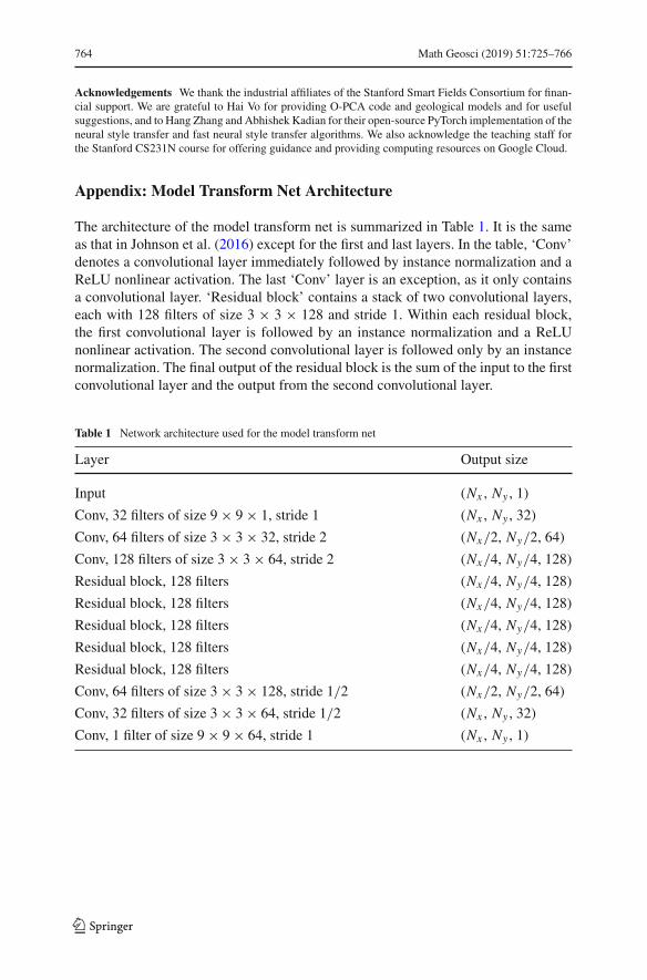
764 Math Geosci (2019) 51:725–766
Acknowledgements We thank the industrial affiliates of the Stanford Smart Fields Consortium for finan-cial support. We are grateful to Hai Vo for providing O-PCA code and geological models and for usefulsuggestions, and to Hang Zhang and Abhishek Kadian for their open-source PyTorch implementation of theneural style transfer and fast neural style transfer algorithms. We also acknowledge the teaching staff forthe Stanford CS231N course for offering guidance and providing computing resources on Google Cloud.
Appendix: Model Transform Net Architecture
The architecture of the model transform net is summarized in Table 1. It is the sameas that in Johnson et al. (2016) except for the first and last layers. In the table, ‘Conv’denotes a convolutional layer immediately followed by instance normalization and aReLU nonlinear activation. The last ‘Conv’ layer is an exception, as it only containsa convolutional layer. ‘Residual block’ contains a stack of two convolutional layers,each with 128 filters of size 3 × 3 × 128 and stride 1. Within each residual block,the first convolutional layer is followed by an instance normalization and a ReLUnonlinear activation. The second convolutional layer is followed only by an instancenormalization. The final output of the residual block is the sum of the input to the firstconvolutional layer and the output from the second convolutional layer.
Table 1 Network architecture used for the model transform net
Layer Output size
Input (Nx , Ny , 1)
Conv, 32 filters of size 9 × 9 × 1, stride 1 (Nx , Ny , 32)
Conv, 64 filters of size 3 × 3 × 32, stride 2 (Nx/2, Ny/2, 64)
Conv, 128 filters of size 3 × 3 × 64, stride 2 (Nx/4, Ny/4, 128)
Residual block, 128 filters (Nx/4, Ny/4, 128)
Residual block, 128 filters (Nx/4, Ny/4, 128)
Residual block, 128 filters (Nx/4, Ny/4, 128)
Residual block, 128 filters (Nx/4, Ny/4, 128)
Residual block, 128 filters (Nx/4, Ny/4, 128)
Conv, 64 filters of size 3 × 3 × 128, stride 1/2 (Nx/2, Ny/2, 64)
Conv, 32 filters of size 3 × 3 × 64, stride 1/2 (Nx , Ny , 32)
Conv, 1 filter of size 9 × 9 × 64, stride 1 (Nx , Ny , 1)
123

Math Geosci (2019) 51:725–766 765
References
Arjovsky M, Chintala S, Bottou L (2017) Wasserstein generative adversarial networks. Paper presented atthe 34th international conference on machine learning, Sydney, Australia, 6–11 August, pp 214–223
Astrakova A, Oliver DS (2015) Conditioning truncated pluri-Gaussian models to facies observations inensemble-Kalman-based data assimilation. Math Geosci 47(47):345–367
Canchumuni SA, Emerick AA, Pacheco MA (2017) Integration of ensemble data assimilation and deeplearning for history matching facies models. Paper OTC-28015-MS, presented at the OTC Brasil, Riode Janeiro, Brazil, 24–26 October
Canchumuni SA, Emerick AA, Pacheco M (2018) History matching channelized facies models usingensemble smoother with a deep learning parameterization. Paper presented at the 15th Europeanconference on the mathematics of oil recovery, Barcelona, Spain, 3–6 September
Chan S, Elsheikh AH (2017) Parametrization and generation of geological models with generative adver-sarial networks. arXiv preprint arXiv:1708.01810
Chan S, Elsheikh AH (2018) Parametric generation of conditional geological realizations using generativeneural networks. arXiv preprint arXiv:1807.05207
Chang H, Zhang D, Lu Z (2010) History matching of facies distribution with the EnKF and level setparameterization. J Comput Phys 229(20):8011–8030
Chen C, GaoG, Ramirez BA, Vink JC, Girardi AM (2016) Assisted historymatching of channelizedmodelsby use of pluri-principal-component analysis. SPE J 21(05):1793–1812
Deng J, Dong W, Socher R, Li LJ, Li K, Li FF (2009) ImageNet: a large-scale hierarchical image database.In: 2009 IEEE conference on computer vision and pattern recognition, IEEE, pp 248–255
Dimitrakopoulos R, Mustapha H, Gloaguen E (2010) High-order statistics of spatial random fields: explor-ing spatial cumulants for modeling complex non-Gaussian and non-linear phenomena. Math Geosci42(1):65–99
Dupont E, Zhang T, Tilke P, Liang L, BaileyW (2018) Generating realistic geology conditioned on physicalmeasurements with generative adversarial networks. arXiv preprint arXiv:1802.03065
Echeverría Ciaurri D, Mukerji T, Santos ET (2009) Robust scheme for inversion of seismic and productiondata for reservoir facies modeling. Paper SEG-2009-2432, presented at the SEG annual meeting,Houston, Texas, 25–30 October
Emerick AA (2016) Investigation on principal component analysis parameterizations for history matchingchannelized facies models with ensemble-based data assimilation. Math Geosci 49(1):85–120
Gatys LA, Ecker AS, BethgeM (2015) Texture synthesis using convolutional neural networks. In: Advancesin neural information processing systems, pp 262–270
Gatys LA, Ecker AS, Bethge M (2016) Image style transfer using convolutional neural networks. In:Proceedings of the IEEE conference on computer vision and pattern recognition, pp 2414–2423
Goodfellow I, Bengio Y, Courville A (2016) Deep learning. MIT Press, CambridgeHakim-Elahi S, Jafarpour B (2017) A distance transform for continuous parameterization of discrete geo-
logic facies for subsurface flow model calibration. Water Resour Res 53(10):8226–8249Insuasty E, Van den Hof PMJ, Weiland S, Jansen JD (2017) Low-dimensional tensor representations for
the estimation of petrophysical reservoir parameters. Paper SPE-182707-MS presented at the SPEReservoir Simulation Conference, Montgomery, Texas, 20–22 February
Isebor OJ, Echeverría Ciaurri D, Durlofsky LJ (2014) Generalized field-development optimization withderivative-free procedures. SPE J 19(05):891–908
Jafarpour B, Goyal VK, McLaughlin DB, Freeman WT (2010) Compressed history matching: exploitingtransform-domain sparsity for regularization of nonlinear dynamic data integration problems. MathGeosci 42(1):1–27
Johnson J, Alahi A, Li FF (2016) Perceptual losses for real-time style transfer and super-resolution. In:European conference on computer vision, pp 694–711
Kadian A (2018) Pytorch implementation of an algorithm for artistic style transfer. https://github.com/abhiskk/fast-neural-style/commits/master. Accessed 1 May 2018
Kingma DP, Ba J (2014) Adam: a method for stochastic optimization. arXiv preprint arXiv:1412.6980.Accessed 1 May 2018
Kitanidis PK (1986) Parameter uncertainty in estimation of spatial functions: Bayesian analysis. WaterResour Res 22(4):499–507
Laloy E, Hérault R, Lee J, Jacques D, Linde N (2017) Inversion using a new low-dimensional representationof complex binary geological media based on a deep neural network. AdvWater Resour 110:387–405
123
766 Math Geosci (2019) 51:725–766
Laloy E, Hérault R, Jacques D, Linde N (2018) Training-image based geostatistical inversion using a spatialgenerative adversarial neural network. Water Resour Res 54(1):381–406
Liu Y (2017) Multilevel strategy for O-PCA-based history matching using mesh adaptive direct search.Master’s thesis, Stanford University
Lu P,HorneRN (2000)Amultiresolution approach to reservoir parameter estimation usingwavelet analysis.Paper SPE-62985-MS, presented at the SPE annual technical conference and exhibition, Dallas, TX,1–4 October
Mosser L, Dubrule O, Blunt MJ (2017) Reconstruction of three-dimensional porous media using generativeadversarial neural networks. Phys Rev E 96(4):043,309
Mosser L, Dubrule O, Blunt MJ (2018) Conditioning of three-dimensional generative adversarial networksfor pore and reservoir-scale models. arXiv preprint arXiv:1802.05622
Oliver DS (1996) Multiple realizations of the permeability field from well test data. SPE J 1(2):145–154Pardo-Igúzquiza E, Dowd PA (2003) CONNEC3D: a computer program for connectivity analysis of 3D
random set models. Comput Geosci 29(6):775–785Paszke A, Gross S, Chintala S, Chanan G, Yang E (2017) Automatic differentiation in PyTorch. NIPS 2017
workshopPing J, Zhang D (2013) History matching of fracture distributions by ensemble Kalman filter combined
with vector based level set parameterization. J Pet Sci Eng 108:288–303Remy N, Boucher A,Wu J (2009) Applied geostatistics with SGeMS: a user’s guide. Cambridge University
Press, CambridgeReynolds AC, He N, Chu L, Oliver DS (1996) Reparameterization techniques for generating reservoir
descriptions conditioned to variograms and well-test pressure data. SPE J 1(4):413–426Rwechungura R, DadashpourM, Kleppe J (2011) Application of particle swarm optimization for parameter
estimation integrating production and time lapse seismic data. Paper SPE-146199-MS, presented atthe SPE offshore Europe conference and exhibition, Aberdeen, UK, 6–8 September
Sarma P, Durlofsky LJ, Aziz K, Chen WH (2006) Efficient real-time reservoir management using adjoint-based optimal control and model updating. Comput Geosci 10(1):3–36
Sarma P, Durlofsky LJ, Aziz K (2008) Kernel principal component analysis for efficient, differentiableparameterization of multipoint geostatistics. Math Geosci 40(1):3–32
Simonyan K, Zisserman A (2015) Very deep convolutional networks for large-scale image recognition.arXiv preprint arXiv:1409.1556
Strebelle S (2002) Conditional simulation of complex geological structures using multiple-point statistics.Math Geol 34(1):1–21
Tavakoli R, Reynolds AC (2010) History matching with parametrization based on the SVD of a dimension-less sensitivity matrix. SPE J 15(02):495–508
Torquato S, Beasley JD, Chiew YC (1988) Two-point cluster function for continuum percolation. J ChemPhys 88(10):6540–6547
Tran D, Bourdev L, Fergus R, Torresani L, Paluri M (2015) Learning spatiotemporal features with 3Dconvolutional networks. Paper presented at the 2015 IEEE international conference on computervision, Santiago, Chile, 13–16 December, pp 4489–4497
Vo HX, Durlofsky LJ (2014) A new differentiable parameterization based on principal component analysisfor the low-dimensional representation of complex geological models. Math Geosci 46(7):775–813
Vo HX, Durlofsky LJ (2015) Data assimilation and uncertainty assessment for complex geological modelsusing a new PCA-based parameterization. Comput Geosci 19(4):747–767
Vo HX, Durlofsky LJ (2016) Regularized kernel PCA for the efficient parameterization of complex geo-logical models. J Comput Phys 322:859–881
Wang Y, Arns CH, Rahman SS, Arns JY (2018) Porous structure reconstruction using convolutional neuralnetworks. Math Geosci 50(7):781–799
Zhang T, Switzer P, Journel A (2006) Filter-based classification of training image patterns for spatialsimulation. Math Geol 38(1):63–80
123