a decision support system for goods distribution …...distribution planning in urban areas. the...
TRANSCRIPT
A decision support system for goods distribution
planning in urban areas
A Thesis
In
The Department
of
Concordia Institute for Information Systems Engineering (CIISE)
Presented in Partial Fulfillment of the Requirements for the Degree of
Master of Applied Science (Quality Systems Engineering) at
Concordia University
Montreal, Quebec, Canada
April 2012
© Ali Khabbazian, 2012
CONCORDIA UNIVERSITY

School of Graduate Studies
This is to certify that the thesis prepared
By: Ali Khabbazian
Entitled: A decision support system for goods distribution planning in urban areas
and submitted in partial fulfillment of the requirements for the degree of
Master of Applied Science (Quality Systems Engineering)
complies with the regulations of the University and meets the accepted standards with
respect to originality and quality.
Signed by the final examining committee:
Andrea Schiffauerova (Chair)
Masoumeh Kazemi (External Examiner)
Zhigang Tian (Internal Examiner)
Anjali Awasthi (Supervisor)
Approved by _
Chair of Department or Graduate Program Director
____ 20 _
Dean of Faculty

iii
ABSTRACT
A decision support system for goods distribution planning in urban areas
Ali Khabbazian
Efficient goods distribution planning is vital to ensure high business revenues for logistics
operators and minimize negative impacts on the environment. In this thesis, we address three
main problems related to goods distribution planning in urban areas namely customer allocation,
order scheduling, and vehicle routing. A three step approach is proposed. In the first step, we
use Nearest Neighbour and Tabu Search for balanced allocation of customers to logistics depots.
In the second step, Genetic Algorithm approach is used to perform order scheduling at each
depot for the allocated customers. In the third and the last step, we perform vehicle allocations
and generate fastest paths for goods delivery to customers using modified Dijkstra’s algorithm.
All these decisions are made considering realistic conditions associated with goods distribution
in urban areas such as presence of congestion, municipal regulations, for example vehicle sizing,
timing and access regulations etc. The objective is to minimize total distribution costs of logistics
operators under these constraints.
A prototype decision support system is developed integrating the proposed approaches for goods
distribution planning in urban areas. The strength of the proposed decision support system is its
ability to generate fast and efficient solutions for balanced customer allocation, dynamic order
scheduling, vehicle allocation considering environmental constraints and fastest path generation
under dynamic traffic conditions. The proposed model results are verified and validated against
other standard approaches available in literature.

iv
Dedication
I dedicate my work to my devoted wife Atena, whose generosity and support has been constant
and unconditional throughout this process, and whose love and commitment to our little one,
Artan, has been a constant source of encouragement. I also dedicate this work to my always
loving family, my patient parents, my lovely son Artan and my brother-in-law Hamid, he has
been the perfect role model for me.

v
Acknowledgements
I would like to express my deep and sincere gratitude to my supervisor, Professor Anjali
Awasthi. Her wide knowledge and her logical way of thinking have been of great value for me.
Her understanding, encouragement and personal guidance have provided a good basis for the
presented thesis.
She has always dedicated her time in research. Not only has she taught me and trained me how to
be a good researcher, but she has also shown me how to utilize my time efficiently to get to my
expected goal. Furthermore, she is a very understanding and patient professor. She has always
put me in the right direction. Most importantly, I will forever consider her as my greatest
advisor.
I owe my thanks to my always-loving wife Atena and my lovely son Artan. Without their
encouragement and understanding it would have been impossible for me to finish this work. A
special gratitude for their loving support is due to my parent, my parents-in-law, my sisters and
my brother.

vi
Table of Contents
Chapter 1: ........................................................................................................................................ 1
Introduction ..................................................................................................................................... 1
1.1 Background ........................................................................................................................... 1
1.2 Research Objectives .............................................................................................................. 3
1.3 Research Structure................................................................................................................. 3
1.4 Thesis Outline ....................................................................................................................... 4
Chapter 2: ........................................................................................................................................ 6
Problem Statement .......................................................................................................................... 6
Chapter 3: ........................................................................................................................................ 8
Literature Review............................................................................................................................ 8
3.1 City Logistics ........................................................................................................................ 8
3.2 Customer Allocation to Logistics depots ............................................................................ 10
3.3 Scheduling of customer orders ............................................................................................ 13
3.4 Vehicle allocation and routing planning for goods delivery ............................................... 16
3.5 Decision support systems for goods distribution planning ................................................. 19
Chapter 4: ...................................................................................................................................... 21
Solution Approach / Methodology................................................................................................ 21
4.1 Customer Allocation ........................................................................................................... 23
4.1.1 Nearest Neighbor .......................................................................................................... 23
4.1.2 Tabu Search .................................................................................................................. 24
4.1.3 Greedy Heuristic ........................................................................................................... 27
4.1.4 Traditional Allocation ................................................................................................... 27
4.1.5 Ant Colony Optimization ............................................................................................. 28
4.1.6 Combination of Nearest neighbor and Tabu search algorithm ..................................... 29
4.2 Order Scheduling................................................................................................................. 33

vii
4.2.1 Genetic Algorithm ............................................................................................................ 33
4.3 Vehicle Allocation and Route planning for goods delivery ................................................ 38
4.3.1 Dijkstra’s Algorithm ..................................................................................................... 38
4.3.2 Modified Dijkstra’s Algorithm ..................................................................................... 40
Chapter 5: ...................................................................................................................................... 45
Numerical Study ........................................................................................................................... 45
5.1 Six-Customer, 2-Depot Problem ......................................................................................... 45
5.2 Model Verification .............................................................................................................. 59
5.2.1. Twenty One - Customers, Seven - Depots problem .................................................... 59
5.2.2. Fifty Customers, Five Depots problem........................................................................ 72
Chapter 6: .................................................................................................................................... 105
Decision Support System for Goods distribution planning ........................................................ 105
6.2 System Overview .............................................................................................................. 106
6.3 Product Features ................................................................................................................ 106
6.4 System Functions .............................................................................................................. 108
6.5 Non-functional Requirements ........................................................................................... 109
6.5.1 User Classes and Characteristics ................................................................................ 109
6.5.2 Operating Environment .............................................................................................. 110
6.5.3 Design and Implementation Constraints..................................................................... 111
6.5.4 User Documentation ................................................................................................... 111
6.5.5 Assumptions and Dependencies ................................................................................. 112
6.5.6 Performance Requirements......................................................................................... 112
6.5.7 Safety Requirements ................................................................................................... 112
6.5.8 Security Requirements ................................................................................................ 112
6.5.9 Special user requirements ........................................................................................... 113

viii
6.6 Validating the System Architecture .................................................................................. 113
6.6.1 Authentication ............................................................................................................ 116
6.6.2 Monitoring .................................................................................................................. 117
6.6.3 Calculability................................................................................................................ 118
6.6.4 Add Data Project ........................................................................................................ 119
6.6.5 Add Depot................................................................................................................... 121
6.6.6 Add Report ................................................................................................................. 122
6.7 Verifying the system architecture ..................................................................................... 123
6.7.1 Authentication ............................................................................................................ 124
6.7.2 Monitoring .................................................................................................................. 125
6.7.3 Calculability................................................................................................................ 126
6.7.4 Add Data Project ........................................................................................................ 127
6.7.5 Add Depot................................................................................................................... 128
6.7.6. Add Report ................................................................................................................ 129
6.8 Database Design ................................................................................................................ 130
6.9 Interfaces ........................................................................................................................... 131
6.9.1 User Interfaces ............................................................................................................ 131
6.9.2 Hardware Interfaces .................................................................................................... 134
6.9.3 Software Interfaces ..................................................................................................... 134
6.9.4 Communications Interfaces ........................................................................................ 134
6.10 Testing Results ................................................................................................................ 134
Chapter 7: .................................................................................................................................... 135
Conclusions and future works ..................................................................................................... 135
7.1 Summary ........................................................................................................................... 135
7.2 Advantages ........................................................................................................................ 136
ix
7.3 Limitations ........................................................................................................................ 136
7.4 Future Works ..................................................................................................................... 136
Chapter 8: .................................................................................................................................... 138
References ................................................................................................................................... 138

x
List of Figures
Figure 1.1: Research Planning Step 4
Figure 3.1: Allocation schema under supply chain network 10
Figure 3.2: Scheduling process 14
Figure 4.1: Proposed solution approach 22
Figure 4.2: Greedy algorithm allocation result 28
Figure 4.3: Our study allocation result 29
Figure 4.4: Result of different customer allocation 32
Figure 4.5 Test network for Dijkstra’s Algorithm
39
Figure 5.1: Test Network for group A
58
Figure 6.1: Schematic view of the software interface
105
Figure 6.2: Schematic view of the software system
106
Figure 6.3: Simple class diagram of the system
109
Figure 6.4: System components
111
Figure 6.5: Use Case Diagram
114
Figure 6.6 :Authentication sequence diagram 124
Figure 6.7 :Monitoring sequence diagram 125
Figure 6.8 :Calculation sequence diagram
126
Figure 6.9 :Add project sequence diagram
127
Figure 6.10 :Add Depot sequence diagram
128
Figure 6.11 :Add report sequence diagram
129
Figure 6.12 :Entity and Relationship diagram
130
Figure 6.13 :User interfaces 133

xi
List of Tables
Table 4.1 : Test Network for Dijkstra’s algorithm
39
Table 5.1: Allocation criteria values for 6-customer problem
45
Table 5.2: Allocation criteria with weights
46
Table 5.3: Weighted Travel Time for customer allocation problem
46
Table 5.4: Order Quantity for 6-customer problem
51
Table 5.5: Order scheduling information for 6-customer problem 51
Table 5.6: Vehicle Details
56
Table 5.7: Solution weight scoring for for 6-customer problem
57
Table 5.8: Distance data for depot 1 (or group A)
57
Table 5.9 : Solution summary for 6-customer problem
58
Table 5.10 Weighted travel times, capacity and demand data for 21-customer problem
60
Table 5.11: Allocation Results for the 21 customer problem
65
Table 5.12: Customer Order Data for 21-customer problem
65
Table 5.13: Scheduling criteria for 21-customer problem
66
Table 5.14: Scheduling results for 21- Customer problem
70
Table 5.15: Solution weight scoring for 21-customer problem
71
Table 5.16: Routing results for the 21 customer problem
72
Table 5.17: Clients- Depot info for 50- Customer problem
73
Table 5.18: Allocation results for 50- Customer problem
74
Table 5.19: Customer order quantities for 50- Customer problem
74
Table 5.20: Order Scheduling Information for 50- Customer problem
76
Table 5.21: Scheduling results for 50- Customer problem
77
Table 5.22: Vehicle allocation results for 50- Customer problem
78

xii
Table 5.23: Routing results for 50- Customer problem
79
Table 5.24: Computation times and iterations for Model Verification
79
Table 5.25: Allocation Results for R1
81
Table 5.26: Scheduling Results for R1
82
Table 5.27: Routing results for R1
83
Table 5.28: Allocation Results for C1
84
Table 5.29: Scheduling Results for C1
85
Table 5.30: Routing results for C1
86
Table 5.31: Allocation Results for RC1
86
Table 5.32: Scheduling Results for RC1
87
Table 5.33: Routing results for RC1
88
Table 5.34: Allocation Results for R2
89
Table 5.35: Scheduling Results for R2
90
Table 5.36: Routing results for R2
90
Table 5.37: Allocation Results for C2
91
Table 5.38: Scheduling Results for C2
92
Table 39: Routing results for C2
93
Table 5.40: Allocation Results for RC2
93
Table 5.41: Scheduling Results for RC2
94
Table 5.42: Routing results for RC2
95
Table 5.43: Computation Time and Iteration Results for Results Validation
96
Table 5.44: Average transit time (in minutes) between the depots and clients 97
Table 5.45: Unit shipping cost (in dollars) and demand (in units of products)
98
Table 5.46: Allocation results based by NN and Tabu search
99

xiii
Table 5.47: Demand costs
100
Table 5.48: Transit time and delivery costs 101
Table 5.49: Comparative table results
104
Table 6.1: Software Features and benefits
107
Table 6.2: Software description
107
Table 6.3: Use Cases and actors list
115

xiv
List of Acronyms
GA Genetic Algorithms
TS Tabu Search
ACO Ant Colony Optimization
SA Simulated Annealing
LA Location Allocation
DC Distribution Centers
MCDA Multi-Criteria Decision Analysis
TOPSIS Technique for Order Preference by Similarity to an Ideal Solution
SAW Simple Additive Weighting Model
GDS Goods Distribution Software
NN Nearest Neighborhood
API Application Program Interface
BSC Balanced Score Approach
DP Dynamic Programming
GSC Green Supply Chain
GUIs Graphical User Interface
LCA Life Cycle Analysis
QA Quality Assurance
SC Supply Chain
SCM Supply Chain Management
SCN Supply Chain Network
SWOT Strengths, Weaknesses, Opportunities, Threats
GRA Greedy algorithm

1
Chapter 1:
Introduction
1.1 Background
Goods distribution in urban areas is an important activity. All distribution systems need to
maintain and protect our lifestyles, as well as serve industries and business trade activities for
wealth generation. Goods distribution should support the city economy in two ways: by
generating income and by creating employment. However, goods transport is also responsible for
traffic and negative environmental impacts on cities such as congestion, pollution, noise, etc.
The distribution of goods in the city center has been the subject of many academic writings and
discussions. It is critical for companies to provide goods to their customers at the desired times.
Any kind of slack in the distribution may be the cause of lost profit and lost customers. Some
critical issues related to goods distribution that need to be addressed for high quality service are:
how many vehicles to use for delivery, which terminals to use, how the goods should be
consolidated, how to generate vehicle routes, how to schedule vehicle trips etc. Considering the
traffic conditions on one hand and the economies on the other hand, plays a dilemma for logistics
operators on this issue. The importance of on-time distribution and the cost optimization are
equally important objectives for logistics operators and should be carefully planned for efficient
goods distribution planning.

2
The traffic conditions of the city, the client locations, location of the distribution centers, and the
types of vehicle available with the logistics operator play a vital role in planning of efficient
distribution of goods in the city. Therefore, when designing distribution systems, the companies
should consider these factors to mitigate resulting air pollution, noise, congestion, and other
environmental impacts.
There are three different types of distribution systems related to the business strategy of the
company. The first category of distribution system is the “selective distribution”. In this system,
the company would target their products to specific outlets where their products would best fit.
The second type of distribution system is the “intensive distribution”. In an intensive
distribution, the company would try to sell their products to as many different outlets as possible.
Lastly, there’s the “exclusive distribution” system. In this one, the company would look for a
very limited number of outlets that would most likely specialize in specific goods.
The objectives of companies’ logistics, and the idea of achieving an efficient distribution system
of goods to the clients cannot be sustained without involving the interests of various
stakeholders. Basically, there are four stakeholders involved in urban goods transport: the
shippers (vehicles), the city administrators, the clients and the carriers or transport operators. The
goal of city administrators is to improve economy and reduce environmental impacts whereas the
goal of clients or city residents is to have improved quality of life. The shippers and transport
operators, on the other hand, want to distribute goods in minimum time. Thus, to come up with
an efficient distribution system, the objectives of each of these stakeholders must be respected to
achieve overall system goals.

3
1.2 Research Objectives
This thesis presents a methodological framework and a prototype decision support system (DSS)
for goods distribution planning in urban areas. Three main problems are investigated. The first
problem is related to customer allocation, that is, how to perform balanced allocation of clients to
different depots considering their capacity constraints and presence of urban freight regulations
in the delivery area. Secondly, how to perform scheduling of received orders from customers
considering their requested times and delivery constraints on city road networks. Thirdly, we
investigate which vehicles to allocate to deliver scheduled orders in time and which vehicles
routes to use for distribution. It can be seen that these three objectives are inter-related to each
other in efficient goods distribution planning.
1.3 Research Structure
The critical purpose of this thesis is to design and develop better and efficient approaches for
goods distribution from logistics depots to customers in urban areas considering dynamic traffic
conditions and city freight distribution constraints imposed by municipal administrations. To
achieve this objective, we followed a structured approach to conduct the proposed research.
Figure 1.2 presents the various steps involved in conducting research for this thesis. The first
step is defining and establishing research goals followed by literature review, identification of
methods and techniques for resolving the problems involved, implementing the core research by
using heuristic based methods, model testing and validation, and delivering the results of the
study.

4
Figure 1.1: Research Planning Steps
1.4 Thesis Outline
Chapter 1 of this thesis contains the Introduction on goods distribution planning in urban areas.
In Chapter 2, we present the problem statement.

5
Chapter 3 presents the literature review on city logistics under three categories namely customer
allocation, order scheduling and vehicle routing.
Chapter 4 presents the proposed solutions approaches for the customer allocation, order
scheduling and vehicle routing problems.
Chapter 5 presents numerical application of the proposed solution approaches for the customer
allocation, trip scheduling and vehicle routing problem.
Chapter 6 presents the prototype decision support system based on the proposed solution
approaches in the thesis.
Finally, the conclusions and future works are presented in Chapter 7.

6
Chapter 2:
Problem Statement
The main problem investigated in this thesis consists of goods distribution planning in urban
areas under dynamic traffic conditions and urban freight regulations imposed by municipal
administration. This problem can be categorized into three sub-problems as follows.
Balanced Allocation of customers to logistics depots,
Dynamic Scheduling of customer orders at each depot,
Vehicle allocation and route planning under dynamic traffic conditions.
The customer allocation problem involves balanced allocation of customers to logistics depots
considering capacity constraints of logistics depots, freight movement constraints imposed by
city traffic administrators and congestion situation of the city. The objective is to minimize total
distribution costs.
The second problem involves scheduling of customer orders considering the capacity constraints
of vehicles, and city delivery constraints such as time and access regulations. The objective is to
minimize service time and total distribution costs.
The third problem involves vehicle allocation to scheduled customer orders and planning of
fastest routes for delivery of goods to customer considering dynamic traffic conditions, city
congestion, and time and access regulations imposed by municipal administrations on freight

7
movement inside city centers. The objective is to minimize vehicle allocation costs and travel
times on road networks.
8
Chapter 3:
Literature Review
In this chapter, we present existing literature on goods distribution planning namely in the areas
city logistics, customer allocation, order scheduling, and vehicle routing. The data used for
literature review was collected from hardcopy readings like published books, references,
magazines, etc. and online searches. The online sources used were www.sciencedirect.com,
www.gdrc.org, www.greenlogistics.org, www.dl.acm.org; www.ebsco.com;
www.metapress.com; www.jstor.org; www.scopus.com; and www.mansci.journal.informs.org.
3.1 City Logistics
Taniguchi et al. (1999) defines City logistics as the process for totally optimizing the logistics
and transport activities by private companies in urban areas while considering the traffic
environment, the traffic congestion and energy consumption within the framework of a market
economy. The aim of city logistics or urban goods distribution is to optimize the delivery of
goods or services in city areas, by considering the improvement of the efficiency of city
transportation, reducing traffic congestion and decreasing environmental impacts (Taniguchi,
2000).
Distribution planning of goods in urban areas can be done in several ways. Due to high scale of
traffic, the strongly dense cities can be serviced through an efficient customer allocation system.
The goal is to evenly divide the clientele between different depots and from each of these depots,

9
smaller vehicles can be used to service the customers in the city for delivery or pick up of goods
and services. The use of smaller vehicles in the city is more convenient since they will cause
little congestion problems and conform to vehicle sizing restrictions of the cities; however the
issue of cost must also be considered (Crainic et al., 2007).
In recent years, we observe a growing trend in the number of studies carried out in the field of
city logistics. Quak and De Koster (2009) study goods distribution in urban areas considering
urban policy restrictions and environment. Anderson et al. (2005) study the role of urban
logistics in meeting policy makers’ sustainability objectives. Browne and Allen (1999)
investigate the impact of sustainability policies on urban freight transport and logistics systems.
Crainic et al. (2007) propose models for evaluating and planning city logistics transportation
systems. Dablanc (2007) investigates the problem of goods transport in large European cities.
Muñuzuri et al. (2005) propose city logistics solutions applicable by local administrations for
urban logistics improvement. Visser et al. (1999) study urban freight transport policy and
planning. Polimeni and Vitetta (2010) propose demand and routing models for urban goods
movement simulation. Ogden (1992) studied policy and planning aspects of urban goods
movement. Eriksson and Svensson (2008) investigate efficiency in goods distribution
collaboration in cities. Brugge (1991) study logistical developments in urban distribution and
their impact on energy use and the environment.
In the next sections, we will address the existing literature on city logistics under three main
areas namely customer allocation to logistics depots, order scheduling of customers at depots,
and route planning for delivery vehicles from depots.

10
3.2 Customer Allocation to Logistics depots
Allocation of customers to different depots is defined as the act of assigning each of the
customers to different depots through replacing, or repositioning to ensure balanced allocation or
uniform load distribution on all logistics depots. According to Hallam (1913), Customer
allocation can be regarded as an instrument to solve conflicting traffic demand problem for
companies by making a balance. Figure 3.1 shows an illustration of customer allocations at
different echelons of a supply chain network.
Figure 3.1: Customer Allocation schema under supply chain network
Determining the allocation mechanism for clients and deciding location of depots are complex
tasks. They depend on the companies’ customer service level, competitive advantage in
distribution and inventory cost structures. In fact, company costs are influenced by the clients’
allocation to facilities, places and sizes of depots. The optimum number of company’s depots and
Cluster A Cluster D

11
client’s allocation depends on a number of factors such as the nature of the product, the size and
geographical deployment of the company market, the current and potential sales in the territory,
the extent of seasonality of demand (if applicable), the level of peak demand, the number of
distributors/retail outlets, the acceptable order-execution time, the possible speed of shipment of
stocks, the cost involved in operating warehouses etc.
Allocation of clients is generally done on the basis of minimum distance between the delivery
center and client. However, many other criteria can also be used such as allocation of customers
by type, such as residential, business, trader, government, staff, etc; allocation of customers to
subsets such as doctors, lawyers, teachers, etc; allocation of customers to categories, such as
VIP, professional, private, major, etc; allocation of customers to groups such as major account,
large business, small business, residential, government, etc. Future business requirements may
also influence the decision of allocation.
Choosing the exact locations of depots is as important as choosing their number and capacity
(Aikens, 1985). The locations must be suitable in terms of market factors, availability of
transport facility, rent rates, commercial suitability of the location, implications of local lives,
etc. The decision on the sizes of the depots is directly related to the total number of depots and
their sales potential in each territory. Depot location and customer allocation costs are related to
each other. The small sized allocations are uneconomical compared to the larger ones. At the
same time, if the sales projected are small, allocation has to be small.
In literature, very few approaches have addressed the customer allocation problem. Zhou et al
(2002) perform balanced allocation of customers to multiple distribution centers in a supply

12
chain network using Genetic Algorithm approach. Chan and Kumar (2009) use multiple ant
colony optimization approach for allocation of customers to distribution centers. Rajesh et al.
(2011) using simulated annealing for balanced allocation problem. Ren (2011) presents different
metaheuristic approaches to address the balanced customer allocation problem. Fazel-Zarandi
(2009) address a location-allocation problem that requires deciding the location of a set of
facilities and allocation of customers to those facilities under facility capacity constraints, and the
allocation of the customers to trucks at those facilities under truck travel distance constraints.
Huang and Liu (2004) propose bilevel programming approach to optimizing a logistic
distribution network with balancing requirements. Min et al. (2005) propose a genetic algorithm
approach for balanced allocation of customers to multiple warehouses with varying capacities.
Kleywegt et al. (2002) perform customer allocation considering forecasting demands,
transportation conditions, and general routing conditions in recent years. Dondo and Cerda
(2007) present a cluster based optimization approach for the multi-depot heterogeneous fleet
vehicle routing problem with time windows. Nikolakopoulou et al. (2004) developed a heuristic
algorithm to balance the vehicle time utilization by partitioning a distribution network into
subnetworks. Chen and Jiang (2004) propose a reseau-dividing algorithm for distributing
products of Hangzhou Tobacco Company. Meyer (2011) analyze the problems of vehicle routing
and break scheduling using a distributed decision making perspective.
Few papers consider customer allocation to depots for goods distribution planning under
dynamic traffic conditions. Since, our customer allocation problem addresses urban areas, it is
vital to take into account the presence of any time regulations, access regulations, congestion

13
pricing schemes etc imposed by the municipal administration in the customer delivery zones.
Failure to do so will significantly impact the distribution costs.
3.3 Scheduling of customer orders
Scheduling is the process of defining a precise timing plan for performing the activities involved.
The objective is to maximize operational efficiency and minimize costs by appropriate allocation
of resources to right tasks, at right times, on right equipment. Scheduling can be done in
following ways:
o As soon as possible
o By a specified date
o Within a specified number of working days.
o By priority list which can contain priority orders, priority equipments, priority
delivery times, priority regions.
The need for scheduling arises from the requirement of most modern systems to perform
multitasking or execute more than one process at a time. Figure 3.2 presents a precedence
diagram showing the ordering of different tasks 1-7 which must be respected during the
scheduling process.

14
Figure 3.2: Precedence in scheduling
In goods distribution, productivity is completely linked to how well companies optimize their
resources (vehicles, facilities, drivers, pallets etc.) and reduce waste (travel time, delays, excess
inventory) while increasing efficiency to achieve high levels of service quality towards
customers.
Finding the best way to maximize efficiency in a goods distribution process can be extremely
complex. Even on simple projects, there are multiple inputs, multiple steps, many constraints and
limited resources. In general, a scheduling problem consists of:
A set of jobs that must be executed;
A finite set of resources that can be used to complete each job;
A set of constraints that must be satisfied
o Temporal Constraints–the time window to complete the task
o Procedural Constraints–the order each delivery must be completed
o Resource Constraints - is the resource available
A set of objectives to evaluate the scheduling performance.

15
Scheduling problems are complex problems, and known in computer science as an NP-Hard
problem. This means that there are no known algorithms for finding an optimal solution in
polynomial time. Therefore, heuristic algorithms and metaheuristics are often used to address
these problems.
Yang (2005) study the complexity of customer order scheduling problems on parallel machines.
Park et al. (2003) present a hybrid genetic algorithm for the job scheduling problem. Darrell
(1991) proposes a genetic operator that generates high-quality solutions for sequencing and
ordering problems for production line at HP manufacturing site in Fort Collins, Colorado. Hall
(2001) consider a variety of scheduling problems regarding which job should be dispatched to a
customer at the earliest fixed delivery date. Lei and Guoqing (2010) find a precise schedule of
order processing at the supplier and order delivery from the supplier to the customers that
minimize the total distribution cost with deadline constraints. Jaumard et al. (1998) introduced a
generalized linear model for the complex nurse scheduling problem considering workload,
rotations and day-off, etc.
Vehicle scheduling problem has been widely studied in literature. Clarke and Wright (1964)
perform scheduling of vehicles from a central depot to a number of delivery points. Chen (2010)
studied order scheduling with delivery vehicles routing in an integrated way for two-echelon
supply chain system. Campbell and Savelsbergh (2005) propose efficient insertion heuristics for
vehicle routing and scheduling problems. Eglese et al. (2005) study the grocery superstore
vehicle scheduling problem. Baita et al. (1998) present different solution approaches for the
vehicle scheduling problem in a practical case of Trieste, Italy. Li et al. (2008) present a
heuristic approach, incorporating an auction algorithm and a dynamic penalty method for truck

16
scheduling for solid waste collection in the City of Porto Alegre in Brazil. Tsuji and Koizumi
(2007) propose a practical method for solving the delivery scheduling problem using a
distributed approach. Solomon (1997) proposes algorithms for vehicle routing and scheduling
problems under time window constraints.
Vehicle scheduling under dynamic context has been investigated by Yang et al. (1999) who
propose online algorithms for truck fleet assignment and scheduling under real-time information.
Potvin et al. (2006) study vehicle routing and scheduling with dynamic travel times. Chien
(1993) determine profit-maximizing production/shipping policies in a one-to-one direct shipping,
stochastic demand environment. Ichoua et al. (2003) study vehicle dispatching with time-
dependent travel times. Fu (2002) propose heuristics for scheduling of dial-a-ride paratransit
under time-varying stochastic congestion. Maden et al. (2009) study vehicle routing and
scheduling with time-varying data.
3.4 Vehicle allocation and routing planning for goods delivery
Vehicle allocation is the process of allocating vehicles to deliver scheduled orders. The vehicle
selection is performed taking into consideration vehicle capacities, emission levels, noise, and
any sizing restrictions imposed by the city on goods delivery in specific areas.
The route generation process involves computation of least travel time path between a given
origin-destination pair considering travel distance, road congestion, traffic incidents, and any
access regulations imposed by municipal administration in the delivery areas.
Design and planning vehicle routing and its extensions are very sophisticated problems in
transport operations. They have significant importance in the operations research area and have
17
been investigated by several researchers over years. The vehicle routing problem (VRP) was
initially formulated as an integer program by Dantzig and Ramser (1959). In early 1960s, small
size instances of the problem (30-100 customers) were solved using route-building, route-
improvement and two-phase heuristics (Clarle et al., 1969, Gaskell, 1967). In the 1970s, a
number of two-phase heuristics were proposed for large problem size instances (Nelson, 1972,
Gillett and Miller, 1974, Christofides et al., 1979). In 1980s, mathematical programming based
approaches were put forth by Fisher and Jaikumar (1981) for vehicle routing problem with 50
customers. Baker (1983) presents an exact algorithm for the time-constrained traveling salesman
problem. Dror and Trudeau (1989) propose a savings approach based on split delivery routing.
As the size of the problems became large, it was found that mathematical programming based
approaches were not enough to address the problem (Braysy and Gendreau, 2005) and therefore,
heuristics and metaheuristics were proposed in the 1990s by Basnet et al. (1999), Bramel and
Simchi-levi (1995), Savelsbergh and Sol (1997), Laporte (1992) , and Taillard et al. (1997). Ho
and Haugland (2002) propose a tabu search heuristic for the vehicle routing problem with time
windows and split deliveries. Montemanni et al. (2005) solves vehicle routing problem using ant
colony optimization. Toth and Vigo (2003) devised a granular tabu search method for the vehicle
routing problem. Reimann et al. (2004) propose D-ants: a Savings based ants divide and conquer
algorithm for the vehicle routing problem. Arbelaitz and Rodriguez (2000) propose Simulated
Annealing for the Vehicle Routing Problem. Liu and Chang (2006) propose multi-objective
heuristics for the vehicle routing problem. Lu et al. (2006) solve optimal vehicle routing problem
based on fuzzy clustering analysis. Some authors propose hybrid approaches based on
metaheuristics for vehicle routing problem. Berger and Mohamed (2003) propose a hybrid

18
genetic algorithm for the capacitated vehicle routing problem. Li et al. (2011) propose a hybrid
approach of GA and ACO for VRP.
Vehicle routing for stochastic customer demands has been investigated by Teng et al. (2003),
who apply three metaheuristics based on simulated annealing, tabu search and threshold
accepting for vehicle routing under stochastic demand. Bianchi et al. (2004) present
metaheuristics for the vehicle routing problem with stochastic demands.
The shortest paths are often used in route planning. However, under dynamic traffic conditions,
fastest paths instead of shortest paths should be used to accommodate the congestion delay, or
delays arising from presence of other incidents such as accidents, time regulations. Fu and Rilett
(1998) study shortest path problems in traffic networks with dynamic and stochastic link travel
times. Zhan et al. (1998) presents shortest path algorithms and their application on real road
networks.
Vehicle routing under dynamic travel times has become a popular area of research in recent
years, especially with the importance of growing congestion in cities. Fleischmann et al. (2004)
study time-varying travel Times in vehicle routing. Kim et al. (2005) perform optimal vehicle
routing with real-time information. Cheung et al. (2008) study dynamic routing model and
solution methods for fleet management with mobile technologies. Powell (1990) studied real-
time optimization for truckload motor carriers. Faccio et al. (2011) propose a waste collection
multi objective model with real time traceability data.
For a review on classical and modern local search neighborhoods for the vehicle routing
problem, please refer to Funke et al. (2005). A good review on metaheuristics for the vehicle

19
routing problem with time windows can be found in Braysy and Gendreau (2005), and Sun et al.
(2006).
3.5 Decision support systems for goods distribution planning
A decision support system is an automated software (or tool or utility) to assist the decision
maker in fast and efficient problem solving by allowing data storage, visualization options,
solution generation, scenario analysis, etc.
In literature, we find some papers on vehicle routing and scheduling decision support systems for
large size instances of the problem. Ruiz et al (2004) present a decision support system for a real
vehicle routing problem based on enumerative algorithm and Integer programming. Dutta et al
(2007) present an optimization based decision support system for strategic planning in a
Pharmaceutical industry. Zografos et al (2008) present a decision support system for integrated
hazardous material routing and emergency response decisions based on integer programming.
Gayialis and Tatsiopoulos (2004) design an IT-driven decision support system for vehicle
routing and scheduling using Geographic Information System (GIS) and Enterprise Resource
Planning (ERP) software. Badran and El-Haggar (2006) present an optimization based DSS for
municipal solid waste management in Port Said–Egypt. Osvald and Stirn (2008) propose a
vehicle routing algorithm for the distribution of fresh vegetables and similar perishable food.
Nuortio et al. (2006) propose a variable neighborhood thresholding metaheuristic for solving
real-life waste collection problems.
Shahzad and Tenti (2009) study efficient distribution systems for goods delivery in the city
centres. Zeimpekis et al. (2007) propose a dynamic real-time vehicle management system for

20
urban distribution. Taniguchi and Shimamoto (2004) study intelligent transportation system
based dynamic vehicle routing and scheduling with variable travel times. Ghandforoush and Sen
(2010) propose a DSS to manage platelet production supply chain for regional blood centers. Hu
and Huang (2007) propose an intelligent solution system for a vehicle routing problem in urban
distribution.
The key requirements that a vehicle routing and scheduling decision support system should
fulfill besides generating efficient solutions are fast response time, user friendly interface, easy
integration ability with other software, ability to treat and store large volumes of data, well
documented, and be easily customized with respect to changing customer needs. Slater (2002)
provides specification for a dynamic vehicle routing and scheduling system.

21
Chapter 4:
Solution Approach / Methodology
Our solution approach for goods distribution planning in urban areas addresses the following
three problems:
Balanced Customer Allocation,
Dynamic Order Scheduling,
Vehicle Allocation and Route planning under dynamic traffic condition.
The first problem investigated for goods distribution planning is allocation of clients or
customers to different depots. A balanced allocation of customers to the DCs can be helpful in a
better management of the customer demand, which can further result in better customer service.
In the city context, the geographical location of customers, presence of access regulations,
distance to logistics facility, order types, product types are some of the important criteria to be
considered during the allocation process. We propose a hybrid approach based on Nearest
Neighbor Algorithm and Tabu Search to address this problem.
The second step is order scheduling. One of the important things for addressing the scheduling
problem is a priority list. This list consists of customer orders prioritized based on the preferred
time windows, priority clients, and presence of access and timing regulations in the delivery
regions. We apply Genetic Algorithms for order scheduling of customers obtained from step 1.

22
The third step involves vehicle selection and routing for fulfilling customer demands. The
vehicle selection for scheduled orders depends on the vehicle capacities, their emission and noise
levels, and the sizing regulations imposed on vehicles by municipal administration in the
delivery area. We use a weighted scoring method for vehicle selection for serving scheduled
orders. The route planning involves generating fastest path for goods delivery to vehicles which
can depend on a number of factors such as travel distance, congestion, presence of traffic
incidents, and any access-timing regulations on delivery vehicles inside the city centers. We
propose modified Dijkstra’s algorithm for generating fastest paths for delivery vehicles. Figure
4.1 presents the three steps involved in the solution approach.
Figure 4.1: Proposed solution approach
23
4.1 Customer Allocation
We propose a hybrid approach based on Nearest Neighbour (NN) and Tabu Search (TS) for
performing balanced customer allocation to logistics depots. Besides, we also tested a number of
other heuristics to compare the performance of our approach.
To perform the customer allocation, we will use weighted travel time in order to take into
account the presence of city traffic conditions and access-timing regulations imposed by
municipal administration in urban areas. The weighted travel time = w1*Basic Travel Time +
w2*Access regulation delay+ w3*Time regulation delay+w4*Congestion delay where w1, w2,
w3 and w4 represent the weights of criteria Distance, Access Regulation delay, Time regulation
delay, and congestion delay respectively.
The details of the proposed approach and other approaches used for its performance comparison
are presented as follows:
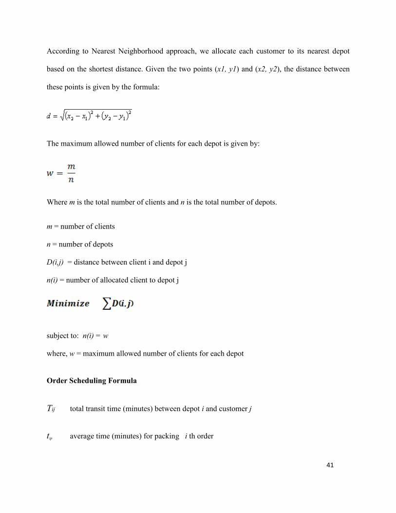
4.1.1 Nearest Neighbor
In the Nearest Neighbor approach, we pick each depot one by one and allocate the nearest
customers to it maintaining the load balancing constraints. The distance between any two given
points (x1, y1) and (x2, y2) is calculated using the following formula:
The maximum allowed number of clients (or load) for each depot is given by

24
Where m is the total number of clients and n is the total number of depots.
4.1.2 Tabu Search
Tabu search is a meta-heuristic technique used to solve optimization problems by tracking and
guiding the search (Golver and Laguna, 1997). Tabu search begins by setting up a set of feasible
solutions then choosing certain solutions in the feasible neighbourhood subject to constraints of
tabu list for searching the objective solution, and finally generating the solution. Tabu search
enhances the performance of a local search method by using memory structures, once a potential
solution has been determined then it is marked as tabu so that the algorithm does not visit that
possibility repeatedly. TS focus on the problem of how to cut off large computation in the
solution space so as to avoid long computation times and make the search quicker. The tabu list
length is an important factor in TS for the reason that its length will affect the computation speed
or the efficiency of the searching process and therefore be decided by the condition of problem
or other factors that affect the TS process. Glover (1989)
Method Description
Generate Initial Solution
This step involves generating initial solution which include of opening all facilities, random
allocation of clients, and evaluation of objective function for that solution.
Initialize memory structures

25
This step involves initialization of all memory structures used during the run of the tabu search
algorithm. The memory structures involved are tabu list, short-term and long-term memories.
The difference between short term and long term memory is that the short-term memory is the
list of solutions recently considered. If a potential solution appears on this list, it cannot be
revisited until it reaches an expiration point whereas the long-term memory is the rules that
promote diversity in the search process (Glover and Laguna, 1997).
Generate admissible solutions
Generate a set of candidate moves from the current solution which is the result of finding nearest
neighbourhood for each depots. A move describes the process of generating a feasible solution to
the problem. For example, Add, Drop, Swap etc. In our case, all these three kind of moves are
involved in allocating customers to logistics facilities or depots to generate a solutions
considering to satisfy balance allocation
Select best solution
This step returns the best solution from the list of candidate solution. If the best of these solutions
is not tabu or if the best is tabu but satisfies the aspiration criteria, the pick that move and
consider it to be the new current solution, else pick the best move that is not tabu and consider it
to be the new current solution. Repeat the procedure for a certain number of iterations. On
termination, the best solution obtained so far is the solution obtained by the algorithm.
The tabu status of solution approaches is maintained for number of iterations, the number of
previous solution being called the tabu tenure or tabu list length. Unfortunately, this may forbid
moves towards attractive, unvisited solutions. To avoid such an undesirable situation, an

26
aspiration criteria is used to override the tabu status of certain moves, it means if a certain move
is forbidden by tabu restriction, then the aspiration criteria, when satisfied, can make this move
allowable.
Update memory structures
To increase the efficiency of TS, long-term memory strategies can be used to intensify or
diversify the search. Intensification strategies are intended to explore more carefully promising
regions of the search space either by recovering elite solutions (i.e., the best solutions obtained so
far) or attributes of these solutions. Diversification refers to the exploration of new search space
regions through the introduction of new attribute combinations (Glover and Laguna 1997,
Dorigo and Stutzle, 2004).
Parameter setting
Following parameters need to be set before running the TS:
The number of random solutions to be generated from the current one.
The tabu list size.
Maximum number of non-improving iterations before termination.
Neighbourhood: A neighbourhood for this problem is defined as any other solution that is
obtained by an exchange of any two clients in the solution where a balance allocation is
considered. This always guarantees that any neighbourhood to a feasible solution is always a
feasible solution. If we considering the distance between each client and depot at each iteration
the neighbourhood with the best objective value (minimum distance) is selected.

27
The advantage of Tabu search is that it searches for good quality solutions over all the solution
space. It examines the trajectory or sequence of solutions and picks the best in the
neighbourhood iteration-wise, thereby, saving a lot of time in the process of computation
(Joubert, 2007). However, the disadvantage of Tabu Search is that it repeatedly searches for
solutions in its list, and therefore wastes a lot of time. Unfortunately, cutting off the runs due to a
time-limit will result in non-feasible solutions.
4.1.3 Greedy Heuristic
In the Greedy Heuristic, we pick any one depot at random and perform customer allocation using
the nearest distance criteria. The allocation continues till the depot reaches its maximum load.
Then, another depot is picked at random and the same process is repeated. We continue this
procedure until all the depots are reached or no more customers are available for allocation. The
principal advantage of greedy algorithm is that it is cheap, both in space and time. Because the
found solution may be local rather than global, the solution sometimes is not the desired one and
we will have to search for it again with different measures.
Figure 4.2 presents an illustration of results obtained from the implementation of the Greedy
algorithm for 3 depots and 15 customers. It can be seen that we do not obtain balanced allocation
with Greedy heuristic and therefore, alternate solution approaches are required.
4.1.4 Traditional Allocation
The traditional allocation is the process commonly used in practice by the logistics operators. It
involves allocating customers to logistics depots based on shortest distance. Sometimes, logistics
operators may also perform allocations based on the convenience of delivery and/or availability
of vehicles for delivery in those locations. In certain cases, logistics operators outsource services

28
for their far located clients, and therefore, in those cases, the clients will be served by third
parties and customer allocations be performed differently.
Figure 4.2: Greedy algorithm allocation result
4.1.5 Ant Colony Optimization
Ant Colony Optimization is a meta-heuristic technique based on the way ants search their foods,
that is, finding the shortest route by cooperation. It is a probabilistic technique for solving
complex computational problems by finding good paths through neighbourhoods. The various
steps of Ant Colony Optimization are as follows:
Initialization of ACO parameters and pheromone trials
Solution (Tour) Construction
Update of pheromone trials
The last two steps are carried out iteratively until no more improvement in objective function
value for customer allocations can be observed.

29
4.1.6 Combination of Nearest neighbor and Tabu search algorithm
This approach takes into account the advantages of Nearest neighbor and Tabu search algorithms
to generate good quality solutions. For the customer allocation problem, the Tabu search starts
off with a valid random allocation, and then moves the clients to nearest logistics depots
considering their capacity constraints. The algorithm terminates when no more improvement in
solution quality is observed or the maximum computation time has been reached. The initial
solution used in Tabu Search is generated using Nearest neighbor approach. Figure 4.3 presents
the result of this hybrid approach.
Figure 4.3: Our study allocation result

30
NN and Tabu Search Pseudo-Code
NN
Begin
For all clients
Find nearest neighborhood depots
End loop
TS
Begin
Initialize the tabu list
Initialize short-term
Setup initial solution using NN
Calculate the objective function for each depot
Generate Neighborhood
While (number if iterations <= Maximum value) or (improvement in objective function
value <= 10-3
) do
Begin
Move
Update Tabu list
Update Short-Term Memory
Check Aspiration Criteria
Pick the best move s” that is non-tabu or aspiration criteria
Setup new Neighborhood
End
End

31
To compare the performance of our model results, we compared it with other heuristics
mentioned above. Figure 4.4 presents the results of the different approaches. It can be seen that
our proposed approach integrating Tabu search and nearest neighbourhood algorithms gives the
best results in terms of uniform allocation of clients to the three depots and least distribution
costs to customers.

32
Figure 4.4: Result of different customer allocation

33
4.2 Order Scheduling
Order Scheduling involves generating a sequence or priority list for delivery of goods to
customers. The goal is to achieve high quality service with least distribution costs. To perform
order scheduling of customers residing in urban areas, the specificities of the city such as
congestion, incidents etc. cannot be neglected. Besides, the packing time, loading time,
unloading time, access times to city etc. are also important parameters that affect the order
scheduling process. Therefore, considering the importance of these critical factors for performing
order scheduling for urban areas, we propose a weighted scoring model for generating customer
priorities. The weighted service time for each customer = w1*Loading Time + w2*Transit time+
w3*Historical Delay Time(of city) + w4*Packing Time + w5*Access Time to Facility where
w1, w2, w3, w4 and w5 are the weights of criteria Loading Time, Transit time, Historical Delay
Time(of city), Packing Time and Access Time to Facility. Each of these times (or criteria) has
different weight which depends on the priorities of the logistics operator.
4.2.1 Genetic Algorithm
In order to solve to our scheduling plan by Genetic Algorithm, two main requirements are to be
satisfied: First a string can represent a solution of the solution space, and second an objective
function and hence a fitness function which measures the goodness of a solution can be defined.
We generate an initial population by using output of allocation section and each individual in the
population is called a chromosome, then take this initial population and cross it, combining
genomes along with a small amount of randomness (mutation).

34
We take this initial population and cross it, combining genomes along with a small amount of
randomness (mutation).
Fitness function
Since, scheduling for this problem is a minimization in terms of minimizing the total travel time
for delivering the orders, we consider below fitness function, where f(x) calculates total travel
time or weighted client score value as an objective function of the schedule.
Parents Selection Procedure
To select the parents for crossover, we have chosen the ranking method which is picking the best
individuals based on objective function value every time,
Crossover Operator
We select Pi for cross-over since it has the least objective function value; we also used the one-
point cross-over in our approach which involves randomly generating one cross-over point and
then swapping clients of the parent chromosomes in order to generate offspring.
Then we calculate the objective function for both offspring’s to can equal a new generation.
The offspring of this combination is selected based on an improving objective function, and new
offspring’s is returned back to the original population and replace with it.

35
We let this process continue until number of iterations <= 10000 or improvement in objective
function value <= 10^-3
Mutation Operator
Mutation is applied to each child after crossover. The mutation operator works by selecting
randomly one of the clients in the child chromosome and allocating to another place which
picked at random and while a crossover fraction considered 0 for this problem then all children
are mutation children.
Replacement population method
The newly generated child solutions are put back into the original population to replace the less
fit members. The average fitness of the population increases as child solutions with better
finesses replace the less fit solutions, so it means we used incremental replacement for this
problem.
Population size
The performance of GA is influenced by the population size. Small populations run the risk of
seriously under-covering the solution space, while large populations are computationally
intensive [Jaramillo et al, 2002]. we chose a population size equal to n which is equal to the
number of clients multiple related depots for this problem.
Population size = Number of clients * 2

36
The weighted service times for customers are input to the Genetic Algorithms for generating
schedules for order delivery to customers. We perform order scheduling for each cluster, which
is the results of first step of our study. Genetic algorithms (GA) are ideal for these types of
problems where the search space is large and the number of feasible solutions is small. The
various steps of GA are presented as follows:
Set up an initial set of random solutions called population. Each individual in the
population is called a chromosome.
Encode the solution into chromosomes.
Make crossover; then make mutation.
Get the offspring, or next generation from above step.
Decode and evaluate the parent and offspring generation.
Select current generation and form newer generation.
Repeat step 2 to step 6 till you get the satisfied solution while meeting the conditions.
We let this process continue either for a pre-allotted time or until we find a solution that fits our
objective function. It is also possible, of course, to add further fitness values such as minimizing
costs; however, each constraint that we add greatly increases the search space and lowers the
number of solutions that are good matches.

37
Genetic Algorithm Pseudo-Code
Begin
For all Depots
Begin
Choose initial population (random)
While (not terminate condition) do
Begin
Calculate the objective function for each chromosome
Calculate Fitness function = 1 / (total objective function)
Select chromosomes (Parents) with best fitness values
Perform crossover to Generate Offspring
If offspring same as parent chromosome
Apply mutation operator
Perform incremental replacement of population by replacing worst parent
with generated Offspring
End
End
End Loop
Genetic algorithm is an evolutionary search technique based on the Darwin’s principle “Survival
of the fittest”. The advantage of genetic algorithms is their ability to deal with problems without

38
regarding the inner characteristics, that is, they can handle any kind of objective functions, which
makes genetic algorithms very effective at performing global searches.
The limitations include slow speed and requirement of large memory space. Therefore, for
developing Genetic algorithms, we need to choose a computer with good CPU and speed.
4.3 Vehicle Allocation and Route planning for goods delivery
In this step, we perform vehicle allocation and route planning for goods delivery to customers.
The vehicle allocation is based on their capacity to meet order quantities, cost of allocation,
emission levels and noise. Using these criteria, we develop a weighted scoring model for vehicle
selection. The weighted score for each vehicle allocation solution = w1*cost + w2*emission +
w3*noise where w1, w2 and w3 are weights of criteria cost, emission, and noise respectively.
The vehicle allocation solution with lowest weighted score is finally selected.
The route planning involves calculation of fastest paths for goods delivery to customers. It takes
the allocation and scheduling plan as well as critical routing parameters such as shortest path and
vehicle capacities as input. We propose a modified Dijkstra’s algorithm for generating fastest
paths. The details of original and modified Dijkstra’s algorithm are presented as follows.
4.3.1 Dijkstra’s Algorithm
Dijkstra’s algorithm (1959) is a graph search algorithm that solves the single-source shortest path
problem for a graph with nonnegative edge path costs, producing a shortest path tree. Dijkstra’s
algorithm is often used in routing and as a subroutine in other graph algorithms (Cormen at al.
2001).
39
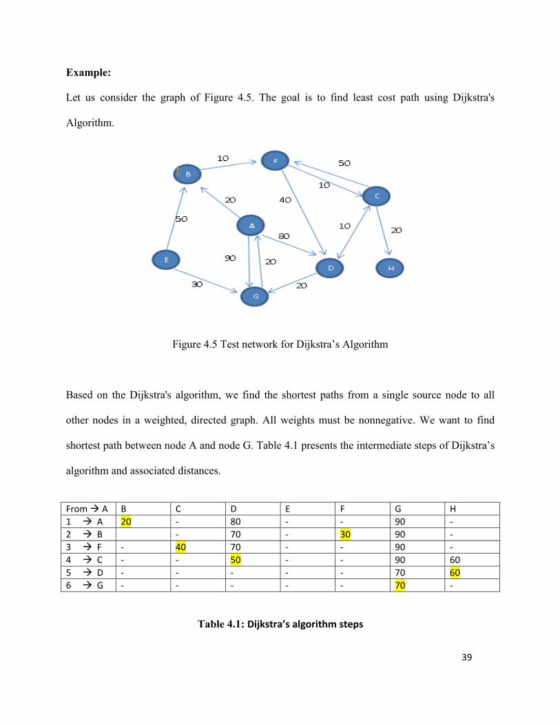
Example:
Let us consider the graph of Figure 4.5. The goal is to find least cost path using Dijkstra's
Algorithm.
Figure 4.5 Test network for Dijkstra’s Algorithm
Based on the Dijkstra's algorithm, we find the shortest paths from a single source node to all
other nodes in a weighted, directed graph. All weights must be nonnegative. We want to find
shortest path between node A and node G. Table 4.1 presents the intermediate steps of Dijkstra’s
algorithm and associated distances.
From A B C D E F G H
1 A 20 - 80 - - 90 -
2 B - 70 - 30 90 -
3 F - 40 70 - - 90 -
4 C - - 50 - - 90 60
5 D - - - - - 70 60
6 G - - - - - 70 -
Table 4.1: Dijkstra’s algorithm steps

40
So the resulting route is: A B F C D G assuming A is the origin and G is the
destination. The path length is 70.
4.3.2 Modified Dijkstra’s Algorithm
The Dijkstra's algorithm finds the shortest path between any given origin-destination pair. In order to
adapt it with respect to city traffic conditions, congestion, and access-timing regulations imposed by
municipal administrations for our problem, we will modify it and calculate fastest paths instead of
shortest distance. The fastest path will be calculated using the weighted distance = w1*Travel distance +
w2*Congestion Delay time + w3*Access Delay time where w1, w2 and w3 represent the weights of
criteria Travel Distance, Congestion Delay and Access Delay respectively.
Mathematical Modeling Approach
A goods distribution planning system can be formulated as a mathematical programming
problem, defined by an objective function, and a set of constraints to describe the structure of the
problem in mathematical ways. The objective function of this kind of problem is a non-linear
function, where it is difficult to achieve the optimal solution by mathematical approach, but for
this study we are trying to minimize the total goods distribution distance of overall trucks which
is as follows:
Client Allocation Formula
41
According to Nearest Neighborhood approach, we allocate each customer to its nearest depot
based on the shortest distance. Given the two points (x1, y1) and (x2, y2), the distance between
these points is given by the formula:
The maximum allowed number of clients for each depot is given by:
Where m is the total number of clients and n is the total number of depots.
m = number of clients
n = number of depots
D(i,j) = distance between client i and depot j
n(i) = number of allocated client to depot j
subject to: n(i) = w
where, w = maximum allowed number of clients for each depot
Order Scheduling Formula
Tij total transit time (minutes) between depot i and customer j
tip average time (minutes) for packing i th order

42
til average loading time (minutes) for i th order
tit average access time (minutes) to transportation facilities for depot i
xti parameter for the availability of depot i at time t
Total transit time is the sum of the average delivery time between the customer and the depots
(tij), transportation facility access time (tik), and the average access time between depot and the
supplier (til).
So, the objective function for the order scheduling formula is written as:
tiitilipij
xtttTMinimize
Routing Formula
Notations:
i = Job that is assigned to truck; i ∈ {1,2,3,…, n}
l = Position that job occupied in a tour; l ∈ {1,2,3,…, m}
k = Truck number; k ∈ {1,2,…, m}
m = Number of truck;
oi = Order from customer i
n = Actual number of locations; n∈{23}
r = Upper bound of number of locations visited daily
di, j
= Distance between node i to node j

43
wi = Weight of order for i (in kgs)
W = Truck capacity
Then,
Total number of jobs (dummy and non-dummy) = Tn
The decision variables:
x i, k
= 1; if node i assigned to truck k
x i, k
= 0; otherwise
yi, l, k
= 1; if node i occupies position l in the tour for truck k
= 0; otherwise
This formula is subject to the load of all trucks which should not exceed its capacity
We can assign the job i to one and only one truck at a time
For each job i which is assigned to truck k it takes one position 1 in the tour that truck k
performs
Every job i takes only one position in the tour which is performed by truck k

44
Job i takes one position in the tour which is performed by truck k if job i is assigned to
truck k

45
Chapter 5:
Numerical Study
5.1 Six-Customer, 2-Depot Problem
Let us consider a distribution network containing 2 logistical facilities (depots) and 6 customers.
The information on minimum travel time (MTT), access regulation delay (ARD), time regulation
delay (TRD), and congestion delay (CD) between the various customers and the depots is
provided in Table 5.1. The weights of the criteria shown in Table 5.1 are presented in Table 5.2.
Table 5.1: Allocation criteria values for the 6 customer problem
D1
Criteria C1 C2 C3 C4 C5 C6
MTT 13.4 15.3 7.5 6.7 16.4
5.7
ARD 4.9 4.5 2.5 3.1
5.1 2.9
TRD 10.9 11 3.7 3.5 12.2 3.4
CD 9.8 10.4
4.8
4.3 8.7 4.3
Weighted Travel Time 12.2 14.1 5 4.2 15.7 3.6
D2
Dist 9.3 8.7 8.7 16.3 6.4
14.7
MTT 4.8 4.5 4.7 4.5 2.1 5.8
TRD 5.9 4.3 3.7 11 2.2 11.8
CD 8.6 10.4
11.8
12.4
3.4 9.8
Weighted Travel Time 9.2 9.8 9.9 15.3 5.7 11.4

46
Table 5.2: Allocation criteria with weights
The weighted travel time for the six customers computed using the information presented in
Tables 5.1-5.2 is presented in Table 5.3.
Table 5.3: Weighted Travel Time for 6-customer problem
5.1.1 Customer Allocation
We generate the primary solutions based on finding nearest neighbourhood for each depot and
also we considering the balance allocation then we select the solution which returns lowest value
as a initial solution
Criteria Weight
Minimum Travel Time 60%
Access regulation delay
5%
Time regulation delay 5%
Congestion delay 30%
Weighted Travel Time 100%
D1 D2 C1 C2 C3 C4 C5 C6
D1 0
D2 14.9 0
C1 9.2 12.2 0
C2 14.1 9.8 2 0
C3 5 9.9 9.2 11.2 0
C4 7.2 15.3 15 17 6.1 0
C5 15.7 14.7 5.4 5 11.4 17.4 0
C6 3.6 11.4 9 11 2 6.1 12.1 0

47
D1: C1C6C4 (Weighted Travel Time = 20)
D2: C3C5C2 (Weighted Travel Time = 34.4)
Overall objective function value so far for initial solution is
D1C1C6C4D1D2C3C5C2D2=20+34.4 = 54.4. The initial solution is now input into the Tabu
Search for further improving the solution quality. Let us generate a neighbourhood solution
Neighbourhood: A neighbourhood for this problem is defined as any other solution that is
obtained by an exchange of any two clients in the solution where a balance allocation is
considered. This always guarantees that any neighbourhood to a feasible solution is always a
feasible solution. If we considering the distance between each client and depot, at each iteration
the neighbourhood with the best objective value (minimum distance) is selected.
Generating
neighbour
D1C1C6C4D1 D1C1C3C4D1
D2C2C3C5D2 D2C2C6C5D2
New Neighbourhood = {(D1, C1,C3,C4), (D2, C2,C6,C5)}
D1C1C3C4D1D2C2C6C5D2 =57.3
The new neighbourhood solutions are generated as follows:
D1C1C3C4D1D2C2C6C5D2 =57.3 (S1)
D1C1C5C4D1D2C3C2C6D2=63.2 (S2)
D1C1C5C6D1D2C2C3C4D2=63.5 (S3)
D1C2C5C6D1D2C1C4C3D2=70.8 (S4)
D1C3C4C6D1D2C1C5C2D2=52.5 (S5)
D1C4C3C2D1D2 C1C5C6 D2=64.6 (S6)

48
After a move that exchanges the positions of element C6 and C3 in a sequence for S1 solution, ,
we would like to prevent elements C6 and C3 from exchanging positions in the next Tabu
Tenure iterations
Tabu activation rule: move (Ci Cj) is tabu if both Ci and Cj are tabu-active
The C6-C3 in solution S1 is also can added to the tabu list for avoid repetitive solutions if the
new solution is better than the previous one and is not present in the tabu list and we continue
this method for all solutions.
Tabu list
Tabu list with elements (D1C3-D2C6, D3C9-D4C12, D5C15-D6C18)
Consequently we are able to generate different neighbourhood from current solution through
dropping and adding clients to current solution, we generate solutions in the neighbourhood of
S5 and repeat the whole process again for updating best solution at every iteration.
In the neighbourhood, the best feasible solution emerges to be (S5) with the least objective
function (travel time) value = 52.5 The difference between the initial and the current solution
(S5) is given by 2.1 (value has actually reduced):
Can-now= D1C3C4C6D1D2 C1C5C2 D2=5+7.2+3.6+12.2+14.7+9.8=52.5
Δf= D1C1C6C4D1D2C3C5C2D2- D1C3C4C6D1D2 C1C5C2 D2=54.4-52.5=2.1
We exchange customers C4 and C5 in (S5) and the new allocation (S6) is given by.
D1C3C5C1D1D2 C6C4C2 D2=5+15.7+9.2+11.4+15.3+9.8=66.4 (S6)

49
Δf= D1C3C5C1D1D2C6C4C2D2- D1C3C4C6D1D2C1C5C2D2=66.4-52.5=13.9
It can be seen that the objective function value has increased. Therefore, (S6) will be added to
the tabu list by replacing the second worst objective function solution (S1). Now, we exchange
customers C6 and C2 in (S6) to generate the new solution.
D1C3C4C2D1D2C5C1C6D2=5+7.2+14.1+14.7+12.2+11.4=64.6 (S7)
Δf= D1C3C4C2D1D2C5C1C6D2- D1C3C4C6D1D2 C1C5C2 D2=64.6-52.5=12.1
Now we exchange between C3 and C5:
D1C1C2C5D1D2C4C3C6D2=9.2+14.1+15.7+15.3+9.9+11.4=75.6 (S8)
Δf= D1C1C2C5D1D2C4C3C6D2- D1C3C4C6D1D2 C1C5C2 D2=75.6-52.5=23.1
As, (S8) has the worst objective function value, it will not be put in the tabu list. Now, we use the
3 elements change method, and generate feasible solutions (neighbourhood) by putting C1C2C5
after C6:
D1C4C3C6 D 1D2C1C2C5D2=5+7.2+3.6+12.2+9.8+14.7=52.5 (S9)
Δf= D1 C 4C3C6 D 1D2C1C2C5D2- D1C3C4C6D1D2 C1C5C2 D2=52.5-52.5=0 (N)
Since, M has the least objective function value so far, we renew tabu list (I,E,C,B, H).
We continue computations in this way and find that the newer values of objective function, we
could use (S9) as the best solution. In fact, it is the best actual solution from beginning.
Short-Term Memory: we considering the short-term memory for this problem and it is the list
of recent solutions. If a potential solution appears on this list, it cannot be revisited until it
reaches an expiration point, and expiration point for this problem is termination of algorithm.
50
STM List = (S0,S1,S2,S3,..,S9)
Aspiration Criteria: We define the aspiration criteria as a solution involving tabu move that
has better objective value than best known answer, then the tabu status is disregarded.
An aspiration criteria is used to overrule the tabu restriction, therefore we can consider the
attractive unvisited solution as well
Diversification: some times, the process may get trapped in a space of local optimum. To allow
the process to search other parts of the solution space, it is required to diversify the search
process, driving it into new regions. This is implemented in the this problem with swaps a client
with different depots which means we can swaps C6 from Depots 1 to C3 from Depots 2.
C6D1 C3D2
Termination criteria: The algorithm terminates if it meets any one of the following criteria:
a. It reaches a 8,000 iterations.
b. The objective function is improved with 15% improvement to compare with initial solution.
c. There is no improvement in the solution for last 8,000 iterations.
This process continues until maximum number of iterations have been reached or very minimal
improvement in objective function value (say <= 10-5
) is observed.
The results of customer allocation obtained using the Nearest Neighbor and Tabu Search
approach are presented in following.

51
D1 C4C3C6
D2 C1C2C5
5.1.2 Scheduling
The order scheduling of customers in the clusters obtained from previous step is performed using
Genetic algorithm. Table 5.4 presents the order details of the customers.
Client Depot Order
C1 D2 4000
C5 D2 1000
C3 D1 2500
C4 D1 200
C2 D2 2000
C6 D1 1500
Table 5.4: Order Quantity for six customer problem
Table 5.5 presents the information required for scheduling of customers C1 to C6. We are
assuming that these orders have been requested during a common time window. In case, the
customers have different time windows then we will first group the customers based on their
preferred time windows and then schedule each group in a similar way. The objective is to
minimize the total service time and distribution costs (weighted score of different criteria as
indicated in last row Table 5.5) for all clients.
Criteria Weight C1-D2 C2-D2 C3-D1 C4-D1 C5-D2 C6-D1
Loading Time 10% 50
50
50 50 50 50
Transit time 30% 70 90 50 75 80 60
Historical Delay Time(city) 20% 60 70 80 50 60 40
Packing Time 15% 50 60 40 50 40 30
Access Time to Facility 10% 0 10 10 90 0 10
Unloading Time 15%
90 50 60 20 10 70
Weighted Service Time (Min) 100% 58 64 52.5 57 48.5 47
Table 5.5: Order scheduling information for six customer problem

52
The weighted Service Time presented in last row of Table 5.5 is calculated using the weighted
scoring model for customers C1-C6 as follows:
C1= (10*50)+(30*70)+(20*60)+(15*50)+(10*0)+(15*90) = 5800
C2= (10*50)+(30*90)+(20*70)+(15*60)+(10*10)+(15*50) = 6400
C3= (10*50)+(30*50)+(20*80)+(15*40)+(10*10)+(15*60) = 5250
C4= (10*50)+(30*75)+(20*50)+(15*50)+(10*90)+(15*20) = 5700
C5= (10*50)+(30*80)+(20*60)+(15*40)+(10*0)+(15*10) = 4850
C6= (10*50)+(30*60)+(20*40)+(15*30)+(10*10)+(15*70) = 4700
From step 1, we know that the following customers are allocated to depot 1 and 2.
D1 C4C3C6
D2 C1C2C5
We will use Genetic Algorithm to schedule the customer orders. Initially, we will generate a set
of solutions for depot D1:
Function:
S1= D1C4C3C6D1
S2= D1C6C4C3D1
S3= D1C4C6C3D1
S4= D1C3C4C6D1
S5= D1C3C6C4D1
S6= D1C6C3C4D1
FS1= D1C4C3C6D1 =193.5
FS2= D1C6C4C3D1 =205.5
FS3= D1C4C6C3D1 =198.5
FS4= D1C3C4C6D1 =205.5
FS5= D1C3C6C4D1 =198.5
FS6= D1C6C3C4D1 =193.5
The initial population for depots 1 consists of six chromosomes P1, P2 ,P3 ,P4,P5,P6 generated
at random.

53
Solution String Objective Function
P1 1 4 3 6 1 193.5
P2 1 6 4 3 1 205.5
P3 1 4 6 3 1 198.5
P4 1 3 4 6 1 205.5
P5 1 3 6 4 1 198.5
P6 1 6 3 4 1 193.5
We take this initial population and cross it, combining genomes along with a small amount of
randomness (mutation).
Fitness function
Since, scheduling for this problem is minimizing the total travel time for delivering the orders,
we consider below fitness function, where f(x) calculates total weighted service time as an
objective function of the schedule.
Parents Selection Procedure
To select the parents for crossover, we have chosen the ranking method which is picking the best
individuals based on objective function value every time,
P1< P2 & P1< P3 & P1< P4 & P1< P5 then P1 is selected.
Crossover Operator

54
We select P1 for cross-over since it has the least objective function value; we also used the one-
point cross-over in our approach which involves randomly generating one cross-over point and
then swapping clients of the parent chromosomes in order to generate offspring.
O1 D1 C3 C4 C6 D1
And
O2 D1 C6 C3 C4 D1
We calculate the objective function for both offspring’s to can equal a new generation.
FO1= D1C3C4C6D1=205.5
FO2=D1C6C3C4D1=193.5
The offspring of this combination is selected based on an improving objective function, so the
offspring FO2 is the same as parent chromosomes therefore, the new offsprings O2 can be
returned back to the original population and replace with P1.
So for Iteration number two we have:
S1= D1C6C3C4D1
S2= D1C6C4C3D1
S3= D1C4C6C3D1
S4= D1C3C4C6D1
S5= D1C3C6C4D1
S6= D1C6C3C4D1
We let this process continue for each depots until number of iterations <= 5000 or improvement
in objective function value <= 10^-3

55
Mutation Operator
Mutation is applied to each child after crossover. The mutation operator works by selecting
randomly one of the clients in the child chromosome and allocating to another place which
picked at random and while a crossover fraction considered 0 for this problem then all children
are mutation children.
O1 C4 C3
O2 C4 C6
Replacement population method
The newly generated child solutions are put back into the original population to replace the less
fit members. The average fitness of the population increases as child solutions with better
finesses replace the less fit solutions, so it means we used incremental replacement for this
problem.
Population size
The performance of GA is influenced by the population size. Small populations run the risk of
seriously under-covering the solution space, while large populations are computationally
intensive [Jaramillo et al, 2002]. we chose a population size equal to n which is equal to the
number of clients multiple related depots for this problem.
Population size = Number of clients * 2 (begin and end depot) = 6

56
Therefore, the final order schedule for depot 1 using the proposed GA approach is C6C3C4 and
for depot 2 is C2C5C1.
5.1.3 Vehicle allocation and Routing
Table 5.6 presents the different vehicle types, their capacities, emission factors and noise.
No Type Quantity
(truck)
Capacity
(ton)
Operating
Cost
(Dollars
per day)
Emission
Factor
Noise
1 Small Size Truck
(S)
6 1 350 Low (15) Low (10)
2 Big Size Truck
(B)
3 5.5 600 High (60) High (35)
3 Medium Truck
(M)
4 3 500 Medium(35) Medium (20)
Table 5.6: Vehicle Details for six customer problem
For depots 1 and 2, we have the following scheduled orders:
Depot 1 = C6C2C3 (Order quantity = 6000) and Depot 2 = C4C5C1 (Order quantity = 5200)
To serve order quantities for customers of depots 1 and 2, two solutions for vehicle allocations
are possible.
Solution 1: Using 2 medium size truck (Capacity = 3000+3000 = 6000)
Solution 2: Using 1 big and 1 small truck (Capacity = 5500+1000 = 6500)
Now, we will evaluate these two solutions using weighted scoring method. Table 5.7 presents the
evaluation results using the cost, emissions and noise criteria.

57
Table 5.7: Solution weight scoring for 6 customer problem
Since, the weighted score of solution 2 is less than solution 1, so we choose solution number 2
for vehicle allocation.
Now, we will generate shortest path for the vehicles (solution 2) using Modified Dijkstra’s
algorithm to serve the clients of depot 1. Table 5.8 represents the weighted distance used in
modified Dijkstra’s algorithm for planning shortest paths for customers of depot 1.
Table 5.8: Distance data for depot 1 (or group A)
Figure 5.1 presents the test network for depot 1 (or group A). Using modified Dijkstra’s
algorithm, the fastest path for depot 1 (group A) is: A C6 C3 C4 A . Likewise, the
Weight
Solution 1 (2M)
Solution2 (1 B,1 S)
Cost 70% 1000 950
Emission 20% 70 75
Noise 10% 40 45
Weight 100% 718 684.5
D1
C6
C3
C4
D1 0 3.6 14 5
C6 3.6 0 11 2
C3 14 11 0 11.2
C4 5 2 11.2 0

58
fastest path for depot 2 (group B) is calculated. The solution is given by B C2 C5 C1
B.
Figure 5.1: Test Network for group A
The allocation, scheduling and routing results for the 6-customer problem are summarized In
Table 5.9. It can be seen that the objective function has improved (or weighted travel time
reduced) for the allocation and scheduling problems. For the routing problem, the objective
function remains unchanged.
Problem
Type
Initial solution
Distance Total
Distance
Final Solution
(TS)
Distance Total
Distance
Allocation
(NN-TS
Approach)
D1 C1C6C4 20 54.4 D1 C4C3C6 22.7 52.9
D2 C3C5C2 34.4 D2 C1C2C5 30.2
Scheduling
(GA
Approach)
D1 C4C3C6
D1
30.9 78.2 S1
D1C6C3C4D1
30.8 78.1
D2 C1C2C5
D2
47.3 S1
D2C2C5C1D2
47.3
Routing
(Modified
Dijkstra’s)
S1
D1C6C3C4D1
30.8 78.1 R1 D1 C6
C3 C4
D1
30.8 78.1
S1
D2C2C5C1D2
47.3 R1 D2 C2
C5 C1
D2
47.3
Table 5.9: Solution summary for 6-customer problem

59
5.2 Model Verification
To verify the model results, we tested our model under three different problem instances. The
first problem is same as present in section 5.1. The second problem involves 21 customers and 7
depots. The third problem involves 50 customers and 5 depots. We performed Client allocation,
Order Scheduling and Vehicle Routing for these problems using the TS-NN, GA, Weighted
Scoring and Modified Dijkstra’s algorithm.
5.2.1. Twenty One - Customers, Seven - Depots problem
Table 5.10 presents the weighted travel times, customer demands and the capacities of the seven
depots. The weights of the criteria Minimum travel time, Access Regulation Delay, Time
Regulation Delay are same as in Table 5.2.
Depots demand
D1 D2 D3 D4 D5 D6 D7
C1 3.4 3.74 4.2 3.2 3.3 4.8 2.1 120
C2 3.10 3.28 3.3 2.7 4.0 3.1 5.8 200
C3 3. 8 3. 4 3.2 2.9 3.0 2.4 4.8 80
C4 3.5 3.6 3.5 4.9 3.6 2.5 4.9 110
C5 3.7 3.0 3.2 4.6 2.0 3.2 4.6 130
C6 3.6 3.7 3.6 4.7 3.7 3.8 4.7 90
C7 2.88 2.97 7.3 3.31 3.5 3.6 4.5 140
C8 2.5 2.9 3.0 2.83 2.7 3.0 3.2 170
C9 2.6 2.7 4.82 3.2 3.6 3.7 10.8 90
C10 5.8 2.8 3.2 5.3 4.74 4.2 6.1 115
C11 3.1 2.9 6.7 3.0 3.28 3.3 4.4 100
C12 2.4 2. 7 2.9 5.0 3.24 6.5 2.0 125
C13 3.5 3.30 3.5 3.6 9.04 2.8 4.5 85

60
Table 5.10 Weighted travel times, capacity and demand data for 21 customer problem
For this sample we consider 7 logistics depots D1,D2,D3,D4,D5,D6,D7 and 21 customers C1,
C2, …, C21 respectively. We generate the primary solutions based on finding nearest
neighborhood for each depot and also we considering the balance allocation.
S(A)=(D1,C1,C2,C3,D2,C4,C5,C6,D3,C7,C8,C9,D4,C10,C11,C12,D5,C13,C14,C15,D6,C16,C
17,C18,D7,C19,C20,C21) = 84.91
S(B)=(D1,C1,C2,C3,D2,C7,C8,C18,D3,C19,C20,C21,D4,C4,C5,C6,D5,C13,C14,C12,D6,C16,C
17,C18,D7,C9,C10,C11) = 92.68
S(C)=(D1,C3,C15,C14,D2,C16,C18,C19,D3,C8,C20,C21,D4,C4,C5,C6,D5,C13,C2,C7,D6,C1,C
17,C12,D7,C9,C10,C11) = 98.54
S(D)=(D1,C3,C10,C18,D2,C4,C17,C21,D3,C7,C20,C11,D4,C12,C5,C2,D5,C13,C2,C19,D6,C1,
C8,C16,D7,C9,C14,C15) = 102.07
Then we check the feasibility for this generated solution and then we select the solution which
returns lowest value as a initial solution .
C14 4.2 2.96 2.7 1.0 3.03 3.0 2.3 180
C15 3.1 3.2 2.6 2.74 2.82 3.7 4.1 130
C16 3.2 4.3 2.8 2.88 3.2 3.3 2.8 95
C17 2.7 5.0 3.1 2.92 5.7 6.0 3.1 175
C18 5.9 3.0 2.4 2.47 2.9 3.0 2.4 150
C19 3.5 1.6 3.5 1.30 3.5 3.6 7.5 190
C20 2.7 3.0 5.2 2.96 2.7 3.0 1.2 95
C21 2.6 3.7 4.8 3.28 3.6 6.7 3.8 160
Capacity 800 800 1100 1000 700 1100 900

61
S0 = {(D1, C1,C2,C3),(D2, C4,C5,C6) ,(D3, C7,C8,C9),(D4, C10,C11,C12) ),(D5,
C13,C14,C15) ,(D6, C16,C17,C18) ,(D7, C19,C20,C21))}
D1C1C2C3D1D2C4C5C6D2D3C7C8C9D3D4C10C11C12D4D5C13C14C15D5D6C16C17C18
D6D7C19C20C21D7= 84.91
Overall objective function value so far for initial solution is = 84.91.
Let us generate a neighboring solution
Neighbourhood: A neighbourhood for this problem is defined as any other solution that is
obtained by an exchange of any two clients in the solution where a balance allocation is
considered. This always guarantees that any neighbourhood to a feasible solution is always a
feasible solution. If we considering the distance between each client and depot, at each iteration
the neighbourhood with the best objective value (minimum distance) is selected.
Generating neighbor
D1C1C2C3D1 D1C1C2C6D1
D2C4C5C6D2 D2C4C5C3D2
D3C7C8C9D3 D3C7C8C12
D4C10C11C12D4 D4C10C11C9
D5C13C14C15D5 D5C13C14C18
D6C16C17C18D6 D6C16C17C15
D7C19C20C21D7 D7C19C20C21

62
New Neighbourhood S1 = {(D1, C1,C2,C6), (D2, C4,C5,C3) ,(D3, C7,C8,C12),(D4,
C10,C11,C9) ,(D5, C13,C14,C18),(D6, C16,C17,C15) ,(D7, C19,C20,C21))} .
S1 = {(D1, C1,C2,C6), (D2, C4,C5,C3) ,(D3, C7,C8,C12),(D4, C10,C11,C9) ,(D5,
C13,C14,C18),(D6, C16,C17,C15) ,(D7, C19,C20,C21))} .
D1C1C2C6D1D2C4C5C3D2D3C7C8C12D3D4C10C11C9D4D5C13C14C18D5D6C16C17C15
D6D7C19C20C21D7 =81.87
After a move that exchanges the positions of element C3,C9,C15 and C6,C12,C18 in a sequence
for S1 solution, , we would like to prevent elements C3,C9,C15 and C6,C12,C18 from
exchanging positions in the next Tabu Tenure iterations
Tabu activation rule: move (Ci Cj) is tabu if both Ci and Cj are tabu-active
The C3-C6 , C9-C12, C15-C18 in solution S1 is also added to the tabu list for avoid repetitive
solutions from entering into the tabu list.
Since, the new solution is better than the previous one and is not present in the tabu list the new
solution is accepted and updated as the best solution.
{D1(C1,C2,C6),D2(C4,C5,C3),D3(C7,C8,C12),D4(C10,C11,C9),D5(C13,C14,C18),
D6(C16,C17,C15),D7(C19,C20,C21)}
Tabu list
Let us initiate the Tabu list with elements (D1C3-D2C6, D3C9-D4C12, D5C15-D6C18)

63
Consequently we are able to generate different neighborhood from current solution through
dropping and adding clients to current solution, we generate solutions in the neighborhood of S1
and repeat the whole process again for updating best solution at every iteration.
A tabu move will be considered only if, it would result in an improving objective function than
the initial solution found previously.
New Neighbourhood S2 = {(D1, C1,C2,C4), (D2, C6,C8,C3) ,(D3, C7,C5,C12),(D4,
C18,C11,C9) ,(D5, C13,C14,C10),(D6, C21,C17,C15) ,(D7, C19,C20,C16))} .
D1C1C2C4D1D2C6C8C3D2D3C7C5C12D3D4C18C1C9D4D5C13C14C10D5D6C21C17C15
D6D7C19C20C16D7 =83.38
Since, the solution S2 is not improved than the previous one so the new solution is not accepted .
To preventing cycling and re-visiting previously visited solution tabu move restrictions are
employed. In our implementation we classify a solution obtained by swapping the clients as a
tabu if it corresponds to the same swapping which was swapped in an accepted solution.
Short-Term Memory: we considering the short-term memory for this problem and it is the list
of recent solutions. If a potential solution appears on this list, it cannot be revisited until it
reaches an expiration point, and expiration point for this problem is termination of algorithm.
STM List = (S0,S1,S2)

64
Aspiration Criteria: We define the aspiration criteria as a solution involving tabu move that
has better objective value than best known answer, then the tabu status is disregarded.
An aspiration criteria is used to overrule the tabu restriction, therefore we can consider the
attractive unvisited solution as well
Diversification: some times, the process may get trapped in a space of local optimum. To allow
the process to search other parts of the solution space, it is required to diversify the search
process, driving it into new regions. This is implemented in the this problem with swaps a client
with different depots which means we can swaps C1 from Depots 1 to C20 from Depots 7.
C1D1 C20D7
Termination criteria: The algorithm terminates if it meets any one of the following criteria:
a. It reaches a 100,000 iterations.
b. The objective function is improved with 15% improvement to compare with initial solution.
c. There is no improvement in the solution for last 100,000 iterations.
This process continues until maximum number of iterations have been reached or very minimal
improvement in objective function value (say <= 10-5
) is observed.
The results of customer allocation obtained using the Nearest Neighbor and Tabu Search
approach are presented in Table 5.11. It can be seen that the objective function value has
improved with respect to the initial solution.

65
Depots Initial
solution
(NN)
Distance Total
Distance
Final Solution
(TS)
Distance Total
Distance
D1 C1,C2,C3 6.5 85 D1 C6C7C8 8.98 53.38
D2 C4,C5,C6 10.3 D2 10C11C9 8.4
D3 C7,C8,C9 15.12 D3 C15,C16,C17 8.5
D4 C10,C11,C12 13.3 D4 C2,C14,C19 5
D5 C13,C14,C15 14.98 D5 C20,C5,C21 8.3
D6 C16,C17,C18 12.3 D6 C13,C3,C4 7.7
D7 C19,C20,C21 12.5 D7 C1,C12,C18 6.5
Table 5.11: Allocation Results for the 21 customer problem
Table 5.12 presents the customer order information for the allocated clients.
Depot
Id
Client
Id
Order
Quantity
D1 C6 4200
D1 C7 4500
D1 C8 4500
Table 5.12: Order Data for 21-customer problem
Table 5.13 presents the other information used for scheduling orders of customer clusters
obtained from step 1.
Customers
Criteria
Loading Time
Transit time
Historical Delay
Time(city)
Packing Time
Access Time to Facility
Unloading Time
Weighted Client Score
10% 30% 20% 15% 10% 15% 100%
C1-D7 50 40 60 40 20 10 3850

66
C2-D4 50 45 30 60 80 30 4600
C3-D6 40 55 35 75 95 20 5125
C4-D6 50 25 40 80 60 35 4375
C5-D5 40 65 55 30 95 15 5075
C6-D1 60 52 38 86 32 18 4800
C7-D1 78 24 58 90 34 26 4740
C8-D1 45 36 72 80 95 15 5345
C9-D2 12 28 36 92 74 60 4700
C10-D2 56 88 25 40 80 75 6225
C11-D2 84 55 65 55 30 80 6115
C12-D7 12 48 52 38 86 30 4480
C13-D6 18 42 40 60 30 86 4730
C14-D4 94 25 40 24 35 90 4550
C15-D3 57 78 40 36 40 80 6321
C16-D3 16 45 40 28 55 92 4653
C17-D3 18 40 40 88 38 40 4872
C18-D7 30 45 45 55 60 55 3879
C19-D4 55 55 55 35 75 38 5423
C20-D5 47 25 25 40 80 60 4879
C21-D5 80 65 65 55 30 95 5210
Table 5.13: Order scheduling information for 21 customer problem
In order to solve to our scheduling plan by Genetic Algorithm, two main requirements are to be
satisfied: First a string can represent a solution of the solution space, and second an objective
function and hence a fitness function which measures the goodness of a solution can be defined.
We generate an initial population by using output of allocation section and each individual in the
population is called a chromosome, then take this initial population and cross it, combining
genomes along with a small amount of randomness (mutation).
S1= D1C6C7C8D1

67
S2= D1C7C6C8D1
S3= D1C8C6C7D1
S4= D1C6C8C7D1
S5= D1C7C8C6D1
S6= D1C8C7C6D1
We continue to set up the initial population for all different depots, and then we calculate the
objective function based on weight scoring result for each population.
FS1= D1C6C7C8D1=37.3
FS2= D1C7C6C8D1=25.32
FS3= D1C8C6C7D1=32.48
FS4= D1C6C8C7D1=25.32
FS5= D1C7C8C6D1=32.48
FS6= D1C8C7C6D1=37.3
The initial population for depots 1 consists of six chromosomes P1, P2 ,P3 ,P4,P5,P6 generated
at random.
Solution String Objective Function
P1 1 6 7 8 1 37.3
P2 1 7 6 8 1 25.32
P3 1 8 6 7 1 32.48
P4 1 6 8 7 1 37.3
P5 1 7 8 6 1 25.32
P6 1 8 7 6 1 32.48
We take this initial population and cross it, combining genomes along with a small amount of
randomness (mutation).

68
Fitness function
Since, scheduling for this problem is a minimization in terms of minimizing the total travel time
for delivering the orders, we consider below fitness function, where f(x) calculates total travel
time or weighted client score value as an objective function of the schedule.
Parents Selection Procedure
To select the parents for crossover, we have chosen the ranking method which is picking the best
individuals based on objective function value every time,
P2< P1 & P2< P3 & P2< P4 & P2< P5 & P2< P6 then P2 is selected.
Crossover Operator
We select P2 for cross-over since it has the least objective function value; we also used the one-
point cross-over in our approach which involves randomly generating one cross-over point and
then swapping clients of the parent chromosomes in order to generate offspring.
O1 D1 C7 C8 C6 D1
And
O2 D1 C8 C6 C7 D1
We calculate the objective function for both offspring’s to can equal a new generation.
FO1= D1C7C8D1C6=25.3

69
FO2=D1C7D1C6C8=32.48
The offspring of this combination is selected based on an improving objective function, so the
offspring FO1 is lower than the parent chromosomes therefore, the new offsprings O1 is returned
back to the original population and replace with P2.
We let this process continue until number of iterations <= 5000 or improvement in objective
function value <= 10^-3
Mutation Operator
Mutation is applied to each child after crossover. The mutation operator works by selecting
randomly one of the clients in the child chromosome and allocating to another place which
picked at random and while a crossover fraction considered 0 for this problem then all children
are mutation children.
O1 C8 C6
O2 C7 C8
Replacement population method
The newly generated child solutions are put back into the original population to replace the less
fit members. The average fitness of the population increases as child solutions with better
finesses replace the less fit solutions, so it means we used incremental replacement for this
problem.
Population size

70
The performance of GA is influenced by the population size. Small populations run the risk of
seriously under-covering the solution space, while large populations are computationally
intensive [Jaramillo et al, 2002]. we chose a population size equal to n which is equal to the
number of clients multiple related depots for this problem.
Population size = Number of clients * 2 = 6
The results of order scheduling using the proposed Genetic Algorithm approach are presented in
Table 5.14. It can be seen that the objective function value has improved with respect to the
initial solution.
Depots Initial
solution
(TS)
Distance Total
Distance
Final Solution
(GA)
Distance Total
Distance
D1 D1
C6C7C8
D1
27.3 121.84 S1 D1C7C6C8D1 16.32 91.88
D2 D2
10C11C9
D2
24.1 S1 D210C9C11D2 9.6
D3 D3
C15,C16,C17
D3
11.3 S1
D3C16C15C17D3
8.5
D4 D4
C2,C14,C19
D4
22.15 S1
D4C2C19C14D4
22.28
D5 D5
C20,C5,C21
D5
12.46 S1 D5C5C21C20
D5
12.26
D6 D6
C13,C3,C4
D6
12.83 S1
D6C3C13C4D6
11.9
D7 D7
C1,C12,C18
D7
11.7 S1 D7C18C1C12
D7
11.02
Table 5.14: Scheduling results for 21- Customer problem

71
To calculate the number of vehicles required to deliver the orders of depot 1, we will need the
order quantity requested by the clients. Using the Table 5.13 data, the total order quantity
requested by clients of depot 1 = 13200. Using the truck information presented in Table 5.6, we
find that two solutions are possible to meet this demand.
Solution 1 = 2 Big Truck + 1 Medium Truck =2 * 5500 = 11000 + 1* 3000 = 14000 >13200,
hence sufficient to meet the demand.
Solution 2 = 2Big Truck + 3 small truck = 2*5500+ 3*1000 = 14000 > 13200.
To make the final selection, we will compare the weighted scores for the two solutions as shown
in Table 5.15. Since the score of Solution 1 is lesser than Solution 2, therefore Solution 1 is
finally selected for vehicle allocation.
Table 5.15: Solution weight scoring for the 21 customer problem
To generate the vehicle routes, we will use the modified Dijkstra’s algorithm. The results of
vehicle routing for the customers of the 7 depots are presented in Table 5.16. It can be seen that
the final solution has improved for the objective function value with respect to the initial
solution.
Weight
Solution 1 (2B , I M)
Solution2 (2B,3S)
Cost 70% 1700 2250
Emission
20% 155 165
Noise 10% 90 100
Weight 100% 1230 1618

72
Depots Initial solution
(GA)
Distance Total
Distance
Final Solution
(DS)
Distance Total
Distance
D1 S1
D1C7C6C8D1
16.32 91.88 R1 C6C7C8 14.27 78.81
D2 S1
D210C9C11D2
9.6 R1 C10C9C11 9.6
D3 S1 D3
C16C15C17D3
8.5 R1
C15C16C17
8.5
D4 S1 D4
C2C19C14D4
22.28 R1
C14C19C2
14.78
D5 S1
D5C5C21C20 D5
12.26 R1 C21C5C20 12.26
D6 S1 D6
C3C13C4D6
11.9 R1 C13C3C4 10.9
D7 S1 D7
C18C1C12D7
11.02 R1
C18C1C12
6.5
Table 5.16: Routing results for the 21 customer problem
5.2.2. Fifty Customers, Five Depots problem
Table 5.17 presents the weighted travel time information for the 5 depots and 50 customers
problem.
D1 D2 D3 D4 D5
C1 2.9 3.2 3.5 3.14 3.15
C2 3.9 4 4.3 3.62 3.6
C3 3.5 3.6 3.5 3.14 3.12
C4 3.5 3.6 3.6 3.19 3.17
C5 3.3 3.4 3 2.99 3.07
C6 3.3 3.4 3.1 3.04 3.13
C7 3.1 3.3 3.8 3.31 3.28
C8 2.5 2.9 3 2.83 3
C9 3.2 3.3 3 2.88 2.86
C10 4 4.1 4.6 3.76 3.74
C11 3.1 3.3 3.4 3.1 3.28
C12 3.1 3.4 4 3.38 3.24
C13 2.8 3 3.2 2.95 3.04
C14 3 3.2 3.6 3.18 3.03
73
C15 3.1 3.2 2.6 2.74 2.82
C16 3.2 3.3 2.8 2.88 2.97
C17 2.7 3 3.1 2.92 3.05
C18 3.5 3.14 3.15 3 2.1
C19 4.3 3.62 3.6 4.1 5.8
C20 3.5 3.14 3.12 3.6 4.8
C21 3.6 3.19 3.17 3.6 4.9
C22 3 2.99 3.07 3.4 4.6
C23 3.1 3.04 3.13 3.5 4.7
C24 3.8 3.31 3.28 3.2 1.8
C25 3 2.83 3 2.7 3
C26 3 2.88 2.86 3.3 4.1
C27 4.6 3.76 3.74 4.2 6.1
C28 3.4 3.1 3.28 3.3 4.4
C29 4 3.38 3.24 3.2 2
C30 3.2 2.95 3.04 2.8 2.5
C31 3.6 3.18 3.03 3 2.3
C32 2.6 2.74 2.82 3.2 4.1
C33 3.5 3.14 3.15 3 2.1
C34 4.3 3.62 3.6 4.1 5.8
C35 3.5 3.14 3.12 3.6 4.8
C36 3.6 3.19 3.17 3.6 4.9
C37 3 2.99 3.07 3.4 4.6
C38 3.1 3.04 3.13 3.5 4.7
C39 3.8 3.31 3.28 3.2 1.8
C40 3 2.83 3 2.7 3
C41 3 2.88 2.86 3.3 4.1
C42 4.6 3.76 3.74 4.2 6.1
C43 3.4 3.1 3.28 3.3 4.4
C44 4 3.38 3.24 3.2 2
C45 3.2 2.95 3.04 2.8 2.5
C46 3.6 3.18 3.03 3 2.3
C47 2.6 2.74 2.82 3.2 4.1
C48 2.8 2.88 2.97 3.3 4.4
C49 3.1 2.92 3.05 2.8 2.7
C50 2.4 2.47 2.65 2.9 3.5
C51 3.1 3.4 4 3.38 3.24
Table 5.17: Clients- Depot info for the 50 customer problem

74
The allocation results are presented in Table 5.18. The initial solution obtained from NN
approach has an objective function of 6583 which has reduced to 6166 after applying Tabu
search.
Depots Initial solution
(NN)
Distance Total
Distance
Final Solution
(TS)
Dista
nce
Total
Dista
nce
D1 C3C5C23C13C4C6
C19C27C38C42
1276 6583 C41C18C32C13C4C6
C19C27C38C42
1165 6166
D2 C28C33C14C43C41
C18C32C44C20C40
1365 C33C14C43C3C5C23
C28C44C20C40
1276
D3 C45C22C1C7C35C
39C37C46C50C36
1287 C22C1C15C34C29C2
4C7C35C39C45
1196
D4 C17C31C2C30C16
C11C21C8C9C2
1398 C50C36C2C30C16C1
1C21C8C9C2
1309
D5 C15C34C29C24C49
C12C48C26C10C47
1257 C17C31C37C46C49C
12C48C26C10C47
1222
Table 5.18: Allocation results for 50- Customer problem
The order details of customers are shown in Table 5.19.
Depot Clients Total Order
Quantity
D1 C3C5C23C13C4C6C19C27C38C42 8500
D2 C28C33C14C43C41C18C32C44C20C40 6000
D3 C45C22C1C7C35C39C37C46C50C36 8500
D4 C17C31C2C30C16C11C21C8C9C2 8500
D5 C15C34C29C24C49C12C48C26C10C47 8500
Table 5.19: Customer Order quantities for the 50 customer problem

75
The other order scheduling related information for the 50 customer problem can be found in
Table 5.20.
Criteria
Loading
Time Transit Time
Historical Delay
Time(city)
Packing
Time
Access Time
to Facility
Unloading
Time
Weighted Client Score
Weight 10% 30% 20% 15% 10% 15% 100%
C1 0 231.6 10 0 0 321.6 11972
C2 22.04 133 30 0 0 223 8155.4
C3 0 1087 10 0 0 1177 50465
C4 0.28 1181 10 0 0 1271 54697.8
C5 0 15.13 10 0 0 105.13 2230.85
C6 0 736 20 0 0 826 34870
C7 0 1254 10 0 0 1014 53030
C8 0 3210 20 0 0 1110 113350
C9 0 2930 10 0 0 1301 107615
C10 0 3120 40 0 0 1488 116720
C11 0 3027 30 0 0 1676 116550
C12 0 2448 10 0 0 1847 101345
C13 0 2734 20 0 0 2071 113485
C14 0 2540 10 0 0 2355 111725
C15 0 2541 10 0 0 2448 113150
C16 0 3200 20 0 0 2640 136000
C17 0 1542 20 0 0 2734 87670
C18 0 1140 10 0 0 3027 79805
C19 0 2651 10 0 0 3120 126530
C20 0 10 20 0 0 3217 48955
C21 0 2032 30 0 0 3211 109725
C22 0 1254 40 0 0 1301 57935
C23 0 2541 10 0 0 922 90260
C24 159.02 2541 20 0 0 826 90610.2
C25 0 2562 20 0 0 727 88165
C26 0 2448 10 0 0 2640 113240

76
C27 0 2734 40 0 0 2166 115310
C28 0 2540 30 0 0 2833 119295
C29 0 2541 10 0 0 2930 120380
C30 0 3200 20 0 0 3212 144580
C31 0 1542 20 0 0 2522 84490
C32 0 1140 10 0 0 2541 72515
C33 0 2651 40 0 0 736 91370
C34 0 10 30 0 0 2444 37560
C35 0 1205 10 0 0 2640 75950
C36 0 1401 20 0 0 2355 77755
C37 0 1211 10 0 0 2445 73205
C38 0 1393 10 0 0 1303 61535
C39 0 1488 20 0 0 1398 66010
C40 749.84 1776 20 0 0 2540 99278.4
C41 0 1874 10 0 0 1020 71720
C42 0 1972 40 0 0 2448 96680
C43 0 2166 30 0 0 2734 106590
C44 0 2355 10 0 0 2540 108950
C45 0 2445 20 0 0 2541 111865
C46 0.15 3027 10 0 0 321.6 95835.5
C47 93 3120 10 0 0 223 98075
C48 0 3124 20 0 0 1177 111775
C49 855.95 3222 20 0 0 1271 124685
C50 92.13 1776 10 0 0 105.13 55978.3
C51 0 1667 10 0 0 826 62600
Table 5.20: Order Scheduling Information for 50- Customer problem
The order scheduling results obtained from Genetic Algorithm is presented in Table 5.21. It can
be seen that the objective function value has improved over time.

77
Depots Initial solution
(TS)
Distance Total
Distance
Final Solution
(GA)
Total
D
Total
Distance
D1 D1C41C18C32C13
C4C6C19C27C38
C42D1
1281.5 6061.5 S1 =
D1C18C13C6C19C
27C41C32C4C38C4
2D1
1065 5479
D2 D2C33C14C43C3
C5C23C28C44C20
C40D2
1164 S1 =
D2C33C14C44C20
C40C43C3C5C23C
28D2
1129
D3 D3C22C1C15C34
C29C24C7C35C39
C45D3
1218 S1 =
D3C24C7C35C39C
45C22C1C15C34C2
9D3
1076
D4 D4C50C36C2C30
C16C11C21C8C9
C2D4
1075 S1 =
D4C11C21C8C9C2
C50C36C2C30C16
D4
987
D5 D5C17C31C37C46
C49C12C48C26C1
0C47D5
1323 S1 =
D5C17C31C26C10
C47C37C46C49C12
C48 D5
1222
Table 5.21: Scheduling results for 50- Customer problem
Using the vehicle details provided in Table 5.6 and order quantities of Table 5.19, we calculated
the possible solutions for each depot and evaluated them using the weighted score method. For
depots D1, D3, D5, D6, the order quantity requested is 8500 and the various solution
combinations possible for vehicle allocations are 2B.3S, 1B.1 M, and 1B.3S. For depot D2, the
order quantity requested is 6000 and the solution combinations possible for vehicle allocations
are 2M, 1B.1S, and 1M.3S. The weighted scores for the various possible vehicle allocations are
presented in Table 5.22. The solutions finally chosen for each depot are highlighted in yellow.
D1
Criteria Weight
Solution 1 (2B.3S)
Solution2 (1B,1 M)
Solution3 (1B,3S)
Cost 70% 1550 1700 1650

78
Table 5.22: Vehicle allocation results for 50- Customer problem
Now, we generate delivery routes for the allocated vehicles using modified Dijkstra’s algorithm.
The results are presented in Table 5.24. It can be seen that the objective function value has
improved with respect to the initial solution.
Emission
20% 85 75 95
Noise 10% 65 45 65
Weight 100% 1106 1209 1178
D2
D2
Weight
Solution 1 (2M)
Solution2 (1 B,1S)
Solution3 (1M,3S)
Cost 70% 1000 1100 1300
Emission
20% 40 45 75
Noise 10% 65 30 45
Weight 100% 714 785 929
D3
D3
Weight
Solution 1 (2B.3S)
Solution2 (1 B,1 M)
Solution3 (1B,3S)
Cost 70% 1550 1700 1650
Emission
20% 85 75 95
Noise 10% 65 45 65
Weight 100% 1106 1209 1178
D4
D4 Weight Solution 1 (2B.3S) Solution2 (1 B,1 M) Solution3 (1B,3S)
Cost 70% 1550 1700 1650
Emission
20% 85 75 95
Noise 10% 65 45 65
Weight 100% 1106 1209 1178
D5
Criteria Weight Solution 1 (2B.3S) Solution2 (1 B,1 M) Solution3 (1B,3S)
Cost 70% 1550 1700 1650
Emission
20% 85 75 95
Noise 10% 65 45 65
Weight 100% 1106 1209 1178

79
Depot Initial solution
(GA)
Distance Total
Distance
Final Solution
(DS)
Distance Total
Distance
D1 S1 =
D1C18C13C6C19C27
C41C32C4C38C42D1
1065 5479 R1 =
D1C13C18C6C27C19
C4C41C32C42C38 D1
1020 5311
D2 S1 =
D2C33C14C44C20C4
0C43C3C5C23C28D2
1129 R1 =
D2C14C33C40C44C20
C5C43C3C28C23D2
1102
D3 S1 =
D3C24C7C35C39C45
C22C1C15C34C29D3
1076 R1 =
D3C7C35C24C39C45
C15C34C22C1C29D3
1065
D4 S1 =
D4C11C21C8C9C2C5
0C36C2C30C16D4
987 R1 =
D4C11C8C21C9C2D4
C36C2 C50C16 C30D4
950
D5 S1 =
D5C17C31C26C10C4
7C37C46C49C12C48
D5
1222 R1 =
D5C47C17C31C26C10
C12C37C49 C46C48
D5
1174
Table 5.23: Routing results for 50- Customer problem
The computation times and the number of iterations required for the 6-customer, 21-customer
and 50-customer problems are presented in Table 5.24.
Problem
Type
Allocation Scheduling Routing
Computation
Time
Iteration Computation
Time
Iteration Computation
Time
Iteration
6-
customer,
2 depots
6 1044 4 18 4 18
21-
customer,
7 depots
30 1339 14 63 14 63
50-
customer,
5 depots
141 256272 33 3060 64 591
Table 5.24: Computation times and iterations for Model Verification

80
It can be seen from the results of Table 5.24 that as the problem size increases, the computation
time and the number of iterations increases. Besides, the objective function values decreases as
indicated in the allocation, scheduling and routing results for 6-customer, 21-customer, and 50
customer problem instances. This verifies the results of our proposed approaches for these
problems.
5.3 Model Validation
To perform the validation of our model results, we tested the proposed approaches on the
Solomon’s benchmark problems for 50 customers and 3 depots. The problem details can be
found at the website.
http://web.cba.neu.edu/~msolomon/problems.htm
There are 6 six sets of problems (R1,R2,C1,C2,RC1,RC2). The geographical data are randomly
generated in problem sets R1 and R2, clustered in problem sets C1 and C2, and a mix of random
and clustered structures in problem sets by RC1 and RC2. Problem sets R1, C1 and RC1 have a
short scheduling horizon and allow only a few customers per route (approximately 5 to 10). In
contrast, the sets R2, C2 and RC2 have a long scheduling horizon permitting many customers
(more than 30) to be serviced by the same vehicle. For each of these problem sets, information s
available on geographical data; the number of customers serviced by a vehicle; percent of time-
constrained customers; and tightness and positioning of the time windows.
Table 5.25 presents the allocation results for the problem R1. It can be seen that objective
function value has improved for the three problem instances for the R1 problem category,

81
thereby showing the effectiveness of the proposed NN-TS approach in addressing balanced
customer allocation problems on logistics networks.
Initial solution
(NN)
Distance Total
Distance
Final Solution
(TS)
Distance Total
Distance
R101
D1 C3C44C4C6C12C34C3C24C25
C45C5C465C14C42C43
C13C15
1200 3900 D1 C50C4C6C20C27C3C24C25C45
C3C5C46C14C42C16C13C38
1100 3450
D2
C7C21C22C33C17C31C41C32
C47C18C27C28C23C40C49C8C48
1250 D2
C40C7C21C19C33C17C31C12C
32C47C18C34C28C23C49C8C48
1050
D3
C1C9C37C20C10C2C19C50C2
6C29C30C36C11C38C16C39
1450 D3
C43C39C1C9C37C41C10C2C22
C44C26C29C30C36C11C15
1300
R102
D1
C24C25C45C5C465C14C42C3C44C4C6C12C34C3C43
C13C15
1430 4625 D1
C20C16C27C3C38C24C4C6C25C45C3C5C46C14C50C42C13
1345 4484
D2 C31C41C32C47C18C27C7C21
C22C33C17C28C23C40C49C8
C48
1565 D2 C34C40C17C31C49C12C32C47
C18C7C21C19C28C33C23C8C4
8
1563
D3 C10C2C19C50C26C29C30C1C
37C20C36C11C9C38C16C39
1630 D3 C26C29C1C43C30C15C39C9C3
7C41C22C44C36C10C2C11
1576
R103
D1 C3C44C4C6C12C34C3C24C25
C45C5C465C14C42C43 C13C15
1535 4310 D1 C50C4C6C20C27C3C24C25C45
C3C5C46C14C42C16C13C38
1521 4122
D2
C7C21C22C33C17C31C41C32
C47C18C27C28C23C40C49C8C48
1232 D2
C40C7C21C19C33C17C31C12C
32C47C18C34C28C23C49C8C48
1114
D3
C1C9C37C20C10C2C19C50C26C29C30C36C11C38C16C39
1543 D3
C43C39C1C9C37C41C10C2C22C44C26C29C30C36C11C15
1487
Table 5.25: Allocation Results for R1
Table 5.26 presents the results of order scheduling for the R1 problem. It can be seen in Table
5.26 that objective function value has improved for the three problem instances, thereby showing
the effectiveness of the proposed GA approach in addressing order scheduling problems for
customers.

82
Initial solution
(TS)
Distanc
e
Total
Distance
Final Solution
(GA)
Distance Total
Distan
ce
R101
D1C50C4C6C20C27C3C24C25C45C3C5C4
6C14C42C16C13C38
D1
1178 3668 S1 D1C6C20C27C3C24C25C45C3C38C50C4C5C46
C14C42C16C13D1
1165 3648
D2C40C7C21C19C33
C17C31C12C32C47C18C34C28C23C49C8
C48D2
1167 S1
D2C19C33C17C31C12C32C47C18C40C7C21C34C28C23C49C8C48D2
1134
D3C43C39C1C9C37C
41C10C2C22C44C26C29C30C36C11C15D
3
1323 S1
D3C43C39C1C9C37C41C10C2C22C44C26C29C30C36C11C15D3
1349
R102
D1C20C16C27C3C38
C24C4C6C25C45C3C
5C46C14C50C42C13
D1
1387 4671 S1
D1C38C20C27C3C24C16C4C13C6C25C3C5C46
C45C14C42C50D1
1298 4578
D2C34C40C17C31C4
9C12C32C47C18C7C
21C19C28C33C23C8C48D2
1498 S1
D2C23C34C31C18C49C33C48C12C40C17C32C
47C7C21C19C28C8D2
1519
D3C26C29C1C43C30
C15C39C9C37C41C2
2C44C36C10C2C11D3
1786 S1
D3C22C26C30C15C39C9C37C11C44C10C36C1
C29C41C43C2D3
1561
R103
D1 C50C4C6C20C27C3C
24C25C45C3C5C46C
14C42C16C13C38D1
1578 4157 S1 D1C4C6C27C24C25C45C3C5C38C46C20C14C5
0C42C3C16C13D1
1456 4149
D2C40C7C21C19C33
C17C31C12C32C47C18C34C28C23C49C8
C48D2
1234 S1
D2C40C31C21C17C19C32C7C33C18C12C47C34C28C23C49C8C48D2
1136
D3C43C39C1C9C37C
41C10C2C22C44C26C29C30C36C11C15D
3
1345 S1
D3C36C11C1C30C10C9C22C26C43C39C37C41C2C44C29C15D3
1557
Table 5.26: Scheduling Results for R1
Table 5.27 presents the results of vehicle routing for the R1 problem. It can be seen in Table 5.27
that objective function value has improved for the three problem instances, thereby showing the
effectiveness of the proposed Modified Dijkstra’s approach in addressing routing problems.

83
Initial solution (GA)
Distance Total Distance
Final Solution (DS)
Distance Total Distance
R101
D1 S1 D1C6C20C27C3C24C25C45C3C38C50C4C5C46C14C42C16C13D1
1165 3648 R1 D1C27C6C3C45C24C20C25C3C38C42C16C50C5C46C14C4C13D1
1245 3644
D2 S1 D2C19C33C17C31C12C32C47C18C40C7C21C34C28C23C49C8C48D2
1134 R1 D2C17C19C33C32C31C12C18C47C7C21C40C28C23C49C34C8C48D2
1034
D3 S1 D3C43C39C1C9C37C41C10C2C22C44C26C29C30C36C11C15D3
1349 R1 D3C10C43C9C37C41C39C1C2C36C22C44C29C30C11C26C15D3
1365
R102
D1 S1 D1C38C20C27C3C24C16C4C13C6C25C3C5C46C45C14C42C50D1
1298 4578 R1 D1C3C6C24C38C20C27C4C13C16C45C25C5C50C46C14C42C3D1
1245 4312
D2 S1 D2C23C34C31C18C49C33C48C12C40C17C32C47C7C21C19C28C8D2
1519 R1 D2C23C48C49C34C31C18C12C33C17C40C32C47C19C7C21C28C8D2
1469
D3 S1 D3C22C26C30C15C39C9C37C11D3 S2 D3C44C10C36C1C29C41C43C2D3
1561 R1 D3C2C2C30C37C15C39C26C9C11C1C43C29C44C10C36C41C2D3
1598
R103
D1 S1 D1C4C6C27C24C25C45C3C5C38C46C20C14C50C42C3C16C13D1
1456 4149 R1 D1 C45C4C27C24C6C25C3C5C38C14C46C50C20C3C16C42C13D1
1431 4205
D2 S1 D2C40C31C21C17C19C32C7C33C18C12C47C34C28C23C49C8C48D2
1136 R1 D2C17C40C31C33C19C21C32C7C18C12C49C23C48C47C34C8C28D2
1287
D3 S1 D3C36C11C1C30C10C9C22C26C43C39C37C41C2C44C29C15D3
1557 R1 D3C10C9C22C26C36C11C1C30C44C29C15C43C39C37C41C2D3
1487
Table 5.27: Routing results for R1
Table 5.28 presents the allocation results for the problem C1. It can be seen that objective
function value has improved for the three problem instances for the C1 problem
Initial solution
(NN)
Dista
nce
Tota
l
Dist
ance
Final Solution
(TS)
Dista
nce
Total
Distanc
e
C101
D1
C25C45C5C465C14C42C43C3
C44C4C6C12C34C3C24
1222 3916 D1
C27C3C24C25C45C50C4C6C
20C3C5C46C14C42C16C13C
1134 3676

84
C13C15 38
D2
C31C41C32C47C7C21C22C33
C17C18C27C28C23C40C49C8
C48
1240 D2
C19C33C17C31C12C40C7C2
1C32C47C18C34C28C23C49
C8C48
1178
D3
C19C50C26C29C30C1C9C37
C20C10C2C36C11C38C16C39
1454 D3
C10C2C22C44C26C43C39C1
C9C37C41C29C30C36C11C1
5
1364
C102
D1
C24C25C45C4C6C12C34C3C
43C5C465C14C42C3C44
C13C15
1419 4651 D1
C6C25C45C3C20C16C27C3C
38C24C4C5C46C14C50C42C
13
1349 4323
D2
C22C33C17C28C31C41C32C4
7C18C27C7C21C23C40C49C8
C48
1576 D2
C31C49C12C32C47C18C34C
40C17C7C21C19C28C33C23
C8C48
1466
D3
C26C2C19C50C36C29C30C1
C37C20C10C11C9C38C16C39
1656 D3
C39C9C37C41C22C26C29C1
C43C30C15C44C36C10C2C1
1
1556
C103
D1
C34C3C24C25C45C5C3C44C
4C6C12C465C14C42C43
C13C15
1520 4321 D1
C45C3C5C46C50C4C6C20C2
7C3C24C25C14C42C16C13C
38
1453 4109
D2
C7C21C22C33C17C31C41C32
C47C18C27C28C23C40C49C8
C48
1247 D2
C40C7C21C19C33C17C31C1
2C32C47C18C34C28C23C49
C8C48
1134
D3
C1C30C36C11C38C9C37C20
C10C2C19C50C26C29C16C39
1555 D3
C41C10C2C22C43C39C1C9C
37C44C26C29C30C36C11C1
5
1432
Table 5.28: Allocation Results for C1
Table 5.29 presents the results of customer order scheduling for the C1 problem. It can be seen in
Table 5.29 that objective function value has improved for the three problem instances.
Initial solution (TS)
Distance Total Distance
Final Solution (GA)
Distance
Total Distance
C101
D1C27C3C24C25C45C50C4C6C20C3C5C46C14C42C16C13C38D1
1178 3751 S1 D1C3C24C25C45C6C20C27C3C38C46C14C42C50C4C5C16C13D1
1179 3757
D2C19C33C17C31C12C40C7C21C32 1236 S1 1259

85
C47C18C34C28C23C49C8C48D2 D2C33C17C31C19C12C32C47C18C28C23C49C40C7C21C34C8C48D2
D3 C10C2C22C44C26C43C39C1C9C37C41C29C30C36C11C15D3
1337 S1 D3C43C39C1C9C37C41C10C2C22C44C26C29C30C36C11C15D3
1319
C102
D1C6C25C45C3C20C16C27C3C38C24C4C5C46C14C50C42C13D1
1351 4365 S1 D1C27C3C24C38C20C16C4C13C6C46C45C14C25C3C5C42C50D1
1410 4456
D2C31C49C12C32C47C18C34C40C17C7C21C19C28C33C23C8C48D2
1476 S1 D2C31C18C49C23C34C33C48C12C32C47C7C21C40C17C19C28C8D2
1457
D3C39C9C37C41C22C26C29C1C43C30C15C44C36C10C2C11D3
1576 S1 D3C15C39C9C22C26C30C37C11C36C1C29C44C10C41C43C2D3
1589
C103
D1C45C3C5C46C50C4C6C20C27C3C24C25C14C42C16C13C38D1
1558 4329 S1 D1C24C25C45C4C6C27C3C5C38C14C50C42C46C20C3C16C13D1
1445 4266
D2C40C7C21C19C33C17C31C12C32C47C18C34C28C23C49C8C48D2
1239 S1 D2C21C17C19C40C31C32C7C33C18C34C28C23C49C12C47C8C48D3
1345
D3C41C10C2C22C43C39C1C9C37C44C26C29C30C36C11C15D3
1542 S1 D3C30C10C9C36C11C1C22C26C37C41C2C43C39C44C29C15D3
1476
Table 5.29: Scheduling Results for C1 Table 5.30 presents the results of vehicle routing for the C1 problem. It can be seen in Table 5.30
that objective function value has improved for the three problem instances.
Initial solution (GA)
Distance
Total Distance
Final Solution (DS)
Distance
Total Distance
C101
D1 S1 D1C3C24C25C45C6C20C27C3C38C46C14C42C50C4C5C16C13D1
1179 3757 R1 D1C3C45C24C20C27C6C25C3C381C50C5C46C42C16C14C4C13D1
1189 3735
D2 S1 D2C33C17C31C19C12C32C47C18C28C23C49C40C7C21C34C8C48D2
1259 R1 D2C32C31C12C17C19C33C18C47C28C23C49C7C21C40C34C8C48D2
1235
D3 S1 D3C43C39C1C9C37C41C10C2C22C44C26C29C30C36C11C15D3
1319 R1 D3C9C37C41C43C39C1C10C2C30C11C36C22C44C29C26C15D3
1311
C102
D1 S1 D1C27C3C24C38C20C16C4C13C6C46C45C14C25C3C5C42C50D1
1410 4456 R1 D1C38C20C27C3C6C24C4C13C16C5C50C46C45C25C14C42C3D1
1248 4159
D2 S1 D2C31C18C49C23C34C33C48C12C32C47C7C21C40C17C19C28C8D2
1457 R1 D2C49C34C31C23C48C18C12C33C47C19C7C17C40C32C21C28C8D2
1364
D3 S1 D3C15C39C9C22C26C30C37C11C36C1C29C44C10C41C43C2D3
1589 R1 D3C2C39C26C9C11C22C30C37C15C1C43C29C41C2C44C10C36D3
1547

86
C103
D1 S1 D1C24C25C45C4C6C27C3C5C38C14C50C42C46C20C3C16C13D1
1445 4266 R1 D1C6C25C3C45C4C27C24C5C38C50C20C3C16C14C46C42C13D1
1378 4188
D2 S1 D2C21C17C19C40C31C32C7C33C18C34C28C23C49C12C47C8C48D3
1345 R1 D2C33C19C21C17C40C31C32C7C18C48C47C12C49C23C34C8C28D2
1267
D3 S1 D3C30C10C9C36C11C1C22C26C37C41C2C43C39C44C29C15D3
1476 R1 D3C36C11C1C30C10C9C22C26C44C29C15C37C41C2C43C39D3
1543
Table 5.30: Routing results for C1
Table 5.31 presents the results of customer allocation for the RC1 problem. It can be seen in
Table 5.31 that objective function value has improved for the three problem instances.
Initial solution
(NN) Distance
Total Distance
Final Solution (TS)
Distance
Total Distance
RC101
D1 C43C3C44C4C25C45C5C465C14C42C6C12C34C3C24 C13C15
1342 4236 D1 C25C45C50C4C6C20C3C27C3C24C5C46C14C42C16C13C38
1187 3987
D2 C7C21C22C33C17C31C41C32C47C18C27C28C23C40C49C8C48
1232 D2 C17C31C12C40C19C33C7C21C32C47C18C34C28C23C49C8C48
1221
D3 C29C30C1C9C37C19C50C26C20C10C2C36C11C38C16C39
1345 D3 C44C26C43C39C1C10C2C22C9C37C41C29C30C36C11C15
1321
RC102
D1 C12C34C3C43C5C24C25C45C4C6C465C14C42C3C44 C13C15
1476 4521 D1 C6C25C24C4C5C46C14C50C42C13C45C3C20C16C27C3C38
1342 4087
D2 C28C31C41C32C22C33C17C47C18C27C7C21C23C40C49C8C48
1543 D2 C49C12C32C47C18C31C34C40C17C7C21C19C28C33C23C8C48
1496
D3 C50C36C29C30C1C26C2C19C37C20C10C11C9C38C16C39
1645 D3 C41C22C26C29C1C39C9C37C43C30C15C44C36C10C2C11
1596
RC103
D1 C5C3C44C4C6C12C46C34C3C24C25C455C14C42C43 C13C15
1542 4529 D1 C50C4C6C20C27C45C3C5C46C3C24C25C14C42C16C13C38
1492 4321
D2 C17C31C41C32C47C7C21C22C33C18C27C28C23C40C49C8C48
1342 D2 C33C17C31C12C40C7C21C19C32C47C18C34C28C23C49C8C48
1323
D3 C38C9C37C20C10C2C1C30C36C11C19C50C26C29C16C39
1454 D3 C43C39C1C9C37C44C41C10C2C22C26C29C30C36C11C15
1544
Table 5.31: Allocation Results for RC1

87
Table 5.32 presents the results of customer order scheduling for the RC1 problem. It can be seen
in Table 5.32 that objective function value has improved for the three problem instances.
Initial solution
(TS) Distance Total
Distance Final Solution (GA)
Distance Total Distance
RC101
D1C25C45C50C4C6C20C3C27C3C24C5C46C14C42C16C13C38D1
1197 3850 S1 D1C25C45C6C20C27C3C24C3C38C4C5C16C46C14C42C50C13D1
1238 3721
D2C17C31C12C40C19C33C7C21C32C47C18C34C28C23C49C8C48D2
1319 S1 D2C31C19C12C33C17C32C47C18C49C40C7C21C28C23C34C8C48D2
1196
D3C44C26C43C39C1C10C2C22C9C37C41C29C30C36C11C15D3
1334 S1 D3C9C37C41C43C39C1C10C2C26C29C30C22C44C36C11C15D3
1287
RC102
D1C6C25C24C4C5C46C14C50C42C13C45C3C20C16C27C3C38D1
1382 4383 S1 D1C38C20C16C27C3C24C4C13C6C14C25C3C5C46C45C42C50D1
1394 4403
D2C49C12C32C47C18C31C34C40C17C7C21C19C28C33C23C8C48D2
1434 S1 D2C31C18C49C23C34C33C48C12C32C47C7C21C40C17C19C28C8D2
1476
D3C41C22C26C29C1C39C9C37C43C30C15C44C36C10C2C11D3
1567 S1 D3C15C39C9C22C26C30C37C11 C36C1C29C44C10C41C43C2D3
1533
RC103
D1C50C4C6C20C27C45C3C5C46C3C24C25C14C42C16C13C38D1
1478 4385 S1 D1C25C45C4C6C24C27C3C5C38C20C3C16C14C50C42C46C13D1
1476 4536
D2C33C17C31C12C40C7C21C19C32C47C18C34C28C23C49C8C48D2
1345 S1 D2C19C40C31C21C17C32C7C33CC23C49C12C34C28C47C8C48D2
1467
D3C43C39C1C9C37C44C41C10C2C22C26C29C30C36C11C15D3
1562 S1 D3C9C36C11C30C10C1C22C26C2C43C39C37C41C44C29C15D3
1593
Table 5.32: Scheduling Results for RC1 Table 5.33 presents the results of vehicle routing for the RC1 problem. It can be seen in Table
5.33 that objective function value has improved for the three problem instances.
Initial solution (GA)
Distance Total Distance
Final Solution (DS)
Distance Total Distance
RC101
D1 S1 D1C25C45C6C20C27C3C24C3C38C4C5C16C46C14C42C50C13D1
1238 3721 R1 D1C27C6C25C3C45C24C20C3C38C46C42C16C50C5C14C4C13D1
1184 3374
D2 S1 D2C31C19C12C33C17C32C47C18C49C40C7C21C28C23C34C8C48D2
1196 R1 D2C12C17C19C32C31C33C18C47C49C7C21C28C23C40C34C8C48D2
1045

88
D3 S1 D3C9C37C41C43C39C1C10C2C26C29C30C22C44C36C11C15D3
1287 R1 D3C41C43C39C9C37C1C10C2C36C22C44C30C11C29C26C15D3
1145
RC102
D1 S1 D1C38C20C16C27C3C24C4C13C6C14C25C3C5C46C45C42C50D1
1394 4403 R1 C27C3C6C38C20C24C4C13C16 C46C45C25C5C50C14C42C3
1386 4185
D2 S1 D2C31C18C49C23C34C33C48C12C32C47C7C21C40C17C19C28C8D2
1476 R1 C31C23C48C49C34C18C12C33C7C17C40C47C19C32C21C28C8
1376
D3 S1 D3C15C39C9C22C26C30C37C11 C36C1C29C44C10C41C43C2D3
1533 R1 C9C11C22C2C39C26C30C37C15C29C41C2C1C43C44C10C36
1423
RC103
D1 S1 D1C25C45C4C6C24C27C3C5C38C20C3C16C14C50C42C46C13D1
1476 4536 R1 C3C45C4C27C24C6C25C5C38 C20C3C16C50C14C46C42C13
1433 4351
D2 S1 D2C19C40C31C21C17C32C7C33CC23C49C12C34C28C47C8C48D2
1467 R1 C21C17C40C33C19C31C32C7C18C12C49C23C48C47C34C8C28
1387
D3 S1 D3C9C36C11C30C10C1C22C26C2C43C39C37C41C44C29C15D3
1593 R1 C30C10C36C11C1C9C22C26 C15C37C41C44C29C2C43C39
1531
Table 5.33: Routing results for RC1
Table 5.34 presents the results of customer allocation for the R2 problem. It can be seen in Table
5.34 that objective function value has improved for the three problem instances.
Initial solution
(NN) Distance
Total Distance
Final Solution (TS)
Distance Total Distance
R201
D1 C12C34C3C24C25C3C44C4C6C45C5C465C14C42C43 C13C15
1232 4566 D1 C20C27C3C14C42C50C4C6C24C25C45C3C5C46C16C13C38
1187 4167
D2 C31C41C32C47C18C7C21C22C33C17C27C28C23C40C49C8C48
1342 D2 C47C40C7C21C19C12C32C33C17C31C18C34C28C23C49C8C48
1256
D3 C2C19C50C26C29C1C9C37C20C10C30C36C11C38C16C39
1455 D3 C10C2C43C39C1C9C22C44C37C41C26C29C30C36C11C15
1411
R202
D1 C3C44C4C6C12C24C25C45C5C465C14C42C34C3C43C13C15
1346 4451 D1 C6C20C16C27C3C38C24C4C25C45C3C5C46C14C50C42C13
1332 4323
D2 C47C18C27C7C21C31C41C32C22C33C17C28C23C40C49C8C48
1253 D2 C17C32C47C31C49C12C34C40C18C7C21C19C28C33C23C8C48
1199
D3 1875 D3 1811

89
C20C36C11C10C2C19C50C26C29C30C1C37C9C38C16C39
C39C26C29C1C9C37C41C43C30C15C22C44C36C10C2C11
R203
D1 C4C6C12C34C3C24C25C3C44C45C5C465C14C42C43 C13C15
1452 4769 D1 C27C45C3C5C46C3C24C25C50C4C6C20C14C42C16C13C38
1423 4567
D2 C32C47C18C27C28C7C21C22C33C17C31C41C23C40C49C8C48
1342 D2 C40C7C21C12C32C19C33C17C31C47C18C34C28C23C49C8C48
1321
D3 C1C9C37C20C10C2C19C50C26C29C30C36C11C38C16C39
1574 D3 C39C1C9C2C22C44C37C41C10C43C26C29C30C36C11C15
1529
Table 5.34: Allocation Results for R2 Table 5.35 presents the results of customer order scheduling for the R2 problem. It can be seen in
Table 5.35 that objective function value has improved for the three problem instances.
Initial solution (TS)
Distance Total Distance
Final Solution (GA)
Distance Total Distance
R201
D1C20C27C3C14C42C50C4C6C24C25C45C3C5C46C16C13C38D1
1267 3980 S1 D1C6C20C27C24C25C45C3C3C38C13C50C4C42C16C5C46C14D1
1237 3956
D2C47C40C7C21C19C12C32C33C17C31C18C34C28C23C49C8C48D2
1268 S1 D2C12C19C33C17C31C32C47C18C23C49C40C34C28C7C21C8C4D28
1232
D3C10C2C43C39C1C9C22C44C37C41C26C29C30C36C11C15D3
1445 S1 D3C43C39C1C37C41C9C10C2C30C22C44C26C29C36C11C15D3
1487
R202
D1 C6C20C16C27C3C38C24C4C25C45C3C5C46C14C50C42C13D1
1345 4346 S1 D1C24C38C20C27C3C16C4C13C6C45C25C5C46C3C14C42C50D1
1349 4348
D2C17C32C47C31C49C12C34C40C18C7C21C19C28C33C23C8C48D2
1156 S1 D2C49C23C34C31C18C33C48C12C7C40C17C32C47C21C19C28C8D2
1175
D3C39C26C29C1C9C37C41C43C30C15C22C44C36C10C2C11D3
1845 S1 D3C39C22C30C15C26C9C37C11C29C41C44C36C1C10C43C2D3
1824
R203
D1C27C45C3C5C46C3C24C25C50C4C6C20C14C42C16C13C38D1
1467 4279 S1 D1C3C4C25C45C6C27C24C5C38C42C3C46C14C50C20C16C13D1
1476 4159
D2C40C7C21C12C32C19C33C17C31C47C18C34C28C23C49C8C48D2
1334 S1 D2C17C19C32C40C21C31C7C33C18C49C12C47C28C23C34C8C48D2
1354

90
D3C39C1C9C2C22C44C37C41C10C43C26C29C30C36C11C15D3
1478 S1 D3C9C36C11C30C10C1C22C26C41C2C44C37C43C39C29C15D3
1329
Table 5.35: Scheduling Results for R2
Table 5.36 presents the results of vehicle routing for the R2 problem. It can be seen in Table 5.36
that objective function value has improved for the three problem instances.
Initial solution
(GA) Distance Total
Distance Final Solution (DS)
Distance
Total Distance
R201
D1 S1 D1C6C20C27C24C25C45C3C3C38C13C50C4C42C16C5C46C14D1
1237 3956 R1 C24C20C27C6C3C45C25C3C38C50C5C46C42C16C14C4C13
1145 3776
D2 S1 D2C12C19C33C17C31C32C47C18C23C49C40C34C28C7C21C8C4D28
1232 R1 C33C32C31C17C19C12C18C47C40C28C23C7C21C49C34C8C48
1265
D3 S1 D3C43C39C1C37C41C9C10C2C30C22C44C26C29C36C11C15D3
1487 R1 C43C9C10C37C41C39C1C2C44C29C30C36C22C11C26C15
1346
R202
D1 S1 D1C24C38C20C27C3C16C4C13C6C45C25C5C46C3C14C42C50D1
1349 4348 R1 C38C20C27C3C6C24C4C13C16C5C50C46C45C25C14C42C3
1246 4399
D2 S1 D2C49C23C34C31C18C33C48C12C7C40C17C32C47C21C19C28C8D2
1175 R1 C49C34C23C48C31C18C12C33C32C47C19C17C40C7C21C28C8
1187
D3 S1 D3C39C22C30C15C26C9C37C11C29C41C44C36C1C10C43C2D3
1824 R1 C22C30C2C15C39C37C26C9C11C44C10C36C1C43C29C41C2
1966
R203
D1 S1 D1C3C4C25C45C6C27C24C5C38C42C3C46C14C50C20C16C13D1
1476 4159 R1 C45C4C27C24C6C25C3C5C38 C14C46C50C20C3C16C42C13
1545 4027
D2 S1 D2C17C19C32C40C21C31C7C33C18C49C12C47C28C23C34C8C48D2
1354 R1 C33C19C21C17C40C31C32C7C18C23C48C12C49C47C34C8C28
1228
D3 S1 D3C9C36C11C30C10C1C22C26C41C2C44C37C43C39C29C15D3
1329 R1 C11 C30C1C22C26C10C9C36 1C2C44C43C37C4C39C29C15
1254
Table 5.36: Routing results for R2
Table 5.37 presents the results of customer allocation for the C2 problem. It can be seen in Table
5.37 that objective function value has improved for the three problem instances.
91
Initial solution
(NN) Distance
Total Distance
Final Solution (TS)
Distance
Total Distance
C201
D1 C25C45C5C465C14C42C43C3C44C4C6C12C34C3C24 C13C15
1134 3923 D1 C27C3C24C25C45C50C4C6C20C3C5C46C14C42C16C13C38
1078 3763
D2 C31C41C32C47C7C21C22C33C17C18C27C28C23C40C49C8C48
1334 D2 C19C33C17C31C12C40C7C21C32C47C18C34C28C23C49C8C48
1267
D3 C19C50C26C29C30C1C9C37C20C10C2C36C11C38C16C39
1455 D3 C10C2C22C44C26C43C39C1C9C37C41C29C30C36C11C15
1418
C202
D1 C24C25C45C4C6C12C34C3C43C5C465C14C42C3C44 C13C15
1456 3902 D1 C6C25C45C3C20C16C27C3C38C24C4C5C46C14C50C42C13
1357 3765
D2 C22C33C17C28C31C41C32C47C18C27C7C21C23C40C49C8C48
1323 D2 C31C49C12C32C47C18C34C40C17C7C21C19C28C33C23C8C48
1289
D3 C26C2C19C50C36C29C30C1C37C20C10C11C9C38C16C39
1123 D3 C39C9C37C41C22C26C29C1C43C30C15C44C36C10C2C11
1119
C203
D1 C34C3C24C25C45C5C3C44C4C6C12C465C14C42C43 C13C15
1123 3811 D1 C45C3C5C46C50C4C6C20C27C3C24C25C14C42C16C13C38
1109 3735
D2 C7C21C22C33C17C31C41C32C47C18C27C28C23C40C49C8C48
1454 D2 C40C7C21C19C33C17C31C12C32C47C18C34C28C23C49C8C48
1398
D3 C1C30C36C11C38C9C37C20C10C2C19C50C26C29C16C39
1234 D3 C41C10C2C22C43C39C1C9C37C44C26C29C30C36C11C15
1228
Table 5.37: Allocation Results for C2 Table 5.38 presents the results of customer order scheduling for the C2 problem. It can be seen in
Table 5.38 that objective function value has improved for the three problem instances.
Initial solution (TS)
Distance Total Distance
Final Solution (GA)
Distance
Total Distance
C201
D1C27C3C24C25C45C50C4C6C20C3C5C46C14C42C16C13C38D1
1134 4046 S1 D1C3C24C25C45C6C20C27C3C38D1D1C46C14C42C50C4C5C16C13D1
1156 3919
D2C19C33C17C31C12C40C7C21C32C47C18C34C28C23C49C8C48D2
1345 S1 D2C33C17C31C19C12C32C47C18
1287

92
D2D2C28C23C49C40C7C21C34C8C48D2
D3C10C2C22C44C26C43C39C1C9C37C41C29C30C36C11C15D3
1567 S1 D3C43C39C1C9C37C41C10C2D3D3C22C44C26C29C30C36C11C15D3
1476
C202
D1C6C25C45C3C20C16C27C3C38C24C4C5C46C14C50C42C13D1
1388 4029 S1 D1C27C3C24C38C20C16C4C13C6D1D1C46C45C14C25C3C5C42C50D1
1334 3800
D2C31C49C12C32C47C18C34C40C17C7C21C19C28C33C23C8C48D2
1365 S1 D2C31C18C49C23C34C33C48C12D2D2C32C47C7C21C40C17C19C28CD28
1321
D3C39C9C37C41C22C26C29C1C43C30C15C44C36C10C2C11D3
1276 S1 D3C15C39C9C22C26C30C37C11C36C1C29C44C10C41C43C2D3
1145
C203
D1 C45C3C5C46C50C4C6C20C27C3C24C25C14C42C16C13C38D1
1156 3881 S1 D1C24C25C45C4C6C27C3C5C38C14C50C42C46C20C3C16C13D1
1112 3810
D2C40C7C21C19C33C17C31C12C32C47C18C34C28C23C49C8C48D2
1487 S1 D2C21C17C19C40C31C32C7C33C18C34C28C23C49C12C47C8C48D2
1411
D3C41C10C2C22C43C39C1C9C37C44C26C29C30C36C11C15D3
1238 S1 D3C30C10C9C36C11C1C22C26C39C44C29C37C41C2C43C15D3
1287
Table 5.38: Scheduling Results for C2
Table 5.39 presents the results of vehicle routing for the C2 problem. It can be seen in Table 5.39
that objective function value has improved for the three problem instances.
Initial solution
(GA) Distance
Total Distance
Final Solution (DS)
Distance
Total Distance
C201
S1 D1C3C24C25C45C6C20C27C3C38D1D1C46C14C42C50C4C5C16C13D1
1156 3919 R1 C20C27C6C3C45C24C25C3C38C46C42C16C50C5C14C4C13
1023 3480
S1 D2C33C17C31C19C12C32C47C18D2D2C28C23C49C40C7C21C34C8C48D2
1287 R1 C17C19C33C32C31C12C18C47C7C21C40C28C23C49C34C8C48
1134
S1 D3C43C39C1C9C37C41C10C2D3D3C22C44C26C29C30C36C11C15D3
1476 R1 C41C43C39C9C37C1C10C2C36C22C44C30C11C29C26C15
1323
C202
S1 D1C27C3C24C38C20C16C4C13C6D1D1C46C45C14C25C3C5C42C50D1
1334 3800 R1 C27C3C6C24C38C20C4C13C16C45C25C14C5C50C46C42C3
1293 3548
S1 D2C31C18C49C23C34C33C48C12D2D2C32C47C7C21C40C17C19C28CD28
1321 R1 C23C48C18C49C34C31C12C33C40C32C21C47C19C7C17C28C8
1134
S1 D3C15C39C9C22C26C30C37C11C36C1C29
1145 R1 C9C11C22C2C39C26C30C37C15C41
1121

93
C44C10C41C43C2D3 C2C44C1C43C29C10C36
C203
S1 D1C24C25C45C4C6C27C3C5C38C14C50C42C46C20C3C16C13D1
1112 3810 R1 C45C4C27C6C25C3C24C5C38C3C16C14C50C20C46C42C13
1084 3625
S1 D2C21C17C19C40C31C32C7C33C18C34C28C23C49C12C47C8C48D2
1411 R1 C32C7C18C33C19C21C17C40C31C23C34C8C48C47C12C49C28
1376
S1 D3C30C10C9C36C11C1C22C26C39C44C29C37C41C2C43C15D3
1287 R1 C10C9C22C36C11C1C30C26C15C37C41C44C29C2C43C39
1165
Table 39: Routing results for C2
Table 5.40 presents the results of customer allocation for the RC2 problem. It can be seen in
Table 5.40 that objective function value has improved for the three problem instances.
Initial solution
(NN) Distance
Total Distance
Final Solution (TS)
Distance
Total Distance
RC201
D1 C12C34C3C24C25C3C44C4C6C45C5C465C14C42C43 C13C15
1192 4073 D1 C20C27C3C14C42C50C4C6C24C25C45C3C5C46C16C13C38
1124 3850
D2 C31C41C32C47C18C7C21C22C33C17C27C28C23C40C49C8C48
1382 D2 C47C40C7C21C19C12C32C33C17C31C18C34C28C23C49C8C48
1308
D3 C2C19C50C26C29C1C9C37C20C10C30C36C11C38C16C39
1499 D3 C10C2C43C39C1C9C22C44C37C41C26C29C30C36C11C15
1418
RC202
D1 C3C44C4C6C12C24C25C45C5C465C14C42C34C3C43C13C15
1456 4410 D1 C6C20C16C27C3C38C24C4C25C45C3C5C46C14C50C42C13
1398 4174
D2 C47C18C27C7C21C31C41C32C22C33C17C28C23C40C49C8C48
1387 D2 C17C32C47C31C49C12C34C40C18C7C21C19C28C33C23C8C48
1278
D3 C20C36C11C10C2C19C50C26C29C30C1C37C9C38C16C39
1567 D3 C39C26C29C1C9C37C41C43C30C15C22C44C36C10C2C11
1498
RC203
D1 C4C6C12C34C3C24C25C3C44C45C5C465C14C42C43 C13C15
1457 4711 D1 C27C45C3C5C46C3C24C25C50C4C6C20C14C42C16C13C38
1426 4525
D2 C32C47C18C27C28C7C21C22C33C17C31C41C23C40C49C8C48
1678 D2 C40C7C21C12C32C19C33C17C31C47C18C34C28C23C49C8C48
1543
D3 C1C9C37C20C10C2C19C50C26C29C30C36C11C38C16C39
1576 D3 C39C1C9C2C22C44C37C41C10C43C26C29C30C36C11C15
1556
Table 5.40: Allocation Results for RC2

94
Table 5.41 presents the results of order scheduling results for the RC2 problem. It can be seen in
Table 5.41 that objective function value has improved for the three problem instances.
Initial solution
(TS) Distance Total
Distance Final Solution (GA)
Distance
Total Distance
RC201
D1C20C27C3C14C42C50C4C6C24C25C45C3C5C46C16C13C38D1
1156 4179 S1 D1C6C20C27C24C25C45C3C3C38D1C13C50C4C42C16C5C46C14D1
1235 3872
D2C47C40C7C21C19C12C32C33C17C31C18C34C28C23C49C8C48D2
1456 S1 D2C12C19C33C17C31C32C47C18C23C49C40C34C28C7C21C8C48D2
1219
D3C10C2C43C39C1C9C22C44C37C41C26C29C30C36C11C15D3
1567 S1 D3C43C39C1C37C41C9C10C2C30C22C44C26C29C36C11C15D3
1418
RC202
D1 C6C20C16C27C3C38C24C4C25C45C3C5C46C14C50C42C13
1434 4343 S1 D1C24C38C20C27C3C16C4C13C6C45C25C5C46C3C14C42C50D2
1338 4265
D2 C17C32C47C31C49C12C34C40C18C7C21C19C28C33C23C8C48
1345 S1 D2C49C23C34C31C18C33C48C12C7C40C17C32C47C21C19C28C8D2
1329
D3 C39C26C29C1C9C37C41C43C30C15C22C44C36C10C2C11
1564 S1 D3C39C22C30C15C26C9C37C11C29C41C44C36C1C10C43C2D3
1598
RC203
D1C27C45C3C5C46C3C24C25C50C4C6C20C14C42C16C13C38D1
1455 4620 S1 D1C3C4C25C45C6C27C24C5C38C42C3C46C14C50C20C16C13D1
1419 4485
D2C40C7C21C12C32C19C33C17C31C47C18C34C28C23C49C8C48D2
1567 S1 D2C17C19C32C40C21C31C7C33C18C49C12C47C28C23C34C8C48D2
1539
D3C39C1C9C2C22C44C37C41C10C43C26C29C30C36C11C15D3
1598 S1 D3C9C36C11C30C10C1C22C26C41C2C44C37C43C39C29C15D3
1527
Table 5.41: Scheduling Results for RC2
Table 5.42 presents the results of vehicle routing for the RC2 problem. It can be seen in Table
5.42 that objective function value has improved for the three problem instances.
Initial solution (GA)
Distance Total Distance
Final Solution (DS)
Distance
Total Distance
RC201
S1 D1C6C20C27C24C25C45C3C3C38D1C13C50C4C42C16C5C46C14D1
1235 3872 R1 D1C24C20C27C6C3C45C25C3C38D1 R2 D1C50C5C46C42C16C14C4C13D1
1287 3870
S1 D2C12C19C33C17C31C32C47C18C23C49C40C34C28C7C21C8
1219 R1 D2C33C32C31C17C19C12C18C47D2 D2C40C28C23C7C21C49C34C8C48D2
1187
95
C48D2
S1 D3C43C39C1C37C41C9C10C2C30C22C44C26C29C36C11C15D3
1418 R1 D3C43C9C10C37C41C39C1C2C44C29C30C36C22C11C26C15D3
1396
RC202
S1 D1C24C38C20C27C3C16C4C13C6C45C25C5C46C3C14C42C50D2
1338 4265 R1 D1C38C20C27C3C6C24C4C13C16C5C50C46C45C25C14C42C3D1
1246 4287
S1 D2C49C23C34C31C18C33C48C12C7C40C17C32C47C21C19C28C8D2
1329 R1 D2C49C34C23C48C31C18C12C33C32C47C19C17C40C7C21C28C8D2
1498
S1 D3C39C22C30C15C26C9C37C11C29C41C44C36C1C10C43C2D3
1598 R1 D3C22C30C2C15C39C37C26C9C11C44C10C36C1C43C29C41C2D3
1543
RC203
S1 D1C3C4C25C45C6C27C24C5C38C42C3C46C14C50C20C16C13D1
1419 4485 R1 D1C45C4C27C24C6C25C3C5C38C14C46C50C20C3C16C42C13D1
1438 4471
S1 D2C17C19C32C40C21C31C7C33C18C49C12C47C28C23C34C8C48D2
1539 R1 D2C33C19C21C17C40C31C32C7C18C23C48C12C49C47C34C8C28D2
1435
S1 D3C9C36C11C30C10C1C22C26C41C2C44C37C43C39C29C15D3
1527 R1 D3C11 C30C1C22C26C10C9C36C1C2C44C43C37C4C39C29C15D3
1598
Table 5.42: Routing results for RC2
The comparison of the computation times and iterations for allocation, scheduling and routing
results for the six problem categories (R1,R2,C1,C2,RC1,RC2) are presented in Table 5.43. It
can be seen that all the proposed algorithms for the Customer allocation (NN-TS Search), Order
Scheduling (GA approach), and Vehicle routing (Modified Dijkstra’s) converge after a finite
number of iterations. Also, the computation time is not varying too much due to same number of
customers (50) in each of the six problem categories. Moreover, the objective function values
have improved for each of the six problem categories (R1,C1,R2,C2,RC1,RC2) using the
proposed approaches. This validates the results of our study.

96
Problem Type
Problem Number
Allocation Scheduling Routing
Computation Time Iteration Computation Time Iteration Computation Time Iteration
R1 R101 77 min 123741 33 Min 537 12 Min 825
R102 83 min 154875 33 Min 456 14 Min 806
R103 77 min 123741 33 Min 494 12 Min 692
C1 C101 67 min 126231 33 Min 510 15 Min 825
C102 71 min 156716 33 Min 456 14 Min 806
C103 66 min 123741 33 Min 494 13Min 836
RC1 RC101 89 min 142040 33 Min 433 16 Min 1100
RC102 62 min 115766 33 Min 488 15 Min 816
RC103 60 min 126639 33 Min 519 12Min 646
R2 R201 78min 123873 33 Min 506 12 Min 1033
R202 83 min 145785 33 Min 510 13 Min 886
R203 71 min 126767 33 Min 813 12 Min 833
C2 C201 67 min 125044 33 Min 466 15 Min 887
C202 71 min 153926 33 Min 469 14 Min 1111
C203 66 min 124924 33 Min 473 13Min 665
RC2 RC201 78min 123873 33 Min 506 12 Min 1033
RC202 83 min 145785 33 Min 510 13 Min 886
RC203 71 min 126767 33 Min 813 12 Min 833
Table 5.43: Computation Time and Iteration Results for Results Validation
Validation of client allocation
To perform validation for client allocation results, we took the numerical case study presented by
Gengui.Z (2003) which is described as follows:
The average transit time (in minutes) between the logistics facilities and the customers is
presented as follow

97
D1 D2 D3 D4 D5 D6 D7
Wallingford 4.48 5.83 7.90 7.33 8.08 4.18 2.11
Ankeny 15.91 14.75 12.23 12.21 12.03 15.26 19.23
Posen 10.86 9.70 7.33 7.15 6.98 10.21 15.45
W.Chicago 11.65 10.48 8.11 7.93 7.76 11.00 16.23
Indianapolis 9.13 7.96 4.85 5.73 6.58 8.58 14.61
Louisville 9.41 8.25 5.30 6.18 7.11 9.01 15.06
Boston 6.48 7.40 9.91 9.33 8.73 6.20 0
Baltimore 0 1.26 4.38 3.86 5.78 1.30 6.43
Westland 8.25 7.08 4.73 4.55 4.36 7.60 12.83
Blaine 17.50 16.33 13.98 13.78 13.61 16.85 18.68
Charlotte 7.10 6.26 6.98 7.30 9.23 7.51 13.46
Auburn 7.23 8.15 10.66 1.10 9.35 6.95 1.35
Kenvil 3.13 3.58 6.11 5.53 6.13 2.40 4.11
Menands 5.36 5.93 8.45 7.70 5.96 4.75 2.86
Columbus 6.40 5.23 2.11 3.00 3.78 5.83 11.88
W.Chester 3.23 4.13 6.65 6.08 6.91 2.95 3.25
Philadelphia 1.66 2.90 5.40 4.83 6.53 1.73 4.96
Pittsburgh 3.83 2.66 1.01 0 2.11 3.18 9.23
Nashville 10.96 9.95 7.91 8.80 9.73 11.18 17.23
Richmond 2.48 2.81 5.78 5.41 7.33 3.78 8.85
Milwaukee 12.48 11.31 8.95 8.76 8.60 11.83 17.06
Table 5.44: Average transit time (in minutes) between the depots and clients
98
The unit shipping cost (in dollars) between the depots and clients is shown in following table
D1 D2 D3 D4 D5 D6 D7 Demand
Wallingford 2.9 3.2 3.5 3.14 3.15 3.0 2.1 113644
Ankeny 3.9 4.0 4.3 3.62 3.60 4.1 5.8 25360
Posen 3.5 3.6 3.5 3.14 3.12 3.6 4.8 82507
W.Chicago 3.5 3.6 3.6 3.19 3.17 3.6 4.9 80159
Indianapolis 3.3 3.4 3.0 2.99 3.07 3.4 4.6 75274
Louisville 3.3 3.4 3.1 3.04 3.13 3.5 4.7 116064
Boston 3.1 3.3 3.8 3.31 3.28 3.2 1.8 32263
Baltimore 2.5 2.9 3.0 2.83 3.00 2.7 3.0 162106
Westland 3.2 3.3 3.0 2.88 2.86 3.3 4.1 151417
Blaine 4.0 4.1 4.6 3.76 3.74 4.2 6.1 40833
Charlotte 3.1 3.3 3.4 3.10 3.28 3.3 4.4 97758
Auburn 3.1 3.4 4.0 3.38 3.24 3.2 2.0 63643
Kenvil 2.8 3.0 3.2 2.95 3.04 2.8 2.5 367379
Menands 3.0 3.2 3.6 3.18 3.03 3.0 2.3 276387
Columbus 3.1 3.2 2.6 2.74 2.82 3.2 4.1 85180
W.Chester 3.2 3.3 2.8 2.88 2.97 3.3 4.4 79662
Philadelphia 2.7 3.0 3.1 2.92 3.05 2.8 2.7 122560
Pittsburgh 2.9 3.0 2.4 2.47 2.65 2.9 3.5 106198
Nashville 3.5 3.6 3.5 3.30 3.38 3.7 5.2 57305
Richmond 2.7 3.0 3.2 2.96 3.14 3.0 3.5 119524
Milwaukee 3.6 3.7 3.8 3.28 3.27 3.7 5.1 60096
Table 5.45: Unit shipping cost (in dollars) and demand (in units of products)

99
We are using nearest neighborhood and tabu search algorithm for allocating the clients to depots
and .
In Gengui.Z (2003) paper, they propose 7 Pareto optimal solutions. We have considered all 7
solution for comparison with our model results. The meta-heuristics were run for 12000
iterations and the results obtained are presented in below. It can be seen the hybrid approach of
nearest neighborhood and tabu search perform better than the results of Gengui.Z (2003) in terms
of transit time and cost.
1 2 3 Transit
time
Depots 1 Philadelphia Richmond Milwaukee 16.62
Depots 2 Charlotte Pittsburgh Nashville 18.87
Depots 3 Indianapolis Louisville Columbus 12.26
Depots 4 Westland Blaine Auburn 19.43
Depots 5 Ankeny Posen W.Chicago 26.77
Depots 6 Baltimore Kenvil W.Chester 6.65
Depots 7 Wallingford Boston Menands 4.97
Total transit time 105.57
Table 5.46: Allocation results by NN and Tabu search
Also based on demand for each city and related cost we can calculate the total cost based on
related demands as following:

100
D1 D2 D3 D4 D5 D6 D7
Wallingford 329,567.60 363,660.80 397,754.00 356,842.16 357,978.60 340,932.00 238,652.40
Ankeny 98,904.00 101,440.00 109,048.00 91,803.20 91,296.00 103,976.00 147,088.00
Posen 288,774.50 297,025.20 288,774.50 259,071.98 257,421.84 297,025.20 396,033.60
W.Chicago 280,556.50 288,572.40 288,572.40 255,707.21 254,104.03 288,572.40 392,779.10
Indianapolis 248,404.20 255,931.60 225,822.00 225,069.26 231,091.18 255,931.60 346,260.40
Louisville 383,011.20 394,617.60 359,798.40 352,834.56 363,280.32 406,224.00 545,500.80
Boston 100,015.30 106,467.90 122,599.40 106,790.53 105,822.64 103,241.60 58,073.40
Baltimore 405,265.00 470,107.40 486,318.00 458,759.98 486,318.00 437,686.20 486,318.00
Westland 484,534.40 499,676.10 454,251.00 436,080.96 433,052.62 499,676.10 620,809.70
Blaine 163,332.00 167,415.30 187,831.80 153,532.08 152,715.42 171,498.60 249,081.30
Charlotte 303,049.80 322,601.40 332,377.20 303,049.80 320,646.24 322,601.40 430,135.20
Auburn 197,293.30 216,386.20 254,572.00 215,113.34 206,203.32 203,657.60 127,286.00
Kenvil 1,028,661.20 1,102,137.00 1,175,612.80 1,083,768.05 1,116,832.16 1,028,661.20 918,447.50
Menands 829,161.00 884,438.40 994,993.20 878,910.66 837,452.61 829,161.00 635,690.10
Columbus 264,058.00 272,576.00 221,468.00 233,393.20 240,207.60 272,576.00 349,238.00
W.Chester 254,918.40 262,884.60 223,053.60 229,426.56 236,596.14 262,884.60 350,512.80
Philadelphia 330,912.00 367,680.00 379,936.00 357,875.20 373,808.00 343,168.00 330,912.00
Pittsburgh 307,974.20 318,594.00 254,875.20 262,309.06 281,424.70 307,974.20 371,693.00
Nashville 200,567.50 206,298.00 200,567.50 189,106.50 193,690.90 212,028.50 297,986.00
Richmond 322,714.80 358,572.00 382,476.80 353,791.04 375,305.36 358,572.00 418,334.00
Milwaukee 216,345.60 222,355.20 228,364.80 197,114.88 196,513.92 222,355.20 306,489.60
Table 5.47: Demand costs

101
Following table shows comparison of the results of our approach proposed and Gengui.Z (2003)
approach results. Our solution approach ware run for 9000 iterations and it shown our solution
based on NN and tabu search have better performance in terms of transit time and shipping costs
than average of different Pareto solutions by Gengui.Z (2003).
Pareto solutions Total shipping cost
(Gengui.Z)
Total shipping
cost ($)
Total transit time
(Gengui.Z)
Total
transit time
(h)
1 7,946,066.93 6,593,750.35 124.89 105.57
Table 5.48: Transit time and delivery costs
Comparison of route planning with TSP
In the Traveling Salesman Problem (TSP), the goal is to find the shortest distance between N
different cities. The path that the salesman takes is called a tour.
To compare our approach based on modified Djikstra algorithm to the Travelling Salesman
Problem (TSP), we took the numerical case study presented by Wolfram (2012) as follows. Here
X and Y are the position coordinates of each city.
X Y
A 1 2
B 1 2
C 1 3
D 1 4
E 1 5
F 2 1

102
G 2 3
H 2 5
I 3 1
J 3 2
K 3 4
L 3 5
M 4 1
N 4 3
O 4 5
P 5 1
Q 5 2
S 5 3
T 5 4
Following table shows the comparison of our results with that of Wolfram (2012). Our solution
approach was based on modification of Dijkstra algorithm in terms of finding the fastest path.
We also changed our objective function to calculating only distances in order to compare our
results to the results from Wolfram.
Wolfram (2012) Route Route
Total Distance Wolfram
(2012)
Total Distance
A-B-G-C-D-E-H-L-K-O-
T-N-S-Q-P-M-I-J-F
A-B-G-C-D-E-H-L-O-K-
N-T-S-Q-P-M-J-I-F
21.07
20.98

103
Wolfram Result
Modified Djikstra Result
Comparison of the computational time for R1, C1, RC1,….. problems.
The computation times can be tested on a classic benchmark problem (the Solomon’s problem)
to measure the performance of our algorithm in terms of speed and quality of the solutions. The
solution was run on a Pentium IV 2.66 GHz for 10 problem in each group (R1,C1,..) and the
total computation times is considered. A comparison of computing time for finding optimal
solution is made between the solutions obtained by our solution approach to the ones obtained by

104
Jinxia X. (2010) and Alberto V. (2003). The comparative results are shown in the following
table:
Problems R1 C1 RC1 R2 C2 RC2
Time(s) 630 730 525 660 423 485
Alberto V(2003) 1800 1800 1800 1800 1800 1800
Jinxia X. (2010) 650 490 570 590 460 530
Table 5.49: Comparative table results

105
Chapter 6:
Decision Support System for Goods distribution planning
In this chapter we propose a prototype decision support system for good distribution planning
based on the proposed approaches for client allocation to different depots, scheduling of
customer orders and generation of delivery vehicle routes while minimizing travel time and
costs. Figure 6.1 presents a snapshot of the main screen of the developed Decision Support
System.
Figure 6.1: schematic view of the software interface

106
6.2 System Overview
Figure 6.2 presents the main components of the proposed DSS. It can be seen that there is a).
Central Database which is includes the all depots and client information in ERP environment. b).
Local Database for each single depot. c). User Interface d). Mainframe e). Web Server.
Figure 6.2: Schematic view of the software system
6.3 Product Features
The proposed DSS is a Windows-based Processing and Document Management software. Big
scale companies can create unlimited users (customer) that have secured access anywhere /

107
anytime to all features of the system. Users can easily create a new project and deliver it to any
depot in the world. In addition to creating this type of automation, companies can realize a
tremendous cost benefit by reducing their branches. Table 6.1-6.2 present the proposed software
features and area description.
FEATURES BENEFITS
Unlimited Project definition
We can have unlimited project in this system and each one can control individually and they can use in the future for other new companies.
Web Based Access branch files anytime / anywhere using any PC with an internet connection.
Unique file number Each depot can have an ID number and they can have so many reports based on that.
Monitoring Monitor companies’ on-going requests (graphical view of the processing circuit
Switch between processes Switch between all-processes and single-process views
Table 6.1: Software features and benefits
AREA DESCRIPTION
Transaction Volume Number of discrete transactions (receipts, puts, internal moves, transfers, picks and shipments per hour, shift, day) at peak.
Number of Users Number of personnel who will be interacting including warehouse staff, customer service, administration and management.
Data Entry Devices Number of project that define in the system
Systems Interfaces Host and other systems interfaces, anticipated transaction frequency.
Response Times Expected amount of time that will take to process the calculated distribute system.
Table 6.2: Software features description

108
6.4 System Functions
The main functions of the system can be summarized as:
Add new project;
Add new matrix of depot and customer;
Define chart;
Define factors for calculation;
Search between old projects with all result;
Delete project;
Edit project and compute new result based on edition;
Follow up result step by step.
Figure 6.3 shows a class diagram describing the system's classes, their attributes, operations and
the relations.

109
Figure 6.3: Simple class diagram of the system
6.5 Non-functional Requirements
6.5.1 User Classes and Characteristics
Administrators
These users control, enable, disable the reporting capability. The project level activation will
most likely be done by the Project Owner. They will be in a position to permit access to the
system in the report and acknowledge the result status. They can also get the overall report of the
project sessions. Administrators can permit users to access the report and resources. They can
also view in real time what the result is for each single project.

110
Client Users
They login at the client level to get access to their projects. They can also view their report’s
status in the client system just for one project.
Project Supporter
These users are responsible for configuring the reports and maintaining and defining the software
reports. They will also be allowed to enable/disable reporting at the project level.
Project Users
These users will be viewing the configured reports. They may also be allowed to pass parameters
to the report configuration and run it, but will not be allowed to save to the software.
All members of the project are potentially this type of user.
6.5.2 Operating Environment
Client System and Operating System are Windows2000 Prof/Linux and Processor Pentium 4,
1.2GHz Pentium4, 2GHz ,Hard disk 40GB 100GB ,RAM 256MB 512MB , and the web
version will be run on an IIS 5.0 web server. The database is MS SQL Server 2008. The system
will be developed in MS Windows 7 with Visual Studio 2008. Figure 6.4 shows the systems
view of the proposed DSS.

111
Figure 6.4: System components
6.5.3 Design and Implementation Constraints
Each user must keep their password confidential. Moreover, the user must have individual ID for
creating a login in the system. Only the administrator can control user addition and deletion in
the system. Also this group could only create reports.
6.5.4 User Documentation
The product is under development stage and requires a complete implemented prototype to
explain the user documentation. Once the prototype is designed and implemented, online
manuals and user manuals can be provided.

112
6.5.5 Assumptions and Dependencies
Only two locations are connected to the system.
Each location is always connected.
Each User must have a User ID and password.
There is only one Administrator.
Central Database must always be accessible under Windows system.
Proper component should be installed to run the software.
Text readers should be installed to view the help files.
6.5.6 Performance Requirements
The proposed DSS should be fast and efficient in performing the allocation, scheduling and
routing operations. Under large datasets, speed of calculation becomes a vital feature.
6.5.7 Safety Requirements
The data handled in the Distribution System Allocation system is very vital. The server should
always be confirmed to run properly and the data are saved to the database at consecutive
intervals. Calculation is a significant feature and the formula for calculation should always be
taken care of.
6.5.8 Security Requirements
The security system features having a login for all the users to access the software. The login
details will also be used in the system. Therefore, the chances of the software getting intruded are
very small.

113
6.5.9 Special user requirements
Backup and recovery
a. Keep backups of all data files in a separate directory/drive.
b. Frequently auto-save information, in case of a lost network connection, the browser or the
system crashing, etc.
Data migration
The concept of data migration is important to ensure that the data that is being entered and stored
today could be accessed even after several years.
User training
Clients must be trained to operate the Goods Distribute System software in creating new project
and performing reports.
6.6 Validating the System Architecture
To validate the system architecture, we developed a number of use cases. A Use case is a list of
steps, typically defining interactions between a role and a system, to achieve a goal. The actors in
GDS are customer service, shipping staff and depots. Figure 6.5 presents a use case diagram for
the proposed decision support system.

114
Figure 6.5: Use Case Diagram

115
List of use cases and the actors are presented in Tables 6.3.
Primary Actor Use Cases
Custom 1. Authentication 2. Monitoring 3. Calculability 4. Add Data Project 5. Add Depot 6. Add Client 7. Add Report
Shipping Add Client Location
Customer service (Admin ) Check nearest Depot
Table 6.3: Use Cases and actors list
The details of the 7 Use Cases listed above are provided as follows:
Use Case ID: 1
Use Case Name: Authentication
Actors: Custom
Description: 1. A Custom must be Authenticate to the system.
Preconditions: 1. Project ID must be determined. 2. Project name must be determined. 3. Project does not already exist in the system.
Post conditions: 1. A project record should be added to the system.
Normal Flow: Authentication User enters project ID. User enters project name. User submits the data to the server.
Exceptions: 1. Project Record Exists in the System
Includes: None
Priority: High
Frequency of Use:
Business Rules: None
Special Requirements:
None
Assumptions: None
Notes and Issues: None

116
6.6.1 Authentication
Description and Priority
Description and Priority: the system offers access to reports at client level and access to server
resources at admin level only by validating the user with the unique username and password.
Stimulus/Response Sequences
The response/stimulus for the different classes of users are:
1) Users: - Login.
2) Administrator: Adding new project, giving final reports, getting & sending basic reports.
Functional Requirements
All systems should have the Project ID number for program running. The server should identify
individual systems by their name.
Input: User name and password, Account number
Output: Access to project, Available Reports, project Details.

117
6.6.2 Monitoring
Use Case ID: 2
Use Case Name: Monitoring
Actors: Custom
Description: A Custom must be monitoring the system.
Preconditions: Project ID must be Monitor.
Post conditions: A project record should exist on the system.
Normal Flow: Monitoring User enters project ID. User enters project name
Exceptions: project Record Exist in the System
Includes: None
Priority: High
Frequency of Use:
Business Rules: None
Special Requirements:
None
Assumptions: None
Notes and Issues: None
Description and Priority
This utility is used to monitor the project status of the various companies using the system.
Stimulus/response sequences
The response/stimulus for the different classes of users are:
1) Administrator: Login, View Accounts, View real time project reports.

118
Functional requirements
All projects should have the ID for project running. The server should identify individual project
by their ID and name.
Input: User name and password, Project number
Output: Project Reports, Project Details.
6.6.3 Calculability
Use Case ID: 3
Use Case Name: Calculability
Actors: Custom
Description: A system must be Calculate the values like client distance.
Preconditions: Project features must be calculated.
Post conditions: A project record should exist to the system.
Normal Flow: Calculability 1. User enters project ID. 2. User enters project name
Exceptions: project Record Exist in the System
Includes: None
Priority: High
Frequency of Use:
Business Rules: None
Special Requirements:
None
Assumptions: None
Notes and Issues: None
Description and Priority
This module is designed to support the user accounts in the software. Only the administrators
could access this.

119
Stimulus/response sequences
The response/stimulus for the different classes of users are:
Administrator: Login, View and calculate new allocation, Create real time reports.
Functional requirements
All system should have the Project ID number for program running. The server should identify
individual systems by their name.
Input: User name and password, depot number
Output: Access to project, Available Reports, project Details.
6.6.4 Add Data Project
Use Case ID: 4
Use Case Name: Add Data Project
Actors: Custom
Description: A Custom must be entering the new Data to the system.
Preconditions: 1. Project ID must be created. 2. Project name must be created.
Post conditions: A project record should be added to the system.
Normal Flow: Add Data User enters project ID. User enters project Data. User submits the data to the server.
Exceptions: 1. project Record Exist in the System
Includes: None
Priority: Low
Frequency of Use:
Business Rules: None
Special Requirements:
Project ID
Assumptions: None
Notes and Issues: None

120
Description and Priority
This module is designed to support the user entering new project Data in the software. All users
and the administrators could access this.
Stimulus/response sequences
The response/stimulus for the different classes of users is:
Administrator: View and control new Data, Create real time reports of new data.
Functional requirements
All systems should have the Project ID number for program running. The server should identify
individual systems by their name.
Input: project data, depot number
Output: Access to project, Available Reports, project Details.

121
6.6.5 Add Depot
Use Case ID: 5
Use Case Name: Add Depot
Actors: Custom , Admin
Description: A Custom must be entered in the new Depot of the system.
Preconditions: Depot ID must be created. Depot name must be created.
Postconditions: A project record should be added to the system.
Normal Flow: Add Depot User enters Depot ID. User enters Depot Data. User submits the data to the server.
Exceptions: 1. Depot Exist in the System
Includes: None
Priority: Low
Frequency of Use:
Business Rules: None
Special Requirements:
Project ID
Assumptions: None
Notes and Issues: None
Description and Priority
This module is designed to support the user and to create new depot in the software. All users
and the administrators could access this.
Stimulus/response sequences
The response/stimulus for the different classes of users is:
Administrator: View and control new depot, Create real time reports of new depot.

122
Functional requirements
All systems should have the depot ID number for program running. The server should identify
individual systems by their name.
Input: depot data, depot ID
Output: Access to project, Available Reports, project Details.
6.6.6 Add Report
Use Case ID: 6
Use Case Name: Add Report
Actors: Administrator
Description: A Custom must enter the new Depot to the system.
Preconditions: Report form must be created. Report name must be created. Report detail must be designed.
Post conditions: A project record should be added to the system.
Normal Flow: Add Report Admin enters Report ID. Admin enters Report detail. Admin design new report and submit it to the system.
Exceptions: 1. project Record Exist in the System
Includes: None
Priority: High
Frequency of Use:
Business Rules: None
Special Requirements:
Project ID , design
Assumptions: None
Notes and Issues: None

123
Description and Priority
This module is designed to support the user to have new reports to improve the software. Only
administrators could access this.
Stimulus/response sequences
The response/stimulus for the different classes of users are:
Administrator: Design, View and control new Report, Create real time new Report.
Functional requirements
All systems should have the depot ID number for program running. The server should identify
individual systems by their name.
Input: Design Report, Report Name
Output: Access to new report, Report Details.
6.7 Verifying the system architecture
To verify the architecture of the proposed DSS, we developed System Sequence Diagram. A
System sequence diagram (SSD) shows a particular scenario of a use case, the events that
external actors generate, their order, and possible inter-system events. Figure 6.6-6.11 present the
various sequence diagrams associated with the proposed DSS.

124
6.7.1 Authentication
Figure 6.6 :Authentication sequence diagram
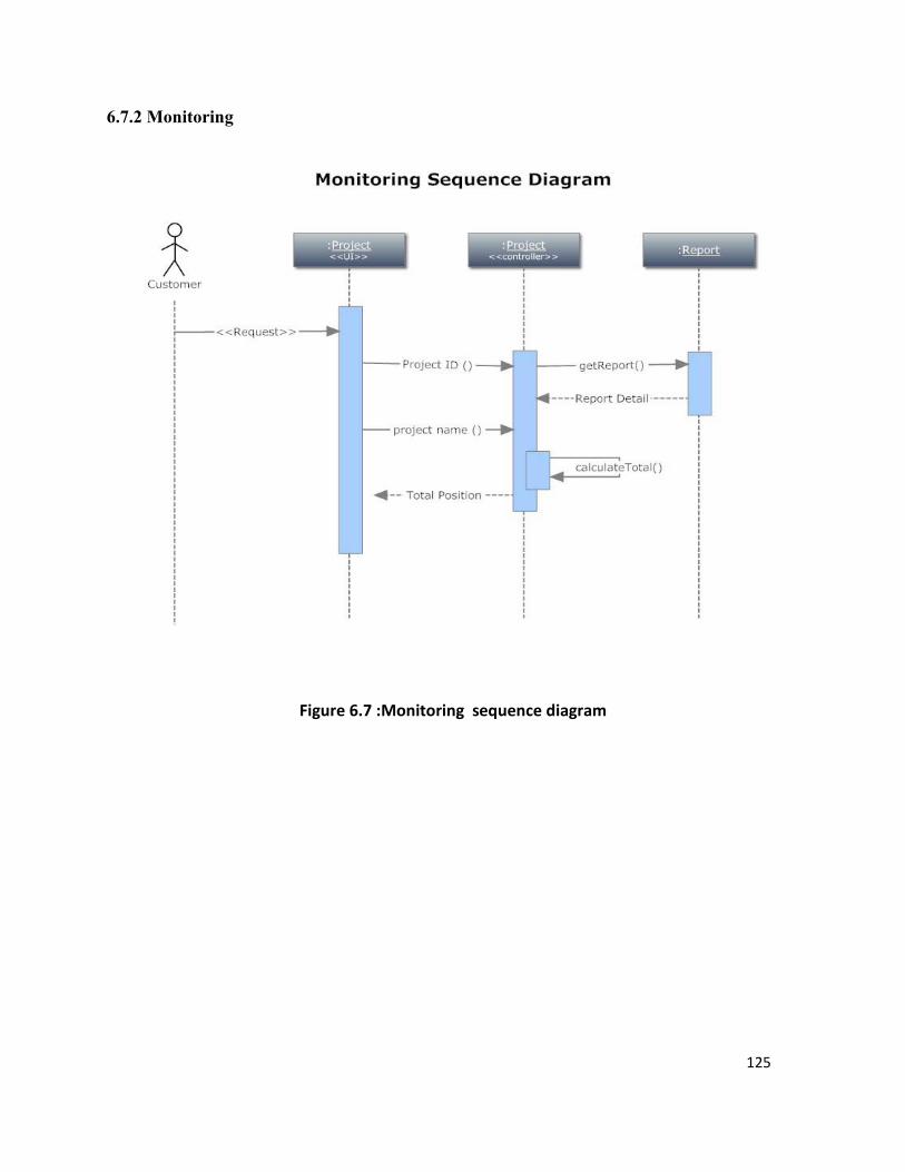
125
6.7.2 Monitoring
Figure 6.7 :Monitoring sequence diagram

126
6.7.3 Calculability
Figure 6.8: Calculation sequence diagram
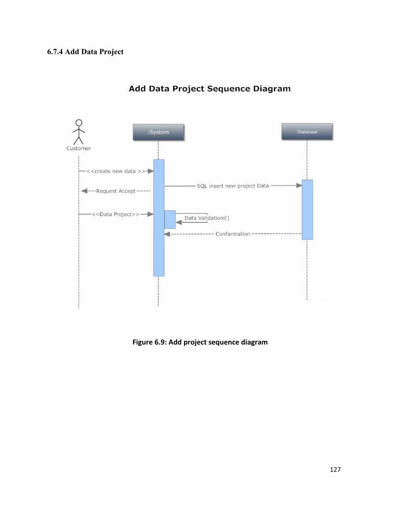
127
6.7.4 Add Data Project
Figure 6.9: Add project sequence diagram

128
6.7.5 Add Depot
Figure 6.10: Add Depot sequence diagram

129
6.7.6. Add Report
Figure 6.11 :Add report sequence diagram

130
6.8 Database Design
The Database Design of the proposed DSS is explained by means of an Entity and Relationship
Diagram (Figure 6.12).
Figure 6.12 :Entity and Relationship diagram

131
6.9 Interfaces
6.9.1 User Interfaces
Users interact with the system using forms and buttons. Figure 6.13 presents the various forms
associated with user interface of the proposed DSS.
User interface Login Screen: This is for the Administrator to get into the software. It requires a
user name and password.
Project Details: This shows the project status of various reports with their results.
New Registrations: This utility is to create new project or clients in the system.
Reports: This utility is used to generate various reports of project in different steps of
calculation.
User Login (Client Side): The user has to give a username and password by which he or she can
access the software.
Password Form
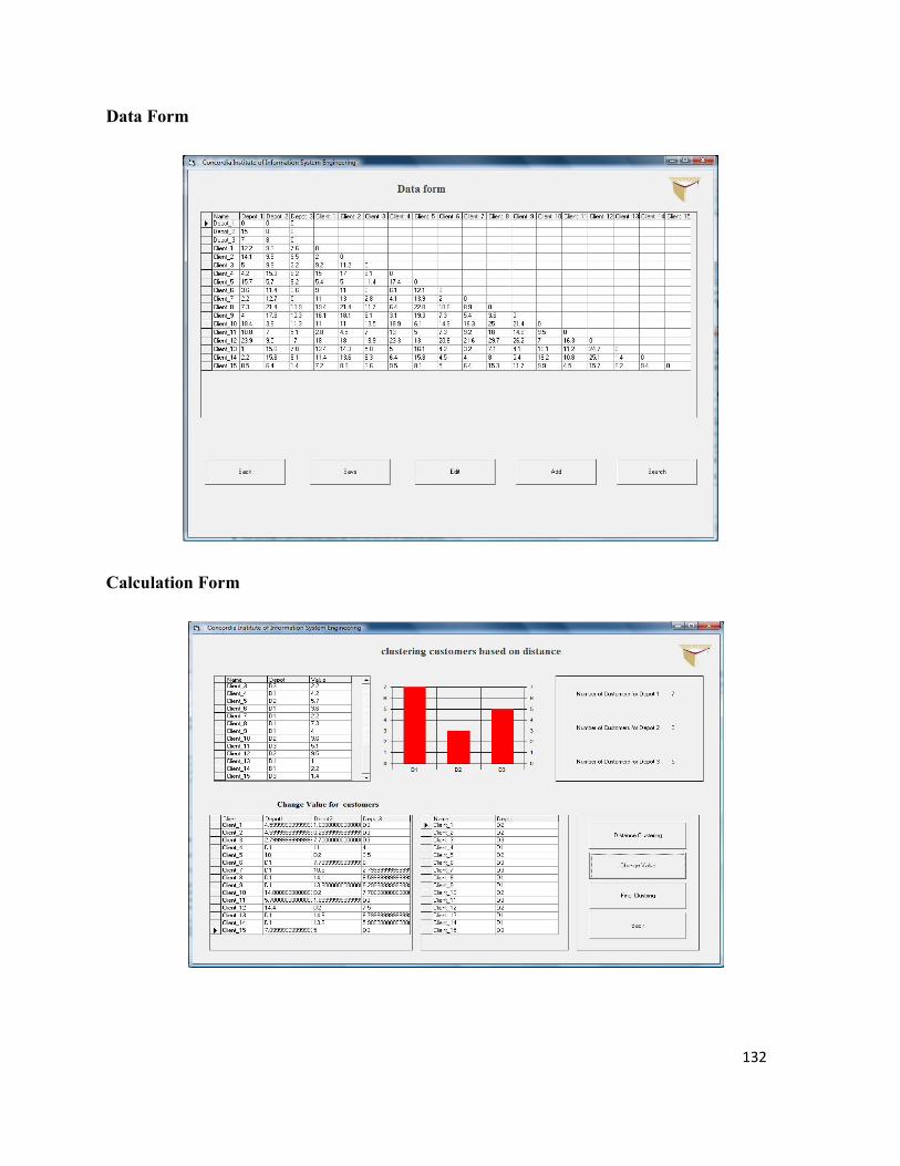
132
Data Form
Calculation Form

133
Scheduling form
Chart Form
Figure 6.13: User Interfaces
134
6.9.2 Hardware Interfaces
The server is connected to the client systems. Also, the client has access to the database for
accessing the project details. The client’s access to the database in the server is read only.
6.9.3 Software Interfaces
Software interfaces is a multi-user, multi-tasking environment.
6.9.4 Communications Interfaces
Communication interfaces of the Goods Distribute System uses SQL Connection and Java
Applets and hence requires HTTP for transmission of data or local LAN.
6.10 Testing Results
Software testing is any activity aimed at evaluating an attribute or capability of a program or
system and determining that it meets its required results. Testing is more than just debugging.
The purpose of testing can be quality assurance, verification and validation, or reliability
estimation. Testing can be used as a generic metric as well, so in this project we have to test all
the use cases of the system.
6.10.1 Software result
Based on the process method and the results of the software, we found the software method
including clustering, scheduling and routing for Distribute System Allocation and the software
is practical and could be executive (or executed?) in actual business activities or supply chain
management. Besides, other critical factors for business play a key role in the efficiency of
delivery process.

135
Chapter 7:
Conclusions and future works
7.1 Summary
Efficient distribution of goods is critical in maximizing revenues of logistics companies and
minimizing environmental impacts on city residents and their environment. In this thesis, we
address the problem of goods distribution planning in urban areas and propose a three step
approach to address the following problems:
Balanced allocation of customers to logistics depots
Order scheduling of customers at logistics depots
Vehicle allocation and route planning for goods distribution to customers
In the first step, we propose an integrated approach based on Nearest Neighbour and Tabu
Search for balanced allocation of customers to logistics depots under congestion, access and
timing regulations of the city. The objective is to minimize transportation costs subject to
capacity constraints of logistics depots.
In the second step, we perform order scheduling for the customers allocated to each logistic
depot using Genetic algorithms. The objective is to minimize distribution costs while respecting
the time window constraints of customers, their order priorities, and any time or access
regulation imposed by the municipal administration in the city.

136
In the third and the last step, we apply modified Dijkstra’s algorithm to calculate fastest paths for
goods delivery to customer considering the presence of congestion, road incident and road type.
The proposed approaches are tested and validated by comparison against other standard
approaches available in literature.
7.2 Advantages
Integrating the above three approaches, a prototype decision support system is developed for
goods distribution planning in urban areas. The strength of the proposed work is its ability to
deal with large size problem sets and generate fast, good quality solutions for goods distribution
to customers. We also design and suggest better ways of efficiently distributing goods to cities,
taking into consideration the city traffic condition, as well as access-timing-sizing regulations
imposed by municipal administration in urban areas.
7.3 Limitations
The main limitation of our work is the lack of real time information on traffic conditions and
vehicle availabilities during the planning process. Also, we have covered the last link of supply
chain namely from depots (retailers) to clients, however, the ideas of the proposed work can be
extended for application to other levels of supply chain networks.
7.4 Future Works
The next step of our work involves the following
Managing immediate customer demands in routing and scheduling

137
Congestion modelling
Investigating the application of Intelligent Transportation Systems for data collection for
efficient goods distribution planning
Testing and validating the proposed goods distribution software for large problem
instances.

138
Chapter 8:
References
1. Aikens C.H. (1985), Facility location models for distribution planning, European Journal
of Operational Research, 22, 263–279.
2. Anderson, S., Allen, J. and Browne, M. (2005) Urban logistics: how can it meet policy
makers’ sustainability objectives?, Journal of Transport Geography 13 (1), 71–81.
3. Badran M.F., El-Haggar S.M. (2006), Optimization of municipal solid waste
management in Port Said–Egypt, Waste Management, 26(5), 534-545.
4. Baker E. K. (1983), An Exact Algorithm for the Time-Constrained Traveling Salesman
Problem, Operations Research, 31(5), 938-945.
5. Baita F, Pesenti R, Ukovich W, Favaretto D (1998), A comparison of different solution
approaches to the vehicle scheduling problem in a practical case, Trieste, Italy.
6. Basnet, C., L. R. Foulds, Wilson J. M. (1999), Heuristic for vehicle routing on tree-like
networks, Journal of Operational Research Society, 50(6), 627-635.
7. Berger, J., Mohamed B., (2003), A hybrid genetic algorithm for the capacitated vehicle
routing problem, Proc. of the Genetic and Evolutionary Computation Conference,
Chicago, 646-656.
8. Bianchi L., Birattari M., Chiarandini M., Manfrin M., Mastrolilli M., Paquete L., Rossi
Doria O., Schiavinotto T. (2004), Metaheuristics for the vehicle routing problem with
stochastic demands. Technical Report TR-12-04, IDSIA, Galleria 2, Manno, 6928,
Switzerland.

139
9. Bramel, J. B., Simchi-levi D. (1995), A location based heuristic for general routing
problems, Operations Research, 43(4), 649-660.
10. Braysy, I. and Gendreau, M. (2005). Vehicle routing problem with time windows, part II:
Metaheuristics. Transportation Science, 39(1), 119-139.
11. Browne, M. and Allen. J. (1999) The impact of sustainability policies on urban freight
transport and logistics systems. 8th World Conf. Transport Res. _WCTR_, Antwerp,
Belgium. Elsevier, Amsterdam, 505–518.
12. Brugge R. (1991) Logistical developments in urban distribution and their impact on
energy use and the environment, in: Freight transport and the environment, 331-342,
Elsevier Science Publishers, Amsterdam.
13. Campbell, A.M., Savelsbergh, M. (2005). Efficient insertion heuristics for vehicle routing
and scheduling problems. Transportation Science, 38(3), 369-378.
14. Chan F.T.S., Kumar N. (2009), Effective allocation of customers to distribution centres: a
multiple ant colony optimization approach. Robotics Computer-Integrated
Manufacturing, 25(1), 1–12.
15. Chen J.S. (2010), Integration of Order Scheduling with Delivery Vehicles Routing for
Two-Echelon Supply Chain System, 7th International Conference on Service Systems
and Service Management (ICSSSM), pp 1 - 4 , Tokyo, ISBN: 978-1-4244-6485-4
16. Chen Z, Jiang C. (2004), A Reseau-Dividing Algorithm for Distributing Products of
Hangzhou Tobacco Company, Systems Engineering -Theory & Practice, 24 (3), 46-51.

140
17. Cheung, B.K.S., Choy K.L., Li C.L., Shi W., Tang J., (2008), Dynamic routing model
and solution methods for fleet management with mobile technologies, International
Journal of Production Economics, 113(2), 694-705.
18. Chien T. W. (1993), Determining profit-maximizing production/shipping policies in a
one-to-one direct shipping, stochastic demand environment. European Journal of
Operational Research, 64(1), 83-102.
19. Christofides A,. Mingozzani D, Toth P. (1979), The Vehicle Routing Problem. In
Combinatorial Optimizations, N. Christofides, R. Mingozzi, P. Toth,and C. Sandi (eds.).
John Wiley & Sons, New York.
20. Clarke G., Wright J.W. (1964), Scheduling of Vehicles from A Central Depot to A
Number of Delivery Points, Operations Research, 12(4), 568-581.
21. Cormen, Thomas H.; Leiserson, Charles E.; Rivest, Ronald L.; Stein, Clifford (2001).
"Section 24.3: Dijkstra's algorithm". Introduction to Algorithms (Second ed.). MIT Press
and McGraw-Hill, 595–601. ISBN 0-262-03293-7.
22. Crainic, T. G. , Ricciardi, N. and Storchi, G. (2007) Models for Evaluating and Planning
City Logistics Transportation Systems, CIRRELT-2007-65, CIRRELT Report,
University of Montreal, Montreal.
23. Dablanc, L. (2007), Goods transport in large European cities: Difficult to organize,
difficult to modernize, Transportation Research A, 41, 280-285.
24. Dijkstra, E. W. (1959). "A note on two problems in connexion with graphs". Numerische
Mathematik, 1, 269–271. doi:10.1007/BF01386390.

141
25. Dondo R., Cerda J. (2007), A cluster-based optimization approach for the multi-depot
heterogeneous fleet vehicle routing problem with time windows, European Journal of
Operational Research, 176, 1478-1507.
26. Dror M., Trudeau P., (1989), Savings by split delivery routing, Transportation Science,
23, 141-145.
27. Eglese, R.W., Mercer A., Sohrabi B., (2005), The grocery superstore vehicle scheduling
problem, Journal of the Operational Research Society, 56(8), 902-911.
28. Eriksson J.R., Svensson T. (2008), Efficiency in goods distribution collaboration in cities
- SAMLIC, VTI report 623A, 1-36.
29. Faccio M., Persona A., Zanin G. (2011), Waste collection multi objective model with real
time traceability data, Waste Management, 31(12),2391-2405.
30. Fazel-Zarandi M.M., Christopher Beck J., (2009), Solving a Location-Allocation
Problem with Logic-Based Benders' Decomposition, CP'09 Proceedings of the 15th
international conference on Principles and practice of constraint programming, Springer-
Verlag Berlin, Heidelberg, ISBN:3-642-04243-0 978-3-642-04243-0.
31. Fisher, M. L., Jaikumar, R. (1981), A generalized assignment heuristic for vehicle
routing, Networks, 11(2), 109-124.
32. Fleischmann, B., Gietz M., Grutzmann, S. (2004), Time-varying Travel Times in Vehicle
Routing, Transportation Science, 38(2), 160-174.
33. Fu, L., Rilett, L.R. (1998), Shortest path problems in traffic networks with dynamic and
stochastic link travel times, Transportation Research B, 32(7), 499-516.

142
34. Fu, L.(2002), Scheduling dial-a-ride paratransit under time-varying stochastic congestion,
Transportation Research B, 36(6), 485-506.
35. Funke, B., Grunert, T., Irnich, S. (2005). Local search for vehicle routing and scheduling
problems: Review and conceptual integration. Journal of Heuristics, 11(4), 267-306.
36. Gaskell, T.J. (1967), Bases for vehicle fleet scheduling, Operation Research, 18(3), 281-
295.
37. Ghandforoush, P., Sen, T. K.(2010), A DSS to manage platelet production supply chain
for regional blood centers ,Decision Support Systems, 50(1), 32-42.
38. Glover, F., Laguna, M. (1997), Tabu search. Kluwer academic publishers.
39. Hu, X., Huang, M. (2007), An intelligent solution system for a vehicle routing problem in
urban distribution, International Journal of Innovative Computing, 3(1), 189-198.
40. Huang, B., Liu, N. (2004) Bilevel programming approach to optimizing a logistic
distribution network with balancing requirements. Transportation Research Record, No.
1894, TRB. National Research Council, Washington, D.C., 188–197.
41. Ho, S.C., Haugland, D. (2002), A Tabu Search Heuristic for the Vehicle Routing Problem
with Time Windows and Split Deliveries, University of Bergen N-5020 Bergen, Norway.
42. Ichoua, S., Gendreau, M., Potvin, J.Y. (2003), Vehicle dispatching with time-dependent
travel times, European Journal of Operational Research, 144, 379-396.
43. Jaumard, B., Semet, F., Vovor, T. (1998), A generalized linear programming model for
nurse scheduling, European journal of operational research 107, 1-18.

143
44. Kim, S., Lewis, M.E., White, C.C. (2005), Optimal Vehicle Routing with Real-Time
Information, IEEE journal on Intelligent Transportation Systems, 6(2), 178-188.
45. Kleywegt, A. J., Nori, V. S., Savelsbergh, M. W. P. (2002), The stochastic inventory
routing problem with direct deliveries. Transportation Science, 36(1), 94-118.
46. Laporte, G. (1992), The traveling salesman problem: An overview of exact and
approximate algorithms, European Journal of Operational Research, 59(2), 231-247.
47. Li, N., Wang, S., Li, Y. (2011), A Hybrid Approach of GA and ACO for VRP, Journal of
Computational Information Systems, 7(13), 4939-4946.
48. Li, J-Q, Borenstein, D., Mirchandani, P.B. (2008), Truck scheduling for solidwaste
collection in the City of Porto Alegre, Brazil, Omega, 36, 1133–1149.
49. Liu, C.M. , Chang, T.C. (2006), Multi-objective heuristics for the vehicle routing
problem, International Journal of Operations Research, 3(3), 173-181.
50. Lu, Y., Yang, Y., Lu, F. (2006), Optimal vehicle routing problem based on fuzzy
clustering analysis. Journal of Jilin University (Engineering and Technology Edition),
36(9), 147-151.
51. Maden, W., Eglese, R., Black, D. (2009), Vehicle routing and scheduling with time-
varying data: A case study, Working paper, Department of Management Science,
Lancaster University Management School, Lancaster, UK.
52. Min, H., Zhou, G., Gen, M., Cao, Z. (2005) A genetic algorithm approach to the balanced
allocation of customers to multiple warehouses with varying capacities, International
Journal of Logistics Research & Applications, 8(3), 181–192.

144
53. Montemanni, R., Gambardella, L. M., Rizzoli, A. E., Donati, A. V. (2005), Ant Colony
System for a Dynamic Vehicle Routing Problem, Journal of Combinatorial Optimization,
10(4), Publisher: Springer Netherlands, 327-343.
54. Muñuzuri, J. Larraneta, J. Onieva, L., Cortes, P. (2005) Solutions applicable by local
administrations for urban logistics improvement, Cities 22 (1), 15–28.
55. Nikolakopoulou, G., Kortesis, S., Synefaki, A., Kalfakakou, R. (2004). Solving a vehicle
routingproblem by balancing the vehicles time utilization, European Journal of
Operational Research, 152(2), 520-527.
56. Nuortio, T., Kytöjoki, J., Niska, H., Bräysy, O. (2006), Improved route planning and
scheduling of waste collection and transport, Expert Systems with
Applications, 30(2), 223-232.
57. Ogden, K.W. (1992), Urban goods movement: a guide to policy and planning, Ashgate,
Aldershot, England, 397, ISBN 1-85742-029-2.
58. Osvald, A., Stirn, L. Z. (2008), A vehicle routing algorithm for the distribution of fresh
vegetables and similar perishable food, Journal of Food Engineering, 85(2), 285-295.
59. Park B. J., Choi H. R., Kim H. S. (2003), A hybrid genetic algorithm for the job shop
scheduling problems, Computers & Industrial Engineering, 45, 597–613.
60. Polimeni, A., Vitetta, A. (2010), Demand and routing models for urban goods movement
simulation ,12th WCTR, Lisbon, Portugal
http://intranet.imet.gr/Portals/0/UsefulDocuments/documents/01329.pdf
61. Potvin, J.Y., Xu, Y, Benyahi, I.(2006), Vehicle routing and scheduling with dynamic
travel times, Computers & Operations Research, 33, 1129–1137.

145
62. Powell, W.B. (1990), Real-time optimization for truckload motor carriers, OR/MS
Today, 18, 28-33.
63. Quak, H. J. and De Koster, M. B. M. (2009) Delivering goods in urban areas: How to
deal with urban policy restrictions and the environment, Transportation Science, 43(2),
211–227.
64. Rajesh, R., Pugazhendhi, S., Ganesh, K. (2011), Simulated annealing algorithm for
balanced allocation problem, The International Journal of Advanced Manufacturing
Technology, 1-10.
65. Reimann, M., Doerner, K., Hartl R. F. (2004), D-ants: Savings based ants divide and
conquer the vehicle routing problem, Computers & Operations Research, 31(4), 563-591.
66. Ren Y. (2011), Metaheuristics for capacitated location allocation problem on logistics
networks, MASc thesis, Concordia University.
67. Ruiz, R., Moroto, C., Alcaraz, J. (2004). A decision support system for a real vehicle
routing problem. European Journal of Operational Research, 153(3), 593-606.
68. Savelsbergh M.W.P., Sol M. (1997), Drive: Dynamic routing of independent vehicles,
Operations Research, 46474-490.
69. Shahzad F., Tenti F.M. (2009), Efficient Distribution Systems for goods to the City
centre, Master Degree Project No. 2009:46, University of Gothenburg, Sweden.
70. Slater A., (2002) Specification for a dynamic vehicle routing and scheduling system,
International Journal of Transportation Management 1, 29-40.
71. Solomon M. (1997), Algorithms for the vehicle routing and scheduling problems with
time window constraints. Operations Research, 35, 245–265.

146
72. Sun, L., Hu, X., Wang, Z. (2006), Reviews on Vehicle Routing Problem and Its Solution
methods. Systems Engineering, 11, 35-41.
73. Taillard E.D., Badeau P., Gendreau M., Guertin F., Potvin J.Y. (1997), A tabu search
heuristic for the vehicle routing problem with soft time windows, Transportation Science,
31, 170–186.
74. Taniguchi E., Shimamoto H. (2004). Intelligent transportation system based dynamic
vehicle routing and scheduling with variable travel times, Transportation Research C, 12,
235–250.
75. Taniguchi, E. (2000) City Logistics: Network Modeling and Intelligent Transport
Systems, Amsterdam, London: Pregamon.
76. Teng, S.Y., Ong, H.L., Huang, H.C. (2003). A comparative study of metaheuristics for
vehicle routing problem with stochastic demands. Asia-Pacific Journal of Operational
Research, 20(1): 103-119.
77. Toth, P., Vigo, D. (2003). The granular tabu search and its application to the vehicle
routing problem. INFORMS Journal on Computing, 15, 333–346.
78. Visser, J., Van Binsbergen, A., and Nemoto, T. (1999) Urban freight transport policy and
planning. City Logistics 1, 1-35.
79. Yang J. (2005), The complexity of customer order scheduling problems on parallel
machines, Computers and Operations Research, 32, 1921–1939.
80. Yang J., Jaillet P., Mahmassani H. (1999), On-Line Algorithms for Truck Fleet
Assignment and Scheduling under Real-Time Information, Transportation Research
Record, 1667, 107-113.

147
81. Zeimpekis V., Tatarakis A., Giaglis G.M., Minis I. (2007), Towards a Dynamic Real-
Time Vehicle Management System for Urban Distribution, International Journal of
Integrated Supply Management, 3(3), 228-243.
82. Zhan, F. B., Noon, C. E. (1998), Shortest Path Algorithms: An Evaluation Using Real
Road Networks, Transportation Science 32 (1), 65–73. doi:10.1287/trsc.32.1.65.
83. Zhou G., Min H., Gen M , (2002), The balanced allocation of customers to multiple
distribution centers in the supply chain network: a genetic algorithm approach,
Computers and Industrial Engineering archive, 43(1-2), 251 – 261.