a decision making approach for multi-objective

178 ECTI TRANSACTIONS ON COMPUTER AND INFORMATION TECHNOLOGY VOL.11, NO.2 November 2017

A Decision Making Approach forMulti-Objective Optimization Considering A

Trade-Off Method

Tipwimol Sooktip1 and Naruemon Wattanapongsakorn2

ABSTRACT

In multi-objective optimization problem, a set ofoptimal solutions is obtained from an optimizationalgorithm. There are many trade-off optimal solu-tions. However, in practice, a decision maker or useronly needs one or very few solutions for implemen-tation. Moreover, these solutions are difficult to de-termine from a set of optimal solutions of complexsystem. Therefore, a trade-off method for multi-objective optimization is proposed for identifying thepreferred solutions according to the decision maker’spreference. The preference is expressed by using thetrade-off between any two objectives where the deci-sion maker is willing to worsen in one objective valuein order to gain improvement in the other objectivevalue. The trade-off method is demonstrated by usingwell-known two-objective and three-objective bench-mark problems. Furthermore, a system design prob-lem with component allocation is also considered toillustrate the applicability of the proposed method.The results show that the trade-off method can beapplied for solving practical problems to identify thefinal solution(s) and easy to use even when the deci-sion maker lacks some knowledge or not an expertin the problem solving. The decision maker onlygives his/her preference information. Then, the corre-sponding optimal solutions will be obtained, accord-ingly.

Keywords: Multi-Objective Optimization, DecisionMaking Approach, Preference-Based Method, Trade-Off Method

1. INTRODUCTION

Most real-life optimization problems have severalfactors or objectives to be optimized simultaneously.These problems can be expressed as multi-objectiveoptimization problems. In the problems, the objec-tive functions may be conflicting with each other. Forexample, the objectives are to maximize system per-

Manuscript received on September 13, 2017 ; revised on De-cember 9, 2017.Final manuscript received on December 9, 2017.1,2 The authors are with Department of Computer En-

gineering, King Mongkut’s University of Technology Thon-buri, 126 Pracha-Uthit Rd., Bangmod, Thoongkhru, Bangkok10140, Thailand, E-mail: [email protected] and [email protected]

formance but minimize system cost simultaneously.Due to the conflicting objective functions, the op-timal solutions have trade-off among the objectiveswhich means a losing value in one objective whilegaining value in other objective in return. Therefore,it is difficult for a Decision Maker (DM) or user toselect one final solution. In other words, the problemsolving becomes challenging because it contains manytrade-off optimal solutions but only one solution willbe selected for implementation. Hence, the user needsa solving method for helping him/her makes a deci-sion and gets the most desirable or outstanding solu-tion(s).

For solving multi-objective optimization problems,most multi-objective optimization researches concen-trate on searching for the optimal solutions set. How-ever, the DM still needs to choose the final solutionfor implementation as has been described. There-fore, we are interested in identifying methods forthe most preferred solution. The preference-basedmethod becomes more important. Many researches[1-5] showed that the preference-based optimizationmethods are effective to guide the optimization algo-rithm toward the preferred regions and identify themost preferred solution. There are many ways toexpress the DM’s preferences including the referencepoint methods [6-8], a light beam search method [9-10] and a dynamic polar-based region [11]. However,we focus on compromising trade-off between any twoobjectives. The objective trade-offs concept is pre-sented in [12]. The trade-off concept represents theeffect of changing between two alternative solutions.J. Branke et al. [13] presented a method that mod-ified the definition of dominance according to linearmaximum and minimum trade-off functions for eachpair of objectives. Tilahun and Ong [14] proposedthe fuzzy preferences incorporated with genetic al-gorithm for multiple DMs. This method collectedpreferences as fuzzy conditional trade-offs. However,it is not easy for the DM to specify trade-off for ev-ery alternative. Therefore, we developed the trade-offpreference-based method in order to help identifyingpreferred solution(s) even when the DM is not an ex-pert in the problem solving.

In this research, the trade-off method accord-ing to the extreme solution is proposed. It is apreference-based method to identify the most pre-ferred/outstanding solution(s) among multiple opti-

A Decision Making Approach for Multi-Objective Optimization Considering A Trade-Off Method 179

mal solutions. The DM’s demand can easily be ex-pressed and maintained.

This paper is organized as follows. The next sec-tion describes multi-objective optimization problem.Then, the preference-based methods are presented inSection 3. Section 4 proposes a trade-off methodaccording to the extreme solution. The benchmarkproblems are presented in Section 5., followed by theapplication problem, component allocation problem,in Section 6. The simulation results and discussionare presented in Section 7. Lastly, Section 8 givesconclusion.

2. MULTI-OBJECTIVE OPTIMIZATION

Multi-objective optimization is determining thedecision variable(s) that optimize multiple objectivessimultaneously under the constraints. For exam-ple, the objectives of system design are maximiz-ing system performance while minimizing system costand weight subject to system constraints. Decisionvariable(s) is represented by a n dimensional vec-tor, x = (x1, x2, . . . , xn)

T where n is the numberof decision variable(s). The objective functions aref1(x), f2(x), . . . , fM (x) where M is the number of ob-jective functions. The objective function can be min-imized or maximized. The mathematical formulationof the MOP in general format (1) is following [15]:Maximize/Minimize f1(x), f2(x), . . . , fM (x)

Subject to gj(x) = 0, j = 1, 2, . . . , J ;hk(x) = 0, k = 1, 2, . . . ,K;

x(L)i ≤ xi ≤ x

(U)i ,

i = 1, 2, . . . , n. (1)

where the gj(x) and hk(x) functions are the con-straint functions which have J inequality constraintfunctions and K equality constraint functions. The

variable boundary is the last set of constraints (x(L)i ≤

xi ≤ x(U)i ), where the decision variable, xi has a lower

bound, x(L)i and an upper bound, x

(U)i The objective

function may be in conflict with each other and causesmultiple trade-off solutions.Multi-objective optimization problem can be solvedefficiently by using well-known multi-objective evo-lutionary algorithms such as SPEA2 [16], Non-dominated Sorting Genetic Algorithm (NSGA-II) [17]and MOEA/D [18]. These algorithms can be used inorder to obtain an approximation of Pareto-optimalsolutions. Then, the preferred solution is identi-fied/selected by using the proposed method, as thefinal solution for implementation. The well-knownoptimization method, NSGA-II [17] is used in thisresearch according to its effectiveness.

3. PREFERENCE-BASED METHOD

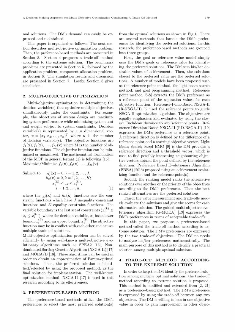
The preference-based methods utilize the DM’spreferences to select the most preferred solution(s)

from the optimal solutions as shown in Fig 1. Thereare several methods that handle the DM’s prefer-ences for identifying the preferred solutions. In thisresearch, the preference-based methods are groupedinto three groups.

First, the goal or reference value model simplyuses the DM’s goals or reference value for identify-ing the preferred solutions. The DM sets his/her de-sirable values of achievement. Then, the solutionsclosest to the preferred value are the preferred solu-tions. A number of models have been proposed suchas the reference point method, the light beam searchmethod, and goal programming method. Referencepoint method [6-8] extracts the DM’s preference asa reference point of the aspiration values for eachobjective function. Reference-Point-Based NSGA-II(R-NSGA-II) [6] used the reference points to guideNSGA-II optimization algorithm. The objectives areequally emphasizes and evaluated by using the clos-est Euclidean distance to any reference points. Ref-erence Direction Based NSGA-II (RD-NSGA-II) [19]expresses the DM’s preference as a reference point.A reference direction is defined by the difference of areference point and a starting objective vector. LightBeam Search based EMO [9] is the DM provides areference direction and a threshold vector, which isused to find possibly interesting neighbouring objec-tive vectors around the point defined by the referencedirection. Preference Based Evolutionary Algorithm(PBEA) [20] is proposed using an achievement scalar-izing function and the reference point(s).

Second, the ranking model ranks the alternativesolutions over another or the priority of the objectivesaccording to the DM’s preferences. Then the bestranked alternatives are the preferred solutions.

Third, the value measurement and trade-offs mod-els evaluate the solutions and give the scores for eachalternative solution. The guided multi-objective evo-lutionary algorithm (G-MOEA) [13] expresses theDM’s preferences in terms of acceptable trade-offs.

In this paper, we propose a preference-basedmethod called the trade-off method according to ex-treme solution. The DM’s preferences are expressedby the two trade-off objectives. The DM no needsto analyse his/her preferences mathematically. Themain purpose of this method is to identify a practicalsolution among multiple optimal solutions.

4. TRADE-OFF METHOD ACCORDINGTO THE EXTREME SOLUTION

In order to help the DM identify the preferred solu-tion among multiple optimal solutions, the trade-offmethod according to extreme solution is proposed.This method is modified and extended from [2, 21]as a preference-based method. The DM’s preferenceis expressed by using the trade-off between any twoobjectives. The DM is willing to loss in one objectivevalue in order to gain improvement in other objec-


Fig.1: The concept of a preference-based method anda preferred solution.

tive value. For an example, sacrificing or paying 1unit of cost so that some units of product can begained. An optimization method finds the approxi-mation of Pareto front before the proposed methodidentifies the preferred solutions. In this research,we use NSGA-II [17] which is a well-known multi-objective evolutionary optimization method. Afterobtaining an approximation of the optimal solutionsfrom the optimization method, the proposed methodidentifies the preferred solution set and presents it tothe DM. The flowchart of trade-off method is shownin Fig 2. The process of the trade-off method by usingextreme solution as reference solution is as follows.

Step 1: The DM specifies preference information.The DM specifies gaining objective value (hopefullyto get the better value) and sacrificing the other ob-jective (willing to pay more or get worst). In thisresearch, the sacrifice in system cost is related to thegain in system reliability which means the user is will-ing to accept higher system cost (sacrificing objective)in order to increase system reliability (gaining objec-tive).

Step 2: Normalize the objective valuesAll objective functions are scaled to be in the rangefrom 0.0 to 1.0. The normalized objective value isgiven by:

Normalized(fi(x)) =fi(x)− fmin

i

fmaxi − fmin

i

(2)

i = 1, 2, . . . , b.

where x is a set of the decision variables. The num-ber of objective functions is b. In the approximationof optimal solutions, fmax

i and fmini are the maxi-

mum and the minimum values for the ith objectivefunction, fi(x), respectively.

Fig.2: Flowchart of Trade-off method according tothe extreme solution.

Step 3: Select the extreme solution as a reference.The solution that has extremely good value in sacri-ficing objective (system cost) is selected as a referencesolution. If there is more than one solution, choosethe solution among them that has the best value ingaining objective (system reliability).

Step 4: Eliminate unimproved solutions.Eliminate solutions that have gaining objective valuenot as good as that of the reference solution.

Step 5: Calculate the preferred scoreThe preferred score is the trade-off value of the solu-tion k and reference solution which is given by:


T kij =

|f reference solutionj (x)− fk

j (x)||f reference solution

i (x)− fki (x)|

(3)

where the decision variable vector is x. The T kij rep-

resents the amount of gaining in the objective j, fj tosacrifice one unit in the objective i, fi of solution k.There is no need to calculate score for the referenceand eliminated solutions.Step 6: Sort the preferred solutionSolution with the highest score is the most preferredsolution. The alternative that has the highest pre-ferred score means that it has the maximum amountto gain in one objective when compare to the extremereference solution.Step 7: Present the preferred solutionPresent appropriate solutions to the DM. The processis completed if the DM satisfies them.Step 8: If the DM does not satisfy with the preferredsolution, he/she specifies an acceptable value.Step 9: Eliminate unacceptable solutionsEliminate solutions that gaining objective value is notas good as the acceptable value. Then repeat steps6 to 9. Among the remaining solutions, solution thathas the highest preferred score is the most preferredsolution.The main contribute in this research is to help theDM express the trade-off preference easily and moreflexibility in order to find the final solution.

5. BENCHMARK PROBLEMS

The preference-based methods for pruning mech-anism have different ways to express the DM’s pref-erence. Thus, it is difficult to compare the resultsdirectly among the different preference-based meth-ods. The preference-based methods focus on the mostdesirable solutions. However, many multi-objectivebenchmark problems have been proposed to evaluatethe algorithms. The benchmark problem is used toevaluate the ability and tests the effectiveness of apreference-based method with known non-dominatedsolutions.

The common benchmark problems are includingZitzler-Deb-Thiele test problems (ZDT) [22] test suiteand Walking-Fish-Group (WFG) test problems [23].ZDT test suite is the most popular used in the multi-objective optimization. ZDT problems consist of sixbi-objective problems. The characteristics of testproblems include concave, convex, continuous anddiscontinuous problems. WFG is scalable to anynumber of parameters and objectives and have morecomprehensive challenges among other test suite [23].The mathematical models are presented as the follow-ing.

5.1 Two-Objective Benchmark Problems

The ZDT test problems [22] consist of six problems in-cluding ZDT1 to ZDT6. ZDT test problem suite has

two objectives to be minimized. This research consid-ers all ZDT problems except ZDT4 because the ZDT4has similar PF as ZDT1. The ZDT problem suite pro-vides sufficient complexity to compare the preferredsolution on various shape of Pareto front where theconcave, convex, continuous and discontinuous shapeof Pareto front are the problem features that causesdifficulty for identifying the preferred solutions.

5.2 Three-Objective Benchmark Problems

For three-objective problem, we consider WFG23D from WFG test problems [23]. The characteris-tics of WFG2 3D test problem include convex, discon-tinuous and multimodal as shown in Fig 6 (a). Themathematical model is presented as the following [23,24].

Minimize:fm=1:m−1(x⃗) = xM + SMconvexm(x1, . . . , xM−1)

fm(x⃗) = xM + SMdiscm(x1, . . . , xM−1)

whereyi=1:M−1=r sum(

[y

′ (i−1)k(M−1)+1, . . . , y

′ ik(M−1)

], [1, . . . , 1])

ym=r sum([y

′

k+1, . . . , y′

k+l/2

], [1, . . . , 1])

y′

i=1:k=y′′

i

y′

i=k+1:k+l/2=r nonsep([y

′′

k+2(i−k)−1, y′′

k+2(i−k)−1

], 2)

y′

i=1:k = zi,[0,1]y

′′

k+1:n=s linear(zi,[0,1], 0.35)

where M is the number of objectives and z are thedecision variables. Sm is a constant to modify posi-tion and scale for the optimal solutions of objectivemth. i and m are the indices. k is a position-relatedparameter. l is a distance-related parameter.

Transformation function:r sum is the weighted sum reduction transformationfunction.r nonsep is the non-separable reduction transforma-tion function.s linear is the linear shift transformation function.

Shape function:convex is the convex shape function.disc is the disconnected shape function.

6. APPLICATION PROBLEM: COMPO-NENT ALLOCATION PROBLEM

The component and redundancy allocation prob-lem is to optimize a system design by allocating re-dundant components from the design alternatives.This research considers a series-parallel system, theindependent alternative component and mixing ofnon-identical components. The system structure isshown in Fig 3.


Fig.3: General series-parallel redundancy system.

The problem is a well-known NP-hard problem [25]which is difficult to solve within a reasonable time.The mixing of non-identical components is allowed ineach subsystem causing many possible alternative so-lutions and also giving a large set of optimal solutions.Therefore, it is difficult to identify the preferred so-lutions. The system and components have only twostates: work or fail while the component failure isstatistically independent. The example solution forsmall system design is shown in Fig 4, where subsys-tem 1 has one component type A while subsystem 2has one component type B, and subsystem 3 has onecomponent type A together with one of type C.

Fig.4: Example of small system design problem.

The objective functions of system design problem areas follows [21, 25, 26].

Objective 1: Maximize system reliability (Rsys)

maxRsys(x) =∏m

i=1Ri(xi) (4)

Objective 2: Minimize system cost (Csys)

minCsys(x) =

m∑i=1

ti∑j=1

cijxij (5)

Objective 3: Minimize system weight (Wsys)

minWsys(x) =m∑i=1

ti∑j=1

wijxij (6)

The system constraints are as follows.

1 ≤ti∑

j=1

xij ≤ nmax

Ri(x) = 1−∏ti

j=1(1−Rij(x))

xij

0 ≤ Rij(x) ≤ 1

xij ∈ {0, 1, 2, . . . , nmax}, i = 1, 2, . . . , m and j = 1,2, . . ., ti

where the number of components of type j in sub-system i is xij while x, xi are the vector of xij . Ri

is the reliability of subsystem i. The reliability, costand weight of the jth component in subsystem i rep-resented by rij , cij and wij , respectively are givenas input data for component allocation alternatives.The designed system is composed of m subsystemsconnected in series. The number of allocated compo-nents connected in parallel in subsystem i is ti. Themaximum number of components in subsystem i isnmax which is a predefined parameter. As a result, ticannot exceed the nmax value.

7. SIMULATION RESULTS AND DISCUS-SION

The trade-off method is evaluated the effectivenessby using the well-known benchmark problems and anapplication problem. The benchmark problems areincluding two-objective problems, ZDT test suite [22]and three-objective problem, WFG2 3D [23] in whichall objectives are minimized. The details of ZDT testsuite are in the appendix.

7.1 Two-objective problem

The results of five different ZDT problems areshown in Table 1 and Fig 5. There are ZDT1, ZDT2,ZDT3, ZDT5 and ZDT6 as described in Section 5.1.The red squares represent the preferred solutions of“the sacrifice in f2 related to the gain in f1” pref-erence while the green stars represent the preferredsolutions of “the sacrifice in f1 related to the gain inf2” preference.

Table 1: The preferred solutions of ZDT problems.

Problem

Preferred solutions“the sacrifice in f2 “the sacrifice in f1

related to the gain in f1” related to the gain in f2”(shown as red square) (shown as green star)

ZDT1 [0.999, 0.0005] [0.001, 0.968377]

ZDT2 [0, 1] [1, 0]

ZDT3 [0.85, -0.77] [0.00, 0.97]

ZDT5 [30, 0.333333] [2, 5]

ZDT6 [0.999999, 1.03E-06] [0.999999, 1.03E-06]

In ZDT1, it is observed that the preferred solution,[0.999, 0.0005] obtained in “the sacrifice in f2 relatedto the gain in f1” preference are the worth solutionamong the optimal solutions according to the refer-ence solution, [1, 0] which has the extremely goodvalue in sacrificing objective (f2) as shown in Fig 5 (a)and represented by red square. In “the sacrifice in f1related to the gain in f2” preference, the preferred so-lution, [0.001, 0.968377] are the worth solution amongthe optimal solutions according to the reference solu-tion, [0, 1] which has the extremely good value insacrificing objective (f1) as shown in Fig 5 (a) andrepresented by green star. As well as the ZDT2, 3, 5and 6, the results in Fig 5 (b), (c), (d) and (e) showthe most worth solution with their corresponding ref-erence solutions.


Fig.5: The Pareto graphs and the preferred solutions of ZDT problem.


7.2 Three-objective problem

For three-objective problem, the results of WFG23D are shown in Table 2, Figs 6 and 7. The prefer-ences are “the sacrifice in f3 related to the gain inf2” and “the sacrifice in f3 related to the gain in f1”.The blue dots represent Pareto-optimal solutions.

Table 2: The preferred solutions of WFG2 3D prob-lem.

Preferences“the sacrifice in f3 “the sacrifice in f3for the gain in f2” for the gain in f1”

Preferred [1.36, 3.41E-04,[0, 3.937, 0.205]

solution 1.2]Preferred

[0.702, 8.66E-05,[0, 1, 0]solution

0.1716](normalized)

In Fig 6, “the sacrifice in f3 related to the gain inf2” preference, the green triangle represents an ex-treme solution, [1.937, 4.86E-04, 0.205] while the redcircle represents a preferred solution, [1.36, 3.41E-04,1.2]. We can see the eliminated solutions from step 3and step 4 which are represented by the black dots. Itshows that the trade-off method reduce the possiblesolutions by eliminated the solutions that not worthto sacrifice the objective f3 in order to improve inthe objective f2. As well as the “the sacrifice in f3 isrelated to the gain in f1” preference, the results showthe most worth solution with their corresponding ref-erence solutions as shown in Fig 7.

The results show that the proposed method is ableto identify appropriate solution set to the DM on thetwo-objective and three-objective benchmark prob-lems. Moreover, it is able to identify the preferred so-lutions on different shapes of optimal solutions char-acteristics including the concave, convex, continuousand discontinuous.

7.3 Component and Redundancy AllocationProblem

For practicality, we consider the component informa-tion from Fyffe et al. [25], where the system consistsof 14 subsystems and each subsystem has three orfour different component alternatives. The compo-nent cost, weight, and reliability values are given asshown in Table 3. For all subsystems, the minimumnumber of components for the ith subsystem, ki = 1and the maximum number of components arrangedin parallel for each subsystem, nmax,i = 8 when con-siders 1-out-of-ni problem. The preference for theproblem is that the DM expects better system re-liability while he/she pays higher system cost. Fig8 shows the approximated Pareto-optimal solutions[26] obtained from the most well-known algorithms,NSGA-II [17]. From the approximation of optimal so-lutions [26], the total solutions consist of more than6000 solutions. From table 4, the maximum and min-

imum values of each objective show the variation ofmultiple optimal solutions.

Table 5 shows part of optimal solutions for the3-objective problem considering system reliability isgreater than 0.99. In this case, 1550 solutions satisfythis condition. Examples of preferred, reference andeliminated solutions are shown in Table 5, with corre-sponding system reliability (Rsys), system cost (Csys)and system weight (Wsys).

Table 3: Component input data Note: Sub = sub-system, Comp = component, R = reliability, C =cost, W = weight. The symbol “-” = the choice isnot available. .

Sub

Design Alternative (j)Comp Type 1 Comp Type 2 Comp Type 3 Comp Type 4

R C W R C W R C W R C W

1 0.90 1 3 0.93 1 4 0.91 2 2 0.95 4 5

2 0.95 4 8 0.94 2 10 0.93 1 9 - - -

3 0.85 2 7 0.90 3 5 0.87 1 6 0.92 4 4

4 0.83 3 5 0.87 4 6 0.85 5 4 - - -

5 0.94 2 4 0.93 2 3 0.95 5 5 0.94 2 4

6 0.99 6 5 0.98 4 4 0.97 2 5 0.96 2 4

7 0.91 4 7 0.92 4 8 0.94 5 9 - - -

8 0.81 3 4 0.9 5 7 0.91 6 6 - - -

9 0.97 2 8 0.99 3 9 0.96 4 7 0.91 3 8

10 0.83 4 6 0.85 4 5 0.9 5 6 - - -

11 0.94 3 5 0.95 4 6 0.96 5 6 - - -

12 0.79 2 4 0.82 3 5 0.85 4 6 0.9 5 7

13 0.98 2 5 0.99 3 5 0.97 2 6 - - -

14 0.9 4 6 0.92 4 7 0.95 5 6 0.99 6 9

Table 4: The maximum and minimum values of thesystem reliability, system cost and system weight .

Value RsysRsysRsys CsysCsysCsys WsysWsysWsys

MIN 0.214791745 34 68MAX 0.999988616 251 414

From Table 5, solution ID 4902 has extremely good(low) system cost. Thus, it is the reference solution.The normalized system reliability values of solutionIDs 2703 and 5226 are not as good as that of thereference solution (solution ID 4902). Thus, thesetwo solutions are eliminated. The preferred score iscalculated using the following formula.

T kcost,reliability =

|f reference solutionreliability (x)− fk

reliability(x)|f reference solutioncost (x)− fk

cost(x)

For the solution k, the T kcost,reliability represents

the gaining amount in the system reliability ob-jective, fk

reliability(x) when one unit in the system

cost is sacrificed, fkcost(x). The trade-off values

T(cost,reliability)k is shown in Table 5 while refer-

ence and eliminated solutions are ignored.Without the specified acceptable value, the most

preferred solution is solution ID 2784 as shown withthe red dot in Fig 9. The detail value of preferredsolution from Fig 9 is shown in Table 5. From Fig 10,the preferred, reference and eliminated solutions arerepresented by star, circle and x shapes, respectively.The results show that from the reference solution, theDM pays less system cost for the preferred solution


Fig.6: The Pareto optimal solution graph and the preferred solutions for WFG2 3D problem with “thesacrifice in f3 for the gain in f2” preference .

than that of the eliminated solution, while gainingmore system reliability than that of the eliminatedsolution. Thus, the preferred solution is the mostcost-effective solution.

With specified acceptable value, the DM prefersthe gaining in system reliability of at least 0.005from the reference solution that has system reliabil-ity 0.990271. The solutions that do not meet withthis condition are eliminated. Therefore, the solu-tion IDs 2784, 4930 and 4927 with system reliabilityless than 0.990271+0.005 = 0.995271 are eliminated.Now, the most preferred solution is changed to solu-tion ID 5528.

The experimental results show that the trade-off

method is possible to identify the preferred solutionby using extreme solution as reference solution. As aresult, the approximation of Pareto front is reducedgiven the objective preference. Besides, the most pre-ferred solution is presented to the DM for implemen-tation.

8. CONCLUSIONS

So far, most multi-objective optimization tech-niques have focused on searching for a set of opti-mal solutions. We consider beyond that challenge, toidentify the most preferred solution among the set ofoptimal solutions. This is because, in practice, one


Fig.7: The Pareto optimal solution graph and the preferred solutions of WFG2 3D problem for “the sacrificein f3 for the gain in f1” and “the sacrifice in f3 for the gain in f2”preferences.

Fig.8: The approximation of Pareto-optimal solutions in four views. a) three-objective plane, b) Systemreliability and system cost in two-objective plane, c) System reliability and system weight in two-objectiveplane and d) System cost and system weight in two-objective plane.


Table 5: Obtained solutions when system cost is sacrificed in order to gain improvement in system reliability.

Input = Optimal solutions Output

ID RsysRsysRsys CsysCsysCsys WsysWsysWsysNorm. Norm. Norm.

Tkcost,reliability

Tkcost,reliabilityTkcost,reliability

Status

RsysRsysRsys CsysCsysCsys WsysWsysWsysWithout specified Specifiedacceptable value acceptable value

2703 0.990002 118 215 0 0.094 0.124 - Eliminate Eliminate5226 0.990256 115 223 0.026 0.054 0.206 - Eliminate Eliminate4902 0.990271 111 230 0.028 0 0.278 - Reference Reference2784 0.991766 112 236 0.184 0.014 0.340 11.548 Most preferred Eliminate

4930 0.991736 112 235 0.181 0.014 0.329 11.318 2nd preferred Eliminate

4927 0.991647 112 233 0.172 0.014 0.309 10.625 3rd preferred Eliminate5528 0.995519 122 250 0.576 0.149 0.484 3.686 21st preferred Most preferred

5531 0.995484 122 249 0.572 0.149 0.474 3.660 22nd preferred 2nd preferred

5533 0.995455 122 248 0.569 0.149 0.464 3.640 23rd preferred 3rd preferred

Fig.9: An approximated optimal solutions (blue) ofthe problem and the preferred solution (red) when sys-tem reliability > 0.99 is requested.

or very few solutions will be considered as final so-lutions for implementation. The proposed method isdesigned to be flexible and easy for the decision makerto use, so that he/she does not have to be an expertin the problem solving.

The main contribution of this paper is apreference-based optimization method to identify themost preferred solution. The well-known benchmarkproblems as well as an application problem are con-sidered to evaluate the effectiveness of the proposedmethod.

As part of future work, this proposed tech-nique should be seamlessly integrated with a multi-objective optimization algorithm for searching to-ward the preferred region, so that the most pre-ferred/desirable solution will be able to identify atonce.

ACKNOWLEDGEMENT

Thailand Research Fund through the RoyalGolden Jubilee Ph.D. Program and King Mongkut’sUniversity of Technology Thonburi are gratefully ac-knowledged.

Fig.10: The normalized values of objectives for pre-ferred, reference and eliminated solutions where ob-jective 1 is system reliability, objective 2 is systemcost and objective 3 is system weight.

APPENDIX A. APPENDIX OF FUNC-TIONS

Description of the benchmark problems is given asfollows, where the number of decision variables is nand x⃗ is a vector of decision variables.

ZDT1 :Minimize: f1(x⃗) = x1

f2(x⃗) = g(x⃗)[1−√x1/g(x⃗)]

where g(x⃗) = 1 + 9n−1 (

∑ni=2 xi)

Subject to: 0 ≤ xi ≤ 1n = 30


f2(x⃗) = g(x⃗)[1− (x1/g(x⃗))2]

where g(x⃗) = 1 + 9n−1 (

∑ni=2 xi)




f2(x⃗) = g(x⃗)

[1−

√x1

g(x⃗) − ( x1

g(x⃗) ) sin(10πx1)

]where g(x⃗) = 1 + 9

n−1 (∑n

i=2 xi)


ZDT5 :Minimize: f1(x⃗) = 1 + u(x1)

f2(x⃗) = g(x⃗)[ 1x1]

where g(x⃗) = (∑n

i=2 xi)v(u(xi))

v(u(xi)) =

{2 + u(xi) if u(xi) < 51 if u(xi) = 5

}Subject to:

x1 ∈ {0, 1}30x2, . . . , xn ∈ {0, 1}5

n = 11

ZDT6 :Minimize: f1(x⃗) = 1− exp(−4x1) sin

6(6πx1)

f2(x⃗) = g(x⃗)[1− ( f1

g(x⃗) )2]

where g(x⃗) = 1 + 9(∑n

i=2 xi

n−1 )0.25


References

[1] S. Sudeng and N. Wattanapongsakorn, “PostPareto-optimal pruning algorithm for multipleobjective optimization using specific extendedangle dominance,” Engineering Applications ofArtificial Intelligence, Volume 38, February,pp.221-236, 2015.

[2] T. Sooktip and N. Wattanapongsakorn, “Iden-tifying preferred solutions for multi-objectiveoptimization: application to capacitated vehi-cle routing problem,” Cluster Computing, 18(4),pp.1435-1448, 2015.

[3] S.-H. Baek, S.-J. Ryu and J.-H. Kim, “DMQEA-FCM: An approach for preference-based deci-sion support,” IEEE International Conferenceon Fuzzy Systems, pp.1983-1990, 2016.

[4] K. Yang, L. Li, A. Deutz, T. Back and M.Emmerich, “Preference-based multiobjective op-timization using truncated expected hypervol-ume improvement,” 12th International Confer-ence on Natural Computation, Fuzzy Systemsand Knowledge Discovery, pp.276-281, 2016.

[5] G. Yu, J. Zheng, R. Shen and M. Li, “Decom-posing the user-preference in multiobjective op-timization”, Soft Computing, 20 (10), pp.4005-4021, 2016.

[6] K. Deb, J. Sundar, N. Udaya Bhaskara Rao, andS. Chaudhuri, “Reference Point Based Multi-Objective Optimization Using Evolutionary Al-

gorithms,” International Journal of Computa-tional Intelligence Research, 2(3), pp.273-286,2006.

[7] S. Bechikh, L. Ben Said, and K. Ghedira,“Searching for knee regions in multi-objectiveoptimization using mobile reference points,”the 25thACM symposium on Applied ComputingConference, pp.1118-1125, 2010.

[8] S. Bechikh, L. Ben Said and K. Ghedira,“Searching for knee regions of the Pareto frontusing mobile reference points,” Soft computing-AFution of Foundations, Methodologies and Appli-cations, 15(9), pp.1807-1823, 2011.

[9] K. Deb and A. Kumar, “Light beam searchbased multi-objective optimization using evolu-tionary algorithms,” IEEE Congress on Evolu-tionary Computation, pp.2125-2132, 2007.

[10] U.K. Wickramasinghe and X. Li, “Using a dis-tance metric to guide PSO algorithms for many-objective optimization,” the 11th Annual Ge-netic and Evolutionary Computation Confer-ence, pp.667-674, 2009.

[11] H. Rajabalipour Cheshmehgaz, Md.N. Islamand M.I. Desa, “A polar-based guided multi-objective evolutionary algorithm to search foroptimal solutions interested by decision-makersin a logistics network design problem,” Journalof Intelligent Manufacturing, 25(4), pp.699-726,2014.

[12] K. Miettinen, F. Ruiz and A.P. Wierzbicki, “In-troduction to Multiobjective Optimization: In-teractive Approaches,” Multiobjective Optimiza-tion. Springer, Berlin, Heidelberg, pp.27-57,2008.

[13] J. Branke, T. Kaußler and H. Schmeck, “Guid-ance in evolutionary multi-objective optimiza-tion,” Advances in Engineering Software, 32(6),pp.499-507, 2001.

[14] S.L. Tilahun and H.C. Ong, “Fuzzy Preference ofMultiple Decision-Makers in Solving Multiobjec-tive Optimization Problems Using Genetic Algo-rithm,” Maejo International Journal of Scienceand Technology, vol.6, no.2, pp.224-237, 2012.

[15] K. Deb, Multi-Objective Optimization UsingEvolutionary Algorithms, Wiley, New York,pp.13-14, 2008.

[16] E. Zitzler, M. Laumanns, and L. Thiele,“SPEA2: Improving the strength pareto evo-lutionary algorithm for multiobjective optimiza-tion,” Evolutionary Methods for Design, Optimi-sation and Control with Application to IndustrialProblems, pp.95-100, 2001.

[17] K. Deb, A. Pratab, S. Agrawal, T. Meyari-van, “A fast and elitist nondominated sortinggenetic algorithm for multi-objective optimiza-tion: NSGA II,” IEEE Trans. Evol. Comput. 6,pp.182-197, 2002.

[18] Q. Zhang and H. Li, “MOEA/D: A multiobjec-


tive evolutionary algorithm based on decomposi-tion,” IEEE Transactions on Evolutionary Com-putation, vol. 11, pp.712-731, Dec. 2007.

[19] K. Deb and A. Kumar, “Interactive evolution-ary multi-objective optimization and decision-making using reference direction method,” Pro-ceedings of the 9th annual conference on Geneticand evolutionary computation, pp.781-788, 2007.

[20] L. Thiele, K. Miettinen, P.J Korhonen, and J.Molina, “A preference-based evolutionary algo-rithm for multi-objective optimization,” Evolu-tionary computation, 17(3), pp.411-436, 2009.

[21] T. Sooktip, N. Wattanapongsakorn and S.Srakaew, “Non-Preference Based Pruning Algo-rithm for Multi-Objective Redundancy Alloca-tion Problem,” In Information Science and Ap-plications, Springer Berlin Heidelberg, pp.793-800, 2015.

[22] E. Zitzler, K. Deb and L. Thiele, “Comparisonof multiobjective evolutionary algorithms: em-pirical results,” Evolutionary computation, 8(2),pp.173-195, 2000.

[23] S. Huband, P. Hingston, L. Barone, and L.While, “A review of multiobjective test prob-lems and a scalable test problem toolkit,”IEEE Transactions on Evolutionary Computa-tion, 10(5), pp.477-506, 2006.

[24] A. Coello, Carlos & Lamont, Gary & A. VanVeldhuizen, David. “MOEA Test Suites,” 175-232. 10.1007/978-0-387-36797-2 4, 1970.

[25] D.E. Fyffe, W.W. Hines and N.K. Lee, “Systemreliability allocation and a computational algo-rithm,” IEEE Trans. Reliab. 17, pp.74-79, 1968.

[26] S. Kulturel-Konak,, D.W. Coit, and F. Baher-anwala, “Pruned Pareto-optimal sets for thesystem redundancy allocation problem basedon multiple prioritized objectives,” Journal ofHeuristics, 14(4), pp.335, 2008.

Tipwimol Sooktip received the B.Engdegree in computer engineering fromKing Mongkut’s University of Technol-ogy Thonburi (KMUTT) in 2011, Sheis currently a Ph.D. candidate in elec-trical and computer engineering pro-gram at KMUTT, under a scholarshipfrom Thailand Research Fund throughthe Royal Golden Jubilee Ph.D. Pro-gram. Her research interests includemulti-objective optimization, evolution-

ary computation and robotics.

Naruemon Wattanapongsakorn re-ceived her Ph.D. in Computer Engi-neering from University of Pittsburgh,Pennsylvania, USA in 2000. She re-ceived her M.S. and B.S. in ComputerEngineering from The George Wash-ington University, Washington D.C.,USA. Currently, she is an AssociateProfessor and Ph.D. Program Chairat Computer Engineering Department,King Mongkut’s University of Technol-

ogy Thonburi, Bangkok, Thailand. Her research areas aremulti-objective optimization, computational intelligence, andnetwork security. Dr. Wattanapongsakorn serves as editorialboard and reviewer for several outstanding international jour-nals, steering committee and technical program committee formany IEEE international conferences.

a decision making approach for multi-objective

Documents