a crude theory of hovercraft performance at zero...
TRANSCRIPT

C.P. No. 608
MINISTRY OF AVIATION
AERONAUTICAL RESEARCH COUNCIL
CURRENT PAPERS
A Crude Theory of Hovercraft Performance at Zero Tilt
bY
S. 0. Gates
LONDON: HER MAJESTY’S STATIONERY OFFICE
1962
SEVEN SHILLINGS NET

U.D.C. No. 533.652.6
c.i=. ..o* 60;:
November, 1961
A CRUDE THEORY OF HOVERCRAFT PERFORNANCE AT ZERO TILT
by
S. B. Gates
The pioneer British hovercraft are presumably being designed on a model of the flow which is naturally a very crude one; little evidence is nvailable as to the accuracy of the performance estimates that follow from it; and no oritioal appraisal of the aerodynamics of the problem at its present level seems to have been published. In this situation the analysis given below may serve as a basis of research discussion in three respects:-
(1) to give a rather clearer view of the assumptions and parameters involved in the crude theory,
(2) to encourage a stricter comparison between prediction and ad boo test results as they become available,
(3) as a point of departure in @nning basic experiments that would lead most economically to a better understanding of the matter.
,s- - - - - - I - . -
%krioud,y issued as RAE, Tech, i:ote i#o. Xero 2800 - --r.R,C, 2336949

7
8
9
10
11
12
13
14
LIST OF CCjNTllsJTS
INTRODUCTION
STEPS FROM THE R3.k FLVvV TO ITS CRUDE MODEL
T&O-DIMENSION&L CIRCULAR JET FLOW APPROXIMATIONS
3.1 Solution A
3.2 Solution B
HESULTS FOR UfuTT LENGTH CSE' THE JET ANNULUS
PERFORMNCE ESTIIUTE
DISCUSSION OF PARAMETERS
6,1 Power parameters
6.2 Geometrionl parameters
6.3 Aerodynfimio parameters
COMPfiRliSON OF SOLUTIONS A, B
OPTI14A OF P/WV
8.1 The effect of b
FURTHER ANALYSIS OF POWER REQUIRED
9.1 Pwer disseotion for 8 given design
3.2 Optimum power dissection
EXAMPLES OF PERFOaviANCE ESTIMTES
10.1 Design for minimum power
10.2 Off-design performrtnce
SECOND APPROXIMATTON TO LIFT
CRITICAL SPEED
THE NEED FOR EXPERIMENTAL CHECKS
ACKKOVLEDGEMENT
NOTATION
LIST OF REF&KENCES
Page
4
4
5
5
7
9
II
15
15
16
19
19
20
22
23 * 23
24
25
25
27
29
29
30
30
30
32
ILLUSTRATIONS - Figs.l-20
DETACHABLE ABSTRACT CAZ'J3S
-2-

LIST OF ILLUSTRATIONS
Notation for Jet
4/d against fineness ratio for ellipse and reotangle
A.rrangements produoing the same cushion pressure
Funotions f,F for b z 0
Funotions g,G for b = 0
Effect of b on functions f,g
Minima of P/WV for b = 0
Strength of minima of P/WV, b = 0
Plots of other quantities at minima of P/WV, b = 0
Effect of b at power minima
Analysis of power required for a given design
Analysis of minimum power
Optimum values for W = 10,000 lb, V = 100 f.s
Off design performance, variation with speed
Off design performanoe, variation with height >
s
1
2
3
495
6
798
9
IO,11
12,13,14
15
16
17
18
19
20
-3-

1 INTRODUCTION
It often happens in the earliest stage of the development of a useful machine that a few are designed and made to work on a combination of orude theory, sketchy experimental data, and guesses that may or may not be inspired. It is only much later that a full understanding of the principles of the matter is worked out. The aeroplane itself round about 1910 was a case in point. The hovercraft is now another and a rather more diffioult one, sinoe its basic problem - to determine the flow field when an annular jet issues from the perimeter of a base moving close to the ground - is essentially more complex. It is also rather more difficult for the research worker who starts to explore the hoveroraft field because, for various reasons connected with the organisation of design and production, much of the work actually being done is not published. Thus if there is at the moment a generally accepted hovercraft theory by which its performance can be roughly estimated, I know of no British paper that gives it adequate treatment*.
Consequently it may help to work out in some detail what I take to be the crude theory of hoveroraft performance in the simplest case, that of horizontal flight over level ground at zero incidence. In the course of this I shall try to
(1) keep an eye on the various simplifying assumptions leading to the crude model of the flow,
(2) choose the various parameters in such forms as are most tractable to basic experimental work.
2 STEPS FRO_M _THE REAL F&OW TO ITS CRUDE MODEL
In the real flow, whether there is forward motion or not, the issuing annular jet entr,ains air from both sides on its way to the ground. It thus surrounds itself by two layers of turbulent flow, in which vorticity and total head are varying, in addition to boundary layers below the base and on the ground, Even in the hovering condition there is flow within the cushion. This situation being much too intractable vfe replace it by inviscid fla7 of a special kind, having the following features:-
(1) There is no flow, but a constant pressure po, in the cushion.
(2) Whatever the shape of the perimeter, and whatever the forward speed, the jet flow is axisymmetric in the sense that it is the same in any vertical plane perpendicular to an element of the perimeter of the base. In loose terms the jet flow is the same all round the perimeter, just as it would be in the truly axisymmetric flow out of a hovering circular base. Each element of the jet defined in this way has the same total head, mass flow and momentum flow.
(3) But in forward motion the pressure will in general vary over the whole of the outer boundary of the jet. This being again too difficult, we replace it by a const,ant pressure p, averaged over the whole of the outer
boundary. It seems that p, has usually been neglected.
Thus by evading several important issues we have reduced the problem to that of a two-dimensional inviscid jet sust,aining a constant pressure dif- ference and ending up horizontally with the ground as a streamline, This can
-_PU__r-r-*.-zc-- n__--s u__D__L
*Since this was written St,anton Jones's IAS Paper No,61-&$, which covers some of the same ground, has reached me,
-4-

be solved by oonformal mapping2, but the solution is rather elaborate, involving jet boundaries that are not ciroular. We therefore abandon the ground streamline condition and look for solutions in which the jet boundaries are circular and the jet flow only 'touches' the ground.
. 3 TWO-DIMENSIONAL CIRCULAR JET FLOW AFPROXIMATIONS
The notation is shown in the sketch of Fig.1. Across the jet of thickness t at exit the total head H is constant and the pressure p, with atmospheric as datum, varies from p o to PO' v being the variable velocity. The energy equation across the jet at exit is
p + &3v2 = H, p being constant. (1)
Consider an element dz of the jet thickness across which the pressure rise is dp. If R is its radius of curvature at exit we have
dp = +.
We now assume that the element's horizontal momentum is changed from -pv2dT oos 8 to pv2dT in height h by the oonstant pressure increment dp, so that
hdp = pv2dz(l + cos 0). (3)
Then from (2),(3)
R= h 1 -I- c0i-z
and so the oircle of ourvature is constant across the jet at exit and touches the ground.
It follows from (l),(2) that
“a=H p+z d% l
(4)
(5)
3.1 Solution A
A common approximation, a P
parently introduced by Chaplin', is to replace the differenti‘als in (5 by the finite quantities already defined. In what follows a bar denotes mean value across the jet. We assume that the pressure variation across the jet of thickness t is linear and so
-5-

P = 5 = S(P, + P,)
dP = PC - P,
dT = t .
If now we write x = t/K, (5) reduces to
P, + PO PC - PO a--P_ + 2
-- = H. 2x
Let q be the dynamic pressure of the forward sped V. Then with the substitutions
o- = 5, PO
= bq,
C
we have
and equation (6) becomes
and so
From (I) we have
and so from (8)
(7)
03)
-6-

73 To this approximation we must also have G = (v ) , and so
It is useful to introduoe the speed u defined by p. = $pu* so that (10) becomes
It is commonly assumed that b = 0, in which ease we have the familiar formulae -
v
P 9z 2x H =K-Y
j = -x_ 1 +x
-5 ficL 1 P, = x
or i U =&*
i
!
3.2 Solution B
An alternative approach, introduoed by Stanton Jones, is to integrate (5) across the jet, with the boundary conditions
P = bq at z = 0
= PO z = t.
The result is
(11)
(12)
-7-

and so
or 22. 1 - ,-2x H=r - bG e-2x '
The mean values across the jet may now be obtainti
integration. The result for the momentum flow pv2 solution A, equation (y),sinoe it follows straight equation (3) in both oases. The other mean values
from (I) and (12) by must be the same as for from the momentum are different:-
*
and when b = 0 these become
-2x i = ,-u=-
2x
(13)
I >
I -X
= An. U -2x T x(1 - e )
1
3.3 Discussion of solutions A,13
(34)
(15)
(16)
It will be realised that these solutions are very loose approximations to the jet flow near the ground, sinoe the jet boundaries are two eFa1 circles touching the ground (Fig.1). (The infinitely thin jet is the only one that really satisfies the flow conditions.) They are however rough shots at determining the conditions at the exit in terms of the thickness there and the basic radius R, solution B being the more exact.
It is clear from their derivation that the two solutions become identical as x -f 0 and diverge when x is large. For ex,?mple it ccan be shown by expanding the exponentinls that 0(x2) as x -t 0, but when x + co,p,/H 2
p,/H + 0 in the same manner to + ---- in solution A and +I in
l+bcr solution B. Now an essential physical condition is that pc must be less than H. It therefore follows from equation (7) that solution A becomes invalid when x > 1 and from equation (13) that there is no such limitation in solution B.
-8-

It will be seen later that practioal values of x are small enough for the difference between the two solutions to be oomparatively small, and so, in view of the large errors probably occurring in other parts of the theory, the use of the simpler solution A may be justifiable.
4 RESULTS FOR UNIT LENGTH OF THE JET ANNULUS
Using the mean vnlues already obtained we oan now calculate thrust T,, mass flow m ,, momentum drag Dm
1 , and power required P,, =
~utheus*. The basic relations are
ml = pTt
2 T, =pvt
1 D tm,V=
0 18*.
ml ml Q I P, is the power required to produoe the jet and to overcome the momentum drag. Thus if the fraction aq of the dynamic pressure is recovered in the duot we have
pl = %(H - aq) + D V
ml
= $ (H - aq) f y . J
07)
(18) -
The algebra necessary to reduce these quantities to non-dimensional forms expressed in terms of the basic parameters x, C, a, b is tedious but straightforward. The results are as follows:-
--
*There is a buried assumption in making this step, for in using a two- dimensional jet analysis for the element of the annular jet we assume that the radius of curvature of the perimeter of the base is everywhere muoh greater than R. Thus we should expeot the solution to break down at the bow and stern of a very slender craft, and at the corners of a rectangular one.
-9-

Solution A -I---
3-= 1
Pun [(, - bcr) $"' a j
-
T1 - = 1 - bc , (the same for B poR
D ml - = [2cr(l
PO" - bcr)x]' P g
pl y$fG= $ (1 - b& [ (1 - b&c-+ f f
where k = 2(2 - a) + b 5 2(2 - a)
pl p = lw-- . :
Solution &? -v-
(I - b& L.=.=. E J
(1 - e-2x)
D ml -X
- = 2[c(l PO”
- bc)]& -!--:=--=--j~ P G
(1 - e-2x)2
p1 gK=
(1 - bo-+ .+rl -+ 1 -X - bG e'2x
(1 - ev2x) ' /,- 1 . em27
J
- IO -

It may also be useful to tabulate the results for hovering, by putting Q = 0.
Hovering
Solution A Solution B
L 2x
1 -X
-e 7 -2x *
x(1 - e >
1
1 -X
-e --7
(1 - e'&)
5 PERFCRMANCE ESTIMATE
We can now make a rough shot at the lift L, drag D, and power required P, of the whole system.
Let the plan area be S, the perimeter s, and write 45 = S/s.
Lift. This is derived from the major souroe pc, but there is also the vertical oomponent of the thrust and the suotion if sny on the upper surface of the craft,
Thus L = poS+Tlsin0.sc6Sq
where 8 is a ooefficient which must depend on some such quantity as h/4 and csn only be got from experiment.
- 11 -

We now have
L T1
*q = 1+-
PC? sin 0 + 6cY
= 1 + y sin 0(1 - bc) + 8~ (21)
where y = R/4 is another basic parameter of the system.
We cannot reduce this equation further except to rtite it
L - = I-+&
*OS (22)
where E is expected to be <<I because as will be seen later the second and third terms of the above equation will each be of this order in practical oases.
The first approximation to the lift, which is always used in what follows, is therefore
r 1J - = 1.
PO" (23)
Drs. This is made up of the momentum drag Dm Land the rest, which we
may oall the profile drag Do but cannot ocllculate.
For the momentum drag we have
Dm = Dm s 1
and so Dm -= = pas
YG t solution A
@I-)
= YG Y solution B
where g,G are given in equations (19,20).
Do should be related to some easily measured drag, for instanoe the profile drag of the craft without jet and far from the ground. If this is CD Sq we therefore write
0
- 12 -

Do = XCD sq 0
(25)
where h is an unknown funotion of x,y.
and so D . p,s= Yt? + "D c 9 A
0
= yG+XCDo‘, B. 0
Lift drag.ratio
It follows from (22), (26) that this is given by
2 . L = (yg + LCD CT) (I + E) , A 0 /
where for the first approximation E = 0.
Power required
This is given by
and so
But weight W = L = poS to first approximation
Henoe P= wu yf + LCD g/2 , A
0
= yF + kCD 2' 2 3 B
0
- 13 -
(26)
t
(27)
(28)

and 2 = (J--kL WV wu
= yfc4+hCDa , A 0
= yFc + LCD 0‘ , B 0
where f,F are given in equations (19),(20).
PO the power required for hovering is given by
pO Fl = yfo 9 A
= YFo ? B
where fo,Fo are given in (20a).
Mass flow
This is given by a = m,s, end so
= yJ,B
when j,J are given in equations (19),(20).
It follows that
=& ,B. UJ
Jet velocity
.
5 has already been given by equation (IOa) for solution A and by
equation (15) for solution B.
(29)
(30)
(31)
- 14 -

6 DISCUSSION OF PAEUMETERS
In what follows we shall be mainly oonoerned with drag and power. These have been expressed in terms of a number of parameters in the general funotional-forms:-
z w = y;(x,a,b)+CDh4
0
2 wu = YF ' (x, IT, a, b) + CD x$/*
0
where 2 p = 0
+I .
(32)
The funotions f,g are for solution A and F,G for solution B. g,G account for momentum drag, and f,F for the power required to produoe the jet and overoome the momentum drag.
It must be admitted of course that a,b,h are not constant but themselves may depend on both x and y. In what follows a,b,h will be treated as funotions of y only, that is, as dependent on height but not on jet thickness.
6.1 Power parameters
The power fun&ions P/WV, P/Wu, besides being in what seems the simplest praotioal form, oan be used to oompare hovercraft performanoe with that of other aircraft operating out of ground effeot.
For example, P/WV oan be related to its v,alue for an ordinary airoraft, which is simply its oruising D/L. Noting that d = l/CL to the hoveroraft approximation adopted here, we have for the ordinary airor,aft
E 2 L = CD”+: $
0 XA
CD being the profile drag coefficient and A" the effeotive aspect ratio, 0
and SC
2 0 cDO
3 =
L *-3/* - .
min ( > 7CAX
” 15 -

Similarly P/Wu at hovering can be related to the ideal oase of a duoted fan in which there is no contraction. If the mass flow through disc of area S is m at speed w we have
and so
m = psw i W = mw '>
:
!? 2 2 = S pw = -&-pu from the definition of u
It follows that L = 2-3/2 wu for the ducted fan.
Now for the hovercraft solution A
% wu = f-312 y(x+ + x4) .
the
(33)
(34)
1
Henoe y(x' + x-) is a measure of the hovering effioiency compared with a duo-ted fan. Its minimum value is 5 at x = 1. This comparison was introduced by Chaplin.
6.2 Geom$rical parameters
x = t/R and y = R/& are two ratios of the 3 lengths &,R,t. 4 = S/s is a linear dimension of the base area, It depends on the planform and can be related to the greatest dimension d by means of the fineness ratio n* To illustrate this it will suffioe to consider ellipses and rectangles. For the ellipse c&' axes d, nd (n < 1)
S 2 nd2 = 4
where
S = 2dE
754 1
E =
J'
[I - (1 - n2> sin20]' de
0
- 16 -

and so
and for the circle
k 1 d = 4’
For the rectangle of sides d, nd
4 d
= $ for the square, as for the circle,
(35) -c
t
(36)
$ is plotted against n for these two families in Fig.2, There is little difference between the two curves.
R= h 1 + cos 8 is the radius of the circle cutting the base at angle 8
and touching the ground. It should be noticed that in the approximation used here, when the contribution of the thrust component to the lift is neglected, the jet exit angle 8 enters the problem only through R. For instsnoe, given R, any base up to height 212 will when equipped with a cons-knt jet strength rtt the appropriate exit angle 0, produce the same PC - PO9 and therefore the same p
C and the same lift if p, remains the same
as the height changes, see Fig.3. This seems v,slid for hovering, but not for forward speed, when p, must depend on 0. One of the crudities of the analysis is thus exposed. In the reel flow the jet exit angle must have a more pcwerful influence than it assumes here.
Y = $ is very impor-kcnt because the power required for lift and momentum drag is directly proportional to it. We have therefore to decide how sm,all it can be in practice, lower limit to the height.
a question which depends on the tolerable This may turn out to be Can operational problem.
In some applications it may be possible to fix R lower limit to the height which is independent of the size of the craft. proportioncl to 4,
In this case y is inversely and leads to the familiar claim that the efficiency of
the vehicle will inorease with its size, but the argument is not a very convincing one.
In other oases the lower limit may appear as the angular ground olearance to give the angles of pitch and roll necessary either for manoeuvre, for the production of thrust by pitch in steady flight, or for olearanoe of combinations of surfaoe roughness and waviness. this angle in relation to the maximum dimension d of the base.
We may define If the
angular clearance is (3 radians, assumed small, then
.
- +I7 -

P 2h
= T
and we have
s h y = e = 11 + co9 e>e
Or 1 d
2(1 + 00s 07 z (37)
where d/4 is given in Fig.2.
If p is fixed, y deoreases as the jet angle decreases %d as the plan- form approaches a circle or a square. For example, if 8 = 45
G 1.2 for n = 1 (circle or square)
=: 1.8 r-l=&.
The least tolerable 8 is ,anyone's guess at the moment. If it is of the order 0.1, the order of minimum y is between 0.j for n = I and 0.3 for n = $.
Tne parameters x,y have arisen naturally in the analysis and have the virtue of producing drag and power functions that are linear in y (eqns. 32). On the other hand they do not seprate the basic variables R and t, which aon be done by using y = R/4 and z = xy = t/h at the expense of losing line,arity in y. This form is useful for studying the performance of a given design for then z is constant. The tr,ansformed expressions for solution A are
JL = wu
2 -3/2 (1 - b& c
(I + kc& y + (1 - bo')z 6 4 -i 3/2 y + hCD cY2
0
2 W = [2a(l - bo')ya+
Ei W = [2(1 - bo)yr]'
4 = (1 1 5 U
-bo)g .
> (38)
- 19 -
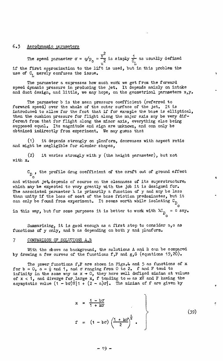
6,3 Aerodynamic parameters
V2 The speed parameter d = q/p0 = - is simply u*
6 as usually defined L
if the first approximation to the lift is used, but in this problem the use of C L merely confuses the issue,
The parameter a expresses how much work we get from the forward speed dynamio pressure in producing the jet. It depends mainly on intake and duot design, and little, we may hope, on the geometrical parameters x,y,
The parameter b is the mean pressure coefficient (referred to forward speed) over the whole of the outer surface of the jet. It is introduoed to allow for the faot that if for exaaple the base is elliptical, then the oushion pressure for flight along the major axis may be very dif- ferent from that for flight along the minor axis, everything else being supposed equal. Its magnitude and sign are unknown, and can only be obtained indireutly from experiment. We may guess that
(1) it depends strongly on planform, decreases with aspect ratio and might be negligible for slender shapes,
(2) it varies strongly with y (the height parameter), but not with x.
the profile drag coeffiaient of the craft out of ground effeot
and without jet,depends of course on the oleanness of its superstructure, which may be expected to vary greatly with the job it is designed for. The associated parameter h is primarily a function of y and may be less than unity if the loss of most of the base friction predominates, but it oan only be found from experiment. It seems worth while isolating CD
0 in this way, but for some purposes it is better to work with XCD = C say,
0
Summarising, it is good enough as a first step to consider a,c as functions of y only, and b as depending on both y and planform.
7 COMPARISON OF SOLUTIONS A.B
With the above as background, the solutions A and B can be compared by drawing a few ourves of the functions f,F and g,G (equations 19,20).
The power functions f,F are shown in Figs.4 and 5 as functions of x for b =0, a=$andl, and CT ranging from 0 to 2, f and F tend to infinity in the same way as x + 0, they have well defiped minima a.t values of x < 1, and diverge for,large x, f tending to 00 as x2 and F having the asymptotic value (1 - bc)-ill + (2 - a)cr]. The minima of f are given by
x = 1 - ba I + kc
f =
(39)
- 19 -

The momentum drag fun&ions g,G are shown in Pig.6 for b = 0: They tend to 0 as x -t 0 in the same way, but g tends to 00 as xZ and G has the asymptotic value 2[cr(l - bo)]n.
In these diagr,ams, whioh cover the practioal range of x, CT and a, the difference between the two solutions is usually much less than I@. For this reason the more tractable solution A will be used henoeforward. The influence of b in the range 50.2 on the funotions f and g is shown in Pigs.? and 8, It may reach 2%.
8 OFTIIvIAOF P/WV
The minima of P/XV as a funotion of a,x can be found as follows, assuming that a,b,o are funotions of y only, and that (bcr)2 can be neglected, i.e. p, << p,.
We then have
PC a WV CT* fy + ou
where 23/2 u+f = 3 x +
The stationary conditions
,i?ll&&Q. = i3liBQ = 0 aG ax
reduce respectively to
(1 - ko)x + 1 + 4 bc(l - kax) = 25'2 63/2 x' ; (4-i 1
(I +ko')x-1+(3-kox) = 0. (42)
P The minima of E, and the values of CT and x at which they occur, are given
by (401, (41>, (42), as funotions of a,b,c and y.
When b = 0 the equations take the comparatively simple form:-
*The curves are drawn up to x = 2 for the sake of comparison, but the A curves oease to be signific‘ant at x = I.
- 20 -

and so
and
4 23 x 0
c2 - E 0 y (1 -5 x)3 = 0
(1 + ko)x = 1
It should be noted from (43) to (45) that as ' -* 0, Y
x+0 like
o-+00 like
ksx+l
CT240 like Y
(43)
w-) z
(4.5) c
The solution is plotted against o/y for a = 0 Cand a = 1 in Fig.9.
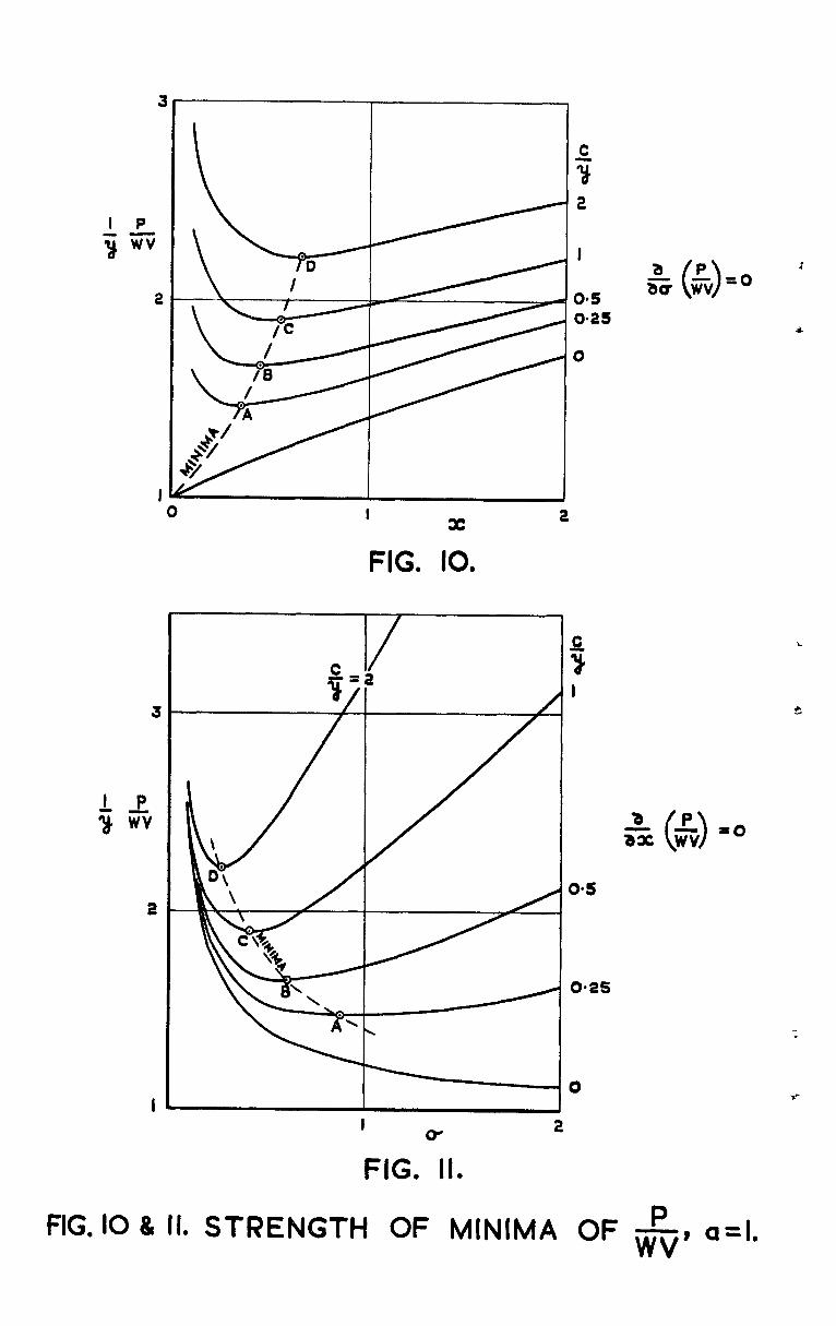
The strength of the minima in x and d are shown respectively in Figs.10 and II, by curves of
(4 L p - ag&nst x under the condition $o y WV = 0.
b) LX Y WV
against CT under the condition -& 5 0
= 0.
The troughs :are sh,aUow between c/y = 0.25 and 1.0, but the x strength becomes large when o/y is small and the o strength large when C/y is large.
It is useful also to know the values cf the jet velocity G and the mass flow m at the power minima.
- 21 -

Forb = 0 these are given by
x U = (2x)4
c
and 1E Y w
= (2x);
and are plotted in Figs.12 and 13.
IP '1 P FinsJ.ly - - = 8 cly z is shown in Fig.14. Y wu
8.1 The effeot of b
A rough approximation to a,x from the general equations (41) and (42) cCan be obtained by treating the terms in b as small quantities of the first order which produoe inorements 6cr, 6x in the solution for b = 0,
We then have from (41) and (42)
sic1 - ka)xj - 2 512 ; lj($i2 x.'12) + $ bc(l - kox) = 0
(47)
6{(1 + ka)x] +++kcsx) = 0 j
where C,X satisfying (43) and (44) are to be used after differentiation.
This oCa3culation yields the following values for a = 1
0.25 -0*41 -1.37
0.5 -0.34 -0.98
1 -0.27 -0.71
2 -0.22 -0.52 ,
the inorements 6cbeing small throughout.
These results are plotted in Fig.15.
The c&Lculstion clearly breaks down for small values of c/y.
- 22 -

9 FURTHER ANALYSIS OF FOWER REQUIRED
Having studied the tot&l power required, we oan now go on to dissect it. The simple hoveroraft analysed here must have two jets*, the annular one providing the power FJ to produce the lift and another
straight one producing:-
PM to overcome the momentum drag
PD to overcome the profile drag.
But as we have seen the forward speed modifies PJ required for hovering by produoing a pressure reoovery aq at the annular jet exit and an addi- tional mean pressure bq over the outer surface of the annular jet which may be either positive or negative. Thus we may write
FJ = I; + PJ 0 cr
suffix o denoting hovering cand (r the increment for the forward speed oondition. Eor the total power P we have
P = (PJ + pJ > + CPM + 'D>
0 o-
the first bracket being supplied by the annular and the second by the straight jet,
9.1 Power dissection forgiven design
We first ccalculate these four components for a given design flying at a given height. In this case it is convenient to use the power function P/Wu sinoe u is constant.
Starting from equations (40) we have
1 & = 2’3/2 Y wu
and by separating the various terms it is easy to show that
*In more advanced designs parts of the annular jets can be inclined backward to reduoe the momentum drag, and it may even become possible to arrange the annulus to supply all the power required.
- 23 -

Vhenb = 0
so that
I 'JC+ 'M
Y wu =
(49)
(50)
and this is always positive.
Pig.16 gives some idea of the relative value of the various items of power over the speed range, using as an illustration the vKLues
x = 0.4, a = 0.5, b = 0, 9 = O& . Y
9.2 Optimum power dissecti.
As another illustration we can use the above equations,multiplied by c', to disseot the minimum power values shown in Pig.7. The results are plotted in Pig.15. One feature of these diagrams, which has already been pointed out by Stanton Jones, is the ratio of PJ the power to produce the lift to PD the profile drag power.
- 24 -

It follows from equation (48) that when b = 0
pJ= pD
5 (*&3/* [(I - *a& + x43.
using the optimum conditions of equations (43) and (44)~ this reduoes to
and so
52 pD
= 2 + 4(1 - a)cr
when a = 1
= 2+4a a=0
where Q is given as a funotion of c/y in Pig.9.
Thus at optimum total power parameter, the power for lift is twioe the power for profile drag, when a = 1, as oan be seen from the upper diagram of Fig.17. This can be contrasted with the aeroplane where the optimum occurs when the drag due to lift is equal to the profile drag. When a= 0 the power for lift is much greater than twioe the power for profile drag (lower diagram of Fig.1 7).
In making these points the large power required to counter the momentum drag, which is in fad part of the mechanism for the production of lift, should not be forgotten. The corresponding ratio at the optimum is
These results apply only at b = 0.
IO EXAMPLES OF PERFORMANCE ESTIMATES
10.1 Design for minimum power
To show how this analysis opn be used for rough performnoe Fstimates, consideroa hoveroraft with ‘an elliptic @anform of fineness ratio T cand jet angle 45 , with an angular clearcanoe of 0.11 radixans. It is to be designed for minimum power at a speed of 100 f.s., i.e. q = 11.9.
From Fig.2, .3/d= 0.16 at n = $-, and so from equation (37), y = 0.2.
Also s = g d* and so we have
- 25 -

h 2 = 0.055
t Ti = 0.585~ l
We shall consider a large r,ange of profile drag coefficients, C going from 0.025 t0 0.2. b is negleoted throughout,
Then using the minimum power values of Figs,9, 12 and 13 we have the following tables for a e 1 and a = 0.
1, y = 0.2, v = 100 a=
a = 0, y = 0.2, v = 100
These tables yield the following solution for W = 10,000 (see Fig.18).
Ct.= 1
Horse Power
Et= 0
- 26 -

Results for any other speed can be got from these tables by noting that
-~
Lx-?- I v2 !
I d,h,t u + j
Iz f
u,G,P,m oc V i
pc a v2 . I 1
Results for a rect,ulgle of the same fineness ratio can be simply deduced by noting from Fig.4 that 43/d at n = &- is praotically the same for rectangle and ellipse, and thus y remains at 0.2. Thus if we assume that rectangle and ellipse have the same profile drag at the same y, the solution is exaotly the same for the rectangle except as regards d,h,t.
If d' is the longer side of the rectangle we have
sinoe the areas are the same, and so
.c d = 0.89.
Thus d,h,t are to be multiplied by this factor to get the rectangle solution.
10.2 Off-design performance -.
Having optimised the design for minimum power at V = 100 we ocon go on to o;iloulate the performance in other conditions, for example
(a) for other speeds n-t the same height,
(b) for other heights at the same speed.
Consider the optimum design for o = 0.1, a = 1 which has been obtained as
w= 10,000, S = 513, d = 36.2, t = 0.52, u = 128.
At v = 100, y = 0.2 we have seen that
x = 0.45, G = 0.61, 5 = 135, h = I-99, m = 14.8, HP = 605.
--27-

L
Some of these quantities mill change in what follows.
(a) mm-n height
In this case x and therefore T and m remCain constant Land we seek the variation of P with CT. This is obtained from the equation
where u = 128, x = 0.45, y = 0,2, k = 2, c = 0.1, W = lO,m.
Thus
where
,P = 19.6 + 12.2~7 e 12.8~ 3/2 W
2 CT=;, 0 The result is shown in Fig.19 where H.P. is plotted against V,
(b) Height variation at the design speed
In this ease o remains constant snd the variation of x and y is such that
xy = 2 = t/4 - oonstant.
Using this relation to transform equation (51) we have
and we have already seen that
The constants in (51) to (53) are
(52)
(53)
(54)
u = 128, k = 2, o- = 0.61, z = 0.45 x 0.2 = 0.09, C = 0.1, w = 10,000.
- 28 -

The equations therefore beoome
E = 3 W 151 y312 + 30.2 y + 6.15
v = a 302 Y
ii? W = 0.00331 f .
The results are plotted in Fig.20 where the Curves have been con- tinued right down to y = 0 although the approximate theory must break downbefore this. The calculation is also questionable because no allowance has been msde for the unknown variation of o with y.
The curves for oases (a),(b) are however useful in giving a rough idea of the power margins that may have to be provided. Expressions for the slo es and (51 P
of the power curves, obtained by differentiating equations (50) , are:-
2-5/2 u c
(1 + lcc)x~ + 3x4 . 3
(55)
i
(56) *
II SECOND APPROXIMATION TO LIFT
The first approximation to lift (equation 23) has been used throughout to simplify the analysis. The seoond approximation can be added in the form of a correction A, using equation (21). For example we have
A & = - & [y sin 0(1 - ba) + 6~3 0
and if b and 6 are neglected, thus including only the vertioal component of the thrust, the correction for typio‘al v‘alues of y and 0 is of the order I@.
12 CRITICAL SPEED? 7
There must be forward speeds at which the actus1 flow ceases to bear any relation to that postulated in this analysis, but the model is so crude that it ocan hardly lead to a criterion, On the assumptions made here the pressure outside the annulus must approach q in the forward parts of the annulus, and so as q rises toward p, (G = 1) we should expeot the curvature of the leading jets to be reversed, Qualitatively there is clear evidence that the front jets ultimately get blown back as the speed rises. The prooess seems to be rather a gradual one than a sudden change to a different regime, but its mechanism is of course much more oomplex than would be
- 29 -

suggested by this approach. When this happens the momentum drag would be relieved, but what happens to the 1st and the profile drag rem2ins obscure, and so as far as m;r information goes it remains an open question whether the power required rises or falls, in relation to that calculated here, as the speed rises. It seems that this doubt can only be settled by onref'ul experiment.
13 THE NEED FOR EXF?ERI~4RNT& CHECKS
The analysis given here is defensible, if at all, only after alignment with experimentn3 results. Indeed it has been prepared mainly as a basis of discussion and use by exprimenters. This could be done in two ways,
(a) The vehicles now being designed usuzlly have features, such as backward inclined main jets and stability jets, that are omitted in this analysis. Thus measurements of their performance could only be plotted on the diagrams suggested here after a good deal of adaptation. On the other hand there is probably much supporting work on simpler models, not yet published, that oould furnish spot checks at various points of this ,anclysis.
(b) Hovercraft performance depends on so many interdependent quanti- ties that basic experiments tend to give w2y in favour of those in support of a particular design. The par,ameters used here are intended to give a clear view of the essentials of the crude flow model on which most onlcula- tions are, I take it, still based, They oan probably be used as the framework for the design of model experiments so chosen as to test the empirioism of current performanoe estimates in the shortest possible time. We should then begin to know where we are.
14 ACKNOWLEDGEMENT
I should like to record the friendly help given me by KS. Igglesden in the preparation of this paper.
-
Geometry
h height 2bove ground
t
6
R
NOTATION
area
perimeter
S/S
maximum dimension
fineness ratio
base
thickness
angle to horizontal, inwards \ * I/ Jet exit
I radius of circle inolined at 0
at jet exit and touohing ground I i

Pressures
Velocities
Parameters
Misoellaneous
PO
PO
H
P
x =
CT =
a
b
C =
=
cDO
k =
L
T
m
D
Dm
DO
P
pO
PJ,'
NOTATION (COPITD1
cushion pressure
mean pressure over outer surface of jet
total head jet at exit
pressure
forward speed, dynamic pressure 4
mean jet velooity at exit
given by p. = $pu2
t R t E,y=pz=xy=z
fraction of q recovered at jet exit
PO/q
profile drag coefficient referred to S
hCD 0
drag coefficient out of ground effects, jet off
2(2 - a) + b G 2(2 - a)
lift
thrust at jet exit
mass flow at jet exit
drag
momentum drag
profile drag
total power required
tot,al power required hovering
'Joy 'my PD parts of P, para.
f,g,j F,G, J 3
p8xn.4
P angular olearrnce = 9 radians
b para* w weight
- 3-l -

LIST OF REFEREZXES
No. Author Title, etc.
1 Stanton Jones, R, Some design problems of hovercraft. IAS Paper Bo.61-45, January 1961.
2 strtmd, T. Invisoid-incompressible-flow theory of statia peripheral jets in proximity to the ground. Jourkl. of Aerospace Soienoes 2 (I), 27-33, January 1961.
3 Chaplin, H, Preliminary study of the hovering performanoe of Stephenson, B, annular jet vehicles in proximity to the ground,
U.S. Navy Dept., Taylor Model Basin. Aero Report 947. P.78137. August 1958.
-
- 32 -
WT.20?8.C.P.608.X3 - Printed in Pnelana

0-i
0 a:
0.1
0
FIG, 1. NOTATION FOR JET,
- - - - RECTANQLE ELLIPSE
O-P 0.4 0.6 0.8 I*0 n
FIG. 20 g/d AGAINST FINENESS RATIO FOR ELLIPSE ANt9 RECTANGLE.
FIG. 3. ARRANGEMENTS PRODUCING THE SAME CUSHION PRESSURE.

----
I 2 X
C
FIG. 4. FUNCTIONS f,F FOR b0, a=[.

3
$9 F
2
I 2 X
FIG. 5. FUNCTIONS f,F FOR 6~0, a=+.

3
&
a-- - - G -
Q= 2*0
FIG. 6. FUNCTION 2,C FOR &=O.

3
2-5
2
f
l-5
I
2
I*5
f
I
I*5
f
I
O-5
0 1 2
X
FIG. 7, EFFECT OF % ON FUNCTION f, a=l.

2
%
I
I X 2
FIG. 80 EFFECT OF 4b ON FUNCTION 9.

O-6
0*4
jC=t 0*2
3
2
I ch
2
FIG. 9. MINIMA OF 6” FOR &=O.
.
I P
ii WV
2
FIG. IO.
2
I
FIG. “II
2
.
2 Y 2
I
o*s 0.2s
0
a P 0
i
bo. Kf=O
i
FIG. 10 & II. STRENGTH OF MINIMA OF &, a=l.

I
0
FlG. 13.
I ch . FIG. 14.
FIG. 12-14. VALUES OF OTHER QUANTITIES AT MINIMUM + l

0=6
096
X
094
o-2
C
3
0 - 2
FIG. 15. EFFECT OF & AT POWER MINIMA,a=l.

O*S w I
X=0*4, Q.-i, e-o, po.4
FIG. 16. ANALYSIS OF POWER REOUIRED FOR GIVEN DESIGN.

2
IL 0 y wv MIN
I
PJo HOVERING
PRESSURE RELIEF
PJ
CL=1
TOTAL PRESSURE RECOVERY
TOTAL
PJ+%Jl
P’ = PJo HOVERING
a=0
NO PRESSURE RECOVERY
I =JY a
FIG. 17, ANALYSIS OF MINIMUM POWER, &=O.

2
800
l4.P
800
400
15
m
IO
I,000
S
500
0
3
A
2
I
0*4
t
0.2
NORSE POWER
CUSHION AREA
HEIGHT -FT.
JET THICKNESS- FT’.
FIG. 18. OPTIMA FOR W = 10,000, V = 100.

1,000
800
600
HP
400
200
0
5, ‘nt CONSTANT
W=10,000, a ‘I, e=o, C=O*I, y 0.2
0 MlNlMlJM POWER AT V =I00
FIG. 19. OFF DESIGN PERFORMANCE, VARIATION WITH SPEED.

600
600
H.P
400
200
0
20
m
IO
w=10,000, a-l, e-o, c-04, V=lOO 0 MINIMA POWER AT ‘#-0*8
0
OESIGN POINT
HORSE POWER
IIj I 4L I A Y 0.3
MASS FLOW
200
JET VELOCITY 100
/ 0 0 0
/ I 2 3 Or’ I &
.
OF;’ 26
I .
FIG, 20. DESIGN P;;FORMANCil VARIATION WITH HEIGHT.

I L.Y.C, C.P. No.&8 533.652.6
A CRUDE THEORY OF HOVERCRt\FT PERFORMANCE AT ZERO TILT. A CRUDE THEORY OF HOVERCRAFT PERFORMANCE AT ZERO TILT. Gates, S.B. November, 1961. Gates, S.B. November, 1961.
The pioneer British hovercraft are Fresumably being designed on a The Pioneer British hovercraft are presumably being designed on a model of the flovr which is naturally a very crude one; little evidence is model of the floiv which is naturally a very crude one; little evidence is available as to the accuracy of the perfOrmaWe estimates that fOllOw from available as to the accuracy of the performance estimates that follow from it; and no critical appraisal of the aerodynamics of the problem at its it; and no critical appraisal of the aerodynamics of the problem at its present level seems to have been published, In this situation the analysis present level seems to have been published. In this situation the analysis given below may serve as a basis of research discussion in three respects? given below may serve as a basis of research discussion in three respects:-
(1) to give a rather clearer view of the assumptions and parameters (1) to give a rather clearer view of the assumptions and parameters involved in the crude theory, involved in the crude theory,
(2) to encourage a stricter comparison between prediction and ad hoc (2) to encourage a stricter comparison between prediction and ad hoc test results as they become available, test results as they become available,
(3) as a point of departure in planning basic experiments that would lead most economically to a better understanding of the matter.
(3) as a Point of departure in planning basic experiments that would lead most economically to a better understanding of the matter.
I-
;..R.C, C.F. No.608 533.,652.6
t’.,R.C. C.P. No.dc8 533.652.6
A CRUDE THEORY OF HOVERCRAFT PERFORMANCE AT ZERO TILT. Gates, SIB. November, 1961.
The pioneer Erftish hovercraft are presumably being designed on a model of the flow which is naturally a very crude one; little evidence is available as to the accuracy of the performance estimates that follow from it; and no critical appraisal of the aerodynamics Of the problem at its present level seems to have been Published. In this situation the analysis given below may serve as a basis of research discussion in three respects:-
(1) to give a rather clearer view of the assumptions and parameters involved in the crude theory,
(2) to encourage a stricter comparison between prediction and ad hoc test results as they become available,
(3) as a point of departure in planning basic experiments that would lead most economically to a better understanding of the matter.

C.P. No. 608
@ Crown Copyright1962
Published by HER MAJESTY’S STATIONERY OFFICE
To be purchased from York House, Kingsway, London w.c.2
423 Oxford Street, London W.1 13~ Castle S&et, Edinburgh 2
109 St. Mary Street, Cardiff 39 King Street, Manchester 2
50 Fairfax Street, Bristol 1 35 Smallbrook, Ringway, Birmingham 5
80 Chichester Street, Belfast 1 or through any bookseller
Printed in England
S.O. CODE No. 23-9013-8
C.P. No. 608