a crossdock consolidation center for local produce: using qgis to

A Crossdock Consolidation Center for Local Produce: Using QGIS to Select an Optimal Site Location

May

2016

James Hollifield, PMP

North Carolina State University

Poole College of Management

Jenkins MBA Program

Report Date: August, 2016

Crossdock Consolidation Centers for fresh produce are a proposed type of

local food distribution infrastructure consisting of loading docks and

coolers for aggregation and storage of product. The Centers are designed

as part of a food distribution network to incentivize large-scale

wholesalers to purchase produce that has been consolidated from rural

and remote farming communities.

The following guide offers a step-by-step example (set in eastern North

Carolina) to determine the optimal location of a proposed consolidation

center so that the procedure can be reconstructed by others. The

example uses the open-source software package QGIS, and utilizes the

location of vacant warehouses as one input. The guide could be useful to

advocates and researchers, as well as economic development personnel

seeking to repurpose underutilized infrastructure.

A companion document provides a facility layout and expected

investment and operating costs: A Crossdock Consolidation Center for

Local Produce: Investment and Operating Cost Estimates (See: ncgrowingtogether.org/Research)

This work was supported by North Carolina Growing Together, a project of the Center for

Environmental Farming Systems, funded by the National Institute of Food and Agriculture, U.S.

Department of Agriculture, under award number 2013-68004-20363. Any opinions, findings,

conclusions, or recommendations expressed in this document are those of the author(s) and do

not necessarily reflect the view of the U.S. Department of Agriculture.

of 37

Table of Contents

Executive Summary ...................................................................................................................................... 2

End State ....................................................................................................................................................... 2

GIS Overview ................................................................................................................................................ 2

Methodology ................................................................................................................................................ 3

Step 1 - Gather, Clean, and Prepare Data .................................................................................................... 3

Roadway Dataset ..................................................................................................................................... 4

Farm Dataset ............................................................................................................................................ 4

Vacant Warehouse Dataset ..................................................................................................................... 6

Step 2 - Prepare QGIS Project ...................................................................................................................... 7

Step 3 - Geocode Data .................................................................................................................................. 9

Step 4 - Import Remaining Data ................................................................................................................ 15

Vacant Warehouse Dataset ................................................................................................................... 15

Roadway Dataset ................................................................................................................................... 18

Step 5 - Import Basemap ............................................................................................................................ 20

Step 6 - Complete Geometric Mean of Farms ........................................................................................... 23

Step 7 - Overlay Desired Buffers ................................................................................................................ 25

Step 8 - Assess Possible Locations and Data ............................................................................................. 27

Create Subset of Warehouses ................................................................................................................ 27

Proximity to Major Road ........................................................................................................................ 29

Proximity to Nearby Wholesaler ........................................................................................................... 32

Step 9 – Repeat Analysis For Possible Farm Clusters ................................................................................ 33

Conclusion and Results .............................................................................................................................. 33

Appendix 1: Connecting to a WMS ............................................................................................................ 35

of 37

Executive Summary The Center for Environmental Farming Systems (CEFS), a partnership between North Carolina State

University, North Carolina A&T University, and the North Carolina Department of Agriculture and

Consumer Services, seeks to “promote just and equitable food and farming systems that…provide

economic opportunities in North Carolina and beyond.”1 To this end, the concept of a “consolidation

center” has been proposed as part of a food distribution network to incentivize large-scale wholesalers

to purchase produce that has been consolidated from rural and remote farming communities.

The following report serves as a procedural framework for managers or researchers who are considering

the viability of this concept as part of their operations and advocacy efforts. Using Geographic

Information Systems (GIS) technology and applicable datasets, this guide offers a step-by-step example

(set in eastern North Carolina) to determine the optimal location of a proposed consolidation center so

that the procedure can be reconstructed by others. The example utilizes the existence and location of

vacant warehouses as one input, and thus could prove useful to economic development officials seeking

to repurpose underutilized infrastructure.

End State The desired end state is to identify the optimal location of a consolidation center based primarily on

minimizing the proximity of the facility to a set of farms within a specific region. Distances from the

optimal location to the nearest major road and nearby cooperating wholesaler facilities are also

measured for consideration. Siting and operational feasibility of the consolidation center (CC) assumes

that the center is used for temporary aggregation of product that has been ordered by one or more

wholesalers. The CC thus has minimal personnel requirements, as it is not a location from which

product is marketed to various buyers; rather, one or more wholesalers communicate directly with a

group of growers which delivers cases of product to the site for pickup.

GIS Overview Geographic Information Systems is a software package that allows the user to visualize data that is

geographically referenced. It can capture, store, analyze, and manipulate these datasets to help the

user better understand the data and, if applicable, develop an optimal solution to their project. Year

after year, GIS software packages become simpler and more user friendly, allowing professionals who

may be unfamiliar with the technology to take advantage of its benefits. In addition, county and state-

level governments often employ or have access to GIS professionals that can assist with a variety of

projects.

This work instruction uses an open source GIS software package called “QGIS”. Open source software

packages are generally free or very inexpensive. However, it should be noted that open source software

can be updated frequently, so it is likely that over time readers of this work instruction will experience

slight differences between what this report demonstrates and the software’s current version. Should

that be the case, the development group of QGIS offers a comprehensive support site at www.qgis.org

where common questions are explained and answered.

1 http://www.cefs.ncsu.edu

http://www.qgis.org/

of 37

Throughout this work instruction, the reader will also be provided with an overview of general GIS

concepts and tips, designated by an asterisk (*) in front of the explanatory paragraph. A general

understanding of these concepts and tips is critical to reproduce the intended results.

Methodology The methodology followed for this work instruction is outlined in Figure 1 below:

Figure 1: Overview of GIS Methodology

Before beginning, QGIS must be downloaded to your workstation. It can be downloaded, for free, at

http://www.qgis.org/en/site/forusers/download.html. Download the version under “Latest release”

and install the program.

Step 1 - Gather, Clean, and Prepare Data A critical and early step in any GIS project is to research, identify, and aggregate any relevant datasets

needed to reach the desired end state. For this particular project, you will need three datasets:

A roadway dataset from local or state government encompassing the geographical area of

consideration

A dataset of all relevant farms in the geographical area of consideration

A dataset of vacant warehouses within the geographical area of consideration that meet the

project’s operational constraints for the consolidation center (square footage, etc)

It is likely that once the data is collected, depending on the format, it will need to be filtered or

categorized to meet the specifications of the project.

*Data Types

GIS readable data comes in a variety of different forms. In general, files are GIS readable if they contain

an attribute that allows data points to be referenced geographically, such as latitude/longitude

coordinates. File types can be distinguished by the extension at the end of the file name (“.doc” at the

Gather, Clean, & Prepare Data

Prepare QGIS Project

Geocode Data Import

Remaining Data

Import Base Map

Complete Geometric

Mean of Farms

Overlay Desired Buffers

Assess Possible Locations &

Data

Repeat Analysis For Possible

Farm Clusters

http://www.qgis.org/en/site/forusers/download.html

of 37

end of a Microsoft Word file, for example). While GIS programs have a large extent of file types they can

import, some of the more common file types have the following file extensions: .shp, .xml, .kml, .kmz,

.txt, .map.

One important distinction between GIS readable file types is “raster” file types and “vector” file types.

Raster files are simply a geographically referenced picture. A user cannot modify or interact with the

file, thus, raster files oftentimes provide very little functionality. Vector files, on the other hand, contain

one or more layers that can be modified and quantitatively analyzed, so the user can interface with the

data to gain additional insight.

One of the most common and universally accepted forms of vector data is what is known as a

“shapefile” (file extension .shp), which is actually a large grouping of individual file types. Because of

this, as data is collected, it is important to keep the data well organized in folders and clearly labeled.

When shapefiles are downloaded they will generally include the entire group of files. To import a

shapefile into a GIS program, the user selects the individual file with the .shp file extension. The

projected .shp file will reference the other files in the group “behind the scenes” to maintain

geographical reference and other data in the GIS program. In addition to shapefiles, it is likely that in

this project the user will work with Microsoft Excel spreadsheets containing geographical references

(latitude/longitude or street addresses, for example).

Data can also come in the form of a Web Mapping Service (WMS). While no WMS was used in this

example, it is recommended that you search for an applicable WMS in your geographical area as these

services can be very helpful and simplify the process. A WMS is a live stream of data provided by an

organization or agency that can be accessed through QGIS. Once connected to a WMS, the connection

provides the same data of an individual dataset but is likely more up-to-date and therefore, more

accurate. This is important for data that is frequently updated; for example, the existence and location

of underutilized infrastructure, such as vacant warehouses. See Appendix A for a step-by-step

procedure of how to connect to a WMS in QGIS.

Roadway Dataset In this example, a roadway dataset shapefile was obtained from an internet search2. This

dataset contains interstates, highways, primary, and secondary roads. Download the file labeled

“North Carolina Highway Shapefile” from the website listed in the reference list at the end of

this report, unzip the group of files, and move them to a folder of your choosing.

Farm Dataset The dataset used for this example, consisting of farm locations, was provided by CEFS for the

purposes of this project. Similar datasets for future projects may be obtained from local

advocacy groups, research groups, or the state government’s Department of Agriculture or

Commerce.

This farm dataset does not need to be filtered; however, as previously noted, datasets in this

form may need to be filtered based on the parameters of your specific project. For instance,

you may want to delete any farm in a certain zip code or county. If any filtering needs to take

place, you have the option of doing this now in the spreadsheet or later in QGIS, but it may be

2 http://www.mapcruzin.com/free-united-states-shapefiles/free-north-carolina-arcgis-maps-shapefiles.htm

of 37

easier to do it now from the spreadsheet. It is important to review the data after it is filtered

to ensure all geographic reference data points are accurate. Small errors in the file such as

incorrect street addresses can result in an incomplete or inaccurate import into QGIS.

Note that this dataset is in the form of a Microsoft Excel spreadsheet. If your project uses

similar spreadsheets, it must contain either 1) an address, city, state, and country for each

farm or 2) a coordinate system such as latitude/longitude for each farm.

The dataset needs to be saved in the comma separated values format (.CSV file extension) for

QGIS to read it. To do this, open the file “Farmer_List” that you downloaded from the CEFS

website. Click “File” –> “Save As” –> “Browse” and in the dialogue window that opens up, click

the dropdown menu “Save as type” and choose “CSV (Comma delimited)”. Navigate to the

folder you wish to save the file to, then click “Save”. In this example, we named the new CSV

file the same as the original file, “Farmer_List”.

Click “Yes” in the dialogue window that opens up.

of 37

For spreadsheets that contain geographical references in the form of street addresses, it is

important that each required criterion (address, city, state, and country) be in a separate

column WITH A COLUMN HEADER once the file is saved as a CSV. After converting the file to a

CSV format, reopen the CSV file to ensure this is the case. If all required criterion is not

included, it can be manually added to the spreadsheet.

Because this spreadsheet does not include state or country columns, those columns will need to

be added manually before or after the file is converted to a CSV.

Vacant Warehouse Dataset This dataset was provided by the North Carolina Department of Commerce and contains all

vacant warehouses in North Carolina. For the purposes of this example, we will not filter any of

the data in this file. However, for future projects, similar datasets will likely need to be filtered

based on the needs of the consolidation center such as square footage, utilities available,

geographic location, etc. Filtering at this stage removes buildings that are unsuitable for

conversion into a Consolidation Center. Notice that for each building in the example Excel

spreadsheet, the sheet contains a street address as well as geographic latitude/longitude

Addresses

redacted for privacy

Addresses

redacted

for privacy

of 37

coordinates. We will import this data using the geographic coordinates to show you how to

import data using both street addresses and coordinate systems as a geographical reference.

This file will also need to be saved in the CSV file format similar to the farm dataset in order for

QGIS to import it. For details on how to save this file as a CSV, please review the instructions

under “Farm Dataset” in this step.

Step 2 - Prepare QGIS Project *Datums and Coordinate Systems

There are numerous coordinate systems that are used to geographically reference the locations of

datasets around the world. Some common examples are latitude/longitude coordinates or state plane

coordinates. In a GIS program, after each data layer is imported, the proper coordinate system must be

selected to properly display the data. From this point forward, selecting the proper coordinate system

for each data layer in QGIS will be of the utmost importance. If all data does not share the same

coordinate system, data layers will be out of alignment or may not appear at all, and distance

measurements may also be inaccurate. A datum is a reference point from which spatial measurements

are made. Datums provide a reference for the program to properly project data in the selected

coordinate system. The most common datums in North America are NAD27, NAD83, and WGS84. In the

context of a GIS program, datums come preloaded into the program and are assigned to each data layer

by the user. Regardless of what coordinate system the data uses, after it is imported it must be saved

as a new shapefile and assigned the same datum as the rest of your map. This is akin to importing the

same dataset again, only now with the correct datum assigned to it. Misaligning reference datums is

one of the most common mistakes in GIS3,4. How to properly perform this action will be discussed as

each data layer is imported.

3 http://wiki.gis.com/wiki/index.php/Datum_(geodesy)

4 http://gis.stackexchange.com/questions/664/whats-the-difference-between-a-projection-and-a-datum

of 37

Before adding any datasets, ensure the proper datum is set for your project. For this project we will be

using the “NAD_1983_StatePlane_North_Carolina_FIPS_3200_Feet” datum. This datum is appropriate

for this example in the state of North Carolina to get accurate distance measurements. It is

recommended that you consult local government GIS analysts to identify the most appropriate datum

for your area, but attempting your project with the more common datums listed above, such as WGS84,

would be a good starting point.

a. From the main screen click “Project” –> “Project Properties”.

b. In the dialogue box that appears, click on the “CRS” tab. Check the box beside “Enable ‘on

the fly’ CRS transformation”. Then beside “Filter” start typing

“NAD_1983_StatePlane_North_Carolina_FIPS_3200_Feet” until you see the datum appear

on the results list. From this list select

“NAD_1983_StatePlane_North_Carolina_FIPS_3200_Feet” (EPSG:102719). Then click “OK”

to save changes.

of 37

Step 3 - Geocode Data Data layers that are geographically referenced using street addresses must be “geocoded” in order for

QGIS to import the data. A plugin has been developed for QGIS that allows geocoding; that is, it allows

the program to convert street addresses to a geographical reference that can be displayed in the

program. For this project, we have one dataset that requires geocoding, the farm dataset. We must

first install the plugin, which is called MMQGIS.

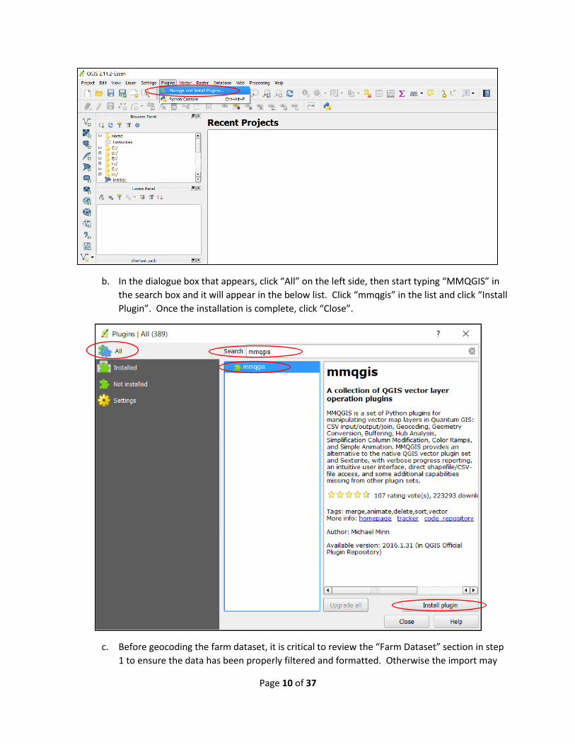
a. From the main screen, click “Plugins” –> “Manage and Install Plugins”.

of 37

b. In the dialogue box that appears, click “All” on the left side, then start typing “MMQGIS” in

the search box and it will appear in the below list. Click “mmqgis” in the list and click “Install

Plugin”. Once the installation is complete, click “Close”.

c. Before geocoding the farm dataset, it is critical to review the “Farm Dataset” section in step

1 to ensure the data has been properly filtered and formatted. Otherwise the import may

of 37

not work. On the main screen, click “MMQGIS” –> “Geocode” –> “Geocode CSV with

Google / OpenStreetMap”

d. In the dialogue box that opens, click “Browse” and navigate to the CSV file that you created

in “Farm Dataset” section of step 1 (named “Farmer_List in this example) and open it.

Ensure that each column header in the CSV file is matched with the appropriate field in the

dialogue box (for example, “Address Field” should match with “Mailing Address”, and so

on). Your dialogue box should look the same as the below screenshot.

As a reminder, if you didn’t add state (NC) and country (USA) columns to the CSV file that

you created, those will need to be added before this step can be completed. You can add

these columns manually into the CSV file that you created.

Click “Browse” beside “Output Shapefile” and “Not Found Output List” and navigate to the

location where you want the output data stored. Be sure to name the files and click “Save”.

In this example we named the output shapefile “Farmer_List”. The output shapefile is the

data that will be displayed on your map and the “not found list” is a populated list of entries

that had incomplete or inaccurate data and could therefore not be geocoded. When you

have decided where to save these files and what label name to give them, click “OK”.

of 37

e. Once the geocoding is complete, you should see a set of data points on your map

representing the locations of the imported farms. A blue bar will temporarily be displayed

at the top of the map to indicate the geocoding was successful. If geocoding failed, the bar

will be red and indicate the geocoding was unsuccessful. The dataset will also show up on

the left side of the main screen under the “Layers Panel”. If any data points could not be

mapped for any reason, they will show up in the “Not Found Output List” document in the

location that you saved it.

*Correcting Projection Misalignments

MMQGIS uses Google geocoding software, and as a result, imports geocoded data using a WGS84

projection. In order for this data to be aligned with the remainder of the project as you continue to

import more datasets, this will need to be corrected. This is also the case with any datasets that are

of 37

imported using latitude/longitude coordinates, so their projections will also have to be modified from

WGS84. It is important to have an understanding of what projection datasets are originally meant for

so that an accurate re-projection can be developed. A good starting point is to know that any data

imported through MMQGIS or with latitude/longitude coordinates has an original projection of

WGS84.

f. Because this dataset was originally imported in the WGS84 projection, a new copy of the

data will have to be created under the projection of our project. To do this, right click on

the layer “Farmer_List.shp” in the “Layers Panel” on the left side of the main screen and

click “Save As…”

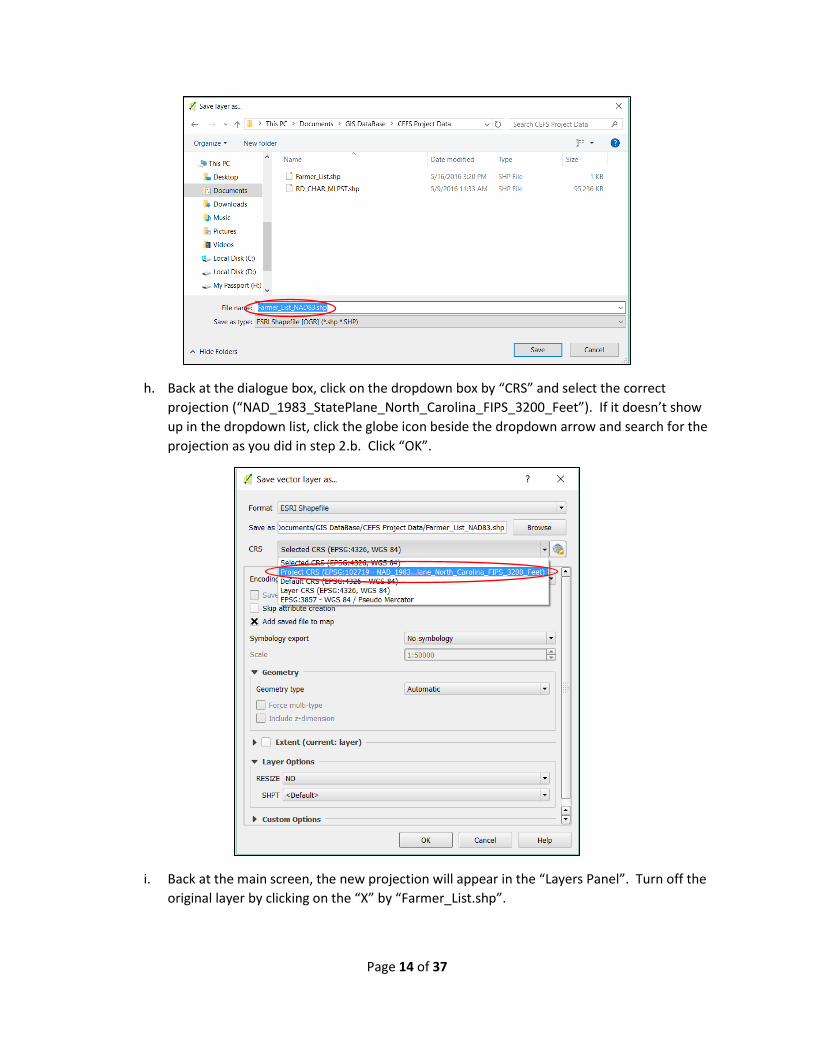
g. In the dialogue box that opens, click on “Browse” and navigate to where you want to save

the new shapefile. To keep your files organized, it is recommended that you label the new

file in such a way that it is easily distinguished as the shapefile with the correct projection.

In this example, we included “NAD83” at the end of the new file name. Click “Save” when

you’ve chosen where to save the file and what to name it.

of 37

h. Back at the dialogue box, click on the dropdown box by “CRS” and select the correct

projection (“NAD_1983_StatePlane_North_Carolina_FIPS_3200_Feet”). If it doesn’t show

up in the dropdown list, click the globe icon beside the dropdown arrow and search for the

projection as you did in step 2.b. Click “OK”.

i. Back at the main screen, the new projection will appear in the “Layers Panel”. Turn off the

original layer by clicking on the “X” by “Farmer_List.shp”.

of 37

Note: This section heavily references a pre-developed online tutorial5. For more information, visit the

website listed in the footnote.

Step 4 - Import Remaining Data Now the remaining two datasets must be imported (roadways and vacant warehouses).

Vacant Warehouse Dataset Recall that we converted this file to a CSV in step 1. As a reminder, any datasets in the form of

Microsoft Excel files should be converted to a CSV format in order to be imported into QGIS.

a. To begin importing this file, select the “Add Delimited Text Layer” icon on the left side of the

main screen (shaped like a comma).

b. In the dialogue box that opens, click “Browse”, navigate to and select the CSV file you

created from the “AccessNC_Vacant_Buildings” Excel file (the CSV file and the Excel file have

the same name in this example). Then click “Open”. The fields in the CSV file should

populate in the dialogue box’s preview screen automatically. Check that the CSV “File

format” is selected. Ensure that the “X field” and “Y field” dropdown menus match up with

the latitude and longitude columns in the spreadsheet. Change the desired name of the

layer if needed and click “OK”.

5 http://blog.mangomap.com/post/74368997570/how-to-make-a-web-map-from-a-list-of-addresses-in

of 37

c. At this point another dialogue box will open to select the correct projection of the data. As

mentioned earlier, the original projection of this dataset is WGS84. In QGIS this projection is

labeled “WGS 84” (EPSG: 4326). You must select this projection (even though it is not the

projection we have been working with in our project) so QGIS can accurately import the

data. Once it is successfully imported we can re-project the data layer in the appropriate

projection. Start typing the EPSG number (4326) in the “Filter” text box until the projection

is displayed in the results. Select the correct projection and click “OK”.

of 37

d. Now that the data layer has been successfully imported, the projection needs to be

modified to align with our project’s projection. Follow the instructions starting at step 3.f

again to save another copy of this data layer in the

“NAD_1983_StatePlane_North_Carolina_FIPS_3200_Feet” projection. In our example we

named the new data layer “AccessNC_Vacant_Buildings_NAD83”. Your screen should now

look similar to the below screenshot with both original data layers unselected and the new

data layers in the correct projections selected.

*“Zoom to Layer”: A useful tool you can use to see the full extent of a dataset is called “Zoom to Layer”.

If the full extent of the dataset is not displayed but it was successfully imported, you can right click on

the dataset in the “Layers Panel” and click “Zoom to Layer”. This will zoom the display out until all the

points in the dataset are visible.

“Zoom to Layer” can also be a valuable tool in discovering errors in the dataset. As it can be seen in the

below screenshot, there are a few errors in the data. For the purposes of this example these errors can

be ignored but for future projects it may be necessary to go back and make corrections. GIS programs

can help you easily identify these errors to avoid hours of manual review.

of 37

*“Identify Features”: In order to quickly identify which data points have errors, you can use the identify

features tool. Select the layer you wish to search on the “Layers Panel”, then select the identify features

tool from the main screen (highlighted in the below screenshot). Click on the data point of interest and

a panel will appear on the right side of the screen with all the information on that data point.

Roadway Dataset Since this dataset is in the form of a shapefile, it will be imported differently.

a. To import shapefiles, click on the “Add Vector Layer” icon on the left side of the main

screen.

of 37

b. In the dialogue box that appears, click “Browse”, then navigate to the folder where you

unzipped the downloaded shapefile in step 1. Select the larger file with the .shp file

extension and click “Open” on both dialogue boxes.

*Layer Order, Color, and Transparency: In the “Layers Panel” on the left side of the main screen, all

your data layers will populate as they are imported. This panel dictates the order in which your data

layers appear from top to bottom. In other words, a data layer may be obscured by another data layer

that is on top of it. To avoid this, you can choose the order in which your data appear by clicking a layer

in the panel and dragging it to the top or bottom. You can also set the transparency of any given layer

by right clicking on the layer in the “Layers Panel” and clicking “Properties” –> “Style” and then sliding

the transparency ruler to the desired level of visibility. In this dialogue box you can also change to color

of a dataset for better contrast and easier viewing.

of 37

c. It is recommended that the roadway dataset be moved towards the bottom of the “Layers

Panel” with the farm and warehouse dataset on top. The roadway dataset is very large so

you may prefer to turn the layer off while moving your map to avoid lags. As a reminder,

you can do this by unchecking the check box beside the data layer in the “Layers Panel”

(highlighted by the red circle in the below screenshot).

Step 5 - Import Basemap *Basemaps: Basemaps serve as a background in GIS software packages. They provide the user with a

geographically referenced map onto which all relevant information is placed. A basemap can provide as

much or as little information as the user wishes.

While there are several ways to import a basemap into QGIS, we will be using a popular plugin called

“OpenLayers” which acts similar to a WMS in that it allows the user to add a number of outside services

to their map:

a. From the main screen, click “Plugins” –> “Manage and Install Plugins”.

of 37

b. In the dialogue box that appears, click “All” on the left hand side then start typing

“OpenLayers” in the search box and it will appear in the below list. Click “OpenLayers

Plugin” in the list and click “Install Plugin”. Once the installation is complete, click “Close”.

Note: OpenLayers may already be installed. If this is the case, it will be indicated by a blue

square beside the plugin name (versus the green puzzle piece seen below) and a check box

beside the blue square. If the plugin is already installed but you get an error when using the

plugin, follow these same steps to uninstall the plugin and reinstall a fresh version.

c. Back at the main menu, click “Web” –> “OpenLayers plugin” –> “Bing Maps” –> “Bing Road”.

of 37

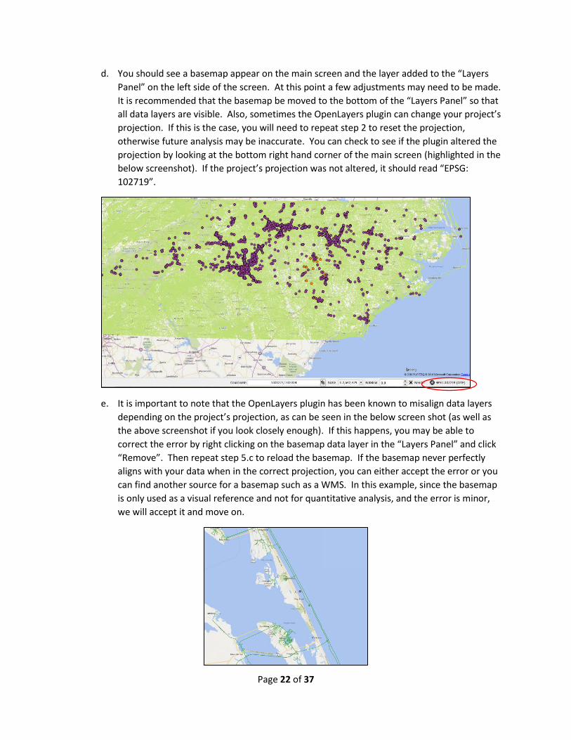
d. You should see a basemap appear on the main screen and the layer added to the “Layers

Panel” on the left side of the screen. At this point a few adjustments may need to be made.

It is recommended that the basemap be moved to the bottom of the “Layers Panel” so that

all data layers are visible. Also, sometimes the OpenLayers plugin can change your project’s

projection. If this is the case, you will need to repeat step 2 to reset the projection,

otherwise future analysis may be inaccurate. You can check to see if the plugin altered the

projection by looking at the bottom right hand corner of the main screen (highlighted in the

below screenshot). If the project’s projection was not altered, it should read “EPSG:

102719”.

e. It is important to note that the OpenLayers plugin has been known to misalign data layers

depending on the project’s projection, as can be seen in the below screen shot (as well as

the above screenshot if you look closely enough). If this happens, you may be able to

correct the error by right clicking on the basemap data layer in the “Layers Panel” and click

“Remove”. Then repeat step 5.c to reload the basemap. If the basemap never perfectly

aligns with your data when in the correct projection, you can either accept the error or you

can find another source for a basemap such as a WMS. In this example, since the basemap

is only used as a visual reference and not for quantitative analysis, and the error is minor,

we will accept it and move on.

of 37

Note: This section heavily references a pre-developed online tutorial6. For more information, visit the

website listed in the footnote.

Step 6 - Complete Geometric Mean of Farms QGIS can determine the central point of a data layer with a tool called “Mean Coordinate(s)”. This tool

finds the location that minimizes the total straight line distance between all the points in a data layer.

Note that this tool may be less accurate for areas with terrain that causes straight line distances to

significantly underestimate actual transportation distances (areas with large mountains or bodies of

water, for example). However, in our area of consideration, this is not the case. QGIS can be configured

to follow roads rather than straight-line distances (using the pgrouting tool), but this requires advanced

SQL coding skills of the user.

a. In the “Layers Panel”, right click the shapefile you created from the farm dataset (called

“Farmer_List_NAD83” in this example) and click “Zoom to Layer”. Then click “Vector” –>

“Analysis Tools” –> “Mean Coordinate(s)”.

b. In the dialogue box that opens, use the dropdown list to select the same file as the “Input

vector layer” (“Farmer_List_NAD83”). Click “Browse”, navigate to where you want to save

the output shapefile, name the shapefile, and click “Save”. In this example we named the

shapefile “Farmer_List_NAD83_Mean”. When finished click “OK”.

6 http://maps.cga.harvard.edu/qgis/wkshop/basemap.php

of 37

c. When complete, you should see the geometric mean appear as a dot in a different color

close to the center of the farm data points.

d. To make this dot appear more visible, you can right click on the data layer in the “Layers

Panel”, and click “Properties”. In the dialogue box that opens, click the “Style” tab on the

left side and change the color, size, or shape of the data point to your liking.

of 37

Step 7 - Overlay Desired Buffers Buffers are used in GIS programs to create a subset of data points that are located in a certain area. In

this example, we are using a buffer to show us which warehouses are close enough to the optimal

consolidation center location and can therefore be considered a viable solution without having to build

a new facility. Buffers are not only good visualizations of radial distances from a central point, but they

are also shapefiles, and can therefore integrate with other data layers for additional analysis (as we will

see later).

On the main screen click on “Vector” –> “Geoprocessing Tools” –> “Buffer(s)”. In the dialogue box that

opens, select the mean coordinate shapefile that you created in the previous step as the “Input vector

layer”. In this example we named it “Farmer_List_NAD83_Mean”. Enter the “Buffer distance” that you

desire. This number will be based on the projection that you use in your project. In our projection we

are using feet as our benchmark measurement so for the buffer we will enter in 52,800 feet (which

of 37

equates to 10 miles). A 10-mile radius is what we have determined as our constraint, your criteria may

be different. Lastly, click, “Browse”, navigate to the location you wish to save the shapefile to and name

the file. In this example we named the file “Farmer_List_NAD83_Mean_Buffer”. Click “Save” then “OK”

and the buffer should appear. Practically speaking, this buffer provides a visualization of what

warehouses are within an acceptable distance from the optimal location of the consolidation center (the

geometric center calculated in step 6).

*Measure Tool: With all the changes to data layer projections, it is a good idea to double check the

distances that you specify in the buffer. Another useful tool in QGIS is the Measure Line, which allows

you to take linear measurements (you can also use the tool to measure areas and angles). To use this

tool, click on the Measure Tool icon on the main screen, specify the units you wish to measure in the

dialogue box, left click on a location to start your measurement, and right click on the ending location to

take the measurement. You can see that our buffer is measuring a 10-mile radius as we intended.

of 37

Step 8 - Assess Possible Locations and Data Let’s recap. At this point you’ve loaded all the data so you can visualize where all the farms and vacant

warehouses are. With the basemap you loaded, it is easy to see roughly where each data point is

actually located. Using the geometric mean of the farms, you’ve also calculated the optimal location for

a consolidation center that minimizes the total linear distance from all farms. Finally, you’ve created a

buffer with a 10-mile radius around the optimal location to better visualize potential vacant warehouses

that meet the criteria of the consolidation center.

Create Subset of Warehouses In this example, we have decided to consider not only the proximity of a vacant warehouse to

the optimal consolidation center location, but also the distance of each potential site to a major

road and to a nearby wholesaler. To do this, we first want to create a separate data layer

containing only the vacant warehouses within the buffer we specified. We will use another

QGIS tool called “Spatial Query” to accomplish this.

a. Right click on the buffer you just created and click “Zoom to Layer”. In the main screen, click

“Vector” –> “Spatial Query” –> “Spatial Query”.

b. In the dialogue box that opens, select the vacant warehouse dataset in the proper

projection under “Select source features from”. In this example we named the dataset

“AccessNC_Vacant_Buildings_NAD83”. Select “Intersects” under “Where the feature” and

select the buffer layer under “Reference features of”. Then click “Apply”.

of 37

c. The dialogue box that appears will list all the vacant warehouses that are inside the buffer.

Click on the icon in the “Selected features” section in the lower left corner and a new data

layer will appear in the “Layers Panel” that only includes the warehouses in this subset.

Then click “Close”.

d. Right click on the new data layer in the “Layers Panel” and click “Open Attribute Table”. You

can use the table to review all the attributes of the warehouse subset within your buffer. All

of the attributes that were included in the original spreadsheet are also included in this

subset.

of 37

In this example, this step may seem unnecessary because there are only 3 vacant

warehouses in the 10-mile buffer, but this tool can be quite useful and save you a lot of time

if you find that you have several data points within the chosen buffer and need to assess

each one.

e. In the “Layers Panel” turn on this new data layer and deselect the original vacant warehouse

dataset. We are now only concerned with the warehouses that are captured in our buffer.

Now that we’ve created the separate data layer, we can assess the proximity of each warehouse to a

major road and a nearby wholesaler.

Proximity to Major Road To determine the proximity of each warehouse to a major road we can use another QGIS tool

called “Shortest path”, which uses the roadway shapefile to determine the shortest driving

distance from one point to another.

a. First, you must choose the settings for the tool. On the main screen, click “Vector” –> “Road

graph” –> “Settings”.

of 37

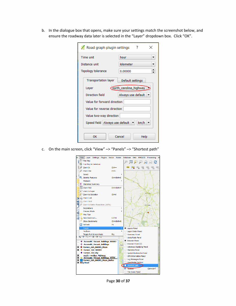
b. In the dialogue box that opens, make sure your settings match the screenshot below, and

ensure the roadway data later is selected in the “Layer” dropdown box. Click “OK”.

c. On the main screen, click “View” –> “Panels” –> “Shortest path”

of 37

d. This will pull up a new panel on the left side of the main screen.

e. Zoom in to the area you want to analyze (here we focus on the upper half of the buffer),

click on the cross beside the text box under “Start” and then click on the starting location on

the map (in this example the starting location will be one of our vacant warehouses within

our buffer). Next, click on the cross beside the text box under “Stop” and then click on the

closest major road. Then click “Calculate” in the panel. The calculation may take a couple of

minutes.

Note: In this example we’ve selected what roads we consider “major”. However, individual

projects may have different criteria for a road to be considered “major”.

f. When the calculation is complete, a red line will be highlighted from your start and stop

locations and the total distance will be displayed in the “Shortest path” panel. You can redo

the calculation with a new stop location based on the closest exit from a major road to get a

more accurate distance if you wish. This additional distance is circled in the below

screenshot.

of 37

Note: This tool only calculates distances in kilometers so you will have to make any

conversions manually.

Proximity to Nearby Wholesaler Now we must select a nearby wholesaler of interest and use the same tool to determine the

driving distance to that wholesaler. The easiest way to do this is to look up the address online

and use an online reference like Google Maps to identify the location of the address. Then

simply make that location your start or stop point in the “Shortest path” panel. In our example,

we use the produce wholesale/distributor FreshPoint, located southwest of the Raleigh-Durham

International Airport. Calculating the shortest path between two locations that are farther away

may take additional computing time.

Repeat this analysis for every warehouse inside the 10-mile buffer (finding the proximity to the nearest

major road and a nearby wholesaler). Using this information, we can now make a quantitatively-backed

analysis to identify the optimal warehouse to choose as our consolidation center.

It is important to reiterate that in this project we have chosen three criteria to select our optimal

consolidation center location:

of 37

Minimizing the proximity to the largest number of farms

Minimizing the proximity to a major road

Minimizing the proximity to a nearby wholesaler of interest

However, for your project there may be a variety of other constraints and criteria that must be met or

weighted differently in order for your location to be considered “optimal”. These include criteria such

as the farthest distance between farmers or the proximity of an individual, larger farm to the optimal

location. The goal of this instruction is to provide you with an understanding of the QGIS program and

some of the program’s tools so that you can leverage this technology to meet your individual project

needs.

Step 9 – Repeat Analysis For Possible Farm Clusters It is possible that your data will have obvious clusters of farms, say for instance in an eastern and

western region. If this is the case, it is recommended that you separate the data into two or more

regions while the data is still in an Excel format (before it is imported into QGIS). To do this, you can

separate and filter the data by any geographical attribute such as latitude/longitude coordinates or

counties. Then repeat this analysis for each region.

Conclusion and Results In this example we assessed 1 of the 3 warehouses within the 10-mile buffer that potentially satisfies

our criteria for a consolidation center. Using the identify features tool described in step 4, you can see

this warehouse is located at 220 Olive Farm Drive, Sanford, NC. We compiled the below statistics using

some of the previously described tools to further analyze the optimal site (the geometric mean of the

farms calculated in step 6) as well as the location of this warehouse. Short descriptions on how to

obtain some of these statistics are described below the table:

Optimal Site Location (Geometric Mean of Farms)

35.249° N, 079.171° W

% of Farms Within 10 Miles of the Optimal Site

21%


85%


100%

Three Farms Closest to Optimal Site 108 CVP Lane, Cameron, NC

5948 Lemon Springs Road, Sanford, NC 1606 Pickett Road, Sanford, NC

Location of Vacant Warehouse Within 10 Miles of Optimal Site

220 Olive Farm Drive, Sanford, NC

Distance from Vacant Warehouse to Nearest Major Road

10.7 miles

Distance from Vacant Warehouse to Interested Wholesaler

47.7 miles

of 37

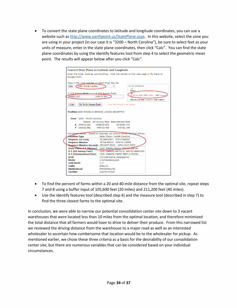
To convert the state plane coordinates to latitude and longitude coordinates, you can use a

website such as http://www.earthpoint.us/StatePlane.aspx. In this website, select the zone you

are using in your project (in our case it is “3200 – North Carolina”), be sure to select feet as your

units of measure, enter in the state plane coordinates, then click “Calc”. You can find the state

plane coordinates by using the identify features tool from step 4 to select the geometric mean

point. The results will appear below after you click “Calc”.

To find the percent of farms within a 20 and 40-mile distance from the optimal site, repeat steps

7 and 8 using a buffer input of 105,600 feet (20 miles) and 211,200 feet (40 miles).

Use the identify features tool (described step 4) and the measure tool (described in step 7) to

find the three closest farms to the optimal site.

In conclusion, we were able to narrow our potential consolidation center site down to 3 vacant

warehouses that were located less than 10 miles from the optimal location, and therefore minimized

the total distance that all farmers would have to drive to deliver their produce. From this narrowed list

we reviewed the driving distance from the warehouse to a major road as well as an interested

wholesaler to ascertain how cumbersome that location would be to the wholesaler for pickup. As

mentioned earlier, we chose these three criteria as a basis for the desirability of our consolidation

center site, but there are numerous variables that can be considered based on your individual

circumstances.

http://www.earthpoint.us/StatePlane.aspx

of 37

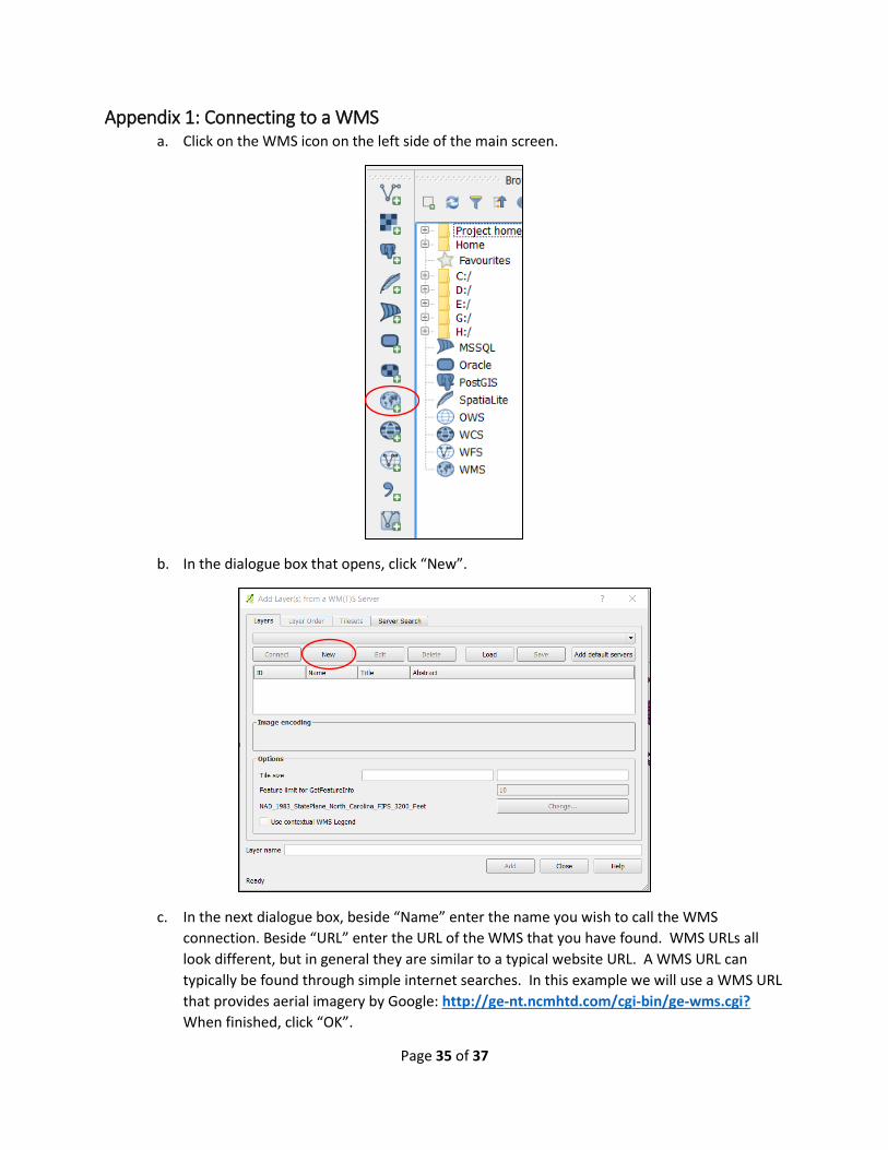
Appendix 1: Connecting to a WMS a. Click on the WMS icon on the left side of the main screen.

b. In the dialogue box that opens, click “New”.

c. In the next dialogue box, beside “Name” enter the name you wish to call the WMS

connection. Beside “URL” enter the URL of the WMS that you have found. WMS URLs all

look different, but in general they are similar to a typical website URL. A WMS URL can

typically be found through simple internet searches. In this example we will use a WMS URL

that provides aerial imagery by Google: http://ge-nt.ncmhtd.com/cgi-bin/ge-wms.cgi?

When finished, click “OK”.

http://ge-nt.ncmhtd.com/cgi-bin/ge-wms.cgi?

of 37

d. Back in the first dialogue box, click “Connect” and you will see the WMS appear. Select one

of the WMS layers and click “Add”.

e. The new imagery will appear on your map and the WMS layers will appear in your “Layers

Panel”.

a crossdock consolidation center for local produce: using qgis to

Documents