a cross-layer methodology for design and optimization of
TRANSCRIPT

A Cross-Layer Methodology forDesign and Optimization of Networks in 2.5D Systems
Ayse Coskun1, Furkan Eris1, Ajay Joshi1, Andrew B. Kahng2,3, Yenai Ma1, and Vaishnav Srinivas2
1ECE Department, Boston University, Boston, MA, USA; 2ECE and 3CSE Departments, UC San Diego, La Jolla, CA, [email protected],[email protected],[email protected],[email protected],[email protected],[email protected]
ABSTRACT2.5D integration technology is gaining popularity in the designof homogeneous and heterogeneous many-core computing sys-tems. 2.5D network design, both inter- and intra-chiplet, impactsoverall system performance as well as its manufacturing cost andthermal feasibility. This paper introduces a cross-layer method-ology for designing networks in 2.5D systems. We optimize thenetwork design and chiplet placement jointly across logical, physi-cal, and circuit layers to achieve an energy-e�cient network, whilemaximizing system performance, minimizing manufacturing cost,and adhering to thermal constraints. In the logical layer, our co-optimization considers eight di�erent network topologies. In thephysical layer, we consider routing, microbump assignment, and mi-crobump pitch constraints to account for the extra costs associatedwith microbump utilization in the inter-chiplet communication. Inthe circuit layer, we consider both passive and active links with �vedi�erent link types, including a gas station link design. Using ourcross-layer methodology results in more accurate determination of(superior) inter-chiplet network and 2.5D system designs comparedto prior methods. Compared to 2D systems, our approach achieves29% better performance with the same manufacturing cost, or 25%lower cost with the same performance.ACM Reference Format:Ayse Coskun1, Furkan Eris1, Ajay Joshi1, Andrew B. Kahng2,3, Yenai Ma1,and Vaishnav Srinivas2. 2018. A Cross-Layer Methodology for Design andOptimization of Networks in 2.5D Systems. In IEEE/ACM INTERNATIONALCONFERENCE ON COMPUTER-AIDED DESIGN (ICCAD ’18), November 5–8, 2018, San Diego, CA, USA. ACM, New York, NY, USA, 8 pages. https://doi.org/10.1145/3240765.32407681 INTRODUCTION
The need to sustain the historical performance and cost scal-ing in computing systems has led to a growing interest in 2.5Dsystems [1, 8, 9, 15, 16, 29]. In 2.5D design, multiple chiplets areplaced on a silicon interposer, and the chiplets communicate usinglinks integrated into the interposer. 2.5D integration technology pro-vides multiple potential bene�ts compared to 2D systems, includinggreater system performance within thermal constraints [12], het-erogeneous integration of multiple technologies [1, 6], and reducedoverall system cost [16]. However, 2.5D integration technology alsoopens up a number of design challenges, ranging from circuit andphysical challenges (design and routing of inter-chiplet links, place-ment and �oorplanning of chiplets on the interposer, microbump
Permission to make digital or hard copies of all or part of this work for personal orclassroom use is granted without fee provided that copies are not made or distributedfor pro�t or commercial advantage and that copies bear this notice and the full citationon the �rst page. Copyrights for components of this work owned by others than ACMmust be honored. Abstracting with credit is permitted. To copy otherwise, or republish,to post on servers or to redistribute to lists, requires prior speci�c permission and/or afee. Request permissions from [email protected] ’18, November 5–8, 2018, San Diego, CA, USA© 2018 Association for Computing Machinery.ACM ISBN 978-1-4503-5950-4/18/11. . . $15.00https://doi.org/10.1145/3240765.3240768
assignment, etc.) to architectural and system-level challenges (de-sign of the inter-chiplet network architecture, partitioning a systeminto 2.5D-integrated heterogeneous functional components, etc.).Many other technical and business challenges, including design forthermomechanical stress, test strategy, and supply chain structure,are identi�ed by Radojcic [26].
In this paper, we perform a cross-layer co-optimization of2.5D inter-chiplet network design and chiplet placement. Our co-optimization methodology focuses on network topologies, linkcircuit options, and microbump pitch- and interconnect RC-awarerouting of links. It maximizes performance and/or minimizes costat the system level, while satisfying system power and thermalconstraints. The need for such a cross-layer methodology as ourscan be easily seen by considering the following. If we adopt a top-down approach, an architecture analysis of network topologiestells us that high-radix, low-diameter networks should be usedfor inter-chiplet networks, as they provide the best overall systemperformance (in instructions per cycle). However, in the physicallayer, realization of high-radix, low-diameter networks requireslong wires, which can limit the network performance and, hence,the overall system performance. Using repeaters on long wires toimprove performance would necessitate active (rather than pas-sive) interposer technology. Since active interposers are 10⇥ moreexpensive than passive interposers [25], the system cost equationchanges and the top-down intuition is �awed. On the other hand, abottom-up, cost-centric perspective prompts the use of a passiveinterposer, which can only support repeaterless links in the circuitlayer, thus limiting link performance and maximum link length.This leads to the adoption of low-radix, high-diameter networks atthe inter-chiplet level, which lowers overall system performance.
Our work �lls a signi�cant gap in the literature on inter-chipletnetwork design and �oorplan/placement optimization of 2.5D sys-tems. No prior work has simultaneously considered thermal be-havior of chiplets, multiple potential network topologies, multipleinter-chiplet link options, and physical design constraints asso-ciated with routing these links. Thus, previous approaches canincorrectly evaluate cost, performance, power and thermal feasibil-ity, as well as other important parameters of 2.5D system solutions.Consequently, there is a risk of identifying suboptimal inter-chipletnetwork and 2.5D system �oorplan solutions, which can lead toine�cient architectural decisions. For example, in our recent work[12], we describe a methodology to place chiplets (connected by amesh) that results in thermally-safe, high-performance, and low-cost 2.5D systems. However, in the logical layer, we only consider aUni�ed-Mesh1 network topology. In the physical layer, there is noaccounting of the area overhead associated with the microbumps
1We classify networks either as Uni�ed when we have single-level logical topologyor as Global-Local when we have two-level logical topology with Global as the inter-chiplet and Local as the intra-chiplet level logical topology. A Uni�ed network logicallytreats all cores as if they are on the same die and we connect them as such, while in aGlobal-Local network we have a hierarchy of connections.

required for the inter-chiplet links. In the circuit layer, we consideronly one type of link. As elaborated below, the present paper showsthat a careful accounting of microbump overhead, along with con-sideration of multiple network topology options and link designoptions, leads to a solution that can achieve 16% higher perfor-mance at comparable cost, and/or 18% lower cost at comparableperformance, with respect to our prior best solutions.
The main contributions of this paper are as follows:• We develop a cross-layer co-optimization methodology thatoptimizes inter-chiplet network design jointly with chipletplacement across logical, physical, and circuit layers. Ourmethodology optimizes a given 2.5D system for performance,cost, and wirelength, while ensuring that it is thermally safe.The outcome of the co-optimization comprises placementof chiplets on the interposer, logical topology of the inter-chiplet network, and circuit design and routing of the linksthat form the network.• Our co-optimization considers a rich solution space. (i) Inthe logical layer, we consider a variety of Global, Local, andUni�ed network topologies. (ii) In the physical layer, weincorporate well-calibrated microbump overhead modelsinto our area and cost models. We further consider the �-nite density of microbumps per unit die area, and assessachievable physical wiring distances (hence, achievable linklatencies). (iii) In the circuit layer, we explore repeaterlessnon-pipelined, repeaterless pipelined, repeatered pipelined,and repeatered non-pipelined types of inter-chiplet links. Wefurther consider a gas station link design to enable pipeliningin passive inter-chiplet links.• Our heuristic-based cross-layer co-optimization has severalnovel elements. (i) For a given chiplet placement and networktopology, we perform routing and microbump assignmentusing a �ow-based mixed integer-linear program (MILP) tominimize the maximum link latency. (ii) We use workload-and network throughput-aware thermal simulation outputsfrom HotSpot [32] to assess the thermal feasibility of place-ment and network topology solutions. (iii) We apply simu-lated annealing to search over our high-dimensional systemsolution space.
2 RELATEDWORKRelated work on design and optimization of networks in 2.5D
systems can be categorized based on the design layer: logical, phys-ical, and circuit. Unlike our present work, previous approaches aregenerally limited in scope to a single layer of design.
In the logical layer, Kannan et al. [16] have evaluated various log-ical topologies for 2.5D systems, but their work does not considermicrobump area overheads, di�erent inter-chiplet link options, orphysical implementation of the 2.5D layout. Ahmed et al. [2] pro-pose a hierarchical mesh network for inter-chiplet communication.Both Kannan et al. [16] and Ahmed et al. [2] assume a “minimally ac-tive” interposer, which could be unrealistic from a cost perspective(see Section 3). Akgun et al. [3] evaluate three specialized memory-to-core network topologies, yet the evaluation is limited to thelogical layer with a static placement of chiplets, and implicationsof design choices on physical and circuit layers are not explored.None of these works take thermal e�ects into account or perform aphysical design optimization of the 2.5D inter-chiplet network.
In the physical layer, Funke et al. [14] have proposed variousalgorithms that exhaustively search for optimal placement androuting solutions for up to six chiplets. The recent work of Os-monolovskyi et al. [24] handles up to 11-chiplet design complexity
SiP Substrate
Flip Chip Bumps
Backside Metal Layer
Frontside Metal Layer
Through Silicon Vias Interposer Substrate
Chiplet #1 Chiplet #2
Microbumps
Figure 1: The cross-section of a 2.5D system.
using pruning methods. Minz et al. [22] and Fang et al. [13] focuson routing of inter-chiplet links on an interposer. Liu et al. [20]aim to reduce the number of metal layers in the interposer. Theseworks do not consider thermal e�ects while �nding placement androuting solutions. In our prior work [12], we propose a thermally-aware chiplet placement solution. However, our prior work doesnot perform routing and only computes a placement solution.
In the circuit layer, research has generally focused on per-linkanalyses and optimizations, without considering overheads or trade-o�s with respect to network or system throughput. The works ofStow et al. [28] and Karim et al. [17] explore both repeaterless andrepeatered electrical links, while Shamim et al. [27] and Grani etal. [15] respectively consider wireless and photonic links. Ehrettet al. [11] analyze the power and delay overhead of microbumpsand conclude that microbump overheads are small. However, theyoverlook electrostatic discharge (ESD) capacitance, which leads tounderestimation network of power and latency.
In contrast to these previous works, our methodology jointlyconsiders logical, physical, and circuit design of the inter-chipletnetwork. We evaluate a variety of logical topologies, while beingaware of the network design feasibility in both the circuit layerand the physical layer. In the circuit layer, we evaluate various linkdesign options. In the physical layer, we develop a thermally-awareplacement and routing solution. Our cross-layer methodology, thus,obtains 2.5D system solutions that, having more complete andaccurate modeling foundations, come closer to de�ning the trueenvelope of 2.5D system performance and cost under power andthermal constraints.
3 INTER-CHIPLET NETWORK DESIGNA cross-layer inter-chiplet network design methodology must
comprehend a vast design space that spans the logical, physicaland circuit design layers. In this section, we describe the designspace for each of these three layers, along with key parameters ofinterest.
3.1 2.5D System ArchitectureOur studies use a 256-core homogeneous (i.e., all cores are of
the same type) system. To enable comparisons against the previousliterature, we speci�cally adopt the core design used in our priorwork [12]. Cores have the following architectural speci�cations:• 16KB I/D L1 Cache• 256KB Private L2 Cache• 0.93mm2 Core + L1 Area• 0.35mm2 L2 Area• 1.28mm2 (1.13mm ⇥ 1.13mm) Total Area [33]• 18mm ⇥ 18mm Total 256-core Chip Area
Each core, together with its L1 and L2 caches, has a square layout.Following our prior work [12], we study chiplet-based integration of16 identical chiplets on an interposer, where each chiplet contains 16cores. Figure 1 illustrates the cross-section view of a 2.5D system.We assume that the 22nm chiplets are placed on an interposer

that is designed in 65nm process technology. Microbumps connectthe chiplets to the interposer substrate. The system is placed ona System-in-Package (SiP) substrate, with C4 (“�ip chip bumps”)connecting the interposer to the SiP substrate. We enable directcomparison of this work with our prior work [12] by designing aUni�ed-Mesh network using our cross-layer methodology. It shouldbe noted that our broader conclusions are agnostic of the speci�ccore count, core architecture, and technology nodes for the chipletsand the interposer.
3.2 Logical LayerIn the logical layer, we explore several di�erent network topolo-
gies [35]. We limit the intra-chiplet network to Local-Mesh andLocal-Cmesh topologies. For the inter-chiplet network, we designand evaluate Global-Butter�y, Global-Butterdonut [16], and Global-Mesh topologies. For the Uni�ed networks, we evaluate Uni�ed-Mesh and Uni�ed-Cmesh.
3.3 Physical LayerPhysical design of the inter-chiplet network consists of place-
ment of the chiplets, along with a routing solution connecting thechiplets2 that is consistent with the chosen network topology (seeSection 3.2). The placement of chiplets a�ects the temperature mapand the length of the links among chiplets, while the routing solu-tion in turn a�ects the microbump assignment and circuit choicesfor the link. Further, we explicitly account for the area overhead ofmicrobumps and the associated inter-chiplet drivers and receiversplaced along peripheral regions of the chiplets.
Inter-chiplet links can be routed on a passive or an active in-terposer. Microbumps and ESD protection are required at the be-ginning and the end of links that go through interposers, and thisdesign constraint adds capacitance [17]. Passive interposers costless due to their lower manufacturing cost and higher yield [25]. Ac-tive interposers allow for repeaters and/or �ip-�ops (for pipelining)on the interposer. This enables better link bandwidth and latency atthe expense of higher manufacturing cost [25]. We conduct a pre-liminary study of the performance bene�t of an active interposer.We observe 2⇥ to 3⇥ latency improvements for the same link lengthand 50% longer links for the same throughput, but this comes at a10⇥ cost overhead ($500 per wafer for passive interposer vs. $5000per wafer for active interposer [25]). Given this cost overhead, werule out active interposers as a realistic option in the near term,and do not consider this option in our present study.
Passive interposers limit the bandwidth of the signal by degrad-ing rise/fall times. Hence, we use a gas station link, where we can“refuel” a passive link using repeaters and/or �ip-�ops that are in-side other chiplets along the way from the source chiplet to the sinkchiplet. Figure 2 shows two implementation schemes for a chiplet-to-chiplet link. Figure 2(a) shows the top view of the paths for thetwo links connecting Chiplet #1 to Chiplet #3, which are far (e.g.,> 10mm) from each other. Figure 2(b) shows a cross-sectional viewof the two paths between Chiplet #1 and Chiplet #3. Path 1 usesChiplet #2 as a gas station, while Path 2 is a direct connection with-out any gas station. It is important to note the di�erences betweenan inter-chiplet repeaterless pipelined link and a gas station link. (i)Pipelining repeaterless links requires an active interposer, while forgas station links we can use a passive interposer. (ii) Active elementsrequired for repeaterless pipelined links are designed using the ac-tive interposer’s technology node, while active elements required
2We aim to minimize the maximum physical link distance, which is our proxy for linklatency.
Chiplet #1
Chiplet #1
Chiplet #2
Chiplet #3
1 2
21
Chiplet #2 Chiplet #3
2 1 21
KeyOn-ChipletChannel
On-InterposerChannel
(a) Top View (b) Cross-Section View
Interposer
Interposer
Figure 2: Possible link implementation schemes includingGas Station, which is shown as Path 1.
Core
CacheCore
Cache
Microbumps h
(a) Chiplet Without Microbump Area
(b) Chiplet With Microbump Area
(c) Chiplet Arrangement
S1
S1
S3
S3
S2
S2
Figure 3: Illustration of the extra microbump area requiredper chiplet.
Uni�ed Uni�ed Global Global Global GlobalMesh Cmesh Mesh Bu�erfly Bu�erdonut Clos
#microbumps 1024 512 256 256 256 2048h (mm) 0.585 0.315 0.18 0.18 0.18 1.125
Chiplet Size (mm) 5.67 5.13 4.86 4.86 4.86 6.75Microbump Area Overhead (%) 58.76 29.96 16.64 16.64 16.64 125.0
Table 1: Microbump area overhead for network topologieswith shielding overhead included.
for gas station links are designed using the chiplet’s technologynode. (iii) Using gas station links requires additional microbumps,and in turn, has an area overhead.
When considering 2.5D inter-chiplet links, recent works haveoverlooked the microbump overhead while assessing 2.5D inte-gration bene�ts. Generally, the number of required microbumpswill change according to the network topology. An increase in thenumber of inter-chiplet links increases the number of required mi-crobumps. Further, additional microbumps (20% according to Rado-jcic [26]) must be reserved for power delivery and signal shieldingpurposes. Figure 3 shows the chiplet without and with the extraarea required for microbumps. Table 1 presents the overhead dueto microbumps for di�erent network topologies designed usingrepeaterless non-pipelined links. The calculations are for the 256-core system divided across 16 chiplets, with each chiplet having anarea of 4.5mm ⇥ 4.5mm, and a microbump pitch of 45um. Here, hindicates the width of the extra space along the chiplet periphery re-quired for the microbumps used for the inter-chiplet links [26]. Theuse of gas station link design will further increase microbump count.We do not list the microbump area overhead associated with use ofgas station links since this depends upon the placement solution aswell as the network type.
3.4 Circuit LayerThere are multiple circuit design options for inter-chiplet links.
For passive interposers, the link on the interposer itself is repeater-less, but with the inclusion of gas stations, the link can use repeatersand/or �ip-�ops (for pipelining) in intermediate chiplets to regener-ate and retime the signal. We limit tr ise/tc�cle to less than 0.5, to en-sure full voltage swing at all nodes in the presence of non-idealitiessuch as supply noise and jitter. We also explore tr ise/tc�cle of 0.8that allows us to go longer distances without repeaters. Relaxingthe clock period or allowing for multi-cycle bit-periods permits usto use longer inter-chiplet links.

Technology Node 22nm 65nmWire Thickness 300nm 1.5µmDielectric Height 300nm 0.9µm [17]Wire Width 200nm 1µm [26]Cbump 4.5f F 4.5f F [17]Cesd 50f F 50f F [17]C�_t (Gate Cap) 1.08f F /µm 1.05f F /µmCd_t (Drain Cap) 1.5 ⇥ Cg 1.5 ⇥ CgRt (Inverter resistance) 450� · µm 170� · µmWire Pitch 0.4µm 2µm [26]Flip-Flop Energy per Bit 14f � /bit [10] 28f � /bit [18]Flip-Flop tc�q + tsetup 49ps [10] 45ps [18]
Table 2: Technology node parameters.
Figure 4: Distributed inter-chiplet link models:(a) repeaterless link and (b) gas station link, in a passive
interposer.Figure 4 shows distributed circuit models for link types; (a) re-
peaterless link in passive interposer, and (b) gas station link inpassive interposer. We model wire parasitics using a distributed,multi-segment � model. We use 22nm technology parameters forintra-chiplet components (drivers, receivers, repeaters, and �ip-�ops of the links), while we use 65nm parameters for the inter-chiplet components of the links. Table 2 shows technology parame-ter values used in our experiments. We calculate capacitance andresistance based on the model in Wong et al. [30], and we calibrateour stage and path delay estimates based on extraction from layoutand Synopsys PrimeTime timing reports.
4 CROSS-LAYER CO-OPTIMIZATIONIn this section, we describe how we optimize the network de-
sign across the layers described in Section 3, using a cross-layerapproach. We show our evaluation framework in Figure 5. We �rstconstruct oracles for system performance, cost, and interconnectperformance. Each of these oracles gives us an element (perfor-mance, cost, and latency) of the co-optimization function. Ourmethod for �nding a placement solution of chiplets uses a sim-ulated annealing algorithm. We build a search and sort engine thatplaces the oracles and the placement algorithm in a loop to searchfor a solution across the logical, physical and circuit layers. Table4 shows the notations we use in the various steps of our cross-layer co-optimization methodology. The placement algorithm usesHotSpot to determine the thermal pro�le and an MILP is used to�nd the optimal routing solution. Thus, we determine the feasi-bility of each placement using HotSpot simulations and the MILPsolution.
4.1 System Performance OracleWe build a system performance oracle that tells us the over-
all system performance and total core power for a given networktopology, voltage-frequency setting, and link latency. To create theoracle, we use Sniper [7] to precompute system performance fora variety of network topologies, voltage-frequency settings, andlink latencies. Our system architecture is the 256-core architecturedescribed in Section 3.1. Eight memory controllers are placed nextto the top and bottom rows of cores. We implement the inter-chipletand intra-chiplet network models discussed in Section 3.2 usingeither passive links or gas station links (see Section 3.3). For passivelinks without gas stations, we vary inter-chiplet latency values from
∀
Interconnect Oracle
System Perf. Oracle
Cost ModelOracle
IPS
S0
S S'
Routing AlgorithmHotSpot
If T(s)< Tth and L(s) < Lth
No
if K<
No
if AP >random(0,1)
Accept Probability =e T(s)-T(s')
KL(s)-L(s')
K
T(s) T(s') L(s) L(s')
Yes No
S' New S*
K decays with each iteration
Latency Constraint
Cost
Oracle Table
Sorted Table
, , Does Not Exist
Does Exist
McPATIPS
∀
(1) Precompute
(2) Sort
(3) Search
Power Trace
Target Latency
Length Interposer Width
Simulated Annealing
Optimal Output
∀(v,f)∀Network
*e
Figure 5: Cross-layer co-optimization flow.
1 to 5 cycles, and for gas station links we consider 2- or 3-stagepipelined links. We apply three voltage-frequency settings, (0.9V,1000MHz), (0.89V, 800MHz) and (0.71V, 533MHz). We fast-forwardsequential initialization regions and simulate up to 10 billion in-structions in the region of interest using Sniper, with all 256 coresactive, to collect performance statistics for �ve benchmarks. Thistakes 1.7k CPU hours. We use McPAT [19] to convert the perfor-mance results to power traces needed for generating the thermalpro�le.
4.2 Cost OracleWe build a cost oracle that tells us the manufacturing cost of
2.5D systems for a given interposer size, network topology and gasstation stage count. We adopt the 2.5D cost model proposed by Stowet al. [28], which takes the cost and yield of chiplets, interposer, andmicrobump bonding into account, assuming known good dies. Wecompute the cost of various interposer sizes from 20mm ⇥ 20mmto 50mm ⇥ 50mm. To estimate the chiplet cost, we compute thenumber of microbumps required for di�erent network topologiesand gas station stages, determine the corresponding chiplet areaoverhead, and from all these we then calculate the manufacturingcost.3
4.3 Interconnect Performance OracleWe construct an interconnect performance oracle that tells
us the maximum length a signal can travel for a given volt-age-frequency setting, rise time constraint, and number of cy-cles. The link models discussed in Section 3.4 are simulated inHSPICE [21]. For the wire dimensions in the 65nm interposer,i.e., 1µm wire width, 2µm wire pitch, and 1.5µm wire height, thewire resistance is 14.666 ⇥ 10�3�/µm and the wire capacitance is114.726 ⇥ 10�3 f F/µm. We use a maximum driver size of 100⇥ theminimum size because the wire latency is largely wire dominatedand increasing the driver size beyond 100⇥ does not give latencyimprovements. We then use these values with our MILP placementsolutions to check for placement feasibility. In Table 3, we providethe maximum link lengths we are capable of driving for di�erent cy-cle numbers, voltage-frequency settings, and rise time constraints.We use power values from HSPICE, along with utilization valuesfrom the system performance oracle, to �nd the total power of thenetwork.3For details and justi�cations related to the comparison between the manufacturingcost of 2.5D systems and 2D systems, we refer the readers to our prior work [12].

(� (V), f (MHz)) tr ise /tc�cle = 0.5 tr ise /tc�cle = 0.8(0.9, 1000) (0.89, 800) (0.71, 533) (0.9, 1000) (0.89, 800) (0.71, 533)
1 Cycle 9 11 13 12 15 182 Cycles 16 18 23 19 25 303 Cycles 21 23 30 25 32 384 Cycles 25 27 35 30 38 455 Cycles 28 32 41 33 43 526+ Cycles >32 >36 >45 >37 >48 >57
Table 3: Maximum link lengths (inmm) for a given networklatency (in cycles), voltage-frequency setting, and rise time
constraint.
4.4 Placement OptimizationWe use simulated annealing to �nd a placement that meets the
thermal constraint and the maximum link length constraint as eval-uated by HotSpot and the routing MILP (with the maximum valuesprovided by the interconnect performance oracle), respectively. Weassume a symmetric layout similar to that used in our prior work[12]. As shown in Figure 3(c), we use {s1, s2, s3} as the spacings be-tween chiplets. Simulated annealing searches the solution space inthe manner shown in Figure 5. The placement optimization also es-timates the microbump area overhead based on the routing solution,link type, and network choice.
4.4.1 Thermal Analysis.We model the 2.5D system in HotSpot using the heterogeneous
detailed 3D modeling features [34]. In our thermal model, we usethe 2.5D system properties (layer thickness, materials, dimensionsof bumps and TSVs, etc.) given in recent work [9, 23]. We use amethod similar to our prior work [12], and model each layer ofmaterial with separate �oorplans on a 64 ⇥ 64 grid with ambienttemperature at 45�C with default HotSpot sizing convention ofthe heat sink and spreader. We model leakage as a linear modeland assume it to be 30% of the total power at 60�C [33] and rerunHotSpot until temperature convergence is achieved.
4.4.2 Routing Optimization.We build an MILP that takes the placement of chiplets and the
logical network connections as input, and provides the optimalrouting solution, including microbump assignment, as an output.The routing optimization is performed internally in the placementoptimization as seen in Figure 5. The objective of the MILP is aweighted function of the maximum length of a route on the inter-poser and the total routing area overhead. We frame the delivery ofrequired numbers of wires between chiplets as multi-commodity�ow, and formulate an MILP to �nd optimal routing solutions thatcomprehend the �nite availability of microbumps in regions of thechiplet periphery.
Table 4 describes the notations used in the MILP. We use ILOGCPLEX v12.5.1 to implement and run the MILP. The number ofvariables and the number of constraints in the MILP instance areboth bounded by O ( |C |2 · |P |2 · |N |). The outputs of our MILPimplementation are the optimal value of the objective functionand the values of the variables f nihjk , which describe the routingsolution and microbump assignment to pin clumps.
Based on the inputs to the routing optimization step (see Table 5),we precompute dihjk , the routing distance (assuming Manhattanrouting) from pin clump h on chiplet i to pin clump k on chipletj, using Equation (1). Equation (2) is the objective function for theMILP that includes the maximum length L, and the total lengthof the routes. In all reported experiments, we set � = 1 and � =0. Equation (3) imposes an upper bound on L, ensuring that thesolution has routes satisfying the input maximum-length constraint
Notation MeaningC Set of chiplets.P Set of pin clumps.N Set of nets.
c, i, j Index of a chiplet 2 C .p, h, k Index of a pin clump 2 P .n A net 2 N .sn Source chiplet of net n.tn Sink chiplet of net n.Xc Left bottom x-coordinate for chiplet c .Yc Left bottom y-coordinate for chiplet c .xp x-o�set from left bottom (within chiplet instance) for pin clump p .�p y-o�set from left bottom (within chiplet instance) for pin clump p .
dihjk Distance from pin clump h on chiplet i to pin clump k on chiplet j .�nihjk
Binary indicator for a route between pin clump h on chiplet i to pin clumpk on chiplet j belonging to net n.
Ri j Input requirement on the number of wires between chiplet i and chiplet j .Pmaxih Pin capacity for a pin clump h on chiplet i .f nihjk
Flow variable. Number of wires from pin clump h of chiplet i to pin clumpk of chiplet j that belong to net n.
Dmax Maximum permissible length for any route.
Smax
Maximum permissible number of segments allowed for any route; asegment is de�ned as a route between chiplets. For the case where no gasstations are permitted, Smax = 1. Permitted values of Smax include 1, 2
or 3.� , � Coe�cients for the objective function.
Gas Station The MILP treats a gas station as a chiplet other than the source (sn ) or sink(tn ) that is used to route wires of net n.
NWSet of logical networks: {Uni�ed-Mesh, Uni�ed- Cmesh,Global-Mesh-Local-Mesh, Global-Mesh-Local-Cmesh,
Global-Butter�y-Local-Mesh, Global-Butter�y-Local-Cmesh, Global-Butterdonut-Local-Mesh, Global- Butterdonut-Local-Cmesh}.
(V , F ) Set of voltage-frequency settings:{(0.9V , 1000MHz ), (0.89V , 800MHz ), (0.71V , 533MHz ) }.
lwire Wirelength 2 {1 � 40mm}.Nw A network 2 NW .(�, f ) A voltage-frequency setting 2 (V , F ).wint An interposer width 2 {20 � 50mm}.w2D Width of the 2D chip: 18mm.w� Width of the guardband along the interposer periphery: 1mm.
s1, s2, s3 Spacing between chiplets.
L Maximum route length among all routes in the routing solution for a givens1, s2, s3, Nw .
Lth Maximum route length threshold given a (�, f ) and � tar�et .� tar�et Target link latency value.
T Peak temperature in the system for a given s1, s2, s3, Nw and (�, f ).Tth Peak temperature threshold set at 85°C .I PS Instructions per second (IPS) for a given (�, f ) and Nw .
I PS0Instructions per second (IPS) of Global-Butterdonut-Local-Cmesh topology
baseline.Abump Microbump area overhead for a given network and gas station stage count.Cost Manufacturing cost of 2.5D systems for a givenwint , Nw , and Abump .Cost 0 Cost of Global-Butterdonut-Local-Cmesh topology baseline.� Latency.�0 Latency of Global-Butterdonut-Local-Cmesh topology baseline.
� , �, � Coe�cients for the cross-layer objective function.K Annealing factor.� Annealing threshold.AP Acceptance probability.
Table 4: Notations used in the various steps of ourcross-layer co-optimization methodology.
Input Properties
Chiplets |C | Chiplet instances, at {Xc , Yc } left bottom, c 2 C . The locationsprovided for the chiplets are assumed to be legal.
Pin Clumps|P | Pin clump instances of pin capacity Pmax
ih each. Each pin clump p hasa predetermined location {xp , �p } relative to the left bottom of the chiplet.
RequiredConnections
Ri j between every pair of chiplets {i, j } indicating the number of wiresthat need to go between the pair of chiplets. If Ri j > 0 then a net n exists
between chiplet i and chiplet j with source sn = i and sink tn = j .Routing Rules Maximum length of a route, Dmax . Maximum number of segments,
Smax equal to 1, 2 or 3. Smax 3 to limit impact on latency.
Table 5: Inputs to the routing optimization.
Dmax . Equation (4) ensures that the �ow variable f nihjk is a non-negative number. Equation (5) is the �ow constraint governingthe �ow variables f nihjk . It ensures the sum of all �ows for a netn, over all pin clumps from chiplet sn to chiplet tn , meets the Ri jrequirement. It also ensures that net �ow is 0 for all other (non-source, non-sink) chiplets for the given net. Equation (6) ensuresthat there is no input �ow (for net n) for the source chiplet of net n.

Similarly, Equation (7) ensures that there is no output �ow from thesink chiplet of net n. Equation (8) ensures that the sum of input andoutput �ows from a given pin clump is always less than or equalto the capacity of the pin clump. This ensures that all routes haveavailable pins. Equation (9) de�nes �nihjk as a boolean value basedon f nihjk . This helps identify the maximum route length L, as shownin Equation (10). Equation (11) constrains the maximum number ofsegments (Smax ) to be either 1, 2 or 3. If Smax = 1, no gas stationsare permitted, while if Smax = 2 or Smax = 3, then gas stations arepermitted, allowing for 1 or 2 gas station hops, respectively.
dihjk =���Xi + xh � X j � xk ��� + ���Yi + �h � Yj � �k ��� (1)
We solve:Minimize: � · L + � ·
X
i2C,h2P, j2C,k2P,n2Ndihjk · f nihjk (2)
Subject to:
L Dmax (3)
f nihjk � 0, 8i 2 C , h 2 P , j 2 C , k 2 P, n 2 N (4)
X
h2P, j2C,k2Pf nihjk �
X
h2P, j2C,k2Pf njkih =
8>><>>:Rsn tn , if i = sn, 8n 2 N�Rsn tn , if i = tn, 8n 2 N0 otherwise, 8n 2 N
(5)
X
h2P, j2C,k2Pf njksnh = 0, 8n 2 N (6)
X
h2P, j2C,k2Pf ntnhjk = 0, 8n 2 N (7)
X
j2C,k2P,n2Nf nihjk +
X
j2C,k2P,n2Nf njkih Pmax
ih , 8i 2 C, h 2 P (8)
�nihjk =(1 if f nihjk > 0, 8i 2 C, h 2 P, j 2 C, k 2 P, n 2 N0 otherwise, 8i 2 C, h 2 P, j 2 C, k 2 P, n 2 N (9)
L � dihjk · �nihjk , 8i 2 C , h 2 P , j 2 C , k 2 P , n 2 N (10)
X
i2C,h2P, j2C,k2Pf nihjk
8>>>>>>>><>>>>>>>>:
Rsn tn , if Smax = 12 · Rsn tn �
Ph2P,k2P f nsnhtnk , if Smax = 2
3 · Rsn tn � 2 ·Ph2P,k2P f nsnhtnk�P
i2C |i,sn | |tn min (Ph2P,k2P f nsnhik ,P
h2P,k2P f niktnh ), if Smax = 3(11)
4.5 Cross-Layer Co-Optimization FlowTo design the inter-chiplet network in the 2.5D system, we for-
mulate a cross-layer co-optimization problem to maximize perfor-mance while minimizing manufacturing cost and latency, as shownin Equations (12) - (17). Equation (12) is the objective function,where (� , � , and �) are the weight factors of performance, cost, andlatency of our target 2.5D system. We normalize the performance,cost, and latency to the baseline 2.5D system described in Kannanet al. [16], where Global-Butterdonut-Local-Cmesh network with a4-stage pipelined link is used for communication, and the chipletsare separated with minimal spacing of 0.5mm. The objective func-tion is subject to a peak temperature constraint of 85�C (Equation(13)), a maximum wirelength constraint for a given link type andtarget latency (Equation (14)), and a maximum interposer size con-straint of 50mm ⇥ 50mm (Equation (15)). Equation (16) computesthe interposer size based on spacing variables {s1, s2, s3} as de�nedin Figure 3(c), with a �xed guardband of 1mm along the periphery
of the interposer. Equation (17) makes sure there is no overlap be-tween the center chiplets. {s1, s2, s3} > 0 guarantees that there isno overlap between periphery chiplets.
Minimize:
� ⇥ I PS0I PS ((�, f ), Nw )
+ � ⇥Cost (wint , Abump, Nw )
Cost0+ � ⇥ �
� 0(12)
Subject to:T ((�, f ), Nw, s1, s2, s3) Tth (13)
L(Nw, s1, s2, s3) Lth ((�, f ), � tar�et ) (14)wint 50 (15)
wint = w2D + 2 ⇥ s1 + s3 + 2 ⇥w� (16)2 ⇥ s1 + s3 � 2 ⇥ s2 > 0 (17)
Our �ow to solve the cross-layer co-optimization problem is shownin Figure 5. The co-optimization �ow has the following three steps:Precompute.We use the system performance, cost, and intercon-nect performance oracles to precompute a table of all possible 8800combinations of the system performance, cost and maximum inter-connect length.Sort. For a given set of co-optimization function coe�cients (� , � ,and �) in Equation (12), we compute the objective function valuesfor each entry in the table of 8800 combinations and sort the tableentries from low to high objective function values. We normalizeall three components (system performance, cost, and interconnectlatency) to Global-Butterdonut-Local-Mesh [16].Search. For each entry in the sorted table, we use simulated anneal-ing to search for a valid chiplet placement, {s1, s2, s3} that meetsboth the temperature (Equation (13)) and wirelength (Equation(14)) constraints. The search space for each entry cannot be rapidlytraversed using exhaustive search due to large simulation timesin HotSpot. In our prior work [12] we had used greedy search tosearch for thermally valid solutions. Given the dual constrainednature of the problem in the current work, we choose simulatedannealing over greedy search. For all interposer sizes and chipletsizes, the total solution space has more than 17000 combinationsof {s1, s2, s3}. We would like to note that between the 17000 com-binations of {s1, s2, s3} and the 8800 combinations of the oracles,there is a many-to-many mapping. In other words, each of the 8800combinations can have one or more combinations of {s1, s2, s3} thatgive the same minimum value for the objective function. The sameone-to-many mapping exists in the reverse direction. We set aninitial annealing factor K to 1, a stopping factor to 0.01, and a decayfactor to 0.9. The annealing factor decays every i iterations, wherei is set proportional to the interposer size. A neighbor placement(denoted as S 0) of current {s1, s2, s3} (denoted as S) is randomlygenerated by varying one of the {s1, s2, s3} by ±0.5mm. We evaluatethe probability of accepting a neighbor placement by comparingpeak temperature and maximum wirelength of the neighbor andthe current placement using the function e
T (S )�T (S0)K ⇥ e
L (S )�L (S0)K .
We accept the neighbor placement if the probability is greater thana random number between 0 and 1. If the neighbor placement isa better solution with lower peak temperature and/or lower maxi-mum wirelength, the probability function is greater than 1 to forcethe acceptance. If the neighbor placement is worse than the cur-rent placement, there is still a nonzero probability of accepting theneighbor placement to avoid being trapped in a local minimum. Asthe annealing factor K decays, the probability of accepting a worseneighbor goes down. During the search, if there is a placement thatmeets both peak temperature and maximumwirelength constraints,we stop the search and output this placement as our solution. Ifthere is no valid placement after �nishing simulated annealing, wemove down to the next entry in the sorted table.

Figure 6: Maximum performance and corresponding costfor tr ise/tc�cle = 0.5.
With our simulated annealing parameters, the algorithm exploresbetween 1000 to 2200 moves, depending on the design space for agiven interposer size. Among themoves, 30% to 45% of themoves areaccepted. There is almost no acceptance of a neighbor placement inthe last few hundreds of moves, and thus, our simulated annealingalgorithm converges.
5 EVALUATION RESULTSIn this section, we discuss the results of application of our pro-
posed cross-layer co-optimization methodology. We run multi-threaded workloads from SPLASH-2 (cholesky, lu.cont) [31], PAR-SEC (blackscholes, streamcluster) [4], and UHPC (shock) [5] to get avariety of power and performance pro�les. For each benchmark,we determine the chiplet placement solution, network routing solu-tion, link type, voltage-frequency setting and network topology. InFigure 6, we show the maximum achievable performance and thecorresponding cost of all networks across the �ve benchmarks fortr ise/tc�cle = 0.5. We show results with and without gas stations.
If we do not use gas station links, Uni�ed-Mesh outperformsother networks when running cholesky and streamcluster by 1%to 39%. Uni�ed-Cmesh outperforms all other networks for the re-maining benchmarks by <1% to 85%. The higher performance ofUni�ed-Mesh/Cmesh is because they have shorter inter-chiplet linksand so they easily achieve single-cycle latency even without gasstations. The latency penalty of long links in Global-Butter�y-Local-Mesh/Cmesh and Global-Butterdonut-Local-Mesh/Cmesh leads tolower performance. On average Uni�ed-Cmesh network has the bestperformance among all networks. It has more inter-chiplet channelscompared to Global networks that results in less contention in theinter-chiplet links, and at the same time it has lower hop count thanUni�ed-Mesh that results in lower latency. The higher performanceof Uni�ed-Mesh/Cmesh comes at a cost. Uni�ed-Mesh network isthe most expensive and has a manufacturing cost that is 6% to 90%higher than other networks.
With gas stations, we can pipeline longer links to improve net-work throughput. As a result, Global-Butter�y-Local-Mesh/Cmeshand Global-Butterdonut-Local-Mesh/Cmesh networks can achievebetter performance with gas stations. Across all benchmarks wesee Uni�ed-Cmesh outperforms all other networks by <1% to 21%.However, Uni�ed-Mesh has 1% to 60% higher manufacturing costcompared to all other networks for all benchmarks, except shock.For shock, Global-Butterdonut-Local-Mesh/Cmesh has the highestcost, which is 1% to 20% higher than all remaining networks.
To better understand the design space, we also evaluate max-imum performance and corresponding cost for networks withand without gas station links when tr ise/tc�cle is 0.8. With thistr ise/tc�cle , longer inter-chiplet link lengths without gas stationsare feasible. The relaxed length constraint also reduces the mi-crobump and pipeline stage count, which reduces the cost. Fortr ise/tc�cle of 0.8, without gas stations, Uni�ed-Cmesh outperforms
EdgeL4_0
EdgeL4_1 EdgeL4_2
EdgeL4_3
L2_0
Core_0
L2_1
Core_1
L2_2
Core_2
L2_3
Core_3L2_16
Core_16
L2_17
Core_17
L2_18
Core_18
L2_19
Core_19L2_32
Core_32
L2_33
Core_33
L2_34
Core_34
L2_35
Core_35L2_48
Core_48
L2_49
Core_49
L2_50
Core_50
L2_51
Core_51
L2_4
Core_4
L2_5
Core_5
L2_6
Core_6
L2_7
Core_7L2_20
Core_20
L2_21
Core_21
L2_22
Core_22
L2_23
Core_23L2_36
Core_36
L2_37
Core_37
L2_38
Core_38
L2_39
Core_39L2_52
Core_52
L2_53
Core_53
L2_54
Core_54
L2_55
Core_55
L2_8
Core_8
L2_9
Core_9
L2_10
Core_10
L2_11
Core_11L2_24
Core_24
L2_25
Core_25
L2_26
Core_26
L2_27
Core_27L2_40
Core_40
L2_41
Core_41
L2_42
Core_42
L2_43
Core_43L2_56
Core_56
L2_57
Core_57
L2_58
Core_58
L2_59
Core_59
L2_12
Core_12
L2_13
Core_13
L2_14
Core_14
L2_15
Core_15L2_28
Core_28
L2_29
Core_29
L2_30
Core_30
L2_31
Core_31L2_44
Core_44
L2_45
Core_45
L2_46
Core_46
L2_47
Core_47L2_60
Core_60
L2_61
Core_61
L2_62
Core_62
L2_63
Core_63
L2_64
Core_64
L2_65
Core_65
L2_66
Core_66
L2_67
Core_67L2_80
Core_80
L2_81
Core_81
L2_82
Core_82
L2_83
Core_83L2_96
Core_96
L2_97
Core_97
L2_98
Core_98
L2_99
Core_99L2_112
Core_112
L2_113
Core_113
L2_114
Core_114
L2_115
Core_115
L2_68
Core_68
L2_69
Core_69
L2_70
Core_70
L2_71
Core_71L2_84
Core_84
L2_85
Core_85
L2_86
Core_86
L2_87
Core_87L2_100
Core_100
L2_101
Core_101
L2_102
Core_102
L2_103
Core_103L2_116
Core_116
L2_117
Core_117
L2_118
Core_118
L2_119
Core_119
L2_72
Core_72
L2_73
Core_73
L2_74
Core_74
L2_75
Core_75L2_88
Core_88
L2_89
Core_89
L2_90
Core_90
L2_91
Core_91L2_104
Core_104
L2_105
Core_105
L2_106
Core_106
L2_107
Core_107L2_120
Core_120
L2_121
Core_121
L2_122
Core_122
L2_123
Core_123
L2_76
Core_76
L2_77
Core_77
L2_78
Core_78
L2_79
Core_79L2_92
Core_92
L2_93
Core_93
L2_94
Core_94
L2_95
Core_95L2_108
Core_108
L2_109
Core_109
L2_110
Core_110
L2_111
Core_111L2_124
Core_124
L2_125
Core_125
L2_126
Core_126
L2_127
Core_127
L2_128
Core_128
L2_129
Core_129
L2_130
Core_130
L2_131
Core_131L2_144
Core_144
L2_145
Core_145
L2_146
Core_146
L2_147
Core_147L2_160
Core_160
L2_161
Core_161
L2_162
Core_162
L2_163
Core_163L2_176
Core_176
L2_177
Core_177
L2_178
Core_178
L2_179
Core_179
L2_132
Core_132
L2_133
Core_133
L2_134
Core_134
L2_135
Core_135L2_148
Core_148
L2_149
Core_149
L2_150
Core_150
L2_151
Core_151L2_164
Core_164
L2_165
Core_165
L2_166
Core_166
L2_167
Core_167L2_180
Core_180
L2_181
Core_181
L2_182
Core_182
L2_183
Core_183
L2_136
Core_136
L2_137
Core_137
L2_138
Core_138
L2_139
Core_139L2_152
Core_152
L2_153
Core_153
L2_154
Core_154
L2_155
Core_155L2_168
Core_168
L2_169
Core_169
L2_170
Core_170
L2_171
Core_171L2_184
Core_184
L2_185
Core_185
L2_186
Core_186
L2_187
Core_187
L2_140
Core_140
L2_141
Core_141
L2_142
Core_142
L2_143
Core_143L2_156
Core_156
L2_157
Core_157
L2_158
Core_158
L2_159
Core_159L2_172
Core_172
L2_173
Core_173
L2_174
Core_174
L2_175
Core_175L2_188
Core_188
L2_189
Core_189
L2_190
Core_190
L2_191
Core_191
L2_192
Core_192
L2_193
Core_193
L2_194
Core_194
L2_195
Core_195L2_208
Core_208
L2_209
Core_209
L2_210
Core_210
L2_211
Core_211L2_224
Core_224
L2_225
Core_225
L2_226
Core_226
L2_227
Core_227L2_240
Core_240
L2_241
Core_241
L2_242
Core_242
L2_243
Core_243
L2_196
Core_196
L2_197
Core_197
L2_198
Core_198
L2_199
Core_199L2_212
Core_212
L2_213
Core_213
L2_214
Core_214
L2_215
Core_215L2_228
Core_228
L2_229
Core_229
L2_230
Core_230
L2_231
Core_231L2_244
Core_244
L2_245
Core_245
L2_246
Core_246
L2_247
Core_247
L2_200
Core_200
L2_201
Core_201
L2_202
Core_202
L2_203
Core_203L2_216
Core_216
L2_217
Core_217
L2_218
Core_218
L2_219
Core_219L2_232
Core_232
L2_233
Core_233
L2_234
Core_234
L2_235
Core_235L2_248
Core_248
L2_249
Core_249
L2_250
Core_250
L2_251
Core_251
L2_204
Core_204
L2_205
Core_205
L2_206
Core_206
L2_207
Core_207L2_220
Core_220
L2_221
Core_221
L2_222
Core_222
L2_223
Core_223L2_236
Core_236
L2_237
Core_237
L2_238
Core_238
L2_239
Core_239L2_252
Core_252
L2_253
Core_253
L2_254
Core_254
L2_255
Core_255
WS_0
WS_1
WS_2
WS_3
WS_4
WS_5
WS_6
WS_7
WS_8
WS_9
WS_10
WS_11
WS_12
WS_13
WS_14
WS_15
WS_16
WS_17
WS_18
WS_19
WS_20
WS_21
WS_22
WS_23
WS_24
WS_25
WS_26 WS_27 WS_28 WS_29
WS_30
WS_31 WS_32 WS_33 WS_34
WS_35
WS_36
WS_37
WS_38
WS_39
WS_40
WS_41
WS_42
WS_43
WS_44
WS_45
WS_46
WS_47
WS_48
WS_49
WS_50
WS_51
WS_52
WS_53
WS_54
WS_55
WS_56
WS_57
WS_58
WS_59
WS_60
85
81.85
78.7
75.55
72.4
69.25
66.1
64
41mm36mm
46mm
(a) (b) (c) (d)
48mm
EdgeL4_0
EdgeL4_1 EdgeL4_2
EdgeL4_3
Ubump_0
Ubump_1Ubump_2
Ubump_3
L2_0
Core_0
L2_1
Core_1
L2_2
Core_2
L2_3
Core_3L2_16
Core_16
L2_17
Core_17
L2_18
Core_18
L2_19
Core_19L2_32
Core_32
L2_33
Core_33
L2_34
Core_34
L2_35
Core_35L2_48
Core_48
L2_49
Core_49
L2_50
Core_50
L2_51
Core_51
Ubump_4
Ubump_5Ubump_6
Ubump_7
L2_4
Core_4
L2_5
Core_5
L2_6
Core_6
L2_7
Core_7L2_20
Core_20
L2_21
Core_21
L2_22
Core_22
L2_23
Core_23L2_36
Core_36
L2_37
Core_37
L2_38
Core_38
L2_39
Core_39L2_52
Core_52
L2_53
Core_53
L2_54
Core_54
L2_55
Core_55
Ubump_8
Ubump_9Ubump_10
Ubump_11
L2_8
Core_8
L2_9
Core_9
L2_10
Core_10
L2_11
Core_11L2_24
Core_24
L2_25
Core_25
L2_26
Core_26
L2_27
Core_27L2_40
Core_40
L2_41
Core_41
L2_42
Core_42
L2_43
Core_43L2_56
Core_56
L2_57
Core_57
L2_58
Core_58
L2_59
Core_59
Ubump_12
Ubump_13Ubump_14
Ubump_15
L2_12
Core_12
L2_13
Core_13
L2_14
Core_14
L2_15
Core_15L2_28
Core_28
L2_29
Core_29
L2_30
Core_30
L2_31
Core_31L2_44
Core_44
L2_45
Core_45
L2_46
Core_46
L2_47
Core_47L2_60
Core_60
L2_61
Core_61
L2_62
Core_62
L2_63
Core_63
Ubump_16
Ubump_17Ubump_18
Ubump_19
L2_64
Core_64
L2_65
Core_65
L2_66
Core_66
L2_67
Core_67L2_80
Core_80
L2_81
Core_81
L2_82
Core_82
L2_83
Core_83L2_96
Core_96
L2_97
Core_97
L2_98
Core_98
L2_99
Core_99L2_112
Core_112
L2_113
Core_113
L2_114
Core_114
L2_115
Core_115
Ubump_20
Ubump_21Ubump_22
Ubump_23
L2_68
Core_68
L2_69
Core_69
L2_70
Core_70
L2_71
Core_71L2_84
Core_84
L2_85
Core_85
L2_86
Core_86
L2_87
Core_87L2_100
Core_100
L2_101
Core_101
L2_102
Core_102
L2_103
Core_103L2_116
Core_116
L2_117
Core_117
L2_118
Core_118
L2_119
Core_119
Ubump_24
Ubump_25Ubump_26
Ubump_27
L2_72
Core_72
L2_73
Core_73
L2_74
Core_74
L2_75
Core_75L2_88
Core_88
L2_89
Core_89
L2_90
Core_90
L2_91
Core_91L2_104
Core_104
L2_105
Core_105
L2_106
Core_106
L2_107
Core_107L2_120
Core_120
L2_121
Core_121
L2_122
Core_122
L2_123
Core_123
Ubump_28
Ubump_29Ubump_30
Ubump_31
L2_76
Core_76
L2_77
Core_77
L2_78
Core_78
L2_79
Core_79L2_92
Core_92
L2_93
Core_93
L2_94
Core_94
L2_95
Core_95L2_108
Core_108
L2_109
Core_109
L2_110
Core_110
L2_111
Core_111L2_124
Core_124
L2_125
Core_125
L2_126
Core_126
L2_127
Core_127
Ubump_32
Ubump_33Ubump_34
Ubump_35
L2_128
Core_128
L2_129
Core_129
L2_130
Core_130
L2_131
Core_131L2_144
Core_144
L2_145
Core_145
L2_146
Core_146
L2_147
Core_147L2_160
Core_160
L2_161
Core_161
L2_162
Core_162
L2_163
Core_163L2_176
Core_176
L2_177
Core_177
L2_178
Core_178
L2_179
Core_179
Ubump_36
Ubump_37Ubump_38
Ubump_39
L2_132
Core_132
L2_133
Core_133
L2_134
Core_134
L2_135
Core_135L2_148
Core_148
L2_149
Core_149
L2_150
Core_150
L2_151
Core_151L2_164
Core_164
L2_165
Core_165
L2_166
Core_166
L2_167
Core_167L2_180
Core_180
L2_181
Core_181
L2_182
Core_182
L2_183
Core_183
Ubump_40
Ubump_41Ubump_42
Ubump_43
L2_136
Core_136
L2_137
Core_137
L2_138
Core_138
L2_139
Core_139L2_152
Core_152
L2_153
Core_153
L2_154
Core_154
L2_155
Core_155L2_168
Core_168
L2_169
Core_169
L2_170
Core_170
L2_171
Core_171L2_184
Core_184
L2_185
Core_185
L2_186
Core_186
L2_187
Core_187
Ubump_44
Ubump_45Ubump_46
Ubump_47
L2_140
Core_140
L2_141
Core_141
L2_142
Core_142
L2_143
Core_143L2_156
Core_156
L2_157
Core_157
L2_158
Core_158
L2_159
Core_159L2_172
Core_172
L2_173
Core_173
L2_174
Core_174
L2_175
Core_175L2_188
Core_188
L2_189
Core_189
L2_190
Core_190
L2_191
Core_191
Ubump_48
Ubump_49Ubump_50
Ubump_51
L2_192
Core_192
L2_193
Core_193
L2_194
Core_194
L2_195
Core_195L2_208
Core_208
L2_209
Core_209
L2_210
Core_210
L2_211
Core_211L2_224
Core_224
L2_225
Core_225
L2_226
Core_226
L2_227
Core_227L2_240
Core_240
L2_241
Core_241
L2_242
Core_242
L2_243
Core_243
Ubump_52
Ubump_53Ubump_54
Ubump_55
L2_196
Core_196
L2_197
Core_197
L2_198
Core_198
L2_199
Core_199L2_212
Core_212
L2_213
Core_213
L2_214
Core_214
L2_215
Core_215L2_228
Core_228
L2_229
Core_229
L2_230
Core_230
L2_231
Core_231L2_244
Core_244
L2_245
Core_245
L2_246
Core_246
L2_247
Core_247
Ubump_56
Ubump_57Ubump_58
Ubump_59
L2_200
Core_200
L2_201
Core_201
L2_202
Core_202
L2_203
Core_203L2_216
Core_216
L2_217
Core_217
L2_218
Core_218
L2_219
Core_219L2_232
Core_232
L2_233
Core_233
L2_234
Core_234
L2_235
Core_235L2_248
Core_248
L2_249
Core_249
L2_250
Core_250
L2_251
Core_251
Ubump_60
Ubump_61Ubump_62
Ubump_63
L2_204
Core_204
L2_205
Core_205
L2_206
Core_206
L2_207
Core_207L2_220
Core_220
L2_221
Core_221
L2_222
Core_222
L2_223
Core_223L2_236
Core_236
L2_237
Core_237
L2_238
Core_238
L2_239
Core_239L2_252
Core_252
L2_253
Core_253
L2_254
Core_254
L2_255
Core_255
WS_0
WS_1
WS_2
WS_3
WS_4
WS_5
WS_6
WS_7
WS_8
WS_9
WS_10WS_11
WS_12
WS_13
WS_14
WS_15
WS_16
WS_17
WS_18 WS_19
WS_20
WS_21
WS_22
(e)
49mm
EdgeL4_0
EdgeL4_1 EdgeL4_2
EdgeL4_3
Ubump_0
Ubump_1
Ubump_2
Ubump_3
L2_0
Core_0
L2_1
Core_1
L2_2
Core_2
L2_3
Core_3L2_16
Core_16
L2_17
Core_17
L2_18
Core_18
L2_19
Core_19L2_32
Core_32
L2_33
Core_33
L2_34
Core_34
L2_35
Core_35L2_48
Core_48
L2_49
Core_49
L2_50
Core_50
L2_51
Core_51
Ubump_4
Ubump_5
Ubump_6
Ubump_7
L2_4
Core_4
L2_5
Core_5
L2_6
Core_6
L2_7
Core_7L2_20
Core_20
L2_21
Core_21
L2_22
Core_22
L2_23
Core_23L2_36
Core_36
L2_37
Core_37
L2_38
Core_38
L2_39
Core_39L2_52
Core_52
L2_53
Core_53
L2_54
Core_54
L2_55
Core_55
Ubump_8
Ubump_9
Ubump_10
Ubump_11
L2_8
Core_8
L2_9
Core_9
L2_10
Core_10
L2_11
Core_11L2_24
Core_24
L2_25
Core_25
L2_26
Core_26
L2_27
Core_27L2_40
Core_40
L2_41
Core_41
L2_42
Core_42
L2_43
Core_43L2_56
Core_56
L2_57
Core_57
L2_58
Core_58
L2_59
Core_59
Ubump_12
Ubump_13
Ubump_14
Ubump_15
L2_12
Core_12
L2_13
Core_13
L2_14
Core_14
L2_15
Core_15L2_28
Core_28
L2_29
Core_29
L2_30
Core_30
L2_31
Core_31L2_44
Core_44
L2_45
Core_45
L2_46
Core_46
L2_47
Core_47L2_60
Core_60
L2_61
Core_61
L2_62
Core_62
L2_63
Core_63
Ubump_16
Ubump_17
Ubump_18
Ubump_19
L2_64
Core_64
L2_65
Core_65
L2_66
Core_66
L2_67
Core_67L2_80
Core_80
L2_81
Core_81
L2_82
Core_82
L2_83
Core_83L2_96
Core_96
L2_97
Core_97
L2_98
Core_98
L2_99
Core_99L2_112
Core_112
L2_113
Core_113
L2_114
Core_114
L2_115
Core_115
Ubump_20
Ubump_21
Ubump_22
Ubump_23
L2_68
Core_68
L2_69
Core_69
L2_70
Core_70
L2_71
Core_71L2_84
Core_84
L2_85
Core_85
L2_86
Core_86
L2_87
Core_87L2_100
Core_100
L2_101
Core_101
L2_102
Core_102
L2_103
Core_103L2_116
Core_116
L2_117
Core_117
L2_118
Core_118
L2_119
Core_119
Ubump_24
Ubump_25
Ubump_26
Ubump_27
L2_72
Core_72
L2_73
Core_73
L2_74
Core_74
L2_75
Core_75L2_88
Core_88
L2_89
Core_89
L2_90
Core_90
L2_91
Core_91L2_104
Core_104
L2_105
Core_105
L2_106
Core_106
L2_107
Core_107L2_120
Core_120
L2_121
Core_121
L2_122
Core_122
L2_123
Core_123
Ubump_28
Ubump_29
Ubump_30
Ubump_31
L2_76
Core_76
L2_77
Core_77
L2_78
Core_78
L2_79
Core_79L2_92
Core_92
L2_93
Core_93
L2_94
Core_94
L2_95
Core_95L2_108
Core_108
L2_109
Core_109
L2_110
Core_110
L2_111
Core_111L2_124
Core_124
L2_125
Core_125
L2_126
Core_126
L2_127
Core_127
Ubump_32
Ubump_33
Ubump_34
Ubump_35
L2_128
Core_128
L2_129
Core_129
L2_130
Core_130
L2_131
Core_131L2_144
Core_144
L2_145
Core_145
L2_146
Core_146
L2_147
Core_147L2_160
Core_160
L2_161
Core_161
L2_162
Core_162
L2_163
Core_163L2_176
Core_176
L2_177
Core_177
L2_178
Core_178
L2_179
Core_179
Ubump_36
Ubump_37
Ubump_38
Ubump_39
L2_132
Core_132
L2_133
Core_133
L2_134
Core_134
L2_135
Core_135L2_148
Core_148
L2_149
Core_149
L2_150
Core_150
L2_151
Core_151L2_164
Core_164
L2_165
Core_165
L2_166
Core_166
L2_167
Core_167L2_180
Core_180
L2_181
Core_181
L2_182
Core_182
L2_183
Core_183
Ubump_40
Ubump_41
Ubump_42
Ubump_43
L2_136
Core_136
L2_137
Core_137
L2_138
Core_138
L2_139
Core_139L2_152
Core_152
L2_153
Core_153
L2_154
Core_154
L2_155
Core_155L2_168
Core_168
L2_169
Core_169
L2_170
Core_170
L2_171
Core_171L2_184
Core_184
L2_185
Core_185
L2_186
Core_186
L2_187
Core_187
Ubump_44
Ubump_45
Ubump_46
Ubump_47
L2_140
Core_140
L2_141
Core_141
L2_142
Core_142
L2_143
Core_143L2_156
Core_156
L2_157
Core_157
L2_158
Core_158
L2_159
Core_159L2_172
Core_172
L2_173
Core_173
L2_174
Core_174
L2_175
Core_175L2_188
Core_188
L2_189
Core_189
L2_190
Core_190
L2_191
Core_191
Ubump_48
Ubump_49
Ubump_50
Ubump_51
L2_192
Core_192
L2_193
Core_193
L2_194
Core_194
L2_195
Core_195L2_208
Core_208
L2_209
Core_209
L2_210
Core_210
L2_211
Core_211L2_224
Core_224
L2_225
Core_225
L2_226
Core_226
L2_227
Core_227L2_240
Core_240
L2_241
Core_241
L2_242
Core_242
L2_243
Core_243
Ubump_52
Ubump_53
Ubump_54
Ubump_55
L2_196
Core_196
L2_197
Core_197
L2_198
Core_198
L2_199
Core_199L2_212
Core_212
L2_213
Core_213
L2_214
Core_214
L2_215
Core_215L2_228
Core_228
L2_229
Core_229
L2_230
Core_230
L2_231
Core_231L2_244
Core_244
L2_245
Core_245
L2_246
Core_246
L2_247
Core_247
Ubump_56
Ubump_57
Ubump_58
Ubump_59
L2_200
Core_200
L2_201
Core_201
L2_202
Core_202
L2_203
Core_203L2_216
Core_216
L2_217
Core_217
L2_218
Core_218
L2_219
Core_219L2_232
Core_232
L2_233
Core_233
L2_234
Core_234
L2_235
Core_235L2_248
Core_248
L2_249
Core_249
L2_250
Core_250
L2_251
Core_251
Ubump_60
Ubump_61
Ubump_62
Ubump_63
L2_204
Core_204
L2_205
Core_205
L2_206
Core_206
L2_207
Core_207L2_220
Core_220
L2_221
Core_221
L2_222
Core_222
L2_223
Core_223L2_236
Core_236
L2_237
Core_237
L2_238
Core_238
L2_239
Core_239L2_252
Core_252
L2_253
Core_253
L2_254
Core_254
L2_255
Core_255
WS_0
WS_1
WS_2
WS_3
WS_4
WS_5
WS_6
WS_7
WS_8
WS_9
WS_10
WS_11
WS_12
WS_13
WS_14
EdgeL4_0
EdgeL4_1 EdgeL4_2
EdgeL4_3
Ubump_0
Ubump_1Ubump_2
Ubump_3
L2_0
Core_0
L2_1
Core_1
L2_2
Core_2
L2_3
Core_3L2_16
Core_16
L2_17
Core_17
L2_18
Core_18
L2_19
Core_19L2_32
Core_32
L2_33
Core_33
L2_34
Core_34
L2_35
Core_35L2_48
Core_48
L2_49
Core_49
L2_50
Core_50
L2_51
Core_51
Ubump_4
Ubump_5Ubump_6
Ubump_7
L2_4
Core_4
L2_5
Core_5
L2_6
Core_6
L2_7
Core_7L2_20
Core_20
L2_21
Core_21
L2_22
Core_22
L2_23
Core_23L2_36
Core_36
L2_37
Core_37
L2_38
Core_38
L2_39
Core_39L2_52
Core_52
L2_53
Core_53
L2_54
Core_54
L2_55
Core_55
Ubump_8
Ubump_9Ubump_10
Ubump_11
L2_8
Core_8
L2_9
Core_9
L2_10
Core_10
L2_11
Core_11L2_24
Core_24
L2_25
Core_25
L2_26
Core_26
L2_27
Core_27L2_40
Core_40
L2_41
Core_41
L2_42
Core_42
L2_43
Core_43L2_56
Core_56
L2_57
Core_57
L2_58
Core_58
L2_59
Core_59
Ubump_12
Ubump_13Ubump_14
Ubump_15
L2_12
Core_12
L2_13
Core_13
L2_14
Core_14
L2_15
Core_15L2_28
Core_28
L2_29
Core_29
L2_30
Core_30
L2_31
Core_31L2_44
Core_44
L2_45
Core_45
L2_46
Core_46
L2_47
Core_47L2_60
Core_60
L2_61
Core_61
L2_62
Core_62
L2_63
Core_63
Ubump_16
Ubump_17Ubump_18
Ubump_19
L2_64
Core_64
L2_65
Core_65
L2_66
Core_66
L2_67
Core_67L2_80
Core_80
L2_81
Core_81
L2_82
Core_82
L2_83
Core_83L2_96
Core_96
L2_97
Core_97
L2_98
Core_98
L2_99
Core_99L2_112
Core_112
L2_113
Core_113
L2_114
Core_114
L2_115
Core_115
Ubump_20
Ubump_21Ubump_22
Ubump_23
L2_68
Core_68
L2_69
Core_69
L2_70
Core_70
L2_71
Core_71L2_84
Core_84
L2_85
Core_85
L2_86
Core_86
L2_87
Core_87L2_100
Core_100
L2_101
Core_101
L2_102
Core_102
L2_103
Core_103L2_116
Core_116
L2_117
Core_117
L2_118
Core_118
L2_119
Core_119
Ubump_24
Ubump_25Ubump_26
Ubump_27
L2_72
Core_72
L2_73
Core_73
L2_74
Core_74
L2_75
Core_75L2_88
Core_88
L2_89
Core_89
L2_90
Core_90
L2_91
Core_91L2_104
Core_104
L2_105
Core_105
L2_106
Core_106
L2_107
Core_107L2_120
Core_120
L2_121
Core_121
L2_122
Core_122
L2_123
Core_123
Ubump_28
Ubump_29Ubump_30
Ubump_31
L2_76
Core_76
L2_77
Core_77
L2_78
Core_78
L2_79
Core_79L2_92
Core_92
L2_93
Core_93
L2_94
Core_94
L2_95
Core_95L2_108
Core_108
L2_109
Core_109
L2_110
Core_110
L2_111
Core_111L2_124
Core_124
L2_125
Core_125
L2_126
Core_126
L2_127
Core_127
Ubump_32
Ubump_33Ubump_34
Ubump_35
L2_128
Core_128
L2_129
Core_129
L2_130
Core_130
L2_131
Core_131L2_144
Core_144
L2_145
Core_145
L2_146
Core_146
L2_147
Core_147L2_160
Core_160
L2_161
Core_161
L2_162
Core_162
L2_163
Core_163L2_176
Core_176
L2_177
Core_177
L2_178
Core_178
L2_179
Core_179
Ubump_36
Ubump_37Ubump_38
Ubump_39
L2_132
Core_132
L2_133
Core_133
L2_134
Core_134
L2_135
Core_135L2_148
Core_148
L2_149
Core_149
L2_150
Core_150
L2_151
Core_151L2_164
Core_164
L2_165
Core_165
L2_166
Core_166
L2_167
Core_167L2_180
Core_180
L2_181
Core_181
L2_182
Core_182
L2_183
Core_183
Ubump_40
Ubump_41Ubump_42
Ubump_43
L2_136
Core_136
L2_137
Core_137
L2_138
Core_138
L2_139
Core_139L2_152
Core_152
L2_153
Core_153
L2_154
Core_154
L2_155
Core_155L2_168
Core_168
L2_169
Core_169
L2_170
Core_170
L2_171
Core_171L2_184
Core_184
L2_185
Core_185
L2_186
Core_186
L2_187
Core_187
Ubump_44
Ubump_45Ubump_46
Ubump_47
L2_140
Core_140
L2_141
Core_141
L2_142
Core_142
L2_143
Core_143L2_156
Core_156
L2_157
Core_157
L2_158
Core_158
L2_159
Core_159L2_172
Core_172
L2_173
Core_173
L2_174
Core_174
L2_175
Core_175L2_188
Core_188
L2_189
Core_189
L2_190
Core_190
L2_191
Core_191
Ubump_48
Ubump_49Ubump_50
Ubump_51
L2_192
Core_192
L2_193
Core_193
L2_194
Core_194
L2_195
Core_195L2_208
Core_208
L2_209
Core_209
L2_210
Core_210
L2_211
Core_211L2_224
Core_224
L2_225
Core_225
L2_226
Core_226
L2_227
Core_227L2_240
Core_240
L2_241
Core_241
L2_242
Core_242
L2_243
Core_243
Ubump_52
Ubump_53Ubump_54
Ubump_55
L2_196
Core_196
L2_197
Core_197
L2_198
Core_198
L2_199
Core_199L2_212
Core_212
L2_213
Core_213
L2_214
Core_214
L2_215
Core_215L2_228
Core_228
L2_229
Core_229
L2_230
Core_230
L2_231
Core_231L2_244
Core_244
L2_245
Core_245
L2_246
Core_246
L2_247
Core_247
Ubump_56
Ubump_57Ubump_58
Ubump_59
L2_200
Core_200
L2_201
Core_201
L2_202
Core_202
L2_203
Core_203L2_216
Core_216
L2_217
Core_217
L2_218
Core_218
L2_219
Core_219L2_232
Core_232
L2_233
Core_233
L2_234
Core_234
L2_235
Core_235L2_248
Core_248
L2_249
Core_249
L2_250
Core_250
L2_251
Core_251
Ubump_60
Ubump_61Ubump_62
Ubump_63
L2_204
Core_204
L2_205
Core_205
L2_206
Core_206
L2_207
Core_207L2_220
Core_220
L2_221
Core_221
L2_222
Core_222
L2_223
Core_223L2_236
Core_236
L2_237
Core_237
L2_238
Core_238
L2_239
Core_239L2_252
Core_252
L2_253
Core_253
L2_254
Core_254
L2_255
Core_255
WS_0
WS_1
WS_2
WS_3
WS_4
WS_5
WS_6
WS_7
WS_8
WS_9
WS_10 WS_11
WS_12
WS_13
WS_14
WS_15
WS_16
WS_17
WS_18 WS_19
WS_20
WS_21
WS_22
EdgeL4_0
EdgeL4_1 EdgeL4_2
EdgeL4_3
Ubump_0
Ubump_1
Ubump_2
Ubump_3
L2_0
Core_0
L2_1
Core_1
L2_2
Core_2
L2_3
Core_3L2_16
Core_16
L2_17
Core_17
L2_18
Core_18
L2_19
Core_19L2_32
Core_32
L2_33
Core_33
L2_34
Core_34
L2_35
Core_35L2_48
Core_48
L2_49
Core_49
L2_50
Core_50
L2_51
Core_51
Ubump_4
Ubump_5
Ubump_6
Ubump_7
L2_4
Core_4
L2_5
Core_5
L2_6
Core_6
L2_7
Core_7L2_20
Core_20
L2_21
Core_21
L2_22
Core_22
L2_23
Core_23L2_36
Core_36
L2_37
Core_37
L2_38
Core_38
L2_39
Core_39L2_52
Core_52
L2_53
Core_53
L2_54
Core_54
L2_55
Core_55
Ubump_8
Ubump_9
Ubump_10
Ubump_11
L2_8
Core_8
L2_9
Core_9
L2_10
Core_10
L2_11
Core_11L2_24
Core_24
L2_25
Core_25
L2_26
Core_26
L2_27
Core_27L2_40
Core_40
L2_41
Core_41
L2_42
Core_42
L2_43
Core_43L2_56
Core_56
L2_57
Core_57
L2_58
Core_58
L2_59
Core_59
Ubump_12
Ubump_13
Ubump_14
Ubump_15
L2_12
Core_12
L2_13
Core_13
L2_14
Core_14
L2_15
Core_15L2_28
Core_28
L2_29
Core_29
L2_30
Core_30
L2_31
Core_31L2_44
Core_44
L2_45
Core_45
L2_46
Core_46
L2_47
Core_47L2_60
Core_60
L2_61
Core_61
L2_62
Core_62
L2_63
Core_63
Ubump_16
Ubump_17
Ubump_18
Ubump_19
L2_64
Core_64
L2_65
Core_65
L2_66
Core_66
L2_67
Core_67L2_80
Core_80
L2_81
Core_81
L2_82
Core_82
L2_83
Core_83L2_96
Core_96
L2_97
Core_97
L2_98
Core_98
L2_99
Core_99L2_112
Core_112
L2_113
Core_113
L2_114
Core_114
L2_115
Core_115
Ubump_20
Ubump_21
Ubump_22
Ubump_23
L2_68
Core_68
L2_69
Core_69
L2_70
Core_70
L2_71
Core_71L2_84
Core_84
L2_85
Core_85
L2_86
Core_86
L2_87
Core_87L2_100
Core_100
L2_101
Core_101
L2_102
Core_102
L2_103
Core_103L2_116
Core_116
L2_117
Core_117
L2_118
Core_118
L2_119
Core_119
Ubump_24
Ubump_25
Ubump_26
Ubump_27
L2_72
Core_72
L2_73
Core_73
L2_74
Core_74
L2_75
Core_75L2_88
Core_88
L2_89
Core_89
L2_90
Core_90
L2_91
Core_91L2_104
Core_104
L2_105
Core_105
L2_106
Core_106
L2_107
Core_107L2_120
Core_120
L2_121
Core_121
L2_122
Core_122
L2_123
Core_123
Ubump_28
Ubump_29
Ubump_30
Ubump_31
L2_76
Core_76
L2_77
Core_77
L2_78
Core_78
L2_79
Core_79L2_92
Core_92
L2_93
Core_93
L2_94
Core_94
L2_95
Core_95L2_108
Core_108
L2_109
Core_109
L2_110
Core_110
L2_111
Core_111L2_124
Core_124
L2_125
Core_125
L2_126
Core_126
L2_127
Core_127
Ubump_32
Ubump_33
Ubump_34
Ubump_35
L2_128
Core_128
L2_129
Core_129
L2_130
Core_130
L2_131
Core_131L2_144
Core_144
L2_145
Core_145
L2_146
Core_146
L2_147
Core_147L2_160
Core_160
L2_161
Core_161
L2_162
Core_162
L2_163
Core_163L2_176
Core_176
L2_177
Core_177
L2_178
Core_178
L2_179
Core_179
Ubump_36
Ubump_37
Ubump_38
Ubump_39
L2_132
Core_132
L2_133
Core_133
L2_134
Core_134
L2_135
Core_135L2_148
Core_148
L2_149
Core_149
L2_150
Core_150
L2_151
Core_151L2_164
Core_164
L2_165
Core_165
L2_166
Core_166
L2_167
Core_167L2_180
Core_180
L2_181
Core_181
L2_182
Core_182
L2_183
Core_183
Ubump_40
Ubump_41
Ubump_42
Ubump_43
L2_136
Core_136
L2_137
Core_137
L2_138
Core_138
L2_139
Core_139L2_152
Core_152
L2_153
Core_153
L2_154
Core_154
L2_155
Core_155L2_168
Core_168
L2_169
Core_169
L2_170
Core_170
L2_171
Core_171L2_184
Core_184
L2_185
Core_185
L2_186
Core_186
L2_187
Core_187
Ubump_44
Ubump_45
Ubump_46
Ubump_47
L2_140
Core_140
L2_141
Core_141
L2_142
Core_142
L2_143
Core_143L2_156
Core_156
L2_157
Core_157
L2_158
Core_158
L2_159
Core_159L2_172
Core_172
L2_173
Core_173
L2_174
Core_174
L2_175
Core_175L2_188
Core_188
L2_189
Core_189
L2_190
Core_190
L2_191
Core_191
Ubump_48
Ubump_49
Ubump_50
Ubump_51
L2_192
Core_192
L2_193
Core_193
L2_194
Core_194
L2_195
Core_195L2_208
Core_208
L2_209
Core_209
L2_210
Core_210
L2_211
Core_211L2_224
Core_224
L2_225
Core_225
L2_226
Core_226
L2_227
Core_227L2_240
Core_240
L2_241
Core_241
L2_242
Core_242
L2_243
Core_243
Ubump_52
Ubump_53
Ubump_54
Ubump_55
L2_196
Core_196
L2_197
Core_197
L2_198
Core_198
L2_199
Core_199L2_212
Core_212
L2_213
Core_213
L2_214
Core_214
L2_215
Core_215L2_228
Core_228
L2_229
Core_229
L2_230
Core_230
L2_231
Core_231L2_244
Core_244
L2_245
Core_245
L2_246
Core_246
L2_247
Core_247
Ubump_56
Ubump_57
Ubump_58
Ubump_59
L2_200
Core_200
L2_201
Core_201
L2_202
Core_202
L2_203
Core_203L2_216
Core_216
L2_217
Core_217
L2_218
Core_218
L2_219
Core_219L2_232
Core_232
L2_233
Core_233
L2_234
Core_234
L2_235
Core_235L2_248
Core_248
L2_249
Core_249
L2_250
Core_250
L2_251
Core_251
Ubump_60
Ubump_61
Ubump_62
Ubump_63
L2_204
Core_204
L2_205
Core_205
L2_206
Core_206
L2_207
Core_207L2_220
Core_220
L2_221
Core_221
L2_222
Core_222
L2_223
Core_223L2_236
Core_236
L2_237
Core_237
L2_238
Core_238
L2_239
Core_239L2_252
Core_252
L2_253
Core_253
L2_254
Core_254
L2_255
Core_255
WS_0
WS_1
WS_2
WS_3
WS_4
WS_5
WS_6
WS_7
WS_8
WS_9
WS_10
WS_11
WS_12
WS_13
WS_14
Figure 7: Floorplan examples for cholesky benchmark.
Figure 8: Network designs up to 35th cost percentile.
other networks by <1% to 47%. Uni�ed-Mesh has the highest costand it is 4% to 52% greater than that of other networks. With gas sta-tions, the performance of Uni�ed-Cmesh is <1% to 11% greater thanother networks. Uni�ed-Mesh has the highest cost for all bench-marks except blackscholes and shock, and it is 8% to 60% higherthan the cost of the remaining networks. For blackscholes, Global-Butter�y-Local-Cmesh has the highest cost. Here the cost is 2%to 18% higher than the remaining networks. For shock, Global-Butterdonut-Local-Cmesh has the highest cost and it is 2% to 20%higher than the remaining networks.
We now highlight di�erences between outcomes of our previousapproach [12] and our present approach. Figure 7(a) shows theplacement solution for the cholesky benchmark using our previ-ous approach [12]. That work had predicted a performance boostof 80% with cost comparable to a 2D baseline, while optimizingperformance. To make a fair comparison, we apply our cross-layerco-optimization algorithm, running the same benchmark and usingthe same Uni�ed-Mesh network. Figure 7(b) shows the placementsolution from our cross-layer co-optimization. Cost is almost 1.7⇥higher than that predicted previously [12], while achieving thesame (80%) improvement over the 2D baseline system. Figure 7(c)shows the system organization when using our cross-layer co-optimization such that the cost does not exceed the cost of theoptimal system organization in Figure 7(a) [12]. Here, we obtainsubstantially muted performance bene�ts: rather than 80% perfor-mance boost, we achieve a performance boost of 25% comparedto the 2D baseline system. Figure 7(d) shows the solution whenconsidering di�erent network topology options while using thecross-layer co-optimization approach to minimize manufacturingcost at equal or higher performance than that of the solution inFigure 7(a). The cost of the solution shown in Figure 7(d) is 1.4⇥higher than that of the solution in Figure 7(a), but it is 20% lowercompared to the solution in Figure 7(b). This 20% cost improve-ment is achieved due to the choice of Global-Mesh-Local-Cmesh inplace of Uni�ed-Mesh. Finally, in Figure 7(e), we show the solutionusing our cross-layer co-optimization methodology when usingall possible design knobs. With Uni�ed-Cmesh, (0.9V, 1000MHz)voltage-frequency setting, and 48mm interposer width, (i) we ob-tain 90% performance improvement compared to the 2D system,which is 60% better than the performance improvement determinedby our prior work; and (ii) we obtain this performance improvementat 16% lower cost compared to our prior work.
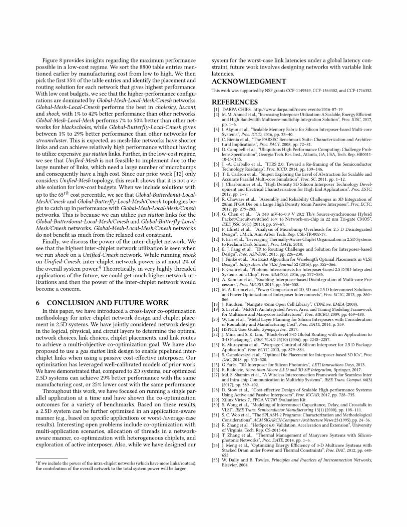
Figure 8 provides insights regarding the maximum performancepossible in a low-cost regime. We sort the 8800 table entries men-tioned earlier by manufacturing cost from low to high. We thenpick the �rst 35% of the table entries and identify the placement androuting solution for each network that gives highest performance.With low cost budgets, we see that the higher-performance con�gu-rations are dominated by Global-Mesh-Local-Mesh/Cmesh networks.Global-Mesh-Local-Cmesh performs the best in cholesky, lu.cont,and shock, with 1% to 42% better performance than other networks.Global-Mesh-Local-Mesh performs 7% to 50% better than other net-works for blackscholes, while Global-Butter�y-Local-Cmesh givesbetween 1% to 29% better performance than other networks forstreamcluster. This is expected, as mesh-like networks have shorterlinks and can achieve relatively high performance without havingto utilize expensive gas station links. Further, in the low-cost regime,we see that Uni�ed-Mesh is not feasible to implement due to thelarge number of links, which need a large number of microbumpsand consequently have a high cost. Since our prior work [12] onlyconsiders Uni�ed-Mesh topology, this result shows that it is not a vi-able solution for low-cost budgets. When we include solutions withup to the 65th cost percentile, we see that Global-Butterdonut-Local-Mesh/Cmesh and Global-Butter�y-Local-Mesh/Cmesh topologies be-gin to catch up in performancewithGlobal-Mesh-Local-Mesh/Cmeshnetworks. This is because we can utilize gas station links for theGlobal-Butterdonut-Local-Mesh/Cmesh and Global-Butter�y-Local-Mesh/Cmesh networks. Global-Mesh-Local-Mesh/Cmesh networksdo not bene�t as much from the relaxed cost constraint.
Finally, we discuss the power of the inter-chiplet network. Wesee that the highest inter-chiplet network utilization is seen whenwe run shock on a Uni�ed-Cmesh network. While running shockon Uni�ed-Cmesh, inter-chiplet network power is at most 2% ofthe overall system power.4 Theoretically, in very highly threadedapplications of the future, we could get much higher network uti-lizations and then the power of the inter-chiplet network wouldbecome a concern.
6 CONCLUSION AND FUTUREWORKIn this paper, we have introduced a cross-layer co-optimization
methodology for inter-chiplet network design and chiplet place-ment in 2.5D systems. We have jointly considered network designin the logical, physical, and circuit layers to determine the optimalnetwork choices, link choices, chiplet placements, and link routesto achieve a multi-objective co-optimization goal. We have alsoproposed to use a gas station link design to enable pipelined inter-chiplet links when using a passive cost-e�ective interposer. Ouroptimization has leveraged well-calibrated models of prior work.We have demonstrated that, compared to 2D systems, our optimized2.5D systems can achieve 29% better performance with the samemanufacturing cost, or 25% lower cost with the same performance.
Throughout this work, we have focused on running a single par-allel application at a time and have shown the co-optimizationoutcomes for a variety of benchmarks. Based on these results,a 2.5D system can be further optimized in an application-awaremanner (e.g., based on speci�c applications or worst-/average-caseresults). Interesting open problems include co-optimization withmulti-application scenarios, allocation of threads in a network-aware manner, co-optimization with heterogeneous chiplets, andexploration of active interposer. Also, while we have designed our
4If we include the power of the intra-chiplet networks (which have more links/routers),the contribution of the overall network to the total system power will be larger.
system for the worst-case link latencies under a global latency con-straint, future work involves designing networks with variable linklatencies.ACKNOWLEDGMENTThis work was supported by NSF grants CCF-1149549, CCF-1564302, and CCF-1716352.
REFERENCES[1] DARPA CHIPS. http://www.darpa.mil/news-events/2016-07-19[2] M.M. Ahmed et al., “Increasing Interposer Utilization: A Scalable, Energy E�cient
and High Bandwidth Multicore-multichip Integration Solution”, Proc. IGSC, 2017,pp. 1–6.
[3] I. Akgun et al., “Scalable Memory Fabric for Silicon Interposer-based Multi-coreSystems”, Proc. ICCD, 2016, pp. 33–40.
[4] C. Bienia et al., “The PARSEC Benchmark Suite: Characterization and Architec-tural Implications”, Proc. PACT, 2008, pp. 72–81.
[5] D. Campbell et al., “Ubiquitous High Performance Computing: Challenge Prob-lems Speci�cation”, Georgia Tech. Res. Inst., Atlanta, GA, USA, Tech. Rep. HR0011-10-C-0145.
[6] J. -A. Carballo et al., “ITRS 2.0: Toward a Re-framing of the SemiconductorTechnology Roadmap”, Proc. ICCD, 2014, pp. 139–146.
[7] T. E. Carlson et al., “Sniper: Exploring the Level of Abstraction for Scalable andAccurate Parallel Multi-core Simulation”, Proc. SC, 2011, pp. 1–12.
[8] J. Charbonnier et al., “High Density 3D Silicon Interposer Technology Devel-opment and Electrical Characterization for High End Applications”, Proc. ESTC,2012, pp. 1–7.
[9] R. Chaware et al., “Assembly and Reliability Challenges in 3D Integration of28nm FPGA Die on a Large High Density 65nm Passive Interposer”, Proc. ECTC,2012, pp. 279–283.
[10] G. Chen et al., “A 340 mV-to-0.9 V 20.2 Tb/s Source-synchronous HybridPacket/Circuit-switched 16⇥ 16 Network-on-chip in 22 nm Tri-gate CMOS”,IEEE JSSC 50(1) (2015), pp. 59–67.
[11] P. Ehrett et al., “Analysis of Microbump Overheads for 2.5 D DisintegratedDesign”, UMich. Ann Arbor Tech. Rep. CSE-TR-002-17.
[12] F. Eris et al., “Leveraging Thermally-Aware Chiplet Organization in 2.5D Systemsto Reclaim Dark Silicon”, Proc. DATE, 2018.
[13] E. J. Fang et al., “IR to Routing Challenge and Solution for Interposer-basedDesign”, Proc. ASP-DAC, 2015, pp. 226–230.
[14] J. Funke et al., “An Exact Algorithm for Wirelength Optimal Placements in VLSIDesign”, Integration, the VLSI Journal 52 (2016), pp. 355–366.
[15] P. Grani et al., “Photonic Interconnects for Interposer-based 2.5 D/3D IntegratedSystems on a Chip”, Proc. MEMSYS, 2016, pp. 377–386.
[16] A. Kannan et al., “Enabling Interposer-based Disintegration of Multi-core Pro-cessors”, Proc. MICRO, 2015, pp. 546–558.
[17] M. A. Karim et al., “Power Comparison of 2D, 3D and 2.5 D Interconnect Solutionsand Power Optimization of Iinterposer Interconnects”, Proc. ECTC, 2013, pp. 860–866.
[18] J. Knudsen, “Nangate 45nm Open Cell Library”, CDNLive, EMEA (2008).[19] S. Li et al., “McPAT: An Integrated Power, Area, and Timing Modeling Framework
for Multicore and Manycore architectures”, Proc. MICRO, 2009, pp. 469–480.[20] W. Liu et al., “Metal Layer Planning for Silicon Interposers with Consideration
of Routability and Manufacturing Cost”, Proc. DATE, 2014, p. 359.[21] HSPICE User Guide, Synopsys Inc., 2017.[22] J. Minz and S. K. Lim, “Block-level 3-D Global Routing with an Application to
3-D Packaging”, IEEE TCAD 25(10) (2006), pp. 2248–2257.[23] K. Murayama et al., “Warpage Control of Silicon Interposer for 2.5 D Package
Application”, Proc. ECTC, 2013, pp. 879–884.[24] S. Osmolovskyi et al., “Optimal Die Placement for Interposer-based 3D ICs”, Proc.
DAC, 2018, pp. 513–520.[25] G Parès, “3D Interposer for Silicon Photonics”, LETI Innovations Days, 2013.[26] R. Radojcic, More-than-Moore 2.5 D and 3D SiP Integration, Springer, 2017.[27] Md. S. Shamim et al., “A Wireless Interconnection Framework for Seamless Inter
and Intra-chip Communication in Multichip Systems”, IEEE Trans. Comput. 66(3)(2017), pp. 389–402.
[28] D. Stow et al., “Cost-e�ective Design of Scalable High-performance SystemsUsing Active and Passive Interposers”, Proc. ICCAD, 2017, pp. 728–735.
[29] Xilinx Virtex 7, FPGA VC707 Evaluation Kit.[30] S. Wong et al., “Modeling of Interconnect Capacitance, Delay, and Crosstalk in
VLSI”, IEEE Trans. Semiconductor Manufacturing 13(1) (2000), pp. 108–111.[31] S. C. Woo et al., “The SPLASH-2 Programs: Characterization and Methodological
Considerations”,ACM SIGARCH Computer Architecture News 23 (1995), pp. 24–36.[32] R. Zhang et al., “HotSpot 6.0: Validation, Acceleration and Extension”, University
of Virginia, Tech. Rep. CS-2015-04.[33] T. Zhang et al., “Thermal Management of Manycore Systems with Silicon-
photonic Networks”, Proc. DATE, 2014, pp. 1–6.[34] J. Meng et al., “Optimizing Energy E�ciency of 3-D Multicore Systems with
Stacked Dram under Power and Thermal Constraints”, Proc. DAC, 2012, pp. 648-655.
[35] W. Dally and B. Towles, Principles and Practices of Interconnection Networks,Elsevier, 2004.