UNIVERSITY OF ALABAMA

Department of Physics and Astronomy

PH 126 / LeClair Fall 2009

A Crash Course in Fluid Dynamics

Contents

1 The Continuity Equation 21.1 The Continuity equation in spherical coordinates . . . . . . . . . . . . . . . . . . . . . . 4

2 Static fluids 5

3 Moving fluids: Equations of motion without viscosity (“Dry Water”) 63.0.1 Rotation . . . . . . . . . . . . . . . . . . . . . . . . . . . . . . . . . . . . . . . 83.0.2 Irrotational Fluids . . . . . . . . . . . . . . . . . . . . . . . . . . . . . . . . . . 93.0.3 Steady flows and Bernoulli’s equation . . . . . . . . . . . . . . . . . . . . . . . . 103.0.4 Example: water draining from a tank . . . . . . . . . . . . . . . . . . . . . . . . 10

4 Viscosity 11

5 Tensors 135.1 Conductivity tensor for the Hall effect . . . . . . . . . . . . . . . . . . . . . . . . . . . 155.2 Other examples of tensors . . . . . . . . . . . . . . . . . . . . . . . . . . . . . . . . . . 17

6 The Stress Tensor 176.1 The Maxwell stress tensor . . . . . . . . . . . . . . . . . . . . . . . . . . . . . . . . . . 20

7 Viscosity and stress in three dimensions 21

8 Viscous forces in three dimensions 23

9 The equation of motion with viscosity for incompressible fluids 269.1 Steady flow through a long cylindrical pipe . . . . . . . . . . . . . . . . . . . . . . . . . 279.2 Stoke’s flow around a solid sphere . . . . . . . . . . . . . . . . . . . . . . . . . . . . . . 29

1

In your introductory mechanics class, you have no doubt dealt with hydrostatics, and the forces andenergy of fluids which are at rest. The purpose of these notes is to introduce you to the problem of amoving fluid, and derive the equations relating the pressure and velocity distribution within a fluid. Asa special case, we will derive Bernoulli’s equation for incompressible, viscosity-free fluids, and as a moregeneral case we will derive the Navier-Stokes equation for incompressible fluids. We will then apply theseresults to a (relatively) simple case, the flow of low-speed air past a dense sphere.

1 The Continuity Equation

The starting pointi for our treatment of fluids will be the derivation of the continuity equation for a fluid.A continuity equation, if you haven’t heard the term, is nothing more than an equation that expresses aconservation law. In the case of continuous media, such as a fluid, our conservation law is conservationof matter. In electromagnetism, one continuity equation expresses conservation of charge.

Qualitatively, a general continuity equation for mass reads something like this:

(rate of mass accumulation) + (rate of mass out) − (rate of mass in) = 0 (1)

If you replace “mass” with “charge” or “momentum” you can imagine all sorts of continuity equationsthat fall under the general heading of “conservation of stuff.” We can be a bit more precise by applyingour continuity equation to a specific volume of space V , which is defined by a bounding surface S. Inthis case, the net rate at which mass accumulates inside V depends on the net rate at which mass passesthrough S, either coming in or going out:

(rate of mass accumulation in V) + (net rate of mass crossing S) = 0 (2)

This is basically just bookkeeping. If the amount of mass in V is static, then it must be true that theamount of matter entering through S is the same as the amount of matter leaving through S. If theamount of mass in V is increasing, then there must be a net flow of matter in through S. Since we wishto deal with continuous substances like fluids, rather than the individual particles we usually deal with inmechanics, it is most convenient to put our equations in terms of the density of the substance ρ.

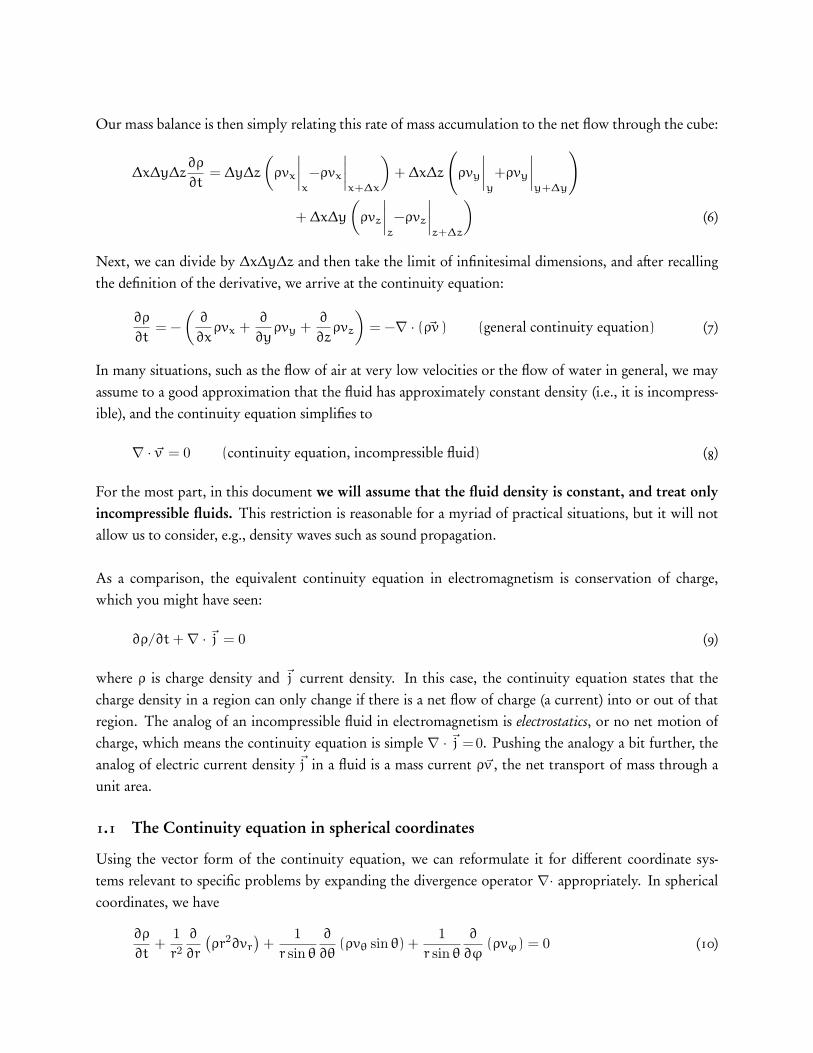
Consider a tiny cube of our substance of dimensions ∆x ∆y∆z. The mass of this cube is simply ρ ∆x∆y ∆z.If we have a net flow of our substance through this cube, let’s say in the x direction, how does the massof the cube change with time? If the substance is incompressible, and the cube remains completely full,then the mass doesn’t change, of course. However, in the general case, we just need to keep track of howmuch mass is in the cube at any moment, and how much mass enters and leaves.

iMuch of this document is based on Ch. 2 of D.R. Poirier and G.H. Geiger, Transport Phenomena in Materials Processing,TMS, Warrendale, PA, 1994) and Ch. 40-41 of the Feynman Lectures on Physics, vol. II

x

yz

∆x

∆y

∆z

(x,y, z)

(x + ∆x,y + ∆y, z + ∆z)

(ρvx)|x (ρvx)|x+∆x

Figure 1: Volume element fixed in space with fluid flowing through it.

We will presume that our cube is nicely aligned along the x, y, and z axes, and that there is a net flowof our substance with velocity ~v , as shown in Fig. 1. We will assume that the density of our substanceis constant. If we look first at the faces of the cube perpendicular to the x axis (i.e., the faces whosearea normals are parallel to the x axis), the net flow through the cube along the x axis can be found becomparing the rate at which mass enters one side and leaves the other. The rate of mass flowing throughthe left side face at x is

∂m

∂t

∣∣∣∣x

=∂

∂t(ρV)

∣∣∣∣x

=∂

∂t(ρ∆x∆y∆z)

∣∣∣∣x

= ∆y∆z (ρvx)

∣∣∣∣x

(3)

This is just the familiar result that the mass flow rate through a pipe is product of the velocity of theflow, the fluid density, and the pipe’s cross-sectional area. In the same manner, we can find the flow ratethrough the right side face at x + ∆x,

∂m

∂t

∣∣∣∣x+∆x

= ∆y∆z (ρvx)

∣∣∣∣x+∆x

(4)

We can proceed similarly for the other two pairs of faces perpendicular to the y and z axes, and then addup all the terms for fluid entering or leaving the cube to come up with a mass balance. If, when we addup the rates for all the sides, we have a non-zero result, then we must be either accumulating mass insideour cube, or it is experiencing a net loss in mass. Either way, the accumulation in mass inside our cube ofconstant volume can only reflect a change in density,

(mass accumulation) =∂

∂t(ρV) = ∆x∆y∆z

∂ρ

∂t(5)

Our mass balance is then simply relating this rate of mass accumulation to the net flow through the cube:

∆x∆y∆z∂ρ

∂t= ∆y∆z

(ρvx

∣∣∣∣x

−ρvx

∣∣∣∣x+∆x

)+ ∆x∆z

(ρvy

∣∣∣∣y

+ρvy

∣∣∣∣y+∆y

)

+ ∆x∆y

(ρvz

∣∣∣∣z

−ρvz

∣∣∣∣z+∆z

)(6)

Next, we can divide by ∆x∆y∆z and then take the limit of infinitesimal dimensions, and after recallingthe definition of the derivative, we arrive at the continuity equation:

∂ρ

∂t= −

(∂

∂xρvx +

∂

∂yρvy +

∂

∂zρvz

)= −∇ · ( ~ρv ) (general continuity equation) (7)

In many situations, such as the flow of air at very low velocities or the flow of water in general, we mayassume to a good approximation that the fluid has approximately constant density (i.e., it is incompress-ible), and the continuity equation simplifies to

∇ · ~v = 0 (continuity equation, incompressible fluid) (8)

For the most part, in this document we will assume that the fluid density is constant, and treat onlyincompressible fluids. This restriction is reasonable for a myriad of practical situations, but it will notallow us to consider, e.g., density waves such as sound propagation.

As a comparison, the equivalent continuity equation in electromagnetism is conservation of charge,which you might have seen:

∂ρ/∂t +∇ · ~j = 0 (9)

where ρ is charge density and ~j current density. In this case, the continuity equation states that thecharge density in a region can only change if there is a net flow of charge (a current) into or out of thatregion. The analog of an incompressible fluid in electromagnetism is electrostatics, or no net motion ofcharge, which means the continuity equation is simple ∇ · ~j = 0. Pushing the analogy a bit further, theanalog of electric current density ~j in a fluid is a mass current ρ~v , the net transport of mass through aunit area.

1.1 The Continuity equation in spherical coordinates

Using the vector form of the continuity equation, we can reformulate it for different coordinate sys-tems relevant to specific problems by expanding the divergence operator ∇· appropriately. In sphericalcoordinates, we have

∂ρ

∂t+

1r2

∂

∂r

(ρr2∂vr

)+

1r sin θ

∂

∂θ(ρvθ sin θ) +

1r sin θ

∂

∂ϕ(ρvϕ) = 0 (10)

Our main problem of interest is the slow flow of a fluid past a dense sphere. If the fluid flow is along thez axis, the problem is symmetric about the z axis, and we may neglect the ϕ components of velocity. Inother words, the problem is essentially two-dimensional, thanks to the rotational symmetry about the z

axis. In this special case,

∂ρ

∂t+

1r2

∂

∂r

(ρr2∂vr

)+

1r sin θ

∂

∂θ(ρvθ sin θ) = 0 (11)

2 Static fluids

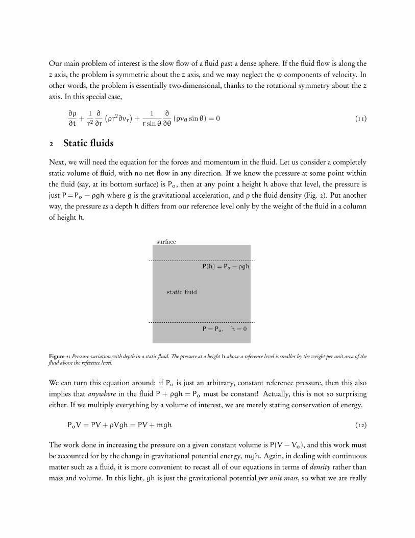
Next, we will need the equation for the forces and momentum in the fluid. Let us consider a completelystatic volume of fluid, with no net flow in any direction. If we know the pressure at some point withinthe fluid (say, at its bottom surface) is Po, then at any point a height h above that level, the pressure isjust P =Po − ρgh where g is the gravitational acceleration, and ρ the fluid density (Fig. 2). Put anotherway, the pressure as a depth h differs from our reference level only by the weight of the fluid in a columnof height h.

static fluid

surface

P(h) = Po − ρgh

P = Po, h = 0

Figure 2: Pressure variation with depth in a static fluid. The pressure at a height h above a reference level is smaller by the weight per unit area of thefluid above the reference level.

We can turn this equation around: if Po is just an arbitrary, constant reference pressure, then this alsoimplies that anywhere in the fluid P + ρgh = Po must be constant! Actually, this is not so surprisingeither. If we multiply everything by a volume of interest, we are merely stating conservation of energy.

PoV = PV + ρVgh = PV + mgh (12)

The work done in increasing the pressure on a given constant volume is P(V − Vo), and this work mustbe accounted for by the change in gravitational potential energy, mgh. Again, in dealing with continuousmatter such as a fluid, it is more convenient to recast all of our equations in terms of density rather thanmass and volume. In this light, gh is just the gravitational potential per unit mass, so what we are really

saying is that pressure plus gravitational potential is a constant for a static fluid, or that pressure itself is asort of volumetric potential. Thus, if we define a gravitational potential per unit mass φ=gh, we have

P + ρφ = const with φ = Ugrav/m = gh (13)

Now we have an energy balance for our static fluid, it is only a bit of mathematics to find a force balance.If we consider a one-dimensional fluid, we know that force is just the spatial derivative of the potentialenergy, Fx =−dU/dx. The same will hold true of the potential energy per unit volume, which amountsto taking the spatial derivative of both sides of Eq. 13. In one dimension, this gives

∂P

∂x+

∂

∂x(ρφ) = 0 (14)

If we consider only fluids of constant density (incompressible fluids), this simplifies to

∂P

∂x+ ρ

∂φ

∂x= 0 (15)

In three dimensions, we need only replace the spatial derivative with a gradient:

∇P +∇ (ρφ) = 0 (compressible) (16)

∇P + ρ∇φ = 0 (incompressible) (17)

This is nothing more than a Newton’s law force balance for our stationary fluid, if we recognize thatρ∇φ is the force (per unit volume): in static equilibrium, the force per unit volume is precisely balancedby a gradient in pressure.

This equation is the complete description of hydrostatics, though it is quite a bit more complicated thanit looks: there is no general solution. If the density of the fluid varies spatially (∇ρ=0 somewhere), ourcontinuity equation above tells us that there is no way that a static equilibrium can be maintained, wemust have also have time-varying density. ii Only if ρ is constant in space do we have a simple solutionfor hydrostatics, viz., P + ρϕ=const.

3 Moving fluids: Equations of motion without viscosity (“Dry Water”)

What to do if the fluid is not static? We already know the continuity equation in general, but we still needto consider a more general force balance for our fluid. What we have derived above is the equilibriumcondition for a static fluid, generalizing just means letting the pressure and potential gradient terms

iiStrictly, for a fluid of constant density, a spatially-varying density in Eq. 7 implies that the velocity field must have zerodivergence, or be zero everywhere to have a density which does not vary in time. Only the case v = 0 corresponds to a trulystatic situation, and thus, if ρ has any spatial variation, a time variation is implied.

become unbalanced to yield a net acceleration. In the absence of viscous forces, this would simply be

ρ× (acceleration) = −∇P − ρ∇φ (18)

The left side is the net force per unit volume, and the first two terms on the right are our pressure andpotential gradients. Already, if these terms on the right are unbalanced (e.g., if we have a spatially-varyingdensity) we will have a net acceleration of the fluid, and hence motion. What does the acceleration termlook like?

What we really need to find is ∆~v /∆t for infinitesimal ∆t, that is our acceleration. Just from the math-ematics of partial derivatives, we can say quite a lot already. Say we know the velocity of a infinitesimalvolume of fluid at some particular point in space and time, ~v (x,y, z, t). What is the velocity of the samebit of fluid at some later time t+∆t when the bit of fluid is at a neighboring point (x+∆x,y+∆y, z+∆z)?From the definition of partial derivatives, for small changes in x, y, z, and t (i.e., to first order) we canwrite the change in velocity as

∆~v = ~v (x + ∆x,y + ∆y, z + ∆z, t + ∆t) − ~v (x,y, z, t) (19)

=∂~v

∂x∆x +

∂~v

∂y∆y +

∂~v

∂z∆z +

∂~v

∂t∆t (20)

This is not incredibly useful, as such, but we can multiply and divide every spatial derivative by ∆t toput this in a more interesting form:

∆~v =∂~v

∂x∆x +

∂~v

∂y∆y +

∂~v

∂z∆z +

∂~v

∂t∆t (21)

=∂~v

∂x

∆x

∆t∆t +

∂~v

∂y

∆y

∆t∆t +

∂~v

∂z

∆z

∆t∆t +

∂~v

∂t∆t (22)

=∂~v

∂xvx∆t +

∂~v

∂yvy∆t +

∂~v

∂zvz∆t +

∂~v

∂t∆t (23)

=

(∂~v

∂xvx +

∂~v

∂yvy +

∂~v

∂zvz +

∂~v

∂t

)∆t (24)

The acceleration d~v /dt then becomes, in the limit ∆t→0,

d~v

dt=

∂~v

∂xvx +

∂~v

∂yvy +

∂~v

∂zvz +

∂~v

∂t(25)

This might not look like much, but if we look and rearrange it carefully we can recognize a nicer vector

form:

d~v

dt= vx

∂~v

∂x+ vy

∂~v

∂y+ vz

∂~v

∂z+

∂~v

∂t(26)

=

[(vx x + vy y + vz z) ·

(∂

∂xx +

∂

∂yy +

∂

∂zz

)]~v +

∂~v

∂t= (~v · ∇) ~v +

∂~v

∂t(27)

Can you see why it must be (~v · ∇) ~v and not, e.g., ~v · (∇~v )? (If for no other reason, the former is avector while the latter is a scalar!)

Having found the acceleration, in the absence of viscous forces our equation of motion is complete:

d~v

dt= ρ (~v · ∇) ~v + ρ

∂~v

∂t= −∇P − ρ∇φ (equation of motion, no viscosity) (28)

3.0.1 Rotation

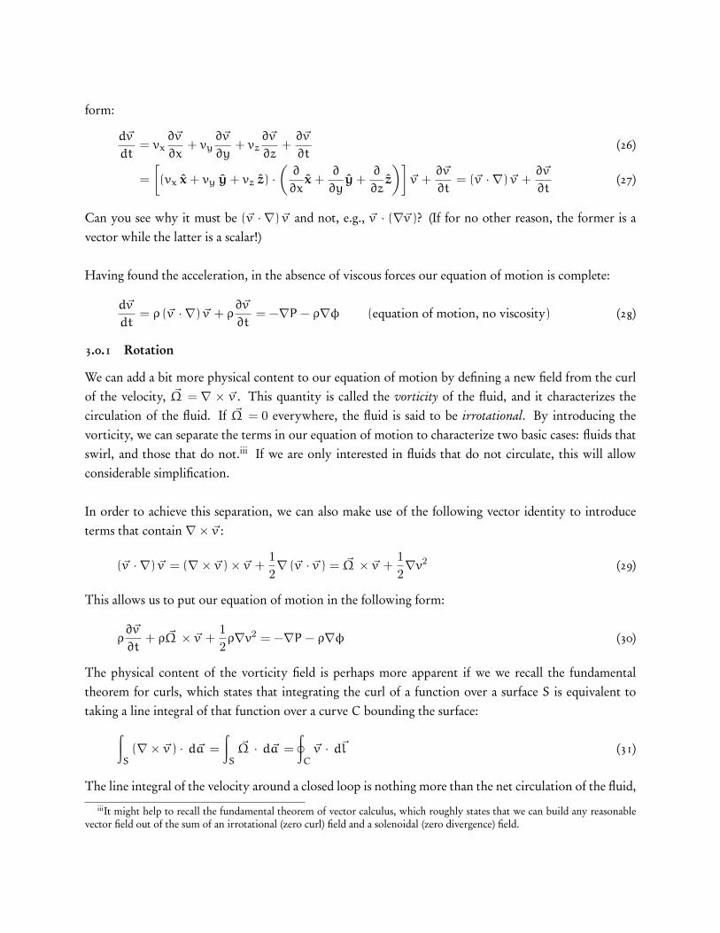
We can add a bit more physical content to our equation of motion by defining a new field from the curlof the velocity, ~Ω = ∇ × ~v . This quantity is called the vorticity of the fluid, and it characterizes thecirculation of the fluid. If ~Ω = 0 everywhere, the fluid is said to be irrotational. By introducing thevorticity, we can separate the terms in our equation of motion to characterize two basic cases: fluids thatswirl, and those that do not.iii If we are only interested in fluids that do not circulate, this will allowconsiderable simplification.

In order to achieve this separation, we can also make use of the following vector identity to introduceterms that contain ∇× ~v :

(~v · ∇) ~v = (∇× ~v )× ~v +12∇ (~v · ~v ) = ~Ω × ~v +

12∇v2 (29)

This allows us to put our equation of motion in the following form:

ρ∂~v

∂t+ ρ ~Ω × ~v +

12ρ∇v2 = −∇P − ρ∇φ (30)

The physical content of the vorticity field is perhaps more apparent if we we recall the fundamentaltheorem for curls, which states that integrating the curl of a function over a surface S is equivalent totaking a line integral of that function over a curve C bounding the surface:∫

S(∇× ~v ) · d~a =

∫S

~Ω · d~a =

∮C

~v · d~l (31)

The line integral of the velocity around a closed loop is nothing more than the net circulation of the fluid,iiiIt might help to recall the fundamental theorem of vector calculus, which roughly states that we can build any reasonable

vector field out of the sum of an irrotational (zero curl) field and a solenoidal (zero divergence) field.

so what this tells us is that the vorticity ~Ω is just the net circulation of the fluid around an infinitesimalclosed loop. Consider the case where we have pure rotational motion of a fluid, such as a perfect circularflow of fluid inside a bucket. At a given radius r from the center of rotation, this gives 2πrv=πr2Ω, orω=Ω/2. The angular velocity of the fluid (or a small particle placed in the fluid) at any given radius isjust half the vorticity.

We can go still further with vorticity. If we are only interested in the velocity field in the fluid, we caneliminate pressure from Eq. 30. If we take the curl of both sides of Eq. 30, and remember that∇×(∇f)=0for any f, we have

ρ∇× ∂~v

∂t+ ρ∇×

(~Ω × ~v

)= 0 (32)

or∂ ~Ω

∂t+∇×

(~Ω × ~v

)= 0 (33)

Along with the definition of vorticity ~Ω =∇× ~v and our continuity equation∇ · ~v =0, this equation issufficient to find the velocity field of our fluid. From the form of these equations, if we know ~Ω at oneparticular time, that means we also know both the curl and divergence of ~v , which means knowledge of~Ω alone determines v. In fact, there is an even more striking consequence: if we have ~Ω =0 everywhereat some instant in time, then ∂ ~Ω /∂t=0 as well. If the fluid is irrotational at any time, it is irrotational atall times! As nice as this new equation is, we should not forget that we have thrown away all informationabout the pressure. We would still have to take our velocity field and use Eq. 30 to deduce anything aboutthe pressure.

As an aside, our equations in terms of vorticity have an interesting analogy with magnetism, where wehave

∇ · ~B = 0 ∇× ~B = µo~j ~B = ∇× ~A (34)

Thus, mathematically speaking, velocity is analogous to magnetic field, and vorticity is analogous tocurrent density. Knowledge of the current density throughout space allows us to determine the magneticfield, just as knowledge of the vorticity allows us to determine the velocity.

3.0.2 Irrotational Fluids

Now, taking advantage of this new form, we can consider only irrotational fluids for which ~Ω =0 (as isthe case in our experiment), in which case we have the simpler result

ρ∂~v

∂t+

12ρ∇v2 = −∇P − ρ∇φ (equation of motion, no viscosity, irrotational) (35)

At this point, we can make another analogy with electromagnetism. The conditions of zero rotation and

continuity actually give us enough to solve for the velocity field by themselves:

∇ · ~v = 0 ∇× ~v = 0 (36)

This is just like Maxwell’s equations for ~E and ~B in free space. This is handy: for an irrotational,incompressible fluid the boundary value problems are often the same as ones we have already solved.What’s more, these equations are linear differential equations, unlike our more general expressions forfluid flow. This is only true for incompressible fluids in irrotational flow. Since the governing equationsare linear, that means that the solutions obey superposition: if we have two solutions to the equations,then their sum (or difference) is also a solution, just like in electromagnetism.

3.0.3 Steady flows and Bernoulli’s equation

Finally, there is one more simplification we can make for many reasonable cases: the assumption of steadyflow. This doesn’t mean we have nothing happening, it is merely the condition that we have motion ofthe fluid at constant velocity, ∂~v /∂t=0. In this case,

12ρ∇v2 = −∇P − ρ∇φ (equation of motion, no viscosity, irrotational, steady flow) (37)

Since every term in this equation involves a gradient, we may simply integrate both sides to get rid of agradient from every term, and once we remember to add in an integration constant, we have

12ρv2 + P + ρφ = (const) (38)

If we multiply through by a volume of interest, we recover something recognizable:

12mv2 + PV + mgh = (const) (39)

This is Bernoulli’s theorem, which is just a statement of conservation of energy for an irrotational fluid.Compare this to our starting point for a static fluid, P + ρφ = (const.), and you will see that the newterm 1

2ρv2 is nothing more than the kinetic energy of the moving fluid!

3.0.4 Example: water draining from a tank

As a quick practical example of what we can do with this, let’s consider a case you have all dealt with:water draining in the bathtub. We’ll imagine that we have a cylindrical bathtub of radius R, with a drainplug at the bottom in the exact center of the tub. Now we’ll fill up the tub, stir it up to get it circulat-ing, and pull the drain plug. We know that at first the water will form a nice spiral circulating downthe drain, but the rotation will die out due to viscosity after a short time.iv After the flow becomes ir-

ivWhy don’t you have to stir the tub to see this effect? It has nothing to do with what hemisphere you’re in or the Corioliseffect, it is simply a result of the pipes leading away from the tub having turns in them.

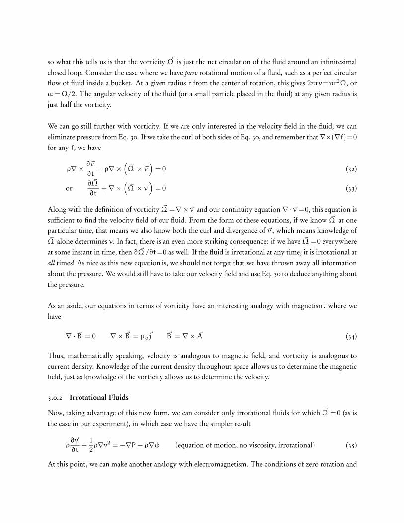
rotational due to viscous forces, what remains is still a nice conical shape, however. But what is the shape?

Within a given vertical plane, we can calculate the net circulation at a radial distance r from the center asin Eq. 31,

∮~v · d~r =2πrvθ, where vθ is the tangential velocity. Once we are in the regime of irrotational

flow, however, the circulation can’t depend on the radial distance.v Thus, we must have 2πrvθ =constant,and this can only be true if the tangential velocity is proportional to 1/r. If we express the continuityequation ∇ · ~v =0 in cylindrical coordinates, we can find the radial component of the velocity:

∇ · ~v =1r

∂

∂r(rvr) +

1r

∂vθ

∂θ= 0 =⇒ rvr = (constant) (40)

Thus, the radial velocity must also be proportional to 1/r. At the air-water boundary, we know thatthe pressure is simply atmospheric pressure, a constant. Since our fluid is irrotational, incompressible,and experiencing steady flow at a given radial position, we can use Bernoulli’s equation to express energyconservation at a given radial position r and height z:

12mv2 + mgz = (const) (41)

Since we know v∝1/r, this means that z∝1/r2, and the shape of our draining water surface thus obeysthe curve z(r)=C/r2.

4 Viscosity

Adding a viscous (drag) force to our equation of motion is not much of a problem, in principle. If wehave a viscous force ~f v per unit volume, then Newton’s law yields

ρ (~v · ∇) ~v + ρ∂~v

∂t= −∇P − ρ∇φ + ~f v (42)

We simply have to add in the net viscous force per unit volume to the forces due to a pressure gradientand a height variation. The problem is, how do we model the viscous force?

Our model of fluid flow thus far basically ignores the presence of any resistive forces, or forces perpen-dicular to the direction of the fluid flow. In other words, our first model assumes that the fluid will putup no resistance to being pushed around, which is clearly unrealistic. This is not even realistic for a solid:when we deform a solid, we know that it will produce a restoring force proportional to the strain itexperiences, giving rise to Hooke’s law macroscopically. Real fluids will also react to an applied force orpressure, but more important in this case than the amount of strain is the rate at which strain is produced.For example, in most fluids it is easier to move slowly than it is to move rapidly – think about swimming

vYou might think that the circulation has to be zero, but that is not quite true because we include the origin in our surface.The curl of the velocity is zero everywhere except the origin, and this gives a constant contribution to the integral of∇×~v overa surface including the origin.

or stirring a jar of thick syrup.

Perhaps more importantly, when we consider a continuous substance like a fluid we have to considerlateral or shear forces tangential to the direction of motion. If you stir a jar of syrup along one direction,there is clearly a fluid flow along the directions tangential to the motion, meaning there must be forcesnot just parallel to the fluid motion but in the transverse directions as well. This a type of force you haveprobably not encountered before, and one which requires careful treatment.

Thinking about the problem another way, our previous model also ignored any interactions between amoving fluid and a solid surface it encounters. In fact, it would have all but impossible to do so withoutsome sort of empirical guidance or at least a hint at the answer. In this, we are lucky, however. Oneimportant experimental fact severely constrains models of viscous forces: the velocity of a fluid is exactlyzero at the boundary of a solid surface. This is not an obvious fact, but one you can easily verify: how elsewould your ceiling fan blades have dust on them? Shouldn’t it blow off?

With this fact, we can attempt a model of viscous forces. Image that we have two flat parallel plates ofarea A immersed in an initially stationary fluid, separated by a distance d. We hold one plate at rest in thefluid, and move the other plate at velocity vo through the fluid. In a fluid without viscosity, the movingplate would not disturb the fluid at all, and the fluid velocity would be zero everywhere. However, if therelative velocity of fluid and plate must be zero at each plate’s surface, that means that the fluid velocityvaries from 0 to vo moving from the stationary to the moving plate! At the surface of the moving plate,the fluid must have velocity vo, and at the surface of the stationary plate, it must have v=0.

d

v = 0

v

Fvo

Figure 3: Viscous drag between two parallel plates in a fluid.

If you measure the force required to keep the top plate moving, it turns out to be proportional to thevelocity of the plate and its area divided by the spacing between the plates at low velocities (low Reynold’s

numbers).

F = ηvoA

d(43)

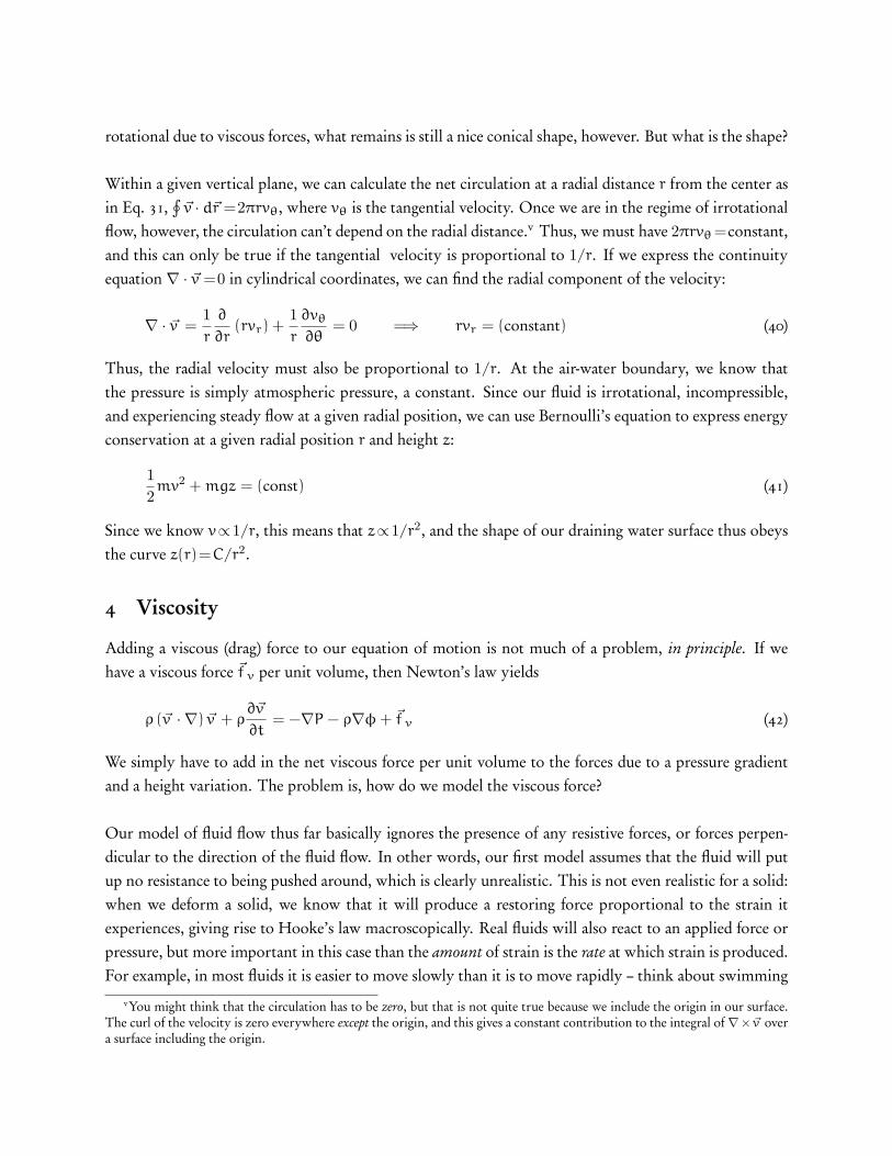
The constant of proportionality η is known as the coefficient of viscosity, and to some extent it is ameasure of how much force must be supplied to produce motion in a fluid. Noting that power is ~F · ~v ,you can see that the power required to maintain a speed v in a fluid scales as ηv2. What is interestingabout this relationship is that the force, along the axis of motion, depends on the transverse area of theplate. This is quite different from any force we’ve encountered so far!

In moving beyond a single dimension, we also have our previous and related problem to consider: if wepress on a fluid in one direction, it will move in all directions, not just along the direction of the appliedforce. This is in sharp contrast to our usual considerations of infinitesimal particles, or rigid objects.What do we do when the object can “squish?” In the example above, the moving plate will displace thefluid it is moving through, imparting velocity in the directions perpendicular to the motion of the plate.Evidently, what we lack is a way to relate an applied along one direction with an induced force alonganother. The mathematical tool we are missing is the tensor, a generalization of vectors and scalars whichturns out to be indispensable for many areas of physics.

5 Tensors

So far as we need them, a tensor is a set of numbers (or a matrix) that when multiplied by a vector givesback a new vector. Of course, this much can be accomplished by vector or scalar multiplication, butwhat makes tensors special is that the two vectors need not be simply parallel or perpendicular. This isexactly what we need to understand stress and pressure in materials: relating a displacement or force inone direction to a resulting force along a different direction, particularly when materials are allowed todeform. A close analogy to the type of mathematical object we need is the rotation matrix: a multiplyinga given vector by a rotation matrix gives a new vector of the same length, but pointing in a new direc-tion. A tensor is in a sense a more general type of matrix, in which both the length and direction of theresulting vector are generally different.

As an example, let’s say we want to consider the conductivity of a material, σ. Ohm’s law states that thecurrent density is proportional to the electric field via the conductivity:

~j = σ~E (44)

In an isotropic, homogeneous material, σ is just a scalar, a plain number, that characterizes how muchcurrent density results from a specific electric field. As such, a scalar conductivity results in a currentdensity which is always parallel to the electric field. In many materials, this is a perfectly reasonable

assumption. However, this is clearly a simplification: what about crystals? In a perfect crystal, we havea symmetric arrangement of atoms which is clearly not isotropic, and it is unphysical to expect the con-ductivity to be the same along every direction in the crystal. If we have a simple cubic crystal, it wouldbe reasonable to expect the conductivity to be the same along all three crystallographic directions, butwe would certainly expect a different conductivity along other directions.

Consider a simple two-dimensional crystal, with a square grid of atoms along the x and y directions. Ifthe spacing of atoms along x and y is the same, we expect that a given electric field applied along the x

or y direction would lead to the same current density. However, if we applied the electric field along theline y = x, 45 with respect to the rows of atoms, we should expect a different current density. Thus,at the very least, our conductivity must be direction-dependent so long as the crystal is not isotropic!Moreover, this means that we can’t even reasonably expect that the current density is along the samedirection as the electric field. If the field is along the the line y=x, and we have different conductivities inthe x and y directions, we should expect that the resulting current density has both x and y components,and they will not be the same. Even in an isotropic material we have to worry about this to an extent,current will spread out in all directions in a uniform conductor.

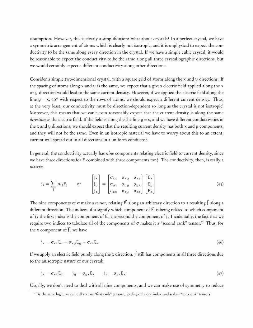
In general, the conductivity actually has nine components relating electric field to current density, sincewe have three directions for E combined with three components for j. The conductivity, then, is really amatrix:

ji =∑

j

σijEj or

jx

jy

jz

=

σxx σxy σxz

σyx σyy σyz

σzx σzy σzz

Ex

Ey

Ez

(45)

The nine components of σ make a tensor, relating ~E along an arbitrary direction to a resulting ~j along adifferent direction. The indices of σ signify which component of ~E is being related to which componentof ~j : the first index is the component of ~E , the second the component of ~j . Incidentally, the fact that werequire two indices to tabulate all of the components of σ makes it a “second rank” tensor.vi Thus, forthe x component of ~j , we have

jx = σxxEx + σxyEy + σxzEz (46)

If we apply an electric field purely along the x direction, ~j still has components in all three directions dueto the anisotropic nature of our crystal:

jx = σxxEx jy = σyxEx jz = σzxEx (47)

Usually, we don’t need to deal with all nine components, and we can make use of symmetry to reduceviBy the same logic, we can call vectors “first rank” tensors, needing only one index, and scalars “zero rank” tensors.

the number of independent components. For instance, the conductivity tensor is symmetric, meaningthat σij =σji. Applying an electric field Ex along the x axis leads to a current density jy along the y axis,and if we apply the same electric field along the y axis, we end up with the same current density alongthe x axis:

jy = σyxEx jx = σxyEy σxy = σyx (48)

In fact, it is possible to simplify the conductivity even further. Our choice of axes along which todecompose the electric field and conductivity vectors, and thus the conductivity tensor, was completelyarbitrary. For a second-rank tensor like conductivity, it is always possible to choose axes such that thetensor is diagonal, e.g., such that only σxx, σyy, and σzz are non-zero:jx

jy

jz

=

σxx 0 00 σyy 00 0 σzz

Ex

Ey

Ez

(49)

In a crystal, finding the diagonal representation of a tensor typically corresponds to choosing the naturalcrystallographic axes for decomposing the electric field and current density. Finally, in an isotropicmaterial, in which the conductivity is independent of direction, σxx =σyy =σzz, and we may treat theconductivity as a simple scalar.

5.1 Conductivity tensor for the Hall effect

Actually, we already know one simple situation in which a tensor conductivity is required even for anisotropic medium: the Hall effect. You used tensors without even knowing it! Imagine we have a sheetof uniform conductor lying in the xy plane, with an electric field Ey applied along the y axis. Thiswill impart a velocity, on average, of vy to each positive charge q in the conductor. In the absence of amagnetic field, Ohm’s law plus a free-electron model gives us the current density in the y direction:

jy = σyyEy with σyy =nq2τ

m(50)

Here n is the number of charge carriers per unit volume, m the mass and q the charge per carrier, and τ

the average time between collisions. Now, of course, we know that we need to label σ as a tensor. In thiscase, we need the component σyy when both current density and electric field are along y. Applyingan electric field along the x direction for our homogenous sample would lead us to σxx = σyy. If thereis no magnetic field, then this is the end of the story: σxy = σyx = 0, since there is no net force onthe charges in the directions perpendicular to E. Thus, our conductivity tensor is diagonal, and the diag-onal elements are all the same, which means we can treat the conductivity as a simple scalar. No problem.

Next, we add a magnetic field Bz in the +z direction in addition to the electric field in the y direction.

Now we have a transverse magnetic force on the charge carriers, FB =qvyBz, acting on positive chargesin the +x direction. This leads to a separation of charge along the x axis, which means there must bean electric field −Ex now. This electric field will give rise to a force opposing the charge separation:the stronger the magnetic field, the stronger the magnetic force, the larger the charge separation, butthe larger the electric field. At equilibrium, the two horizontal forces must be equal, qEx = qvyBz, orEx =vyBz. We could have arrived at this result far more quickly using the relativistic transformations ofthe fields: in the charges’ reference frame, traveling at velocity ~v , the magnetic field appears as an electricfield of magnitude ~E

′=~v × ~B .

This is the usual Hall effect you have seen in electromagnetism: a magnetic field applied orthogonal toa current gives rise to an electric field (or potential difference) along the third axis. What it means isthat now we have a “shear” component to our conductivity tensor: the electric field and current densityalong y in the presence of a magnetic field along z gives us an electric field along x! Even though theconductor itself is isotropic, the presence of a magnetic field breaks the symmetry of the problem, andthat is sufficient to require a tensor to relate ~j and ~E .

Now we just need to figure out what the new component of the conductivity is. Since in the field Bz wehave Ex resulting from jy, we can guess that it must be σyx. We have already related Ex and Bz, we canrelate Ex and jy by noting the relationship between current density and drift velocity: jy =nqvy. Thus,

Ex = vyBz =jyBz

nq(51)

jy =nq

BzEx = σyxEx =⇒ σyx =

nq

Bz(52)

What about σyx? If we were to apply the electric field along the x direction instead, but keep B in the z

direction, we would have a current density along the x direction, but the induced electric field would bealong −y rather than +y. This means σyx = σxy. In the presence of orthogonal electric and magneticfields, we can now write down the entire conductivity tensor:

σ =

[σxx σxy

−σxy σyy

]=

nq2τ

m

nq

Bz−nq

Bz

nq2τ

m

(53)

This conductivity tensor encompasses both normal Ohmic conduction and the Hall effect. If the fieldsare not orthogonal, this is not much of a problem, at least in two dimensions, since only the componentof ~B orthogonal to ~E will alter the conductivity in this simple picture.

5.2 Other examples of tensors

In fact, you’ve already encountered tensors many times, probably without knowing it. Generally speak-ing, if you need to relate two vectors, and they in general need not be strictly parallel or perpendicular,a tensor is probably involved. For instances, the moment of inertia is really a 2nd-rank tensor, sinceangular momentum and angular velocity are not in general parallel. Torque is also a 2nd-rank tensor, andanti-symmetric (τij =−τji), but happens to transform like a vector in three dimensions. For that reason,we usually just treat it as a vector (or pseudovector, really) since we can get away with it!

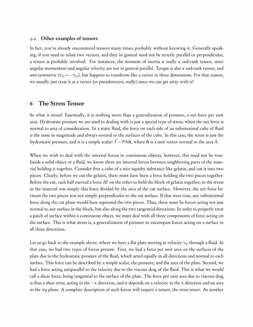
6 The Stress Tensor

So what is stress? Essentially, it is nothing more than a generalization of pressure, a net force per unitarea. Hydrostatc pressure we are used to dealing with is just a special type of stress, when the net force isnormal to area of consideration. In a static fluid, the force on each side of an infinitesimal cube of fluidis the same in magnitude and always normal to the surfaces of the cube. In this case, the stress is just thehydrostatic pressure, and it is a simple scalar: ~F =PAn, where n is a unit vector normal to the area A.

When we wish to deal with the internal forces in continuous objects, however, this need not be true.Inside a solid object or a fluid, we know there are internal forces between neighboring parts of the mate-rial holding it together. Consider first a cube of a nice squishy substance like gelatin, and cut it into twopieces. Clearly, before we cut the gelatin, there must have been a force holding the two pieces together.Before the cut, each half exerted a force ∆F on the other to hold the block of gelatin together, so the stressin the material was simply this force divided by the area of the cut surface. However, the net force be-tween the two pieces was not simply perpendicular to the cut surface. If that were true, any infinitesimalforce along the cut plane would have separated the two pieces. Thus, there must be forces acting not justnormal to any surface in the block, but also along the two tangential directions. In order to properly treata patch of surface within a continuous object, we must deal with all three components of force acting onthe surface. This is what stress is, a generalization of pressure to encompass forces acting on a surface inall three directions.

Let us go back to the example above, where we have a flat plate moving at velocity vo through a fluid. Inthat case, we had two types of forces present. First, we had a force per unit area on the surfaces of theplate due to the hydrostatic pressure of the fluid, which acted equally in all directions and normal to eachsurface. This force can be described by a simple scalar, the pressure, and the area of the plate. Second, wehad a force acting antiparallel to the velocity due to the viscous drag of the fluid. This is what we wouldcall a shear force, being tangential to the surface of the plate. The force per unit area due to viscous dragis thus a shear stress, acting in the −x direction, and it depends on a velocity in the x direction and an areain the xy plane. A complete description of such forces will require a tensor, the stress tensor. As another

quick example, let’s go back to our cube of gelatin. Say we press down on the upper face lying in thexy plane. This will clearly lead to a net force in the z direction on both faces in the xy plane, and a netshortening of the cube along the z direction. If the gelatin is incompressible, however, conservation ofmatter requires that the cube bulge out in the x and y direction, meaning there must be outward forceson the other four faces of the cube! Again, we will need a tensor to describe this situation, since we havean applied force in one direction leading to net forces in all three directions.

∆F1

∆F1x

∆F1y

∆F1z

∆y

∆z

∆F1y = τyx∆y∆z τij =

τxx τxy τxz

τyx τyy τyz

τzx τzy τzz

Figure 4: Force components on a planar slice of fluid with its area normal along x.

How can we figure out what the stress tensor looks like? Let’s consider a volume of continuous incom-pressible material, of constant density ρ. Now, take a small slice of this material perpendicular to the x

axis, making a little square of sides ∆y and ∆z with area normal x, shown in Fig. 4. If we apply a force∆~F 1 to this surface along an arbitrary direction, we can break it up into components ∆F1x normal tothe surface and ∆F1y and ∆F1z tangential to the surface. The components of stress are just these forcesdivided by the area of our surface, labeled with two indices: the first labeling the direction of the forcecomponent, the second the area normal. For example, the force per unit area along the y direction is just

τyx =∆F1y

∆y∆z=

∆F1y

∆ax(54)

where ∆ax is just the area of our element of surface perpendicular to the x direction. Similarly, we havenet forces per unit area in the x and z directions,

τzx =∆F1z

∆y∆zτxx =

∆F1x

∆y∆z(55)

The stress τxx acts normal to our little area, just as a simply hydrostatic pressure would, while the stressesτyx and τzx act along the transverse directions. In total, just to describe the stress along a single axis, we

need three components, which means that a full description of all the stresses on an object will requirenine components. For example, if we now take a slice of material lying perpendicular to the y axis, lyingin the xz plane, this area will have a net force ∆~F 2 acting on it, and resolving it along the three axes leadsto stresses τxy, τyy, and τzy. We can make a similar construction for a slice perpendicular to the z axis,and in total the stress on our object will be characterized by nine numbers, which we can convenientlyexpress as a matrix:

τij =

τxx τxy τxz

τyx τyy τyz

τzx τzy τzz

(56)

The diagonal components τii are normal stresses, representing forces per unit area acting perpendicularto the area of a given face. These components are what we would usually just call pressure, the net forceper unit area acting perpendicular to a given face. The off-diagonal components are the shear stresses act-ing along the two directions tangential to a given face, analogous to the tangential frictional force presentwhen we slide two objects past one another. Our nine numbers τij in total make up the stress tensor,where i indicates the direction along which the stress acts, and j indicates the surface normal of the rele-vant face. Thus, τxy represents a shear stress acting in the x direction on a face whose area normal pointsin the y direction.

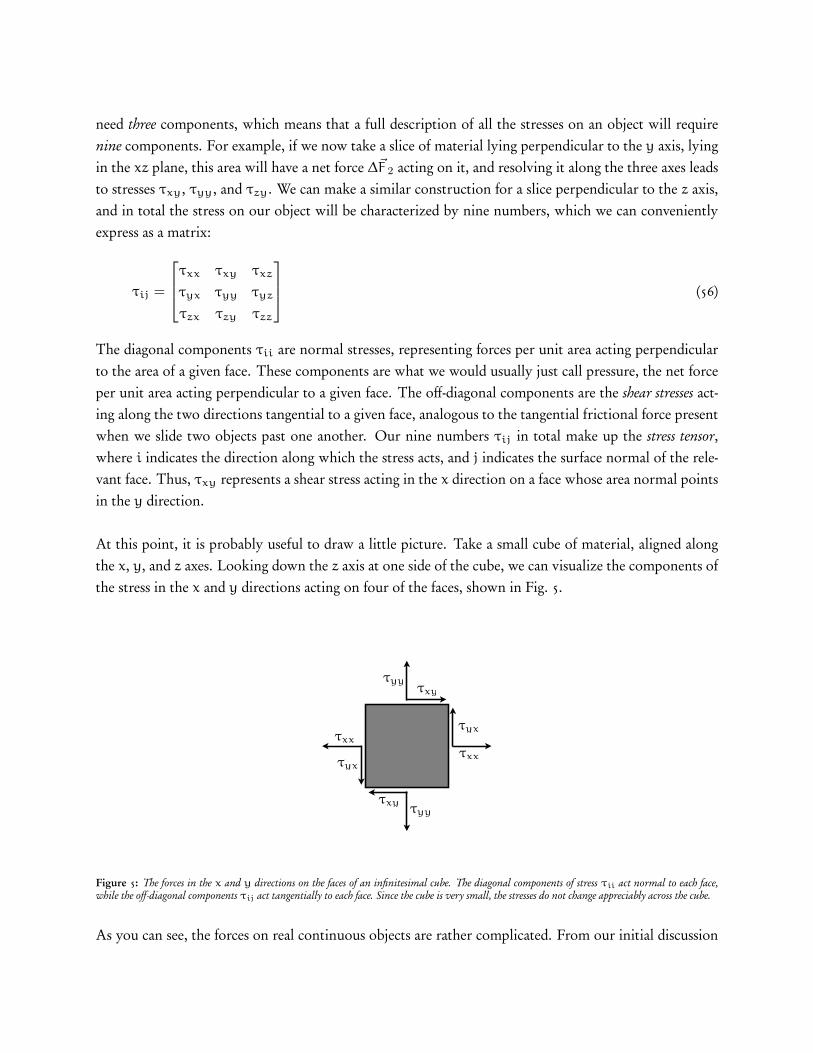
At this point, it is probably useful to draw a little picture. Take a small cube of material, aligned alongthe x, y, and z axes. Looking down the z axis at one side of the cube, we can visualize the components ofthe stress in the x and y directions acting on four of the faces, shown in Fig. 5.

τxx

τxxτyx

τyx

τyy

τyyτxy

τxy

Figure 5: The forces in the x and y directions on the faces of an infinitesimal cube. The diagonal components of stress τii act normal to each face,while the off-diagonal components τij act tangentially to each face. Since the cube is very small, the stresses do not change appreciably across the cube.

As you can see, the forces on real continuous objects are rather complicated. From our initial discussion

of a static fluid, requiring only a simple scalar pressure, we now have a nine-component second-ranktensor. However, it is not as bad as it seems: the stress tensor turns out to be symmetric, and we don’tneed all nine components. If we consider an infinitesimally small cube of material, then we can imaginethat the stresses do not change appreciable from one side to the other. As shown in the figure above, theforces on opposing sides of the cube must be equal and opposite in this case. This also implies that thetorque about the center of the cube is zero – if it were not, the cube would start spinning, which would beunphysical for an infinitesimally small object. If our cube has sides of dimension ∆a, then we can easilywrite down the torque about the center as ∆a(τyx − τxy) = 0, which means τxy = τyx. We can applythe same logic looking at the other faces of the cube, and just by considering that the cube must be inrotational equilibrium we find that the stress tensor must be symmetric, τij =τji. In short, we have onlyhave six unique components of stress, rather than nine.

Since our stress tensor is symmetric, it can be described by a symmetric matrix. If you have taken linearalgebra, you might recall that this leads us to an even more important property of the stress tensor: sinceit is symmetric, it is always possible to find a choice of coordinate axes for which it is diagonal. Thatis, if we choose our coordinate axes carefully, it is always possible to find a special orientation for whichour stress tensor has only the three components τxx, τyy, and τzz. In a perfect crystalline material,this special choice may correspond to the crystallographic axes, for instance. However, in general, thestress tensor varies from point to point in a material, meaning it is actually a tensor field. Just like wehave a scalar field T(x,y, z) describing the temperature everywhere in a room, or a vector field ~E (x,y, z)describing the electric field through all space, our stress tensor field describes the components of stressat all points in a material. At every point in space, the stress tensor gives us nine numbers – six uniquenumbers – describing the forces at that point, and thus a full description of the forces in a body requiresix functions of position.

6.1 The Maxwell stress tensor

Incidentally, there is a stress tensor associated with electromagetic forces per unit volume, the Maxwell stresstensor. The electromagnetic force per unit volume can be written in terms of the electric and magneticfields along with the charge and current densities

~f = ρ~E +~j × ~B (57)

Though it is quite some work to prove it, one can also write the electromagnetic force per unit volumeas the divergence of a second-rank tensor:

~f = ∇ · T (58)

Here T is the Maxwell stress tensor, and it is defined by

Tij = εo

(EiEj −

12δijE

2

)+

1µo

(BiBj −

12δijB

2

)(59)

Where δij is the Kronecker delta function, something which shows up quite a bit in tensor and vectoranalysis. It has a very simple definition:

δij =

0 i 6= j

1 i = j(60)

As with our general stress tensor in the previous section, the Tii components give rise to pressure-likeforces, while the Tij give rise to shear forces. You are certain to encounter this tensor again in laterphysics courses . . .

7 Viscosity and stress in three dimensions

After a long detour, we can finally return to our parallel plates moving within a fluid from Sect. 4. Recallour setup:

d

v = 0

v

Fvo

Figure 6: Viscous drag between two parallel plates in a fluid.

To be a bit more concrete, let the x axis be in the direction of the applied force, the y direction upward,and the z direction out of the page. Using our new tensor machinery, we can write the force per unitarea along the x direction required to keep the top plate moving as a stress:

τyx =Fx

∆y∆z= η

vo

d(61)

Thus, what we have previously considered is a shear stress acting tangential to the plates due to a viscous

force along the x axis, and empirically it is found to be proportional to the speed of the upper platethrough a scalar coefficient we call the viscosity.

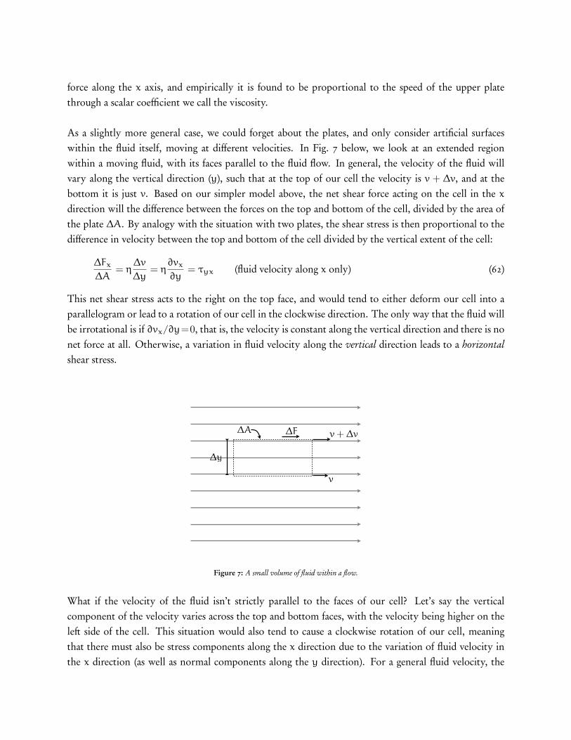
As a slightly more general case, we could forget about the plates, and only consider artificial surfaceswithin the fluid itself, moving at different velocities. In Fig. 7 below, we look at an extended regionwithin a moving fluid, with its faces parallel to the fluid flow. In general, the velocity of the fluid willvary along the vertical direction (y), such that at the top of our cell the velocity is v + ∆v, and at thebottom it is just v. Based on our simpler model above, the net shear force acting on the cell in the x

direction will the difference between the forces on the top and bottom of the cell, divided by the area ofthe plate ∆A. By analogy with the situation with two plates, the shear stress is then proportional to thedifference in velocity between the top and bottom of the cell divided by the vertical extent of the cell:

∆Fx

∆A= η

∆v

∆y= η

∂vx

∂y= τyx (fluid velocity along x only) (62)

This net shear stress acts to the right on the top face, and would tend to either deform our cell into aparallelogram or lead to a rotation of our cell in the clockwise direction. The only way that the fluid willbe irrotational is if ∂vx/∂y=0, that is, the velocity is constant along the vertical direction and there is nonet force at all. Otherwise, a variation in fluid velocity along the vertical direction leads to a horizontalshear stress.

∆y

∆A ∆F v + ∆v

v

Figure 7: A small volume of fluid within a flow.

What if the velocity of the fluid isn’t strictly parallel to the faces of our cell? Let’s say the verticalcomponent of the velocity varies across the top and bottom faces, with the velocity being higher on theleft side of the cell. This situation would also tend to cause a clockwise rotation of our cell, meaningthat there must also be stress components along the x direction due to the variation of fluid velocity inthe x direction (as well as normal components along the y direction). For a general fluid velocity, the

horizontal shear stress must then have two components:

τyx = η∂vy

∂x+ η

∂vx

∂y(63)

We could find the other shear components τyz and τzx similarly. Note that this equation immediatelysatisfies our symmetry requirement τxy = τyx. We can also see from this general expression that thereare only three cases in which there is no shear stress in the fluid: either the fluid is static (~v =0, the fluid’svelocity varies only along the out-of-plane z direction (∂vx/∂y=∂vy/∂x= 0), or the fluid is uniformlyrotating (∂vx/∂y=−∂vy/∂x). Of course, there are also no shear forces in a fluid with zero viscosity, butsuch things are incredibly rare.vii

Along these same lines, we can also find the normal stresses, those acting perpendicularly to the faces ofour cell. For example, if there is a variation in velocity along the vertical direction, then there will alsobe a net force on the cell in the vertical direction, along with the shear component:

τyy = 2η∂vx

∂x(64)

The normal components of the stress, τii, are what we would simply call pressure if the fluid were static.In the case of a moving fluid, the total normal force per unit area would be the static pressure P plus thenormal stress due to the fluid motion.

In general, so long as the fluid is incompressible, based on our description above you should be able toconvince yourself that the stress components are given by

τij = η

(∂vi

∂xj+

∂vj

∂xi

)(65)

8 Viscous forces in three dimensions

Now that we have the shear stresses in the fluid in the presence of viscosity, we can complete our equationof motion. All we need to do is work backwards to determine the forces on an arbitrary cell within amoving fluid from the stress components. Imagine we have again a small cube of fluid, Fig. 8, whose facesare aligned with our coordinate axes, with sides of length ∆x, ∆y, and ∆z. In addition to any hydrostaticpressure, our cube will have a force on each of its six sides due to the stress in the moving fluid fluid,whose velocity we will assume to vary in magnitude and direction.

First, we can tabulate all of the forces along a given axis, starting with x. All six faces of the cube willhave a stress component in the x direction: four shear forces, and two normal forces. On face 1, we have

viiLiquid helium is a so-called “superfluid” with zero viscosity, a macroscopic quantum-mechanical effect that can be observedonly at very low temperatures.

τxx

τxxτyx

τyx

τyy

τyyτxy

τxy

x x + ∆x

y

y + ∆y

12

3

4

Figure 8: The stresses in the x and y directions on the faces of a cube cube of fluid.

a normal stress component τxx acting over an area ∆y∆z, and net x component of the force on face 1will be the product of stress and area. However, we must be careful: the stress is really a tensor field, andit varies with position, so the value of τxx is different for face 1 and face 2, for instance. Thus, we shouldexplicitly note at which position we are evaluating the stress components. With that in mind,

Fx1 = τxx

∣∣∣∣x+∆x

∆y∆z (66)

The x component force on face two will be similar and opposite in sign, the only substantial difference isthat we are evaluating the stress tensor at a different position:

Fx2 = −τxx

∣∣∣∣∆x

∆y∆z (67)

Faces 3 and 4 will also have forces in the x direction through the shear stress τxy. Face 3 has area ∆x∆z

and it is located at vertical position y + ∆y. Face 4 has the same area, but the force is in the oppositedirection and τxy should be evaluated at a vertical position y.

Fx3 = τxy

∣∣∣∣y+∆y

∆x∆z (68)

Fx4 = −τxy

∣∣∣∣y

∆x∆z (69)

(70)

Finally, faces 5 and 6 (on the front and back of the cube in Fig. 8) also have forces along the x direction

through the shear stress τxy:

Fx5 = τxz

∣∣∣∣z+∆z

∆x∆y (71)

Fx6 = −τxz

∣∣∣∣z

∆x∆y (72)

(73)

All that is required now is to tabulate the net force along the x direction for the whole cube:

Fx = Fx1 + Fx2 + Fx3 + Fx4 + Fx5 + Fx6 (74)

=

(τxx

∣∣∣∣x+∆x

−τxx

∣∣∣∣x

)∆y∆z +

(τxy

∣∣∣∣y+∆y

−τxy

∣∣∣∣y

)∆x∆z +

(τxz

∣∣∣∣z+∆z

−τxz

∣∣∣∣z

)∆x∆y

(75)

= ∆τxx∆x∆z + ∆τxz∆x∆z + ∆τxz∆x∆y (76)

As with our equation of motion without viscosity, it is more useful to consider the force per unit volumealong x, which we’ll call fx:

fx =Fx

∆x∆y∆z=

∆τxx

∆x+

∆τxy

∆y+

∆τxz

∆z(77)

If we take the limit that the dimensions of our cube become infinitesimally small, what we have is thedefinition of a partial derivative:

fx =∂τxx

∂x+

∂τxy

∂y+

∂τxz

∂z(78)

We can repeat the analysis for the forces along the other directions, and our general expression for anincompressible fluid is

fi =

3∑j=1

∂τij

∂xjwith τij = η

(∂vi

∂xj+

∂vj

∂xi

)(79)

The stresses in a fluid depend on the velocity gradients in the fluid (or, equivalently, the rate of change ofshear strain), while the forces depend on the stress gradients. There will only be a net force on a volumeof fluid if there is a net spatial variation of stress, and there will only be stress if there is a net spatialvariation in velocity. Combining the two relationships above, we can cut out the middleman and relate

the viscous force per unit volume directly to the velocity distribution:

fi = η

3∑j=1

∂

∂xj

[∂vi

∂xj+

∂vj

∂xi

](80)

If we write out all three components of the force and rearrange the terms, we can recover a much morecompact vector equation. Let’s rearrange the sum and see what comes out:

fi = η

3∑j=1

∂

∂xj

[∂vi

∂xj+

∂vj

∂xi

]= η

3∑j=1

∂2vi

∂x2j

+ η∂

∂xi

3∑j=1

∂vj

∂xj= η∇2vi + η

∂

∂xi∇ · ~v (81)

Considering all three components of the force per unit volume, we have a nice vector equation in theend:

~f = η∇2~v + η∇ (∇ · ~v ) (82)

Here we have used the vector Laplacian∇2~v , which is just∇2vxx +∇2vyy +∇2vzz. We can make thisstill simpler, however, by remembering that for an incompressible fluid, the continuity equation reads∇ · ~v = 0. With that in mind, after much pain we ultimately have a simple form for the viscous force inan incompressible fluid

~f v = η∇2~v (viscous force, incompressible fluid) (83)

Our pervasive assumption of an incompressible fluid does come at a price. For instance, we will not beable to treat density variations in the fluid, such as sound waves. However, a wide variety of interestingfluids are essentially incompressible, and the form of the viscous force per unit volume above is sufficient.This assumption serves quite well for, e.g., air flowing at low speeds compared to the speed of sound.

9 The equation of motion with viscosity for incompressible fluids

The general equation of motion we developed was

ρ (~v · ∇) ~v + ρ∂~v

∂t= −∇P − ρ∇φ + ~f v (84)

where fv was our yet-to-be-determined viscous force. For an incompressible fluid, using the form of theviscous force from Eq. 83, our equation of motion reads

ρ (~v · ∇) ~v + ρ∂~v

∂t= −∇P − ρ∇φ + η∇2~v (85)

This non-linear partial differential equation is the Navier-Stokes equation for flow of Newtonian incom-pressible fluids. The Navier-Stokes equation is not straightforward to interpret qualitatively, and famously

difficult to solve in even the simplest cases. Another more common form substitutes the potential perunit mass ∇φ=−~g :

ρ

(∂~v

∂t+ ~v · ∇~v

)= −∇P + ρ~g + η∇2~v (86)

This form is more easily interpreted as a statement of Newton’s law: mass (ρ) times acceleration equalsthe sum of forces, namely pressure (−∇P), viscous forces (η∇2~v ), and gravity (ρ~g ). Since we are as-suming constant density (incompressible fluid), the continuity equation is simply ∇ · ~v = 0, which is astatement of conservation of fluid volume.

Incidentally, we can also reintroduce our vorticity ~Ω =∇× ~v :

ρ

(∂ρ

∂t+ ~Ω × ~v +

12∇v2

)= −∇P + ρ~g + η∇2~v (87)

That means that for an irrotational fluid ( ~Ω =0), we have

ρ

(∂ρ

∂t+

12∇v2

)= −∇P + ρ~g + η∇2~v (88)

The steady-state (∂ρ/∂t=0) equation for an irrotational fluid reads

12ρ∇v2 = −∇P + ρ~g + η∇2~v (89)

9.1 Steady flow through a long cylindrical pipe

Certainly after all this mess we should be able to handle the steady flow of water through a pipe. Let’stry it out. We will take a very long circular pipe of length L and radius R whose axis is oriented along thez direction, and it is carrying an incompressible fluid of density ρ. Clearly, it will be convenient to workin cylindrical coordinates. We will imagine that we set up a pressure difference between the end points toestablish a flow of fluid, such that we have a pressure PL at z=L and Po at z=0. If the pipe is very longand we can ignore the entrance and exit effects, then the pressure gradient along the length of the pipe isjust

∂P

∂z=

PL − Po

L(90)

Along the radial direction, there must be no pressure gradient if we have uniform flow of an incompress-ible fluid, ∂P/∂r=0. We can also establish some symmetry and boundary conditions on the velocity ofthe fluid in the pipe. Due to the symmetry of the problem, the velocity is independent of θ. Further,if the pipe is very long, then the radial component of the velocity vr should be independent of z (infact, it should be zero!). We need only worry about the variation of vz with r, since vz should also be

independent of z for a very long pipe – for an incompressible fluid, continuity ensures that the velocityof the fluid cannot vary along the length of the pipe. Finally, at the pipe boundary, we can also enforcethe prior condition that the fluid is static, such that v(R)=0. This condition means that the vz must peakat the center of the pipe, since it is zero at both edges, and thus ∂vz/∂r must vanish at the center of thepipe, r=0. The problem that remains is to deduce what the variation of velocity along the axis of the pipe.

If we are only interested in slow and steady flow through the pipe (small Reynolds’ numbers) of anincompressible fluid, we may also neglect the “acceleration” term in the Navier-Stokes equation 1

2ρ∇v2:

−∇P + η∇2~v + ρ~g = 0 (91)

This is just one step up from our equation of state for a completely static fluid, we now retain only theviscous force η∇2~v . Neglecting the acceleration is just saying we wish to find a solution for which thevelocity is constant, the definition of steady flow. Since we may also neglect the variation of velocitiesalong the θ direction, in cylindrical coordinates we have a simplified Navier-Stokes equation:

−∂P

∂r+ η

[∂

∂r

(1r

∂

∂r(rvr)

)+

∂2vr

∂z2

]+ ρgr = 0 (92)

−∂P

∂z+ η

[1r

∂

∂r

(r∂vz

∂r

)+

∂2vz

∂z2

]+ ρgz = 0 (93)

If we assume that the gravitational force acts along the −z direction only and apply our boundary/symmetryconditions, we have

η

[∂

∂r

(1r

∂

∂r(rvr)

)]= 0 (94)

η

[1r

∂

∂r

(r∂vz

∂r

)]+ ρgz =

PL − Po

L(95)

If we rearrange the second equation,

1r

∂

∂r

(r∂vz

∂r

)=

1η

(PL − Po

L− ρgz

)(96)

Multiplying both sides by r and integrating with respect to r, we have

r∂vz

∂r=

r2

2η

(PL − Po

L− ρgz

)+ Co (97)

where Co is a constant of integration, to be determined by the boundary conditions. We can pull thesame trick twice, this time dividing by r and integrating with respect to r, and arrive at

vz =r2

4η

(PL − Po

L− ρgz

)+ Cor + C1 (98)

where C1 is a second constant of integration. We can eliminate Co by enforcing the condition that at thecenter of the pipe, r=0, ∂vz/∂r must vanish. We can find C1 by enforcing the condition that vz(R)=0:

vz(R) = 0 =R2

4η

(PL − Po

L− ρgz

)+ C1 =⇒ C1 =

R2

4η

(Po − PL

L− ρgz

)(99)

This fully determines the radial variation of the vertical velocity of the fluid in the pipe:

vz(r) =

(Po − PL

4ηL

)(R2 − r2

)(100)

Given this distribution, we could find the volumetric flow rate Q (e.g., cubic meters per second) by firstfinding the average velocity over the cross-sectional area of the pipe, and multiplying by the area:

vz =1

πR2

2π∫0

R∫0

vzr dr dθ =

[Po − PL

L+ ρgz

]R2

8η(101)

Q = πR2vz

[Po − PL

L+ ρgz

]πR4

8η(102)

This is the famous Hager-Poiseuille law, and the basis for most plumbing you will encounter.

9.2 Stoke’s flow around a solid sphere

Now let us consider the steady flow of an incompressible fluid around a dense, solid sphere, or equiva-lently, a solid sphere falling in a static fluid. For small spheres, this leads to measurement known as thefalling sphere viscometer, as we will find that the terminal velocity of the falling sphere will be inverselyproportional to the viscosity. As in the example above, in this case we may neglect the “acceleration”term in the Navier-Stokes equation 1

2ρ∇v2:

−∇P + η∇2~v + ρ~g = 0 (103)

Further simplification is possible in this case due to the symmetry of the problem. Let the fluid flow bealong the z axis with constant velocity V∞, with the solid sphere of radius R at the origin. In this case,by symmetry the fluid momentum is clearly independent of ϕ (the angle in the xy plane). In sphericalcoordinates the Navier-Stokes and continuity equations read

−∂P

∂r+ η

[∇2vr −

2vr

r2−

2r2

∂vθ

∂θ−

2r2

vθ cot θ

]+ ρgr = 0 (104)

−1r

∂P

∂θ+ η

[∇2vθ +

2r2

∂vr

∂θ−

vθ

r2 sin2 θ

]+ ρgθ = 0 (105)

1r2

∂

∂r

(r2vr

)+

1r sin θ

∂

∂θ(vθ sin θ) = 0 (106)

Here we have expanded the θ and r portions of the gradient operators in spherical coordinates. Per-haps surprisingly, the stress distribution, pressure distribution, and velocity components can be foundanalytically:

τrθ =32

ηV∞R

(R

r

)4

sin θ (107)

P = Po − ρgz −32

ηV∞R

(R

r

)2

cos θ (108)

vr = V∞(

1 −32

(R

r

)+

12

(R

r

)3)

cos θ (109)

vθ = −V∞(

1 −34

(R

r

)−

14

(R

r

)3)

sin θ (110)

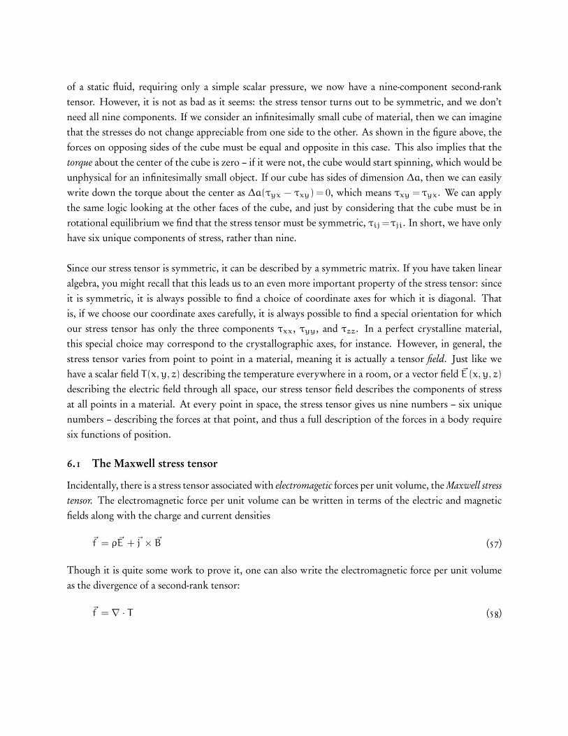
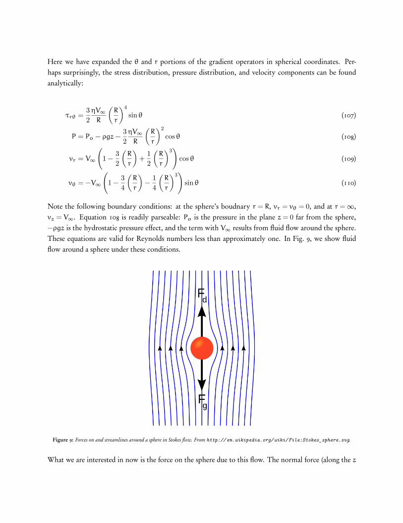
Note the following boundary conditions: at the sphere’s boudnary r = R, vr = vθ = 0, and at r = ∞,vz = V∞. Equation 108 is readily parseable: Po is the pressure in the plane z = 0 far from the sphere,−ρgz is the hydrostatic pressure effect, and the term with V∞ results from fluid flow around the sphere.These equations are valid for Reynolds numbers less than approximately one. In Fig. 9, we show fluidflow around a sphere under these conditions.

Figure 9: Forces on and streamlines around a sphere in Stokes flow. From http://en.wikipedia.org/wiki/File:Stokes_sphere.svg.

What we are interested in now is the force on the sphere due to this flow. The normal force (along the z

axis) acting on the solid sphere is due to the pressure given by Eq. 108 with r=R and z=R cos θ:

P(r = R) = Po − ρgR cos θ −32

ηV∞R

cos θ (111)

The net upward force in the z direction due to the pressure difference on the ‘top’ and ‘bottom’ portionsof the sphere is found by multiplying this pressure times the infinitesimal bit of surface area over whichit acts, R2 sin θdθ dϕ and integrating over the surface of the sphere:

Fn =

2π∫0

π∫0

[Po − ρgR cos θ −

32

ηV∞R

cos θ

]R2 sin θdθ dϕ (112)

Fn =43πR3ρg + 2πηRV∞ (113)

We recover two terms for the normal force: the first is the buoyant force and the second the form drag. Ateach point on the surface, there is also a shear stress acting tangentially, −τrθ. This tangential force, sincewe are dealing with a curved surface, has both x−y and z components. Over the whole sphere, the formerwill vanish by symmetry, but the latter will give rise to a net force for any non-zero fluid velocity. On anyinfinitesimal patch of surface, the z-component of this tangential force is (−τrθ) (− sin θ) R2 sin θdθ dϕ,and once again integrating over the sphere’s surface we find

Ft =

2π∫0

π∫0

(τrθ|r=R sin θ) R2 sin θ dθdϕ (114)

From Eq 107,

τrθ

∣∣∣∣r=R

=32

ηV∞R

sin θ (115)

which results in a net frictional drag from the tangential flow of

Ft = 4πηRV∞ (116)

Thus, the total force on our sphere in the flowing fluid is

F =43πR3ρg + 6πηRV∞ (117)

The force has two terms, as expected: the first due to gravity (the weight of the fluid), exerted even ifthe fluid is stationary, and the second associated with fluid motion, sometimes called the “drag force.”Both forces act in the same direction, opposing the direction of fluid flow. Sometimes, you will see the

quantity 6πηR=b called the “Stokes radius,” leading to a nice form of the force equation:

F =43πR3ρg + bV∞ =

mspheregρ

ρsphere+ bV∞ (118)

Equation 117 is known as Stoke’s law, and from it we may determine the terminal velocity of a fallingsphere. Consider a sphere falling in a stagnant fluid of density ρs. In this case V∞ is the relative velocityof the fluid with respect to the sphere, which in this case is just the velocity of the falling sphere since thefluid is stationary. The static and drag Stoke’s forces act opposite the direction that the sphere falls, andat the terminal velocity Vt, precisely balance the sphere’s weight. If the sphere has density ρs, this means

43πR3ρg + 6πηRVt =

43πR3ρsg (119)

This leads to a terminal velocity of

Vt =2gR2 (ρs − ρ)

9η(120)

As expected, it is the relative density of fluid and solid that determine the behavior of the sphere: if thesphere is more dense than the fluid, it sinks, and if it is less dense than the fluid, it rises. If the particleradius and densities are known, a velocity measurement allows one to deduce the viscosity of a fluid.Conversely, if the densities and viscosity are known, one can find the radius of a small particle. Thelatter is useful in so-called fluidized bed particle separators, allowing one to separate particles by their sizedistribution.