a course on elementary probability theory - arxiv · gane samb lo a course on elementary...
TRANSCRIPT

Gane Samb LO
A Course on ElementaryProbability Theory
Statistics and Probability African Society(SPAS) Books Series.
Saint-Louis, Calgary, Alberta. 2016.
DOI : http://dx.doi.org/10.16929/sbs/2016.0003
ISBN 978-2-9559183-3-3
i
arX
iv:1
703.
0964
8v3
[m
ath.
HO
] 1
4 M
ay 2
018

ii
SPAS TEXTBOOKS SERIES
GENERAL EDITOR of SPAS EDITIONS
Prof Gane Samb [email protected], [email protected] Berger University (UGB), Saint-Louis, SENEGAL.African University of Sciences and Technology, AUST, Abuja, Nigeria.
ASSOCIATED EDITORS
KEHINDE DAHUD [email protected] Of BOTSWANA
Blaise [email protected] of LANIBIO, UFR/SEAOuaga I Pr Joseph Ki-Zerbo University.
ADVISORS
Ahmadou Bamba [email protected] Berger University, Senegal.
Tchilabalo Abozou [email protected] University, Togo.

iii
List of published books
SPAS Textbooks Series.
Weak Convergence (IA). Sequences of random vectors.Par Gane Samb LO, Modou Ngom and Tchilabalo Abozou KPANZOU.(2016) Doi : 10.16929/sbs/2016.0001. ISBN : 978-2-9559183-1-9 (Eng-lish).
A Course on Elementary Probability Theory.Gane Samb LO (March 2017)Doi : 10.16929/sbs/2016.0003. ISBN : 978-2-9559183-3-3 (English).
For the latest updates, visit our official website :
www.statpas.net/spaseds/

iv
Library of Congress Cataloging-in-Publication Data
Gane Samb LO, 1958-
A Course on Elementary Probability Theory.
SPAS Books Series, 2016.
Copyright c©Statistics and Probability African Society (SPAS).
DOI : 10.16929/sbs/2016.0003
ISBN 978-2-9559183-3-3

v
Author : Gane Samb LO
Emails:[email protected], [email protected], [email protected]
Url’s:[email protected]/[email protected].
Affiliations.Main affiliation : University Gaston Berger, UGB, SENEGAL.African University of Sciences and Technology, AUST, ABuja, Nigeria.Affiliated as a researcher to : LSTA, Pierre et Marie Curie University,Paris VI, France.
Teaches or has taught at the graduate level in the following univer-sities:Saint-Louis, Senegal (UGB)Banjul, Gambia (TUG)Bamako, Mali (USTTB)Ouagadougou - Burkina Faso (UJK)African Institute of Mathematical Sciences, Mbour, SENEGAL, AIMS.Franceville, Gabon
Acknowledgment of Funding.
The author acknowledges continuous support of the World Bank Ex-cellence Center in Mathematics, Computer Sciences and IntelligenceTechnology, CEA-MITIC. His research projects in 2014, 2015 and 2016are funded by the University of Gaston Berger in different forms andby CEA-MITIC.


A Course on Elementary Probability Theory

ix
Abstract. (English) This book introduces to the theory ofprobabilities from the beginning. Assuming that the readerpossesses the normal mathematical level acquired at the endof the secondary school, we aim to equip him with a solid ba-sis in probability theory. The theory is preceded by a generalchapter on counting methods. Then, the theory of probabili-ties is presented in a discrete framework. Two objectives aresought. The first is to give the reader the ability to solve alarge number of problems related to probability theory, in-cluding application problems in a variety of disciplines. Thesecond was to prepare the reader before he approached themanual on the mathematical foundations of probability the-ory. In this book, the reader will concentrate more on math-ematical concepts, while in the present text, experimentalframeworks are mostly found. If both objectives are met,the reader will have already acquired a definitive experiencein problem-solving ability with the tools of probability theoryand at the same time he is ready to move on to a theoreticalcourse on probability theory based on the theory of measure-ment and integration. The book ends with a chapter thatallows the reader to begin an intermediate course in mathe-matical statistics.
(Francais) Cet ouvrage introduit a la theorie des proba-bilites depuis le debut. En supposant que le lecteur possedele niveau mathematique normal acquis a la fin du lycee,nous ambitionnons de le doter d’une base solide en theoriedes probabilites. L’expose de la theorie est precede d’unchapitre general sur les methodes de comptage. Ensuite, latheorie des probabilites est presentee dans un cadre discret.Deux objectifs sont recherches. Le premier est de donner aulecteur la capacite a resoudre un grand nombre de problemeslies a la theorie des probabilites, y compris les problemesd’application dans une variete de disciplines. Le second etaitde preparer le lecteur avant qu’il n’aborde l’ouvrage sur lesfondements mathematiques de la theorie des probabilites.Dans ce dernier ouvrage, le lecteur se concentrera davantagesur des concepts mathematiques tandis que dans le presenttexte, il se trouvent surtout des cadres experimentaux. Si lesdeux objectifs sont atteints, le lecteur aura deja acquis uneexperience definitive en capacite de resolution de problemesde la vie reelle avec les outils de la theorie des probabiliteset en mme temps, il est prt a passer a un cours theoriquesur les probabilites basees sur la theorie de la mesure etl’integration. Le livre se termine par par un chapitre quipermet au lecteur de commencer un cours intermediaire enstatistiques mathematiques.

x
Keywords. Combinatorics; Discrete counting; Elementary Probabil-ity; Equi-probability; Events and operation on events; Independence ofevents; Conditional probabilities; Bayes’ rules; Random variables; Dis-crete and continuous random variables; Probability laws; Probabilitydensity functions; Cumulative distribution functions; Independence ofrandom variables; Usual probability laws and their parameters; intro-duction to statistical mathematics.
AMS 2010 Classification Subjects : 60GXX; 62GXX.

Contents
General Preface 3
Preface of the first edition 2016 5
Introduction 91. The point of view of Probability Theory 92. The point of view of Statistics 103. Comparison between the two approaches 114. Brief presentation of the book 12
Chapter 1. Elements of Combinatorics 151. General Counting principle 152. Arrangements and permutations 163. Number of Injections, Number of Applications 184. Permutations 195. Permutations with repetition 206. Stirling’s Formula 30
Chapter 2. Introduction to Probability Measures 311. An introductory example 312. Discrete Probability Measures 333. equi-probability 38
Chapter 3. Conditional Probability and Independence 411. The notion of conditional probability 412. Bayes Formula 443. Independence 50
Chapter 4. Random Variables 551. Introduction 552. Probability Distributions of Random Variables 583. Probability laws of Usual Random Variables 604. Independence of random variables 70
Chapter 5. Real-valued Random Variable Parameters 731. Mean and Mathematical Expectation 73
i

ii CONTENTS
2. Definition and examples 743. General Properties of the Mathematical Expectation 754. Usual Parameters of Real-valued Random Variables 825. Parameters of Usual Probability law 946. Importance of the mean and the standard deviation 100
Chapter 6. Random couples 1051. Strict and Extended Values Set for a Discrete Random
Variable 1052. Joint Probability Law and Marginal Probability Laws 1073. Independence 1104. An introduction to Conditional Probability and Expectation127
Chapter 7. Continuous Random Variables 1351. Cumulative Distribution Functions of a Real-valued random
Variable (rrv) 1352. General properties of cdf ’s 1393. Real Cumulative Distribution Functions on R 1414. Absolutely Continuous Distribution Functions 1445. The origins of the Gaussian law in the earlier Works of de
Moivre and Laplace (1732 - 1801) 1516. Numerical Probabilities 160
Chapter 8. Appendix : Elements of Calculus 1651. Review on limits in R. What should not be ignored on
limits. 1652. Convex functions 1773. Monotone Convergence and Dominated Converges of series 1824. Proof of Stirling’s Formula 189
Bibliography 197

CONTENTS 1
Dedication.
To our beloved and late sister Khady Kane LO27/07/1953 - 7/11/1988
Figure 1. The ever smiling young lady


General Preface
This textbook part of a series whose ambition is to cover broad partof Probability Theory and Statistics. These textbooks are intended tohelp learners and readers, both of of all levels, to train themselves.
As well, they may constitute helpful documents for professors andteachers for both courses and exercises. For more ambitious people,they are only starting points towards more advanced and personalizedbooks. So, these texts are kindly put at the disposal of professors andlearners.
Our textbooks are classified into categories.
A series of introductory books for beginners. Books of this seriesare usually accessible to student of first year in universities. They donot require advanced mathematics. Books on elementary probabilitytheory and descriptive statistics are to be put in that category. Booksof that kind are usually introductions to more advanced and mathe-matical versions of the same theory. The first prepare the applicationsof the second.
A series of books oriented to applications. Students or researchersin very related disciplines such as Health studies, Hydrology, Finance,Economics, etc. may be in need of Probability Theory or Statistics.They are not interested by these disciplines by themselves. Rather, theneed to apply their findings as tools to solve their specific problems. Soadapted books on Probability Theory and Statistics may be composedto on the applications of such fields. A perfect example concerns theneed of mathematical statistics for economists who do not necessarilyhave a good background in Measure Theory.
A series of specialized books on Probability theory and Sta-tistics of high level. This series begin with a book on Measure The-ory, its counterpart of probability theory, and an introductory book ontopology. On that basis, we will have, as much as possible, a coherent
3

4 GENERAL PREFACE
presentation of branches of Probability theory and Statistics. We willtry to have a self-contained, as much as possible, so that anything weneed will be in the series.
Finally, research monographs close this architecture. The archi-tecture should be so large and deep that the readers of monographsbooklets will find all needed theories and inputs in it.
We conclude by saying that, with only an undergraduate level, thereader will open the door of anything in Probability theory and sta-tistics with Measure Theory and integration. Once this coursevalidated, eventually combined with two solid courses on topology andfunctional analysis, he will have all the means to get specialized in anybranch in these disciplines.
Our collaborators and former students are invited to make live thistrend and to develop it so that the center of Saint-Louis becomes orcontinues to be a re-known mathematical school, especially in Proba-bility Theory and Statistics.

Preface of the first edition 2016
The current series of Probability Theory and Statistics are basedon two introductory books for beginners : A Course of Elementaryprobability Theory and A course on Descriptive Statistics.
All the more or less advanced probability courses are preceded by thisone. We strongly recommend to not skip it. It has the tremendousadvantage to make feel the reader the essence of probability theoryby using extensively random experiences. The mathematical conceptscome only after a complete description of a random experience.
This book introduces to the theory of probabilities from the beginning.Assuming that the reader possesses the normal mathematical level ac-quired at the end of the secondary school, we aim to equip him with asolid basis in probability theory. The theory is preceded by a generalchapter on counting methods. Then, the theory of probabilities is pre-sented in a discrete framework.
Two objectives are sought. The first is to give the reader the ability tosolve a large number of problems related to probability theory, includ-ing application problems in a variety of disciplines. The second wasto prepare the reader before he approached the textbook on the math-ematical foundations of probability theory. In this book, the readerwill concentrate more on mathematical concepts, while in the presenttext, experimental frameworks are mostly found. If both objectivesare met, the reader will have already acquired a definitive experiencein problem-solving ability with the tools of probability theory and atthe same time he is ready to move on to a theoretical course on prob-ability theory based on the theory of measurement and integration.
The book ends with a chapter that allows the reader to begin an inter-mediate course in mathematical statistics.I wish you a pleasant reading and hope receiving your feedback.
5

6 PREFACE OF THE FIRST EDITION 2016
To my late and beloved sister Khady Kane Lo(1953- ).
Saint-Louis, Calgary, Abuja, Bamako, Ouagadougou, 2017.
PREFACE OF THE FIRST EDITION 2016 7
Preliminary Remarks and Notations.
WARNINGS
(1)
(2)

Introduction
There exists a tremendous number of random phenomena in nature,real life and experimental sciences.
Almost everything is random in nature : whether, occurrences of rainand their durations, number of double stars in a region of the sky, life-times of plants, of humans, and of animals, life span of a radioactiveatom, phenotypes of offspring of plants or any biological beings, etc.
The general theory states that each phenomena has a structural part(that is deterministic) and an random part (called the error or the de-viation).
Random also appears is conceptual experiments : tossing a coin onceor 100 times, throwing three dice, arranging a deck of cards, matchingtwo decks, playing roulettes, etc.
Every day human life is subject to random : waiting times for buses,traffic, number of calls on a telephone, number of busy lines in a com-munication network, sex of a newborn, etc.
The reader is referred to [Feller (1968)] for a more diverse and richset of examples.
The quantitative study of random phenomena is the objective of Prob-ability Theory and Statistics Theory. Let us give two simple examplesto briefly describe each of these two disciplines.
1. The point of view of Probability Theory
In Probability Theory, one assigns a chance of realization to a randomevent before its realization, taking into account the available informa-tion.
9

10 INTRODUCTION
Example : A good coin, that is a homogenous and well balanced, istossed. Knowing that the coin cannot stand on its rim, there is a 50%chances of having a Tail.
We base our conclusion on the lack of any reason to favor one of thepossible outcomes : head or tail. So we convene that these outcomesare equally probable and then get 50% chances for the occurring foreach of them.
2. The point of view of Statistics
Let us start with an example. Suppose that we have a coin and we donot know any thing of the material structure of the coin. In particular,we doubt that the coin is homogenous.
We decide to toss it repeatedly and to progressively monitor the oc-curring frequency of the head. We denote by Nn the number of headsobtained after n tossings and define the frequency of the heads by
Fn =Nn
n.
It is conceivable to say that the stability of Fn in the neighborhood ofsome value p ∈]0, 1[ is an important information about the structureof the coin.
In particular, if we observe that the frequency Fn does not deviate fromp = 50% more than ε = 0.001 whenever n is greater than 100, that is
|Fn − 1/2| ≤ 10−3.
for n ≥ 100, we will be keen to say that the probability of occurrenceof the head is p = 50% and, by this, we accept that that the coin is fair.
Based on the data (also called the statistics), we estimated the prob-ability of having a head at p = 50% and accepted the pre-conceivedidea (hypothesis) that the coin is good in the sense of homogeneity.
The reasoning we made and the method we applied are perfect illustra-tions of Statistical Methodology : estimation and model or hypothesisvalidation from data.

3. COMPARISON BETWEEN THE TWO APPROACHES 11
In conclusion, Statistics Theory enables the use of the data (alsocalled statistics or observations), to estimate the law of a random phe-nomenon and to use that law to predict the future of the same phe-nomenon (inference) or to predict any other phenomenon that seemsidentical to it (extrapolation).
3. Comparison between the two approaches
(1) The discipline of Statistics Theory and that of Probability Theoryare two ways of treating the same random problems.
(2) The first is based primarily on the data to draw conclusions .
(3) The second is based on theoretical, and mathematical considera-tions to establish theoretical formulas.
(4) Nevertheless, the Statistics discipline may be seen as the culmina-tion of Probability Theory.

12 INTRODUCTION
4. Brief presentation of the book
This book is an introduction to Elementary Probability Theory. It isthe result of many years of teaching the discipline in Universities andHigh schools, mainly in Gaston Berger Campus of Saint-Louis, SENE-GAL.
It is intended to those who have never done it before. It focuses on theessential points of the theory. It is particularly adapted for undergrad-uate students in the first year of high schools.
The basic idea of this book consists of introducing Probability Theory,and the notions of events and random variables in discrete probabilityspaces. In such spaces, we discover as much as possible at this level,the fundamental properties and tools of the theory.
So, we do not need at this stage the elaborated notion of σ-algebrasor fields. This useful and brilliant method has already been used, forinstance, in Billingsley [Billingsley (1995)] for deep and advancedprobability problems.
The book will finish by a bridge chapter towards a medium course ofMathematical Statistics. In this chapter, we use an anology methodto express the former results in a general shape, that will be the firstchapter of the afore mentioned course.
The reader will have the opportunity to master the tools he will be us-ing in this course, with the course on the mathematical foundation ofProbability Theory he will find in Lo [Lo (2016)], which is an elementof our Probability and Statistics series. But, as explained in the pref-aces, the reader will have to get prepared by a course of measure theory.
In this computer dominated world, we are lucky to have very powerfuland free softwares like R and Scilab, to cite only the most celebrated.We seized this tremendous opportunity to use numerical examples us-ing R software throughout the text.
The remainder of the book is organized as following.
Chapter 1 is a quick but sufficient introduction to combinatorial analy-sis. The student interested in furthering knowledge in this subject can

4. BRIEF PRESENTATION OF THE BOOK 13
refer to the course on general algebra.
Chapter 2 is devoted to an introduction to probability measures in dis-crete spaces. The notion of equi-probability is also dealt with, there.
Conditional probability and independence of random events are ad-dressed with in Chapter 3.
Chapter 4 introduces random variables, and presents a review of theusual probability laws.
Chapter 5 is devoted to the computations of the parameters of theusual laws. Mastering the results of this chapter and those in Chapter4 is in fact of great importance for higher level courses.
Distribution functions of random variables are studied in Chapter 7,which introduces non-discrete random variables.


CHAPTER 1
Elements of Combinatorics
Here, we are concerned with counting cardinalities of subsets ofa reference set Ω, by following specific rules. We begin by a generalcounting principle.
The cardinality of a set E is its number of elements, denoted byCard(E) or #(E). For an infinite set E, we have
Card(E) = #(E) = +∞.
1. General Counting principle
Let us consider the following example : A student has two (2) skirtsand four (4) pants in his closet. He decides to pick at random a skirtand a pant to dress. In how many ways can he dress by choosing askirt and a pant? Surely, he has 2 choices for choosing a skirt and foreach of these choices, he has four possibilities to pick a pant. In total,he has
2× 4
ways to dress.
We applied the following general counting principle.
Proposition 2.1. Suppose that the set Ω of size n can be partitionedinto n1 subsets Ωi, i = 1, ..., n1 of same size; and that each of these sub-sets Ωi can be split into n2 subsets Ωij, j = 1, . . ., n2, i = 1, ..., n1, ofsame size, and that each of the Ωij can be divided into n3 subsets Ωijh,h = 1, ..., n3, j = 1, ..., n2, i = 1, ..., n1 of same size also. Suppose thatwe may proceed like that up an order k with nk subsets with commonsize a.
Then the cardinality of Ω is given by
15

16 1. ELEMENTS OF COMBINATORICS
n = n1 × n2 ××...× nk × a
Proof. Denote by Bh the cardinality of a subset generated at step h,for h = 0, ..., k. A step h, we have nh subsets partitioned into nh+1
subsets of same size. Then we have
Bh = nh+1 ×Bh+1 for all 0 ≤ h ≤ k + 1.
with B0 = n, Bk+1 = a. Now, the proof is achieved by induction in thefollowing way
n = B0 = n1 ×B1
= n1 × n2 × n3B3
...
= n1 × n2 × n3B3 × ....× nk ×B(k + 1),
with B(k + 1) = a.
Although this principle is simple, it is a fundamental tool in combina-torics : divide and count.
But it is not always applied in a so simple form. Indeed, partitioningis the most important skill to develop in order to apply the principlesuccessfully.
This is what we will be doing in all this chapter.
2. Arrangements and permutations
Let E be a set of n elements with n ≥ 1.
Definition 2.1. A p-tuple of E is an ordered subset of E with p distinctelements of E. A p-tuple is called a p-permutation or p-arrangementof elements of E and the number of p-permutations of elements of Eis denoted as Apn (we read p before n). It as also denoted by (n)p.
We have the result.
Theorem 2.1. For all 1 ≤ p ≤ n, we have
Apn = n(n− 1)(n− 2)......(n− p+ 1).

2. ARRANGEMENTS AND PERMUTATIONS 17
Proof. Set E = x1, ..., xn. Let Ω be the class of all ordered subsetsof p elements of E. We are going to apply the counting principle to Ω.
It is clear that Ω may be divided into n = n1 subsets Fi, where eachFi is the class of ordered subsets of Ω with first elements xi. Since thefirst element is fixed to xi, the cardinality of Fi is the number orderedsubsets of E\xi, so that the classes Fi have a common cardinality whichis the number of (p − 1)-permutations from a set of (n − 1) elements.We have proved that
(2.1) Apn = n× Ap−1n−1,
for any 1 ≤ p ≤ n. We get by induction
Apn = n× (n− 1)× Ap−2n−2
and after h repetitions of (2.1), we arrive at
Apn = n× (n− 1)× (n− 2)× ...× (n− h)× Ap−hn−h.
For h = p− 2, we have
Apn = n× (n− 1)× (n− 2)× ...× (n− p+ 2)× A1n−p+1.
And, clearly, A1n−p+1 = n−p+1 since A1
n−p+1 is the number of singletonsform a set of (n− p+ 1) elements.
Remark. Needless to say, we have Apn = 0 for p ≤ n+ 1.
Here are some remarkable values of Apn. For any positive integer n ≥ 1,we have
(i) A0n = Ann = 1.
(ii) A1n = n.
From an algebraic point of view, the numbers Apn also count the numberof injections.

18 1. ELEMENTS OF COMBINATORICS
3. Number of Injections, Number of Applications
We begin to remind the following algebraic definitions :
A function from a set E to a set F is a correspondence from E to Fsuch that each element of E has at most one image in F .
An application from a set E to a set F is a correspondence from E toF such that each element of E has exactly one image in F .
An injection from a set E to a set F is an application from E to Fsuch that each any two distinct elements of E have distinct images in F .
A surjection from a set E to a set F is an application from E to Fsuch that each element of F is the image of at least one element of E.
A bijection from a set E onto a set F is an application from E to Fsuch that that each element of F is the image of one and only elementof E.
If there is an injection (respectively a bijection) from E to F , then wehave the inequality :Card(E) ≤ Card(F ) (respectively, the equalityCard(E) = Card(F )).
The number of p-arrangements from n elements (p ≤ n) is thenumber of injections from a set of p elements to a set of nelements.
The reason is the following. Let E = y1, ..., yp and F = x1, x2,..., xnbe sets with Card(E) = p and Card(F ) = n with p ≤ n. Forming aninjection f from E on F is equivalent to choosing a p-tuple (xi1 ...xip)in F and to set the following correspondance f(yh) = xih , h = 1, ..., p.So, we may find as many injections from E to F as p-permutations ofelements of from F .
Thus, Apn is also the number of injections from a set of p elements ona set of n elements.

4. PERMUTATIONS 19
The number of applications from a set of p elements to a setof n elements is np.
Indeed, let E = y1, ..., yp and F = x1, x2,..., xn be sets with Card(E) =p and Card(F ) = n with no relation between p and n. Forming an ap-plication f from E on F is equivalent to choosing, for any x ∈ E, onearbitrary element of F and to assign it to x as its image. For the firstelement x1 of E, we have n choices, n choices also for the second x2, nchoices also for the third x3, and so forth. In total, we have choices toform an application from E to F .
Example on votes casting in Elections. The p members of somepopulation are called to mandatory cast a vote for one of n candi-dates at random. The number of possible outcomes is the number ofinjections from a set of p elements to a set of n elements : np.
4. Permutations
Definition 2.2. A permutation or an ordering of the elements of E isany ordering of all its elements. If n is the cardinality of E, the numberof permutations of the element of E is called : n factorial, and denotedn! (that is n followed with an exclamation point).
Before we give the properties of n factorial, we point out that a per-mutation of n objects is a n-permutation of n elements.
Theorem 2.2. For any n ≥ 1, we have
(i) n! = n(n− 1)(n− 2)......2× 1.
(ii) n! = n(n− 1)!.
Proof. By reminding that a permutation of n objects is a n-permutationof n elements, we may see that Point (i) is obtained for p = n in theFormula of Theorem 2.1. Point (ii) obviously derives from from (i) byinduction.
Exercise 2.1. What is the number of bijections between two sets ofcommon cardinalily n ≥ 1?

20 1. ELEMENTS OF COMBINATORICS
Exercise 2.2. Check that for any pour 1 ≤ p ≤ n.
Apn = n!/(n− p)!,
5. Permutations with repetition
Let E be collection of n distinct objects. Suppose that E is par-titioned into k sub-collections Ej of respective sizes n1, . . .nk thefollowing properties apply :
(i) Two elements of a same sub-collection are indistinguishable betweenthem.
(ii) Two elements from two different sub-collections are distinguishableone from the other.
What is the number of permutations of E? Let us give an example.
Suppose we have n = 20 balls of the same form (not distinguishableby the form, not at sight nor by touch), with n1 = 6 of them in redcolor, n2 = 9 of blue color and n3 = 5 of green color. And we candistinguish them only by their colors. In this context, two balls of thesame color are the same for us, from our sight. An ordering of these nballs in which we cannot distinguish the balls of a same color is calleda permutation with repetition or a visible permutation.
Suppose that have we realized a permutation of these n balls. Per-muting for example only red balls between them does not change theappearance of the global permutation. Physically, it has changed butnot visibly meaning from our sight. Such a permutation may be de-scribed as visible, or permutation with repetition.
In fact, any of n! real permutations represents all the visible repetitionswhere the 6 red balls are permuted between them, the 9 blue balls arepermuted between them and the 5 green balls are permuted betweenthem. By the counting principle, a real permutation represents exactly
9!× 6!× 5!

5. PERMUTATIONS WITH REPETITION 21
permutations with repetition. Hence, the number of permutations withrepetition of these 20 balls is
20!
9!× 6!× 5!
Now, we are going to do the same reasoning in the general case.
As we said before, we have two types of permutations here :
(a) The real or physical permutations, where the n are supposed to bedistinguishable.
(b) The permutations with repetition in which we cannot distinguishbetween the elements of a same sub-collection.
Theorem 2.3. The number of permutations with repetition of a col-lection E of n objects partitioned into k sub-collections Ei of size ni,i = 1, ..., k, such such only elements from different sub-collections aredistinguishable between them, is given by
B(n1, n2, ..., nk) =n!
n1!n2!......nk!.
Terminology. The numbers of permutations with repetition are alsocalled multinomial coefficients, in reference Formula (5.3).
Proof. Let B(n1, n2, ..., nk) be number of permutations with repeti-tion. Consider a fixed real permutation. This real permutation cor-responds exactly to all permutations with repetition obtained by per-muting the n1 objects of E1 between them, the n2 objects of E2 betweenthem, . . ., and the nk objects of Ek between them. And we obtainn1!n2!......nk! permutations with repetition corresponding to the samereal permutation. Since this is true for any real permutation whichgenerates
n1!× n2!× ...× nk!visible permutations, we get that
(n1!n2!.....nk!)×B(n1, n2, ..., nk) = n!.
This gives the result in the theorem.
22 1. ELEMENTS OF COMBINATORICS
5.1. Combinations. Let us define the numbers of combinationsas follows.
Definition 2.3. Let E be a set of n elements. A combination of pelements of E is a subset if E of size p.
In other words, any subset F of E is a p-combination of elements of Eif and only if CardF = p.
It is important to remark that we can not have combinations of morethat n elements in a set of n elements.
We have :
Theorem 2.4. The number of combinations of p elements from n el-ements is given by (
np
)=
n!
p!(n− p)!.
Proof. Denote by (np
)the number of combinations of p elements from n elements.
The collection of p-permutations is exactly obtained by taking all theorderings of the elements of the combinations of p elements from E.Each combination gives p! p-permutations of E. Hence, the cardinalityof the collection of p-permutations is exactly p! times that of the classof p-combinations of E, that is
p!
(np
)= Apn,
By using Exercise 2.1 above, we have(np
)=Apnp!
=n!
p!(n− p)!..
We also have this definition :
5. PERMUTATIONS WITH REPETITION 23
Definition 2.4. The numbers
(np
), are also called binomial coeffi-
cients because of Formula (5.2) below.
5.2. Urn Model. The urn model plays a very important role indiscrete Probability Theory and Statistics, especially in sampling the-ory. The simplest example of urn model is the one where we have anumber of balls, distinguishable or not, of different colors.
We are going to apply the concepts seen above in the context of urns.
Suppose that we want to draw r balls at random from an urn contain-ing n balls that are distinguishable by touch (where touch means handtouch).
We have two ways of drawing.
(i) Drawing without replacement. This means that we draw a first balland we keep it out of the urn. Now, there are (n− 1) balls in the urn.We draw a second and we have (n− 2) balls left in the urn. We repeatthis procedure until we have the p balls. Of course, p should be less orequal to n.
(ii) Drawing with replacement. This means that we draw a ball andtake note of its identity or its characteristics (that are studied) and putit back in the urn. Before each drawing, we have exactly n balls in theurn. A ball can be drawn several times.
It is clear that the drawing model (i) is exactly equivalent to the fol-lowing one :
(i-bis) We draw p balls at the same time, simultaneously, at once.
Now, we are going to see how the p-permutations and the p-combinationsoccur here, by a series of questions and answers.
Questions. Suppose that an urn contains n distinguishable balls. Wedraw p balls. In how many ways can the drawing occur? Or what isthe number of possible outcomes in term of subsets formed by the p
24 1. ELEMENTS OF COMBINATORICS
drawn balls?
Solution 1. If we draw the p balls without replacement and wetake into account the order, the number of possible outcomes isthe number of p-permutations.
Solution 2. If we draw the p balls without replacement and wedo not take the order into account or there is no possible or-dering, the number outcomes is the number of p-combinations from n.
Solution 3. If we draw the p balls with replacement, the numberof outcomes is np, the number of applications.
Needless to say, the ordering is always assumed if we proceedby a drawing with replacement.
Please, keep in mind these three situations that are the basickeys in Combinatorics.
Now, let us explain the solutions before we continue.
Proof of Solution 1. Here, we draw the p balls once by once. Wehave n choices for the first ball. Once this ball is out, we have (n− 1)remaining balls in the urn and we have (n− 1) choices for the secondball. Thus, we have
n× (n− 1)
possible outcomes to draw two ordered balls. For three balls, p = 3,we have the number
n× (n− 1)× (n− 2).
Remark that for p = 1, 2, 3, the number of possible outcomes is
n× (n− 1)× (n− 2)× ....× (n− p+ 1) = Apn.
You will have any difficulty to get this by induction.
Proof of Solution 2. Here, there is no ordering. So we have to dividethe number of ordered outcomes Apn by p! to get the result.

5. PERMUTATIONS WITH REPETITION 25
Proof of Solution 3. At each step of the p drawing, we have n choices.At the end, we get np ways to draw p elements.
We are going to devote a special subsection to the numbers of combi-nations or binomial coefficients.
5.3. Binomial Coefficients. Here, we come back to the numberof combinations that we call Binomial Coefficients here. First, let usstate their main properties.
Main Properties.
Proposition 2.1. We have
(1)
(n0
)= 1 for all n ≥ 0.
(2)
(n1
)= n for all n ≥ 1.
(3
(np
)=
(n
n− p
), pour 0 ≤ p ≤ n.
(4)
(n− 1p− 1
)+
(n− 1p
)=
(np
), for all 1 ≤ p ≤ n.
Proof. Here, we only prove Point (4). The other points are left to thereader as exercises.
(n− 1p− 1
)+
(n− 1p
)=
(n− 1)!
(p− 1)!(n− p)!
+
(n− 1)!
p!(n− p− 1)!
= p
(n− 1)!
p!(n− p)!
+ (n− p)
(n− 1)!
p!(n− p)!
=
(n− 1)!
p!(n− p)!
n+ n− p =
n(n− 1)!
p!(n− p)!
=n!
p!(n− p)!=
(np
). QED.
Pascal’s Triangle. We are going to reverse the previous way by givingsome of these properties as characteristics of the binomial coefficients.

26 1. ELEMENTS OF COMBINATORICS
We have
Proposition 2.3. The formulas
(i)
(n0
)=
(nn
)= 1 for all n ≥ 0.
(ii)
(n− 1p− 1
)+
(n− 1p
)=
(np
), for all 1 ≤ p ≤ n.
entirely characterize the binomial coefficients(np
), 1 ≤ p ≤ n.
Proof. We give the proof by using Pascal’s triangle. Point (ii) givesthe following clog rule (regle du sabot in French)
n p p-1 p
n-1
(n− 1p− 1
) (n− 1p
)n
(np
)=
(n− 1p− 1
)+
(n− 1p
)or more simply
u vu+ v
With is rule, we may construct the Pascal’s triangle of the numbers(np
).
n/p 0 1 2 3 4 5 6 7 80 11 1=u 1=v
2 1u+v
2 13 1 3 3 14 1 4=u 6=v 4 1
5 1 5u+v
10 10 5 16 1 17 1 18 1 1

5. PERMUTATIONS WITH REPETITION 27
The reader is asked to continue to fill this triangle himself. Remarkthat filling the triangle only requires the first column (n = 0), the di-agonale (p = n) and the clog rule. So points (i) and (ii) are enoughto determine all the binomial coefficients. This leads to the followingconclusion.
Proposition 2.4. Any array of integers β(p, n), 0 ≤ p ≤ n such that
(i) β(n, n)=β(0, n)= 1, for all tout n ≥ 0,
(ii) β(p− 1, n− 1) + β(p, n− 1) = β(p, n), for 1 ≤ p ≤ n.
is exactly the array of of binomial coefficients, that is
β(p, n) =
(np
), 0 ≤ p ≤ n.
We are going to visit the Newton’s formula.
The Newton’s Formula.
Let us apply the result just above to the power n of a sum of two scalarsin a commutative ring (R for example).
Theorem 1. For any (a, b) ∈ R2, for any n ≥ 1, we have
(5.1) (a+ b)n =n∑p=0
(np
)ap bn−p.
Proof. Since R is a commutative ring, we know that (a + b)n is apolynom in a and b and it is written as a linear combination of termsap × bn−p, p = 0,...,n. We have the formula
(5.2) (a+ b)n =n∑p=0
β(p, n) ap bn−p.
It will be enough to show that the array β(p, n) is actually that of thebinomial coefficients. To begin, we write
(a+ b)n = (a+ b)× (a+ b)× ...× (a+ b).

28 1. ELEMENTS OF COMBINATORICS
From there, we see that β(p, n) is the number of choices of a or b in eachfactor (a+b) such that a is chosen p times and b is chosen (n−p) times.Thus β(n, n) = 1 since an is obtained in the unique case where a ischosen in each factor (a+b). Likely β(0, n) = 1, since this correspondsto the monomial bn, that is the unique case where b is chosen in eachcase. So, Point (i) is proved for the array β(·, ·). Next, we have
(a+ b)n = (a+ b)(a+ b)n−1 = (a+ b)×n−1∑p=0
β(p, n− 1)ap bn−p−1
= (a+ b)(. . .+ β(p− 1, n− 1) ap−1bn−p
...+ β(p, n− 1)ap bn−p−1 + ....
This means that, when developing (a+ b)(a+ b)n−1, the term ap× bn−pcan only come out
(1) either from the product of b by ap×bn−p−1 of the binomial (a+b)n−1,
(2) or from the product of a by ap−1 × bn−p of the binomial (a+ b)n−1.
Then it comes out that for ≤ p ≤ n, we get
β(p− 1, n− 1) + β(p, n− 1) = β(p, n).
We conclude that the array β(p, n) fulfills Points (i) and (ii) above.Then, this array is that of the binomial coefficients. QED.
Remark. The name of binomial coefficients comes from this Newton’sformula.
Multiple Newton’s Formula.
We are going to generalize the Newton’s Formula from dimension k = 2to an arbitrary dimension k ≥ 2. Then binomial coefficients will be re-placed by the numbers of permutations with repetition.

5. PERMUTATIONS WITH REPETITION 29
Let k ≥ 2 and let be given real numbers a1,a2, ..., and ak and let n ≥ 1be a positive number. Consider
Γn = (n1, ..., nk), n1 ≤ 0, ..., nk ≤ 0, n1 + ...+ nk = n.We have
(5.3)
(a1 + ...+ ak)n =
∑(n1,...,nk)∈Γn
n
(n1!× n2!× ...× nk!)an1
1 × an12 × ...× a
nkk ,
that we may write in a more compact manner in
(5.4) (k∑i=1
ai)n =
∑(n1,...,nk)∈Γn
n∏ki=1 ni!
k∏i=1
anii .
We will see how this formula is important for the multinomial law,which in turn is so important in Statistics.
Proof. Let us give a simple proof of it.
To develop (∑k
i=1 ai)n, we have to multiply (
∑ki=1 ai) by itself n times.
By the distributivity of the sum with respect to the product, the resultwill be a sum of products
z1 × z2 × ...× znwhere each zi is one of the a1, a2, ..., ak. Par commutativity, each ofthese products is of the form
(5.5) an11 × an1
2 × ...× ankk ,
where (n1, ..., nk) ∈ Γn. And for a fixed (n1, ..., nk) ∈ Γn, the product(5.5) is the same as all products
z1 × z2 × ...× zn,in which we have n1 of the zi identical to a1, n2 identical to a2, ..., andnk identical to a ak. These products correspond to the permutationswith repetition of n elements such that n1 are identical, n2 are identical,..., and nk are identical. Then, each product (5.5) occurs
n
(n1!× n2!× ...× nk!)

30 1. ELEMENTS OF COMBINATORICS
times in the expansion. This puts an end to the proof.
6. Stirling’s Formula
6.1. Presentation of Stirling’s Formula (1730).
The number n! grows and becomes huge very quickly. In many situa-tions, it may be handy to have an asymptotic equivalent formula.
This formula is the Sterling’s one and it is given as follows :
n! = (2πn)12 (n
e)n exp(θn),
with, for any η > 0, for n large enough,
|θn| ≤1 + η
(12n).
This implies, in particular, that
n! ∼ (2πn)12 (n
e)n,
as n → ∞.
One can find several proofs (See [Feller (1968)], page 52, for exam-ple). In this textbook, we provide a proof in the lines of the one in[Valiron (1956)], pp. 167, that is based on Wallis integrals. Thisproof is exposed the Appendix Chapter 8, Section 4.
We think that a student in first year of University will be interested byan application of the course on Riemann integration.

CHAPTER 2
Introduction to Probability Measures
1. An introductory example
Assume that we have a perfect die whose six faces are numberedfrom 1 to 6. We want to toss it twice. Before we toss it, we know thatthe outcome will be a couple (i, j), where i is the number that willappear first and j the second.
We always keep in mind that, in probability theory, we will be tryingto give answers about events that have not occurred yet. In the presentexample, the possible outcomes form the set
Ω = 1, 2, ..., 6 × 1, 2, ..., 6 = (1, 1), (1, 2), ..., (6, 6) .
Ω is called the sample space of the experience or the probability space.Here, the size of the set Ω is finite and is exactly 36. Parts or subsetsof Ω are called events. For example,
(1) (3, 4) is the event : Face 3 comes out in the first tossing and Face4 in the second,
(2) A = (1, 1), (1, 2), (1, 3), (1, 4), (1, 5), (1, 6) is the event : 1 comesout in the first tossing.
Any element of Ω, as a singleton, is an elementary event. For instance(1, 1) is the elementary event : Face 1 appears in both tossings.
In this example, we are going to use the perfectness of the die, and theregularity of the geometry of the die, to the conviction that
(1) All the elementary events have equal chances of occurring, that isone chance out of 36.
and then
31

32 2. INTRODUCTION TO PROBABILITY MEASURES
(2) Each event A of Ω has a number of chances of occurring equal toits cardinality.
We remind that an event A occurs if and only if the occurring elemen-tary event in A.
Denote by P(A) the fraction of the number of chances of occurring ofA and the total number of chances n = 36, i.e.,
P(A) =CardA
36.
Here, we say that P(A) is the probability that the event A occur afterthe tossings.
We may easily check that
(1) P(Ω) = 1, and0 ≤ P(A) ≤ 1 for all A ⊆ Ω.
(2) For all A, B, parts of Ω such that A ∩B = ∅, we have
P(A ∪B) = P(A) + P(B).
Notation : if A and B are disjoint, we adopt the following conventionand write :
A ∪B = A+B.
As well, if (An)n≥0 is a sequence of pairwise disjoint events, we write⋃n≥0
An =∑n≥0
An.
We summarize this by saying : We may the symbol + (plus) inplace of the symbol ∪ (union), when the sets of mutually mu-tually disjoint, that is pairwise disjoint.
The so-defined application P is called a probability measure because of(1) and (2) above.
If the space Ω is infinite, (2) is written as follows.
(2) For any sequence of events (An)n≥0 pairwise disjoint, we have

2. DISCRETE PROBABILITY MEASURES 33
P(∑n≥0
An) =∑n≥0
P(An)
Terminology.
(1) The events A and B are said to be mutually exclusive if A∪B = ∅.On other words, the events A and B cannot occur simultaneously.
(2) If we have P(A) = 0, we say that the event A is impossible, or thatA is a null-set with respect to P.
(3) If we have P(A) = 1, we say that the event A a sure event withrespect to P, or that the event A holds the probability measure P.
Nota-Bene. For any event A, the number P(A) is a probability (thatA occur). But the application, that is the mapping, P is called a prob-ability measure.
Now we are ready to present the notion of probability measures. Butwe begin with discrete ones.
2. Discrete Probability Measures
Let Ω be a with finite cardinality or with infinite countable cardinality.Let P(Ω) be the class of parts of Ω.
Definition 1. An application P, defined from P(Ω) to [0, 1] is calleda probability measure on Ω if and only if :
(1) P(Ω) = 1.
(2) For all sequences of pairwise disjoint events (Ai, i ∈ N) of Ω, wehave
P
(∑i
Ai
)=∑i
P(Ai).
We say that the triplet (Ω, P(Ω), P) is a probability space.
34 2. INTRODUCTION TO PROBABILITY MEASURES
Terminology. Point (2) means that P is additive on P(Ω). It will bereferred to it under the name of additivity.
2.1. Properties of a probability measure. .
Let (Ω,P(Ω),P) a probability space. We have the following prop-erties. Each of them will be proved just after its statement.
(A) P(∅) = 0.
Proof : . By additivity, we have
P(∅) = P(∅+ ∅) = P(∅) + P(∅) = 2P(∅).
Then, we get P(∅) = 0.
(B) If (A,B) ∈ P(Ω)2 and if A ⊆ B, then P(A) ≤ P(B).
Proof. Recall the definition of the difference of subsets :
B \ A = x ∈ Ω, x ∈ B as x /∈ A = B ∩ Ac.Since A ⊂ B, we have
B = (B \ A) + A.
Then, by additivity,
P(B) = P((B \ A) + A) = P(B \ A) + P(A).
It comes thatP(B)− P(A) = P(B \ A) ≥ 0.
(C) If (A,B) ∈ P(Ω)2 and if A ⊆ B, through P(B \A) = P(B)−P(A).
Proof. This is already proved through (B).
(D) (Continuity Property of a Probability measure) Let (An)n≥0
be a non decreasing sequence of subsets of Ω with limit A, that is :
(1) For all n ≥ 0, An ⊆ An+1
and

2. DISCRETE PROBABILITY MEASURES 35
(2) ∪n≥0 An = A˙Then P(An) ↑ P(A) as n ↑ ∞.
Proof : Since the sequence (Aj)j≥0 is non-decreasing, we have
Ak = A0 + (A1 \ A0) + (A2 \ A1) + ...........+ (Ak \ Ak−1),
for all k ≥ 1. And then, finally,
A = A0 + (A1 \ A0) + (A2 \ A1) + ...........+ (Ak \ Ak−1) + .......
Denote B0 = A0 et Bk = Ak \Ak−1, for k ≥ 1. By using the additivityof P, we get
P(A) =∑j≥0
P(Bk) = limk→∞
∑0≤j≤k
P(Bk).
But ∑0≤j≤k
P(Bk) = P(A0) +∑
1≤j≤k
P (Ak \ Ak−1)
= P(A0) +∑
1≤j≤k
P(Ak)− P(Ak−1)
= P(A0) + (P(A1)−P(A0)) + (P(A2)−P(A1)) + ...+ (P(Ak)−P(Ak−1))
= P(Ak).
We arrive at
P(A) =∑j≥0
P(Bk) = limk→∞
∑0≤j≤k
P(Bk)= limk→∞
P(Ak)
Then
limn→∞
P(An) = (A).
Taking the complements of the sets of Point (D), leads to the followingpoint.
(E) (Continuity Property of a Probability measure) Let (An)n≥0
be a sequence of no-increasing subsets of Ω to A, that is,

36 2. INTRODUCTION TO PROBABILITY MEASURES
(1) For all n ≥ 0, An+1 ⊆ An,
and
(2) ∩n≥0An = A.
Then P(An) ↓ 0 when n ↑ ∞.
At this introductory level, we usually work with discrete probabilitiesdefined on an enumerable space Ω. A probability measure on such aspace is said to be discrete.
2.2. Characterization of a discrete probability measure.Let Card Ω ≤ Card N, meaning that Ω is enumerable, meaning alsothat we may write Ω in the form : Ω = ω1, ω2, ......
The following theorem allows to build a probability measure on discretespaces.
Theorem Defining discrete probability measure P on Ω, is equivalentto providing numbers pi, 1 ≤ i, such that 0 ≤ pi ≤ 1 and p1+p2+... = 1so that, for any subset of A of Ω,
P(A) =∑ωi∈A
pi.
Proof. Let P be a probability measure on Ω = ωi, i ∈ I, I ⊆ N.Denote
P(ωi) = pi, i ∈ I.We have
(2.1) ∀(i ∈ I), 0 ≤ pi ≤ 1
and
(2.2) P(Ω) =∑i∈I
P(ωi) =∑i∈I
pi = 1.
Moreover, if A =ωi1 , ωi2 , ..., ωij , ..., j ∈ J
⊆ Ω, with ij ∈ I, J ⊆ I,
we get by additivity of P,
P(A) =∑j∈J
P(ωij) =∑j∈J
pij =∑ωi∈A
pi.

2. DISCRETE PROBABILITY MEASURES 37
It is clear that the knowledge of the numbers (pi)i∈I allows to computethe probabilities P(A) for all subsets A of Ω.
Reversely, suppose that we are given numbers (pi)i∈I such that (2.1)and (2.2) hold. Then the mapping P defined on P(Ω) by
P(ωi1 , ..., ωik) =k∑j=1
pij
is a probability measure on P(Ω).
38 2. INTRODUCTION TO PROBABILITY MEASURES
3. equi-probability
The notion of equi-probability is very popular in probabilities in finitesample spaces. It means that on the finite sample space with size n,all the individual events have the equal probability 1/n to occur.
This happens in a fair lottery : if the lottery is based on picking k = 7numbers out of n = 40 fixed numbers, all choices have the same prob-ability of winning the max lotto.
We have the following rule.
Theorem. If a probability measure P, that is defined of a finite sampleset Ω with cardinality n ≥ 1 with Ω= ω1, ..., ωn, assigns the sameprobability to all the elementary events, then for all 1 ≤ i ≤ n, wehave,
P(ωi) =1
nand for A ∈ P(Ω),
P(A) =CardA
n
P(A) =CardA
CardΩ
(3.1) =number of favorable cases
number of possible cases.
Proof. Suppose that for any i ∈ [1, n], P(ωi) = pi = p, where p is aconstant number between 0 and 1. This leads to 1 = p1 + ...+pn = np.Then
p =1
n.
Let A = ωi1 , ..., ωik. We have,
P(A) = pi1 + ...+ pik = p+ ....+ p =k
n=CardA
CardΩ.
Remark. In real situations, such as the lottery and the dice tossings,the equi-probability hypothesis is intuitively deduced, based on sym-metry, geometry and logic properties. For example, in a new weddingcouple, we use logic to say that : there is no reason that having a first

3. EQUI-PROBABILITY 39
a girl as a first child is more likely that having a girl as a first child,and vice-verse. So we conclude that the probability of having a firstchild girl is one half.
In the situation of equi-probability, computing probabilities becomessimpler. Is is reduced to counting problems, based on the results ofchapter 2.
In this situation, everything is based on Formula (3.1).
This explains the importance of Combinatorics in discrete ProbabilityTheory.
Be careful. Even if equi-probability is popular, the contrary is alsovery common.
Example. A couple wants to have three children. The space isΩ = GGG,GGB,GBG,GBB,BGG,BGB,BBG,BBB.
In the notation above, GGG is the elementary event that the couplehas three girls, GBG is the event that the couple has first a girl, nexta boy and finally a girl, etc.
We suppose the the eight individual events, that are characterized bythe gender of the first, and the second and the third child, have equalprobabilities of occurring.
Give the probabilities that :
(1) the couple has at least one boy.(2) there is no girl older than a boy.(3) the couple has exactly one girl.
Solution. Because of equi-probability, we only have to compute thecardinality of each event and, next use Formula (3.1).
(1) The event A=(the couple has exactly on boy) is :
A = GGB,GBG,GBB,BGG,BGB,BBG,BBB .Then

40 2. INTRODUCTION TO PROBABILITY MEASURES
P(A) =number of favorable cases
number of possible cases=
7
8
(2) The event B=(there is no girl older than a boy) is :
B = GGG,BGG,BBG,BBB .Then
P(A) =number of favorable cases
number of possible cases=
4
8=
1
2
(3) The event C=(The couple has exactly one girl) is :
C = GBB,BGB,BBG .Then
P(A) =number of favorable cases
number of possible cases=
3
8.

CHAPTER 3
Conditional Probability and Independence
1. The notion of conditional probability
1.1. Introductory example. .
Suppose that we are tossing a die three times and considering theoutcomes in the order of occurring. The set of all individual events Ωis the set of triplets (i, j, k), where i, j and k are, respectively the facethat comes out in the first, in the second and in the third tossing, thatis
Ω = 1, 2, ..., 63 = (i, j, k), 1 ≤ j ≤ 6, 1 ≤ k ≤ 6 .
Denote by A the event the sum of the three numbers i, j and kis six (6) and by B the event : the number 1 appears in the firsttossing. We have
A =
(i, j, k) ∈ 1, 2, ..., 63, i+ j + k = 6
= (1, 1, 4), (1, 2, 3), (1, 3, 2), (1, 4, 1), (2, 1, 3), (2, 2, 2), (2, 3, 1), (3, 1, 2), (3, 2, 1), (4, 1, 4)and
B =
(i, j, k) ∈ 1, 2, ..., 63, i = 1
= 1 × 1, 2, ..., 6 × 1, 2, ..., 6
Remark that Card(A) = 10 and Card(B) = 1× 6× 6 = 36.
Suppose that we have two observers named Observer 1 and Observer2.
Observer 1 tosses the die three times and gets the outcome. Supposethe event A occurred. Observer 1 knows that A is realized.
41

42 3. CONDITIONAL PROBABILITY AND INDEPENDENCE
Observer 2, who is somewhat far from Observer 1, does not know.But Observer 1 let him know that the event A occurred.
Now, given this information, Observer 2 is willing to know the prob-ability that B has occurred.
In this context, the event B can not occur out of A. The event Abecomes the set of individual events, the sample space, with respect toObserver 2.
Then, the event B occurs if and only if A ∩ B occurs. Since we are inan equiprobability experience, from the point of view of Observer 2,the probability that B occurs given A already occurred, is
Card(B ∩ A)
CardA.
This probability is the conditional probability of B given A, denotedby P(B/A) or PA(B) :
PA(B) =Card(A ∩B)
Card(A)=
P(A ∩ B)
P(A)
In the current case,
A ∩B = (1, 1, 4), (1, 2, 3), (1, 3, 2), (1, 4, 1)and then
PA(B) =4
10=
2
5,
which is different of the unconditional probability of B :
P(B) =6
6× 6× 6×=
1
36.
Based on that example, we may give the general definitions pertainingof the conditional probability concept.
Theorem 1. (Definition). Let (Ω,P(Ω),P) a probability space. Forany event A such that P(A) > 0, the application
PA : P(Ω) 7−→ [0, 1]B → PA(B) = P(B/A) = P(A ∩B)/P(A)
1. THE NOTION OF CONDITIONAL PROBABILITY 43
is a probability measure. It is supported by A, meaning that we havePA(A) = 1. The application PA is called the conditional probabilitygiven A.
Proof. Let A satisfy P(A) > 0. We have for all B ∈ Ω,
A ∩B ⊆ A.
ThenP(A ∩B) ≤ P(A)
and next,PA(B) ≤ 1.
It is also clear that A is a support of the probability measure PA,meaning that
PA(A) = 1,
since
PA(A) = P(A ∩B)/P(A) = P(A)/P(A) = 1.
It is also obvious that
PA ≥ 0.
Further if B =∑
j≥1Bj, we have
A ∩ (∑
Bj) =∑j≥1
A ∩Bj.
By applying the additivity of P, we get
P(A ∩ (∑j≥1
Bj)) =∑j≥1
P(A ∩Bj).
By dividing by P(A), we arrive at
PA(∑j≥1
Bj) =∑j≥1
PA(Bj).
Hence PA is a probability measure.
Theorem 2. For all events A and B such that P(A) > 0, we have
(1.1) P(A ∩B) = P(A)× P (B/A) .

44 3. CONDITIONAL PROBABILITY AND INDEPENDENCE
Moreover, for any family of events A1, A2, . . ., An, we have
(1.2) P(A1 ∩ A2 ∩ ........An).
= P(A1)×P (A2/A1)×P (A3/A1 ∩ A2)×...×P (An/A1 ∩ A2 ∩ ... ∩ An−1) ,
with the convention that PA(B) = 0 for any event B, whenever wehave P(A) = 0.
Formula (1.2) is the progressive conditionning formula which isvery useful when dealing with Markov chains.
Proof. The first formula (1.1) is a rephrasing of the conditional prob-ability for P (A) > 0.
Next, we do understand from the example that, given an impossibleevent A, no event B can occur since A ∩ B is still impossible andP (B/A) = 0 for any event B when P (A) = 0. So, Formula (1.1) stillholds when P (A) = 0.
As to the second formula (1.2), we get it by iterating Formula (1.1) ntimes :
P(A1∩A2∩...∩An) = P(A1∩A2∩...∩An−1)×P (An/A1 ∩ A2 ∩ ... ∩ An−1) .
We are going to introduce a very important formula. This formula isvery important in the applications of Probability Theory.
2. Bayes Formula
2.1. Statement. Consider a partition E1, E2, ..., Ek of Ω, that is,the Ei are disjoint and fulfill the relation∑
1≤i≤k
Ei = Ω.
The causes.
If we have the partition of Ω in the form∑
1≤i≤k Ei = Ω, we call theevents Ei’s the causes and the numbers P(Ei) the prior probabilities.

2. BAYES FORMULA 45
Consider an arbitrary event B, we have by the distributivity of theintersection over the union, that
B = Ω ∩B = (E1 + E2 + ...+ Ek) ∩B = E1 ∩B + ....+ Ek ∩B.
From the formula
(2.1) B = E1 ∩B + ....+ Ek ∩B,
we say that : for B to occur, each cause Ei contributes by the partEi ∩B. The denomination of the Ei as causes follows from this fact.
The first important formula is the following.
Total Probabilities Formula.
Suppose that the sample space Ω is partionned into causes E1, ..., Ek,then for any event B,
(2.2) P(B) =k∑j=1
P (B/Ej) P(Ej).
Preuve. Let B be an arbitrary event. By Formula (2.1) and by theadditivity of the probability, we have
(2.3) P(B) =k∑j=1
P(Ej ∩B).
By applying the conditional probability as in Theorem 2 above, wehave for each j ∈ 1, ..., k
P(Ej ∩B) = P(Ej)P(B/Ej).
By combining these two formulas, we arrive at
P(B) =k∑j=1
P (B/Ej) P(Ej).
QED.
46 3. CONDITIONAL PROBABILITY AND INDEPENDENCE
The Total Probability Formula allows us to find the probability of a fu-ture event B, called effect, by collecting the contributions of the causesEi, i = 1, ..., k.
The Bayes rule intends to invert this process in the following sense :Given an event B has occurred, what is the probable cause which madeB occur. The Bayes rule, in this case, computes the probability thateach causes occurred prior to B.
Bayes Theorem. Suppose that prior probabilities are positive, thatis P(Ei) > 0 for each 1 ≤ i ≤ k. Then, for any 1 ≤ i ≤ k, for any eventB, we have
(2.4) P (Ei/B) =P(Ei) P (B/Ei)∑kj=1 P(Ej) P (B/Ej)
.
The formula computes the probability that the cause Ei occurred giventhe effect B. We will come back to the important interpretations ofthis formula. Right now, let us give the proof.
Proof. Direct manipulations of the conditional probability lead to
P (Ei/B) =P(Ei ∩B)
P(B)
=P(Ei)P (B/Ei)
P(B)
We finish by replacing P(B) by its value using the total probabilityformula.
Now, let us mention some interpretations of this rule.
2.2. Implications of the Total Probabilities Formula. TheTotal Probability Formula shows how each cause contributes in form-ing the probability of future events called effects.
The Bayes rule does the inverse way. From the effect, what are theprobabilities that the causes have occured prior to the effect.
It is like we may invert the past and the future. But we must avoidto enter into philosophical problems regarding the past and the future.
2. BAYES FORMULA 47
The context of the Bayes rule is clear. All is about to the past. Theeffect has occurred at a time t1 in the past. This first is the future ofa second time t2 at which one of the causes ocurred. The applicationof the Bayes rule for the future leads to pure speculations.
Now, we need to highlight an interesting property of the Bayes rules fortwo equally probable causes. In this case, denote p = P(E1) = P(E2).We have
P (E1/B) =p P (B/E1)
P(E1) P (B/E1) + P(E2) P(B/E2),
and
P (E2/B) =p P (B/E2)
P(E1) P (B/E1) + P(E2) P(B/E2),
and thenP (E1/B)
P (E2/B)=
P (B/E1)
P (B/E2).
Conclusion. For two equiprobable causes, the ratio of the conditionalprobabilities of the causes given the effect is the same as the ratio ofthe conditional probabilities of the effect given the causes.
Both the Bayes Formula and the Total Probabilities Formula are veryuseful in a huge number of real problems. Here are some examples.
Example.
Example 1. (The umbrella problem). An umbrella is in one the septfloors of a building with probability 0 ≤ p ≤ 1. Precisely, it is in eachfloor with propbability p/7. We searched it in the first six floors with-out success so that we are sure it is not in these first six floors. Whatis the probability that the umbrella is in the seventh floor?
Solution. Denote by Ei the event : The umbrella is in the i-th floor.The event
E1 + ...+ E7 = E
is the event : The imbrella is the building and we have
P(E) = p.

48 3. CONDITIONAL PROBABILITY AND INDEPENDENCE
Denote by F = E1 + ....+E6 the event : The umbrella is in one of thesix first floors. We see that
F c = Ec1 ∩ .... ∩ Ec
6
is the event : The umbrella is not in the six first floors.
The searched probability is the conditional probability :
Q = P (E7/Fc) =
P(E7 ∩ F c)
P(F c).
We also have
F c = E7 + Ec.
ThenE7 ⊆ F c,
which implies that
E7 ∩ F c = E7.
We arrive at
Q = P (E7/Fc) =
P(E7)
P(F c).
ButP(F c) = P(E7 + Ec) = (p/7) + (1− 6) = (7− 6p)/7.
Hence
(2.5) Q = P (E7/Fc) = (p/7)/((7− 6p)/7) =
p
7− 6p.
We remark Q = 1 for p = 1. The interpretation is simple. If p = 1, weare sure that the umbrella is in one of the seven floors. If it is not thesix first floors, it is surely, that is with probability one, in the seventh.
Exemple 2. (Detection of decease). In one farm, a medical test T isset to detect infected animals by some decease D.
We have the following facts :
(a) The probability that one animal infected by D is p = 0.3.

2. BAYES FORMULA 49
(b) For an infected animal, the probability that the test T declares itpositive is r = 0.9.
(c) For a healthy animal, the probability that the test T declares itnegative is r = 0.8.
Question. An animal which is randomly picked has been tested anddeclared positive by the test T . What is the probability that it is reallyinfected by D.
Solution. Let us introduce the following events :
PR : the animal positively responds to the test T
NR : the animal negatively responds to the test T
D : the animal is infected by D
We are asked to find the number P(D/PR).
We have Ω = D+Dc. The two causes are D and Dc. We may use theBayes rule :
P (M/RP ) =P(D) P (RP/D)
P(M) P (RP/M) + P(Dc) P (RP/Dc)
We are given above : P (D) = 0.3, P (RP/D) = 0.9, P (NR/Dc) = 0.8
We infer that P (Dc) = 0.7 and
P (PR/Dc) = 1− P (NR/Dc) = 1− 0.9 = 0.1
We conclude
P (M/RP ) =(0.3× 0.8)
(0.3× 0.2 + 0.7× 0.1)= 0.77
We are going to speak about the concept of independence, that isclosely related to what preceeds.

50 3. CONDITIONAL PROBABILITY AND INDEPENDENCE
3. Independence
Definition. Let A1, A2, . . . , An be events in a probability space(Ω,P(Ω),P). We have the following definitions.
(A) The events A1, A2, . . . , An−1 and An are pairwise independentif and only if
P(Ai ∩ Aj) = P(Ai) P(Aj), for all 1 ≤ i 6= j ≤ n.
(B) The events A1, A2, . . ., An−1 and An are mutually independent ifand only if for any subset i1,i2,..., ik of 1, 2, ..., n, with 2 ≤ k ≤ n,we have
P(Ai1 ∩ Ai2 ∩ ... ∩ Aik) = P(Ai1) P(Ai2)...P(Aik).
(C) Finally, the events A1, A2, . . ., An−1 and An fulfills the globalfactorization formula if and only if
P(A1 ∩ A2 ∩ ... ∩ An) = P(A1) P(A2)...P(An).
Remarks.
(1) For two events, the three definitions (A), (B) and (C) coincide fork = 2.
(2) For more that two events, independence without any further indi-cation, means mutual independence.
(3) Formula (B) means that the elements of A1, A2, . . ., An−1 andAn satisfy the factorization formula for any sub-collection of A1, A2, .. ., An−1 and An of size 2, 3, ...., n.
3.1. Properties. . These two following remarks give the linkagebetween the independence and the conditional probability related totwo events.
(P1) A and B are independent if and only if
P(A ∩B) = P(A)P(B).
(P2) If P(A ∩B) = P(A)P (B) and P(A) 6= 0, then P (B/A) = P(B).

3. INDEPENDENCE 51
In other words, if B and A are independent, the conditional probabilityB given A, does not depend on A : it remains equal to the uncondi-tional probability of B.
3.2. Intuitive Independence and Mathematical indepen-dence. Stricly speaking, proving the independence requires checkingthe formula (B). But in many real situations, the context itself allowsus to say that we intituively have independence.
Example. We toss a die three times. We are sure that the outcomesfrom one tossing are independent of that of the two other tossings. Thismeans that the outcome of the second tossing is not influenced by theresult of the first tossing nor does it influence the outcome of the thirdtossing. Let us consider the following events.
A : The first tossing gives an even number.
B : The number of the face occurring in the second tossing is diffetentfrom 1 and is a perfect square [that is, its square root is an integernumber].
C : The last occurring number is a multiple of 3.
The context of the current experience tells us that these events areindependent and we have
P(A) = Card1, 3, 5/6 = 1/2,
P(B) = Card4/6 = 1/6,
P() = Card3, 6/6 = 1/3,
P(A ∩B) = P(A)P(B) = (1/2)(1/6) = 1/12,
P(A ∩ C) = P(A)P(C) = (1/2)(1/3) = 1/6,
P(B ∩ C) = P(B) P(C) = (1/6)(1/3) = 1/18,
and

52 3. CONDITIONAL PROBABILITY AND INDEPENDENCE
P(A ∩B ∩ C) = P(B)P(B)P(C) =1
2× 1
6× 1
3=
1
36.
3.3. Comparison between the concepts in the definition. .
It is obvious that mutual independence implies the pairwise disjointindependence and the global factorization formula.
But neither of the pairwise independence nor the global factorizationformula implies the mutual independence.
Here are counter-examples, from the book by Stayonov [Stayonov(1987)]that is entirely devoted to counter-examples in Probability and Statis-tics.
3.3.1. Counter-example 1. (Bernstein, 1928). The following counter-example shows that the pairwise independence does not imply theglobal factorization, and then does not imply the mutual independence.
A urn contains (4) four cards, respectively holding of the followingnumbers : 112, 121, 211, and 222.
We want to pick one card at random. Consider the events.
Ai : the number 1 (one) is at the i-th place in the number of the card,i = 1, 2, 3.
We have
P(A1) = P(A2) = P(A3) =2
4=
1
2,
P(A1 ∩ A2) = P(A1A3) = P(A2A3) =1
4.
Yet, we have
P(A1 ∩ A2 ∩ A3) = 0 6= P(A1) P (A2) P(A3) =1
8.
We have pairwise independence and not the mutual independance.

3. INDEPENDENCE 53
3.3.2. Counter-example 2. The following counter-example showsthat the global factorization property does not imply the pairwise in-dependence, and then, the global factorization formula does not implythe mutual independence.
Exemple: We toss a die twice. The probability space is Ω = 1, 2, ..., 62.Consider the events :
A : The first tossing gives 1, 2, 3.
B : The second gives donne 4, 5, 6.
and
C : The sums of the two numbers is 9.
We have :
Card(A) = 3× 6 = 18 and then P(A) =18
36=
1
2,
Card(B) = 3× 6 = 18 and then P(B) =18
36=
1
2and
Card(C) = 4 and then P(C) =4
36=
1
9.
We also have
Card(A ∩B) = 9,
Card(A ∩ C) = 1,
Card(B ∩ C) = 3,
and
A ∩B ∩ C = B ∩ (A ∩ C) = (3, 6) .Then, we have
P(A ∩B ∩ C) =1
36and we have the global factorization

54 3. CONDITIONAL PROBABILITY AND INDEPENDENCE
P(A)P(B)P(C) =1
2× 1
2× 1
9=
1
36= P(A ∩B ∩ C).
But we do not have the pairwise independence since
P(B ∩ C) =3
36=
1
126= P(B)P(C) =
1
2× 1
9=
1
18.
Conclusion. The chapters 3 and 4 are enough to solve a huge numberof problems in elementary Probability Theory provided enough mathe-matical tools of Analysis and Algebra are mastered. You will have thegreat and numerous opportunities to practice with the Exercises bookrelated to this monograph.
CHAPTER 4
Random Variables
1. Introduction
We begin with definitions, examples and notations.
Definition 1. Let (Ω,P(Ω),P) be a probability space. A random vari-able on (Ω,P(Ω),P) is an application X from Ω to Rk.
If k = 1, we say that X is a real-valued random variable, abbrevi-ated in (rrv).
If k = 2, X is a random couple or a bi-dimensional randomvariable.
If the general case, X is a random variable of k dimensions, or a k-dimensional random variable, or simply a random vector.
If X takes a finite number of distinct values (points) in Rk, X is saidto be a random variable with finite number of values.
If X takes its values in a set VX that can be written in an enumerableform :
VX = x1, x2, x3, ...,
the random variable is said to be a discrete random variable. So,any random variable with finite number of values is a discrete randomvariable.
Examples 1. Let us toss twice a die whose faces are numbered from1 to 6. Let X be the addition of the two occuring numbers. Then Xis a real-valued random defined on
Ω = 1, 2, ......, 62
such that X((i, j)) = i+ j.
55

56 4. RANDOM VARIABLES
Let us consider the same experience and let Y be the application on Ωdefined by
Z((i, j)) = (i+ 2j, i/(1 + j), (i+ j)/(1 + |i− j|).Y is a random vector of dimension k = 3. Both X and Y have a finitenumber of values.
Example 2. Consider a passenger arriving at a bus station and be-ginning to wait for a bus to pick him up to somewhere. Let Ω be theset all possible passengers. Let X be the time a passenger has to waitsbefore the next bus arrives at the station.
This random variable is not discrete, since its values are positive realnumbers t > 0. This set of values is an interval of R. It is not enu-marable (See a course of calculus).
Notations. Let X : Ω 7→ Rk be a random vector and A ⊆ Rk, asubset of Rk. Let us define the following events
(1.1) (X ∈ A) = X−1(A) = ω ∈ Ω, X(ω) ∈ A ,The set A usually takes particular forms we introduce below :
(X ≤ x) = X−1 (]− ∞, x] ) = ω ∈ Ω, X(ω) ≤ x ,
(X < x) = X−1 ( ]− ∞, x[) = ω ∈ Ω, X(ω) < x
(X ≥ x) = X−1 ([x, +∞[) = ω ∈ Ω, X(ω) ≥ x
(X > x) = X−1 (] x, +∞[) = ω ∈ Ω, X(ω) > x
(X = x) = X−1( x ) = ω ∈ Ω, X(ω) = xThese notations are particular forms of Formula (1.1). We suggest thatyou try to give more other specific forms by letting A taking particularsets.
Exercise

1. INTRODUCTION 57
(a) Let X be a real random variable. Extend the list of the notationin the same form forA = [a, b], A = [a, b[, A =]a, b[, A = 0[, A = 1, 2[, A = ]1, 2[∪5, 10.(b) Let (X, Y ) be a random vectors. Define the sets ((X, Y ) ∈ A) with
A = (x, y), x ≤ a, y ≥ b,
A = (x, y), y = x+ 1
A = (x, y),x
1 + x2 + y2≥ 1
A = 1× [1,+∞[,
or
A = 1× [1, 10].
Important Reminder. We remind that the reciprocal image appli-cation (or inverse image application) X−1 preserves all sets operations(See a course of general Algebra). In particular, we have
X−1(A) ∩X−1(B) = X−1(A ∩B),
X−1(Ac) = X−1(A)c,
X−1(A) ∪X−1(B) = X−1(A ∪B),
X−1 (A \B) = X−1(A) \X−1(B).
In Probability theory, we have to compute the probability that eventsoccur. But for random variables, we compute the probability that thisrandom variable takes a particular value or fall in a specific region of Rk.This is what we are going to go. But, in this first level of ProbabilityTheory, we will mainly focus on the real case where k = 1.

58 4. RANDOM VARIABLES
2. Probability Distributions of Random Variables
At this preliminary stage, we focus on discrete random variables.
Definition 2. Let X be a discrete random variable defined on theprobability space Ω onto V(X) = xi, i ∈ I ⊆ Rk, where I is a subsetof the set of non-negative integers N. The probability law of X, ischaracterized the number
P(X = xi), i ∈ I.
These numbers satisfy
(2.1)∑i∈I
P(X = xi) = 1.
Remarks.
(1) We may rephrase the definition in these words : when you are askedto give the probability law of X, you have to provide the numbers inFormula (2) and you have to check that Formula (2.1) holds.
(2) The set I is usually N or a finite set of it, of the form I =1, 2, ...,m where m is finite.
Direct Example.
The probability law may be given by explicitly stating Formula (2).When the values set is finite and moderate, it is possible to use a table.For example, consider the real-valued random variable of the age ofa student in the first year of high school. Suppose that X takes thevalues 17, 18, 19, 20, 21 with probabilities 0.18, 0.22, 0.28, 0.22, 0.10.We may represent its probability in the following table
Values xi 17 18 19 20 21 TotalP(X = xi)
18100
22100
28100
22100
10100
100100
Formula (2.1), as suggests its name, enables the computation of theprobability that X fall in any specific area of Rk. Indeed, we have thefollowing result.

2. PROBABILITY DISTRIBUTIONS OF RANDOM VARIABLES 59
Theorem 2. Let X be a discrete random variable defined of Ω withvalues in V(X) = xi, i ∈ I ⊆ Rk. Then for any subset of Rk, theprobability that X falls in A is given by
P(X ∈ A) =∑
i∈I,xi ∈ A
P(X = xi).
Proof. We have
Ω =∑i ∈ I
(X = xi).
For any subset A of Rk, (X ∈ A) is a subset of Ω, and then
(2.2) (X ∈ A) = (X ∈ A) ∩ Ω =∑i ∈ I
(X ∈ A) ∩ (X = xi).
For each i ∈ I, we have :
Either xi ∈ A and in this case, (X = xi) ⊆ (X ∈ A),
Or, xi /∈ A and in this case, (X ∈ A) ∩ (X = xi) = ∅.
Then, we finally have
(X ∈ A) =∑xi ∈ A
(X = xi).
We conclude the proof by applying the additivity of the probabilitymeasure P.
We seize the opportunity to extend Formula (2.2) into a general prin-ciple.
If X is a discrete random variables taking the values xi, i ∈ I, then forany event B ⊂ Ω, we have the following decomposition formula
(2.3) B =∑i ∈ I
B ∩ (X = xi).
A considerable part of Probability Theory consists of finding probabil-ity laws. So, we have to begin to learn the usual and unavoidable cases.

60 4. RANDOM VARIABLES
3. Probability laws of Usual Random Variables
We are going to give a list of some probability laws including thevery usual ones. For each case, we describe a random experience thatgenerates such a random variable. It is very important to perfectlyunderstand these experiences and to know the results by heart, if pos-sible, for subsequent more advanced courses in Probability Theory.
(1) Degenerated or Constant Random variable.
It is amazing to say that an element c of Rk is a random variable.Indeed, the application X : Ω 7→ Rk, such that
For any ω ∈ Ω, X(ω) = c,
is the constant application that assigns to any ω the same value c. Evenif X is not variable (in the common language), it is a random variablein the sense of an application.
We have in this case : V(X) = c and the probability law is given by
(3.1) P(X = c) = 1.
In a usual terminology, we say that X is degenerated.
In the remainder of this text, we focus on real-valued-random variables.
(2) Discrete Uniform Random variable.
A Discrete Uniform Random variable X with parameter n ≥ 1, de-noted by X ∼ DU(n), takes its values in a set of n elements V(X) =x1, x2, .., xn such that
P(X = xi) =1
n, i = 1, ....., n.
Generation. Consider a urn U in which we have n balls that are num-bered from 1 to n and indistinguishable by hand. We want to draw atrandom on ball from the urn and consider the random number X of

3. PROBABILITY LAWS OF USUAL RANDOM VARIABLES 61
the ball that will be drawn.
We identify the balls with their numbers and we have V(X) = 1, 2......., n.
We clearly see that all the n balls will have the same probability ofoccurring, that is 1/n. Then,
(3.2) P(X = i) =1
n, i = 1, ......, n.
Clearly, the addition of the probabilities in (3.2) gives the unity.
(3) Bernoulli Random variable B(p), 0 < p < 1.
A Bernoulli random variable X with parameter p, 0 < p < 1, denotedby X ∼ B(p), takes its values in V(X) = 0, 1 and
(3.3) P(X = 1) = p = 1− P(X = 0).
X is called a success-failure random variable. The value one is associ-ated with a success and the value zero with a failure.
Generation. A urn U contains N black balls and M red balls, all ofthem have the same form and are indistinguishable by hand touch. Wedraw at random one ball. Let X be the random variable that takes thevalue 1 (one) if the drawn ball is red and 0 (zero) otherwise.
It is clear that we have : X ∼ B (p) with p = M/(N +M).
(4) Binomial Random variable B(n, p) with parameters n ≥ 1and p ∈]0, 1[A random Bernoulli random variable X with parameters n ≥ 1 andp ∈]0, 1[, denoted by X ∼ B(p), takes its values in
V(X) = 0, 1, ......, n
and
(3.4) P(X = k) = Ckn p
k (1− p)n−k, 0 ≥ k ≥ n.

62 4. RANDOM VARIABLES
Generation. Consider a Bernoulli experience with probability p. Forexample, we may consider again a urn with N + M similar balls, Nbeing black and M red, with p = M/(N + M). We are going to drawone ball at random, note down the color of the drawn ball and put itback in the urn. We repeat this experience n times. Finally, we con-sider the number of times X a red ball has been drawn.
In general, we consider a Bernoulli experience of probability of successp and independently repeat this experience n times. After n repeti-tions, let X be the number of successes.
It is clear that X takes its values in
V(X) = 0, 1......, n ,
and X follows a Binomial law with parameters n ≥ 1 and p ∈]0, 1[.
Proof. We have to compute P(X = k) for k = 0, ..., n. We say thatthe event (X = k) is composed by all permutations of n elements withrepetition of the following particular elementary event
ω0 = RR...R︸ ︷︷ ︸k fois
NN...N︸ ︷︷ ︸n−k times
,
where k elements are identical and n − k others are identical and dif-ferent from those of the first group. By independence, all these permu-tations with repetition have the same individual probability
pk(1− p)n−k.And the number of permutations with repetition of n elements withtwo distinguishable groups of indistinguishable elements of respectivesizes of k and n− k is
n!
k! (n− k)!
Then, by the additivity of the probability measure, we have
P(X = k) =n!
k! (n− k)!pk(1− p)n−k.
which is (3.4).
(5) Hypergeometric Random Variable H(N, r, θ))

3. PROBABILITY LAWS OF USUAL RANDOM VARIABLES 63
A Hypergeometric Random Variable X with parameter N ≥ 1, 1 ≤r ≤ N , and θ ∈]0, 1[ takes its values in
V(X) = 0, 1, .......,min(r,Nθ)
and
(3.5) P(X = k) =
(Nθk
)×(N(1− θ)r − k
)(Nr
) .
Generation. Consider a urn containing N similar balls and exactly Mof these balls are black, with 0 < M < N . We want to draw withoutreplacement r ≥ 1 balls from the urn with r ≤ N . Let X be thenumber of black balls drawn out of the r balls. Put
θ = M/N ∈]0, 1[.
It is clear that X is less than r and less that M since a drawn ball isnot put back in the urn. So the values taken by X is
V(X) = 0, 1, .......,min(r,Nθ)
.
Now, when we do not take the order into account, drawing r ballswithout replacement from the urn is equivalent to drawing at oncethe r balls at the same time. So, our draw is simply a combinationand all the combinations of r elements from N elements have equalprobabilities of occurring. Our problem becomes a counting one : Inhow many ways can we choose a combination of r elements from theurn with exactly k black balls? It is enough to choose k balls amongthe black ones and r − k among the non black. The total numbers ofcombination is (
Nr
)and the number of favorable cases to the event (X = k) is(
Mk
)×(N −Mr − k
).
So, we have

64 4. RANDOM VARIABLES
P(X = k) =
(Mk
)×(N −Mr − k
)(Nr
) .
We replace M by Nθ and get (3.5).
(6) Geometric Random Variable G(p).
A Geometric random variable Y1 with parameter p ∈]0, 1[, denoted byX ∼ G(p), takes its values in
V(X1) = 1, 2, .....and
(3.6) P(Y1 = n) = p(1− p)n−1, n ≥ 1.
Remark. The Geometric random variable is the first example of ran-dom variable with an infinite number of values.
Generation. Consider a Bernoulli experience with parameter p ∈]0, 1[which is independently repeated. We decide to repeat the experienceuntil we get a success. Let X be the number of repetitions we need tohave one (1) success.
Of course, we have to do at least one experience to hope to get a success.Hence,
V(X1) = 1, 2, ....Now, the event (Y1 = n) requires that we have failures in first (n− 1)experiences and a success at the nth experience. We represent thisevent by
(Y1 = k) = FF............F︸ ︷︷ ︸ S(n−1) times
.
Then, we have by independence,
P(Y1 = n) = p(1− p)n−1, n = 1, 2, .....
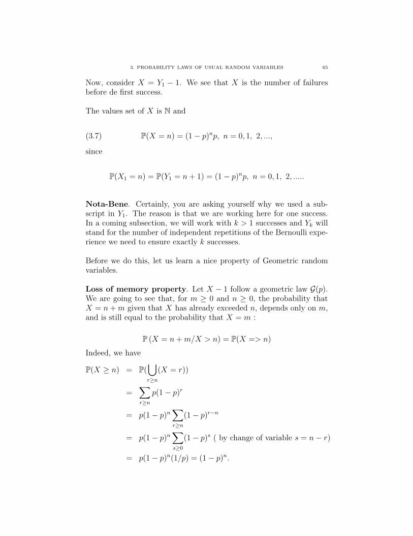
3. PROBABILITY LAWS OF USUAL RANDOM VARIABLES 65
Now, consider X = Y1 − 1. We see that X is the number of failuresbefore de first success.
The values set of X is N and
(3.7) P(X = n) = (1− p)np, n = 0, 1, 2, ...,
since
P(X1 = n) = P(Y1 = n+ 1) = (1− p)np, n = 0, 1, 2, .....
Nota-Bene. Certainly, you are asking yourself why we used a sub-script in Y1. The reason is that we are working here for one success.In a coming subsection, we will work with k > 1 successes and Yk willstand for the number of independent repetitions of the Bernoulli expe-rience we need to ensure exactly k successes.
Before we do this, let us learn a nice property of Geometric randomvariables.
Loss of memory property. Let X − 1 follow a geometric law G(p).We are going to see that, for m ≥ 0 and n ≥ 0, the probability thatX = n+m given that X has already exceeded n, depends only on m,and is still equal to the probability that X = m :
P (X = n+m/X > n) = P(X => n)
Indeed, we have
P(X ≥ n) = P(⋃r≥n
(X = r))
=∑r≥n
p(1− p)r
= p(1− p)n∑r≥n
(1− p)r−n
= p(1− p)n∑s≥0
(1− p)s ( by change of variable s = n− r)
= p(1− p)n(1/p) = (1− p)n.

66 4. RANDOM VARIABLES
Then for m ≥ 0 and n ≥ 0, the event (X = m + n) is included in(X > n), and then (X = m+ n,X > n) = (X = m+ n). By using thelatter equality, we have
P (X = n+m/X1 > n) =P(X = m+ n,X > n)
P(X > n)
=P(X = m+ n)
P(X > n)
=p(1− p)n+m
(1− p)n= p(1− p)m
= P(X = m)
We say that X has the property of forgetting the past or loosing thememory. This means the following : if we continuously repeat theBernoulli experience, then given any time n, the law of the number offailures before the first success after the time n, does not depend on nand still has the probability law (3.7).
(7) Negative Binomial Random variable: BN (k, p).
A Negative Binomial Random variable Yk with parameter k ≥ 1 andp ∈]0, 1[, denoted by X ∼ BN (k, p), takes its values in
V(X1) = k, k + 1, ...and
P(Yk = n) = pk(1− p)n, n = 0, 1, .......
Generation. Unlikely to the binomial case, we fix the number ofsuccesses. And we independently repeat a Bernoulli experience withprobability p ∈]0, 1[ until we reach k successes. The number X of ex-periences needed to reach k successes is called a Negative BinomialRandom variable or parameters p and k.
(1) For Binomial random variable X ∼ B(n, p), we set the number ofexperiences to n and search the probability that the number of successis equal to k : P(X = k).
(1) For a Negative Binomial random variable Yk ∼ NB(n, p), we setthe number of successes k and search the probability that the number

3. PROBABILITY LAWS OF USUAL RANDOM VARIABLES 67
of experiences needed to have k successes is equal to n : P(Yk = n).
Of course, we need at least k experiences to hope to get k successes.So, the values set of Yk is
V(X1) = k, k + 1, ....The event (Yk = n) occurs if and only if :
(1) The nth experience is successful.
(2) Among the (n−1) first experiences, we got exactly (k−1) successes.
By independence, the probability of the event (Yk = n) is the productof the probabilities of the described events in (1) and (2), denoteda× b. But a = p and b is the probability to get k− 1 successes in n− 1independent Bernoulli experiences with parameter p. Then, we have
b =
(n− 1k − 1
)pk−1 (1− p)(n−1)−(k−1).
By using, the product of probabilities a× b, we arrive at
P(Yk = n) =
(n− 1k − 1
)pk (1− p)n−k, n ≥ k.
(8) Poisson Random Variable P(λ).
A Poisson Random Variable with parameter λ > 0, denoted byP(λ) takes its values in N and
(3.8) P(X = k) =λk
k!e−λ, k = 0, 1, 2, ...
where λ is a positive number.
Here, we are not able to generate the Poisson law by a simpleexperience. Rather, we are going to show how to derive it by a limitprocedure from binomial random variables.
First, we have the show that Formula (3.8) satisfies (2.1). If this istrue, we say that Formula (3.8) is the probability law of some randomvariable taking its values in N.

68 4. RANDOM VARIABLES
Remind the the following expansion (from calculus courses)
(3.9) ex =+∞∑k=0
xk
k!, x ∈ R.
By using (3.9), we get
+∞∑k=0
P(X = k) =+∞∑k=0
λk
k!e−λ
= e−λ+∞∑k=0
λk
k!
= e−λe+λ = 1
A random variable whose probability law is given by (3.8) issaid to follow a Poisson law with parameter λ.
We are going to see how to derive it from a sequence binonial randomvariables.
Let Xn, a sequence of B(n, pn) random variables such that, as n→ +∞,
(3.10) pn → 0 and npn → λ, 0 < λ < +∞.
Theorem 3. Let
fn(k) =
(nk
)pk(1− p)n−k.
be the probability law of the random variable Xn and the probability lawof the Poisson random variable
f(k) =e−λλk
k!Suppose that (3.10) holds. Then, for any fixed k ∈ N, we have, asn→∞,
fn(k)→ f(k).
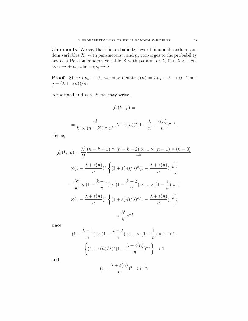
3. PROBABILITY LAWS OF USUAL RANDOM VARIABLES 69
Comments. We say that the probability laws of binomial random ran-dom variablesXn with parameters n and pn converges to the probabilitylaw of a Poisson random variable Z with parameter λ, 0 < λ < +∞,as n→ +∞, when npn → λ.
Proof. Since npn → λ, we may denote ε(n) = npn − λ → 0. Thenp = (λ+ ε(n))/n.
For k fixed and n > k, we may write,
fn(k, p) =
=n!
k!× (n− k)!× nk(λ+ ε(n))k(1− λ
n− ε(n)
n)n−k.
Hence,
fn(k, p) =λk
k!
(n− k + 1)× (n− k + 2)× ...× (n− 1)× (n− 0)
nk
×(1− λ+ ε(n)
n)n
(1 + ε(n)/λ)k(1− λ+ ε(n)
n)−k
=λk
k!× (1− k − 1
n)× (1− k − 2
n)× ...× (1− 1
n)× 1
×(1− λ+ ε(n)
n)n
(1 + ε(n)/λ)k(1− λ+ ε(n)
n)−k
→ λk
k!e−λ
since
(1− k − 1
n)× (1− k − 2
n)× ...× (1− 1
n)× 1→ 1,
(1 + ε(n)/λ)k(1− λ+ ε(n)
n)−k→ 1
and
(1− λ+ ε(n)
n)n → e−λ.

70 4. RANDOM VARIABLES
4. Independence of random variables
Definition 3. The discrete random variables X1, X2, . . ., Xn aremutually independent if and only if for any subset i1, i2, ..., ik of1, 2, ......, n and for any k-tuple (s1, ..., sk), we have the factorizingformula
P(Xi1 = s1, ..., Xik = sk) = P(Xi1 = s1)...P(Xik = sk)
The random variables X1, X2, . . . . . , Xn are pairwise independentif and only if for any 1 ≤ i 6= j ≤ n, for any si and sj, we have
P(Xi = si , Xj = sj) = P(Xi = si) P(Xj = sj).
Example 4. Consider a Bernoulli experience with parameter p ∈]0, 1[independently repeated. Set
Xi =
1 if the ith experience is successful
0 otherwise
Each Xi follows a Bernoulli law with parameter p, that is Xi ∼ B(p).
The random variables Xi are independent by construction. After n,repetitions, the number of successes X is exactly
X =n∑i=1
Xi.
We have the following conclusion : A Binomial random variable X ∼B(n, p) is always the sum of n independent random variables X1, ...,Xn, following all a Bernoulli law B(p).
Example 6. Consider a Bernoulli experience with parameter p ∈]0, 1[independently repeated.
Let T1 be the number of experiences needed to get one success.
Let T2 be the number of experiences needed to get one success afterthe first success.

4. INDEPENDENCE OF RANDOM VARIABLES 71
Generally, for i > 1, let Ti be the number of experiences needed to getone success after the (i− 1)th success.
It is clear that
T1 + ...+ Tkis the number of experiences needed to have k successes, that is
Yk = T1 + ...+ Tk
Because of the Memory loss property, the random variables Ti − 1 areindependent, so are the Ti. We get a conclusion that is similar to bi-nomial case.
Conclusion : a Negative Binomial random variable NB(k, p) is a sumof k independent random variables T1, ...,Tk following all a geometriclaw G(p).
Because of the importance of such results, we are going to statethem into lemmas.
Lemma 1. A Binomial random variable X ∼ B(n, p) is always thesum of n independent random variables X1, ..., Xn, following all aBernoulli law B(p).
and
Lemma 2. A Negative Binomial random variable NB(k, p) is a sumof k independent random variables T1, ...,Tk following all a geometriclaw G(p).


CHAPTER 5
Real-valued Random Variable Parameters
Before we begin, wee strongly stress that the mathematical expec-tation is defined only for a real-valued random variable. If a randomvariable is not a real-valued one, we may only have mathematical ex-pectation of real-valued functions of it.
1. Mean and Mathematical Expectation
Let us introduce the notion of mathematical expectation in an ev-ery day life example.
Example 1. Consider a class of 24 students. Suppose that 5 of themare 19 year old, 7 are 20 , 10 are 23, and 2 are 17. Let us denote by mthe mean age of the class, that is :
m =5× 19 + 7× 20 + 10× 23 + 2× 7
24= 20.79.
Let X be the random variable taking the distinct ages as values, thatis V(X) = x1, ..., x4 with x1 = 19, x2 = 20, x3 = 23, x4 = 17, withprobability law :
P(X = x1) =5
24, P(X = x2) =
7
24, P(X = x3) =
10
24, P(X = x4) =
3
24.
We may summarize this probability law in the following table :
k 19 20 23 17P (x = k) 5
24724
1024
324
Set Ω as the class of these 24 students. The following graph
X : Ω → Rω → X(ω)= age of the student ω.
defines a random variable. The probability that is used on Ω is thefrequency of occurrence. For each i ∈ 1, 2, 3, 4, P(X = xi) is the
73

74 5. REAL-VALUED RANDOM VARIABLE PARAMETERS
frequency of occurrence of the age xi in the class.
Through these notations, we have the following expression of the meanm :
(1.1) m =4∑i=1
xi P(X = xi).
The formula (1.1) is the expression of the mathematical expectation ofthe random variable X. Mean values in real life are particular casesof mathematical expectations in Probability Theory.
2. Definition and examples
Let X be a discrete real-valued random variable taking its valuesin V(X) = xi i ∈, I, where I is a subset of N. If the quantity
(2.1)∑i∈I
xi P(X = xi)
exists in R, we called it the mathematical expectation of X, denotedby E(X), and we write
E(X) =∑i∈I
xi P(X = xi).
If the quantity (2.1) is −∞ or +∞, we still name it the mathematicalexpectation, with E(X) = −∞ or E(X) = +∞.
We are now giving some examples.
Example 2. Let X be a degenerated random variable at c, that is
P(X = c) = 1
Then, Formula (2) reduces to :
E(X) = c× P(X = c) = c.
Let us keep in mind that the mathematical expectation of a constantis itself.
Example 3 Let X be Bernoulli random variable, X ∼ B(p), p ∈]0, 1[.Formula (2) is

3. GENERAL PROPERTIES OF THE MATHEMATICAL EXPECTATION 75
E(X) = 1× P(X = 1) + 0× P(X = 0) = p.
Exemple 4. Let X be a Binomial random variable, that is X ∼B(n, p), n ≥ 1 and p ∈]0, 1[. Formula (2) gives
E(X) =n∑k=0
k P(X = k) =n∑k=0
k n!
k!(n− k)!pk(1− p)n−k
=n∑k=1
np(n− 1)!
(k − 1)!(n− k)! pk−1(1− p)n−k
= npn∑k=1
Ck−1n−1 p
k−1(1− p)(n−1)−(k−1)
Let us make the change of variable : k′ = k− 1 and n′ = n− 1. By theNewton’s Formula in Theorem 1 in Chapter 1,
E(X) = npn′∑k′=0
(n′
k′
)pk′(1− p)n′−k′
= np (p+ (1− p))n′= np.
Exercise 1. Find the mathematical expectation of the a hypergeomet-ric H(N, r, θ) random variable, a Negative Binomial BN (k, p) randomvariable and a Poisson P(λ) random variable with N ≥ 1, 0 < r ≤ N ,θ ∈]0, 1[, n ≥ 1, p ∈]0, 1[, λ > 0.
Answers. We will find respectively : rθ ,(1− θ)(
1−rN
)and λ.
3. General Properties of the Mathematical Expectation
Let X and Y be two discrete random variables with respective set ofvalues xi, i ∈ Iand yj, j ∈ J. Let g anf h be two functions from Ronto R, k a function from R2 onto R. Finally, λ and µ are real numbers.
We suppose that all the mathematical expectations used below exist.We have the following properties.
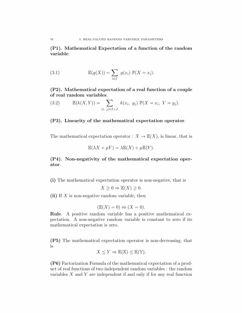
76 5. REAL-VALUED RANDOM VARIABLE PARAMETERS
(P1). Mathematical Expectation of a function of the randomvariable.
(3.1) E(g(X)) =∑i∈I
g(xi) P(X = xi).
(P2). Mathematical expectation of a real function of a coupleof real random variables.
(3.2) E(k(X, Y )) =∑
(i, j)∈I×J
k(xi, yj) P(X = xi, Y = yj).
(P3). Linearity of the mathematical expectation operator.
The mathematical expectation operator : X → E(X), is linear, that is
E(λX + µY ) = λE(X) + µE(Y ).
(P4). Non-negativity of the mathematical expectation oper-ator.
(i) The mathematical expectation operator is non-negative, that is
X ≥ 0⇒ E(X) ≥ 0.
(ii) If X is non-negative random variable, then
(E(X) = 0)⇔ (X = 0).
Rule. A positive random variable has a positive mathematical ex-pectation. A non-negative random variable is constant to zero if itsmathematical expectation is zero.
(P5) The mathematical expectation operator is non-decreasing, thatis
X ≤ Y ⇒ E(X) ≤ E(Y).
(P6) Factorization Formula of the mathematical expectation of a prod-uct of real functions of two independent random variables : the randomvariables X and Y are independent if and only if for any real function

3. GENERAL PROPERTIES OF THE MATHEMATICAL EXPECTATION 77
g of X and h of Y such that the mathematical expectations of X andof Y exist, we have
E(g(X)× h(Y )) = E(g(X))× E(h(Y ))
Remarks : In Formulas (P1), (P2) and (P6), the random variablesX and Y are not necessarily real-valued random variables. They maybe of any kind : vectors, categorical objects, etc.Proofs.
Proof of (P1). Set Z = g(X), X ∈ xi, i ∈ I. The values set of Zare the distinct values of g(xi), i ∈ I. Let us denote the values set byzk, k ∈ K, where necessarily, Card(K) ≤ Card(I), since
zk, k ∈ K ⊆ g(xi), i ∈ I .For each k ∈ K, we are going to define the class of all xi such thatg(xi) = zk, that is
Ik = i ∈ I , g(xi) = zk .It comes that for k ∈ K,
(Z = zk) = ∪i∈Ik
(X = xi).
It is also obvious that the Ik, k ∈ K, form a partition of I, that is
(3.3) I =∑k∈K
Ik.
Formula (3) implies that
(3.4) P(Z = zk) =∑i∈Ik
P(X = xi).
By definition, we have
(3.5) E(Z) =∑k∈K
zk P(Z = zk).
Let us combine all these facts to conclude. By the partition (3.3), wehave ∑
i∈I
g(xi) P(X = xi) =∑k∈K
∑i∈Ik
g(xi) P(X = xi).

78 5. REAL-VALUED RANDOM VARIABLE PARAMETERS
Now, we use the remark that g(xi) = zk on Ik, in the latter expression,to get
∑k∈K
∑i∈Ik
g(zk) P(X = xi) =∑k∈K
g(zk)
(∑i∈Ik
P(X = xi)
)=
∑k∈K
g(zk)P(Z = zk)
where we used (3.4) in the last line, which is (3.5). The proof is finished.
Proof of (P2). This proof of the property is very similar to that of(P1). Set V = k(X, Y ), X ∈ xi, i ∈ I and Y ∈ yj, j ∈ J. As inthe proof of (P1), V take the distinct values among the values k(xi, yj),(i, j) ∈ I × J , and we write
VV = vk, k ∈ K ⊆ k(xi, yj), (i, j) ∈ I × J .
Similarly, we partition VV in the following way :
Ik = (i, j) ∈ I × J, k(xi, yj) = vk .
so that
(3.6) I × J =∑k∈K
Ik.
and
(V = vk) = ∪(i,j)∈Ik
(X = xi, Y = yj).
Formula (3.4) implies
(3.7) P(V = vk) =∑
(i,j)∈Ik
P(X = xi, Y = yj).
By definition, we have
(3.8) E(V ) =∑k∈K
vk P(V = vk).
Next, by the partition (3.6), we have

3. GENERAL PROPERTIES OF THE MATHEMATICAL EXPECTATION 79
∑(i,j)∈I×J
k(xi, yj) P(X = xi, Y )yj)
=∑k∈K
∑i∈Ik
g(vk) P(X = xi)
Now, we use the remark that that k(xi, yj) = vk on Ik, in the latterexpression, to get
∑(i,j)∈I×J
k(xi, yj) P(X = xi, Y = yj)
=∑k∈K
∑i∈Ik
g(vk) P(X = xi, Y = yj)
=∑k∈K
g(vk)
(∑i∈Ik
P(X = xi, Y = yj)
)=
∑k∈K
g(vk)P(V = vk)
where we used (3.7) in the last line, which is (3.8). The proof is finished.
Proof of (P3). First, let us apply (P1) with g(X) = λX, to get
E(λX) =∑i∈I
λ xi P(X = xi) = λ E(X).
Next, we apply (P2) with k(x, y) = x+ y, to get
E(X + Y ) =∑
(i, j)∈I×J
(xi + yj) P(X = xi, Y = yj)
=∑i∈I
xi
∑j∈J
P(X = xi, Y = yj)
+∑j∈J
yj
∑i∈I
P(X = xi, Y = yj)
.
But
Ω = ∪j∈J
(Y = yj) =∑j∈J
(Y = yj).
Thus,
(X = xi) = (X = xi) ∩ Ω =∑j∈J
(X = xi, Y = yj),
and then

80 5. REAL-VALUED RANDOM VARIABLE PARAMETERS
P(X = xi) =∑j∈J
P(X = xi, Y = yj).
By the symmetry of the roles of X and Y , we also have
P(Y = yj) =∑i∈I
P(X = xi, Y = yj).
Finally,
E(X) =∑i∈I
xi P(X = xi) +∑j∈J
yj P(Y = yj) = E(X) + E(Y ).
We just finished the proof that the mathematical expectation is linear.lineaire.
Proof of (P4).
Part (i).
Let X ∈ xi, i ∈ I and X ≥ 0. This means that the values of X,which are the xi’s, are non-negative. Hence, we have
E(X) =∑i∈I
xi P(X = xi) ≥ 0,
as a sum of the product of xi and P(X = xi) both non-negative.
Part (ii).
Assume that X is non-negative. This means that the values xi arenon-negative. E(X) = 0 means that
E(X) =∑i∈I
xi P(X = xi) = 0.
Since the left-hand member of this equation is formed by a sum ofnon-negative terms, it is null if and only if each of the terms are null,that is for each i ∈ I,
xi P(X = xi) = 0.
Hence, if xi is a value if X, we have P(X = xi) > 0, and then xi. Thismeans that X only takes the value 0. Thus, we have X = 0.
Proof of (P5). Let X ≤ Y . By linearity and, since the mathematicalexpectation is a non-negative operator,

3. GENERAL PROPERTIES OF THE MATHEMATICAL EXPECTATION 81
0 ≤ E(Y −X) = E(Y )− E(X).
Hence E(Y ) ≥ E(X).
Proof of (P6). Suppose that X and Y are independent. Set k(x, y) =g(x)h(y). We may apply (P2) to get
E(g(X)h(Y )) =∑i, j
g(xi)h(yj) P(X = xi, Y = yj).
But, by independence,
P(X = xi, Y = yj) = P(X = xi) P(Y = yj),
for all (i, j) ∈ I × J . Then, we have
E(g(X)h(Y )) =∑j∈J
∑i∈I
g(xi) P(X = xi) h(yj) P(Y = yj)
=∑i∈I
g(xi) P(X = xi)×∑j∈J
h(yj) P(y = yj)
= E(g(X)) E(h(Y )).
This proves the direct implication.
Now, suppose that
E(g(X)h(Y )) = E(g(X))× E(h(Y )),
for all functions g and h for which the mathematical expectations makesenses. Consider two particular values in I × J , i0 ∈ I and j0 ∈ J . Set
g(x) =
0 si x 6= xi01 si x = xi0
and
h(y) =
0 if y 6= yj01 if y = yj0
We have

82 5. REAL-VALUED RANDOM VARIABLE PARAMETERS
E(g(X)h(Y )) =∑
(i, j)∈I×J
g(xi)h(yj) P(X = xi, Y = yj)
= P(X = xi0 , Y = yj0)
= Eg(X)× Eh(Y )
=∑i∈I
g(xi) P(X = xi) ×∑j∈J
h(yj)P(Y = yj)
= P(X = xi0) P(Y = yj0).
We proved that for any (i0, j0) ∈ I × J , we have
P(X = xi0 , Y = yj0) = P(X = xi0) P(Y = yi0)
We then have the independence.
4. Usual Parameters of Real-valued Random Variables
Let X and Y be a discrete real-valued random variables with re-spective values set xi, i ∈ I and yj, j ∈ J.
The most common parameters of such random variables are definedbelow.
4.1. Definitions. . We list below the names of some parametersand next give their expressions.
kth non centered moments or moments of order k ≥ 1 :
mk = E(Xk) =∑i∈I
xki P(X = xi)
Centered Moments of order k ≥ 1 :
Mk = E((X − E(X))k) =∑i∈I
(xi − E(X))k P(X = xi)
Variance and Standard deviation.
The variance of X is defined by :
σ2X = V ar(X) = E((X − E(X))2) =
∑i∈I
(xi − E(X))k P(X = xi)

4. USUAL PARAMETERS OF REAL-VALUED RANDOM VARIABLES 83
The square root of the variance of X, σX = (V ar(X))12 , is the standard
deviation of X.
Remark. The variance is the centered moment of order 2.
factorial moment of order two of X :
fm2(X) = E((X(X − 1)) =∑i∈I
xi (xi − 1) P(X = xi).
Covariance between X and Y :
Cov(X, Y ) = E((X−E(X))(E−E(Y ))) =∑i, j
(xi−E(X))(yi−E(Y )) P(X = xi, Y = yj).
Linear correlation coefficient between X and Y .
If σX 6= 0 and σY 6= 0, we may define the number
σXY =Cov(X, Y )
σX σYas the linear correlation coefficient.
Now, we are going to review important properties of these properties.
4.2. Properties.
(1) Other expression of the variance and the covariance.
(i) The variance and the covariance have the following two alternativeexpressions :
V ar(X) = E(X2)− E(X)2.
and
Cov(X, Y ) = E(XY )− E(X) E(Y ).
Rule. The variance is the difference of the non centered moment oforder two and the square of the mathematical expectation.
Rule. The covariance between X and Y is the difference of mathe-matical expectation of the product of X and Y and the product of the

84 5. REAL-VALUED RANDOM VARIABLE PARAMETERS
mathematical expectations of X and Y .
(ii) The variance can be computed form the factorial moment of order2 by
(4.1) V ar(X) = fm2(X) + E(X)2 − E(X)2.
Remark. In a number of cases, the computation of the second fac-torial moment is easier than that of the second moment, and Formula(4.1) becomes handy.
(2). The standard deviation or the variance is zero if andonly if the random variable is constant and is equal to itsmathematical expectation :
σX = 0 if and only if X = E(X)
(3) Variance of a linear combination of random variables.
(i) Variance of the sum of two random variables :
V ar(X + Y ) = V ar(X) + V ar(Y ) + 2Cov(X, Y ).
(ii) Independence and Covariance. If X and Y are independentthen
V ar(X + Y ) = V ar(X) + V ar(Y ) and Cov(X, Y ) = 0.
We conclude by :
(3ii-a) The variance of independent random variable is the sum of thevariance.
(3ii-b) If X and y are independent, they are uncorrelated that is,
Cov(X, Y ) = 0.
Two random variables X and y are linearly uncorrelated if and onlyCov(X, Y ). This is implied by the independence. But lack of correla-tion does not imply independence. This may happen for special class

4. USUAL PARAMETERS OF REAL-VALUED RANDOM VARIABLES 85
of random variables, like Gaussian ones.
(iii) Variance of linear combination of random variables.
Let Xi, i ≥ 1, be a sequence of real-valued random variables. Letai, i ≥ 1, be a sequence of real numbers. The variance of the linearcombination
k∑i=1
aiXi
is given by :
V ar(k∑i=1
aiXi) =k∑i=1
a2i V ar(Xi) + 2
∑1≤i<j≤k
aiaj Cov(Xi, Xj).
(4). Cauchy-Schwartzs inequality :
|Cov(X, Y )| ≤ σX σY .
(5). Holder Inequality.
Let p > 1 and q > 1 such that 1/p+ 1/q = 1. Suppose that
‖X‖p = E(|X|p)1/p
and
‖X‖q = E(|X|q)1/q
exists. Then
|E(XY )| ≤ ‖X‖p × ‖X‖p
(6) Minkowski’s Inequality.
For any p > 1,
‖X + Y ‖p ≤ ‖X‖p + ‖Y ‖p
The number ‖X‖p is called the Lp-norm of X.

86 5. REAL-VALUED RANDOM VARIABLE PARAMETERS
(7) Jensen’s Inequality.
if g : I 7→ R is a convex convex on an interval including VX , and if
E(|X|) =∑i∈I
pi|xi| < +∞
and
E(|g(X)|) =∑i∈I
pi|g(xi)| < +∞,
then
g(E(X)) ≤ E(g(X)).
Proofs. Let us provide the proofs of these properties one by one inthe same order in which they are stated.
Proof of (1).
Part (i). Let us apply the linearity of the mathematical expectationstated in Property (P3) above to the following development
(X − E(X))2 = X2 + 2XE(X) + E(X)2
to get :
V ar(X) = E(X − E(X))2 = E(X2 − 2 X E(X) + E(X)2)
= E(X2)− 2E(X)E(X) + E(X)2
= E(X2)− E(X)2.
We also have, by the same technique,
Cov(X, Y ) = E(X − E(X))(Y − E(Y ))
= E(XY −XE(Y )− Y E(X) + E(X) E(Y ))
= E(XY )− E(X) E(Y )(4.2)
Let us notice that the following identity
V ar(X) = Cov(X,X)
and next remark that the second formula implies the first.

4. USUAL PARAMETERS OF REAL-VALUED RANDOM VARIABLES 87
From the formula of the covariance, we see by applying Property (P6),that the independence of X and Y implies
E(XY ) = E(X)× E(Y )
and then
cov(X, Y ) = 0
Part (ii). It is enough to remark that
fm2(X) = E(X(X − 1)) = E(X2)− E(X),
and to use it the Formula of the variance above.
Proof of (2). Let us begin to prove the direct implication. AssumeσX = 0. Then
σ2X =
∑i
(xi − E(X))2 P(X = xi) = 0.
Since this sum of non-negative terms is null, each of the terms are null,that is for each i ∈ I,
(xi − E(X))2 P(X = xi) = 0.
Hence, if xi is a value if X, we have P(X = xi) > 0, and thenxi − E(X) = 0, that is xi = E(X). This means that X only takesthe value E(X).
Conversely, if X takes one unique value c, we have P(X = c) = 1.Then for any k ≥ 1,
E(Xk) = ck P(X = c) = ck.
Finally, the variance is
V ar(X) = E(X2)− E(X)2 = c2 − c2 = 0.
Proof of (3). We begin by the general case of a linear combination of
random variables of the form Y =∑k
i=1 aiXi. By the linearity Property(P6) of the mathematical expectation, we have
E(Y) =k∑i=1
aiE(Xi).

88 5. REAL-VALUED RANDOM VARIABLE PARAMETERS
It comes
Y − E(Y) =k∑i=1
ai(Xi − E(Xi)).
Now, we use the full development of products of two sums
(Y−E(Y ))2 =k∑i=1
a2i (Xi−E(Xi))
2+2∑
1≤i<j≤k
aiaj (Xi−E(Xi))(Xj−E(Xj)).
We apply the mathematical expectation of the this formula to get
V ar(Y ) =k∑i=1
a2i V ar(Xi) + 2
∑1≤i<j≤k
aiaj Cov(Xi, Xj).
In particular If X1,...,Xk are pairwise independent (let alone mutuallyindependent), then
V ar(Y ) =k∑i=1
a2iV ar(Xi)
Proof of (4). We are going to proof the Cauchy-Schwartzs inequalityby studying the sign of the trinomial function V arX + λ2V ar(Y ) +2λCov(X, Y ), where λ ∈ R.
We begin to remark that if V ar(Y ) = 0, then by Point (2) above, Y isa constant, say c = E(Y ). Since Y − E(Y ) = c− c, this implies that
cov(X, c) = E(X − E(X))(Y − E(Y ))) = E(X − E(X))(0) = 0.
In that case, the inequality
|cov(X, Y )| ≤ σXσX ,
is true, since the two members are both zero.
Now suppose that V ar(Y ) > 0. By using Point (3) above, we have
V ar(X + λ Y ) = V arX + λ2V ar(Y ) + 2λCov(X, Y ).
Then we get that the trinomial function V arX+λ2V ar(Y )+2λCov(X, Y )in λ has the constant non-negative sign. This is possible if and only ifthe discriminant is non-positive, that is
∆′ = Cov(X, Y )2 − V arX × V arY ≤ 0.

4. USUAL PARAMETERS OF REAL-VALUED RANDOM VARIABLES 89
This leads to
Cov(X, Y )2 ≤ V arX × V arY.By taking the square roots, we get
|cov(X, Y )| ≤ σXσX ,
which is the searched result.
Proof of (5). We are going to use the following inequality if R :
(4.3) |ab| ≤ |a|p
p+|b|q
q.
We may easily check if p and q are positive integers such that 1/p +1/q = 1, the both of p and q are greater that the unity and the formulas
p =q
q − 1and q =
p
p− 1.
also hold. Assume first that we have : ‖X‖p 6= 0 and ‖Y ‖q 6= 0. Set
a =X
‖X‖pand b =
Y
‖Y ‖q.
By using Inequality (4.3), we have
|X × Y |‖X‖p × ‖Y ‖q
≤ |X|p
p× ‖X‖pp+
|Y |q
q × ‖Y ‖qq.
By taking the mathematical expectation, we obtain
E |X × Y |‖X‖p × ‖Y ‖q
≤ E |X|p
p× ‖X‖pp+
E |Y |q
q × ‖Y ‖qq.
This yields
E |X × Y |‖X‖p × ‖Y ‖q
≤ 1
p+
1
q= 1.
We proved the inequality if neither of ‖X‖p and ‖Y ‖q are null. If one
of them is zero, say ‖X‖p, this mean that
E(|X|p) = 0.

90 5. REAL-VALUED RANDOM VARIABLE PARAMETERS
By Property Point (ii) of Property (p4) above, |X|p = 0 and henceX = 0.
In this case, both members in the Holder inequality are zero and then,it holds.
Proof of (6). We are going to use the Holder inequality to establishthe Minkowski’s one.
First, if ‖X + Y ‖p = 0, there is nothing to prove. Now, suppose that
‖X + Y ‖p > 0.
We have
|X + Y |p = |X + Y |p−1 |X + Y | ≤ |X + Y |p−1 |X|+ |X + Y |p−1 |Y |By taking the expectations, and by using the Holder to each of the twoterms the right-hand member of the inequality and by reminding thatq = (p− 1)/p, we get
E |X + Y |p ≤ E |X + Y |p−1 |X|+ E |X + Y |p−1 |Y |≤ (E |X|p)1/p × E (|X + Y |q(p−1))1/q + (E |Y |p)1/p × (E |X + Y |q(p−1))1/q.
Now, we divide the last formula by
(E |X + Y |q(p−1))1/q = (E |X + Y |p)1/q,
which is not null, to get
(E |X + Y |p)1−1/q ≤ ‖X‖p + ‖Y ‖p .
This was the target.
Proof of (7). Let g : I → R be a convex function such that I includesVX . We will see two particular cases and a general case.
Case 1 : VX is finite. In that case, let us denote VX = x1, · · · , xk,k ≥ 1. If g is convex, then by Formula (2.2) in Section 2 in theAppendix Chapter 8, Part (D-D1), we have
(4.4) g(p1x1 + ...+ pkxk) ≤ pkg(x1) + ...+ pkg(xk)
By the property (P1) of the mathematical expectation above, the left-hand member of this inequality is g(E(X)) and the right-hand member

4. USUAL PARAMETERS OF REAL-VALUED RANDOM VARIABLES 91
is E(g(X)).
Case 2 : VX is countable infinite, g is a bounded function or I is abounded and closed interval. In that case, let us denote VX = xi, i ≥1. If g is convex, then by Formula (2.3) Section 2 in the AppendixChapter 8 , Part (D-D2), we have
(4.5) g(p1x1 + ...+ pkxk) ≤ pkg(x1) + ...+ pkg(xk)
By the property (P1) of the mathematical expectation above, the left-hand member of this inequality is g(E(X)) and the right-hand memberis E(g(X)).
Case 3 : Let us suppose that VX is countable infinite only. DenoteVX = xi, i ≥ 1. Here, g is defined on the whole real line R. LetJn = [−n, n], n ≥ 1. Put, for n ≥ 1,
In = i, xi ∈ Jn,
Vn = xi, i ∈ Inand
p(n) =∑i∈In
pi.
Let Xn be a random variable taking the values of Vn = xi, i ∈ Inwith the probabilities
pi,n = pi/p(n).
By applying the Case 1, we have g(E(Xn)) ≤ Eg(Xn), which is
(4.6) g(∑i∈In
pi,nxi) ≤∑i∈In
pi,ng(xi).
Here we apply the dominated convergence theory of the Section 3 inthe Appendix Section 8. We have∣∣∣∣∣∑
i≥1
pixi1(xi∈Jn)
∣∣∣∣∣ ≤∑i≥1
pi|xi| < +∞
and each pixi1(xi∈Jn) converges to pixi as n → +∞. Then, by thedominated convergence theorem for series, we have
(4.7)∑i≥1
pixi1(xi∈Jn) →∑i≥0
pixi.

92 5. REAL-VALUED RANDOM VARIABLE PARAMETERS
The same argument based on the finiteness of∑
i≥0 pi|xi| impliesthat
(4.8)∑i≥1
pig(xi)1(xi∈Jn) →∑i≥0
pig(xi).
We referring to Section 2 in the Appendix Chapter 8, Part B, we knowthat a convex function g is continuous. We may also remark that p(n)converges to the unity as n→ +∞. By combinig these facts with 4.2,we have
(4.9)∑i≥1
pixi1(xi∈Jn) + (1− p(n)pixi1(xi∈Jn →∑i≥0
pixi.
and
g(∑i≥1
pixi) = limn→+∞
g(∑i≥1
pixi1(xi∈Jn + (1− p(n))∑i≥1
pixi1(xi∈Jn)
which is
g(∑i≥1
pixi) = limn→+∞
g(p(n)∑i≥1
pi,nxi1(xi∈Jn + (1− p(n))∑i≥1
pixi1(xi∈Jn)
By convexity of g, we have
g(∑i≥1
pixi) = limn→+∞
p(n)g
(∑i≥1
pi,nxi1(xi∈Jn)
)+(1−p(n))g
(∑i≥1
pixi1(xi∈Jn)
)We may write it as
g(∑i≥1
pixi) = limn→+∞
p(n)g
(∑i∈In
pi,nxi
)+ (1− p(n))g
(∑i∈In
pixi
)By using Formula in the first term of the left-hand member of the latterinequality, we have
g(∑i≥1
pixi) = limn→+∞
p(n)∑i∈In
pi,ng(xi) + (1− p(n))g
(∑i∈In
pixi1(xi∈Jn)
).
This gives

4. USUAL PARAMETERS OF REAL-VALUED RANDOM VARIABLES 93
g(∑i≥1
pixi) = limn→+∞
∑i∈In
pig(xi) + (1− p(n))g
(∑i∈In
pixi1(xi∈Jn)
).
Finally, we have
g(∑i≥1
pixi) ≤∑i≥0
pig(xi) + 0× g
(∑i≥0
pixi
).
which is exactly
g(E(X)) ≤ E(g(X)).

94 5. REAL-VALUED RANDOM VARIABLE PARAMETERS
5. Parameters of Usual Probability law
We are going to find the most common parameters of usual real-valuedrandom variables. It is recommended to know these results by heart.
In each example, we will apply Formula (3.1) and (3.2) to perform thecomputations.
(a) Bernoulli Random variable : X ∼ B(p).
We have
E(X) = 1 P(X = 1) + 0 P(X = 0) = p
E(X2) = 12P(X = 1) + 0P(X = 0) = p2.
We conclude :
V ar(X) = p(1− p) = pq.
(b) Binomial Random variable Yn ∼ B(n, p).
We have, by Lemma 1 of Chapter 4,
Yn =n∑i=1
Xi
where X1, ..., Xn are Bernoulli B(p) random variables. We are goingto use the known parameters of the Bernoulli random variables. Bylinearity property (P3), its comes that
E(Yn) =n∑i=1
E(Xi) = np
and by variance-covariance properties in Point (3) above, the inde-pendence of the Xi’s allows to conclude that
V ar(Yn) =n∑i=1
V ar(Xi) = npq.
(c) Geometric Random Variable : X ∼ G(p), p ∈]0, 1[.
Remind that

5. PARAMETERS OF USUAL PROBABILITY LAW 95
P(X = k) = p(1− p)k−1, k = 1, 2....
Hence
E(X) =∞∑k=1
k p(1− p)k−1
= p
(∞∑k=1
kqk−1
)
= p
(∞∑k=0
qk
)′(use the primitive here)
= p
(1
1− q
)′=
p
(1− q)2
=p
p2=
1
p.
Its factorial moment of second order is
E(X(X − 1)) = p∞∑k=1
k(k − 1)qk−1 = pq∞∑k=2
k(k − 1)qk−2
= pq
(∞∑k=0
qk
)′′(Use the primitive twice )
= pq
(1
(1− q)2
)′= 2pq(1− q)−3 =
2pq
p3=
2q
p2.
Thus, we get
E(X2) = E(X(X − 1)) + E(X) =2q
p2+
1
p,
and finally arrive at
(5.1) V ar(X) =2q
p2+
1
p− 1
p2=
q
p2.
In summary :
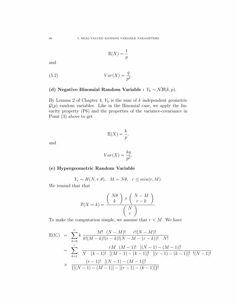
96 5. REAL-VALUED RANDOM VARIABLE PARAMETERS
E(X) =1
pand
(5.2) V ar(X) =q
p2.
(d) Negative Binomial Random Variable : Yk ∼ NB(k, p).
By Lemma 2 of Chapter 4, Yk is the sum of k independent geometricG(p) random variables. Like in the Binomial case, we apply the lin-earity property (P6) and the properties of the variance-covariance inPoint (3) above to get
E(X) =k
p.
and
V ar(X) =kq
p2.
(e) Hypergeometric Random Variable
Yr ∼ H(N, r, θ), M = Nθ, r ≤ min(r,M).
We remind that that
P(X = k) =
(Nθk
)×(N −Mr − k
)(Nr
) .
To make the computation simple, we assume that r < M . We have
E(Yr) =r∑
k=0
kM ! (N −M)! r!(N −M)!
k!(M − k)!(r − k)!(N −M − (r − k))! N !
=r∑
k=1
rM (M − 1)! [(N − 1)− (M − 1)]!
N (k − 1)! [(M − 1)− (k − 1)]! [(r − 1)− (k − 1)]! !(N − 1)!
× (r − 1)! [(N − 1)− (M − 1)]!
[(N − 1)− (M − 1)]− [(r − 1)− (k − 1)]!

5. PARAMETERS OF USUAL PROBABILITY LAW 97
Let us make the following changes of variables k′ = k−1, M ′ = M −1,r′ = r − 1, N ′ = N − 1. We get
E(Yr) =rM
N
[r′∑
k′=0
Ck′
M ′Cr′−k′N ′−M ′
Cr′N ′
]=rM
N= rθ,
since, the term in the bracket is the sum of probabilities of a Hyperge-ormetric random variableH(N−1, r−1, θ′), with θ′ = (M−1)/(N−1),then it is equal to one.
The factorial moment of second order is
E(Yn(Yn − 1)) =n∑k=2
k(k − 1)M ! (N −M)! n!(N − n)!
k! (M − k)! (N −M − (n− k))! (n− k)! N !.
Then we wake the changes of variables k′′ = k − 2, M ′′ = M − 2,N ′′ = N − 2, r′′ = r − 2, to get
E(Yr(Yr − 1)) =Mr(M − 1)(r − 1)
N(N − 1)
[r′′∑
k′′=0
Ck′′
M ′′Cr′′−k′′N ′′−M ′′
Cr′′N ′′
].
since, the term in the bracket is the sum of probabilities of a Hypergeor-metric random variable H(N−2, r−2, θ′′), with θ′′ = (M−2)/(N−2),and then is equal to one.
We get
E(Yr(Yr − 1) =M(M − 1) r(r − 1)
N(N − 1),
and finally,
V arYr =M(M − 1) r(r − 1)
N(N − 1)+rM
N− r2M2
N2
= rM
N(N −MN
)(1− rN
).
In summary, we have
E(Yr) = rθ
and

98 5. REAL-VALUED RANDOM VARIABLE PARAMETERS
V ar Yr = rθ(1− θ)(1− f),
where
f =r
N
(f) Poisson Random Variable : X ∼ P(λ), λ > 0.
We remind that
P(X = k) =λk
k!e−λ
for k = 0, 1, .... Then
E(X) =∞∑k=0
k × λk
k!e−λ
=∞∑k=1
λk
(k − 1)!e−λ
= λ∞∑k=1
λk−1
(k − 1)!e−λ
By setting k′ = k − 1, we have
E(X) = λe−λ∞∑k′=0
λk′
k′!
= λe−λeλ
= λ.
The factorial moment of second order is
E(X(X − 1)) =∞∑k=0
k(k − 1)× λk
k!e−λ
=∞∑k=2
λk
(k − 2)!e−λ
= λ2e−λ∞∑k=1
λk−2
(k − 2)!

5. PARAMETERS OF USUAL PROBABILITY LAW 99
By putting k′′ = k − 1, we get
E(X(X − 1)) = λ2e−λ∞∑
k′′=0
λk′
k′!
= λ2.
HenceE(X2) = E(X(X − 1)) + E(X) = λ2 + λ
and then we haveV ar(X) = λ
Remark. For a Poisson random variable, the mathematical expecta-tion and the variance are both equal to the intensity λ.

100 5. REAL-VALUED RANDOM VARIABLE PARAMETERS
6. Importance of the mean and the standard deviation
Let us denote the mean of a random variable X by m. The meanis meant to be a central parameter of X and it is expected that thevalues of X are near the mean m. This is not always true. Actually,the standard deviation measures how the values are near the mean.
We already saw in Property (P3) that a null standard deviation meansthat there is no deviation from the mean and that X is exactly equalto the mean.
Now, in a general case, the Tchebychev inequality may be used tomeasure the deviation of a random variable X from its mean. Here isthat inequality :
Proposition 1. (Tchebychev Inequality). if σ2X = V ar(X) >
0, then for any λ > 0, we have
P(|X − E(X)| > λ σX) ≤ 1
λ2.
Commentary. This inequality says that the probability that X devi-ates from its mean by at least λσX is less than one over λ.
In general terms, we say this : that X deviates from its mean by atleast a multiple of σX is all the more unlikely that multiple is large.More precisely, the probability that that X deviates from its mean byat least a multiple of σX is bounded by the inverse of the square of thatmultiple. This conveys the fact that the standard deviation controlshow the observations are near the mean.
Proof. Let us begin to prove the Markov’s inequality. Let Y be anon-negative random variable with values yj, j ∈ J. Then, for anyλ > 0, the following Markov Inequality
(6.1) P(Y > E(Y )) <1
λ,
holds. Before we give the proof of this inequality, we make a remark.By the formula in Theorem 2 on Chapter 4, we have for any number y,
(6.2) P(Y ≤ y) =∼ yi ≤ yP(Y = yi).

6. IMPORTANCE OF THE MEAN AND THE STANDARD DEVIATION 101
Let us give now the proof of the inequality (6.1). Since, by the assump-tions, yj ≥ 0 for all j ∈ J , we have
E(Y ) =∑j∈J
yjP(Y = yj)
=∑
yj≤λE(Y )
yjP(Y = yi) +∑
yj>λE(Y )
yjP(Y = yj).
Then by getting rid of the first term and use Formula (6.2) to get
E(Y ) ≥∑
yj>λE(Y )
yjP(Y = yj)
≥ (λE(Y ))×∑
yj>λE(Y )
P(Y = yj)
= (λE(Y ))× P(Y > λE(Y )).
By comparing the two extreme members of this latter formula, we getthe Markov inequality in Formula (6.1).
Now, let us apply the Markov’s inequality to the random variable
Y = (X − E(X))2.
By definition, we have E(Y ) = V ar(X) = σ2. The application ofMarkov’s inequality to Y leads to
P(|X − E(X)| > λσ) = P(|X − E(X)|2 > λ2σ2)
≤ 1
λ2.
An this finishes the proof.
Application of the Tchebychev’s Inequality : Confidence in-tervals of X around the mean.
The Chebychev’s inequality allows to describe the deviation of the ran-dom variable X from mean mX in the following probability covering
(6.3) P (mX −∆ ≤ X ≤ m+ ∆) ≥ 1− α.This relation say that we are 100(1 − α)% confident that X lies inthe interval I(m) = [m − ∆m,m + ∆m]. If Formula (6.3) holds,
102 5. REAL-VALUED RANDOM VARIABLE PARAMETERS
I(mX) = [mX−∆,mX +∆] is called a (1−α)-confidence interval of X.
By using the Chebychev’s inequality, I(mX , α) = [mX−σX/√α,mX +
σX/√α] is a (1− α)-confidence interval of X, that is
(6.4) P(mX −
σX√α≤ X ≤ mX +
σX√α
)≥ 1− α.
Let us make two remarks.
(1) The confidence intervals are generally used for small values of α,and most commonly for α = 5%. And we have a 95% confidence intervalof X in the form (since 1/
√α = 4.47)
(6.5) P (mX − 4.47 σX ≤ X ≤ mX + 4.47σX) ≥ 95%.
95%-confidence intervals are used for comparing different groups withrespect to the same character X.
(2) Denote by
RV CX =∣∣∣ σm
∣∣∣ .Formula 6.4 gives for 0 < α < 1,
P(
1 +RV CX√
α≤∣∣∣∣Xm∣∣∣∣ ≤ 1 +
RV CX√α
)≥ α.
The coefficient RV CX is called the Relative Variation Coefficient of Xwhich indicates how small the variable X deviates from its mean. Gen-erally, it is expected that RV CX is less 30% for a homogeneous variable.
(3) The confidence intervals obtained by the Tchebychev’s inequalityare not not so precise as we may need them. Actually, they are mainlyused for theoretical purposes. In Applied Statistics analysis, more so-phisticated confidence intervals are used. For example, normal confi-dence interval are systematically exploited. But for learning purposes,Tchebychev confidence intervals are good tools.
Let us now prove Formula (6.4).

6. IMPORTANCE OF THE MEAN AND THE STANDARD DEVIATION 103
Proof of Formula 6.4. Fix 0 < α < 1 and ε > 0. Let us apply theChebychev inequality to get
P(|X − E(X)| > ε) = P(|X − E(X)| > ((ε
σX) σ)) ≤ σ2
X
ε2.
Let
α =σ2X
ε2.
We get
ε =σX√α
and then
P(|X −mX | >
σX√α
)≤ α,
which equivalent to
P(|X −mX | ≤
σX√α
)≥ 1− α,
and this is Formula (6.3).


CHAPTER 6
Random couples
This chapter is devoted to an introduction to the study of probabil-ity laws and usual parameters of random couples (X,Y) and relatedconcepts. Its follows the lines of Chapters 4 and 5 which focused onreal-valued random variables. As in the aforementioned chapter, hereagain, we focus on discrete random couples.
1. Strict and Extended Values Set for a Discrete RandomVariable
A discrete random couple (X, Y ) takes its values in a set of the form
SV(X,Y ) = (ai, bj), (i, j) ∈ K,where K is an enumerable set with
(1.1) ∀(i, j) ∈ K, P((X, Y ) = (ai, bj)) > 0.
We say that SV(X,Y ) is a strict support or a domain or a values set ofthe random couple (X, Y ), if and only if, all its elements are taken by(X, Y ) with a nonzero probabilities, as in (1.1). Remark for once thatadding to SV(X,Y ) supplementary points (x, y) which are not taken by(X, Y ), meaning that P((X, Y ) = (x, y)) = 0, does not change anythingregarding computations using the probability law of (X, Y ). If we havesuch points in a values set, we call this latter an extended values set.
We consider the first projections of the couple values defined as follows:
(ai, bj) → ai.
By forming a set of these projections, we obtain a set
VX = xh, h ∈ I.For any i ∈ I, xi is equal to one of the projections ai for which thereexists at least one bj such that (ai, bj) ∈ SV(X,Y ). It is clear that VX is
105

106 6. RANDOM COUPLES
the strict values set of X.
We have to pay attention to the possibility of having some values xithat are repeated while taking all the projections (ai, bj) → ai. Let usgive an example.
Let
(1.2) SV(X,Y ) = (1, 2), (1, 3), (2, 2), (2, 4)
with P((X, Y ) = (1, 2)) = 0.2,P((X, Y ) = (1, 3)) = 0.3,P((X, Y ) =(2, 2)) = 0.1 and P((X, Y ) = (2, 4)) = 0.4..
We have
VX = 1, 2.Here the projections (ai, bj) → ai give the value 1 two times and thevalue 2 two times.
We may and do proceed similarly for the second projections
(ai, bj) → bi,
to define
VY = yj, j ∈ J,as the strict values set of Y .
We express a strong warning to not think that the strict values set ofthe couple is the Cartesian product of the two strict values sets of Xand Y , that is
SV(X,Y ) = VX × VY .In the example of (1.2), we may check that
VX × VY = 1, 2 × 2, 3, 4= (1, 2), (1, 3), (1, 4), (2, 2), (2, 3), (2, 4)6= (1, 2), (1, 3), (2, 2), (2, 4)= SV(X,Y ).
Now, even we have this fact, we may use
V(X,Y ) = VX × VY ,

2. JOINT PROBABILITY LAW AND MARGINAL PROBABILITY LAWS 107
as an extended values set and remind ourselves that some of the ele-ments of V(X,Y ) may be assigned null probabilities by P(X,Y ).
In our example (1.2), using the extended values sets leads to the prob-ability law represented in Table 1.
Table 1. Simple example of a probability law in dimension 2
X \ Y 2 3 4 X1 0.2 0.3 0 0.52 0 0.1 0.4 0.5Y 0.2 0.4 0.4 1
In this table,
(1) We put the probability P((X, Y ) = (x, y)) at the intersection of thevalue x of X (in line) and the value y of Y (in column).
(2) In the column X, we put, at each line corresponding to a value x ofX, the sum of all the probability of that line. This column representsthe probability law of X, as we will see it soon.
(3) In the line Y , we put, at each column corresponding to a value y ofY , the sum of all the probability of that column. This line representsthe probability law of Y .
Conclusion. In our study of random couples (X, Y ), we always mayuse an extended values set of the form
V(X,Y ) = VX × VY ,
where VX is the strict values set of X and VY the strict values set ofY . If VX and VY are finite with relatively small sizes, we may appealto tables like Table 1 to represent the probability law of (X, Y ).
2. Joint Probability Law and Marginal Probability Laws
.Let (X, Y ) be a discrete random couple such that VX = xi, i ∈ I isthe strict values set of X and VY = yj, j ∈ J the strict values set ofY , with I ⊂ N and J ⊂ N. The probability law of (X, Y ) is given onthe extended values set

108 6. RANDOM COUPLES
V(X,Y ) = VX × VY ,by
(2.1) P(X = xi, Y = yj), (i, j) ∈ I × J.
where the event (X = xi, Y = yj) is a notation of the intersection(X = xi) ∩ (Y = yj).
This probability law may be summarized in Table 2.
X Y y1 ................ yj ................ Xx1 P(X = x1, Y = y1) ................ P(X = x1, Y = yj) ................ P(X = x1)x2 P(X = x2, Y = y1) ................ P(X = x2, Y = yj) ................ P(X = x2).... ................................. ................ ................................. ................ ...................xi P(X = xi, Y = y1) ............... P(X = xi, Y = yj) ................ P(X = xi)... ................................. ................ ................................. ................ ...................Y P(Y = y1) .............. P(Y = yj) ............... 100%
This table is formed as follows :
(1) We put the probability P((X, Y ) = (xi, yj)) at the intersection ofthe value xi of X (in line) and the value yj of Y (in column).
(2) In the column X, we put, at each line the corresponding to a valuexi of X, the sum of all the probability of that line. As we will see itlater, this column represents the probability law of X.
(3) In the line Y , we put, at each column corresponding to a value y ofY , the sum of all the probability of that column. This line representsthe probability law of Y .
Let us introduce the following terminology.
Joint Probability Law.
The joint probability law of (X, Y ) is simply the probability law of thecouple, which is given in (2.1).

2. JOINT PROBABILITY LAW AND MARGINAL PROBABILITY LAWS 109
Marginal probability laws.
The probability laws of X and Y are called marginal probability laws.
Here is how we get the marginal probability law of X and Y from thejoint probability law. Let us begin by X.
We already knew, from Formula (2.3), that any event B can be decom-posed into
B =∑j ∈ J
B ∩ (Y = yj).
So, for a fixed i ∈ I, we have
(X = xi) =∑j ∈ J
(X = xi) ∩ (Y = yj) =∑j ∈ J
(X = xi, Y = yj).
By applying the additivity of the probability measure, it comes that
(2.2) P(X = xi) =∑j ∈ J
P(X = xi, Y = yj), i ∈ I.
By doing the same of Y , we get
(2.3) P(Y = yj) =∑i ∈ I
P(X = xi, Y = yj), j ∈ J.
We may conclude as follows.
(1) The marginal probability law of X, given is (2.2) is obtained bysumming the joint probability law over the values of Y .
In Table 2, the marginal probability law of X is represented by the lastcolumn, in which each line corresponding to a value xi of X is the sumof all the probability of that line.
(2) The marginal probability law of Y , given is (2.3) is obtained bysumming the joint probability law over the values of X.
In Table 2, the marginal probability law of Y is represented by the lastline, in which each column corresponding to a value yj of Y is the sumof all the probability of that column.

110 6. RANDOM COUPLES
(3) The box at the intersection of the last line and the last column con-tains the unit value, that is, at the same time, the sum of all the jointprobabilities, all marginal probabilities of X and all marginal proba-bilities of Y .
Usually, it is convenient to use the following notations :
(2.4) pi,j = P(X = xi, Y = yj), (i, j) ∈ I × J.
(2.5) pi,. = P(X = xi), i ∈ I.and
(2.6) p.,j = P(Y = yj), j ∈ J.
We have the formulas
pi,. = P(X = xi, Y ∈ Ω)(2.7)
=∑j ∈ J
pi,j i ∈ I.(2.8)
and
p.,j = P(X ∈ Ω, Y = yj)(2.9)
=∑i ∈ I
pi,j, j ∈ J.(2.10)
3. Independence
We come back to the concept of conditional probability and in-dependence that was introduced in Chapter 3. This section is devel-oped for real-values random variables. But we should keep in mindthat the theory is still valid for E-valued random variables, whereE = Rk. When a result hold only for real-valued random variables,we will clearly specify it.
I - Independence.

3. INDEPENDENCE 111
(a) Definition.
We remind that, by definition (see Property (P6) in Chapter 5), X andY are independent if and only if one of the following assertions holds.
(CI1) For all i ∈ J and j ∈ J ,
pij = pi,. × p.,j.(CI2) For any subsets A and B of E = R
P(X ∈ A, Y ∈ B) = P(X ∈ A)× P(Y ∈ B)
(CI3) For any non negative functions f, g : Ω 7→ E,
E(h(X)g(Y )) = E(h(X))× E(g(X))
Actually, Property (P6) in Chapter 5, only establishes the equivalencebetween (CI1) and (CI3). But clearly, (CI3) implies (CI2) by using thefollowing functions
h = 1A and g = 1A.
Also (CI2) implies (CI1) by using
A = xi and B = yj.
We get the equivalence between the three assertions by the circularargument :
(CI1)⇒ (CI3)⇒ (CI2)⇒ (CI1).
(b) New tools for assessing the independence.
For a real-valued random variable X, we may define the two fol-lowing functions depending on the law of X.
(MGF1) The first moment generating function of X :
ΦX(s) = E(exp(sX)) =∑i∈I
P(X = xi) exp(sxi), s ∈ R.
(MGF2) The second moment generating function of X :

112 6. RANDOM COUPLES
ΨX(s) = E(sX) =∑i∈I
P(X = xi)sxi , s ∈]0, 1].
It is clear that we have the following relation between these two func-tions :
(3.1) ΨX(s) = ΦX(log s) andΨX(1) = ΦX(0).
So, we do not need to study them separately. It is enough to study oneof them and to transfer the obtained properties to the other. Since,the first is more popular, we will study it. Consequently, the first formis simply called the moment generating function (m.g.f). When we usethe form given in (MGF2), we will call it by its full name as the secondm.g.t.
Characterization of probability laws. We admit that the m.g.tof X, when it is defined, is characteristic of the probability law of X,meaning that two real-valued random variables having the same m.g.thave the same law. The same characterization is valid for the secondm.g.t, because of the relation between the two m.g.f forms throughFormula (3.1). The proof of this result, which is beyond the level ofthis book, will be presented in the monograph [Lo (2016)] of this se-ries.
Each form of m.g.f has its own merits and properties. We have to usethem in smart ways depending of the context.
The m.g.f for real-valued random variables may be extended to a coupleof random variables. If X and Y are both real applications, we maydefine the bi-dimensional m.g.t of the couple (X, Y ) by
(MGFC)
ΦX,Y (s, t) = E(exp(sX+Y t)) =∑
(i,j)∈I×J
P(X = xi, Y = yi) exp(sxi+tyj),
for (s, t) ∈ R2.
The m.g.t has a nice and simple affine transformation formula. Indeed,if a and b are real numbers, we have for any for any s ∈ R
exp((aX + bs)) = ebs exp((as)X)

3. INDEPENDENCE 113
and then, we have
ΦZ(s) = E(exp((aX + b)s)
= E(ebs exp((as)X)
= ebsE(exp((as)X)
= ebsΦX(as).
We obtained this remarkable formula : for any real numbers a and b,for any s ∈ R, we have
(3.2) ΦaX+b(s) = ebsΦX(as)..
Formula (3.2) is a useful too, to find news probability laws for known
ones.
We are going to see two other interesting properties of these functions.
A - Moment generating Functions and Independence.
If X and Y are real-valued independent random variables, then we have:
For any s ∈ R,
(3.3) ΦX+Y (s) = ΨX(s)× ΦY (s), .
For any (s, t) ∈ R2,
(3.4) Φ(X,Y )(s, t) = ΨX(s)× ΦY (t).
Before we give the proofs, let us enrich our list of independent condi-tions.
(CI4) Two real-valued random variables X and Y are inde-pendent if and only Formula (3.4) holds for any (s, t) ∈ R2.

114 6. RANDOM COUPLES
This assertion also is beyond the current level. We admit it. We willprove it in [Lo (2016)].
Warning. Formula (3.4) characterizes the independence between tworandom variables, but not (3.3). Let us show it with this counter-example in [Stayonov(1987)], page 62, 2nd Edition.
Consider the random couple (X, Y ) taking with domain V(X,Y ) = 1, 2, 22,and whose probability law is given by
XY 1 2 3 X1 2
18118
318
618
2 318
218
118
218
Y 118
318
218
618
Y 618
618
618
1818
Table 2. Counter-example : (3.3) does not imply independence
We may check that this table gives a probability laws. Besides, we have:
(1) X and Y have a uniform distribution on 1, 2, 3 with
P(X = 1) = P(X = 2) = P(X = 3) =6
18=
1
3and
P(Y = 1) = P(Y = 2) = P(Y = 3) =6
18=
1
3.
(2) X and Y have the common m.g.f
ΦX(s) = ΦY (s) =1
3(es + e2s + e3s), s ∈ R
(3) We have, for s ∈ R,
ΦX(s)Y (s) =1
9(e2s + 2e3s + 3e4s + 2e5s + e6s)(3.5)
=1
18(2e2s + 4e3s + 6e4s + 4e5s + 2e6s)(3.6)
(4) The random variable Z = X+Y takes its values in 2, 3, 4, 5. Theevents (X = k), 2 ≤ k ≤ 6 may be expressed with respect to the valuesof (X, Y ) as follows

3. INDEPENDENCE 115
(Z = 2) = (X = 1, Y = 1)
(Z = 3) = (X = 1, Y = 2) + (X = 2, Y = 1)
(Z = 4) = (X = 1, Y = 3) + (X = 2, Y = 2) + (X = 3, Y = 1)
(Z = 5) = (X = 2, Y = 3) + (X = 3, Y = 2)
(Z = 6) = (X = 3, Y = 3)
By combining this and the joint probability law of (X, Y ) given in Table3, we have
P(Z = 2) =2
18
P(Z = 3) =4
18
P(Z = 4) =6
18
P(Z = 5) =4
9
P(Z = 6) =2
18
(5) The m.g.f of Z = X + Y is
(3.7) ΦX+Y (s) =1
18(2e2s + 2e3s + 6e4s + 4e5s + 2e6s)
(6) By combining Points (3) and (5), we see that Formula (3.3) holds.
(7) yet, we do not have independence, since, for example
P(X = 2, Y = 1) =3
186= 2
18P(X = 2)× P(Y = 1).
Proofs of Formulas (3.3) and (3.4).
We simply use Property (CI3) below to get for any s ∈ R,

116 6. RANDOM COUPLES
ΦX+Y (s) = E(exp(sX + sY ))
= E(exp(sX)× exp(sY )) (Property of the exponential)
= E(exp(sX))× E(exp(sY )) (By Property (CI3))
= ΦX(s)× ΦY (s)
and (s, t) ∈ R2,
Φ(X,Y )(s, t) = E(exp(sX + tY ))
= E(exp(sX)× exp(tY )) (Property of the exponential)
= E(exp(sX))× E(exp(tY )) (By Property (CI3))
= ΨX(s)×ΨY (t)
B - Moment generating Functions and Moments.
Here, we do not deal with the existence of the mathematical expectationnor its finiteness. Besides, we admit that we may exchange the Esymbol and the differentiation symbol d()/ds in the form
(3.8)d
ds(E(f(s,X)) = E(
d
dtf(s,X)),
where f(t,X) is a function the real number t for a fixed value X(ω).The validity of this operation is completely settled in the course ofMeasure and Integration [Lo (2007)].
Let us successively differentiate ΦX(s) with respect to s. Let us beginby a simple differentiation. We have :
(ΦX(s))′ = (E(exp(sX)))′
= E((exp(sX)′
)= E (X exp(sX))
Now, by iterating the differentiation, the same rule applies again andwe have

3. INDEPENDENCE 117
(ΦX(s))′ = E (X exp(sX))
(ΦX(s))′′ = E(X2 exp(sX)
)(ΦX(s))(3) = E
(X3 exp(sX)
)(ΦX(s))(4) = E
(X(4) exp(sX)
)We see that a simple induction leads to
ΦX(s)(k) = E(Xk exp(sX)
),
where ΦX(s)(k) stands to the kth derivative of ΦX(s). Applying thisformula to zero gives
(ΦX(0))(k) = E(Xk).
We conclude : The moments of a real-valued random variable, if theyexist, may be obtained from the derivative of the m.g.t of X appliedto zero :
(3.9) mk(X) = E(Xk)
= (ΦX(0))(k) , k ≥ 0.
Remark. Now, we understand why the function is called the genera-tion moment functions of X, since it leads to all the finite moments ofX.
C - The Second Moment generating Function and Moments.
First define for an integer h ≥ 1, following functions from R to R :
(x)h = x× (x− 1)× ....× (x− h+ 1), x ∈ R.
For example, we have : (x)1 = x, (x)2 = x(x−1), (x)3 = x(x−1)(x−2).We already encountered these functions, since E((X)2) is the factorialmoment of second order. As well, we define
fmh(X) = E((X)h), h ≥ 1.

118 6. RANDOM COUPLES
as the factorial moment of order h. We are going to see how to findthese factorial moments from the second m.g.t.
Using Formula (3.8) and the iterated differentiation of ΨX , together,lead to
(ΨX(s))′ = E(XsX−1)
)(ΨX(s))′′ = E
(X(X − 1)sX−2
)(ΨX(s))(3) = E
(X(X − 1)(X − 2)sX−3
)(ΨX(s))(4) = E
((X)(4)s
X−4)
We see that a simple induction leads to
ΨX(s)(k) = E((X)(k)s
X−k)where ΨX(s)(k) stands to the kth derivative of ΨX(s). Applying thisformula to the unity in R gives
(ΨX(1))(k) = E((X)(k)
)
We conclude as follows. The factorial moments of a real-valued randomvariable, if they exist, may be obtained from the derivatives of m.g.t ofX applied to the unity :
(3.10) fmk(X) = E((X)(k)
)= (ΨX(1))(k) , k ≥ 0.
Remark. This function also yields the moments of X, indirectlythrough the factorial moments.
D - Probability laws convolution.
(1) Definition.
A similar factorization formula (3.3) for independent real random vari-ables X and Y is easy to get when we use the second m.g.f, in virtue

3. INDEPENDENCE 119
of the relation 3.1. Indeed, if X and Y are independent, we have forany s ∈]0, 1],
ΨX+Y (s) = ΦX+Y (log s) = ΦX(log s)ΦY (log s) = ΨX(s)ΨY (s).
We may write this as follows. If X and Y are independent realrandom variables, then for any s ∈]0, 1],
(3.11) ΨX+Y (s) = ΨX(s)ΨY (s).
However, many authors use another approach to prove the latter result.That approach may useful d in a number of studies. For example, itan instrumental tool for the study of Markov chains.
We are going to introduce it here.
Convolutions of the laws of X and Y . The convolution of twoprobability laws on R is the law of the addition of two real randomvariables following these probability laws.
If X and Y are independent real random variables of respective prob-ability laws PX and PY , the probability law of X + Y , PX+Y , is calledthe convolution product of the probability laws PX and PY , denotedby
PX ∗ PY .
In the remainder of this part (D) of this section, we suppose for oncethat X and Y are independent real random variables.
Let us find the law of Z = X + Y . The domain of Z, defined byVZ = zk, k ∈ K, is formed by the distinct values of the numbersxi + yj, (i, j) ∈ I × J . Based on the following decomposition of Ω,
Ω =∑
i∈I,j∈J
(X = xi, Y = yj),
we have for k ∈ K,
(X + Y = zk) =∑
i∈I,j∈J
(X + Y = zk) ∩ (X = xi, Y = yj).

120 6. RANDOM COUPLES
We may begin by summing over i ∈ I, and then, we have yj = zk − xion the event (X + Y = k,X = xi, Y = yj). Thus we have
(X + Y = k) =∑i∈I
(X = xi, Y = zk − xi).
Then, the independence between X and Y implies
(3.12) P(X + Y = k) =∑i∈I
P(X = xi)P(Y = zk − xi).
Warning. When we use this formula, we have to restrict the summa-tion over i ∈ I to the values of i such that the event (Y = zk − xi) isnot empty.
(2) Example.
Consider that X and Y both follow a Poisson law with respective pa-rameters λ > 0 and µ > 0. We are going to use Formula (3.12). Herefor a fixed k ∈ N = VX+Y , the summation over i ∈ N = VX will berestricted to 0 ≤ i ≤ k, since the events (Y = k − i) are impossible fori > k. Then we have :
P(X + Y = k) =k∑i=0
P(X = i)P(Y = k − i)(3.13)
=k∑i=0
λie−λ
i!× µk−ie−µ
(k − i)!(3.14)
=k∑i=0
λie−λ
i!× µk−ie−µ
(k − i)!(3.15)
=e−(λ+µ)
k!
( k∑i=0
k!
i!(k − i)!λk−iµk−i
)(3.16)
Now, we apply the Newton’s Formula (5.2) in Chapter 1 to get
P(X + Y = k) =e−(λ+µ)(λ+ µ)k
k!.(3.17)
Conclusion. By the characterization of probability laws by their first orsecond m.g.f ’s, whom we admitted in the beginning of this part I, we

3. INDEPENDENCE 121
infer from the latter result, that the sum of two independent Poissonrandom variables with parameters λ > 0 and µ > 0 is a Poisson randomvariable with parameter λ+ µ. We may represent that rule by
P(λ) ∗ P(µ) = P(λ+ µ).
(2) Direct Factorization Formula.
In the particular case where the X and Y take the non-negative integersvalues, we may use Analysis results to directly establish Formula (3.11).
Suppose that X and Y are independent and have the non-negativeintegers as values. Let P(X = k) = ak, P(Y = k) = bk and P(X + Y =k) = ck, for k ≥ 0. Formula (3.12) becomes
(3.18) cn =∑k≥0
akbn−k, n ≥ 0.
Definition. The convolution of the two sequences of real numbers(an)n≥0 and (bn)n≥0 is the sequence of real numbers (cn)n≥0 defined in(3.18).
If the sequence (an)n≥0 is absolutely convergent, that is,∑n≥0
|an| < +∞,
we may define the function
a(s) =∑n≥0
ansn < +∞, 0 < s ≤ 1.
We have the following property.
Lemma 3. Let (an)n≥0 and (bn)n≥0 be two absolutely convergentsequences of real numbers, and (cn)n≥0 be their convolution, defined in(3.18). Then we have
c(s) = a(s)b(s), 0 < s ≤ 1.
Proof. We have
122 6. RANDOM COUPLES
c(s) =∑n≥0
cnsn =
∑n≥0
(n∑k=0
akbn−k
)sn =
∞∑n=0
n∑k=0
(aks
k) (bn−ks
n−k)=∞∑n=0
∞∑k=0
(aks
k) (bn−ks
n−k) 1(k≤n)
Let us apply the Fubini property for convergent sequences of real num-bers by exchanging the two summation symbols, to get
c(s) =∞∑k=0
∞∑n=0
(aks
k) (bn−ks
n−k) 1(k≤n)
c(s) =∞∑k=0
∞∑n=k
(aks
k) (bn−ks
n−k)=
∞∑k=0
(aks
k) ∞∑
n=k
(bn−ks
n−k)
The quantity in the brackets in the last line is equal to b(s). To seethis, it suffices to make the change of variables ` = n − k and ` runsfrom 0 to +∞. QED.
By applying this lemma to the discrete probability laws with non-negative integer values, we obtain the factorization formula (3.11).
We concluding by saying that : it is much simpler to work with the firstm.g.f. But in some situations, like when handling the Markov chains,the second m.g.f may be very useful.
F - Simple examples of m.g.t..
Here, we use the usual examples of discrete probability law that werereviewed in Section 3 of Chapter 4 and the properties of the mathe-matical expectation stated in Chapter 5
(1) Constant c with P(X = c) = 1 :

3. INDEPENDENCE 123
ΦX(s) = E (exp(sX)) = 1× ecs
= ecs, s ∈ R.
(2) Bernoulli law B(p), p ∈]0, 1[.
ΦX(s) = E (exp(sX)) = q × e0s + pe1s
= q + pes, s ∈ R.
(3) Geometric law G(p), p ∈]0, 1[.
ΦX(s) = E (exp(sX))
=∑n≥1
qn−1pens
= (pes)∑n≥1
qn−1e(n−1)s.
= (pes)∑k≥0
qkeqs (Change of variable) k = n− 1
= (pes)∑k≥0
(qes)k
=pes
1− qes, for 0 < qes < 1, i.e. s < − log q.
(4) X is the number of failures before the first success X ∼ NF(p),p ∈]0, 1[.
If X is the number of failures before the first success, then Y = X + 1follows a geometric law G(p). Thus, we may apply Formula (3.2) andthe m.g.t of Y given by Point (3) above to have
ΦX(s) = ΦY−1(s) = e−s × ΦY (s) = e−s × pes
1− qes=
p
1− qes.
(6) Discrete Uniform Law on 1,2,...,n DU(n), n ≥ 1.
We have
124 6. RANDOM COUPLES
ΦX(s) = E (exp(sX))
=∑
1≤i≤n
1
neis
=es(1 + es + e2s + ...+ e(n−1)s
n
=(e(n−1)s − es
n(es − 1).
(7) Binomial Law B(n, p), p ∈]0, 1[, n ≥ 1.
Since a B(n, p) random variable has the same law as the sum of nindependent Bernoulli B(p) random variables, the factorization formula(3.3) and the expression the m.g.t of a B(p) given in Point (2) abovelead to
ΦX(s) = (q + pes)n, s ∈ R.
(8) Negative Binomial Law NB(k, p), p ∈]0, 1[, k ≥ 1.
Since a NB(k, p) random variable has the same law as the sum of k in-dependent Geometric G(p) random variables, the factorization formula(3.3) and the expression the m.g.t of a G(p) given in Point (3) abovelead to
ΦX(s) =
(pes
1− qes
)k, , for 0 < qes < 1, i.e. s < − log q.
(9) Poisson Law P(λ), λ > 0.
We have

3. INDEPENDENCE 125
ΦX(s) = E (exp(sX))
=∑k≥0
λkeλ
k!eks
= e−λ∑k≥0
(λes)k
k!
= e−λ exp(λes) (Exponential Expansion)
= exp(λ(es − 1)).

126 6. RANDOM COUPLES
F - Table of some usual discrete probability laws.
Abbreviations.
Name Symbol Parameters DomainConst. c c ∈ R V = cBernoulli B(p) 0 < p < 1 V = 0, 1Discrete Uniform DU(n) n ≥ 1 V = 1, ..., nGeometric G(p) 0 < p < 1 V = 1, 2, ...Binomial B(n, p) n ≥ 1, 0 < p < 1 V = 0, 1, ..., nNegative Binomial NB(k, p) k ≥ 1, 0 < p < 1 V = k, k + 1, ...1Poisson P(λ) λ > 0 V = N = 0, 1, ...
Table 3. Abbreviations and names of of some usual probabilityLaws on R

4. AN INTRODUCTION TO CONDITIONAL PROBABILITY AND EXPECTATION 127
Probability Laws
Symbol Probability law. (ME) Variance m.g.t in (s)c 1, k = 1 c 0 exp(cs)B(p) p, 1− p, k = 0, 1 p p(1− p) q + pes
DU(n) 1n, 1 ≤ i ≤ n n+1
2(e(n−1)s−esn(es−1)
G(p) p(1− p)n−1, n ≥ 1 pq
pq
pes
1−es
B(n, p)
(nk
)(1− p)n−k, 1 ≤ k ≤ n np np(1− p) (q + pes)n
NB(n)
(n− 1k − 1
)pk(1− p)n−k, n ≥ k kp
qkpq2
( pes
1−es )k
P(λ) λ exp(−λ)k!
, k ≥ 0 λ λ exp(λ(es − 1))Table 4. Probability Laws of some usual real-valued discrete ran-dom variables. (ME) stands for Mathematical Expectation.
4. An introduction to Conditional Probability andExpectation
I - Conditional Probability Laws.
The conditional probability law of X given Y = yj is given by theconditional probability formula
(4.1) P(X = xi/Y = yj) =P(X = xi, Y = yj)
P(Y = yj).
If we use an extend domain of Y , this probability is taken 0 if P(Y =yj) = 0. We adopt the the following. For i ∈ I, j ∈ J , set
p(j)i = P(X = xi/Y = yj).
According to the notation already introduced, we have for a fixed j ∈ J
(4.2) p(j)i =
pi,jp.,j
, i ∈ I..
We may see, by Formula (2.10), that for each j ∈ J , the numbers
p(j)i , i ∈ I, stands for a discrete probability measure. It is called the
probability law of X given Y = yj.
We may summarize the conditional laws in Table 4.

128 6. RANDOM COUPLES
X y1 · · · yj · · ·x1 p
(1)1 · · · p
(j)1 · · ·
x2 p(1)2 · · · p
(j)2 · · ·
......
......
...
xi p(1)i · · · p
(j)i · · ·
......
......
...Total 100% · · · 100% · · ·
Table 5. Conditional Probability Laws of X
Each column, at the exception of the first, represents a conditionalprobability law of X. This table is read column by column.
If we have considered the conditional probability laws of Y given avalues xi of X, we would have a table to be read by lines, each linerepresenting a conditional probability law of Y . We only study the con-ditional probability laws of X. The results and formulas we obtainedare easy to transfer to the conditional laws of Y .
The most remarkable conclusion of this point is the following :
The random variables (not necessarily real-valued) X and Yare independent if and only if any any conditional probabilitylaw of X given a value of Y is exactly the marginal probabilitylaw of X (called its unconditional probability law).
This is easy and comes from the following lines. X and Y are indepen-dent if and only if for any j ∈ J , we have
pi,j = pi,. × p.,j, i ∈ I.This assertion is equivalent to : for any j ∈ J , we have
p(j)i =
pi,jp.,j
=pi,. × p.,jp.,j
= pi,., i ∈ I.
Then, X and Y are independent if and only if for any j ∈ J ,
p(j)i = pi,., i ∈ I.
We denote by X(j) a random variable taking the same values as Xwhose probability law is the conditional probability law of X given

4. AN INTRODUCTION TO CONDITIONAL PROBABILITY AND EXPECTATION 129
Y = yj.
II - Computing the mathematical expectation of a function ofX.
Let h(X) be a real-valued function of X. We define the mathematicalexpectation of X given Y = yj, denoted by E(h(X)/Y = yj) as themathematical expectation of h(X(j)). It is then given by
E(h(X(j))) =∑i∈I
h(xi)p(j)i .
This gives the two expressions :
(4.3) E(h(X)/Y = yj) =∑i∈I
h(xi)p(j)i .
or
(4.4) E(h(X)/Y = yj) =∑i∈I
h(xi)P(X = xi/Y = yj).
It is clear that, by construction, the mathematical expectation givenY = yj is linear. If Z is another discrete random variable and `(Z) isa real-valued function of Z, if a and b are two real numbers, we have,for each j ∈ J ,
E(ah(X) + b`(Z)/Y = yj) = aE(h(X)/Y = yj) + bE(`(Z)/Y = yj)
We have the interesting and useful formula for computing the mathe-matical expectation of h(X).
(4.5) E(h(X)) =∑j∈J
P(Y = yj)E(h(X)/Y = yj).
Let us give a proof of this formula. We have,
130 6. RANDOM COUPLES
∑j∈J
P(Y = yj)E(h(X)/Y = yj)
=∑j∈J
P(Y = yj)∑i∈I
h(xi)p(j)i , ( by Forumla (4.3))
=∑j∈J
∑i∈I
h(xi)P(Y = yj)p(j)i
=∑j∈J
∑i∈I
h(xi)P(X = xi, Y = yj), ( by definition in Formula (4.2) )
=∑i∈I
h(xi)∑j∈J
P(X = xi, Y = yj), ( by Fubini’s rule)
=∑i∈I
h(xi)P(X = xi)
= E(h(X))
A simple Exercise. Let X1, X2, ..., be a sequence of real-valued dis-crete random variables with common mean µ and let Y a non-negativeinteger real-valued discrete random variable whose mean is λ. Define
S = X1 +X2 + · · ·+XY =∑
i = 1YXi.
Show that E(S) = µλ.
Solution. Let us apply Formula (4.5). First, we have for any j ∈ J
E(S/Y = yj) = E(X1 +X2 + · · ·+XY /Y = yj)
= E(X1 +X2 + · · ·+XY /Y = yj)
= E(X1 +X2 + · · ·+Xyj/Y = yj)
= E(X1 +X2 + · · ·+Xyj)(since the number of terms is non nonrandom)
= µyj
Now, the application of Formula (4.5) gives
E(S) =∑j∈J
P(Y = yj)E(Z/Y = yj)
= µ∑j∈J
P(Y = yj)yj
= µE(Y ) = µλ.

4. AN INTRODUCTION TO CONDITIONAL PROBABILITY AND EXPECTATION 131
Conditional Expectation Random Variable.
Now, Let us consider E(h(X)/Y = yj) as a function of yj denoted g(yj).So, g is real-value function which is defined on a domain including thevalues set of Y , such that for any j ∈ J
E(h(X)/Y = yj) = g(yj)
This function if also called the regression function of X given Y .
Definition. The random variable g(Y ) is the conditional expectationof h(X) given Y and is denoted by E(h(X)/Y ).
Warning. The conditional expectation of a real-valued function ofh(X) given Y is a random valued.
Properties.
(1) How to use the conditional expectation to compute the mathemati-cal expectation?.
We have an extrapolation of Formula (4.5) in the form :
E(h(X)/Y ) = E(E(h(X)/Y )
).
Let us consider the exercise just given above. We had for each j ∈ J
E(S/Y = yj) = g(yj),
with g(y) = µy. Then we have E(S/Y ) = µY . Next, we get
E(E(h(X)/Y )
)= E(µY ) = µE(Y ) = µλ.
(2) Case were X and Y are independent.
We have
E(h(X)/Y ) = E(h(X)).
132 6. RANDOM COUPLES
Proof. Suppose that X and Y are independent. So for any (i, j) ∈I × J , we have
P(X = xi/Y = yj) = P(X = xi).
Then, by Formula (4.4)
E(h(X)/Y = yj) =∑i∈I
h(xi)P(X = xi/Y = yj)
=∑i∈I
h(xi)P(X = xi)
= E(h(X))
QED.
(3) Conditional Expectation of Y of a function of Y .
Let ` a real-value function whose domain contains the values of Y .Then, we have
E(h(X)/Y ) = `(Y )E(h(X)).
Proof. We have
E(`(Y )h(X)/Y = yj) = E(`(yj)h(X)/Y = yj
E(`(Y )h(X)/Y = yj) = `(yj)E(h(X)/Y = yj
So, if E(h(X)/Y = yj) = g(yj), the latter formula says that
E(`(Y )h(X)/Y ) = `(Y )g(Y ) = `(Y )E(h(X)/Y ).
which was the target. QED.
This gives the rule : When computing a conditional expectation givenY , may get the factors that are functions of Y out of the conditionalexpectation.
In particular, if h is the function constantly equal to one, we have
E(`(Y )) = `(Y ).

4. AN INTRODUCTION TO CONDITIONAL PROBABILITY AND EXPECTATION 133
The conditional expectation of a function of Y , given Y , is itself.


CHAPTER 7
Continuous Random Variables
Until now, we exclusively dealt with discrete random variables. In-troducing probability theory in discrete space is a good pedagogicalapproach. Beyond this, we will learn in advanced courses that the gen-eral Theory of Measure and Integration and Probability Theory arebased on the method on discretization. General formulas depending ofmeasurable applications and/or probability measure are extensions ofthe same formulas established for discrete applications and/or discreteprobability measures. This means that the formulas stated in this text-book, beyond their usefulness in real problems, actually constitute thefoundation of the Probability Theory.
In this chapter we will explain the notion of continuous random vari-ables as a consequence of the study of the cumulative distribution func-tion (cdf ) properties. We will provide a list of a limited number ofexamples as an introduction to a general chapter on probability laws.
Especially, we will see how our special guest, the normal or Gaussianprobability law, has been derived from the historical works of de Moivre(1732) and Laplace (1801) using elementary real calculus courses.
1. Cumulative Distribution Functions of a Real-valuedrandom Variable (rrv)
Let us begin by the following definition.
Definition. Let X be a rrv. The following function defined from R to[0, 1] by
FX(x) = P(X ≤ x) for x ∈ R,
is called the cumulative distribution function cdf of the randomvariable X.
135

136 7. CONTINUOUS RANDOM VARIABLES
Before we proceed any further, let us consider two very simple cases ofcdf ’s.
Example 1. Cumulative distribution function of a constantrrv . Let X be the constant rrv at a, that is
P(X = a) = 1.
It is not difficult to see that we have the following facts : (X ≤ x) = ∅for x < a and (X ≤ x) = Ω for x ≥ a. Based on these facts, we seethat cdf of X is given by
FX(x) =
1 if x ≥ a0 if x < a
.
Example 2. Cumulative Distribution Function of Bernoulli aB(p) rrv .
Remark that (X ≤ x) = ∅ for x < 0, (X ≤ x) = (X = 0) for 0 ≤ x < 1and (X ≤ x) = (X = 1) for x ≥ 1. From these remarks, we derive that:
FX(x) =
1 x ≥ 11− p 0 ≤ x < 10 x < 0
.
We may infer from the two previous example the general method ofcomputing the cdf of a discrete rrv.
1.1. Cumulative Distribution Function of a Discrete rrv.
Suppose thatX is a discrete rrv and takes its values in VX = xi, i ∈ I.We suppose that the xi’s are listed in an increasing order :
x1 ≤ x2 ≤ ... ≤ xj... ,with convention that x0 = −∞. Let us denote
pk = P(X = xk), j ≥ 1.
As well, we may define the cumulative probabilities
p∗1 = p1,
and
p∗k = p1 + ...+ pk−1 + pk.

1. CUMULATIVE DISTRIBUTION FUNCTIONS OF A REAL-VALUED RANDOM VARIABLE (RRV )137
We say that p∗k is the cumulative probabilities up to k ≥ 1.
The cumulative distribution function of X is characterized by
(1.1) P(X ≤ x) =
p∗k if xk ≤ x < xk+1, for some k ≥ 10 if otherwise
.
In short, we may write
(1.2) P(X ≤ x) = p∗j if xj ≤ x < xj+1,
while keeping in mind that FX(x) is zero if x is strictly less all the ele-ments of VX(case where VX is bounded below) and one if x is greateror equal to all the elements of VX (case where VX is bounded above).
Be careful about the fact that a discrete rrv may have an unboundedvalues both below and above. For example, let us consider a randomvariable X with values VX = j ∈ Z such that
P(X = j) =1
(2e− 1)|j|!,
It is clear that VX is unbounded. Proving that the sum of the proba-bilities given above is one is left to the reader an exercise. He or Sheis suggested to use Formula (3.9) of Chapter 4 in his or her solution.
Proof of (1.1).
We already knew that
(X ≤ x) =⋃
xi ≤ x(X = xi).
Next, if xk ≤ x < xk+1, the values xj less or equal to x are exactly :x1, x2, ..., xk. Combining these two remarks leads to
(X ≤ x) =i=k⋃i=1
(X = xi).
By Theorem 2 in Chapter 4, we have
P(X ≤ x) =k∑i=1
P(X = xi) = p∗k,

138 7. CONTINUOUS RANDOM VARIABLES
for xk ≤ x < xk+1. Further, if x < x1, the event (X ≤ x) is impossibleand P(X ≤ x) = 0. This proves Formula 1.1.
1.2. Graphical Representation of the cumulative distribu-tion function of a Discrete Random Variable.
The cdf of discrete random variables are piecewise constant functions,meaning that they take constant values on segments of R. Here aresome simple illustrations for finite values sets.
Example 3. Let X be a rrv whose values set and probability law aredefined in the following table.
X 0 1 2 3P(X = k) 0.125 0.375 0.375 0.125p∗k 0.125 0.5 0.875 1
The graph of the associated cdf defined by
x x < 0 0 ≤ x < 1 1 ≤ x < 2 2 ≤ x < 3 3x ≥ 3P(X ≤ x) = p∗k 0 0.125 0.5 0.875 1
can be found in Figure 1
Figure 1. DF
In the next section, we are going to discover properties of the cdf in thediscrete approach. Next, we will take these properties as the definitionof acdf of an arbitrary rrv. By this way, it will be easy to introducecontinuous rrv.

2. GENERAL PROPERTIES OF CDF ’S 139
2. General properties of cdf ’s
The properties of cdf ’s are given in the following proposition.
Proposition 2. Let FX the cdf of a discrete random variable X.Then, FX fulfills the following properties :
(1) 0 ≤ FX ≤ 1.
(2) limx→ −∞FX(x) = 0 and limx→+∞ FX(x) = 1.
(3) FX is right-continuous.
(4) FX is 1-non-decreasing, that is for a ≤ b, (a, b) ∈ R2,
(2.1) ∆a,bFX = FX(b)− FX(a) ≥ 0.
Other terminology. We will also say that FX assigns non-negativelengths to intervals [a, b], a ≤ b. We will come back to this terminology.
Proof.
A general remark. In the proof below, we will have to deal with lim-its of FX . But FX will be proved to be non-decreasing in Point (4). ByCalculus Courses, general limits of non-decreasing functions, wheneverthey exist, are the same as monotone limits. So, when dealing with oflimits of FX , we restrict ourselves to monotone limits.
In the sequel, a broadly increasing (resp. decreasing) sequence to some-thing should be interpreted as a non strictly increasing (resp. decreas-ing) to something.
Consequently, we begin by the proof of Point (4).
Proof of (4). Let a and b be real numbers such that a ≤ b, then(X ≤ a) ⊂ (X ≤ b). Since probability measures are non-decreasing,we get
FX(a) = P(X ≤ a) ≤ P(X ≤ b) = FX(b),
and then
140 7. CONTINUOUS RANDOM VARIABLES
∆a,bFX = FX(b)− FX(a) ≥ 0,
which is the targeted Formula 2.1.
Proof of (1). The proof of (1) is immediate since for any x ∈ R,FX(x) is probability value.
Proof of (2).
First, consider a sequence t(n), n ≥ 1, that broadly decreases to −∞as n ↑ +∞, that is t(n) ↓ −∞. Let At(n) = (X ≤ t(n)). Then, thesequence of events (At(n)) broadly decreases to ∅, that is⋂
n≥1
At(n) = ∅.
By the continuity of Probability measures (See Properties (D) and (E)in Chapter 2), we have
0 = P(∅) = limn↓+∞
P(At(n)),
that is, FX(t(n)) ↓ 0 for any sequence t(n) ↓ −∞ as n ↑ +∞. By theprevious remark on monotone limits, this means that
limx→−∞
FX(x) = 0.
Similarly, consider a broadly increasing sequence t(n), n ≥ 1, to +∞as n ↑ +∞, that is t(n) ↑ +∞. Let At(n) = (X ≤ t(n)). Then, thesequence of events (At(n)) broadly increases sense to Ω, that is⋃
n≥1
At(n) = Ω.
By the continuity of Probability measures (See Properties (D) and (E)in Chapter 2), we have
1 = P(Ω) = limn↓+∞
P(At(n)),
that is, FX(t(n)) ↑ 0 for any sequence t(n) ↑ +∞ as n ↑ +∞. By theprevious remark on monotone limits, this means that
limx→+∞
FX(x) = 1.

3. REAL CUMULATIVE DISTRIBUTION FUNCTIONS ON R 141
The proof of Point (2) is over.
Proof of 3. Let us show that FX is right-continuous at any pointx ∈ R. Let h(n), n ≥ 1 a sequence of real and non-negative numbersdecreasing to 0 in a broad sense, that is h(n) ↓ 0 as n ↑ +∞. Weclearly have (use a drawing if not clear) that
(−∞, x+ h(n)] ↓ (−∞, x] as n ↑ +∞.By using the fact the inverse image application X−1 preserves setsoperations, we get that, as n ↑ +∞,
Ax+h(n) = (X ≤ x+h(n)) = X−1((−∞, x+ h(n)]) ↓ X−1((−∞, x]) = (X ≤ x) = Ax,
By the continuity of Probability measures (See Properties (D) and (E)in Chapter 2), we have
P(Ax+h(n)) ↓ P(Ax),
that is FX(x + h(n)) ↓ FX(x), for any sequence h(n) ↓ 0 as n ↑ +∞.From Calculus Courses, this means that
FX(x+ h) ↓ FX(x) as 0 < h→ 0
Hence FX is right-continuous at x.
The previous properties allow us to state a general definition of thenotion of cumulative distribution function and to unveil continuousreal-valued random variables.
3. Real Cumulative Distribution Functions on RLet us begin by the general definition of a cumulative distribution func-tion on R.
Definition. A real-valued function F defined on R is a cumulativedistribution function if and only if
(1) 0 ≤ F ≤ 1.
(2) limx→−∞ FX(x) = 0 and limx→+∞ FX(x) = 1
(3) F is right-continuous.

142 7. CONTINUOUS RANDOM VARIABLES
(4) F is 1-non-decreasing.
Random Variable associated with a cdf .
Before we begin, let us make some remarks on the domain of a prob-ability measure. So far, we used discrete probability measures definedof the power set P(Ω) of the sample set Ω.
But it is possible to have a probability measure that is defined only ona subclass A of P(Ω). In this case, we have to ensure the followingpoints for the needs of the computations.
(1) The subclass A of P(Ω) should contain the impossible event ∅ andthe sure event Ω.
(2) Since we use the sets operations (union, intersection, difference ofsets, complements of sets, etc.), The subclass A of P(Ω) should bestable under sets operations, but only when they are applied at mosta countable number of times.
(3) For an real-valued random variable X, we need to define its cdfFX(X ≤ x), x ∈ R, we have to ensure that the events (X ≤ x) lie in Afor all x ∈ R.
The first two points hold for discrete probability measures when A =P(Ω) and the third point holds for a discrete real-valued random vari-able when A = P(Ω).
In general, a subclass A of P(Ω) fulfilling the first two points is calleda fields of subsets or a σ-algebra of subsets of Ω. An real-value appli-cation X defined on Ω such that events (X ≤ x) lie in A for all x ∈ R,is called a measurable application, or a random variable, with respectto A.
The consequence is that, you may see the symbol A and readabout measurable application in the rest of this chapter andforwarding chapters. But, we do not pay attention to them.We only focus on the probability computations, assuming ev-erything is well defined and works well, at least at this level.

3. REAL CUMULATIVE DISTRIBUTION FUNCTIONS ON R 143
We will have time and space for such things in the mathemat-ical course on Probability Theory.
Now, it is time to introduce our definitions.
Definition.
Given a cdf F , we say that a random variable X defined on someprobability (Ω,A,P) possesses (or, is associated to) the cdf F , if andonly if
(3.1) P(X ≤ x) = F (x), forall x ∈ R.
that is FX = F . Each particular cdf is associated to a name of proba-bility law that applies both to the cdf and to the rrv.
Immediate examples
Let us give the following examples.
Exponential law with parameter λ > 0, denoted E(λ).
A rrv X follows an Exponential law with parameter λ > 0, denotedX ∼ E(λ) if and only its cdf is given by
F (x) =
1− e−λx x ≥ 00 x <
Uniform law on (a, b), denoted U(a, b), a < b
A rrv X follows a uniform law on [a, b], a < b, denoted X ∼ U(a, b) ifand only its cdf is given by
F (x) =
1 if x > a(x− a)/(b− a) if a ≤ x ≤ b0 if x < a
.
These two functions are clearly cdf ’s. Besides, they are continuouscdf ’s.

144 7. CONTINUOUS RANDOM VARIABLES
4. Absolutely Continuous Distribution Functions
Let us begin by definitions and examples.
4.1. Definitions and examples. Let FX be the cdf of an rrv X.Suppose that FX satisfies :(a)
fx = F ′X =dFXdx
exists on R.
and
(b)fX = F ′X is integrable on intervals [s, t], s < t.
Then for any b < x ∈ R
FX(x)− FX(b) =
∫ x
b
F ′X(t)dt, x ∈ R.
When b ↓ −∞, we get for x ∈ R,
(4.1) FX(x) =
∫ x
−∞fX(t) dt.
We remark that fX is non-negative as the derivative of a non-decreasingfunction. Next, by applying Formula (4.1) to +∞, we get that
1 =
∫ +∞
−∞fX(t)dt.
In summary, under our assumptions, there exists a function fX satis-fying
(4.2) fX(x) ≥ 0, for all x ∈ R,and
(4.3)
∫ +∞
−∞fX(t)dt,
We say that X is an absolutely continuous random variable andthat fX is its probability density function (pdf ). This leas us to

4. ABSOLUTELY CONTINUOUS DISTRIBUTION FUNCTIONS 145
the following definition.
Definition. A function f : R → R is a probability density function(pdf ) if and only if Formulas (4.2) and (4.3) holds.
Definition. A rrv is said to have an absolutely continuous probabil-ity law if and only if there exists a pdf denoted fX such that (4.1) holds.
The name of absolutely continuity is applied to the probability law andto the random variable itself and to the cdf.
Definition The domain or support of an absolutely continuous ran-dom variable is defined by
(4.4) VX = x ∈ R, fX(x) 6= 0.
We saw that knowing the values set of a discrete rvv is very importantfor the computations. So is it for absolutely continuous rvv.
Examples. Let us return to the examples of the Exponential law andthe uniform law. By deriving the cdf, we see that :
An exponential rvv with parameter λ > 0, X ∼ E(λ), is absolutelycontinuous with pdf
f(x) = λexp(−λx)1(x≥0),
with support
VX = R+ = x ∈ R, x ≥ 0.
A uniform (or uniformly distributed) random variable on [a, b], a < b,X ∼ U(a, b), is absolutely continuous with pdf
f(x) =1
b− a1(a≤x≤b),
and with domain
VX = [a, b].

146 7. CONTINUOUS RANDOM VARIABLES
4.2. Important classes of pdf ’s.
In this subsection, we are going to present two important classes ofdistribution functions : the Gamma and the Gaussian classes. Butwe begin to show a general way of finding pdf ’s.
I - A general way of finding pdf ’s.
A general method of finding a pdf is to consider a non-negative functiong ≥ 0 which is integrable on R such that the integral on R is strictlypositive, that is
C =
∫Rg(x)dx > 0.
We get a pdf f ≥ 0 of the form
f(x) = C−1 g(x), x ∈ R
Here are some examples.
II - Gamma Law γ(a, b) with parameters a > 0 and b > 0.
(a) Definition. Let
Γ(a) =
∫ +∞
0
xa−1e−xdx.
The function
fγ(a,b)(x) =ba
Γ(a)xa−1e−bx1(x≥0)
is a pdf. A non-negative random variable X admitting fγ(a,b) as a pdfis said to follow a Gamma law γ(a, b) with parameter a > 0 and b > 0,denoted X ∼ γ(a, b).
Important remark. An exponential E(λ) random variable, withλ > 0 is also a γ(1, λ) rrv.
We have in Figure 2 graphical representations of probability densityfunctions depending of the parameter λ. In Figure 3, probability den-sity functions of γ laws are illustrated.

4. ABSOLUTELY CONTINUOUS DISTRIBUTION FUNCTIONS 147
Figure 2. Exponential Probability Density Functions
Justification. From Calculus courses, we may justify that the follow-ing function
xa−1e−bx1(x>0)
is integrable on its domain R+ and we denote
(4.5) Γ(a, b) =
∫ +∞
0
xa−1e−bxdx > 0.
We obtain a pdf
1
Γ(a, b)xa−1e−bx1(x>0).
If b = 1 in (4.5), we denote
Γ(a) = Γ(a, 1) =
∫ +∞
0
xa−1e−xdx.

148 7. CONTINUOUS RANDOM VARIABLES
Figure 3. γ-Probability Density Functions
The function Γ() satisfies the relation
(4.6) ∀(a > 0), Γ(a) = (a− 1)Γ(a− 1).
This comes from the following partial integration
Γ(a) =
∫ +∞
0
xa−1d(−e−x)
=[−xa−1e−x
]+∞0
+ (a− 1)
∫ +∞
0
xa−2e−xdx
= 0 + (a− 1)Γ(a− 1).
We also remark that
(4.7) Γ(1) = 1,
since
Γ(1) =
∫ +∞
0
e−xdx =
∫ +∞
0
d(−e−x) =[−e−x
]+∞0
= 1.

4. ABSOLUTELY CONTINUOUS DISTRIBUTION FUNCTIONS 149
So, by applying (4.6) to integers a = n ∈ N, n ≥ 1, and by taking (4.7)into account, we get by induction that
∀(n ∈ N \ 0), Γ(n) = (n− 1)!.
Finally, we have
(4.8) ∀(a > 0, b > 0), Γ(a, b) =Γ(a)
ba.
This comes from the change of variables u = bx in (4.5) which gives
Γ(a, b) =
∫ +∞
0
(ub
)a−1
e−u(du
b
)=
1
ba
∫ +∞
0
ua−1e−udu
=Γ(a)
ba.
The proof is concluded by putting together (4.5), and (4.6), and (4.7),and (4.8).
III - Gaussian law N (m,σ2) with parameters m ∈ R and σ2 > 0 .
(a) Definition. A random variable X admitting the pdf
(4.9) f(x) =1
σ√
2πexp
(−(x−m)2
2σ2
), x ∈ R,
is said to follow a normal or a Gaussian law of parameters m ∈ R andσ2 > 0, denoted by
X ∼ N (m,σ2)
The probability density function of the standard Gaussian Normal vari-able is illustrated in Figure 4.
(b) Justification. The justification comes from the computation of
I =
∫ +∞
−∞exp
(−(x−m)2
2σ2
)dx.

150 7. CONTINUOUS RANDOM VARIABLES
Figure 4. Probability Density Function of a Standard GaussianRandom Variable
By the change of variable
u =x−mσ√
2,
we get
I = σ√
2
∫ +∞
−∞e−u
2
du.
Advanced readers already know the value of I. Other readers, espe-cially those in the first year of University, have to know that a forward-ing Calculus course on multiple integration will show∫ +∞
−∞e−u
2
du =
√π
2,
so that we arrive at
I = σ√
2π.

5. THE BEGINNING OF GAUSSIAN LAWS 151
This justifies that
1
σ√
2πexp
(−(x−m)2
2σ2
), x ∈ R,
is a pdf.
But in this chapter, we will provide elementary methods based on theearlier works of de Moivre (1732) and Laplace (1801) to directly proofthat
J =
∫ +∞
−∞
1√2π
exp(−t2/2
)dt = 1,
which proves that (4.9) is a pdf for m = 0 and σ = 1. For provingthe general case of arbitrary m and σ2 > 0, we can use the change ofvariable u = (x−m)/σ to see that I = J = 1.
Commentary. This Gaussian law is one of the most important prob-ability laws both in Probability Theory and in Statistics. It will be akey tool in the next courses on Probability Theory and MathematicalStatistics.
By now, we want to devoted a full section on some historical factsand exhibit the first central limit theorem through the de Moivre andLaplace theorems.
Warning. The reader is not obliged to read this section. The resultsof this section are available in modern books with elegant proofs. But,those who want acquire a deep expertise in this field are invited toread such a section because of its historical aspects. They are invitedto discover the great works of former mathematicians.
5. The origins of the Gaussian law in the earlier Works of deMoivre and Laplace (1732 - 1801)
A very important example of absolutely continuous cdf is the Gaussianrrv. There are many ways to present it. Here, in this first course, wewant to show the reader the very historical way to derive it from theBinomial law, through the de Moivre and Laplace theorems.

152 7. CONTINUOUS RANDOM VARIABLES
Here, the standard Gaussian law with m = 0 and σ = 1 is derived as anapproximation of centered and normalized Binomial random variables.
Let (Xn)n≥1 be a sequence of Bernoulli random variables of respectiveparameters n and p, that is, for each n ≥ 1, Xn ∼ B(n, p). We remindthe following parameters of such rrv ’s :
E(Xn) = np and V ar(Xn) = npq.
Put
Zn =Xn − np√npq
We have E(Zn) = 0 and V ar(Zn) = 1. Here are historical results.
Theorem 4. (de Moivre, 1732, see Loeve, [Loeve(1997)],page 23) .
The equivalence
P(Xn = j) ∼ e−x2
2
√2πnpq
,
holds uniformly in
x =(j − np)√
2πnpq∈ [a, b] , a < b.
as n→∞.
Next, we have
Theorem 5. (Laplace 1801, see Loeve [Loeve(1997)], page 23) .
(1) For any b < a, on a
P(b ≤ Zn ≤ a)→∫ a
b
1√2π
e−x2
2 dx.
(2) For any x ∈ R, on a
P(Zn ≤ x)→∫ x
−∞
1√2π
e−x2
2 dx.
(3) The function1√2π
e−x2
2 dx, x ∈ R,
is a probability distribution function.

5. THE BEGINNING OF GAUSSIAN LAWS 153
Proofs of the results.
(A) Proof of Theorem 4.
At the beginning, let us remind some needed tools.
(i) fn(x)→ f(x) uniformly in x ∈ A, as n→∞, means that
limn→∞
supx∈A
|fn(x)− f(x)| = 0.
(ii) fn(x) ∼ f(x), as n→∞, for a fixed x, means
limn→∞
fn(x)
f(x)= 1.
(iii) fn(x) ∼ f(x) uniformly in x ∈ A, as n→∞, means that
limn→∞
supx∈A
∣∣∣∣(fn(x)
f(x)
)− 1
∣∣∣∣ = 0.
(iv) an = 0(bn) as n→∞, means that
∃ M > 0, ∃ N, ∀ n ≥ N,
∣∣∣∣anbn∣∣∣∣ < M.
(v) an(x) = 0(bn(x)) uniformly in x ∈ A, as n→∞, means that
∃ M > 0, ∃ N, ∀ n ≥ N, ∀ x ∈ A,∣∣∣∣an(x)
bn(x)
∣∣∣∣ < M.
(vi) We will need the Sterling Formula we studied in Chapter 1:
n! =√
2πn nn e−n eθn ,
where for any η > 0, we have for n large enough,
|θn| ≤1 + η
(12n).
We begin the proof by denoting k = n− j, q = 1− p, and by writing
(5.1)
Sn(j) = P(Xn = j) =
(1√2π
)√(n
jk)
(np
j
)j (nqk
)keθne−θje−θk .
Hence

154 7. CONTINUOUS RANDOM VARIABLES
(5.2) x =(j − np)√
2πnpq∈ [a, b]⇔ np− a√npq ≤ j ≤ np− b√npq
(5.3) ⇔ nq − b√npq ≤ k ≤ nq − a√npq.
Hence j and k tend to +∞ uniformly in x = (j−np)√2πnpq
∈ [a, b] . Then
e−θj ∼ 1 et e−θk ∼ 1, uniformly in x = (j−np)√2πnpq
∈ [a, b] as n → ∞. Let
us use the following second order expansion of log(1 + u) :
(5.4) log(1 + u) = u− 1
2u2 +O(u3), as u→ 0.
Then, there exist a constant C > 0 et and a number u0 > 0 such that
∀(0 ≤ u ≤ u0),∣∣O(u3)
∣∣ ≤ C u3.
We have,
j
(np)=
(1 + x
√q
(np)
)∣∣∣∣x√ q
(np)
∣∣∣∣ ≤ max(|a| , |b|)√
q
(np)→ 0,
uniformly in x ∈ [a, b] . Combining this with (5.4) leads to(np
j
)j= exp
(− j log(
j
np)
).
But we also have
log
(j
np
)= log
(1 + x
√q
(np)
)(5.5) = x
√q
(np)− x2 q
[2(np)]+O(n−
12 ).
We remark that the big O, which does not depend on n nor on x,
is uniformly bounded. By using j = np + x√
q(np)
in (5.5), and by
operating the product, we get
j log
(j
np
)= x√npq + x2 q
2+ 0(n−
12 )

5. THE BEGINNING OF GAUSSIAN LAWS 155
and then,
(5.6)
(np
j
)j= exp
(− √npq − x2 q
2+ 0(n−
12 )).
We just proved that
(5.7)(npk
)j= exp
(+√npq − x2p
2+ 0(n−
12 )).
The product gives
(5.8)
(np
j
)j (npk
)j= exp
(− 1
2x2
)exp
(0(n−
12 )),
where the the big 0(n−12 ) uniformly holds in
x =(j − np)√
2πnpq∈ [a, b] , a < b.
The proof is finished by combining (5.8) and consequences of (5.2) and(5.3).
Proof of Theorem 5.
Let j0 = np+ a√npq. Let jh, h = 1, ...,mn−1, be the intergers between
j0 and np+ b√npq = jmn and denotet
xh =(jh − np)√
npq.
It is immediate that
(5.9) max0≤h≤mn−1
jh+1 − jh ≤1√npq
.
By the Laplace-Moivre-Gauss Theorem proba01.crv.LGM, we have
(5.10) P(Xn = jh) =e−xzh
2√2πnpq
(1 + εn(h)), h = 1, ......,mn−1
with
(5.11) max1≤h≤mn−1
|εn(h)| = ε→ 0
as n→ 0. But,

156 7. CONTINUOUS RANDOM VARIABLES
P(a < Zn < b) =∑
1≤h≤mn−1
P(Xn = jh).
(5.12) =∑
1≤h≤mn−1
e−xzh
2√2πnpq
+∑
1≤h≤mn−1
e−xzh
2√2πnpq
εn(h).
=∑
1≤h≤mn−1
e−xzh
2√2πnpq
(1 + εn(h))
Also, we have
limn→∞
∑1≤h≤mn−1
e−xzh
2√2πnpq
=∑
0≤h≤mn−1
e−xzh
2√2πnpq
since the two terms - that were added - converge to 0. The latterexpression is a Riemann sum on [a, b] based on a uniform subdivision
and associated to the function x 7→ e−x2
2 . This function is continuouson [a, b], and therefore, is integrable on [a, b]. Therefore the Riemannsums converge to the integral
1√2π
∫ b
a
e−x2
2 dx.
This means that the first term of (5.12) satisfies
(5.13)∑
1≤h≤mn−1
e−xzh
2√2πnpq
→(
1√2π
)∫ b
a
e−x2
2 dx.
The second term (5.12) satisfies
(5.14) 0 ≤∑
1≤h≤mn−1
e−x2h2
√2πnpq
εn(h) ≤ εn∑
1≤h≤mn−1
e−x2h2
√2πnpq
.
Because ofεn = sup|εn(h)| , 0 ≤ h ≤ mn → 0.
which tends to zero based on (5.11) above, and of (5.13), it comes thatsecond term of (5.12) tends to zero. This establishes Point (1) of thetheorem. Each of the signs < and > may be replaced ≤ or ≥ . Theeffect in the proof would result in adding of at most two indices in thesequence i1, ..., imn−1 ( j0 and/or jmn) and the corresponding terms of

5. THE BEGINNING OF GAUSSIAN LAWS 157
this or these two indices in (5.12) tend to zero and the result remainsvalid.
Let us move to the two other points. We have
limt→∞
t2e−t2
2 = 0.
Thus, there exists A > 0 such that
(5.15) |t| ≥ A⇒ 0 ≤ e−t2
2 <1
t2.
Then, for a > A and b < −A∫ a
b
e−t2
2 dt ≤∫ A
−Ae−
t2
2 dt+
∫ −Ab
e−t2
2 dt+
∫ a
A
e−t2
2 dt
≤∫ A
−Ae−
t2
2 dt +
∫ −A−∞
e−t2
2 dt+
∫ +∞
A
e−t2
2 dt
≤∫ A
−Ae−
t2
2 dt + 2
∫ +∞
A
e−t2
2 dt
≤∫ A
−Ae−
t2
2 dt + 2
∫ +∞
A
1
t2dt (By 5.15)
=
∫ A
−Ae−
t2
2 dt +2
A.
The inequality
(5.16)
∫ a
b
e−t2
2 dt ≤∫ A
−Ae−
t2
2 dt +2
A,
remains true if a ≤ A or b ≥ −A. Thus, Formula (5.16) holds for anyreal numbers a and b with a < b. Since∫ a
b
e−t2
2 dt
is increasing as a ↑ ∞ and b ↓ −∞, it comes from Calculus courseson limits, its limit as a → ∞ and b → −∞, exists if and only if it isbounded. This is the case with 5.16. Then
lima→∞,b→−∞
∫ a
b
e−t2
2 dt =
∫ ∞−∞
e−t2
2 dt ∈ R
We denote
G(x) =
∫ x
−∞e−
t2
2 dt ∈ R

158 7. CONTINUOUS RANDOM VARIABLES
andFn(x) = P(Zn ≤ x), x ∈ R.
It is clear that G(x) → 0 as x → −∞. Thus, for any ε > 0, thereexists b1 < 0 such that
∀ b ≤ b1, G(b) ≤ ε
3For any b < 0, we apply the Markov’s inequality, to have
P(Zn ≤ b) ≤ P (|Zn| ≥ |b|) ≤E |Zn|2
|b|2=
1
|b|2,
since, by the fact that EZn = 0,
E |Zn|2 = EZ2n = var(Zn) = 1.
Then, for any ε > 0, there exist b2 < b1 such that
∀ b ≤ b2, Fn(b) = P(Zn ≤ b) ≤ ε
3By Point (1), for any a ∈ R, and for b ≤ min(b2, a), there exists n0
such that for n ≥ n0,
|(Fn(a)− Fn(b))− (G(a)−G(b))| ≤ ε
3.
We combine the previous facts to get that for any ε > 0, for any a ∈ R,there exists n0 such that for n ≥ n0, ,
|Fn(a)−G(a)| ≤ |(Fn(a)− Fn(b0))− (G(a)−G(b0))|+ |Fn(b0)−G(b0)|
≤ ε
3+ |Fn(b0)|+ |G(b0)| ≤ ε
3+ε
3+ε
3= ε.
We conclude that for any a ∈ R,
P(Zn ≤ a)→ G(a) =1√2π
∫ a
−∞e−
t2
2 dt.
This gives Point (2) of the theorem.
The last thing to do to close the proof is to show Point (3) by estab-lishing that G(∞) = 1. By the Markov’s inequality and the remarksdone above, we have for any a > 0,
P(Zn > a) ≤ P(|Zn| > a) <1
a2
Then for any ε > 0, there exists a0 > 0 such that

5. THE BEGINNING OF GAUSSIAN LAWS 159
P(Zn > a) < ε.
This is equivalent to say that there exists a0 > 0 such that any a ≥ a0
and for ant n ≥ 1,
1− ε ≤ Fn(a) ≤ 1.
By letting n→∞ and by using Point (2), we get for any a ≥ a0,
1− ε ≤ G(a) ≤ 1.
By the monotonicity of G, we have that G(∞) is the limit of G(a) asa→∞. So, by letting a→∞ first and next ε ↓ 0 in the last formula,we arrive at
1 = G(+∞) =1√2π
∫ +∞
−∞e−
t2
2 dt.
This is Point (3).

160 7. CONTINUOUS RANDOM VARIABLES
6. Numerical Probabilities
We need to make computations in solving problems based on prob-ability theory. Especially, when we use the cumulative distributionfunctions FX of some real-valued random, we need some time to findthe numerical value of F (x) for a specific value of x. Some time, weneed to know the quantile function (to be defined in the next lines).Some decades ago, we were using probability tables, that you can findin earlier versions of many books on probability theory, even in somemodern books.
Fortunately, we have now free and powerful software packages for prob-ability and statistics computations. One of them is the software R. Youmay find at www.r-project.org the latest version of R. Such a softwareoffer almost everything we need here.
Let us begin by the following problem.
Example. The final exam for a course, say of Geography, is composedby n = 20 Multiple Choice Questions (MCQ). For each equation, k = 1answers are proposed and only of one them is true. The students areasked to answer to each question by choosing of the k proposed an-swers. At the end of the test, the grade of each student is the totalnumber of correct answers. A student passes the exam if and only ifhe has at least the grade x = 10 over n.
One the students, say Jean, decides to answer at random. Let X be hispossible grade before the exam. Here X follows a binomial law withparameters n = 20 and p = 1/4. So the probability he passes is
ppass = P(X ≥ x) =∑x≤j≤n
= P(X = j).
We will give the solution as applications of the material we are goingto present. We begin to introduce the quantile function.
A - Quantile function.
Let F : R → [0, 1] be a cumulative distribution function. Since F isalready non-decreasing, it is invertible if it is continuous and increasing.In that case, we may use the inverse function F−1, defined by
∀s ∈ [0, 1], ∀x ∈ R, F (x) = s⇔ x = F−1(s).

6. NUMERICAL PROBABILITIES 161
In the general case, we may also define the generalized inverse
∀s ∈ [0, 1], F−1(s) = infx ∈ R, F (x) ≤ s.we have this property,
∀s ∈ [0, 1], ∀x ∈ R, F (x) = s→ F (F−1(s) + 0) ≤ s ≤ F (F−1(s)),
where
F (F−1(s) + 0) = limh↓0
F (F−1(s) + h).
The generalized inverse is called the quantile function of F . Rememberthat the quantile function is the inverse function of F if F is invertible.
B - Installation of R.
Once you have installed R on your computer, and you launched, youwill see the window given in Figure 6. You will write your commandand press the ENTER button of your keyboard. The result of thegraph is display automatically.

162 7. CONTINUOUS RANDOM VARIABLES
Distribution R name additional argumentsbeta beta shape1, shape2, ncpbinomial binom size, probCauchy cauchy location, scalechi-squared chisq df, ncpexponential exp rateF f df1, df2, ncpgamma gamma shape, scalegeometric geom probhypergeometric hyper m, n, klog-normal lnorm meanlog, sdloglogistic logis location, scale
negative binomial nbinom size, probnormal norm mean, sdPoisson pois lambdaStudents t t df, ncpuniform unif min, maxWeibull weibull shape, scaleWilcoxon wilcox m, n
C - Numerical probabilities in R.
In R, each probability law has its name. Here are the most commonones in TableHow to use each probability law?
of name is the name of the probability law (second column) and hasfor example 3 parameters param1, param2 and param3 :
(a) Add the letter p before the name to have the cumulative distribu-tion function, that is called as follows :
pname(x, param1, param2, param3).
(b) Add the letter d before the name to have the probability densityfunction (discrete or absolutely continuous), that is called as follows :
dname(x, param1, param2, param3).
(c) Add the letter q before the name to have the quantile function,that is called as follows
qname(x, param1, param2, param3).

6. NUMERICAL PROBABILITIES 163
Example. Let us use the Normal Random variable or parameter :mean (m = 0) and variance (σ = 1).
For X ∼ N (0, 1), we computed
p = P(X ≤ 1.96)
We may read in Figure 6 the value : p = 0.975.
We may do more and get more values in Table 6.
Probability argument R command valuesP(X ≤ −2) -2 pnorm(-2,0,1) 0.02275013P(X ≤ −1.95) -1.96 pnorm(-1.96,0,1) 0.02499790P(X ≤ −0.8) -0.8 pnorm(-0.8,0,1) 0.02275013P(X ≤ 0) 0 pnorm(0,0,1) 0.5P(X ≤ 0.8) 0.8 pnorm(0.2,0,1) 0.02275013P(X ≤ −1.96) 1.96 pnorm(1.96,0,1) 0.975P(X ≤ 2) 2 pnorm(2,0,1) 0.02275013
Exercise. Use the quantile function to the probabilities to find thearguments. For example, set u = 0.02275013, and use the R command
qnorm(u, 0, 1)
to find again x = −2.
Follow that example to learn how to use all the probability law. Now,we are return back to our binomial example.
D - Solution of the Lazy student problem using R.

164 7. CONTINUOUS RANDOM VARIABLES
We already knew that the probability that he passes by answering atrandom is
ppass = P(X ≥ x) =∑x≤j≤n
= P(X = j).
The particular values are : n = 20, p = 0.25, x = 10. From Table 6, wesee that the R name for the binomial probability name is binom andits parameters are n = size and prob = p. By using R, this probabilityis
ppass = P(X ≥ 10) = 1−P(X ≤ 10) = 1−pbinom(9, 20, 0.25) = 0.01386442.
So, he has only 13 chances over one thousand to pass.
CHAPTER 8
Appendix : Elements of Calculus
1. Review on limits in R. What should not be ignored onlimits.
Calculus is fundamental to Probability Theory and Statistics. Espe-cially, the notions on limits on R are extremely important. The currentsection allows to the reader not revise these notions and to complete hisknowledge on this subject through exercises whose solutions are givenin details.
Definition ` ∈ R is an accumulation point of a sequence (xn)n≥0 ofreal numbers finite or infinite, in R, if and only if there exists a sub se-quence (xn(k))k≥0 of (xn)n≥0 such that xn(k) converges to `, as k → +∞.
Fact 1 : Set yn = infp≥n xp and zn = supp≥n xp for all n ≥ 0. Showthat :
(1) ∀n ≥ 0, yn ≤ xn ≤ zn
(2) Justify the existence of the limit of yn called limit inferior of thesequence (xn)n≥0, denoted by lim inf xn or lim xn, and that it is equalto the following
lim xn = lim inf xn = supn≥0
infp≥n
xp
(3) Justify the existence of the limit of zn called limit superior of thesequence (xn)n≥0 denoted by lim supxn or lim xn, and that it is equal
lim xn = lim sup xn = infn≥0
supp≥n
xpxp
(4) Establish that
− lim inf xn = lim sup(−xn) and − lim supxn = lim inf(−xn).
165

166 8. APPENDIX : ELEMENTS OF CALCULUS
(5) Show that the limit superior is sub-additive and the limit inferioris super-additive, i.e. : for two sequences (sn)n≥0 and (tn)n≥0
lim sup(sn + tn) ≤ lim sup sn + lim sup tn
andlim inf(sn + tn) ≤ lim inf sn + lim inf tn
(6) Deduce from (1) that if
lim inf xn = lim supxn,
then (xn)n≥0 has a limit and
limxn = lim inf xn = lim sup xn
Exercise 2. Accumulation points of (xn)n≥0.
(a) Show that if `1=lim inf xn and `2 = lim supxn are accumulationpoints of (xn)n≥0. Show one case and deduce the second using point(3) of exercise 1.
(b) Show that `1 is the smallest accumulation point of (xn)n≥0 and `2
is the biggest. (Similarly, show one case and deduce the second usingpoint (3) of exercise 1).
(c) Deduce from (a) that if (xn)n≥0 has a limit `, then it is equal tothe unique accumulation point and so,
` = lim xn = lim sup xn = infn≥0
supp≥n
xp.
(d) Combine this this result with point (6) of Exercise 1 to show thata sequence (xn)n≥0 of R has a limit ` in R if and only if lim inf xn =lim supxn and then
` = limxn = lim inf xn = lim sup xn

1. REVIEW ON LIMITS IN R. WHAT SHOULD NOT BE IGNORED ON LIMITS. 167
Exercise 3. Let (xn)n≥0 be a non-decreasing sequence of R. Studyits limit superior and its limit inferior and deduce that
limxn = supn≥0
xn.
Dedude that for a non-increasing sequence (xn)n≥0 of R,limxn = inf
n≥0xn.
Exercise 4. (Convergence criteria)
Criterion 1. Let (xn)n≥0 be a sequence of R and a real number ` ∈ Rsuch that: Every subsequence of (xn)n≥0 also has a subsequence ( thatis a subssubsequence of (xn)n≥0 ) that converges to `. Then, the limitof (xn)n≥0 exists and is equal `.
Criterion 2. Upcrossings and downcrossings.
Let (xn)n≥0 be a sequence in R and two real numbers a and b such thata < b. We define
ν1 =
inf n ≥ 0, xn < a
+∞ if (∀n ≥ 0, xn ≥ a).
If ν1 is finite, let
ν2 =
inf n > ν1, xn > b
+∞ if (n > ν1, xn ≤ b).
.As long as the ν ′js are finite, we can define for ν2k−2(k ≥ 2)
ν2k−1 =
inf n > ν2k−2, xn < a
+∞ if (∀n > ν2k−2, xn ≥ a).
and for ν2k−1 finite,
ν2k =
inf n > ν2k−1, xn > b
+∞ if (n > ν2k−1, xn ≤ b).
We stop once one νj is +∞. If ν2j is finite, then
xν2j − xν2j−1> b− a.
We then say : by that moving from xν2j−1to xν2j , we have accomplished
a crossing (toward the up) of the segment [a, b] called up-crossings. Sim-ilarly, if one ν2j+1 is finite, then the segment [xν2j , xν2j+1
] is a crossingdownward (downcrossing) of the segment [a, b]. Let
D(a, b) = number of upcrossings of the sequence of the segment [a, b].

168 8. APPENDIX : ELEMENTS OF CALCULUS
(a) What is the value of D(a, b) if ν2k is finite and ν2k+1 infinite.
(b) What is the value of D(a, b) if ν2k+1 is finite and ν2k+2 infinite.
(c) What is the value of D(a, b) if all the ν ′js are finite.
(d) Show that (xn)n≥0 has a limit iff for all a < b, D(a, b) <∞.
(e) Show that (xn)n≥0 has a limit iff for all a < b, (a, b) ∈ Q2, D(a, b) <∞.
Exercise 5. (Cauchy Criterion). Let (xn)n≥0 R be a sequence of(real numbers).
(a) Show that if (xn)n≥0 is Cauchy, then it has a unique accumulationpoint ` ∈ R which is its limit.
(b) Show that if a sequence (xn)n≥0 ⊂ R converges to ` ∈ R, then, itis Cauchy.
(c) Deduce the Cauchy criterion for sequences of real numbers.

1. REVIEW ON LIMITS IN R. WHAT SHOULD NOT BE IGNORED ON LIMITS. 169
SOLUTIONS
Exercise 1.
Question (1) :. It is obvious that :
infp≥n
xp ≤ xn ≤ supp≥n
xp,
since xn is an element of xn, xn+1, ... on which we take the supremumor the infinimum.
Question (2) :. Let yn = infp≥0xp = inf
p≥nAn, where An = xn, xn+1, ...
is a non-increasing sequence of sets : ∀n ≥ 0,
An+1 ⊂ An.
So the infinimum on An increases. If yn increases in R, its limit is itsupper bound, finite or infinite. So
yn lim xn,
is a finite or infinite number.
Question (3) :. We also show that zn = supAn decreases and zn ↓ limxn.
Question (4) :. We recall that
− sup x, x ∈ A = inf −x, x ∈ A .Which we write
− supA = inf −A.Thus,
−zn = − supAn = inf −An = inf −xp, p ≥ n ..The right hand term tends to −lim xn and the left hand to lim − xnand so
−lim xn = lim (−xn).
Similarly, we show:
−lim (xn) = lim (−xn).
Question (5). These properties come from the formulas, where A ⊆R, B ⊆ R :
sup x+ y, A ⊆ R, B ⊆ R ≤ supA+ supB.

170 8. APPENDIX : ELEMENTS OF CALCULUS
In fact :∀x ∈ R, x ≤ supA
and∀y ∈ R, y ≤ supB.
Thusx+ y ≤ supA+ supB,
wheresup
x∈A,y∈Bx+ y ≤ supA+ supB.
Similarly,inf(A+B ≥ inf A+ inf B.
In fact :
∀(x, y) ∈ A×B, x ≥ inf A and y ≥ inf B.
Thusx+ y ≥ inf A+ inf B.
Thusinf
x∈A,y∈B(x+ y) ≥ inf A+ inf B
Application.
supp≥n
(xp + yp) ≤ supp≥n
xp + supp≥n
yp.
All these sequences are non-increasing. Taking infimum, we obtain thelimits superior :
lim (xn + yn) ≤ lim xn + lim xn.
Question (6) : Set
lim xn = lim xn,
Since :∀x ≥ 1, yn ≤ xn ≤ zn,
yn → lim xnand
zn → lim xn,
we apply Sandwich Theorem to conclude that the limit of xn exists and:
1. REVIEW ON LIMITS IN R. WHAT SHOULD NOT BE IGNORED ON LIMITS. 171
lim xn = lim xn = lim xn.
Exercice 2.
Question (a).
Thanks to question (4) of exercise 1, it suffices to show this propertyfor one of the limits. Consider the limit superior and the three cases:
The case of a finite limit superior :
lim xn = ` finite.
By definition,zn = sup
p≥nxp ↓ `.
So:∀ε > 0,∃(N(ε) ≥ 1),∀p ≥ N(ε), `− ε < xp ≤ `+ ε.
Take less than that:
∀ε > 0,∃nε ≥ 1 : `− ε < xnε ≤ `+ ε.
We shall construct a subsequence converging to `.
Let ε = 1 :∃N1 : `− 1 < xN1 = sup
p≥nxp ≤ `+ 1.
But if
(1.1) zN1 = supp≥n
xp > `− 1,
there surely exists an n1 ≥ N1 such that
xn1 > `− 1.
if not we would have
(∀p ≥ N1, xp ≤ `− 1 ) =⇒ sup xp, p ≥ N1 = zN1 ≥ `− 1,
which is contradictory with (1.1). So, there exists n1 ≥ N1 such that
`− 1 < xn1 ≤ supp≥N1
xp ≤ `− 1.
i.e.
`− 1 < xn1 ≤ `+ 1.

172 8. APPENDIX : ELEMENTS OF CALCULUS
We move to step ε = 12
and we consider the sequence(zn)n≥n1 whoselimit remains `. So, there exists N2 > n1 :
`− 1
2< zN2 ≤ `− 1
2.
We deduce like previously that n2 ≥ N2 such that
`− 1
2< xn2 ≤ `+
1
2
with n2 ≥ N1 > n1.
Next, we set ε = 1/3, there will exist N3 > n2 such that
`− 1
3< zN3 ≤ `− 1
3
and we could find an n3 ≥ N3 such that
`− 1
3< xn3 ≤ `− 1
3.
Step by step, we deduce the existence of xn1 , xn2 , xn3 , ..., xnk, ... with
n1 < n2 < n3 < ... < nk < nk+1 < ... such that
∀k ≥ 1, `− 1
k< xnk
≤ `− 1
k,
i.e.
|`− xnk| ≤ 1
k.
Which will imply:xnk→ `
Conclusion : (xnk)k≥1 is very well a subsequence since nk < nk+1 for
all k ≥ 1 and it converges to `, which is then an accumulation point.
Case of the limit superior equal +∞ :
lim xn = +∞.Since zn ↑ +∞, we have : ∀k ≥ 1,∃Nk ≥ 1,
zNk≥ k + 1.
For k = 1, let zN1 = infp≥N1
xp ≥ 1 + 1 = 2. So there exists
n1 ≥ N1
such that :xn1 ≥ 1.

1. REVIEW ON LIMITS IN R. WHAT SHOULD NOT BE IGNORED ON LIMITS. 173
For k = 2 : consider the sequence (zn)n≥n1+1. We find in the samemanner
n2 ≥ n1 + 1
andxn2 ≥ 2.
Step by step, we find for all k ≥ 3, an nk ≥ nk−1 + 1 such that
xnk≥ k.
Which leads to xnk→ +∞ as k → +∞.
Case of the limit superior equal −∞ :
limxn = −∞.This implies : ∀k ≥ 1,∃Nk ≥ 1, such that
znk≤ −k.
For k = 1, ∃n1 such thatzn1 ≤ −1.
Butxn1 ≤ zn1 ≤ −1
Let k = 2. Consider (zn)n≥n1+1 ↓ −∞. There will exist n2 ≥ n1 + 1 :
xn2 ≤ zn2 ≤ −2
Step by step, we find nk1 < nk+1 in such a way that xnk< −k for all
k bigger that 1. Soxnk→ +∞
Question (b).
Let ` be an accumulation point of (xn)n≥1, the limit of one of its sub-sequences (xnk
)k≥1. We have
ynk= inf
p≥nk
xp ≤ xnk≤ sup
p≥nk
xp = znk
The left hand side term is a subsequence of (yn) tending to the limitinferior and the right hand side is a subsequence of (zn) tending to thelimit superior. So we will have:
lim xn ≤ ` ≤ lim xn,
which shows that lim xn is the smallest accumulation point and lim xnis the largest.

174 8. APPENDIX : ELEMENTS OF CALCULUS
Question (c). If the sequence (xn)n≥1 has a limit `, it is the limit ofall its subsequences, so subsequences tending to the limits superior andinferior. Which answers question (b).
Question (d). We answer this question by combining point (d) of thisexercise and point (6) of the exercise 1.
Exercise 3. Let (xn)n≥0 be a non-decreasing sequence, we have:
zn = supp≥n
xp = supp≥0
xp,∀n ≥ 0.
Why? Because by increasingness,
xp, p ≥ 0 = xp, 0 ≤ p ≤ n− 1 ∪ xp, p ≥ n
Since all the elements of xp, 0 ≤ p ≤ n− 1 are smaller than that ofxp, p ≥ n , the supremum is achieved on xp, p ≥ n and so
` = supp≥0
xp = supp≥n
xp = zn
Thus
zn = `→ `.
We also have yn = inf xp, 0 ≤ p ≤ n = xn which is a non-decreasingsequence and so converges to ` = sup
p≥0xp.
Exercise 4.
Let ` ∈ R having the indicated property. Let `′ be a given accumulationpoint.
(xnk)k≥1 ⊆ (xn)n≥0 such that xnK
→ `′.
By hypothesis this subsequence (xnK) has in turn a subsubsequence(
xn(k(p))
)p≥1
such that xn(k(p))→ ` as p→ +∞.
But as a subsequence of(xn(k)
),
xn(k(`))→ `′.
Thus
` = `′.
Applying that to the limit superior and limit inferior, we have:
lim xn = lim xn = `.

1. REVIEW ON LIMITS IN R. WHAT SHOULD NOT BE IGNORED ON LIMITS. 175
And so limxn exists and equals `.
Exercise 5.
Question (a). If ν2k finite and ν2k+1 infinite, it then has exactly kup-crossings : [xν2j−1
, xν2j ], j = 1, ..., k : D(a, b) = k.
Question (b). If ν2k+1 finite and ν2k+2 infinite, it then has exactly kup-crossings: [xν2j−1
, xν2j ], j = 1, ..., k : D(a, b) = k.
Question (c). If all the ν ′js are finite, then, there are an infinite num-ber of up-crossings : [xν2j−1
, xν2j ], j ≥ 1k : D(a, b) = +∞.
Question (d). Suppose that there exist a < b rationals such thatD(a, b) = +∞. Then all the ν ′js are finite. The subsequence xν2j−1
isstrictly below a. So its limit inferior is below a. This limit inferior isan accumulation point of the sequence (xn)n≥1, so is more than lim xn,which is below a.
Similarly, the subsequence xν2j is strictly below b. So the limit superioris above a. This limit superior is an accumulation point of the sequence(xn)n≥1, so it is below lim xn, which is directly above b. Which leadsto:
lim xn ≤ a < b ≤ lim xn.
That implies that the limit of (xn) does not exist. In contrary, we justproved that the limit of (xn) exists, meanwhile for all the real numbersa and b such that a < b, D(a, b) is finite.
Now, suppose that the limit of (xn) does not exist. Then,
lim xn < lim xn.
We can then find two rationals a and b such that a < b and a numberε such that 0 < ε, all the
lim xn < a− ε < a < b < b+ ε < lim xn.
If lim xn < a − ε, we can return to question (a) of exercise 2 andconstruct a subsequence of (xn) which tends to lim xn while remainingbelow a− ε. Similarly, if b+ ε < lim xn, we can create a subsequence of(xn) which tends to lim xn while staying above b+ ε. It is evident withthese two sequences that we could define with these two sequences all

176 8. APPENDIX : ELEMENTS OF CALCULUS
νj finite and so D(a, b) = +∞.
We have just shown by contradiction that if all the D(a, b) are finitefor all rationals a and b such that a < b, then, the limit of (x)n) exists.
Exercise 5. Cauchy criterion in R.
Suppose that the sequence is Cauchy, i.e.,
lim(p,q)→(+∞,+∞)
(xp − xq) = 0.
Then let xnk,1and xnk,2
be two subsequences converging respectively to
`1 = lim xn and `2 = lim xn. So
lim(p,q)→(+∞,+∞)
(xnp,1 − xnq,2) = 0.
, By first letting p→ +∞, we have
limq→+∞
`1 − xnq,2 = 0.
Which shows that `1 is finite, else `1 − xnq,2 would remain infinite andwould not tend to 0. By interchanging the roles of p and q, we alsohave that `2 is finite.
Finally, by letting q → +∞, in the last equation, we obtain
`1 = lim xn = lim xn = `2.
which proves the existence of the finite limit of the sequence (xn).
Now suppose that the finite limit ` of (xn) exists. Then
lim(p,q)→(+∞,+∞)
(xp − xq) = `− ` = 0.
0 Which shows that the sequence is Cauchy.
Bravo! Grab this knowledge. Limits in R have no more secretsfor you!.

2. CONVEX FUNCTIONS 177
2. Convex functions
Convex functions play an important role in real analysis, and inprobability theory in particular.
A convex function is defined as follows.
A - Definition. A real-valued function g : I −→ R defined on aninterval on R is convex if and only if, for any 0 < α < 1, for any(x, y) ∈ I2, we have
(2.1) g(αx+ (1− α)) ≤ αg(x) + (1− α)g(y).
The first important thing to know is that a convex function is contin-uous.
B - A convex function is continuous.
Actually, we have more.
Proposition 3. If g : I −→ R is convex on the interval I, theng admits a right-derivative and a left-derivative at each point of I. Inparticuler, g is continuous on I.
Proof. In this proof, we take I = R, which is the most general case.Suppose that g is convex. We begin to prove this formula :
∀s < t < u,X(t)−X(s)
t− s≤ X(u)−X(s)
u− s≤ X(u)−X(t)
u− t(FCC1)
Check that, for s < t < u, we have
t =u− tu− s
s+t− su− s
u = λs+ (1− λ)t,
where λ = (u − t)/(u − s) ∈]0, 1[ and 1 − λ = (t − s)/(u − s). Byconvexity, we have
X(t) ≤ u− tu− s
X(s) +t− su− s
X(u) (FC1) .
Let us multiply all members of (FC1) by (u− s) to get
(u− s)X(t) ≤ (u− t)X(s) + (t− s)X(u) (FC1) .

178 8. APPENDIX : ELEMENTS OF CALCULUS
First, we split (u− t) into (u− t) = (u− s)− (t− s) in the first termin the left-hand member to have
(u− s)X(t) ≤ (u− s)X(s)− (t− s)X(s) + (t− s)X(u)
⇒ (u− s)(X(t)−X(s)) ≤ (t− s)(X(s)−X(u)).
This leads to
X(t)−X(s)
t− s≤ X(u)−X(s)
u− s(FC2a) .
Next, we split (t− s) into (t− s) = (u− s)− (u− t) in the second termin the left-hand member to have
(u− s)X(t) ≤ (u− t)X(s) + (u− s)X(u)− (u− t)X(u)
⇒ (u− s)(X(t)−X(u)) ≤ (u− t)(X(s)−X(u)).
Let us multiply the last inequality by −1 to get
(u− s)(X(u)−X(t)) ≥ (u− t)(X(u)−X(s))
and then
X(u)−X(s)
u− s≤ X(u)−X(t)
u− t(FC2b)
Together (FC2a) and (FC2b) prove (FCC).
Let us write (FCC) in the following form
∀t1 < t2 < t3,X(t2)−X(t1)
t2 − t1≤ X(t3)−X(t1)
t3 − t1≤ X(t3)−X(t2)
t3 − t2(FCC2)
We also may apply (FCC) to get :
∀r < s < t,X(s)−X(r)
r − s≤ X(s)−X(r)
s− r≤ X(t)−X(s)
s− t(FCC)

2. CONVEX FUNCTIONS 179
We are on the point to conclude. Fix r < s. From (FFC1), we may seethat the function
G(v) =X(v)−X(t)
v − t, v > t,
is increasing since in (FCC1), G(t) ≤ G(u) for t < u. By (FCC2), G(v)is bounded below by G(r) (that is fixed with r and t).
We conclude G(v) decreases to a real number as v ↓ t and this limit isthe right-derivative of X at t :
limv↓t
X(v)−X(t)
v − t= X ′r(t) (RL)
Since X has a right-derivative at each point, it is right-continuous ateach point since, by (RL),
X(t+ h)−X(t) = h(G(t+ h) = h(X ′r(t)) + o(1)) as h→ 0.
Extension. To prove that the left-derivative exists, we use a verysimilar way. We conclude that X is left-continuous and finally, X iscontinuous.
C - A weakened definition.
Lemma 4. If g : I −→ R is continuous, g is convex whenever wehave for any (x, y) ∈ I2,
g
(x+ y
2
)≤ g(x) + g(y)
2.
So, for a continuous function, we may only check the condition of con-vexity (2.1) for α = 1/2.
Proof of Lemma 4.
Finally, we are going to give generalization of Formula (2.1) to morethan two terms.

180 8. APPENDIX : ELEMENTS OF CALCULUS
D - General Formula of Convexity.
D1 - A convexity formula with an arbitrary finite number ofpoints.
Let g be convex and let k ≥ 2. Then for any αi, 0 < αi < 1, 1 ≤ i ≤ ksuch that
α1 + ...+ αk = 1
and for any (x1, ..., xk) ∈ Ik, we have
(2.2) g(α1x1 + ...+ αkxk) ≤ α1g(x1) + ...+ αkg(xk).
Proof. Let us use an induction argument. The formula is true fork = 2 by definition. Let us assume it is true for up to k. And we haveto prove it is true for k+ 1. Set αi, 0 < αi < 1, 1 ≤ i ≤ k+ 1 such that
α1 + ...+ αk + αk+1 = 1
and let (x1, ..., xk, xk) ∈ Ik+1. By denoting
βk+1 = α1 + ...+ αk
α∗i = αi/βk+1, 1 ≤ i ≤ k,
and
yk+1 = α∗1x1 + ...+ α∗kxk,
we have
g(α1x1 + ...+ αkxk + αk+1xk+1) = g ((α1 + ...+ αk)(α∗1x1 + ...+ α∗kxk) + αk+1xk+1))
= g (βk+1yk+1 + αk+1xk+1)) .
Since βk+1 > 0, αk+1 > 0 and βk+1 + αk+1 = 1, we have by convexity
g(α1x1 + ...+ αkxk + αk+1xk+1) ≤ βk+1g(yk+1) + αk+1g(xk+1).
But, we also have
α∗1 + ...+ α∗k = 1, α∗i > 0, 1 ≤ i ≤ k.
Then by the induction hypothesis, we have
g(yk+1) = g(α∗1x1 + ...+ α∗kxk) ≤ α∗1g(x1) + ...+ α∗kg(xk).

2. CONVEX FUNCTIONS 181
By combining these facts, we get
g(α1x1 + ...+ αkxk + αk+1xk+1) ≤ α∗1βk+1g(x1) + ...+ α∗kβk+1g(xk) + αk+1g(xk+1)
= α1g(x1) + ...+ αkg(xk) + αk+1g(xk+1),
since α∗iβk+1 = αi, 1 ≤ i ≤ k. Thus, we have proved
g(α1x1 + ...+αkxk+αk+1xk+1) ≤ α1g(x1)+ ...+αkg(xk)+αk+1g(xk+1).
We conclude that Formula (2.2) holds for any k ≥ 2.
D2 - A convexity formula with a infinite and countable abi-trary finite number of points.
Let g be bounded on I or I be a closed bounded interval. Then for aninfinite and countable number of coefficients (αi)i≥0 with∑
i≥0
αi = 1, and ∀(i ≥ 0), αi > 0
and for any family of (xi)i≥0 of points in I, we have
(2.3) g
(∑i≥0
αixi
)≤∑i≥0
αig(xi).
Proof. Assume we have the hypotheses and the notations of the as-sertion to be proved. Either g is bounded or I in a bounded interval.In Part A of this section, we saw that a convex function is continuous.If I is a bounded closed interval, we get that g is bounded on I. So, bythe hypotheses of the assertion, g is bounded. Let M be a bound of |g|.
Now, fix k ≥ 1 and denote
γk =k∑i=0
αi and α∗i = αi/γk for i = 0, ..., k
and
βk =k∑i=0
αi and α∗∗i = αi/βk for i ≥ k + 1.

182 8. APPENDIX : ELEMENTS OF CALCULUS
We have
g
(∑i≥0
αixi
)= g
(k∑i=0
αixi +∑i≥k+1
αixi
)
= g
(γk
k∑i=0
α∗ixi + βk∑i≥k+1
α∗∗i xi
)
≤ γkg
(k∑i=0
α∗ixi
)+ βkg
(∑i≥k+1
α∗∗i xi
),
by convexity. By using Formula (2.2), and by using the fact that γkα∗i =
αi for i = 1, ..., k, we arrive at
(2.4) g
(∑i≥0
αixi
)≤
k∑i=0
αig(xi) + βkg
(∑i≥k+1
α∗∗i xi
).
Now, we use the bound M of g to have∣∣∣∣∣βkg(∑i≥k+1
α∗∗i xi
)∣∣∣∣∣ ≤Mβk → 0 as k →∞.
Then, by letting k →∞ in (2.4), we get
(2.5) g
(∑i≥0
αixi
)≤
k∑i=0
αig(xi).
3. Monotone Convergence and Dominated Converges ofseries
Later, measure theory allows to have powerful convergence theorems.But many people use probability theory and/or statistical mathematicswithout taking a course such a course.
To these readers, we may show how to stay at the level of elementarycalculus and to have workable versions of powerful tools when dealingwith discrete probability measures.
We will have two results of calculus that will help in that sense. In thissection, we deal with real numbers series of the form

3. MONOTONE CONVERGENCE AND DOMINATED CONVERGES OF SERIES 183
∑n∈Z
an.
The sequence (an)n∈Z may be considered as a function f : Z 7→ R suchthat, any n ∈ Z, we have for f(n) = an, and the series becomes∑
n∈Z
f(n).
We may speak of a sequence (an)n∈Z or simply of a function f on Z.
A - Monotone Convergence Theorem of series.
Theorem 6. Let f : Z 7→ R+ be nonnegative function and letfp : Z 7→ R+, p ≥ 1, be a sequence of nonnegative functions increasingto f in the following sense :
(3.1) ∀(n ∈ Z), 0 ≤ fp(n) ↑ f(n) as p ↑ ∞
Then, we have ∑n∈Z
fp(n) ↑∑n∈Z
f(n)
Proof. Let us study two cases.
Case 1. There exists n0 ∈ Z such that f(n0) = +∞. Then∑n∈Z
f(n) = +∞
Since fp(n0) ↑ f(n0) = +∞, then for any M > 0, there exits P0 ≥ 1,such that
p > P0 ⇒ fp(n0) > M
Thus, we have
∀(M > 0),∃(P0 ≥ 1), p > P0 ⇒∑n∈Z
fp(n) > M.
By letting p→∞ in the latter formula, we have : for all M > 0,∑n∈Z
fp(n) ≥M.

184 8. APPENDIX : ELEMENTS OF CALCULUS
By letting → +∞, we get∑n∈Z
fp(n) ↑ +∞ =∑n∈Z
f(n)
The proof is complete in the case 1.
Case 2. Suppose that que f(n) <∞ for any n ∈ Z. By 3.1, it is clearthat ∑
n∈Z
fp(n) ≤∑n∈Z
f(n).
The left-hand member is nondecreasing in p. So its limit is a monotonelimit and it always exists in R and we have
limp→+∞
∑n∈Z
fp(n) ≤∑n∈Z
f(n).
Now, fix an integer N > 1. For any ε > 0, there exists PN such that
p > PN ⇒ (∀(−N ≤ n ≤ N), f(n)−ε/(2N+1) ≤ fp(n) ≤ f(n)+ε/(2N+1)
and thus,
p > PN ⇒∑
−N≤n≤N
fp(n) ≥∑
−N≤n≤N
f(n)− ε.
Thus, we have
p > PN ⇒∑n∈
fp(n) ≥∑
−N≤n≤N
fp(n) ≥∑
−N≤n≤N
f(n)− ε,
meaning that for p > PN ,∑−N≤n≤N
f(n)− ε ≤∑
−N≤n≤N
fp(n).
and then, for p > PN , ∑−N≤n≤N
f(n)− ε ≤∑n∈Z
fp(n).
By letting p ↑ ∞ first and next, N ↑ ∞, we get for any ε > 0,∑n∈Z
f(n)− ε ≤ limp→+∞
∑n∈Z
fp(n).
Finally, by letting ε ↓ 0, we get∑n∈Z
f(n) ≤ limn
∑n∈Z
fp(n)

3. MONOTONE CONVERGENCE AND DOMINATED CONVERGES OF SERIES 185
We conclude that ∑n∈Z
f(n) = limp↑+∞∑n∈Z
fp(n)
The case 2 is now closed and the proof of the theorem is complete.
B - Fatou-Lebesgues Theorem or Dominated ConvergenceTheorem for series.
Theorem 7. Let fp : Z 7→ R, p ≥ 1, be a sequence of functions.
(1) Suppose there exists a function g : Z 7→ R such that :
(a)∑
n∈Z |g(n)| < +∞,
and
(b) For any n ∈ Z, g(n) ≤ fp(n).
Then we have
(3.2)∑n∈Z
lim infp→+∞
fp(n) ≤ lim infp→+∞
∑n∈Z
fp(n).
(2) Suppose there exists a function g : Z 7→ R such that :
(a)∑
n∈Z |g(n)| < +∞,
and
(b) For any n ∈ Z, fpn ≤ g(n).
Then we have
(3.3) lim supp→+∞
∑n∈Z
fp(n) ≤∑n∈Z
lim supp→+∞
fp(n).
(3) suppose that there exists a function f : Z 7→ R such that the se-quence of functions (fp)p ≥ 1 pointwisely converges to f , that is :

186 8. APPENDIX : ELEMENTS OF CALCULUS
(3.4) ∀(n ∈ Z), fp(n)→ f(n) as n→∞.
And suppose that there exists a function g : Z 7→ R such that :(a)
∑n∈Z |g(n)| < +∞,
and
(b) For any n ∈ Z, |fp(n)| ≤ |g(n)|.
Then we have
(3.5) limp→+∞
∑n∈Z
fp(n) =∑n∈Z
f(n) ∈ R.
Proof.
Part (1). Under the hypotheses of this part, we have that g(n) is finitefor any n ∈ Z and then (fp − g)p≥1 is a sequence nonnegative function
defined on Z with values in R+. The sequence of functions
hp = infk≥n
(fk − g)
defined by
hp(n) = infk≥n
(fk(n)− g(n)), n ∈ Z
is a sequence nonnegative functions defined on Z with values in R+.
By reminding the definition of the inferior limit (See the first sectionof that Appendix Chapter), we see that for any n ∈ Z,
hp(n) ↑ lim infp→+∞
(fp(n)− g(n)).
Recall that, for any fixed n ∈ Z,
lim infp→+∞
(g(n)− fp(n)) = (lim inf p → +∞) fp(n) − g(n).
On one side, we may apply the Monotone Convergence Theorem toget, as p ↑ +∞,

3. MONOTONE CONVERGENCE AND DOMINATED CONVERGES OF SERIES 187
(3.6)∑n∈Z
hp(n) ↑∑n∈Z
lim infp→+∞
fp(n)−∑n∈Z
g(n).
We also have, for any n ∈ Z, for any k ≥ p,
hp(n) ≤ (fk(n)− g(n))
and for any k ≥ p ∑n∈Z
hp(n) ≤∑n∈Z
(fk(n)− g(n))
(3.7)∑n∈Z
hp(n) ≤ infk≥p
∑n∈Z
(fk(n)− g(n)).
Remark that
infk≥p
∑n∈Z
(fk(n)− g(n)) =
infk≥p
∑n∈Z
fk(n)
−∑n∈Z
g(n)
to get
(3.8)∑n∈Z
hp(n) ≤
infk≥p
∑n∈Z
fk(n)
−∑n∈Z
g(n).
By letting p→ +∞, by using (3.6) and by reminding the definition ofthe inferior limit, we get
(3.9)∑n∈Z
lim infp→+∞
fp(n)−∑n∈Z
g(n) ≤
(lim inf
lim supp→+∞
∑n∈Z
fk(n)
)−
(∑n∈Z
g(n)
).
Since∑
n∈Z g(n) is finite, we may add it to both members to have
(3.10) lim inf p→ +∞fp(n) ≤ lim infp→
∑n∈Z
fp(n)
.Part (2). By taking the opposite functions −fp, we find ourselves inthe Part 1. In applying this part, the inferior limits are converted intosuperior limits when the minus sign is taken out of the limits, and nexteliminated.

188 8. APPENDIX : ELEMENTS OF CALCULUS
Part (3). In this case, the conditions of the two first parts hold. Wehave the two conclusions we may combine in∑
n∈Z
lim infp→+∞
fp(n)
≤ lim infp→+∞
∑n∈Z
fp(n)
≤ lim supp→+∞
∑n∈Z
fp(n)
≤∑n∈Z
lim supp→+∞
fp(n)
Since the limit of the sequence of functions fp is f , that is for anyn ∈ Z,
lim infp→+∞
fp(n) = lim supp→+∞
fp(n) = f(n),
and since ∣∣∣∣∣∑n∈Z
fp(n)
∣∣∣∣∣ ≤ Z|fp(n)| < +∞,
we get
limp→+∞
∑n∈Z
fp(n) =∑n∈Z
f(n)
and ∣∣∣∣∣∑n∈Z
f(n)
∣∣∣∣∣ < +∞.

4. PROOF OF STIRLING’S FORMULA 189
4. Proof of Stirling’s Formula
We are going to provide a proof of this formula. One can find severalproofs (See Feller [Feller (1968)], page 52, for example). Here, wegive the proof in Valiron [Valiron (1956)], pp. 167, that is based onWallis integrals. We think that a student in first year of University willbe interested by an application of the course of his Riemann integration.
A - Wallis Formula.
We have the Wallis Formula
(4.1) π = limn→+∞
24n × (n!)4
n (2n)!2
.
Proof. Define for n ≥ 1,
(4.2) In =
∫ π/2
0
sinn xdx.
On one hand, let us remark that for 0 < x < π/2, we have by theelementary properties of the sine function that
0 < sinx < 1 < (1/ sinx).
Then by multiplying all members of this double inequality by sin2n xfor 0 < x < π/2 and for n ≥ 1, we have
sin2n+1 x < sin2n x < sin2n−1 x.
By integrating the functions in the inequality over [0, π/2], and by using(4.2), we obtain for n ≥ 1.
(4.3) I2n+1 < I2n < I2n−1.
On another hand, we may integrate by part and get for n ≥ 2,

190 8. APPENDIX : ELEMENTS OF CALCULUS
In =
∫ π/2
0
sin2 x sinn−2 xdx
=
∫ π/2
0
(1− cos2 x) sinn−2 x dx
= In−2 −∫ π/2
0
cosx (cosx sinn−2 x) dx
= In−2 −1
n− 1
∫ π/2
0
cosx d(sinn−1 x)
= In−2 −[
cosx sinn−1 x
n− 1
]π/20
− 1
n− 1
∫ π/2
0
sinn x dx
= In−2 −1
n− 1
∫ π/2
0
sinn x dx
= In−2 −1
n− 1In.
Then for n ≥ 2,
In =n− 1
nIn−2.
We apply this to an even number 2n, n ≥ 1, to get by induction
I2n =2n− 1
2nI2n−2 =
2n− 1
2n× 2n− 3
2n− 2I2n−4
=2n− 1
2n
2n− 3
2n− 2× ...× 2n− 2p+ 1
2n− 2p+ 2I2n−2p.
For p = n ≥ 1, we get
I2n = I01× 3× 5× ...× (2n− 1)
2× 4× ...× 2n.
For an odd number 2n+ 1, n ≥ 1, we have
I2n+1 =2n
2n+ 1I2n−1 =
2n
2n+ 1× 2n− 2
2n− 1I2n−3
=2n
2n+ 1× 2n− 2
2n− 1I2n−3 × ...×
2n− 2p
2n− 2p+ 1I2n−2p+1.

4. PROOF OF STIRLING’S FORMULA 191
For p = n− 1 ≥ 0, we have
I2n+1 = I12× 4× ...× 2n
3× 5× ...× (2n+ 1).
We easily check that
I0 = π/2 and I1 = 1.
Thus the inequality I2n+1 < I2n of (4.3), for n ≥ 1, yields
2× 4× ...× 2n2
3× 5× ...× (2n− 1)2 (2n+ 1)<π
2
and I2n < I2n−1 in (4.3), for n ≥ 1, leads to
π
2<
2× 4× ...× 2n2
3× 5× ...× (2n− 1)2 (2n).
We get the double inequality
2× 4× ...× 2n2
3× 5× ...× (2n− 1)2 (2n+ 1)<π
2<
2× 4× ...× 2n2
3× 5× ...× (2n− 1)2 (2n),
which leads to,
1− 1
2n< π/2
2× 4× ...× 2n2
3× 5× ...× (2n− 1)2 (2n)
−1
− 1 ≤ 1, n ≥ 1.
In particular, this implies that
(4.4) π/2 = limn→+∞
2× 4× ...× 2n2
3× 5× ...× (2n− 1)2 (2n)
.
But, we have to transform
An =2× 4× ...× 2n2
3× 5× ...× (2n− 1)2 (2n+ 1).

192 8. APPENDIX : ELEMENTS OF CALCULUS
Let us transform the numerator to get
An =2× 4× ...× 2n2
3× 5× ...× (2n− 1)2 (2n+ 1)
=(2× 1)× (2× 2)× ...× (2× n)2
3× 5× ...× (2n− 1)2 (2n)
=2n × n!2
3× 5× ...× (2n− 1)2 (2n).
Next, we transform the denominator to get
An = 2n × n!2 2× 4× ...× 2(n− 1)2
(2n− 1)!2 (2n)
= 2n × n!2 2× 4× ...× 2(n− 1)2 (2n)2
(2n− 1)!2 (2n)2× 1
2n
= 2n × n!2 2× 4× ...× 2(n− 1)(2n)2
(2n)!2 × 1
2n
=1
2× 24n × (n!)4
n (2n)!2 .
Combining this with (4.4) leads to the Wallis formula (4.1).
The Wallis formula is now proved. Now, let us move to the StirlingFormula.
Stirling’s Formula.
We have for n ≥ 1
log(n!) =
p=n∑p=1
log p
and ∫ n
0
log x dx =
∫ n
0
d(x log x− x) = [x log x− x]n0
= n log n− n = n log(n/e).
Let consider the sequence
sn = log(n!)− n(log n− 1).

4. PROOF OF STIRLING’S FORMULA 193
By using an expansion of the logarithm function in the neighborhoodof 1 wa have for n > 1,
un = sn − sn−1 = 1 + (n− 1) logn− 1
n
= 1 + (n− 1) log(1− 1
n)
= 1 + (n− 1)
(− 1
n− 1
2n2− (1 + εn(1))
3n3
)(4.5)
=1
2n+
1
6n2− εn(1)
3n2+
(1 + εn(1))
3n3.
where
0 ≤ εn(1) = 3∑p=4
1
pnp−3
≤ ≤ 3
4n
∑p=4
4
pnp−4
≤ ≤ 3
4n
∑p=4
1
np−4
=3
4n→ 0 as n→ +∞.
Set
Sn = sn −1
2log n
= log(−n!)− n log(n/e)− 1
2log n.(4.6)
We have
vn = Sn − Sn−1
= sn − sn−1 +1
2log
n− 1
n.
By using again the same expansion for
logn− 1
n= − log
n
n− 1,
and by combining with (4.5), we get
vn = − 1
12n2− εn(1)
3n2+
(1 + εn(1))
6n3.
We see that the series S =∑
n vn is finite and we have
194 8. APPENDIX : ELEMENTS OF CALCULUS
(4.7) Rn = S − Sn =∞∑
p=n+1
− 1
12p2− εp(1)
3p2+
(1 + εp(1))
6p3)
.
Is is clear that Rn may be bounded by the sum of three remainders ofconvergent series, for n, large enough. So Rn goes to zero as n→ +∞.We will come back to a finer analysis to Rn.
From (4.6), we have for n ≥ 1,
n! = n1/2(n/e)n exp(−(S − Sn))
= n1/2(n/e)neS exp(−Rn).
Let us use the Wallis Formula
π = limn→+∞
24n × (n!)4
n (2n)!2
= limn→+∞
24n × n2(n/e)4neS exp(−4Rn)
n (2n)1/2(2n/e)2ne4S exp(−R2n)2
= limn→+∞
24n × n2(n/e)4ne4S exp(−4Rn)
n(2n)(2n/e)4ne2S exp(−2R2n)
= limn→+∞
1
2
24n × n2(n/e)4ne4S
24nn2(n/e)4ne2Sexp(−4Rn − 2Rn)
=1
2e2S,
since exp(−4Rn − 2Rn)→ 0 as n→ +∞.
Thus, we arrive at
eS =√
2π.
We get the formula
n! =√n2π(n/e)n exp(−Rn).
Now let us make a finer analysis to Rn. Let us make use of the classicalcomparison between series of monotone sequences and integrals.

4. PROOF OF STIRLING’S FORMULA 195
Let b ≥ 1. By comparing the area under the curve of f(x) = x−b goingfrom j to k and that of the rectangles based on the intervals [h, h+ 1],h = 1, .., k − 1, we obtain
k∑h=j+1
h−b ≤∫ k−1
j
x−bdx ≤k−1∑h=j
h−b,
This implies that
(4.8)
∫ k
j
x−bdx+ (k)−b ≤k∑h=j
h−b ≤∫ k
j
x−bdx+ j−b.
Applying this and letting k go to ∞ gives
1
(n+ 1)≤
k∑p≥n+1
p−2 ≤ 1
n+ 1+
1
(n+ 1)
and
1
2(n+ 1)2≤
k∑p≥n+1
p−3 ≤ 1
2(n+ 1)2+
1
(n+ 1)3.
Let r > 0 be an arbitrary real number. For n large enough, we willhave 0 ≥ εp(1) ≤ r for p ≥ (n + 1). Then by combining the previousinequalities, we have for n large enough,
−Rn ≥1
12(n+ 1)− (1 + r)
12(n+ 1)2− (1 + r)
6(n+ 1)3
≥ 1
(n+ 1)
(1
12− (1 + r)
12(n+ 1)− (1 + r)
6(n+ 1)2
).
Then −Rn ≥ for n large enough. Next
−Rn ≤1
12(n+ 1)+
1
12(n+ 1)2+
r
3(n+ 1)+
r
3(n+ 1)2− (1 + r)
12(n+ 1)3
=1
(n+ 1)
(1 + 4r
12+
1
12(n+ 1)+
r
3(n+ 1)− (1 + r)
12(n+ 1)3
)And clearly, for n large enough, we have

196 8. APPENDIX : ELEMENTS OF CALCULUS
−Rn ≤1 + 5r
12(n+ 1).
Since r > 0 is arbitrary, we have for any η >, for n large enough,
|Rn| ≤1 + η
12n.
This finishes the proof of the Stirling Formula.

Bibliography
[Gutt (2005)] Gutt, A.(2005). Probability : A Graduate Course. Springer-Verlag.
[Lo (2007)] Lo, G.S.(2007). Introduction to Measure and Integration. University Gaston Berger.
[Lo (2016)] Lo, G.S.(2016). Measure Theory and Integration By and For theLearner SPAS Books Series. Saint-Louis, Senegal - Calgary, Canada. Doi :
http://dx.doi.org/10.16929/sbs/2016.0005, ISBN : 978-2-9559183-5-7
[Lo (2016)] Lo, G.S.(2016). Mathematical Foundation Probability Theory. SPAS Books Series.Saint-Louis, Senegal - Calgary, Canada. To be posted soon.
[Loeve(1997)] Loeve, M..(1997). Probability Theory I. Springer-Verlag, 4th Edition.
[Feller (1968)] Feller W.(1968) An introduction to Probability Theory and its Applications. Vol-ume 1. Third Editions. John Wiley & Sons Inc., New-York.
[Billingsley (1995)] Billingsley, P.(1995). Probability and Measure. Third Editions. John Wiley &
Sons Inc., New-York.[Breiman (1968)] Breiman, L.(1968). Probability. Addison-Wesley Publishing Co., Reading,
Mass.,
[Chung (2001)] Chung K.L.(2001) A course of Probability Theory. THird Edition. AcademicPress. Boston.
[Dominique and Fuchs(1998)] Dominique F. and Fuchs A.(1998). Calcul de probabilites, Dunod,Paris 2nd Ed.
[Metuvier (1979)] A. Metivier, M.(1979) Notions Pondamentales de Probabilites, Dunod Univer-
site.[Parthasarathy(2005)] K. R. Parthasarathy (2005). Introduction to Probabality and Measure. Hin-
dustan Book Agency. India.
[Stayonov(1987)] Jordan Stoyanov (1987). Counterexamples in Probability, Wiley.[Valiron (1956)] Valiron, G.(1946). Cours d’Analyse. Mason, Paris. Edition.
197