A CORRECTED LAGRANGE MULTIPLIER TEST WITH APPLICATION TO STOCK MARKET RETURNS

DISSERTATION

Presented in Partial Fulfillment of the Requirements for

The Degree Doctor of Philosophy in the Graduate

School of The Ohio State University

By

Edward Richard Percy, Jr., B.S., M.S., M.B.A.,C.P.A.,M.A.

* * * * *

The Ohio State University 2005

Dissertation Committee: Approved by Professor J. Huston McCulloch, Adviser Professor Paul Evans

___________________________ Professor Stephen R. Cosslett Adviser Economics Graduate Program

ii

ABSTRACT

This paper introduces a Lagrange Multiplier goodness-of-fit test that is not

biased by the presence of unknown model parameters even in finite samples. Many

well-known goodness-of-fit tests rely on the empirical distribution of residuals being

arbitrarily close to the “true” underlying error distribution; or, equivalently, that model

parameter estimates are actually equal to the parameter’s “true,” typically unknown

values. While this assumption may be approximately correct as for a very large sample

size, such tests are biased towards acceptance with finite sample sizes.

The test statistic of the proposed procedure is asymptotically chi-squared. Exact

finite sample sizes are calculated employing Monte Carlo simulations. Powers of the

test are shown under assumptions of various underlying data generating processes. For

samples of as few as 30 observations, size distortion is quite low.

Any unknown model parameters can be estimated by the maximum likelihood

principle without asymptotically biasing the test. Furthermore, the test is an

asymptotically, locally most powerful test in the class of unbiased tests against a general

set of alternatives.

The methods suggested are a necessary complement to classical procedures,

which often assume a normal error distribution, and nonparametric procedures that do

iii

not rely on a particular error distribution but do require that the unknown distribution

have a finite variance.

Linear, quadratic, and cubic splines are used to search for the best possible

alternative to an error distribution to be tested. These classes of alternative hypotheses

are shown to be members of a set which includes a variation of the classical Neyman

smooth tests and the Pearson chi-squared tests. Comparisons of size and power with

such tests are given.

An empirical example using stock return data is presented comparing symmetric

stable error distributions with generalized student-t distributions.

iv

Dedicated to my parents Marie K. and Edward R. Percy, Sr., my soul mate Georgia Ward, and my stepsons, Matt and Zach

v

ACKNOWLEDGMENTS

I want to express my deep appreciation and significantly acknowledge the vast

amount of input, inspiration and number of original ideas from my dissertation

supervisor, Professor J. Huston McCulloch. I wish to call especial attention to his vast

knowledge of leptokurtic distributions, my use of his excellent bibliography, and his

work, “A Spline Rao (LM) Test for Goodness of Fit: A Proposal,” (1999), which I have

used extensively as seed and, in some cases, the substance of ideas recorded herein.

I also want to thank the other members of my Dissertation Committee,

Professors Paul Evans and Stephen R. Cosslett for substantial counsel and comments,

both written and verbal during my work preceding this dissertation. Additionally, I

want to thank Professor Pok-Sang Lam for his ideas at the proposal stage and for giving

advice while on my Advisory Committee. Professor Nelson Mark may not remember,

but the germination of my interest in error distributions of financial series came from a

meeting with him. I asked him to suggest a research topic for me in his international

finance class and he suggested error distributions on forward premium foreign exchange

rates.

I want to thank the members of the Midwest Econometrics Group for their input

when preliminary ideas from this dissertation were presented, with special thanks to

vi

Professor Anil Bera, who reviewed some preliminary work, offered helpful comments,

and was kind enough to be an outside-the-university reference to recommend that my

work receive support through a university fellowship.

For the stock market return application, I want to thank Professor G. Andrew

Karolyi for providing information and location of the financial series on Kenneth

French’s website,

http://mba.tuck.dartmouth.edu/pages/faculty/ken.french/data_library.html.

I will close by repetitiously thanking Professor J. Huston McCulloch again; it

was through his contact that I met Dr. Bera and that I learned so much about leptokurtic

distributions. I cannot begin to list all the ideas that he has had in helping me;

additionally, I cannot imagine having a better adviser for this project.

vii

VITA

August 31, 1953……………………………. Born – Lockbourne AFB, Columbus, Ohio June, 1975…………………………………...B.S., Statistics (Major -35 hours) and

Mathematics (45 hours), The Ohio State University

March, 1977………………………………... M.S., Applied Statistics, The Ohio State

University November, 1977 – May 1978……………….Society of Actuary Examinations, 1, 2, & 3 July 1986…………………………………… M.B.A., Business Administration, Dayton

University November 1990…………………………….. Certified Public Accountant December 1998……………………………...M.A., Economics, The Ohio State

University 1975-1977…………………………………...Graduate Teaching Associate, Department

of Statistics, The Ohio State University 1978-1996…………………………………...Vice President, Actuarial and Group

Administration (most notable position among many), Central Benefits Mutual Insurance Company (formerly Blue Cross of Central Ohio)

1997-2002………………………………….. Graduate Teaching and Research

Associate, Department of Economics, The Ohio State University

2003-2004………………………………….. Assistant Professor, Finance and

Economics, Capital University

viii

2005…………………………………………Adjunct Professor, Economics, The Pontifical College Josephinum

2006………………………………………....Instructor, Economics, The Ohio State

University, Marion Campus, Delaware Branch

PUBLICATIONS

The Journal of Labor Economics, “The Long and Short of It: Maternity Leave Coverage and Women's Labor Market Outcomes” (Joint work with Masanori Hashimoto, Teresa Schoellner, and Bruce Weinberg) – (Submitted July 2004; status: revise and resubmit February 2005). “Cash Flow Analysis and Capital Asset Pricing Model”, developed for Keck Undergraduate Computational Science Education Consortium, supported by W.M. Keck Foundation, http://www.capital.edu/acad/as/csac/Keck/modules.html, August 2004. “Option Pricing”, developed for Keck Undergraduate Computational Science Education Consortium, supported by W.M. Keck Foundation, http://www.capital.edu/acad/as/csac/Keck/modules.html, February 2005.

FIELDS OF STUDY

Major Field: Economics Subfields: Econometrics Finance

ix

LIST OF FIGURES

Figure Page Figure 1.1. Two sample densities compared with the uniform distribution. 9 Figure 1.2. Corresponding CDFs to densities in Figure 1.1. 10

Figure 1.3. Comparison of standard normal density to a contrived density that the Pearson test with 10 bins will be unable to detect. 13

Figure 1.4. Additional densities that the Pearson test will be unable to detect. 14

Figure 2.1. Simple cubic spline basis vectors for m=7 28

Figure 2.2. Cubic B-Spline basis vectors for m=7 32

Figure 2.3. Determinants of Fisher information matrices from first 12 simple polynomial bases 37

Figure 2.4. Neyman-Legendre basis with m = 7 39

Figure 3.1. Size distortion of Pearson test; difference between chi-square distribution and empirical distribution 43 Figure 3.2. Size distortion of Pearson test in tail of distribution 45

Figure 3.3. Size distortion of Neyman-Legendre test; difference between chi- square distribution and empirical distribution 46 Figure 3.4. Size distortion of Neyman-Legendre test in tail of distribution 47

x

Figure Page Figure 3.5. Size distortion of Cubic Spline test; difference between chi-square distribution and empirical distribution 48 Figure 3.6. Size distortion of Cubic Spline test in tail of distribution (m=6) 49 Figure 3.7. Size distortion of Cubic Spline test in tail of distribution (m=12) 50

Figure 3.8. Maximum likelihood estimates under assumption of Gaussian errors. 54 Figure 3.9. LM Test Statistics and p-values for Gaussian null hypothesis. 55 Figure 3.10. Maximum likelihood estimates under assumption of symmetric stable errors. 58 Figure 3.11. LM Test Statistics and p-values for stable null hypothesis. 59

Figure 3.12. Maximum likelihood estimates under assumption of generalized Student-t errors. 60 Figure 3.13. LM Test Statistics and p-values for Student-t null hypothesis. 61

Figure 3.14. Comparison of inverse distribution functions of Student-t and symmetrical stable error distributions at MLE. 62 Figure 3.15. Comparison of upper tail of inverse distribution functions of Student-t and symmetrical stable error distributions at MLE. 63 Figure 3.16. Ratio of of Student-t and symmetrical stable densities at MLE evaluated at the inverse stable distribution function. 64 Figure 3.17. Tests of a null of symmetric stable distribution with an underlying Student-t distribution, sample size 480. 66 Figure 3.18. Tests of a second null of symmetric stable distribution with an underlying Student-t distribution, sample size 480. 67 Figure 3.19. Tests of a null of symmetric stable distribution with an underlying Student-t distribution, sample size 10,000. 68 Figure 4.1. Comparison of results of 90 tests where the null hypothesis and the underlying distributions were both symmetric stable distributions. 71

xi

Figure Page Figure 4.2. Comparison of summary results of 90 tests where the null

hypothesis and the underlying distributions were both symmetric stable distributions by type of test. 72

Figure 4.3 Empirical Distribution Functions of CRSP data. 74

Figure 6.1. Estimated density using an underlying Gaussian and a perturbation function dependent on a basis of four cubic B-splines. 96 Figure 6.2. Estimated density using an underlying uniform density and a perturbation function dependent on a basis of four cubic B-splines. 98 Figure 7.1. Effect of first four basis vectors on Gaussian density. 102 Figure 7.2. Effect of basis vectors five through eight on Gaussian density. 103

Figure 8.1. Conditional densities of σt given that σt-1 is at the 1st, 25th, and 50th percentiles of the unconditional distribution. 113 Figure 8.2. Conditional densities of σt given that σt-1 is at the 75th and 99th percentiles of the unconditional distribution. 114 Figure 8.3. Sum of 99 conditional densities to approximate the unconditional density. 115 Figure 8.4. Sum of 99 conditional cdfs to approximate the unconditional cdf. 116 Figure 8.5. Unconditional density derived from unconditional cdf. 117 Figure 8.6. Comparison of smoothness using 10,000 points rather than 99 points. 118 Figure 8.7. Upper tail of unconditional distribution of σ . 119 Figure 9.1. Empirical size of 0.10 tests using the naïve and corrected Cubic Spline and Neyman GFTs using numerical quadrature. 131 Figure 9.2. Power of tests to detect a GED with a stable null with 316 observations. 132

xii

Figure Page Figure 9.3. Power of tests to detect a GED with a stable null with 1000 observations. 133 Figure A.1. Various GED densities. The letter “a” represents the exponent “α.” 146 Figure D.1. Degrees of Freedom vs. Ratio of Moments in a Student-t Distribution 160 Figure D.2. Power vs. Ratio of Moments in a GED distribution 163

Figure F.1. Examples of quasi-random numbers and pseudo-random numbers over the unit square. 173 Figure G.1. Systematic portion of error function of 25th Neyman-Legendre basis vector 182

xiii

TABLE OF CONTENTS

Page Abstract………………………………………………………………………………….ii Dedication………………………………………………………………………………iv Acknowledgments……………………………………………………………………….v Vita……………………………………………………………………………………..vii List of figures…………………………………………………………………………...ix Chapters: 1. Introduction……………………………………………………………………… 1 1.1 What is the Error Distribution in Financial Series?........................................ 6 1.2 An “Ideal” Goodness-of-Fit Test…………………………………………….7 1.3 Some Well-Known Goodness-of-Fit Tests..................................................... 8 1.4 Presence of Estimated Model Parameters…................................................. 14 2. Preliminaries in the Development of an Appropriate Lagrange Multiplier Test. 18 2.1 Lagrange Multiplier (LM) Test for a Uniform Distribution………………. 18 2.2 Technical Considerations………………………………………………….. 22 2.3 Spline Lagrange Multiplier Test for a Uniform Distribution……………... 24 2.4 B-Spline Basis……………………………………………………………... 27 2.5 Neyman’s Smooth Test……………………………………………………. 33 2.6 Simple Polynomial Basis………………………………………………….. 36 2.7 Orthogonal Polynomial Basis……………………………………………... 38 3. The Lagrange Multiplier Test………………………………………………… 41 3.1 Lagrange Multiplier Test for a General Completely Specified Distribution 41 3.2 Finite Sample Properties with a Completely Specified Distribution…….... 42 3.3 LM Test for a General Distribution with Estimated Model Parameters....... 51

xiv

Page 3.4 First Test with Model Parameters…………………………………………. 53 3.5 Investigation of Sensitivity………………………………………………... 61 4. Results of Other GFTs…………………………………………………………. 70

4.1 Residual Tests……………………………………………………………... 70 4.2 Empirical Distribution Function Tests…………………………………….. 72

5. Improvement in Results Due to Numerical Quadrature of Fisher Information Matrix………………………………………………………………………...… 76

5.1 Derivation of Fisher Information Matrix…………………………...………76 5.2 Numerical Two-Sided Differentiation………………………………...……82 5.3 Numerical One-Sided Differentiation……………………………………... 88 5.4 Romberg Integration………………………………………………………. 91

6. In the Event of Multiple Rejections or Non-Rejections………………………... 95 6.1 Multiple Rejections………………………………………………………... 95 6.2 Multiple Non-Rejections……………………………………………...…… 99 7. Meaning of Basis Vectors of Perturbation Functions……………………….... 101 8. Time Dependent Errors……………………………………………………….. 105 8.1 Examples Using Time Series Models………………………………….… 105 8.2 Estimation of σ1.......................................................................................... 109 9. Test Recommendations for Financial Data…………………………………… 126 9.1 Size Distortion…………………………………………………………….128 9.2 Power……………………………………………………………………...129 9.3 With a Stable Null………………………………………………………... 130 9.4 With a Student-t Null...…………………………………………………... 133 9.5 With a GED Null….....…………………………………………………... 134 9.6 With a Mixture Null.....…………………………………………………... 134 9.7 Basis Size vs. Sample Size………………………………………..……… 134 10. Conclusion……………………………………………………………………..140 Appendices: A. Densities and Distributions…………………………………………………….142

xv

Page A.1 Stable Distributions……………………………………………………… 142 A.2 Pareto Distributions………………………………………………………143 A.3 Generalized Error Distributions (G.E.D.)……………………………….. 145 A.4 Student-t Distributions………………………………………………...… 147 A.5 Mixture of Two Gaussians………………………………………………. 148 A.6 Cauchy Distribution and Its Use in Integration Over the Infinite Real Line……………………………………………………………………….150 B. 1-1 Correspondence between a General Distribution and a Uniform over [0,1]151 C. Pseudo-Random Number Generator and Monte Carlo Methods……………... 152 C.1 Random Number Generator………………………………………….….. 152 C.2 Calculation of Empirical Quantiles…………………………………….... 154 C.3 Addition of 2-33 to Pseudo-Random Numbers…………………………… 155 D. Starting Values for Iterative Maximum Likelihood Estimation……………… 157 D.1 Initial Estimates for Parameters For Use In Maximum Likelihood Estimation………………………………………………….……………. 157 E. Invariance of LM Statistic with Respect to Linear Transformations or Exponentiation………………………………………………………………... 166 F. Unconditional Calculation of σ2…………………………………………….. 171 F.1 Quasi-Random Numbers……………………………………………….... 171 F.2 Rule of Thumb for Maximal “Reasonable” Values of σ2……………..… 177 G. Rounding Concerns…………………………………………………………... 179 G.1 Rounding Errors in Polynomials……………………………………….... 179 G.2 Rounding with GAUSS Software……………………………………….. 182 G.3 Evaluation of Polynomials by Horner’s Rule………………………...…. 185 H. Neyman and Spline Bases…………………………………………………..… 187 I. Size and Power with Various Null Hypotheses………………………………. 215 I.1 Stable Size………………………………………………………………... 215 I.2 Student-t Size…………………………………………………………….. 218 I.3 GED Size………………………………………………………………..... 220 I.4 Mixture Size…………………………………………………………….... 223 I.5 Stable Power……………………………………………………………... 225

xvi

Page I.6 Student-t Power………………………………………………………….. 230 I.7 GED Power……………………………………………………………..... 234 I.8 Mixture Power………………………………………………………….... 238 Bibliography……………………………………………………………………….... 243

xvii

THE LAGRANGE MULTIPLIER TEST

3.1 LAGRANGE MULTIPLIER TEST FOR A GENERAL COMPLETELY

SPECIFIED DISTRIBUTION

APPENDICES APPENDIX A…………………………………………………..…………………………….. who knows # APPENDIX B…………………………………………………..…………………………….. who knows # Bibliography……………………………………………………………………………………………. Big#

xviii

LIST OF FIGURES

Figure Page 2.1 blalahsldfkjl;skjdf………………………………………………………… 3 2.2 lkasjdfl;kjasdf…………………………………………………………… 4

1

CHAPTER 1

INTRODUCTION

Adler, Feldman and Taqqu (1998) preface their collection of papers with the

observation that ever since information has been gathered, it has either been categorized

as “good data” (translation: the investigator knew how to choose and perform the

appropriate statistical tests) or “bad data” (that is, the observations did not conform to

well-known and well-understood distributions, often having too many outliers or

outliers that were too far from what was expected). This may lead to some studies not

being completed at all, while others may interpret the data without taking advantage of

the totality of information present.

Proper distributional assumptions in econometric and financial models are of

critical importance. If the distribution of error terms is inconsistent with the assumed

model, then the assumed model is misspecified. If a set of assumptions concerning

error terms exists and is not used, then estimates of a model’s parameters are needlessly

inefficient.

Though there is a critical need in financial and economic models to match the

right tool to the right distribution, the tests suggested herein are not restricted to those

disciplines. This question is just as important in many other fields. Frequently, “bad

2

data” may simply be “misunderstood data.” With better tools, more studies can be

completed and better conclusions can be drawn.

Many often-used modeling techniques, such as Ordinary Least Squares (OLS)

and the Generalized Method of Moments (GMM), do not require the specification of the

distribution of the error terms. Appealing to different versions of the law of large

numbers, estimators of parameters using these techniques can be shown to be

consistent. In addition, estimators can be shown to be consistent under certain moment

conditions. Since some laws of large numbers depend only on the first moment,

specification of a finite variance is not even required. However, Maximum Likelihood

(ML) Estimators that exploit the properties of a particular distribution are not only

consistent but also asymptotically efficient.

In some cases the investigator may be satisfied with a lesser level of relative

efficiency in estimating the expected value of a random variable if the burden of

searching for a more efficient estimation method is too difficult. However, consider the

example of risk-averse agents making inferences concerning future values of a financial

time series. With risk-neutral agents, it may be enough to estimate expected values of

returns. However, with risk-averse agents it is well known that second and higher

moments of distributions matter in the selection of an optimal investment portfolio. In

addition, it is often desirable to place confidence limits on estimates of expected values,

to calculate variances and, perhaps, measures of skewness and kurtosis. To accomplish

these goals, one should not use the classical methodologies, such as least squares for

calculating means and variances conditional upon exogenous variables by using an

assumption that all error terms are from a random sample independently drawn from

3

normal distributions with an identical yet unknown mean and variance, unless the

assumptions of the model selected are at least approximately satisfied.

There are many tests that have been offered in the literature for determining

whether an observed sample is likely to have been drawn from a normal distribution.

There are also more robust, distribution-free or nonparametric tests that can be used.

However, in many cases taking advantage of additional distributional information may

lead to more efficient inferences and, for that reason, is to be preferred over the

automatic use of nonparametric methods.

With some models previous work by others suggest distributions to be

hypothesized. It is well known in financial literature that error terms of returns of many

assets are leptokurtic, having an unusually high number of observations several standard

deviations from the mean. This phenomenon suggests that it is inappropriate to make

an assumption of normality in dealing with estimates arising from the use of such

samples drawn from real world data. In addition it may be helpful to estimate

parameters by something other than minimizing a quadratic form. As is well known,

using least squares estimators is equivalent to using maximum likelihood estimators

when the underlying error distribution is Gaussian. With other distributional

assumptions, this relationship disappears.

Some applied practitioners show parameter estimates calculated both with and

without observations that have residuals more than a given number of standard errors

from zero. This disposing of data (or, in some cases, reducing some observations’

distances from the median or reducing their impact on the model) without just cause

should make theoreticians cringe. However, if the calculation methods are least-squares

4

based and the error terms are distributed with a distribution that has an infinite variance,

it may be that a truncated or “Winsorized”1 estimator actually has a greater probability

of lying within a given distance from the true parameter than the least squares estimator.

With financial time series, several non-Gaussian distributions have been

suggested with the hope that one of these may be more appropriate in making

inferences. Among these are stable distributions (also called stable Pareto-Lévy or

stable Paretian distributions), which include the normal distribution as a special case.

Other distributions that are considered as substitutes are mixtures of more than one

normal distribution, generalized Student-t distributions and distributions that are

mixtures of continuous distributions and discrete distributions which are used to

account for sudden increases or decreases in a sample. Since the early 1980s

Autoregressive Conditionally Heteroskedastic (ARCH) and Generalized Autoregressive

Conditionally Heteroskedastic (GARCH) models have also been used to try to explain

distributions of error terms that are not independent and identically distributed (IID).

Two additional reasons for attempting to determine the distribution of error

terms follow. First, if a particular distribution is determined not to be the underlying

distribution of the error terms, then, by implication, at least one of the necessary

assumptions for that distribution must be false. This may lead to a new understanding

of the observations and possibly a new theoretical model. Second, if a particular

distribution does have a reasonable possibility of being the underlying distribution of

the error terms, one can extrapolate to possible values that are not apparent in the 1 Perhaps coined by John Tukey in honor of the biostatistician, Charles P. Winsor, who supposedly adopted the practice of replacing outliers with values closer to the median of the residual distribution, so that such outliers would have less impact on a model’s parameters.

5

sample but could occur in the future. That is, with a theoretical distribution, tail

probabilities that are more remote than could be observed with the limited data can be

estimated.

This paper proceeds as follows. The remainder of the introduction outlines the

distributional conclusions and assumptions of previous studies on financial series,

offers a brief outline of a selected list of better-known influential goodness-of-fit tests

(GFTs), and discusses the special problems that exist with goodness-of-fit tests when

model parameters need to be estimated.

Chapter 2 introduces some preliminary work necessary to design the Lagrange

multiplier (LM) goodness-of-fit tests (GFTs). Chapter 3 introduces a completely

general LM GFT which has desirable size and power properties and presents and

analyzes an empirical example. Chapter 4 discusses the results of other conventional

GFTs. Chapter 5 introduces the need for more precise calculation of the Fisher

Information matrix and some numerical techniques to accomplish that, while Chapter 6

discusses what to do in the face of either multiple rejected or non-rejected hypotheses.

Chapter 7 gives the user insight into the meaning of various perturbing elements in the

alternative hypothesis. Chapters 8 expands the scope of the tests by showing how they

can work with time series, while 9 gives specific recommendations on how to use the

tests with financial data. Chapter 10 concludes.

There are several appendices some of which are highly recommended.

Appendix A gives various details of the densities and distributions that are used as null

hypotheses and also some that are used to aid in some of the numerical methods.

Appendix B justifies extending any GFT from a uniform distribution to a more general

6

distribution. Appendix C discusses how pseudo-random number generation is used and

a couple idiosyncratic procedures that I employ in its use. Appendix D shows some

method-of-moments and quantile estimators that are used for starting values for

maximum likelihood estimation of the more exotic distributions. Appendix E is

included to answer questions of using other sets of functions as bases for our alternative

hypotheses, particularly linear or exponential transforms. Appendix F goes hand-in-

hand with Chapter 8 and shows how one can use quasi-random numbers to obtain

unconditional maximum likelihood estimates of early variance terms in time series.

Appendix G identifies and addresses the many rounding concerns that are prevalent in

some of the methods herein. Appendix H provides a catalog of and some examples of

the many basis functions used in the GFTs. Appendix I shows much more in pictures

than Chapter 9 can in words to guide others in making choices as to proper GFTs to test

their assumptions.

1.1 WHAT IS THE ERROR DISTRIBUTION IN FINANCIAL SERIES?

There is a wide variety of opinion of the correct error distribution in many

financial series. Most researchers rule out Gaussian distributions after any testing of

skewness and kurtosis, although throughout the history of analysis, many have used

them; for example, Fama (1976) has suggested normal distributions for monthly returns

after previously (1965) being in the leptokurtic camp. Mandelbrot (1963),

Samorodnitsky and Taqqu (1995), and McCulloch (1996) have suggested the use of

stable distributions. A search for finite-variance leptokurtic distributions has included

Blattberg and Gonedes (1974), Hagerman (1978), Perry (1983), and Boothe and

Glassman (1987) investigating alternatives such as Student-t distributions. Praetz

7

(1972) and Clark (1973) explored the possibility of a mixture of normal distributions.

Among models with changing volatility, Campbell, Lo, and MacKinley (1997) report

the following studies which model for conditional leptokurtosis: Bollerslev (1987)

suggested the use of a Student-t distribution, Nelson (1991) tried a Generalized Error

Distribution, whereas Engle and Gonzalez-Rivera (1991), tried a non-parametric

approach.

With this literature and appropriate goodness-of-fit tests (GFTs), there would

seem to be a rich array of parametric distributions to choose from before one must

resort to nonparametric procedures. A challenge that this paper is aimed at is choosing

appropriate GFTs that can work well with all the above distributions.

1.2 AN “IDEAL” GOODNESS-OF-FIT TEST

In this section, I want to motivate a GFT by illustrating to the reader what we

would like to see if (1) we knew the specified model, (2) the true values of all its

parameters, (3) the true form of its error distribution function F(ε), and (4) an infinite

sample size. If we were able plot a histogram of the infinite number of values of the

form F(ε1), F(ε2), …, it would look like a uniform distribution over the unit interval.

One would expect any subinterval of the unit interval of length λ to contain a proportion

λ of the functional values.

Of course we will not have an infinite sample size, so we can expect some

variation in the heights of the bars in any histogram regardless of its partition of

intervals. Since we also do not know the error function but might like to test whether a

hypothesized error function is reasonable, we can imagine a test that specifies how far

from the uniform distribution one might expect the empirical function to deviate under

8

the assumption that we have chosen the correct error function. Additionally, instead of

constructing a histogram with a partition of intervals, we might try to fit the empirical

errors to some functional form defined over the unit interval and see how far such a

functional form is from a uniform distribution.

The presence of unknown model parameters will require that we make estimates

of the model parameters, so we will have to content ourselves with residuals which are

estimates of the error terms rather than the error terms themselves. Alas, the last

assumption, that we have correctly specified the model, is not investigated in this study,

but we will see that the complication of not knowing the values of model parameters,

which is one of the normal conditions of most studies, will be challenging enough to

stimulate a considerable body of work.

1.3 SOME WELL-KNOWN GOODNESS-OF-FIT TESTS

The Kolmogorov-Smirnoff (KS) statistic is the largest distance between the

empirical distribution function and a 45° line on the unit interval. KS is independent of

the hypothesized distribution and critical values are dependent on n, however it requires

knowledge of the true values of the parameters in a distribution. While this test statistic

is sensitive to the single data value that is “farthest” away from the population

cumulative distribution function (CDF), it does not directly take into account the

relative deviations of the other observations.

An Anderson-Darling type test statistic is a refinement of Kolmogorov-Smirnoff

that takes into account the smaller sampling variance of the values that are farther from

the median; however, it is still based on the single most extreme value, adjusted for

expected sampling variance. Andrews (1997) has offered a conditional K-S test that

9

accounts for the parameter estimation effects. Still, this test is based on a single point of

the empirical distribution.

The Cramér-von Mises test uses all the observations and is based on the

integrated squared distance between the empirical CDF and a 45° line. Since it is based

on a distribution function and not the density function directly, some densities may tend

to “fool” it. Consider the following example, adapted from McCulloch (1999), and

pictured below in Figure 1.1, along with a uniform density on the unit interval:

Let h1(z) =[ ]( ]

5 24 55 26 5

0,,1

0 otherwise

zz

⎧ ∈⎪ ∈⎨⎪⎩

and h2(z) = (5 24 57 46 7

0,

,1

0 otherwise

z

z

⎧ ⎡ ⎤∈ ⎣ ⎦⎪⎪ ⎤∈⎨ ⎦⎪⎪⎩

Sample Density 1

-0.5

0

0.5

1

1.5

0 0.2 0.4 0.6 0.8 1

z

Den

sity

h1(z) Uniform

Sample Density 2

-0.5

0

0.5

1

1.5

0 0.2 0.4 0.6 0.8 1

z

Den

sity

Uniform h2(z)

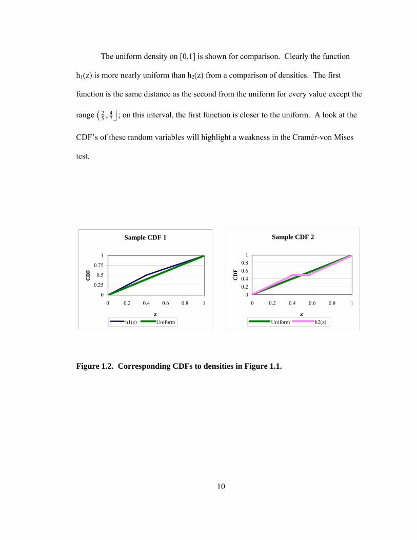
Figure 1.1. Two sample densities compared with the uniform distribution.

10

The uniform density on [0,1] is shown for comparison. Clearly the function

h1(z) is more nearly uniform than h2(z) from a comparison of densities. The first

function is the same distance as the second from the uniform for every value except the

range ( 2 45 7, ⎤⎦ ; on this interval, the first function is closer to the uniform. A look at the

CDF’s of these random variables will highlight a weakness in the Cramér-von Mises

test.

Sample CDF 1

0

0.25

0.5

0.75

1

0 0.2 0.4 0.6 0.8 1

z

CD

F

h1(z) Uniform

Sample CDF 2

00.20.40.60.8

1

0 0.2 0.4 0.6 0.8 1

z

CD

F

Uniform h2(z)

Figure 1.2. Corresponding CDFs to densities in Figure 1.1.

11

The CDF of h2(z) is the same distance from the 45° degree line as is h1(z)

everywhere except the interval ( 2 45 7, ⎤⎦ ; on this interval, its distance from the uniform is

smaller that the distance of h1(z). Thus, the integrated squared distance is smaller for

h2(z) than for h1(z). Therefore, the Cramér-von Mises test would be less likely to reject

h2(z) than h1(z) even though h2(z) departs more from the uniform. Since the

investigator is not likely to know the type of departure from the hypothesized

distribution a priori, it seems that a reasonable property for a GFT is to be more

sensitive to greater departures.

The best-known GFT is the Pearson χ2 test. It is safe to say that it appears in

more texts than any other GFT (See for example Hogg & Craig (1970)). For a

multinomial distribution with n observations the test is:

H0: pj = pj0 , j = 1, …, m+1 vs. H1: Not H0

The Pearson statistic is Qm = ( )2

1 0

01

m j j

jij

Obs np

np

+

=

⎡ ⎤−⎢ ⎥⎢ ⎥⎢ ⎥⎣ ⎦

∑ where Obsj is the number of

observations in the sample with the jth value.2 Any known distribution can be

transformed to a multinomial distribution with parameters {pj} by segmenting the

support of the distribution into m+1 sub-supports or “bins” and calculating the

population probability for each sub-support. It is not required that the pj be equal. This

statistic is easy to calculate, known to be asymptotically distributed as a χ2 statistic with

m degrees of freedom and can be used in a wide variety of situations. Its power is

dependent both on the choice of m and the choice of {pj}. It is intuitive that some 2 Here m+1 is used to facilitate future comparison with other tests. There are only m probability parameters being set since one of the parameters is constrained to be one minus the sum of the others.

12

power will be lost due to the reduction of information by grouping the data to test

continuous distributions. This grouping has the effect of assigning an equal density to

all possible values within each bin and also, perhaps, assigning nearby values that

happen to be in different bins very different density values. The following example will

highlight possible problems with this type of test.

Consider a test to determine whether n observations are from a standard normal

distribution with m + 1 = 10. For equiprobable bins, one would need 9 breakpoints

1

10j− ⎛ ⎞Φ ⎜ ⎟

⎝ ⎠, j = 1, …, 9, where Φ is the standard normal distribution. Below is a graph

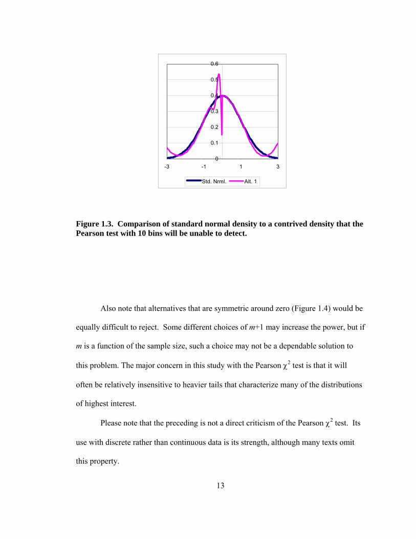
of a standard normal density and also a contrived density (Figure 1.3) that integrates to

½ on either side of zero; it also integrates to very close to 0.1 between consecutive

standard normal deciles. Consequently, a Pearson χ2 test could not tell the difference

between a normal distribution and the pictured alternative.

13

0

0.1

0.2

0.3

0.4

0.5

0.6

-3 -1 1 3

Std. Nrml. Alt. 1

Figure 1.3. Comparison of standard normal density to a contrived density that the Pearson test with 10 bins will be unable to detect.

Also note that alternatives that are symmetric around zero (Figure 1.4) would be

equally difficult to reject. Some different choices of m+1 may increase the power, but if

m is a function of the sample size, such a choice may not be a dependable solution to

this problem. The major concern in this study with the Pearson χ2 test is that it will

often be relatively insensitive to heavier tails that characterize many of the distributions

of highest interest.

Please note that the preceding is not a direct criticism of the Pearson χ2 test. Its

use with discrete rather than continuous data is its strength, although many texts omit

this property.

14

0

0.1

0.2

0.3

0.4

0.5

0.6

-3 -1 1 3

Std. Nrml. Alt. 2

0

0.1

0.2

0.3

0.4

0.5

0.6

-3 -1 1 3

Std. Nrml. Alt. 3

Figure 1.4. Additional densities that the Pearson test will be unable to detect.

1.4 PRESENCE OF ESTIMATED MODEL PARAMETERS

In most models the residuals are estimates of the unknown underlying errors.

Roughly speaking, one can visually assess and infer a distribution of error terms from a

histogram of residuals. However, a visual assessment should be reduced to a

mathematical assessment since histograms will necessarily differ from underlying

distributions and what is desired is a determination of whether or not the histogram in

question is statistically significantly different from the hypothesized theoretical

distribution. For this task, GFTs must be designed to meet the varying needs of each

situation.

15

In general, the error random variables to be tested are unobservable. With a

standard regression model:

yi = h(Xi;β )+ ε i (Eq. 1.3.1)

is assumed to be true with i = 1 , …, n, where yi is the ith observed dependent variable,

Xi is a row vector (with dimension k) of known constants (or is uncorrelated with the

vector of ε’s),3 β is a k-vector of unknown coefficients, and εi is an unobservable

random variable with some distribution, with E(εi) = 0 (or possibly the median of εi’s

distribution is zero), Pr(εi < z) = F(z;γ), γ ∈ Γ, and εi is independent of εj if i ≠ j. The

function h(Xi;β ) could be linear or non-linear.

Under these assumptions we would like to test whether the vector

ε = 1 nε ε′

⎡ ⎤⎣ ⎦L is distributed according to the given function or if it has some other

distribution. Typically, one must estimate β and γ, after which one can find a vector of

residuals (e) that is an estimate of ε, rather than ε itself. McCulloch (1999) reports the

fact that if parameters are to be estimated from the data, standard tests are biased

towards acceptance of the null hypothesis, citing Mood, Graybill & Boes (1974), Bera

and McKenzie (1986), and Bai (1997). He continues to convey that such tests “may

even be asymptotically invalid.” DeGroot (1986) reports that Chernoff and Lehmann

(1954) established that the use of maximum likelihood estimates, when testing whether

a given distribution is normal, changes the asymptotic distribution of the test statistic

under the null hypothesis in such a way as to result in smaller values. Given that larger

values are necessary to reject the null hypothesis, this results in a greater than desired

3 As usual, it is further assumed that the matrix composed of rows of the Xi’s is of rank k.

16

level of acceptance. Work completed in this dissertation provides empirical evidence to

support this for the application of stock market returns.

Intuitively, any “good” estimators of the parameters seek to fit the model as

closely as possible. For example, with a classical linear regression and leptokurtic

errors, the sum of the squared true errors will almost surely be greater than4 the sum of

the squared residuals. This will tend to conceal the large errors that a test for

leptokurtosis would be seeking.

Rayner and Best suggest a solution to the problem of testing for normality using

residuals of Eq. 1.3.1 for a classical linear model, with the error terms assumed to be

IID with the CDF given as N(0,σ2). First, start with your favorite goodness-of-fit

statistic (GFS), using the residuals. By taking advantage of the familiar result from

linear regression:

e = Mε , where M = I – X(X′X)-1X′ (Eq. 1.3.2)

it is possible to simulate several new sets of pseudo-residuals by generating random

variables from a standard normal distribution and multiplying these normal random

variates by M. Conveniently, the matrix M must be calculated only once for a given

model. It is unnecessary to estimate σ2 for most purposes unless the statistic chosen is

not invariant with respect to σ2. For each set of pseudo-residuals, calculate a GFS.

Thus, under an assumption of normality, you can form a Monte Carlo distribution for

the goodness-of-fit statistic. Use the distribution to determine a p-value for the original

GFS.

4 With a continuous error distribution, the probability is zero that the maximum likelihood estimates will, in fact, equal the true parameter values, so equality of the sums of squares has probability zero.

17

This method should be reasonable in many cases for its purpose, but some

difficulties exist. If the random errors are not independent and a variance matrix Ω is

known, M can be modified in the familiar way for generalized least squares. However,

generally Ω must be estimated complicating any interpretation between the ε vector and

the residuals. M has dimensions n × n and may be troublesome for especially large

databases. This procedure may not be able to be extended in a straightforward manner

to accommodate other situations that may arise such as non-linear regression or non-

Gaussian error terms. So, the search remains for suitable alternate tests.

18

CHAPTER 2

PRELIMINARIES IN THE DEVELOPMENT OF AN APPROPRIATE LAGRANGE MULTIPLIER TEST

2.1 LAGRANGE MULTIPLIER (LM) TEST5 FOR A UNIFORM DISTRIBUTION

Consider a random sample x = (x1, …, xn)′ from an unknown distribution F(X).

One would like to test:

H0: X ~ U(0,1) vs. H1: Not H0

One could parameterize the alternative hypothesis in the following way:

H1: X ~ G(z) where G(z) = ( )0

1

0 0

1 0 1

1 1

mzj j

j

z

v dv z

z

α φ=

<⎧⎪

⎡ ⎤⎪ + ≤ ≤⎢ ⎥⎨⎢ ⎥⎪ ⎣ ⎦

⎪ >⎩

∑∫ .

To assure that G(1) = 1, {φ j; j = 1, …,m} is chosen so each element, φ j, integrates to

zero on the unit interval. For the set of alternative hypotheses not to contain redundant

representations, {φ j; j = 1, …, m} must contain linearly independent elements.6 It will

also be convenient to require that φ j is bounded on the unit interval. With no additional

definition, the density associated with G can be written as: 5 Such tests are also called “efficient score” tests, just “score” tests, or sometimes “Rao score” tests in honor of the first to suggest this type of test. 6 As will be discussed later, any set of linearly independent functions that integrate to zero may be chosen which will be sensitive to possibly different departures with different power.

19

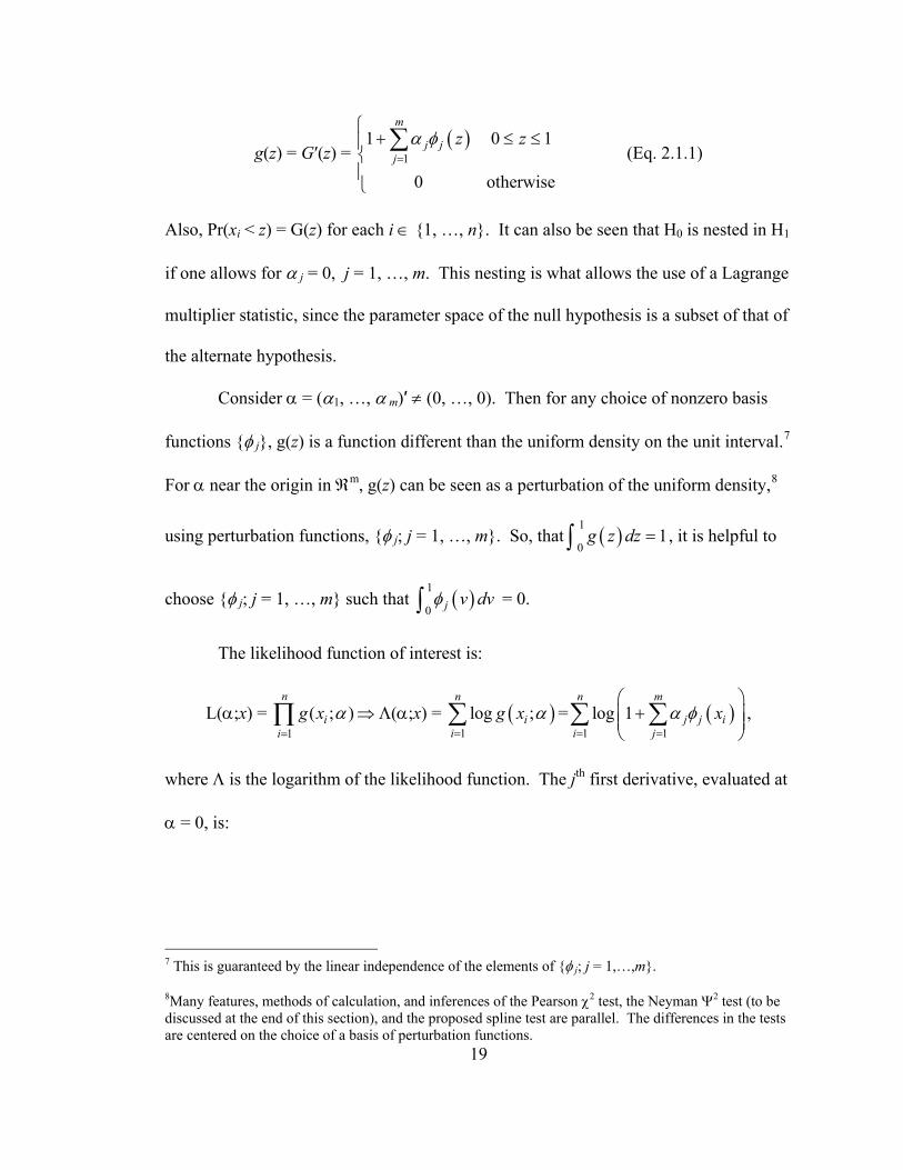
g(z) = G′(z) = ( )

11 0 1

0 otherwise

m

j jj

z zα φ=

⎧+ ≤ ≤⎪

⎨⎪⎩

∑ (Eq. 2.1.1)

Also, Pr(xi < z) = G(z) for each i ∈ {1, …, n}. It can also be seen that H0 is nested in H1

if one allows for α j = 0, j = 1, …, m. This nesting is what allows the use of a Lagrange

multiplier statistic, since the parameter space of the null hypothesis is a subset of that of

the alternate hypothesis.

Consider α = (α1, …, α m)′ ≠ (0, …, 0). Then for any choice of nonzero basis

functions {φ j}, g(z) is a function different than the uniform density on the unit interval.7

For α near the origin in ℜm, g(z) can be seen as a perturbation of the uniform density,8

using perturbation functions, {φ j; j = 1, …, m}. So, that ( )1

01g z dz =∫ , it is helpful to

choose {φ j; j = 1, …, m} such that ( )1

0 j v dvφ∫ = 0.

The likelihood function of interest is:

L(α;x) = 1

( ; )n

ii

g x α=

∏ ⇒ Λ(α;x) = ( )1

log ;n

ii

g x α=∑ = ( )

1 1log 1

n m

j j ii j

xα φ= =

⎛ ⎞+⎜ ⎟⎜ ⎟

⎝ ⎠∑ ∑ ,

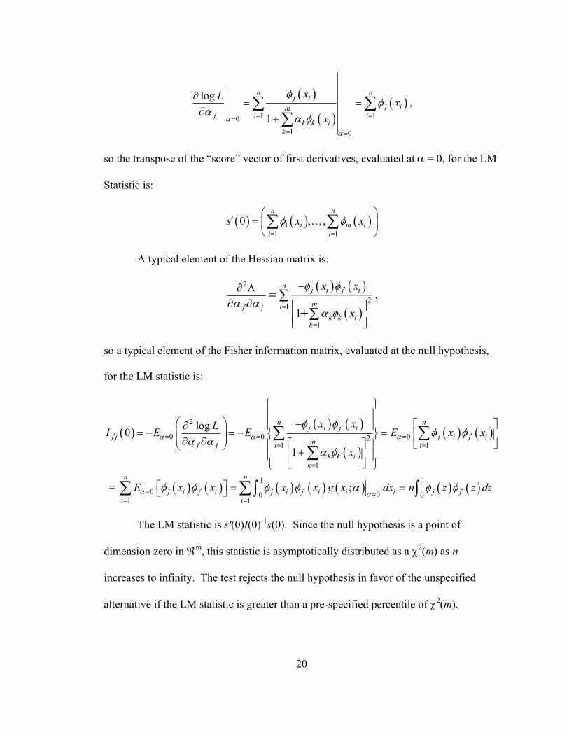
where Λ is the logarithm of the likelihood function. The jth first derivative, evaluated at

α = 0, is:

7 This is guaranteed by the linear independence of the elements of {φ j; j = 1,…,m}. 8Many features, methods of calculation, and inferences of the Pearson χ2 test, the Neyman Ψ2 test (to be discussed at the end of this section), and the proposed spline test are parallel. The differences in the tests are centered on the choice of a basis of perturbation functions.

20

( )

( )( )

1 10

1 0

log

1

n nj i

j imj i i

k k ik

xL xxα

α

φφ

αα φ= ==

= =

∂= =

∂+

∑ ∑∑

,

so the transpose of the “score” vector of first derivatives, evaluated at α = 0, for the LM

Statistic is:

( ) ( ) ( )11 1

0 , ,n n

i m ii i

s x xφ φ= =

⎛ ⎞′ = ⎜ ⎟

⎝ ⎠∑ ∑K

A typical element of the Hessian matrix is:

( ) ( )

( )

2

21

11

n j i j i

mij jk k i

k

x x

x

φ φα α

α φ

′

=′

=

−∂ Λ∂ ∂ ⎡ ⎤

⎢ ⎥⎣ ⎦

= ∑+∑

,

so a typical element of the Fisher information matrix, evaluated at the null hypothesis,

for the LM statistic is:

( ) ( ) ( )

( )( ) ( )

2

0 0 021 1

1

log0

1

n nj i j i

j j j i j imj j i i

k k ik

x xLI E E E x x

xα α α

φ φφ φ

α αα φ

′′ ′= = =

′ = =

=

⎧ ⎫⎪ ⎪

⎛ ⎞ − ⎡ ⎤⎪ ⎪∂= − = − =⎜ ⎟ ⎨ ⎬ ⎢ ⎥⎜ ⎟∂ ∂ ⎡ ⎤ ⎣ ⎦⎪ ⎪⎝ ⎠ +⎢ ⎥⎪ ⎪

⎣ ⎦⎩ ⎭

∑ ∑∑

= ( ) ( ) ( ) ( ) ( ) ( ) ( )1 1

0 00 01 1

;n n

j i j i j i j i i i j ji i

E x x x x g x dx n z z dzα αφ φ φ φ α φ φ′ ′ ′= =

= =

⎡ ⎤ = =⎣ ⎦∑ ∑∫ ∫

The LM statistic is s′(0)I(0)-1s(0). Since the null hypothesis is a point of

dimension zero in ℜm, this statistic is asymptotically distributed as a χ2(m) as n

increases to infinity. The test rejects the null hypothesis in favor of the unspecified

alternative if the LM statistic is greater than a pre-specified percentile of χ2(m).

21

The finite sample distribution for various values of n and m can be tabulated by

Monte Carlo simulation. For a given n, as m is increased, the power of the test relative

to specific alternative distributions was thought to increase, at least to a point. It was

anticipated that m should be an increasing function of n. McCulloch (1971, 1975)

suggests m ≈ n , whereas Li (1997) suggests m = an2/5. Simulations suggested that

different m were more appropriate for particular alternate hypotheses rather than

increasing with some power of n.

Two common estimators of the Fisher information matrix9 are the local

information matrix (the negative of the empirical Hessian of the log likelihood function)

and the Outer Product of the Gradient Estimator (OPG). Both estimators are consistent

estimators for the Fisher information matrix. A typical element of the local information

matrix is, evaluated at the null hypothesis is:

( ) ( )2

10

log n

j i j iij j

L x xα

φ φα α ′

=′ =

∂−

∂ ∂= ∑

The OPG estimator is also an empirical estimator. It is based on the

contributions to the gradient matrix, a typical element of which is:

( ) ( )0

log , ij i

j

L xx

α

αφ

α=

∂=

∂.

The typical element of the OPG matrix is:

( ) ( ) ( ) ( )1 10

log , log ,n ni i

j i j ij ji i

L x L xx x

α

α αφ φ

α α ′′= ==

∂ ∂=

∂ ∂∑ ∑ .

9 See for example Davidson and MacKinnon (1993) or McCulloch (1999)

22

Although in this case the estimators turn out to have the same form, that is not

always the case. In general, since the Hessian and the OPG depend on the sample rather

than the expectation, there is additional error included that inherently makes inferences

poorer than if the Fisher information matrix can be computed.

2.2 TECHNICAL CONSIDERATIONS

There are two technical points to discuss. The first of these is a requirement that

the parameter space for the null hypothesis is not on the boundary of the parameter

space for the alternative hypothesis (with the parameter space being defined as those

α that allow g to be a legitimate density).10 Intuitively, α = 0 is an interior point of the

parameter space, since at α = 0, g(z;α) = 1, for all values of z on the unit interval; and,

evidently, under the null hypothesis, there is a limiting local maximum at α = 0 as the

sample size increases to infinity. A more formal proof of the origin being an interior

point follows:

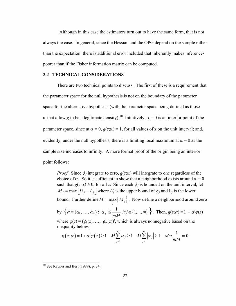
Proof. Since φ j integrate to zero, g(z;α) will integrate to one regardless of the choice of α. So it is sufficient to show that a neighborhood exists around α = 0 such that g(z;α) ≥ 0, for all z. Since each φ j is bounded on the unit interval, let

max ,j j jM U L⎡ ⎤= −⎣ ⎦ where Uj is the upper bound of φ j and Lj is the lower

bound. Further define { }max jjM M= . Now define a neighborhood around zero

by {α = (α1, …, αm) : { }1 , 1, ...,j j mmM

α ≤ ∀ ∈ }. Then, g(z;α) = 1 + α′ϕ(z)

where ϕ(z) = (φ1(z), …, φm(z))′, which is always nonnegative based on the inequality below:

( ) ( )1 1

1; 1 1 1 1 0m m

j jj j

g z z M M MmmM

α α ϕ α α= =

′= + ≥ − ≥ − ≥ − =∑ ∑

10 See Rayner and Best (1989), p. 34.

23

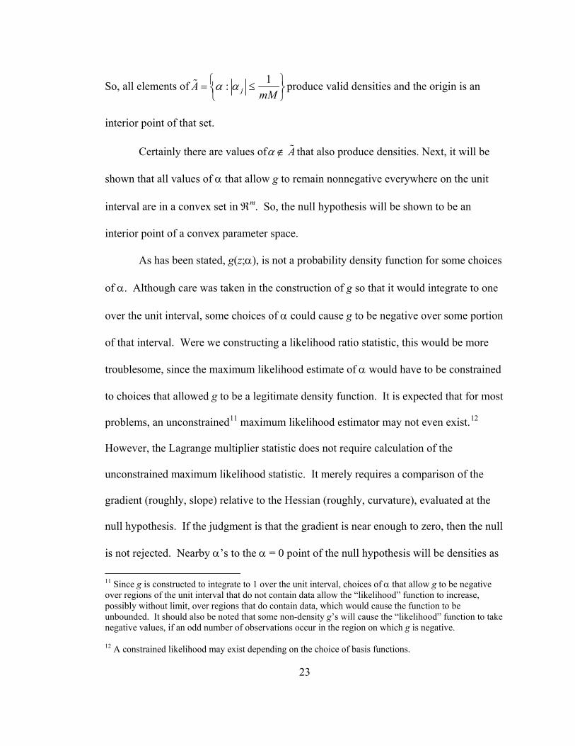
So, all elements of 1: jAmM

α α⎧ ⎫= ≤⎨ ⎬⎩ ⎭

% produce valid densities and the origin is an

interior point of that set.

Certainly there are values of Aα ∉ % that also produce densities. Next, it will be

shown that all values of α that allow g to remain nonnegative everywhere on the unit

interval are in a convex set in ℜm. So, the null hypothesis will be shown to be an

interior point of a convex parameter space.

As has been stated, g(z;α), is not a probability density function for some choices

of α. Although care was taken in the construction of g so that it would integrate to one

over the unit interval, some choices of α could cause g to be negative over some portion

of that interval. Were we constructing a likelihood ratio statistic, this would be more

troublesome, since the maximum likelihood estimate of α would have to be constrained

to choices that allowed g to be a legitimate density function. It is expected that for most

problems, an unconstrained11 maximum likelihood estimator may not even exist.12

However, the Lagrange multiplier statistic does not require calculation of the

unconstrained maximum likelihood statistic. It merely requires a comparison of the

gradient (roughly, slope) relative to the Hessian (roughly, curvature), evaluated at the

null hypothesis. If the judgment is that the gradient is near enough to zero, then the null

is not rejected. Nearby α’s to the α = 0 point of the null hypothesis will be densities as

11 Since g is constructed to integrate to 1 over the unit interval, choices of α that allow g to be negative over regions of the unit interval that do not contain data allow the “likelihood” function to increase, possibly without limit, over regions that do contain data, which would cause the function to be unbounded. It should also be noted that some non-density g’s will cause the “likelihood” function to take negative values, if an odd number of observations occur in the region on which g is negative. 12 A constrained likelihood may exist depending on the choice of basis functions.

24

will be shown more formally relative to the previous technical point addressed. In fact,

all the g(z;α) that are legal densities are near one another in the sense that the values of

α that allow g to remain nonnegative are in a convex set in ℜm.

Proof. Let α = (α1, …, αm)′ ∈ ℜm, ϕ(z) = (φ1(z), …, φm(z))′. Assume the contrary: at least one of the densities is not in a common convex region of ℜm. Then there must be at least one function g(z;ω) that becomes negative at some point z0 ∈ [0,1], such that ω is a convex combination13 of ξ and ζ, where g(z;ξ) and g(z;ζ) are nonnegative everywhere on the unit interval.14

So, g(z0; tξ + (1-t)ζ) = 1 + ( tξ + (1-t)ζ)′ϕ(z0) < 0 ⇒ tξ′ϕ(z0) + (1-t)ζ′ϕ(z0) < -1 Since g(z0;ξ) = 1 + ξ′ϕ(z0) ≥ 0 and g(z0;ζ) = 1 + ζ′ϕ(z0) ≥ 0, tξ′ϕ(z0) + (1-t)ζ′ϕ(z0) ≥ -t – (1-t) = -1, which is a contradiction.

So, the assumption that g(z;ω) becomes negative at some point z0 ∈ [0,1] is impossible

and, thus, the densities are in a convex region of ℜm.

2.3 SPLINE LAGRANGE MULTIPLIER TEST FOR A UNIFORM

DISTRIBUTION

It is required that ( )1

0 j v dvφ∫ = 0; one way of assuring this is to choose any set

of functions {ψj} that are integrable over [0,1] and with ψ j(z) = Ψj′(z), and define

φ j(z)= ψ j(z) - ( )1

0 j v dvψ∫ , since ( )1 1

0 0( )j jv u du dvψ ψ⎡ ⎤−⎢ ⎥⎣ ⎦∫ ∫ =

( ) ( ){ } 11

0 0

vuj j u v

v v u==

= =⎡ ⎤Ψ − Ψ⎣ ⎦ = Ψj(1) − [Ψj(1) − Ψj(0)] − Ψj(0) = 0 .

If we wanted to define a cubic spline, we could, for example, define

13 ω = tξ + (1-t)ζ for some t ∈ [0,1] 14 ω,ξ, and ζ are all choices of α ∈ ℜm

25

( ) 3

1, 2

3max , 0 3, 4, ,2

j

j

z j

z jz j mm

ψ

⎧ =⎪⎪ ⎧ ⎫= ⎨ −⎪ ⎪⎛ ⎞− =⎨ ⎬⎜ ⎟⎪ −⎝ ⎠⎪ ⎪⎪ ⎩ ⎭⎩

K.

The bottom functional form can be visualized as translating the function z3+, such that

its origin is at each of the set of points {0, (m-2)-1, 2(m-2)-1, …, (m-3) (m-2)-1}, where

33 0

0 0z zz

z+ ⎧ ≥⎪= ⎨

<⎪⎩, the positive portion of z3.

The value, first derivative and second derivative of the ψ j’s are zero at 23

−−

mj , where

the positive portion of the function begins; so, the addition of a multiple of ψ j to a

cubic function (or to a different cubic spline) results in a cubic spline. Thus, this set of

ψ j’s form a basis for cubic splines with equidistant knots on [0,1].15

It appears that, using the cubic spline basis, the Fisher information matrix can be

calculated directly, so reliance on estimates in this case is unnecessary. The φ’s that are

in the integrand of the typical element of this Fisher information matrix are cubic

polynomials over part of their range and constant functions over the other part. So, it is

only necessary to integrate zero-degree, cubic and sextic polynomials. Thus, we must

evaluate linear, quartic and septemic polynomials at zero, one, and all knotpoints.

Some benefits and concerns of this type of basis will be presented in the next chapter.

There is nothing a priori to compel the selection of cubic splines instead of

quadratic or linear splines. In fact even an exponentiated spline, using expressions of 15 A spline is a function of a given number m of piecewise polynomials (or some other general function) of a given degree n, each defined on a subset of a range, connected at m-1 points in the range, called nodes or knots, such that the values and derivatives up to degree m-1 of consecutive polynomials are identical at the nodes. Thus, cubic splines require values and first and second derivatives of consecutive cubic polynomials to be equal at the knots.

26

the form “ ( )exp j jα φ ” in the alternative hypothesis, may be a reasonable basis for a

test.16 Quadratic and cubic splines are more aesthetic than linear splines in constructing

likely alternative densities in that their knots are not discernible since the first

derivatives of contiguous polynomials are equal. Cubic splines perhaps are to be

preferred to quadratic splines since they are allowed to bend twice in a subinterval so

they may be better at imitating the tails of some alternative distributions, but that

characteristic may be at the expense of some other desired feature.

At this point, it can be noted that the Pearson χ2 test is equivalent to a zero-

degree spline GFT for a continuous distribution. Recall the structure of the hypotheses:

H0: pj = pj0 , j = 1, …, m+1 vs. H1: Not H0

If each of the pj0 is set to a constant p, then H0 becomes the uniform discrete

distribution. So a random sample, x = (x1, …, xn)′ from an unknown distribution F(X)

can be tested using:

H0: X ~ U(0,1) vs. H1: X ~ G(z)

where g(z) can be of the form of equation Eq. 2.1.1, H1:17

16 Please see Appendix E for a proof that the proposed LM statistic is invariant to linear combinations and exponentiation of basis functions, regardless of whether the basis functions are polynomials, splines, or some other bounded function. 17 There are alternative representations as well, with one being:

g(z) = ( )1

1m

k kk

zα φ=

+ ∑ , where, ( ) [ ]1

11

,, 1, ,

10 0,1

otherwise

k km m

k

m

k mz

z zφ

−

−

⎧ ⎡ ⎤⎣ ⎦⎪=⎨

⎪⎩

∈= ∉

−K

27

g(z) = ( )1

1m

k kk

zα φ=

+ ∑ , where, ( ))1

1 1

1

1 ,

1 ,1 , 1, ,

0 otherwise

k km m

mk m

z

z z k mφ

−+ +

+

⎧ ⎡∈ ⎣⎪⎪ ⎡ ⎤= − ∈ =⎨ ⎣ ⎦⎪⎪⎩

K .

This zero-degree spline Lagrange multiplier test statistic (ZSLM) would be formed in

the same way as that of the cubic spline Lagrange multiplier test statistic (CSLM), by

using the score vector and Fisher information matrix indicated by the log likelihood

function.

The score evaluated at the null hypothesis is:

( ) ( ) ( )11 1

0 , ,n n

i m ii i

s x xφ φ= =

⎛ ⎞′ = ⎜ ⎟

⎝ ⎠∑ ∑K ,

a typical element of which would be (nj - nm+1), where nj is the number of observations

in the jth bin, or in the interval [ 11 1,j j

m m−+ + ) and nm+1 is the number of observations in the

last bin, or in the interval [ 1 ,1mm+ ].

A typical element of the Fisher information matrix is

( ) ( ) ( )1

00j j j jI n z z dzφ φ′ ′= ∫ ,

so diagonal elements are 21

nm+ and off-diagonal elements are 1

nm+ . Such a matrix is easy

to invert, with the inverse’s diagonal elements being mn and the off-diagonal elements

equal to 1n− .

2.4 B-SPLINE BASIS

Although the theoretical choice of a basis allows for any set of linearly

independent bounded functions, there are numerical considerations in choosing a basis

28

so that reasonable results can be obtained. The simple cubic spline basis pictured below

with seven members has a Fisher information matrix that is poorly conditioned for

inversion for large m. The seventh member is barely visible ranging from a minimum

value of -0.0004 to a maximum of 0.0076 which would necessitate that its coefficient

might be 2 to 3 orders of magnitude greater than a coefficient from one of the first few

basis members. The difference in magnitude increases greatly as m increases.

-0.5

-0.25

0

0.25

0.5

0.75

0 0.2 0.4 0.6 0.8 1

Figure 2.1. Simple cubic spline basis vectors for m=7

29

Another basis for splines, typically called B-splines,18 and the one that is used in

the new Lagrange multiplier test, is presented below; it is visually shown in Figure 2.2.

It has the advantage that all the basis members are of the same order of magnitude and

the Fisher information matrix will be dominated by a strong diagonal and be nearly

sparse. Using B-splines, the linear spline matrix will be nearly tridiagonal, the

quadratic spline matrix will have larger values on the main diagonal plus the four

diagonals nearest the main diagonal, while the cubic spline matrix will have its largest

values on the seven main diagonals. As such, this choice of bases is much better

conditioned for inversion of Fisher information matrices and for accumulating the

corresponding scores.

In general, B-splines of order k (k=1 corresponding to linear splines, k=2

corresponding to quadratic splines, k=3 corresponding to cubic splines, and so on)

require k+1 basis functions for the first segment, with the requirement of adding one

basis function for each additional segment. However, the splines that we are interested

in have a requirement of integrating to zero over the unit interval. Consequently, we

can construct the splines with one fewer basis function.

Linear B-spline functions look like “tent” functions increasing linearly from

zero to a maximum from one knot point to the next, then decreasing from that

maximum back to zero. Since this application requires the functions to integrate to zero

on [0,1], these “tents” will be translated downward so that some of their range will be

negative.

18 See Judd, p. 227

30

The functional form for the linear spline basis with m equal segments (and m+1

knots) is shown below. Superscripts of “1” will distinguish these basis functions from

the quadratic spline basis functions, which have a superscript of “2” and the cubic

spline basis functions which have a superscript of “3”:

( ) ( )1 1 1, 0,1, , 1i i ix x c i mφ ψ= − = −K , where

( )1

1 2 1 2

ifif

0 otherwise

i i im m m

i i ii m m m

x xx x xψ

+

+ + +

⎧ − ≤ ≤⎪= − ≤ ≤⎨⎪⎩

and{ }2

2

11

12

if 0,1, , 2

if 1m

im

i mc

i m

⎧ ∈ −⎪= ⎨= −⎪⎩

K.

It must be understood that the functions need not be defined outside the unit interval.

For ease of exposition, that contingency is ignored. For example, the second segment

of ψm-11 by the above definition is defined on the interval [1, (m+1)/m] but is

unnecessary for this application.

If the segments are unequal in length, one can substitute {x0 , x1 , …, xm} for

{ }0,1, ,im i m= K as boundaries for the various domain segments in the above formula,

where x0 and xm substitute for zero and one, respectively, while x1, x2, …, xm-1 are the

desired knot points.

The formula for quadratic splines is a bit more complicated with three non-

trivial expressions defining each basis function. In addition, there must be one more

function than in the basis for the linear spline to produce the same number of

polynomial segments in the quadratic spline; so with m basis functions, one can

describe only m-1 quadratic segments and m-2 knots.

( ) ( )2 2 2 , 1, 0,1, , 2i i ix x c i mφ ψ= − = − −K , where

31

( )

( )( ) ( ) ( ) ( )

( )

2 11 1 1

2 3 1 1 21 1 1 1 1 12

23 2 31 1 1

if

if

if

0 otherwise

i i im m m

i i i i i im m m m m m

ii i im m m

x x

x x x x xx

x xψ

+− − −

+ + + + +− − − − − −

+ + +− − −

⎧ − ≤ ≤⎪⎪ − − + − − ≤ ≤⎪= ⎨⎪ − ≤ ≤⎪⎪⎩

and

( )

( ){ }

( ){ } { }

( )

( )

3

3

3

3

3

43 1

53 1

623 1

53 1

13 1

if 1& 1 1

if 1& 1 2,3,

if 0,1, , 4 & 1 3, 4,

if 0 & 3

if 2

m

m

i m

m

m

i m

i m

i m mc

i i m

i m

−

−

−

−

−

⎧ = − − =⎪⎪ = − − ∈⎪⎪ ∈ − − ∈= ⎨⎪

≥ = −⎪⎪

= −⎪⎩

K

K K .

The formula for cubic splines has four non-trivial expressions defining each

basis function. The m basis functions describe m-2 cubic segments and the

corresponding m-3 knots.

( ) ( )3 3 3, 2, 1, 0,1, , 3i i ix x c i mφ ψ= − = − − −K , where

( )

( )( ) ( ) ( )( )( ) ( )( )( )( ) ( )( )( ) ( ) ( )

( )

3

3 12 2 2

2 22 3 1 4 1 1 22 2 2 2 2 2 2 2 2

2 23 4 1 3 4 2 2 32 2 2 2 2 2 2 2 2

34 3 42 2

if

if

if

if

i

i i im m m

i i i i i i i i im m m m m m m m m

i i i i i i i i im m m m m m m m m

i i im m m

x

x x

x x x x x x x x

x x x x x x x x

x x

ψ

+− − −

+ + + + + + +− − − − − − − − −

+ + + + + + + +− − − − − − − − −

+ + +− − −

=

− ≤ ≤

− − + − − − + − − ≤ ≤

− − + − − − + − − ≤ ≤

− ≤ ≤ 2

0 otherwise

⎧⎪⎪⎪⎪⎨⎪⎪⎪⎪⎩

32

and

( ){ }

( ){ }

( )

( ){ }

( ){ } { }

( )

( )

( )

4

4

4

4

4

4

4

4

114 2

124 2

224 2

234 22

244 2

234 2

124 2

14 2

if 2, 1 & 2 1

if 2 & 2 2,3,

if 1& 2 2

if 1& 2 3, 4,

if 0,1, , 6 & 2 4,5,

if 0 & 5

if 0 & 4

if 3

m

m

m

mi

m

m

m

m

i m

i m

i m

i mc

i m m

i i m

i i m

i m

−

−

−

−

−

−

−

−

⎧ ∈ − − − =⎪⎪ = − − ∈⎪⎪ = − − =⎪⎪ = − − ∈⎪⎪= ⎨

∈ − − ∈⎪⎪

≥ = −⎪⎪⎪ ≥ = −⎪⎪ = −⎪⎩

K

K

K K.

-0.015

-0.01

-0.005

0

0.005

0.01

0.015

0.02

0.025

0.03

0 0.1 0.2 0.3 0.4 0.5 0.6 0.7 0.8 0.9 1

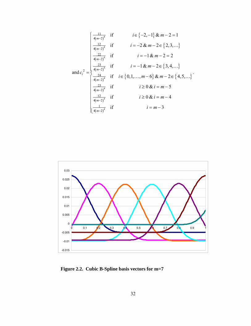
Figure 2.2. Cubic B-Spline basis vectors for m=7

33

Figure 2.2 is an illustration of a seven-function basis for cubic B-splines. Note

that there are 3 pairs of mirror-image functions and a function that is a bit below zero on

[0,0.8] and rising cubically on [0.8,1].

Starting from the left, the first and sixth basis functions contain only two cubic

segments (not including the constant segment). The second and fifth functions contain

three cubic segments, the third and fourth functions are the only ones that contain all

four cubic segments, while the seventh function contains only one cubic segment.

2.5 NEYMAN’S SMOOTH TEST

A GFT to which the CSLM is also closely related would be Neyman’s smooth

test.19 Smooth tests were so named because the alternative distributions varied

“smoothly” away from the null hypothesized distribution. Neyman called this test a Ψ2

test (which can be contrasted with Pearson’s χ2 test). Neyman constructed an

alternative hypothesis of order m (to a null of a uniform random variable on [0,1] ) to be

( ) ( ) ( )1

; expm

m j jj

g z K zα α α π=

⎧ ⎫⎪ ⎪= ⎨ ⎬⎪ ⎪⎩ ⎭∑ , 0 ≤ z ≤ 1, m = 1,2,…

where K(α) is the constant necessary for gm to be a density, and the πj are orthonormal

polynomials of degree j that integrate to zero on the unit interval. As in the general

case, the null hypothesis is that α = 0. With the exponentiation, there is no problem

with gm(z;α) taking negative values. We can reparameterize Neyman’s alternative as

19 See Rayner and Best (1989), p.7 and p.46-48. The choices of indices, variable and parameter names have been changed to show the parallel with the CSLM and ZSLM.

34

gm(z;α) = ( )

( )

1

1

01

exp 1

exp 1

m

j jj

m

j jj

z

z dz

α π

α π

=

=

⎧ ⎫⎪ ⎪+⎨ ⎬⎪ ⎪⎩ ⎭⎧ ⎫⎪ ⎪+⎨ ⎬⎪ ⎪⎩ ⎭

∑

∑∫, 0 ≤ z ≤ 1, m = 1,2,…

With this parameterization, the integral in the denominator is a constant depending on

the α vector of which can be represented by C(α) = ( )e

K α . Neyman’s test statistic is

Ψ2m=

( )2

1 1where

m nj i

j jj i

yU U

n

π

= =

=∑ ∑ . This test statistic is asymptotically χ2(m) .

Neyman expected that values of m of 4 or 5 would be sufficient to test a large enough

class of alternatives. Ψ2m was a likelihood ratio test statistic rather than a Lagrange

multiplier statistic. Since Neyman thought an m of 4 or 5 would be sufficient, it was not

necessary in practice to compute K(α) for larger values of m. To change this to a

Lagrange multiplier test with possibly larger values of m, which is concerned with

perturbations only in the neighborhood of the null hypothesis, it will be convenient to

simplify calculations by substituting a regular polynomial form in place of Neyman’s

exponentiated polynomial.

Using this structure, one definition could be:

g(z) = ( )1

1m

j jj

zα φ=

+ ∑ , where, ( ) [ ]11 0,1

0 otherwise

jj

jz z

zφ +⎧ − ∈⎪= ⎨⎪⎩

.

The corresponding LM test statistic, which is identical to an LM test statistic based on

an exponentiation, is formed in the same way as shown in Chapter 2.1, by using the

score vector and Fisher information matrix indicated by the log likelihood function:

35

Score: ( ) ( ) ( )11 1

0 , ,n n

i m ii i

s x xφ φ= =

⎛ ⎞′ = ⎜ ⎟

⎝ ⎠∑ ∑K , a typical element of which would be

1 1

nj

ii

nxj=

−+∑ . A typical element of the Fisher information matrix is

( ) ( ) ( )1

00j j j jI n z z dzφ φ′ ′= ∫ , or

1 1 11 10

( )( )( 1)( 1)( 1)

j jj j

njjn z z dzj j j j

′′+ +

′− − =

′ ′+ + + +∫ .

One difference between the CSLM test and Neyman’s test is that the CSLM is

more sensitive to differences that are local to a specific part of the unit interval.

Because Neyman’s exponentiated polynomials were defined over the entire interval,

each polynomial affected the likelihood of every data point. For this reason,

polynomials have to make compromises since, in order to fit one point better, it may be

necessary to fit other points that are not nearby more poorly. Splines are more pliable

and better able to fit points in a particular interval without affecting more distant

intervals as much. Additionally, higher-powered polynomials are computationally more

troublesome because of significant rounding errors when adding together terms with

greatly varying orders of magnitude between their coefficients.

“Experience with polynomials derived by truncating [Taylor]20 series[, especially in their use with estimating transcendental functions,] may mislead one into thinking that the use of high order polynomials does not lead to computational difficulties. However it must be appreciated that truncated [Taylor] series are not typical of polynomials in general. [Truncated Taylor series] have the special feature that the terms decrease rapidly in size for values of x in the range for which they are appropriate. A tendency to underestimate the difficulties involved in working with general polynomials is perhaps a consequence of one’s experience in classical analysis. There it is natural to regard a polynomial as a very desirable function since it is bounded in any finite region and has derivatives of all orders. In numerical work, however, polynomials having

20 Text uses the term “power” instead of Taylor

36

coefficients which are more or less arbitrary are tiresome to deal with by entirely automatic procedures.”21

Although there is more initial work to calculating and understanding splines,

they have some numerical properties that are more desirable than polynomials while the

tradeoff in the other properties is not severe. Splines retain the polynomial properties of

being bounded in any finite region and have derivatives of all orders at all points

excluding the relatively small finite number of knotpoints. Other concerns about

rounding are contained in Appendix G.

The Pearson, Neyman, and spline tests are all meet the criteria of the Neyman-

Pearson lemma against simple alternatives. So, it is expected that each test will work

better for alternatives that are of the form determined by their respective perturbing

functions. Tests with other bases of perturbing functions should be better for still other

distributions.

2.6 SIMPLE POLYNOMIAL BASIS

For practical computations with most software using double precision with 32-

bit processors, a basis of simple restricted polynomials, {xm – (m + 1)-1}, m = 1,2, …,

will likely be difficult to work with as m increases since the rows of the Fisher

information matrix are nearly linearly dependent.

It is very easy to compute the cells of such matrices. Each cell is

( ) ( ) ( )1 1 1ij

i j i j+ + + + where i is the row index and j is the column index. However,

21 Wilkinson, J. H., Rounding Errors in Algebraic Processes, p.38

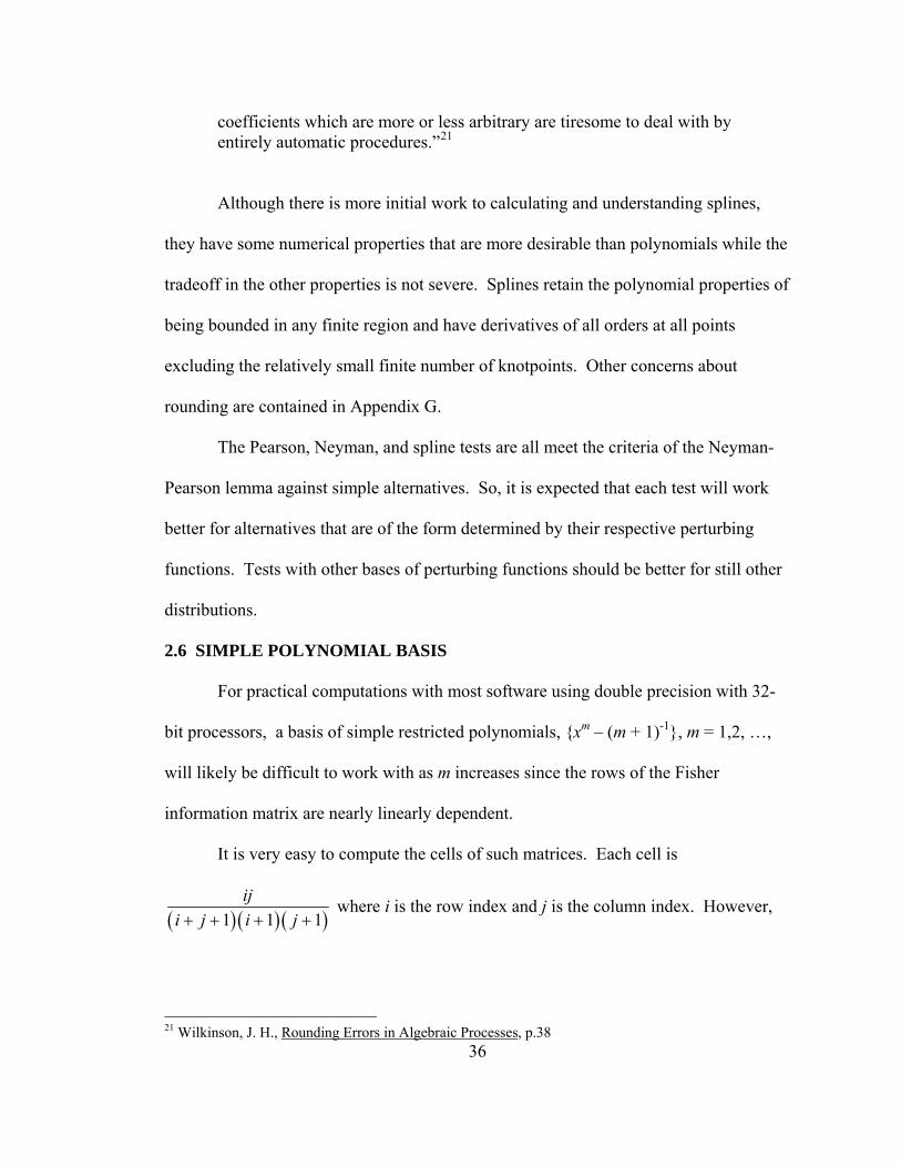
37

the determinants of the first 12 such matrices show that ill-conditioning occurs quite

rapidly and accelerates even faster:

M 1 2 3 4 5 6 Det 8.33e-02 4.63e-04 1.65e-07 3.75e-12 5.37e-18 4.84e-25

M 7 8 9 10 11 12

Det 2.73e-33 9.72e-43 2.16e-53 3.02e-65 2.64e-78 1.44e-92

Figure 2.3. Determinants of Fisher information matrices from first 12 simple polynomial bases

The first and third rows indicate the number of columns (and rows) in the

matrices and the second and fourth rows show the determinants. The determinant is

getting ever smaller at a faster and faster rate. So, the hope of obtaining meaningful

numerical inverses with conventional precision beyond the first few matrices is bleak.

A closer look at the 8 × 8 matrix shows two characteristics of these matrices: a

non-dominant main diagonal and rows that are nearly multiples of one another.

38

0.0833 0.0833 0.0750 0.0667 0.0595 0.0536 0.0486 0.04440.0833 0.0889 0.0833 0.0762 0.0694 0.0635 0.0583 0.05390.0750 0.0833 0.0804 0.0750 0.0694 0.0643 0.0597 0.05560.0667 0.0762 0.0750 0.0711 0.0667 0.0623 0.0583 0.05470.0595 0.0694 0.0694 0.0667 0.0631 0.0595 0.0561 0.05290.0536 0.0635 0.0643 0.0623 0.0595 0.0565 0.0536 0.05080.0486 0.0583 0.0597 0.0583 0.0561 0.0536 0.0510 0.04860.0444 0.0539 0.0556 0.0547 0.0529 0.0508 0.0486 0.0465

⎡ ⎤⎢ ⎥⎢⎢⎢⎢⎢⎢⎢⎢⎢⎢⎣ ⎦

⎥⎥⎥⎥⎥⎥⎥⎥⎥⎥

This suggests the topic of the next section: If a simple basis does not work, why not try

an orthogonal one?

2.7 ORTHOGONAL POLYNOMIAL BASIS

Alternatively, one can search for orthogonal polynomials so that the Fisher

information matrix is diagonal with an uncomplicated inverse. A recursive formula for

Legendre-type polynomials is shown below. The Legendre polynomials are typically

defined on the range [-1,1], so a change of variable is necessary so that the resultant

polynomials are orthogonal on our range of interest, [0,1].

Let p0(x) = 1 and p1(x) = 2x – 1. Then a recursive formula which will generate

as many orthogonal polynomials as necessary on [0,1] is:

pm+1 = [(2m + 1)(2x – 1) pm(x) – m pm-1(x)] / (m + 1), m = 1,2, …,

with ( )21

0

12 1mp x dx

m⎡ ⎤ =⎣ ⎦ +∫ , while, as designed, ( ) ( )1

00, if .m kp x p x dx m k⎡ ⎤ ⎡ ⎤ = ≠⎣ ⎦ ⎣ ⎦∫

The first few such polynomials are:

p0(x) = 1

p1(x) = 2x – 1

p2(x) = 6x2 - 6x + 1

39

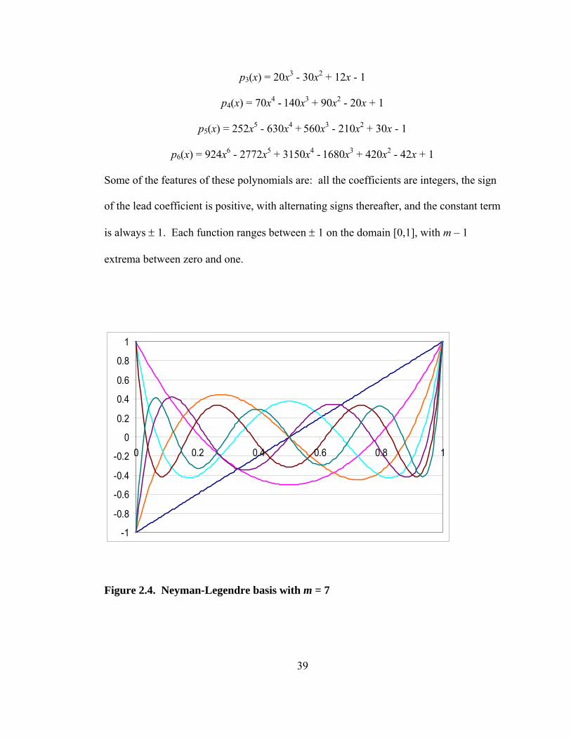
p3(x) = 20x3 - 30x2 + 12x - 1

p4(x) = 70x4 - 140x3 + 90x2 - 20x + 1

p5(x) = 252x5 - 630x4 + 560x3 - 210x2 + 30x - 1

p6(x) = 924x6 - 2772x5 + 3150x4 - 1680x3 + 420x2 - 42x + 1

Some of the features of these polynomials are: all the coefficients are integers, the sign

of the lead coefficient is positive, with alternating signs thereafter, and the constant term

is always ± 1. Each function ranges between ± 1 on the domain [0,1], with m – 1

extrema between zero and one.

-1

-0.8

-0.6

-0.4

-0.2

0

0.2

0.4

0.6

0.8

1

0 0.2 0.4 0.6 0.8 1

Figure 2.4. Neyman-Legendre basis with m = 7

40

The illustration above shows the first seven members of the Neyman-Legendre

type basis. Although now the Fisher information matrix is easy to compute, the other

component of the Lagrange multiplier statistic, the score, can become problematic

numerically as m increases because the relative magnitudes of the coefficients of the

polynomials grows very rapidly. As an example, for m = 24, the coefficients of the 13th

through 21st powers of x are on the order of 1016, whereas the constant term still has a

coefficient on the order of 100. Since most software carries only 16 significant digits in

its calculations, even with the use of Horner’s rule of polynomial evaluation,22 the

score, which is the sum of a number (equal to the sample size) of such polynomial

evaluations can be expected to pick up some significant errors for large m.

However, one can still obtain reasonable numerical results for values of m

beyond that which are obtainable with the simple polynomial basis.

22The evaluation of a standard polynomial, pm(x) = cmxm + … + c1x + c0 by successive multiplications instead of exponentiation: ((…(cmx + cm-1) x + cm-2) x + … + c1) x + c0

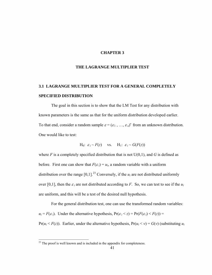
41

CHAPTER 3

THE LAGRANGE MULTIPLIER TEST

3.1 LAGRANGE MULTIPLIER TEST FOR A GENERAL COMPLETELY

SPECIFIED DISTRIBUTION

The goal in this section is to show that the LM Test for any distribution with

known parameters is the same as that for the uniform distribution developed earlier.

To that end, consider a random sample ε = (ε 1 , …, ε n)′ from an unknown distribution.

One would like to test:

H0: ε i ~ F(z) vs. H1: ε i ~ G(F(z))

where F is a completely specified distribution that is not U(0,1), and G is defined as

before. First one can show that F(ε i) = ui, a random variable with a uniform

distribution over the range [0,1].23 Conversely, if the ui are not distributed uniformly

over [0,1], then the ε i are not distributed according to F. So, we can test to see if the ui

are uniform, and this will be a test of the desired null hypothesis.

For the general distribution test, one can use the transformed random variables:

ui = F(ε i). Under the alternative hypothesis, Pr(ε i < z) = Pr(F(ε i) < F(z)) =

Pr(ui < F(z)). Earlier, under the alternative hypothesis, Pr(ui < v) = G(v) (substituting ui

23 The proof is well known and is included in the appendix for completeness.

42

for xi and v for z), where G is the same G as defined in Chapter 2.1. So, Pr(ε i < z) =

Pr(ui < F(z)) = G(F(z)).

The density associated with G(F(z)) is g(F(z))f(z), by the chain rule, where

g(z) = ( )1

1m

j jj

zα φ=

+ ∑ and f = F′. The likelihood and log-likelihood functions are:

L(α;ε) = ( )1

( ; )n

i ii

g u fα ε=

∏ ⇒ Λ(α;ε) = ( ) ( )1

log ;n

i ii

g u fα ε=∑

= ( ) ( )1 1

log ; logn n

i ii i

g u fα ε= =

+∑ ∑ .

Since the second summation is constant relative to α, the first and second

derivatives necessary to calculate the LM statistic are identical to those of the test for

the uniform distribution. Thus, one can simply use the transformed observations, F(ε i),

with the test for the uniform distribution. All tables and critical values that are suitable

for the test of uniformity are also suitable for a general distribution.

3.2 FINITE SAMPLE PROPERTIES WITH A COMPLETELY SPECIFIED

DISTRIBUTION

The Lagrange multiplier statistic has a limiting asymptotic distribution that is

chi-squared with degrees of freedom equal to m, the number of perturbation parameters.

Preliminary simulations suggested that for n ≥ 30 (sample size), m ≥ 5, and level of

significance = 0.05, the convergence to the limiting distribution is quite rapid. At the

alluded values of m, n, and test size, the 95th percentile of the simulated distributions

could not be distinguished from the 95th percentile of a chi-squared random variable. If

43

a lower level of significance is required, a higher sample size will be needed to use the

chi-square approximation.

Pearson Size Distortion (m=6)

-0.04

-0.03

-0.02

-0.01

0

0.01

0.02

0.03

0.04

0 0.1 0.2 0.3 0.4 0.5 0.6 0.7 0.8 0.9 1Cumulative Probability

Diff

eren

ce

n=30 n=100 n=300 n=1000 Upper Lower

`

Figure 3.1. Size distortion of Pearson test; difference between chi-square distribution and empirical distribution

44

Figure 3.1 shows some results from a simulation with 9999 repetitions.24 There

is not much size distortion even for relatively small sample sizes and virtually

undetectable distortion for n ≥ 300. The dashed line that appears ellipse-like indicates

95% upper and lower confidence limits of where a cumulative empirical distribution of

random draws from the chi-square distribution would be expected to lie. Since there

were 9999 repetitions, the equation for the confidence limits is:

Upper and Lower( )1

Confidence Limits = 1.969999

p p−± .

Differences for sample sizes of 30 and 100 appear jagged and non-distortion

free. In large part this is due to the empirical Pearson statistic having a discrete

distribution, which is being compared to the continuous chi-square distribution. When

n ≥ 300, even the discreteness of the Pearson statistic is not enough to cause differences

from the chi-square distribution that are significantly different than zero.

A nice feature shown in Figure 3.2 is that the size distortion is even lower in the

tail of the distribution, which is the focus of hypothesis testing.

24 In this study the number of simulation repetitions is consistently chosen to be 10h-1 where h is an integer, rather than 10h, so that the size (Type I error) of the tests that use the simulated results will be more accurate. Then for a given size (ξ), assuming that 10h(1- ξ) is an integer, the order statistic with the index 10h(1-ξ) can be used as the critical value. We could use 10h instead and interpolate between the integers immediately above and below (10h+1)(1-ξ) to get to the mixed number (10h+1)(1-ξ). However, this involves one more calculation. It also involves an assumption that the c.d.f., which may be unknown, is linear, at least near where the critical order statistics are expected to be. Although the difference from linearity may be slight if the number of simulations is great enough, it is not necessary to make such an assumption with the proper selection of the number of repetitions.

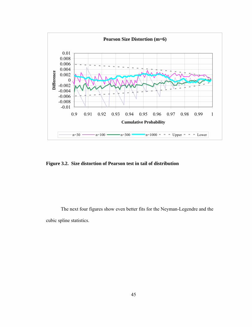
45

Pearson Size Distortion (m=6)

-0.01-0.008-0.006-0.004-0.002

00.0020.0040.0060.0080.01

0.9 0.91 0.92 0.93 0.94 0.95 0.96 0.97 0.98 0.99 1

Cumulative Probability

Diff

eren

ce

n=30 n=100 n=300 n=1000 Upper Lower

Figure 3.2. Size distortion of Pearson test in tail of distribution

The next four figures show even better fits for the Neyman-Legendre and the

cubic spline statistics.

46

Neyman Size Distortion (m=6)

-0.02

-0.01

0

0.01

0.02

0.03

0.04

0 0.1 0.2 0.3 0.4 0.5 0.6 0.7 0.8 0.9 1Cumulative Probability

Diff

eren

ce

n=30 n=100 n=300 n=1000 Upper Lower

`

Figure 3.3. Size distortion of Neyman-Legendre test; difference between chi-square distribution and empirical distribution

47

Neyman Size Distortion (m=6)

-0.01-0.008-0.006-0.004-0.002

00.0020.0040.0060.0080.01

0.9 0.91 0.92 0.93 0.94 0.95 0.96 0.97 0.98 0.99 1Cumulative Probability

Diff

eren

ce

n=30 n=100 n=300 n=1000 Upper Lower

Figure 3.4. Size distortion of Neyman-Legendre test in tail of distribution

48

Cubic Spline Size Distortion (m=6)

-0.02

-0.01

0

0.01

0.02

0.03

0.04

0 0.1 0.2 0.3 0.4 0.5 0.6 0.7 0.8 0.9 1Cumulative Probability

Diff

eren

ce

n=30 n=100 n=300 n=1000 Upper Lower

`

Figure 3.5. Size distortion of Cubic Spline test; difference between chi-square distribution and empirical distribution

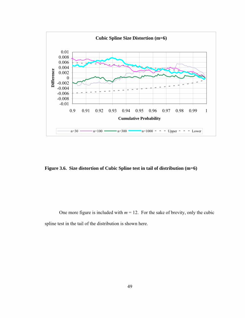
49

Cubic Spline Size Distortion (m=6)

-0.01-0.008-0.006-0.004-0.002

00.0020.0040.0060.0080.01

0.9 0.91 0.92 0.93 0.94 0.95 0.96 0.97 0.98 0.99 1

Cumulative Probability

Diff

eren

ce

n=30 n=100 n=300 n=1000 Upper Lower

Figure 3.6. Size distortion of Cubic Spline test in tail of distribution (m=6)

One more figure is included with m = 12. For the sake of brevity, only the cubic

spline test in the tail of the distribution is shown here.

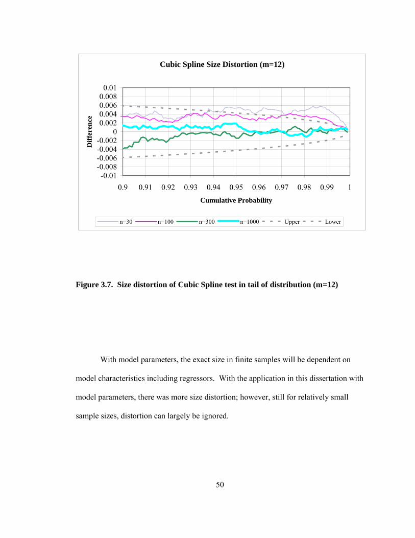
50

Cubic Spline Size Distortion (m=12)

-0.01-0.008-0.006-0.004-0.002

00.0020.0040.0060.0080.01

0.9 0.91 0.92 0.93 0.94 0.95 0.96 0.97 0.98 0.99 1

Cumulative Probability

Diff

eren

ce

n=30 n=100 n=300 n=1000 Upper Lower

Figure 3.7. Size distortion of Cubic Spline test in tail of distribution (m=12)

With model parameters, the exact size in finite samples will be dependent on

model characteristics including regressors. With the application in this dissertation with

model parameters, there was more size distortion; however, still for relatively small

sample sizes, distortion can largely be ignored.

51

3.3 LM TEST FOR A GENERAL DISTRIBUTION WITH ESTIMATED

MODEL PARAMETERS

In this section, we seek to expand the scope of possible uses for the LM test to

the most usual situation. We still wish to consider a random sample ε = (ε 1 , …, ε n)′

from an unknown distribution. Again, we would like to test:

H0: ε i ~ F(z) vs. H1: Not H0.

However, now we do not know the full specification of F; i.e., F = F(z;γ), so

Pr(ε i < z) = F(z;γ), where γ is a vector of parameters describing the error distribution.

For a Gaussian distribution, γ = (μ,σ2); for a stable distribution, γ = (a,b,c,d)25; for a

generalized error distribution, γ would be a vector including a scale parameter and an

exponent; and for the Student-t distribution, γ could be the scale and degrees of

freedom, to name four examples.26

To complicate matters just a bit more, we would like to explore the case in

which our random sample, ε = (ε 1 , …, ε n)′, is a set of unobserved variables defined by

a possibly non-linear regression form:

yi = h(Xi;β) + ε i , i = 1, …, n

where yi is the ith observed dependent variable, Xi is a row vector of known constants

(or is uncorrelated with the vector of ε’s), β is a vector of unknown coefficients, with

function h(Xi;β ) being possibly non-linear. 25 More often, the stable parameters are known as (α,β,γ,δ) or (α,β,c,δ) but unused symbols are becoming scarcer, so the Latin letters are used here in this introduction to avoid notational abuse. Later in the study, when less attention is given to the α’s from the perturbation functions, the more familiar alpha notation for stable distributions is employed. 26 The use of a likelihood function that contained conditional densities could allow the estimation of conditionally dependent error distributions such as ARIMA, ARCH, or GARCH distributions.

52

One could estimate θ = (β′,γ′)′ by maximum likelihood and form estimates of the

ε i for testing as in the earlier tests with completely specified distributions. However,

this would involve using residuals, without taking into consideration possible changes

in the model parameters.

Instead, one could resort once again to a LM approach; but, this time, one will

have to estimate all the parameters in θ simultaneously and evaluate the LM statistic at

the null hypothesis, α = 0, based on the selected parameterized distribution, F(z;γ). If θ

has dimension K and α still has dimension m, the LM statistic will indicate whether the

m-dimensional gradient is significantly different than zero relative to the

(K+m) × (K+m) dimensional Hessian. The potential improvement in the log likelihood

function from its value at the null hypothesis is composed of the improvement due to

the change in the error distribution measured by the change in α and the improvement

due to the change in θ. For example, using a θ̂ that is best suited to F1 to test whether

F1 or F2 is the better error distribution will bias a test towards F1, whereas using

matched sets of ( 1θ̂ ,F1) and ( 2θ̂ ,F2) to determine which set better describes the data

allows for a fairer test.

The score vector for the LM statistic is of dimension K + m, with the first K

elements being zero, since these will measure the partial derivatives at the maximum

likelihood estimates of θ. The Fisher information matrix will be of dimension

(K+m) × (K+m), and may for some models be quite difficult to compute. For this

endeavor, one may choose to estimate this by an alternate method, with consistent

estimators based on the empirical Hessian or the OPG estimator.

53

Since the difference in dimension of the null and alternative hypotheses is m,

once again, the LM test statistic will be asymptotically χ2(m). The finite sample critical

values will be dependent on the model and the specific regressors, but can be computed

if need be by Monte Carlo simulations.

3.4 FIRST TEST WITH MODEL PARAMETERS

To illustrate the test, monthly returns on the CRSP value-weighted index,

including dividends, were used for the period 1/53-12/92, as described in McCulloch,

1997.27 Using Ordinary Least Squares (OLS), the following model is estimated.

yi = μ + εi , ( )2~ 0,iid

iε σΦ

27 Later in the work, I expand on the range of these observations, extending the ending date some ten years to December 2002. The data that is thus employed is the log of real excess returns during a 50 year period. This was the first test that was econometric test that was performed with this theory and I wanted to preserve it. It is also instructive to note that the methodology of the test can be improved upon greatly. The test spurred greater attention to more precise numerical methods of generating LM statistics, which improved power. Less precise calculation reduces the power of the test which prevents the identification of densities that are too similar to the null hypothesized density. It may also mask or exaggerate the need to size adjust tests. Certainly another issue is the high degree of autocorrelation present in the data, though monthly data on equity returns generally has much less autocorrelation than daily data. Nevertheless, this concern spurred the work in Chapter 8 that suggests the validity of tests with highly autocorrelated data.

54

Gaussian ML Estimates

σ = 4.272 se 0.138 log L = -1378.07 μ = 0.5554 se 0.0195 n = 480 observations

Figure 3.8. Maximum likelihood estimates under assumption of Gaussian errors.

Later in the study, we will investigate suggested rules for selecting an appropriate

number of parameters and appropriate selection of basis vectors.28 For now, we

arbitrarily select m = 1 - 12 parameters and equidistant knots.

H0: εi ~ N(0,σ2) vs. H1: εi ~ G(N(0,σ2)), where the density associated with G is

( )( ) ( ) ( )( ) ( )2 2 2 2

10, 0, 1 0, 0, , 1, ,12

m

j jj

g N n N n mσ σ α φ σ σ=

⎛ ⎞= + =⎜ ⎟⎜ ⎟

⎝ ⎠∑ K ,

where N(0,σ2) represents the distribution function form a normal random variable with

mean zero and variance σ2. The Lagrange multiplier test statistics for this hypothesis

test follow:

28 Depending on the most likely alternatives to be tested against, it may also be appropriate to adopt unequal distance between knots with the spline tests to give more attention to the tails of the distributions. The analysis of results with non-equidistant knots awaits future work. However, I might recommend one promising set of points, which are well-defined for any number m: modified Chebyshev knots

represented by 1 1 2 1

cos , 1, ,2 2 2k

ky k n

nπ

−= − =⎛ ⎞

⎜ ⎟⎝ ⎠

K . For example, with n = 10, we would have

knots, symmetric on the unit interval, of approximately 0.0062, 0.0545, 0.1464, 0.2730, 0.4218, 0.5782, 0.7270, 0.8536, 0.9455, and 0.9938.

55

Lagrange Multiplier Test Statistics

M Pearson Neyman- Legendre

Linear Spline

Quadratic Spline

Cubic Spline

1 3.88 10.51 10.51 2 4.63 31.75 21.80 31.75 3 13.80 31.80 28.93 31.78 31.80 4 20.47 52.50 39.40 47.45 49.81 5 21.10 53.44 44.82 50.78 52.91 6 37.83 57.99 47.56 52.38 55.51 7 38.86 69.68 49.96 55.11 61.62 8 34.59 74.90 49.83 60.08 69.18 9 32.37 90.06 51.96 67.93 79.50 10 31.55 100.98 58.56 75.55 86.55 11 34.42 103.93 61.32 77.75 88.84 12 37.31 108.61 68.33 82.20 93.03

Complement of chi square inverse of test statistic

M Pearson Neyman- Legendre

Linear Spline

Quadratic Spline

Cubic Spline

1 0.0490 0.0012 0.0012 2 0.0987 0.0000 0.0000 0.0000 3 0.0032 0.0000 0.0000 0.0000 0.0000 4 0.0004 0.0000 0.0000 0.0000 0.0000 5 0.0008 0.0000 0.0000 0.0000 0.0000 6 0.0000 0.0000 0.0000 0.0000 0.0000 7 0.0000 0.0000 0.0000 0.0000 0.0000 8 0.0000 0.0000 0.0000 0.0000 0.0000 9 0.0002 0.0000 0.0000 0.0000 0.0000 10 0.0005 0.0000 0.0000 0.0000 0.0000 11 0.0003 0.0000 0.0000 0.0000 0.0000 12 0.0002 0.0000 0.0000 0.0000 0.0000

Figure 3.9. LM Test Statistics and p-values for Gaussian null hypothesis.

56

The Jarque-Bera statistic to test whether the residuals are Gaussian is 189.1787 based

on a calculation in EViews. The complement of chi square distribution of this statistic

with the appropriate 2 degrees of freedom is 10-41, based on calculations completed with

Scientific Workplace with a Maple engine. Many of the above chi square probabilities

are zero to 8 places (which was the precision calculated by the goodness-of-fit

program), but none of them are quite as significant as that shown by the Jarque-Bera

stastistic. It is expected that each statistic will be more sensitive depending on how the

error distribution differs from the Gaussian. Jarque-Bera is sensitive to departures

relative to skewness and kurtosis and is the best test to use for departures from

normality due solely to those moments. The Lagrange multiplier statistics will be

sensitive to other departures from normality, depending on the number and type of basis

vectors, and could detect distributions that were not Gaussian even if they had zero

skewness and kurtosis equal to three.

Drawing attention to the Pearson statistics momentarily, one can see that the

Pearson statistics with low parameter numbers is not particularly adept at identifying the

non-Gaussian nature of this set of errors. For m = 1, the significance level is 0.0490 and

for m = 2, the significance level is 0.0987. Especially with the last figure, one could not

reject a null hypothesis of Gaussian errors. Exploring that a bit more suggests that the

error distribution is similar to the Gaussian in the following way: the proportion of

residuals in each one-third of the distribution is not too dissimilar to what we would

expect if the errors were truly Gaussian. Put another way, if we were to place residuals

into the 3 bins

(1) et < - 0.4307σ, (2) - 0.4307σ < et < + 0.4307σ, and (3) et > + 0.4307σ,

57

we would expect about 1/3 to fall in each bin. In fact, the distribution of the 480

residuals with this sample was 148, 168, 164, respectively. Since Pearson can never be

sensitive to where a residual resides within the bin, with continuous distributions, it will

often not be too sensitive to departures from the posited distribution, as suggested early

in this discourse.

When checking the same calculations for an assumption of symmetric stable

errors, we will not be able to reject the null hypothesis. Additionally, we do not have a

Jarque-Bera like statistic to guide us, since all even moments ≥ 2 are infinite with non-

Gaussian symmetric stable distributions.

Now, we estimate:

yi = μ + εi , ( )~ , 0, , 0iid

i S a cε

where S is the stable cumulative distribution function, a is a shape parameter and c is a

scale parameter of a symmetric stable random variable. In the special case where a = 2,

this random variable is Gaussian with mean zero and variance 2c.29 Please note that μ

is a location parameter but not always a mean, since the first moment of a non-Gaussian

stable distribution does not exist if a ≤ 1.30 With the symmetric stable distribution, this

parameter is always the median (and single mode) of the distribution, regardless of the

value of a.31

29 See Appendix A, McCulloch (1996), or Samorodnitsky and Taqqu (1994) for more information about stable non-Gaussian random variables. 30 In the cases of stock market returns, a is generally greater than 1, so μ will in fact be a mean. 31 In most literature, the shape parameter for stable distributions is designated as α, but since I am already using that Greek letter for the coefficient of the basis vectors, I have substituted the Latin correlate here.

58

Fitting the above model by maximum likelihood yields the following results:

Symmetric Stable ML Estimates32

a = 1.845 se 0.059 c = 2.711 log c = 0.9974 se 0.0399 log L = -1364.74 μ = 0.6729 se 0.0182 n = 480 observations

Figure 3.10. Maximum likelihood estimates under assumption of symmetric stable errors. Arbitrarily selecting m = 12,

H0: f(εi) ~ s(α,0,c,0) vs. H1: f(εi) ~ G(S(a,0,c,0);α),

where the density associated with G is

( )( ) ( ) ( )( ) ( )12

1, 0, , 0 ; , 0, , 0 1 , 0, , 0 , 0, , 0j j

jg S a c s a c S a c s a cα α φ

=

⎛ ⎞= +⎜ ⎟⎜ ⎟

⎝ ⎠∑

where s(a,0,c,0) is the probability density function that corresponds to S(a,0,c,0).

32 The application actually fit the natural logarithm of c, rather than c, so standard errors are applicable to log c rather than c itself.

59

The results of such tests yield:

Statistic 1-χ212(stat)

Pearson 12.61 0.6321

Neyman-Legendre polynomial 17.23 0.3051

Linear Spline 17.39 0.2963

Quadratic Spline 18.26 0.2493

Cubic Spline 17.12 0.3119 Figure 3.11. LM Test Statistics and p-values for stable null hypothesis.

With conventional levels of significance, one cannot reject the null hypothesis,

that the errors are independent and identically distributed as a symmetric stable

distribution. Note that this is not the same thing as accepting the null hypothesis. It

may be that other well-known parametric distributions can fit the data as well, or that

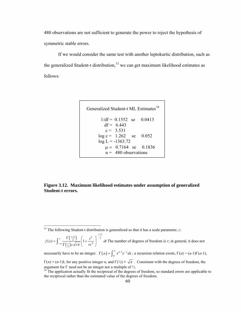
60

480 observations are not sufficient to generate the power to reject the hypothesis of

symmetric stable errors.

If we would consider the same test with another leptokurtic distribution, such as

the generalized Student-t distribution,33 we can get maximum likelihood estimates as

follows:

Generalized Student-t ML Estimates34

1/df = 0.1552 se 0.0413 df = 6.443

c = 3.531 log c = 1.262 se 0.052 log L = -1363.72 μ = 0.7164 se 0.1836

n = 480 observations

Figure 3.12. Maximum likelihood estimates under assumption of generalized Student-t errors.

33 The following Student-t distribution is generalized so that it has a scale parameter, c:

( )( )

11 2 22

22

( ) 1

rr

x

r

tf x dtrcc rπ

+−+

−∞

Γ ⎛ ⎞= +⎜ ⎟

Γ ⎝ ⎠∫ The number of degrees of freedom is r; in general, it does not

necessarily have to be an integer. ( ) 10

a xa x e dx∞ − −Γ = ∫ ; a recursion relation exists, Γ(a) = (a-1)Γ(a-1),

Γ(n) = (n-1)!, for any positive integer n, and Γ(½) = π . Consistent with the degrees of freedom, the argument for Γ need not be an integer nor a multiple of ½. 34 The application actually fit the reciprocal of the degrees of freedom, so standard errors are applicable to the reciprocal rather than the estimated value of the degrees of freedom.

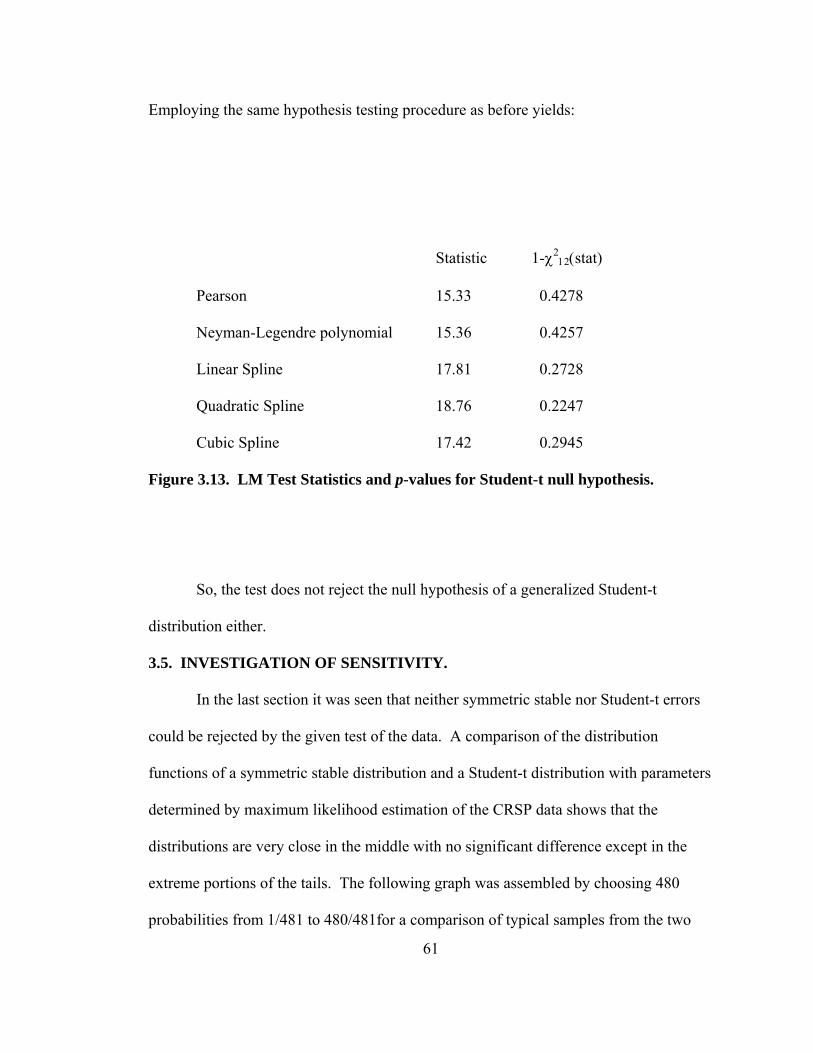
61

Employing the same hypothesis testing procedure as before yields:

Statistic 1-χ212(stat)

Pearson 15.33 0.4278

Neyman-Legendre polynomial 15.36 0.4257

Linear Spline 17.81 0.2728

Quadratic Spline 18.76 0.2247

Cubic Spline 17.42 0.2945

Figure 3.13. LM Test Statistics and p-values for Student-t null hypothesis.

So, the test does not reject the null hypothesis of a generalized Student-t

distribution either.

3.5. INVESTIGATION OF SENSITIVITY.

In the last section it was seen that neither symmetric stable nor Student-t errors

could be rejected by the given test of the data. A comparison of the distribution

functions of a symmetric stable distribution and a Student-t distribution with parameters

determined by maximum likelihood estimation of the CRSP data shows that the

distributions are very close in the middle with no significant difference except in the

extreme portions of the tails. The following graph was assembled by choosing 480

probabilities from 1/481 to 480/481for a comparison of typical samples from the two

62

distributions of the same sample size as the data. The ordinates were determined by

applying the respective inverse distribution functions to the vector of probabilities.

t(6.4434,3.5310) vs. ss(1.8824,2.7414)

-20

-15

-10

-5

0

5

10

15

20

0 0.2 0.4 0.6 0.8 1t

ss

Figure 3.14. Comparison of inverse distribution functions of Student-t and symmetrical stable error distributions at MLE.

An expanded view of the tail region (48 points) allows the slight differences between

the distributions to be discerned:

63

t(6.4434,3.5310) vs. ss(1.8824,2.7414)

0

2

4

6

8

10

12

14

16

18

20

0.9 0.92 0.94 0.96 0.98 1

tss

Figure 3.15. Comparison of upper tail of inverse distribution functions of Student-t and symmetrical stable error distributions at MLE.

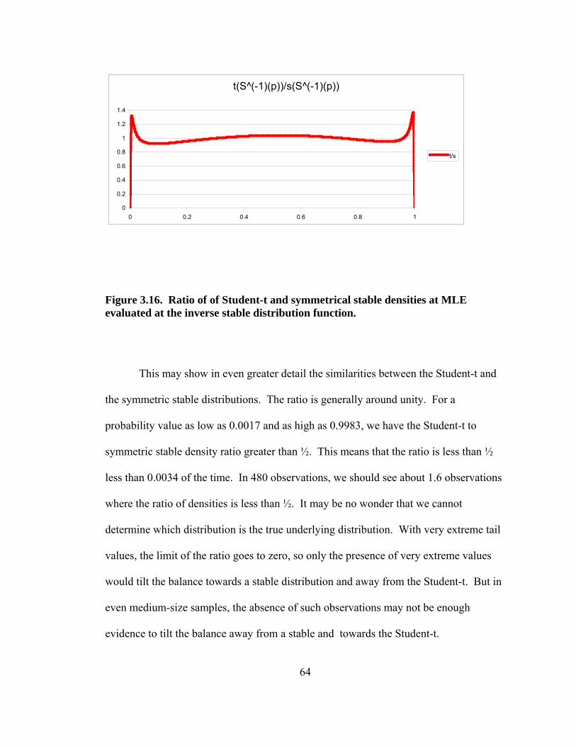
64

t(S^(-1)(p))/s(S^(-1)(p))

0

0.2

0.4

0.6

0.8

1

1.2

1.4

0 0.2 0.4 0.6 0.8 1

t/s

Figure 3.16. Ratio of of Student-t and symmetrical stable densities at MLE evaluated at the inverse stable distribution function.

This may show in even greater detail the similarities between the Student-t and

the symmetric stable distributions. The ratio is generally around unity. For a

probability value as low as 0.0017 and as high as 0.9983, we have the Student-t to

symmetric stable density ratio greater than ½. This means that the ratio is less than ½

less than 0.0034 of the time. In 480 observations, we should see about 1.6 observations

where the ratio of densities is less than ½. It may be no wonder that we cannot

determine which distribution is the true underlying distribution. With very extreme tail

values, the limit of the ratio goes to zero, so only the presence of very extreme values

would tilt the balance towards a stable distribution and away from the Student-t. But in

even medium-size samples, the absence of such observations may not be enough

evidence to tilt the balance away from a stable and towards the Student-t.

65

Next we see what happens if we actually know the underlying distribution.

What can we expect? This test uses a generated series of 480 observations from a

Student-t distribution with 6.4434 degrees of freedom, a scale factor 3.5310, with a

location parameter of 0.7164. Not surprisingly, at this number of observations, similar

tests to those previously employed do not allow summary rejection of a null hypothesis

of an underlying symmetric stable series. The maximum likelihood estimates of the

earlier symmetric stable fitting of the CRSP data is included below for comparison.

66

Series: Random Student-t Series: CRSP data

Random Seed 04579384 (hex)

Symmetric Stable ML Estimates Symmetric Stable ML Estimates

a = 1.7814 se 0.0781 a = 1.8450 se 0.0658 c = 2.7441 c = 2.7113

log c = 1.0094 se 0.0479 log c = 0.9974 se 0.0433 log L = -1384.4738 log L = -1364.7445

μ = 0.6325 se 0.1875 μ = 0.6729 se 0.1840 n = 480 observations n = 480 observations

Statistic 1-χ2

12(stat)

Pearson 11.84 0.6911 Neyman-Legendre polynomial 6.32 0.9738 Linear Spline 20.16 0.1657 Quadratic Spline 32.94 0.0048 Cubic Spline 42.41 0.0002

Figure 3.17. Tests of a null of symmetric stable distribution with an underlying Student-t distribution, sample size 480.

Prior to commenting on the above statistics, it may be instructive to view

another simulation:

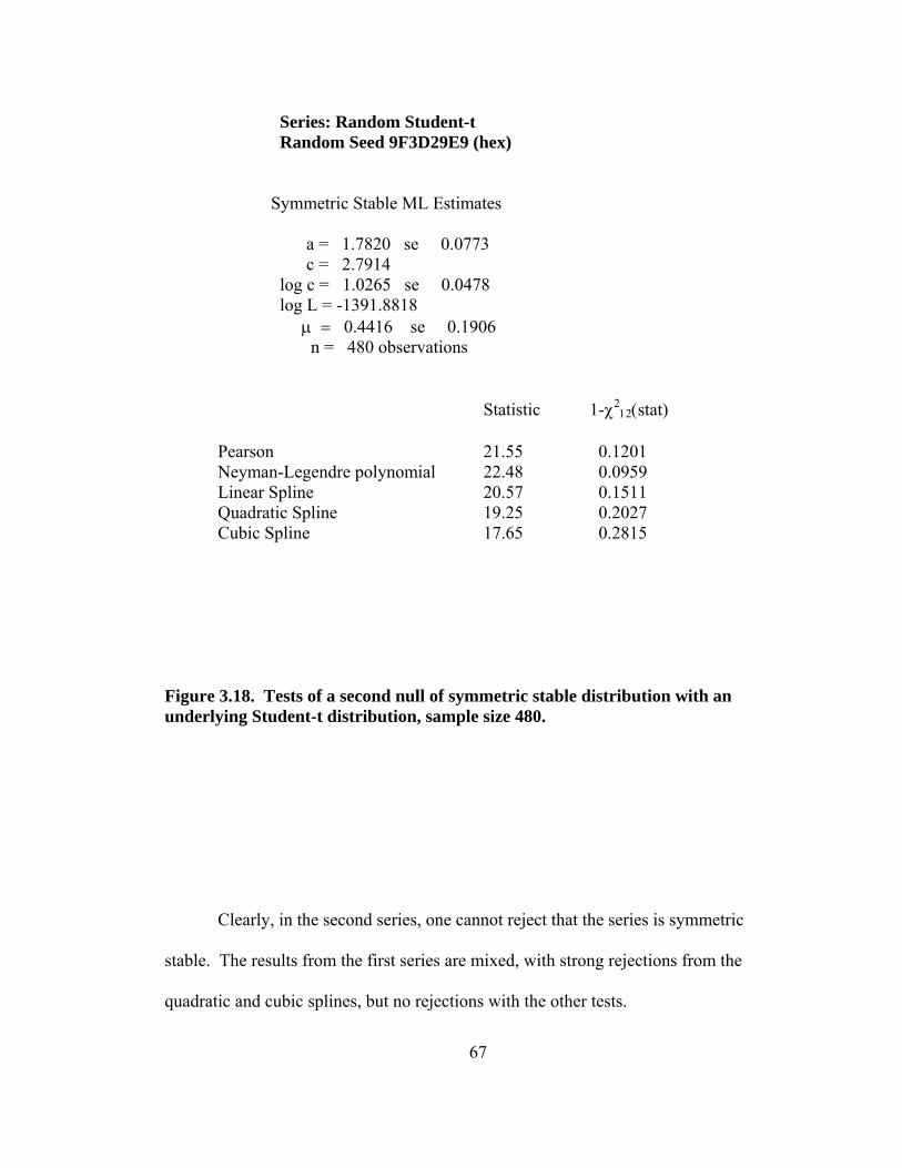
67

Series: Random Student-t Random Seed 9F3D29E9 (hex)

Symmetric Stable ML Estimates

a = 1.7820 se 0.0773 c = 2.7914

log c = 1.0265 se 0.0478 log L = -1391.8818

μ = 0.4416 se 0.1906 n = 480 observations

Statistic 1-χ212(stat)

Pearson 21.55 0.1201

Neyman-Legendre polynomial 22.48 0.0959 Linear Spline 20.57 0.1511 Quadratic Spline 19.25 0.2027 Cubic Spline 17.65 0.2815

Figure 3.18. Tests of a second null of symmetric stable distribution with an underlying Student-t distribution, sample size 480.

Clearly, in the second series, one cannot reject that the series is symmetric

stable. The results from the first series are mixed, with strong rejections from the

quadratic and cubic splines, but no rejections with the other tests.

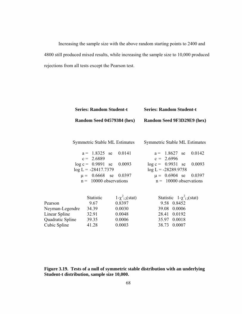
68

Increasing the sample size with the above random starting points to 2400 and

4800 still produced mixed results, while increasing the sample size to 10,000 produced

rejections from all tests except the Pearson test.

Series: Random Student-t Series: Random Student-t

Random Seed 04579384 (hex) Random Seed 9F3D29E9 (hex)

Symmetric Stable ML Estimates Symmetric Stable ML Estimates

a = 1.8325 se 0.0141 a = 1.8627 se 0.0142 c = 2.6889 c = 2.6996

log c = 0.9891 se 0.0093 log c = 0.9931 se 0.0093 log L = -28417.7379 log L = -28289.9758

μ = 0.6668 se 0.0397 μ = 0.6904 se 0.0397 n = 10000 observations n = 10000 observations

Statistic 1-χ212(stat) Statistic 1-χ2

12(stat)

Pearson 9.67 0.8397 9.58 0.8452 Neyman-Legendre 34.39 0.0030 39.08 0.0006 Linear Spline 32.91 0.0048 28.41 0.0192 Quadratic Spline 39.35 0.0006 35.97 0.0018 Cubic Spline 41.28 0.0003 38.73 0.0007

Figure 3.19. Tests of a null of symmetric stable distribution with an underlying Student-t distribution, sample size 10,000.

69

The bad news is that with limited data, densities that are similar over much of

their support cannot be distinguished from each other very easily. This does not allow

one to make very strong statements about the tail probabilities where the densities differ

considerably. Although this data set has only 480 monthly returns, 50 years of daily

returns would yield about 12,500 observations, so it is not unrealistic that one could

observe sample sizes of 10,000 or even larger. When daily data is used the returns

become less independent and less identically distributed since there is more apparent

volatility clustering, day-of-the-week effects in both mean and scale, holiday effects,

end-of-year effects, among other complications. However, the method shown here of

maximum likelihood estimation allows these extra considerations to be estimated

without biasing the results.

Some studies use tick-by-tick Foreign Exchange rate data. At that frequency,

transaction costs start to become a major consideration, so the returns are difficult to

analyze, but now more than ever samples might have 100,000 or even 1,000,000

observations. So 10,000 may in some senses still be a “small” sample.

70

CHAPTER 4

RESULTS OF OTHER GFTS

4.1 RESIDUAL TESTS.

Many goodness-of-fit tests implicitly rely on residuals being distributed

identically to the typically unknown error terms. Unless the model parameter terms are

known with certainty, most parameters must be estimated. During that estimation

parameters are chosen to fit the residuals as nearly as possible to the assumed error

distribution. The result is that residual tests will tend to be biased towards acceptance

of the null hypothesis.

The symmetric stable case presented before can serve as an illustration. The

first table below shows, in the left column, relative levels of significance when the

hypothesis tests take into consideration possible model improvement by considering

changes the model parameters as well as changes in the error distribution. The right

column shows levels of significance when the estimated model parameters are taken as

fixed and only changes in the error distribution are considered. The 90 tests are five

tests each (Pearson, Neyman, and the three Spline tests) using from 3 to 20 free

parameters to test the symmetric stable distribution.

71

Frequency of Tests by Level of Significance

Level of Significance Corrected Test Naïve Test

≤ 0.05 3 1 0.05-0.10 1 0 0.10-0.15 0 1 0.15-0.20 9 1 0.20-0.30 24 8 0.30-0.40 32 30 0.40-0.50 8 28 0.50-0.60 4 14 0.60-0.70 3 1 0.70-0.80 4 3 0.80-0.90 0 1 0.90-1.00 1 2

N/A 135 0

Figure 4.1. Comparison of results of 90 tests where the null hypothesis and the underlying distributions were both symmetric stable distributions.

35 A Pearson statistic that was negative was eliminated since no Complement of the Inverse Chi-Squared Distribution statistic is available. The procedure employed uses an estimate of the Fisher information matrix which is not guaranteed to be positive definite. Some test-statistics can be negative. The next section will elucidate this matter.

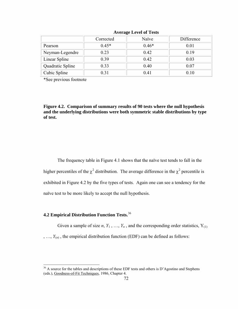
72

Average Level of Tests Corrected Naïve Difference Pearson 0.45* 0.46* 0.01 Neyman-Legendre 0.23 0.42 0.19 Linear Spline 0.39 0.42 0.03 Quadratic Spline 0.33 0.40 0.07 Cubic Spline 0.31 0.41 0.10 *See previous footnote

Figure 4.2. Comparison of summary results of 90 tests where the null hypothesis and the underlying distributions were both symmetric stable distributions by type of test.

The frequency table in Figure 4.1 shows that the naïve test tends to fall in the

higher percentiles of the χ2 distribution. The average difference in the χ2 percentile is

exhibited in Figure 4.2 by the five types of tests. Again one can see a tendency for the

naïve test to be more likely to accept the null hypothesis.

4.2 Empirical Distribution Function Tests.36

Given a sample of size n, Y1 , …, Yn , and the corresponding order statistics, Y(1)

, …, Y(n) , the empirical distribution function (EDF) can be defined as follows:

36 A source for the tables and descriptions of these EDF tests and others is D’Agostino and Stephens (eds.), Goodness-of-Fit Techniques, 1986, Chapter 4.

73

(1)

( ) ( 1)

( )

0

( )

1

ii in

n

y Y

EDF y Y y Y

Y y+

⎧ −∞ < <⎪

= < <⎨⎪ < < ∞⎩

, i = 1 , 2 , …, n - 1

Many EDF tests have been around for half a century or more. It seems natural

to compare the previous results to these tests. These tests have an assumption of a

completely specified distribution. When the parameters have been determined by some

optimization method such as maximum likelihood, as discussed in the previous section,

inferences are less accurate.

The most common empirical distribution goodness-of-fit test is based on the

Kolmogorov-Smirnoff (KS) statistic. It seeks to look at the largest single difference

between the assumed distribution, F(y) and the EDF, so it can be described as:

( ) ( )supy

KS EDF y F y= −

Two other common EDF tests are the Cramér-von Mises (CvM) statistic and an

Anderson-Darling (AD) modification of CvM. The CvM statistic is the integrated

squared difference between the EDF and the assumed distribution. The AD

modification is based on the premise that one should examine the difference in the tails

of the distributions more closely than the center of the distribution, which is

accomplished by dividing by a function that takes its maximum value at the median of

the distribution.

74

( ) ( )

( ) ( )( ) ( )

2*

2*

* *1

CvM n EDF y F y dy

EDF y F yAD n dy

F y F y

∞

−∞

∞

−∞

⎡ ⎤= −⎣ ⎦

⎡ ⎤−⎣ ⎦=⎡ ⎤−⎣ ⎦

∫

∫

In the expressions above ( ) ( )*F y U F y= ⎡ ⎤⎣ ⎦ where U(y) is the distribution

function for a uniform random variable on the unit interval. By using this

transformation and sample size adjustment factors for KS and CvM, standard tables of

critical values can be employed.

The results for the CRSP data follow:

Kolmogorov-Smirnov Stable Student Gaussian Base Statistic 0.039 0.039 0.053

Modified 0.855 0.870 1.167 Significance >0.250 >0.250 0.129

Cramér-von Mises Base Statistic 0.099 0.097 0.305

Modified 0.098 0.096 0.305 Significance >0.250 >0.250 0.129

Anderson-Darling Statistic 0.793 0.813 2.046

Significance >0.250 >0.250 0.083

Figure 4.3 Empirical Distribution Functions of CRSP data.

75

At conventional significance levels none of these tests would reject any of the

posited distributions; however, the Gaussian tests appear to be in the weaker range of

statistics indicating non-rejection.

76

CHAPTER 5

IMPROVEMENTS IN RESULTS DUE TO NUMERICAL QUADRATURE OF FISHER INFORMATION MATRIX

5.1 DERIVATION OF FISHER INFORMATION MATRIX

The application of Lagrange multiplier tests in this research has relied on using

consistent estimators for the Fisher information matrix. Especially with distributions

such as the symmetric stable with no closed form for even its corresponding density

function, numerical estimation of many of the components of the test statistic is

necessary. When the Fisher information matrix is unavailable, consistent estimators

such as the negative of empirical Hessian or the outer-product-of-the-gradient (OPG)

estimator become likely candidates for substitution. When computing the Fisher

information matrix the only stochastic aspect is the vector of maximum likelihood

estimates. The use of the empirical Hessian or the OPG estimators inherently imparts

more noise to the tests. And, per Davidson and McKinnon, the OPG estimator “often

seems to be particularly poor.”37

In the example above, use was made of a hybrid matrix, with some of its entries

actually being entries from the Fisher information matrix, some being entries from the

negative of the empirical Hessian, and some being entries from the OPG estimator.

37 Davidson and MacKinnon, Estimation and Inference in Econometrics, p. 266.

77

Since a consistent matrix estimator consistently estimates each entry in the matrix, such

a hybrid must also be a consistent matrix estimator.

Let’s examine the makeup of typical hybrid estimator.

( ) ( ) ( )

( ) ( ) ( )

2

1 1

21

0 ˆ1 10

ln ln ln

;ln ln ln

n ni i i

k k k ji i

n ni i i

ij k j ji i

L y L y L y

L y L y L yn dy

θ θα

θ θ θ α

α θ α α

′= =

′= = ==

⎡ ⎤∂ ∂ ∂−⎢ ⎥

∂ ∂ ∂⎢ ⎥⎢ ⎥⎡ ⎤∂ ∂ ∂⎢ ⎥−⎢ ⎥⎢ ⎥∂ ∂ ∂⎢ ⎥⎣ ⎦⎣ ⎦

∑ ∑

∑ ∑∫

, 1, 2, , ; , 1, ,j j m k k K′ ′= =K K

The upper left portion of the matrix measures the curvature of the log likelihood

with respect to the model parameters. For the stable and Student-t tests, a numerical

estimate of empirical Hessian was used; for the Gaussian test, the actual Fisher

information matrix was used.

The lower right portion of the matrix shows the curvature with respect to the

perturbation parameters in the density of the alternate hypothesis. Given the basis

functions chosen, exact analytical calculation of the Fisher information matrix was

straightforward.

The off diagonal elements are estimated via OPG estimation, which perhaps is

the noisiest of the three methods.

In addition to the noise, another inconvenient feature of this hybrid matrix is that

it is not guaranteed to be positive definite. Even though the test statistics are

asymptotically chi-squared, they can be negative in finite samples.

78

After the employment of these tests, we have determined that we may be able

always to determine the empirical Hessian and perhaps always to numerically estimate

the Fisher information matrix which has led to more accurate finite sample results.

Following are the details of the recent calculations:

Given the nested hypotheses test,

H0: yi ~ F(y;θ) vs. H1: yi ~ G[F(y;θ)],

with the density for the alternative hypothesis being

g[F(y;θ)] f(y;θ), where ( ) ( )1

1m

j jj

g z zα φ=

= + ∑ ,

the likelihood and log likelihood functions are:

( ) ( )1

( , ; ) ; ; ;n

i ii

L y g F f yα θ ε θ α θ=

⎡ ⎤= ⎣ ⎦∏ and

( ) ( )1 1

log ( , ; ) log ; ; log ;n n

i ii i

L y g F y f yα θ θ α θ= =

⎡ ⎤= +⎣ ⎦∑ ∑

The first derivatives of the log likelihood are:

( )( ) ( )

( )( )( )( )

1 1 1

1

1

log ( , ; ) log 1 ; log ;

;

1 ;

n m n

j j i ij j i j i

nj i

mi

j j ij

L y F y f y

F y

F y

α θ α φ θ θα α

φ θ

α φ θ

= = =

=

=

⎛ ⎞⎛ ⎞∂ ∂⎜ ⎟= + +⎜ ⎟⎜ ⎟⎜ ⎟∂ ∂ ⎝ ⎠⎝ ⎠

=+

∑ ∑ ∑

∑∑

and

( )( ) ( )1 1 1

log ( , ; ) log 1 ; log ;n m n

j j i ik k i j i

L y F y f yα θ α φ θ θθ θ = = =

⎛ ⎞⎛ ⎞∂ ∂⎜ ⎟= + + =⎜ ⎟⎜ ⎟⎜ ⎟∂ ∂ ⎝ ⎠⎝ ⎠∑ ∑ ∑

79

( )( ) ( )

( )( )

( )

( )1

1 1

1

; ; ;

;1 ;

m

j j i i in nkj k

mii i

j j ij

F fF y y y

f yF y

α φ θ θ θθ θθ

α φ θ

=

= =

=

∂ ∂′∂ ∂

++

∑∑ ∑

∑

Evaluation at the maximum log likelihood of the restricted model, θθα ˆ,0 == , yields:

( )( )0 1ˆ

log ( , ; ) ˆ;n

j ij i

L y F yαθ θ

α θ φ θα = =

=

∂=

∂ ∑ and ( )

( )0 1ˆ

ˆ;log ( , ; )

ˆ;

ink

k i i

f yL y

f yαθ θ

θθα θ

θ θ= ==

∂∂∂

=∂ ∑

The second derivatives of the log likelihood are:

( )( )( )( )

( )( ) ( )( )

( )( )

2

21 1

1 1

; ; ;log ( , ; )

1 ; 1 ;

n nj i j i j i

m mj j j i ih h i h h i

h h

F y F y F yL y

F y F y

φ θ φ θ φ θα θα α α

α φ θ α φ θ

′

′ ′ = =

= =

⎛ ⎞⎜ ⎟ −∂ ∂ ⎜ ⎟= =⎜ ⎟∂ ∂ ∂ ⎡ ⎤+⎜ ⎟ +⎢ ⎥⎝ ⎠ ⎣ ⎦

∑ ∑∑ ∑

,

( )( ) ( )

( )( )

( )

( )2

1

1 1

1

; ; ;log ( , ; )

;1 ;

m

j j i i in nkj k

mk k k ii i

j j ij

F fF y y yL y

f yF y

α φ θ θ θθ θα θθ θ θ θ

α φ θ

=

′ ′ = =

=

⎛ ⎞∂ ∂′⎜ ⎟∂ ∂∂ ∂ ⎜ ⎟= + =⎜ ⎟∂ ∂ ∂+⎜ ⎟⎜ ⎟

⎝ ⎠

∑∑ ∑

∑

( )( ) ( )( ) ( ) ( ) ( )( ) ( )

( )( )

2

1 12

1

1

1 ; ; ; ; ; ;

1 ;

m m

j j i j j i i i j i in j j k k k k

mi

j j ij

F F FF y F y y y F y y

F y

α φ θ α φ θ θ θ φ θ θθ θ θ θ

α φ θ

′ ′= =

=

=

⎡ ⎤ ⎡ ⎤⎛ ⎞∂ ∂ ∂′′ ′+ +⎢ ⎥ ⎢ ⎥⎜ ⎟∂ ∂ ∂ ∂⎢ ⎥ ⎢ ⎥⎝ ⎠⎣ ⎦ ⎣ ⎦

⎡ ⎤+⎢ ⎥

⎢ ⎥⎣ ⎦

∑ ∑∑

∑

( )( ) ( ) ( )( ) ( )

( )( )

1 12

1

1

; ; ; ;

1 ;

m m

j j i i j j i in k kj j

mi

j j ij

F FF y y F y y

F y

α φ θ θ α φ θ θθ θ

α φ θ

′= =

=

=

⎡ ⎤ ⎡ ⎤∂ ∂′ ′⎢ ⎥ ⎢ ⎥∂ ∂⎢ ⎥ ⎢ ⎥⎣ ⎦ ⎣ ⎦−⎡ ⎤

+⎢ ⎥⎢ ⎥⎣ ⎦

∑ ∑∑

∑

( ) ( ) ( ) ( )

( )

2

21

; ; ; ;

;

i i i ink k k k

i i

f f ff y y y y

f y

θ θ θ θθ θ θ θ

θ′ ′

= ⎡ ⎤⎣ ⎦

∂ ∂ ∂−∂ ∂ ∂ ∂

+∑

80

and, first differentiating with respect to αj, and then differentiating with respect to θk

(for ease of calculation),

( )( )( )( )

2

1

1

;log ( , ; )

1 ;

nj i

mk j k i

j j ij

F yL y

F y

φ θα θθ α θ

α φ θ=

=

⎛ ⎞⎜ ⎟

∂ ∂ ⎜ ⎟= =⎜ ⎟∂ ∂ ∂+⎜ ⎟⎜ ⎟

⎝ ⎠

∑∑

( )( ) ( )( ) ( ) ( )( ) ( )( ) ( )

( )( )

1 12

1

1

1 ; ; ; ; ; ;

1 ;

m m

j j i j i i j i j j i in k kj j

mi

j j ij

F FF y F y y F y F y y

F y

α φ θ φ θ θ φ θ α φ θ θθ γ

α φ θ

= =

=

=

⎡ ⎤ ∂ ∂′ ′+ −⎢ ⎥∂ ∂⎢ ⎥⎣ ⎦

⎡ ⎤+⎢ ⎥

⎢ ⎥⎣ ⎦

∑ ∑∑

∑

These expressions simplify greatly at the maximized log likelihood of the restricted

model, θθα ˆ,0 == :

( )( ) ( )( )2

0 1ˆ

log ( , ; ) ˆ ˆ; ;n

j i j ij j i

L y F y F yαθ θ

α θ φ θ φ θα α ′

=′ ==

∂= −

∂ ∂ ∑

( ) ( ) ( ) ( )( )

2

2

20 1ˆ

ˆ ˆ ˆ ˆ; ; ; ;log ( , ; )

ˆ;

i i i ink k k k

k k ii

f f ff y y y yL y

f yαθ θ

θ θ θ θθ θ θ θα θ

θ θ θ

′ ′

=′ ==

∂ ∂ ∂−

∂ ∂ ∂ ∂∂=

∂ ∂ ⎡ ⎤⎣ ⎦

∑

( )( ) ( )2

0 1ˆ

log ( , ; ) ˆ ˆ; ;n

j i ik j ki

L y FF y yαθ θ

α θ φ θ θθ α θ= =

=

∂ ∂′=∂ ∂ ∂∑

It is possible to perform the expectation integration for some distribution

functions to get the Fisher information matrix directly. But, in any case it is always

reasonable to get an empirical Hessian, by substituting residuals from the restricted

estimate for the unknown error terms. All that is necessary to determine the mixed

second derivatives is to (1) differentiate the chosen basis functions, (2) numerically

evaluate the chosen distribution, using maximum likelihood estimates for parameters, at

81

each residual, and (3) numerically differentiate the distribution function at each

residual.

To get the full Fisher information matrix directly, we need to solve:

( )( ) ( )( ) ( ); ; ;j jn F y F y f y dyφ θ φ θ θ∞

′−∞∫ for the lower right entries,

( ) ( )

( )

; ;

;k k

f fy yn dy

f y

θ θθ θ

θ∞ ′−∞

∂ ∂∂ ∂

⎡ ⎤⎣ ⎦∫ for the upper left entries, and

( )( ) ( ) ( ); ; ;jk

Fn F y y f y dyφ θ θ θθ

∞

−∞

∂′−∂∫ for the off diagonal entries.

Numerical quadrature can be employed with a transformation to a finite interval.

Another form for the last integral is ( )( ) ( );;j

k

f yn F y dy

θφ θ

θ∞

−∞

∂∂∫ , which is

derived from the expected value of the OPG. These two expressions can be shown to

be equal by the method of integration by parts:

( )( ) ( );;j

k

f yF y dy

θφ θ

θ∞

−∞

∂=

∂∫

( )( ) ( ) ( )( ) ( ) ( ); ;; ; ;

y

j jk ky

F y F yF y F y f y dy

θ θφ θ φ θ θ

θ θ

=∞∞

−∞=−∞

∂ ∂⎤ ′− =⎥∂ ∂⎦∫

( )( ) ( ) ( )( ) ( )

( )( ) ( ) ( )

; ;lim ; lim ;

;; ;

j jy yk k

jk

F y F yF y F y

F yF y f y dy

θ θφ θ φ θ

θ θ

θφ θ θ

θ

→∞ →−∞

∞

−∞

∂ ∂⎡ ⎤ ⎡ ⎤−⎢ ⎥ ⎢ ⎥∂ ∂⎣ ⎦ ⎣ ⎦

∂′− =∂∫

82

( ) ( ) ( ) ( ) ( )( ) ( ) ( )

( )( ) ( ) ( )

0

;1 0 0 0 ; ;

;; ;

j j jk

jk

F yF y f y dy

F yF y f y dy

θφ φ φ θ θ

θ

θφ θ θ

θ

∞

−∞=

∞

−∞

∂′− − =∂

∂′−∂

∫

∫

144424443, since

( ) ( )lim ; 1 lim ; 0y y

F y and F yθ θ→∞ →−∞

= =⎡ ⎤ ⎡ ⎤⎣ ⎦ ⎣ ⎦ , which are both constants, so the limit of

the derivative must be zero.

5.2 NUMERICAL TWO-SIDED DIFFERENTIATION38

Attempting direct integration of the elements of the Fisher information matrix

becomes quite a numerical challenge to produce estimates that are accurate enough for

matrix inversion and to produce accurate Lagrange multiplier statistics. A method called

Richardson extrapolation, of which a Romberg integration technique is a special case, is

employed to obtain more accurate evaluations of derivatives and integrals than is

possible with the same effort by using less complicated but more direct numerical

methods.

It is desirable to use two-sided numerical differences to approximate derivatives

when possible because, as will be shown, it is more accurate than its one-sided

counterpart. This is because second order terms are automatically eliminated with the

two-sided approach.

Unfortunately, in some situations, such as determining the derivatives of stable

distributions when the shape parameter is near 2, one can only perform one-sided

38 Significant inspiration for some of the methodologies described in the next several sections was derived from Fundamentals of Numerical Analysis, Stephen G. Kellison, Richard D. Irwin, Inc., 1975 and A First Course in Numerical Analysis, Anthony Ralston and Philip Rabinowitz, Dover Publications, Inc., 1978.

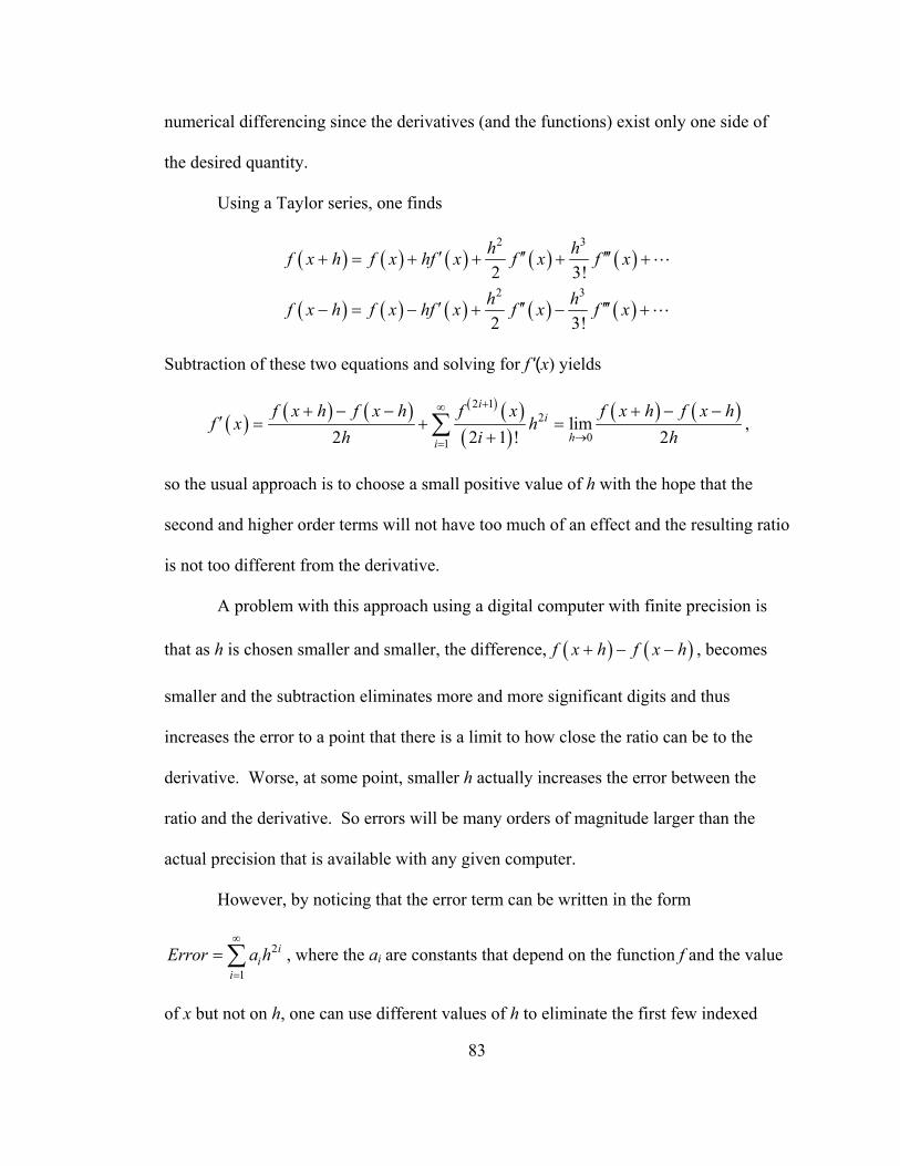
83

numerical differencing since the derivatives (and the functions) exist only one side of

the desired quantity.

Using a Taylor series, one finds

( ) ( ) ( ) ( ) ( )

( ) ( ) ( ) ( ) ( )

2 3

2 32 3!

2 3!

h hf x h f x hf x f x f x

h hf x h f x hf x f x f x

′ ′′ ′′′+ = + + + +

′ ′′ ′′′− = − + − +

L

L

Subtraction of these two equations and solving for f '(x) yields

( ) ( ) ( ) ( ) ( )( )

( ) ( )2 12

01lim

2 2 1 ! 2

ii

hi

f x h f x h f x f x h f x hf x h

h i h

+∞

→=

+ − − + − −′ = + =

+∑ ,

so the usual approach is to choose a small positive value of h with the hope that the

second and higher order terms will not have too much of an effect and the resulting ratio

is not too different from the derivative.

A problem with this approach using a digital computer with finite precision is

that as h is chosen smaller and smaller, the difference, ( ) ( )f x h f x h+ − − , becomes

smaller and the subtraction eliminates more and more significant digits and thus

increases the error to a point that there is a limit to how close the ratio can be to the

derivative. Worse, at some point, smaller h actually increases the error between the

ratio and the derivative. So errors will be many orders of magnitude larger than the

actual precision that is available with any given computer.

However, by noticing that the error term can be written in the form

2

1

ii

iError a h

∞

=

= ∑ , where the ai are constants that depend on the function f and the value

of x but not on h, one can use different values of h to eliminate the first few indexed

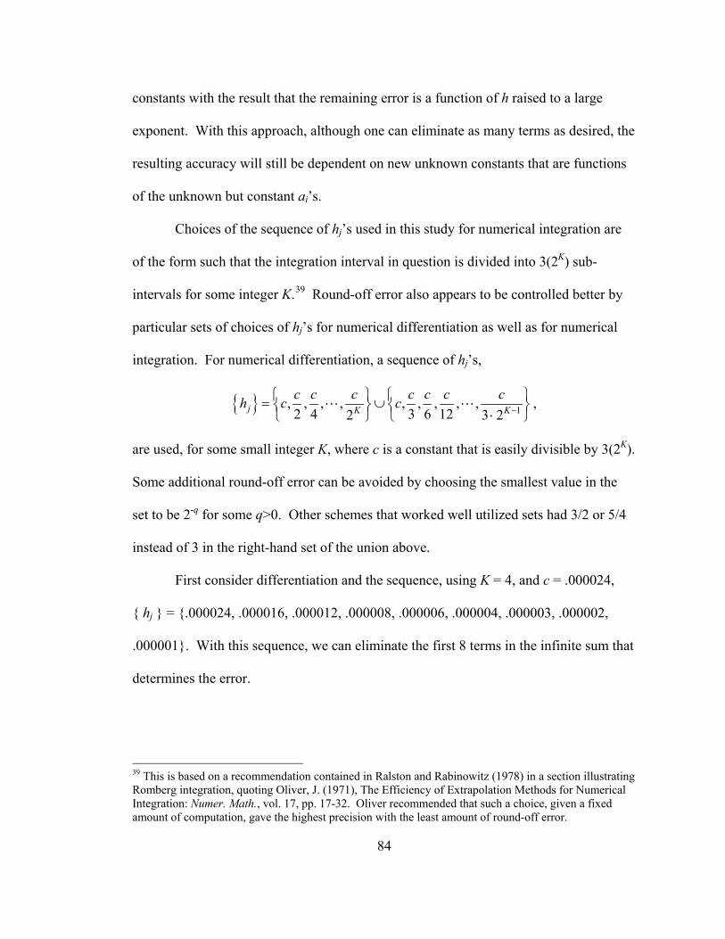
84

constants with the result that the remaining error is a function of h raised to a large

exponent. With this approach, although one can eliminate as many terms as desired, the

resulting accuracy will still be dependent on new unknown constants that are functions

of the unknown but constant ai’s.

Choices of the sequence of hj’s used in this study for numerical integration are

of the form such that the integration interval in question is divided into 3(2K) sub-

intervals for some integer K.39 Round-off error also appears to be controlled better by

particular sets of choices of hj’s for numerical differentiation as well as for numerical

integration. For numerical differentiation, a sequence of hj’s,

{ } 1, , , , , , , , ,2 4 3 6 122 3 2j K Kc c c c c c ch c c −

⎧ ⎫ ⎧ ⎫= ∪⎨ ⎬ ⎨ ⎬⋅⎩ ⎭ ⎩ ⎭

L L ,

are used, for some small integer K, where c is a constant that is easily divisible by 3(2K).

Some additional round-off error can be avoided by choosing the smallest value in the

set to be 2-q for some q>0. Other schemes that worked well utilized sets had 3/2 or 5/4

instead of 3 in the right-hand set of the union above.

First consider differentiation and the sequence, using K = 4, and c = .000024,

{ hj } = {.000024, .000016, .000012, .000008, .000006, .000004, .000003, .000002,

.000001}. With this sequence, we can eliminate the first 8 terms in the infinite sum that

determines the error.

39 This is based on a recommendation contained in Ralston and Rabinowitz (1978) in a section illustrating Romberg integration, quoting Oliver, J. (1971), The Efficiency of Extrapolation Methods for Numerical Integration: Numer. Math., vol. 17, pp. 17-32. Oliver recommended that such a choice, given a fixed amount of computation, gave the highest precision with the least amount of round-off error.

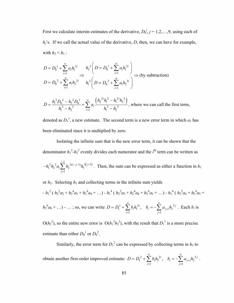
85

First we calculate interim estimates of the derivative, D0j, j = 1,2,…,9, using each of

hj’s. If we call the actual value of the derivative, D, then, we can have for example,

with h2 < h1 :

1 20 1

1

2 20 2

1

ii

i

ii

i

D D a h

D D a h

∞

=∞

=

= +

= +

∑

∑⇒

2 1 22 0 1

1

2 2 21 0 2

1

ii

i

ii

i

h D D a h

h D D a h

∞

=

∞

=

⎛ ⎞= +⎜ ⎟

⎝ ⎠⎛ ⎞

= +⎜ ⎟⎝ ⎠

∑

∑ ⇒ (by subtraction)

( )2 2 2 22 2 2 1 2 1 1 21 0 2 02 2 2 2

11 2 1 2

i i

ii

h h h hh D h DD ah h h h

∞

=

−−= +

− −∑ , where we can call the first term,

denoted as D11, a new estimate. The second term is a new error term in which a1 has

been eliminated since it is multiplied by zero.

Isolating the infinite sum that is the new error term, it can be shown that the

denominator h12-h2

2 evenly divides each numerator and the ith term can be written as

( )1

2 12 2 2( 1)1 2 2 1

1

iji j

ij

h h a h h−

−− −

=

− ∑ . Then, the sum can be expressed as either a function in h1

or h2. Selecting h1 and collecting terms in the infinite sum yields

- h12 ( h2

2a2 + h24a3 + h2

6a4 + …) - h14 ( h2

2a3 + h24a4 + h2

6a5 + …) - h16 ( h2

2a4 + h24a5 +

h26a6 + …) - … ; so, we can write 1 2 2

1 1 21 1

,i ji i j i

i jD D b h b a h

∞ ∞

+= =

= + = −∑ ∑ . Each bi is

O(h22), so the entire new error is O(h1

2h22), with the result that D1

1 is a more precise

estimate than either D01 or D0

2.

Similarly, the error term for D12 can be expressed by collecting terms in h3 to

obtain another first-order improved estimate: 2 2 21 3 2

1 1,i j

i i j ii j

D D b h b a h∞ ∞

+= =

= + = −∑ ∑ .

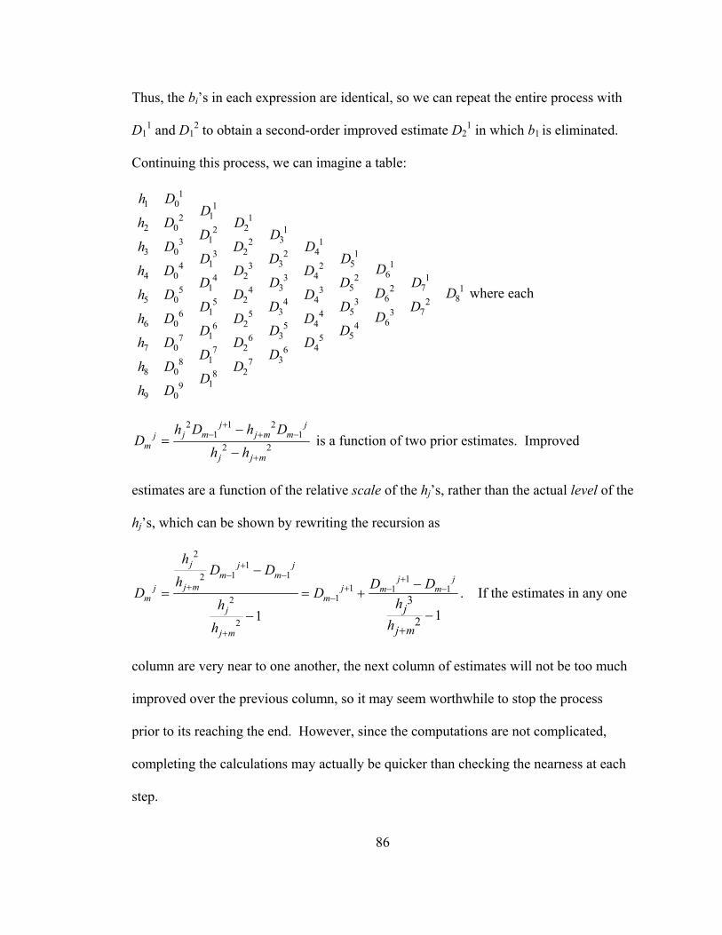
86

Thus, the bi’s in each expression are identical, so we can repeat the entire process with

D11 and D1

2 to obtain a second-order improved estimate D21 in which b1 is eliminated.

Continuing this process, we can imagine a table:

11 0 1

12 12 0 2 12

313 2 13 0 2 42 13

3 51 14 3 264 0 2 43 2 14

3 5 71 2 15 4 36 85 0 2 44 3 25

3 5 71 36 5 466 0 2 45 46

3 517 6 57 0 2 467

318 78 0 28

199 0

h DD

h D DDD

h D D DD DD

Dh D D DD D DD

D Dh D D DD D DD

Dh D D DD DD

h D D DDD

h D DD

h D

where each

2 1 21 1

2 2

j jj m j m mj

mj j m

h D h DD

h h

+− + −

+

−=

− is a function of two prior estimates. Improved

estimates are a function of the relative scale of the hj’s, rather than the actual level of the

hj’s, which can be shown by rewriting the recursion as

21

1 12 11 1 1

12

2

3

2 11

j j jm m j j

j mj j m mm m

j

j m

j

j m

hD D

h D DD Dh

h

hh

+− − +

+ + − −−

+ +

−−

= = +

−−

. If the estimates in any one

column are very near to one another, the next column of estimates will not be too much

improved over the previous column, so it may seem worthwhile to stop the process

prior to its reaching the end. However, since the computations are not complicated,

completing the calculations may actually be quicker than checking the nearness at each

step.

87

Additionally, with a consistent, repetitive choice of hj’s, one can save time by

solving the recursion directly in terms of the original estimates. After calculating the

original estimates, we can use the following linear combination. Approximate values

for K = 4, and c = .000024, shown to 4 significant digits, are:

1.693 D09 - 1.010 D0

8 + 0.3983 D07 – 0.08464 D0

6 + 0.003603 D05 – 0.0002004 D0

4 +

0.000001353 D03 – 0.00000001909 D0

2 + 0.00000000001226 D01

The above is shown to illustrate the relative size of the impact of the various

estimates. Of course, using only 4 significant digits would defeat the original purpose

of reducing error in the approximation.

The exact formula, using the original estimates, is:

* 1 2 3 40 0 0 0

5 6 7 80 0 0 0

90

1 27 32 2781587756250 1414538125 23648625 134750

32768 2592 536870912 8847369095625 30625 1347971625 875875144955146248561678125

D D D D D

D D D D

D

≈ − + −

+ − + −

+

Since many two-sided differentiations are required in some simulations,

considerable computational efficiency can be gained by calculating the end coefficients

a single time initially. This effectively reduces the calculations described over the

previous five pages to a GAUSS “proc” with roughly 15 lines of code in its body.

Often a relatively large value of the constant c allows for smaller absolute errors.

This is despite the fact that each of the initial estimates with the larger values of c

contains (absolutely) more error than it would with smaller values of c. Also, some

values using initial estimates may have small error unpredictably, based on the

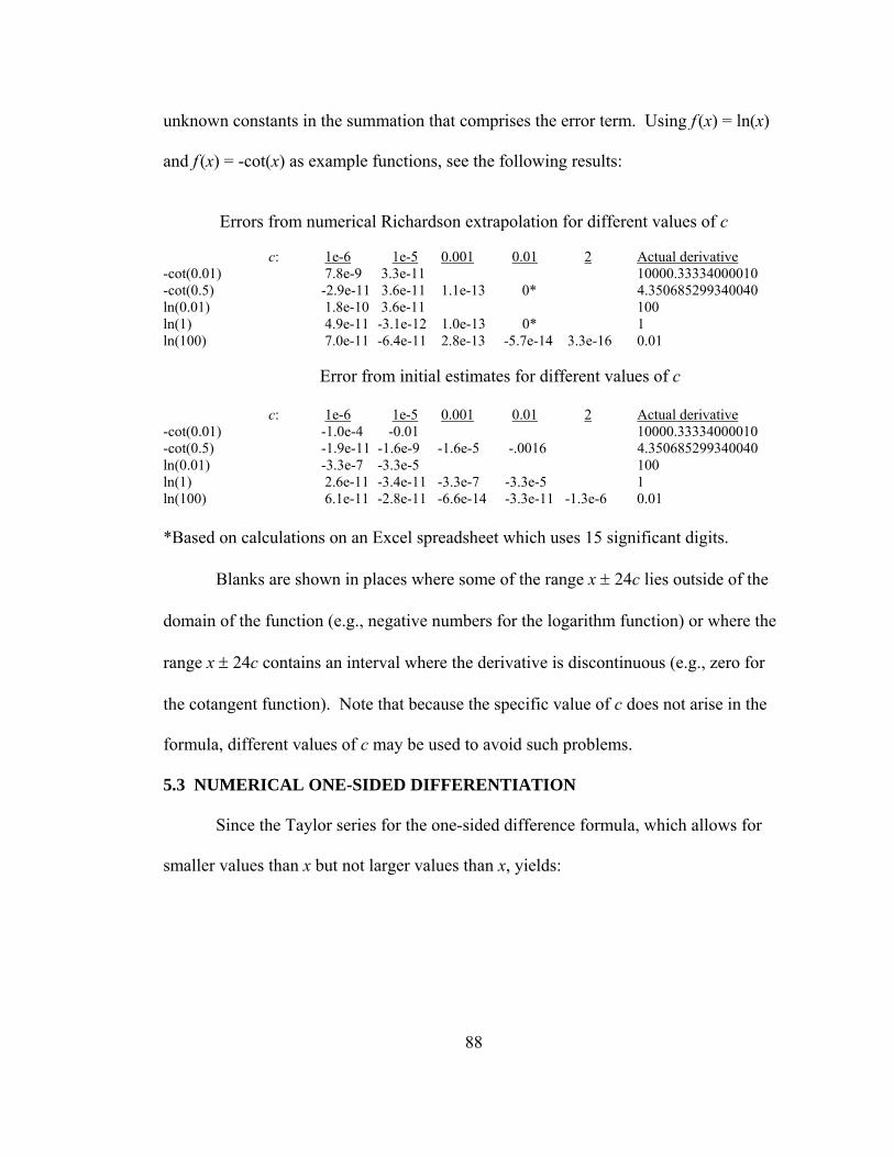
88

unknown constants in the summation that comprises the error term. Using f (x) = ln(x)

and f (x) = -cot(x) as example functions, see the following results:

Errors from numerical Richardson extrapolation for different values of c

c: 1e-6 1e-5 0.001 0.01 2 Actual derivative -cot(0.01) 7.8e-9 3.3e-11 10000.33334000010 -cot(0.5) -2.9e-11 3.6e-11 1.1e-13 0* 4.350685299340040 ln(0.01) 1.8e-10 3.6e-11 100 ln(1) 4.9e-11 -3.1e-12 1.0e-13 0* 1 ln(100) 7.0e-11 -6.4e-11 2.8e-13 -5.7e-14 3.3e-16 0.01

Error from initial estimates for different values of c

c: 1e-6 1e-5 0.001 0.01 2 Actual derivative -cot(0.01) -1.0e-4 -0.01 10000.33334000010 -cot(0.5) -1.9e-11 -1.6e-9 -1.6e-5 -.0016 4.350685299340040 ln(0.01) -3.3e-7 -3.3e-5 100 ln(1) 2.6e-11 -3.4e-11 -3.3e-7 -3.3e-5 1 ln(100) 6.1e-11 -2.8e-11 -6.6e-14 -3.3e-11 -1.3e-6 0.01 *Based on calculations on an Excel spreadsheet which uses 15 significant digits.

Blanks are shown in places where some of the range x ± 24c lies outside of the

domain of the function (e.g., negative numbers for the logarithm function) or where the

range x ± 24c contains an interval where the derivative is discontinuous (e.g., zero for

the cotangent function). Note that because the specific value of c does not arise in the

formula, different values of c may be used to avoid such problems.

5.3 NUMERICAL ONE-SIDED DIFFERENTIATION

Since the Taylor series for the one-sided difference formula, which allows for

smaller values than x but not larger values than x, yields:

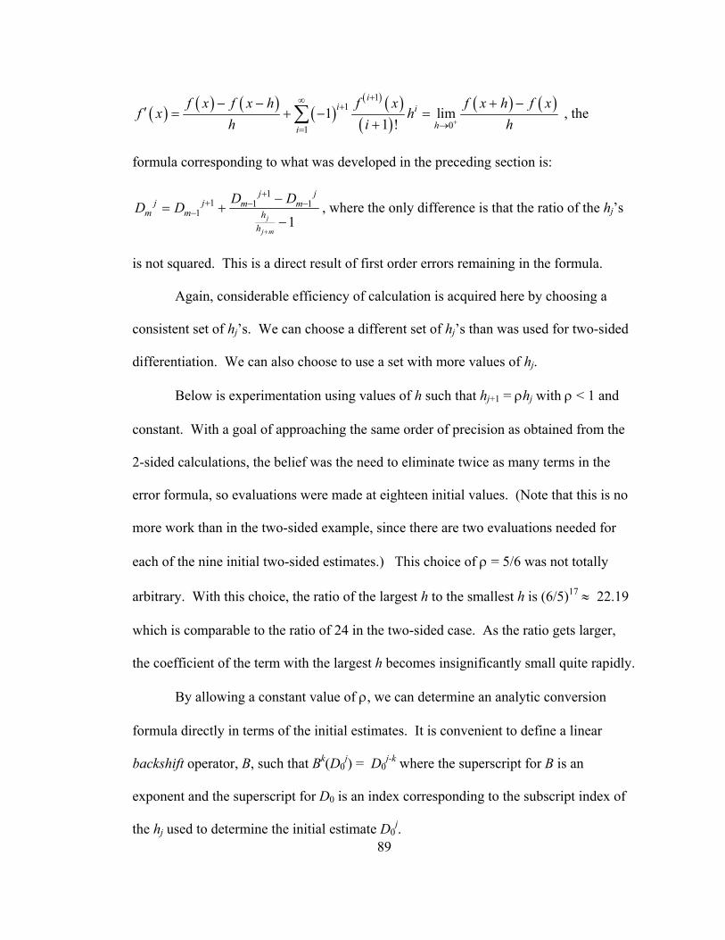
89

( ) ( ) ( ) ( )( ) ( )

( )( ) ( )1

1

011 lim

1 !

ii i

hi

f x f x h f x f x h f xf x h

h i h+

+∞+

→=

− − + −′ = + − =

+∑ , the

formula corresponding to what was developed in the preceding section is:

11 1 1

11j

j m

j jj j m m

m m hh

D DD D+

++ − −

−−

= +−

, where the only difference is that the ratio of the hj’s

is not squared. This is a direct result of first order errors remaining in the formula.

Again, considerable efficiency of calculation is acquired here by choosing a

consistent set of hj’s. We can choose a different set of hj’s than was used for two-sided

differentiation. We can also choose to use a set with more values of hj.

Below is experimentation using values of h such that hj+1 = ρhj with ρ < 1 and

constant. With a goal of approaching the same order of precision as obtained from the

2-sided calculations, the belief was the need to eliminate twice as many terms in the

error formula, so evaluations were made at eighteen initial values. (Note that this is no

more work than in the two-sided example, since there are two evaluations needed for

each of the nine initial two-sided estimates.) This choice of ρ = 5/6 was not totally

arbitrary. With this choice, the ratio of the largest h to the smallest h is (6/5)17 ≈ 22.19

which is comparable to the ratio of 24 in the two-sided case. As the ratio gets larger,

the coefficient of the term with the largest h becomes insignificantly small quite rapidly.

By allowing a constant value of ρ, we can determine an analytic conversion

formula directly in terms of the initial estimates. It is convenient to define a linear

backshift operator, B, such that Bk(D0j) = D0

j-k where the superscript for B is an

exponent and the superscript for D0 is an index corresponding to the subscript index of

the hj used to determine the initial estimate D0j.

90

With these definitions, ( )( )

( )180

17

156

56

117

1D

BD

jj

j

⎟⎟⎟

⎠

⎞

⎜⎜⎜

⎝

⎛

−

−= ∏

=

. This formula can be determined

by directly calculating the first few levels of improved estimates in terms of the initial

estimates, noticing the pattern, and using mathematical induction. The exact expression

is too unwieldy for it to be shown here. However, the final estimate, using 16-digit

precision, is:

180

170

160

150

140

130

120

110

100

90

80

70

60

50

40

30

20

10

*

83396394032.1115483383178526.532504136115633.11448

91496263209.1470552310190188.12630740771846626.7693

652257856211.3439572024763516.11526767784648398.292

68427424279458.56308233875507512.83504189403826679.0

37624190790099139.0767446650048722589.05612097420002130718.0

6527032307384884.67845120886267136.110786915639967163.8

DDD

DDD

DDD

DDD

DDD

DeDeDeD

+−+

−+−

+−+

−+−

+−+

−−−+−−≈

Again, with proper coding, including the ability to vary the exponent of h (1 in

the case of one-sided differentiation, since its error terms are a function of h1; 2 in the

case of two-sided differentiation, since its error terms are a function of h2), these

coefficients can be calculated a single time, using floating-point arithmetic, by the same

GAUSS “proc” with the same fifteen lines of code.

Even with 18 terms, the errors are several orders of magnitude larger than what

was seen with the 2-sided calculations:

Errors from numerical Richardson extrapolation for different values of c

c: 1e-6 1e-5 0.001 0.01 2 Actual derivative -cot(0.01) 2.8e-5 4.9e-7 10000.33334000010 -cot(0.5) 5.2e-7 2.7e-7 -8.6e-10 -9.9e-11 4.350685299340040 ln(0.01) -5.2e-6 -3.1e-7 100 ln(1) -2.7e-7 7.5e-8 -5.9e-10 -6.4e-11 1 ln(100) -7.7e-7 -2.5e-7 7.5e-9 -1.3e-10 2.6e-12 0.01

91

5.4 ROMBERG INTEGRATION.

If we can show that the trapezoid method of numerical integration yields an

error term can be written in the form: ∑∞

=

=1

2

i

iihaError , we can use the same formula to

produce improved estimates as was used in the calculation of two-sided numerical

differentiation. If so, this integration technique will turn out to be a special case of

Richardson extrapolation.

In order to do this, it is helpful to investigate the relationships between several

linear operators: Δ, A,D,Σ, 1, and ∫ which are the difference operator, a forward shifting

operator, the differentiation operator, the summing operator, the identity operator and

the integration operator.

Δ f (x) ≡ f (x+1) - f (x) and A f (x) ≡ f (x+1) ⇒ Δ f (x) = A f (x) - f (x) or, in terms

of operators, Δ ≡ A – 1. Note that Am f (x) = f (x + m).

D (∫ f (x) dx ) = f (x), for many functions, suggesting that D -1 = ∫ .

Define F(x) to be an antidifference function such that Δ F(x) = f (x). So, f (x0) =

F (x0+1)- F(x0). Like antiderivatives, if F(x) is an antidifference function, then so is

F(x) plus an arbitrary constant. Then we have ( ) ( ) ( )1 10 0 0

nn nx xf x F x F x− −

= == Δ =∑ ∑ , so

the application of Σ to the application of Δ to F(x) yields back F(x) for the suitable

summation limits. Then, subject to evaluation at the limits, in terms of operators,

Σ = Δ-1.

The Maclaurin series expansion for f (x) is

( ) ( ) ( ) ( ) ( )2 3

0 0 0 02 3!x xf x f xf f f′ ′′ ′′′= + + + +L , or in terms of operators on f (0):

92

( ) ( ) ( )2 3

2 30 1 0 02 3!

xDx xxA f xD D D f e f⎛ ⎞

= + + + + =⎜ ⎟⎝ ⎠

L . Evaluation at x = 1 yields,

in terms of operators, A = eD, and since Δ ≡ A – 1, then Δ = eD- 1.

So, applying the above, some algebra with operators yields

Σ f (x) = Δ-1 f (x) = (eD- 1)-1 f (x) = (D + D2/2 + D3/3! + D4/4! + …)-1 f (x).

The inversion of this last operator can be accomplished by performing infinite

polynomial long division into a dividend of one, and yields:

( ) ( )

( ) ( ) ( ) ( ) ( ) ( ) ( )

1 3 5 7

12 1

1 1

1 1 1 1 112 12 720 30240 1209600

1 1 1,2 2 1 ! 2 2 ! 2 2 1 !

iji

i ii j

f x D D D D D f x

Tf x dx f x T f x T

i i i j

−

∞ −−

= =

⎛ ⎞= − + − + − + =⎜ ⎟⎝ ⎠

−− + = − + +

+ − +

∑

∑ ∑∫

L

Evaluation of the sum from 0 to n – 1, adding f (n) to both sides, and rearranging

the equation show one form of the trapezoid rule for numerical integration including

error terms.

( ) ( ) ( ) ( )

( ) ( ) ( ) ( ) ( ) ( ) ( )

( ) ( ) ( ) ( ) ( ) ( ) ( )

12 1

0 1 01

2 1 2 10

0 1

2 1 2 10

0 1

1( )2

1( ) 0 02

1( ) 0 02

x nni

ix i xn n i i

ix i

nn i ii

x i

f x f x dx f x T f x

f x f x dx f n f T f n f

f x dx f x f n f T f n f

=− ∞−

= = =− ∞

− −

= =∞

− −

= =

⎡ ⎤= − + ⇒⎢ ⎥

⎣ ⎦

⎡ ⎤= − − + − ⇒⎡ ⎤⎣ ⎦ ⎣ ⎦

⎡ ⎤= − + − −⎡ ⎤⎣ ⎦ ⎣ ⎦

∑ ∑∫

∑ ∑∫

∑ ∑∫

A change of variable to allow for integration on a general range [a,b] with n

subintervals of width h will complete the analysis.

Let g(y) = f (x), y = hx + a, h = (b – a)/n which results in x = (y – a)/h and dy =

h dx. Then ( ) ( ) ( ) 1, ,

y a y ag y f x f g y f

h h h− −′ ′= = =⎛ ⎞ ⎛ ⎞

⎜ ⎟ ⎜ ⎟⎝ ⎠ ⎝ ⎠

and

93

( ) ( ) ( )1m mm

y ag y f

hh−

= ⎛ ⎞⎜ ⎟⎝ ⎠

. So, we can obtain

( ) ( ) ( )( ) ( )

( ) ( ) ( ) ( )

( ) ( ) ( ) ( )( ) ( )

( ) ( ) ( ) ( )

2 1 2 1 2 1

1

2 1 2 1 2

1

1 1 2 2 ( 2 ) 2 12

0

2 2 ( 2 ) 2 12

0

b

a

i i ii

i

b

a

i i ii

i

y af dy g a g a h g a h g a n h g bh h

T f n f h

hg y dy g a g a h g a h g a n h g b

T f n f h

∞− − −

=

∞− −

=

−⎛ ⎞ ⎡ ⎤= + + + + + + + − +⎜ ⎟ ⎣ ⎦⎝ ⎠

⎡ ⎤− −⎣ ⎦

⎡ ⎤⇒ = + + + + + + + − +⎣ ⎦

⎡ ⎤− −⎣ ⎦

∫

∑

∫

∑

L

L

in which 2

1

ii

iError a h

∞

=

= ∑ and the ai do not depend upon h. So the formula developed

for two-sided differentiation will work to improve initial estimates.

In this case, the algorithm is to select 48k equally spaced sub-intervals on [a,b],

for some integer k, and calculate nine initial estimates, D01 through D0

9, using the

trapezoid method using the following numbers of intervals: {2k, 3k, 4k, 6k, 8k, 12k,

16k, 24k, 48k}. Then, plug the estimates into the formula below to determine the

improved estimate.

* 1 2 3 40 0 0 0

5 6 7 80 0 0 0

90

1 27 32 2781587756250 1414538125 23648625 134750

32768 2592 536870912 8847369095625 30625 1347971625 875875144955146248561678125

D D D D D

D D D D

D

≈ − + −

+ − + −

+

Increasing the value of k can be an additional source of error reduction in the overall

calculation with a concomitant increase in computation time. However, the 48k + 1

functional values necessary for the last trapezoidal estimate with the finest mesh of

intervals can be used for all the coarser trapezoidal estimates as well. Thus, improved

94

estimates can be gained without much more computation than what is necessary for a

single trapezoidal integration.

95

CHAPTER 6

IN THE EVENT OF MULTIPLE REJECTIONS OR MULTIPLE NON-REJECTIONS

6.1 MULTIPLE REJECTIONS

In the event that you cannot determine a suitable distribution of errors for your

data, there are some ways, consistent with this study to estimate a density. Using

splines as basis vectors allows for tractable constrained maximum likelihood estimation,

maximizing over both the model parameters and the coefficients of the basis vectors.

One can form a density that maximizes ( ) ( )1

log ;n

i ii

g u fα ε=∑ , the sum of the logs of

the products of the density in the null hypothesis multiplied by perturbation function

formed by the basis vectors subject to the constraints that ( ); 0, 1,...,ig u i nα ≥ ∀ = .

With splines (at least linear, quadratic and cubic splines), it is relatively easy to

maintain a positive density in all places. As long as the perturbation function is positive

at all knots and all local extrema, it will be positive at other points as well. And

extrema for linear, quadratic and cubic splines are straightforward to determine.

Although I will share some misgivings about this estimate later, I provide an

example for a small set of data, a basis of four cubic splines and a hypothesized

underlying Gaussian error density.

96

0

0.05

0.1

0.15

0.2

0.25

0.3

-8 -6 -4 -2 0 2 4 6 8 10

DataCube SolnCube BaseMLE no dev

Figure 6.1. Estimated density using an underlying Gaussian and a perturbation function dependent on a basis of four cubic B-splines.

For this illustration, I have used 15 data points, the monthly yields from the

CRSP data from December 1957 to February 1959. They are graphed along the x-axis

as triangles. Under the assumption of Gaussian returns, the thickest solid line

represents a Gaussian density with mean and standard deviation equal to the sample

mean and sample population standard deviation. The dashed line is a Gaussian density

with constrained MLE as its parameters, which I will call the base distribution. The

thinner solid line is a density derived by multiplying the base distribution by the

perturbation function. This product density does have a minimum of zero at a point

97

midway between the bulk of the data and the two left-hand outliers. Certainly with

more data, it is not certain that the constraints will be binding and it may be possible to

estimate densities that are everywhere positive. The point of this illustration is to show

that it is possible to perform a constrained maximum and get a result.

Pagan and Ullah report that Gallant and others in three different works40 suggest

the density estimate of φ(x)(1 + b1x + … + bR xR)2, where φ(x) is the standard normal

distribution and (1 + b1x + … + bR xR) is just an R-degree polynomial. They maximize

the log likelihood with respect to b1, … , bR, the coefficients of the polynomial, subject

to the constraints of non-negativity and integration to unity. This method is evidently

called the seminonparametric method of density estimation (emphasis added).

It seems obvious that such an expression is positive for real values of b1, … , bR

since they square the value of the polynomial. This methodology should be easier than

what was illustrated with splines, though it is not clear that it is as flexible.

However, everyone seems to fail to mention that there is a large assumption by

using the Gaussian kernel just as I made. Here I offer another illustration and a large

caveat. Suppose I decided to use a uniform kernel and attempt to find maximum

likelihood estimates. See the next diagram which shows this as a possibility for the

same data as before.

40 Gallant and Tauchen (1989), “Semiparametric Estimation of Conditionally Constrained Heterogenous Processes: Asset Pricing Applications, “ Econometrica, 57, 1091-1120; Gallant, Hsieh, and Tauchen (1991), “On Fitting a Recalcitrant Series: The Pound/Dolalr Exchange Rate, 1974-83,” in Barnett, Powell, and Tachen (eds.), Nonparametric and semiparametric Methods in Econometrics and Statistics, Cambridge University Press, 199-240; and Gallant and Tauchen (1992), “A Nonparametric Approach to Nonlinear Tiem Series Analysis: Estimation and Simulation,” in Brillinger, Caines, Geweke, Parzer, Rosenblatt, and Taqqu (eds.), New Direction in Time Series Analysis, Springer-Verlag, 71-91.

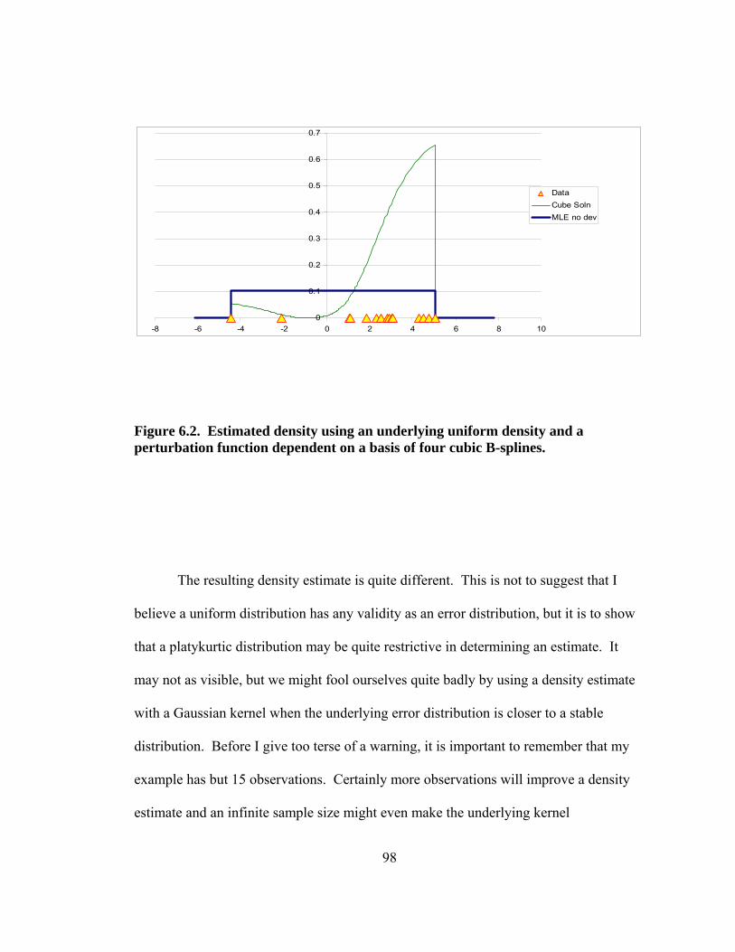
98

0

0.1

0.2

0.3

0.4

0.5

0.6

0.7

-8 -6 -4 -2 0 2 4 6 8 10

DataCube SolnMLE no dev

Figure 6.2. Estimated density using an underlying uniform density and a perturbation function dependent on a basis of four cubic B-splines.

The resulting density estimate is quite different. This is not to suggest that I

believe a uniform distribution has any validity as an error distribution, but it is to show

that a platykurtic distribution may be quite restrictive in determining an estimate. It

may not as visible, but we might fool ourselves quite badly by using a density estimate

with a Gaussian kernel when the underlying error distribution is closer to a stable

distribution. Before I give too terse of a warning, it is important to remember that my

example has but 15 observations. Certainly more observations will improve a density

estimate and an infinite sample size might even make the underlying kernel

99

insignificant, as would a prior distribution of beliefs be seriously less significant to a

Bayesian in view of overwhelming subsequent empirical evidence against those beliefs.

Then what should we do? My advice is to be wary, fit the density to multiple

kernels and carefully assess the risk involved in making any inferences. A stable is not

automatically the answer as it will increase tail probabilities based just as a Gaussian (or

a uniform) will decrease them. At this point I do not have enough evidence to refute

using a Gaussian kernel as Gallant et al. do, but I do think it would be judicious to be

quite cautious with conclusions derived from it, especially those dependent on tail

probabilities. Additionally, analogous to the major premise of this work with regards to

model parameters, any such density estimate will likely fit the data too well, better than

the data fits the true underlying distribution.

6.2 MULTIPLE NON-REJECTIONS

The Lagrange Multiplier tests studied herein are designed to be used with model

parameters and correct for the over-acceptance of any null hypothesis that one finds

with the more naïve GFTs. The tests are not designed to, for example, select between

two or a few competing distributions. If you “know” or wish to choose between two

distributions, it will be better to simply use maximum likelihood as a criteria between

the two with any necessary adjustment if one model has the advantage of more

parameters. If you remain troubled between two or a few distributions, a Bayesian

approach with some weighted average of the competitors might even be reasonable.

It may be better to choose based on some appealing aspects of one distribution

based on theory, economic or probabilistic, or even to employ the most parsimonious

100

model in line with Box and Jenkins original advice on time series or the much earlier

advice in the spirit of Occam’s razor.

Above all, my recommendation would be similar to what was given in the

previous section. Absent compelling statistical or economically theoretical data to the

contrary, be very cautious. Do sensitivity analysis with multiple models to see what

difference the different distributions might make. Although you may have to adjust

critical points if you are employing multiple statistical tests, you do not want your name

on a study that suggests it is not economically efficient to build higher levees around

New Orleans based on a Gaussian kernel without even employing some leptokurtic

alternatives.

101

CHAPTER 7

MEANING OF BASIS VECTORS OF PERTURBATION FUNCTIONS

When Neyman first proposed smooth goodness-of-fit tests, he thought of the

various basis vectors as detecting deviations from the null hypothesized error. He

thought that four or five basis vectors would be sufficient to detect most alternatives.

But what does it mean when a coefficient for a basis vector is not zero? Generally, one

can think of the first polynomial basis vector detecting changes in the location, but there

are some additional deviations as well. A non-zero coefficient attached to the second

polynomial basis vector generally affects the second moment, but here too there some

are additional deviations. In general, much of the deviation associated with non-zero

coefficients in the kth polynomial basis vector is in the kth moment.

Below are visual representations of the effect of non-zero coefficients for the

first eight Neyman-Legendre polynomials has if one was testing the null hypothesis of

an underlying Gaussian distribution. The thickest lines are the Gaussian density; the

medium-thick lines represent the densities with a single positive coefficient for the kth

polynomial basis vector. The thinnest lines represent the densities with a single

negative coefficient for the kth polynomial basis vector.

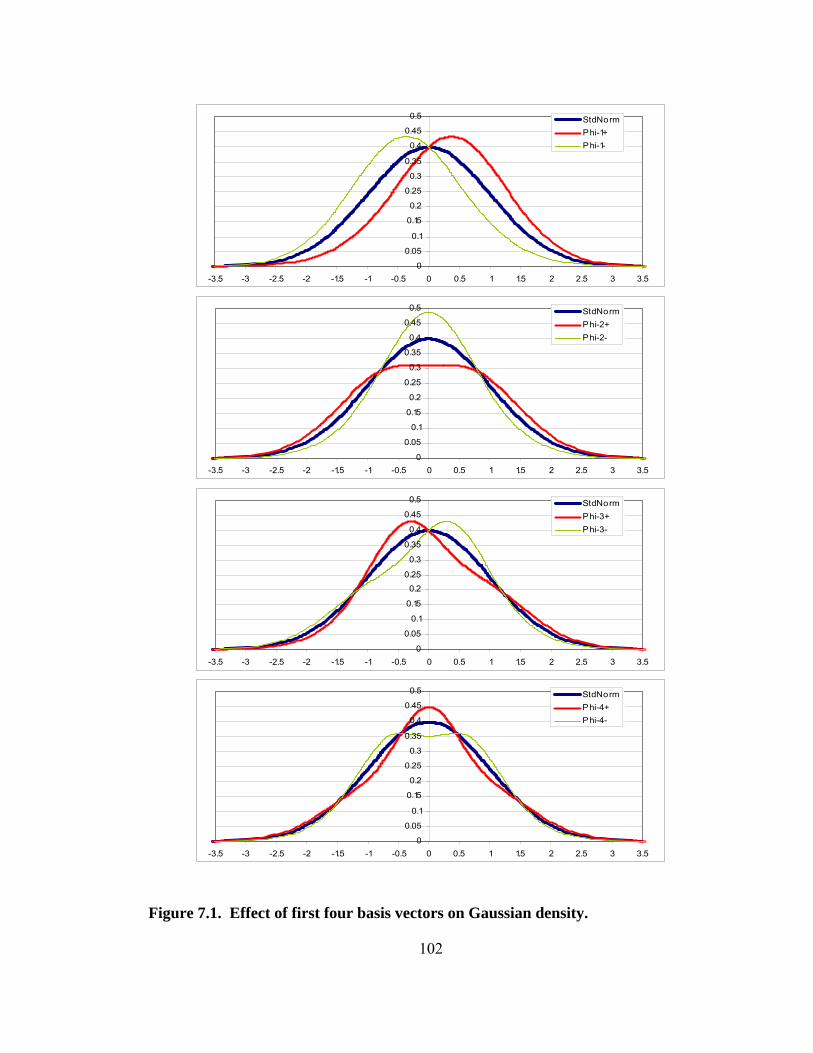
102

0

0.05

0.1

0.15

0.2

0.25

0.3

0.35

0.4

0.45

0.5

-3.5 -3 -2.5 -2 -1.5 -1 -0.5 0 0.5 1 1.5 2 2.5 3 3.5

StdNormPhi-1+Phi-1-

0

0.05

0.1

0.15

0.2

0.25

0.3

0.35

0.4

0.45

0.5

-3.5 -3 -2.5 -2 -1.5 -1 -0.5 0 0.5 1 1.5 2 2.5 3 3.5

StdNormPhi-2+Phi-2-

0

0.05

0.1

0.15

0.20.25

0.3

0.35

0.4

0.45

0.5

-3.5 -3 -2.5 -2 -1.5 -1 -0.5 0 0.5 1 1.5 2 2.5 3 3.5

StdNormPhi-3+Phi-3-

0

0.05

0.1

0.15

0.2

0.25

0.3

0.35

0.4

0.45

0.5

-3.5 -3 -2.5 -2 -1.5 -1 -0.5 0 0.5 1 1.5 2 2.5 3 3.5

StdNormPhi-4+Phi-4-

Figure 7.1. Effect of first four basis vectors on Gaussian density.

103

0

0.05

0.1

0.15

0.2

0.25

0.3

0.35

0.4

0.45

0.5

-3.5 -3 -2.5 -2 -1.5 -1 -0.5 0 0.5 1 1.5 2 2.5 3 3.5

StdNormPhi-5+Phi-5-

-0.1

0

0.1

0.2

0.3

0.4

0.5

0.6

0.7

-3.5 -3 -2.5 -2 -1.5 -1 -0.5 0 0.5 1 1.5 2 2.5 3 3.5

StdNormPhi-6+Phi-6-

0

0.05

0.1

0.15

0.2

0.25

0.3

0.35

0.4

0.45

0.5

-3.5 -3 -2.5 -2 -1.5 -1 -0.5 0 0.5 1 1.5 2 2.5 3 3.5

StdNormPhi-7+Phi-7-

0

0.05

0.1

0.15

0.20.25

0.3

0.35

0.4

0.45

0.5

-3.5 -3 -2.5 -2 -1.5 -1 -0.5 0 0.5 1 1.5 2 2.5 3 3.5

StdNormPhi-8+Phi-8-

Figure 7.2. Effect of basis vectors five through eight on Gaussian density.

104

One can observe from the density affected by the first basis vector that there is

more than a simple shift in location as the maximum height of the density increases,

whether the coefficient is positive or negative. Similarly, in perusing the second graph,

we can see some change in kurtosis rather than just a change in variance. The third and

fourth graphs do exhibit changes in skewness and kurtosis, but something more.

There is a bit of a problem in describing the density changes in the remaining

graphs because we have no standard words for what changes when the 5th through 8th

moments change. The 5th and 7th describe changes that are obviously odd functions; I

suppose we could call these (after skewness) 5-ness and 7-ness or, perhaps, quintness

and septness. The 6th graph is particularly striking, showing waves and four relative

modes for a positive coefficient with three for a negative coefficient. Both the 6th and

8th graphs are even functions so candidate names might be (after kurtosis) 6-tosis and 8-

osis or sextosis and octosis. Certainly, a better linguist might come up with better

names; however, it is helpful to visualize just what types of deviations the different

basis vectors can cause. Of course, linear combinations of them might cause some other

striking densities.

105

CHAPTER 8

TIME DEPENDENT ERRORS Can these types of GFT tests be used with dependent errors with ARMA, ARCH,

GARCH type models?

The short answer is yes, given that maximum likelihood estimation of the model

in question is possible and that the model can be transformed to one with independently,

identically distributed random variables. It is not my intention to prove this, but to give

enough detail to convince the reader of the likely success of proceeding in this

direction, should the situation suggest a time-dependent model.

8.1 EXAMPLES USING TIME SERIES MODELS

Consider a general GARCH(p,q) model:

yt = h(Xt;β) + ηt , t = 1,…,T

where yt is the observed dependent variable at time t, Xt is a row vector of known

constants at time t (and is uncorrelated with ηt ), β is a vector of unknown coefficients,

with function h(Xt;β ) being possibly non-linear;

σ2t = ω + A(L,ξ)η2

t + B(L,ζ )σ2t

where σ2t is the time-varying variance of the innovations, ω > 0, A(L,ξ ) and B(L,ζ) are

lag polynomials with the vectors: ξ and ζ, respectively, having p and q coordinates. For

shorthand in what follows, let λ = (ω, ξ , ζ). Thus, a GARCH(1,1) model would have

σ2t = ω + ξ1η2

t - 1 + ζ1 σ2t – 1.

106

With any GARCH model, ηt = σtεt , with εt ~ IID, mean zero, scale 1, and,

although, it is commonly assumed that εt ~ N(0,1), we can have:

H0: ε t ~ F(z;γ) vs. H1: ε t ~ G(F(z;γ)), independent of t

where G(u) is defined by its density function: g(u) = G'(u) = ( )∑=

+m

jjj u

11 φα .

Presume that one can estimate θ = (β', λ', γ')' of the restricted model indicated by

the null hypothesis by maximum likelihood and form estimates of the ε t for testing.

Depending on the simplicity of the strategy for estimating GARCH models, one can

estimate θ = (β', λ', γ')' of the restricted model indicated by the null hypothesis by

maximum likelihood as follows:

We have estimates of ηt rather than εt, so we need use a change-of-variable

transformation to find the density of the ηt’s. We have

( ) ( ) ( ) ( ) ( )βλσγ

βλση

θηβλση

εβλσ

ηε

,1;

,;~

,1,

, tt

tt

tt

t

t

tt ff

dd

⎟⎟⎠

⎞⎜⎜⎝

⎛=⇒== .

Note: In computing maximum likelihood, not only is σ2t a function of λ = (ω, ξ , ζ), but

it also depends on past values of ηt = yt - h(Xt;β), so it has the parameter β.

So, ( ) ( ) ( ) ( ) ( )βλσγβλσ

ηβλσγ

βλση

η ,ln21;

,ln,ln;

,ln~ln 2

tt

tt

t

tt fff −⎟⎟

⎠

⎞⎜⎜⎝

⎛=−⎟⎟

⎠

⎞⎜⎜⎝

⎛= . Then

the log likelihood function to maximize would be:

( ) ( )( ) ( )∑

=⎥⎦

⎤⎢⎣

⎡−⎟⎟

⎠

⎞⎜⎜⎝

⎛ −=

T

tt

t

tt XhyfXyl

1

2 ,ln21;

,;

ln,; βλσγβλσ

βθ .

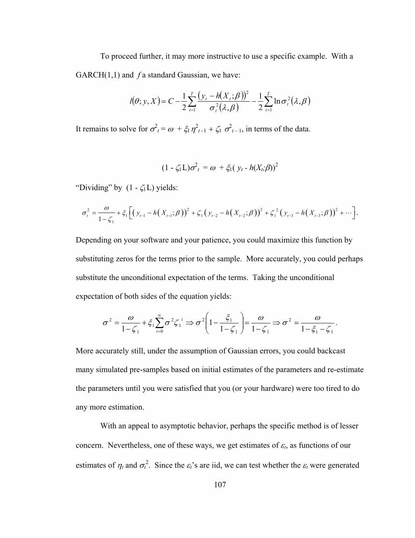
107

To proceed further, it may more instructive to use a specific example. With a

GARCH(1,1) and f a standard Gaussian, we have:

( ) ( )( )( ) ( )∑ ∑

= =

−−

−=T

t

T

tt

t

tt XhyCXyl

1 1

22

2

,ln21

,;

21,; βλσ

βλσβ

θ

It remains to solve for σ2t = ω + ξ1η2

t - 1 + ζ1 σ2t – 1, in terms of the data.

(1 - ζ1L)σ2t = ω + ξ1( yt - h(Xt;β))2

“Dividing” by (1 - ζ1L) yields:

( )( ) ( )( ) ( )( )2 2 22 21 1 1 1 2 2 1 3 3

1

; ; ;1t t t t t t ty h X y h X y h X

ωσ ξ β ζ β ζ β

ζ − − − − − −= + − + − + − +−

⎡ ⎤⎣ ⎦L .

Depending on your software and your patience, you could maximize this function by

substituting zeros for the terms prior to the sample. More accurately, you could perhaps

substitute the unconditional expectation of the terms. Taking the unconditional

expectation of both sides of the equation yields:

11

2

11

121

0

21

1

2

1111

1 ζξωσ

ζω

ζξ

σζσξζ

ωσ−−

=⇒−

=⎟⎟⎠

⎞⎜⎜⎝

⎛−

−⇒+−

= ∑∞

=

i

i

.

More accurately still, under the assumption of Gaussian errors, you could backcast

many simulated pre-samples based on initial estimates of the parameters and re-estimate

the parameters until you were satisfied that you (or your hardware) were too tired to do

any more estimation.

With an appeal to asymptotic behavior, perhaps the specific method is of lesser

concern. Nevertheless, one of these ways, we get estimates of εt, as functions of our

estimates of ηt and σt2. Since the εt’s are iid, we can test whether the εt were generated

108

by our hypothesized distribution, F, or a more general distribution G ° F, by the same

procedures as outlined earlier.

As additional examples, consider an AR(1) model and an MA(1) model:

AR(1): yt = h(Xt;β) + ηt , t = 1,…,T

ηt = ρηt-1 + εt εt iid ~ F

⇒ εt = yt - h(Xt;β) - ρ[ yt-1 - h(Xt-1;β) ]

So you can plug this formula into any likelihood in place of εt and proceed with the

hypothesis test.

MA(1): yt = h(Xt;β) + ηt , t = 1,…,T

ηt = εt -νεt-1 εt iid ~ F

⇒ ( ) ( )( ) ( )( ) L−−−−−−= −−−− βνβνβε ;;; 222

11 ttttttt XhyXhyXhy

So, similar to the GARCH example already shown, a choice must be made about what

to do to estimate data prior to the sample. This simplest assumption, which is not as

bad as in the GARCH example is to assume prior εt = 0, although there are better ways

especially if the estimate of η1 is large in absolute value.

In conclusion, the Lagrange multiplier tests should be applicable in any situation

in which we can isolate independent, identically distributed random variables and we

can make maximum likelihood estimates of the restricted model.

109

8.2 ESTIMATION OF σ1

One can imagine, given infinite computational resources, the estimation of past

ε’s by maximizing ( ) ( )0

0 1 1; , , , , , ; , , , , ,t cond n t tt n

f L y y X Xε γ β λ γ ε ε−=−

⎛ ⎞⎜ ⎟⎝ ⎠∏ K K K over

sequences over past values of ε−n,…, ε0, as n increases, and over the other parameters.

Practically, at some point, N, the estimates of the other parameters would not be

changing much, or at all based on some finite available computational precision. The

ε’s that are sufficiently far in the past will not affect the function enough to make a

difference on the selection of the estimates of the other parameters. Thus, the estimates

for ancient ε’s would effectively be set at the mode of f, since this is its maximal value.

With most error models, the mode is zero. This would suggest that the oldest ε’s would

be near the mode41 and that the more recent ε’s would be more likely to wander away

from the mode to help better explain the error terms early in the data. However, this

will tend to give too close of a fit. To see this, consider the difference between this

method of estimation and a situation in which you are given the past values of ε to be

equal to the estimate. It does not seem correct that you would get the same answers.

In their famous 1970 volume, Box and Jenkins identified, under the assumption

of Gaussian errors, that the covariance structure between εt and εt-k is exactly the same

as the covariance structure between εt and εt+k. This allowed them to posit that if the

series were to run in reverse, the “backcasting” of values occurring prior to the sample

would be accomplished in the same fashion as “forecasting” future values. This would

41 Consider an MA model of low order. In these cases, any ε -k, with k > order would be at the mode and others would be chosen to maximize the function.

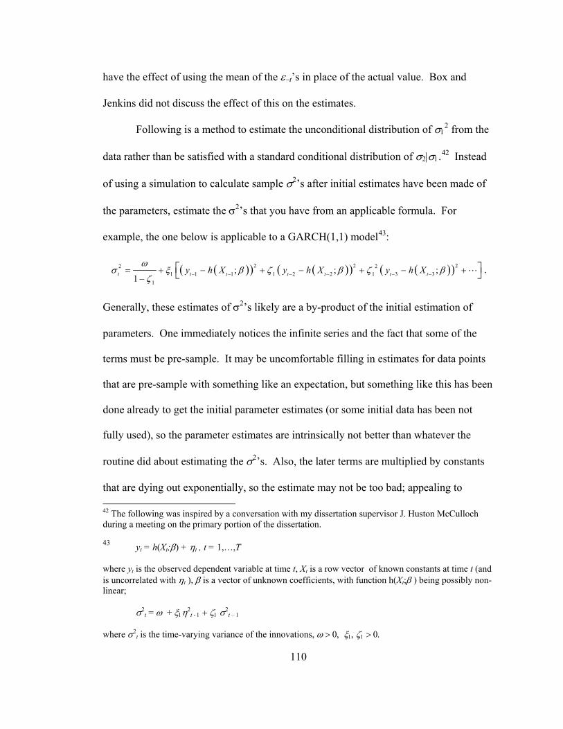
110

have the effect of using the mean of the ε−t’s in place of the actual value. Box and

Jenkins did not discuss the effect of this on the estimates.

Following is a method to estimate the unconditional distribution of σ12 from the

data rather than be satisfied with a standard conditional distribution of σ2|σ1.42 Instead

of using a simulation to calculate sample σ2’s after initial estimates have been made of

the parameters, estimate the σ2’s that you have from an applicable formula. For

example, the one below is applicable to a GARCH(1,1) model43:

( )( ) ( )( ) ( )( )2 2 22 21 1 1 1 2 2 1 3 3

1

; ; ;1t t t t t t ty h X y h X y h X

ωσ ξ β ζ β ζ β

ζ − − − − − −= + − + − + − +−

⎡ ⎤⎣ ⎦L .

Generally, these estimates of σ2’s likely are a by-product of the initial estimation of

parameters. One immediately notices the infinite series and the fact that some of the

terms must be pre-sample. It may be uncomfortable filling in estimates for data points

that are pre-sample with something like an expectation, but something like this has been

done already to get the initial parameter estimates (or some initial data has been not

fully used), so the parameter estimates are intrinsically not better than whatever the

routine did about estimating the σ2’s. Also, the later terms are multiplied by constants

that are dying out exponentially, so the estimate may not be too bad; appealing to 42 The following was inspired by a conversation with my dissertation supervisor J. Huston McCulloch during a meeting on the primary portion of the dissertation. 43 yt = h(Xt;β) + ηt , t = 1,…,T where yt is the observed dependent variable at time t, Xt is a row vector of known constants at time t (and is uncorrelated with ηt ), β is a vector of unknown coefficients, with function h(Xt;β ) being possibly non-linear;

σ2t = ω + ξ1η2

t - 1 + ζ1 σ2t – 1

where σ2

t is the time-varying variance of the innovations, ω > 0, ξ1, ζ1 > 0.

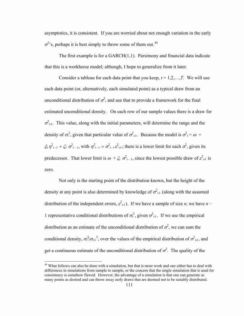
111

asymptotics, it is consistent. If you are worried about not enough variation in the early

σ2’s, perhaps it is best simply to throw some of them out.44

The first example is for a GARCH(1,1). Parsimony and financial data indicate

that this is a workhorse model; although, I hope to generalize from it later.

Consider a tableau for each data point that you keep, t = 1,2,…,T. We will use

each data point (or, alternatively, each simulated point) as a typical draw from an

unconditional distribution of σ2, and use that to provide a framework for the final

estimated unconditional density. On each row of our sample values there is a draw for

σ2t-1. This value, along with the initial parameters, will determine the range and the

density of σt2, given that particular value of σ2

t-1. Because the model is σ2t = ω +

ξ1η2t - 1 + ζ1 σ2

t – 1, with η2t - 1 = σ2

t - 1ε2t-1; there is a lower limit for each σ2, given its

predecessor. That lower limit is ω + ζ1 σ2t – 1, since the lowest possible draw of ε2

t-1 is

zero.

Not only is the starting point of the distribution known, but the height of the

density at any point is also determined by knowledge of σ2t-1 (along with the assumed

distribution of the independent errors, ε2t-1). If we have a sample of size n, we have n –

1 representative conditional distributions of σt2, given σ2

t-1. If we use the empirical

distribution as an estimate of the unconditional distribution of σ2, we can sum the

conditional density, σt2|σt-1

2, over the values of the empirical distribution of σ2t-1, and

get a continuous estimate of the unconditional distribution of σ2. The quality of the

44 What follows can also be done with a simulation, but that is more work and one either has to deal with differences in simulations from sample to sample, or the concern that the single simulation that is used for consistency is somehow flawed. However, the advantage of a simulation is that one can generate as many points as desired and can throw away early draws that are deemed not to be suitably distributed.

112

continuous estimate will be dependent on the quality of the empirical estimate, since the

conditional distributions will be exact (or numerically very close); however, the

continuous estimate will look more like the actual distribution since it will be defined

on an infinite continuous support, the positive real line.

Shown below are pictorial representations of what the individual contributions

to the overall estimate look like for ω = 1, ξ1 = 0.4, ζ1 = 0.2, assuming Gaussian errors.

I have selected densities from the 1st, 25th, 50th, 75th, and 99th percentiles from a sample

of 10,000.

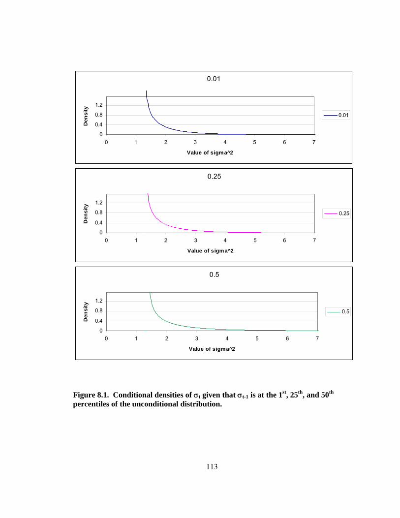
113

0.01

0

0.4

0.8

1.2

0 1 2 3 4 5 6 7

Value of sigma^2

Den

sity

0.01

0.25

0

0.4

0.8

1.2

0 1 2 3 4 5 6 7

Value of sigma^2

Den

sity

0.25

0.5

0

0.4

0.8

1.2

0 1 2 3 4 5 6 7

Value of sigma^2

Den

sity

0.5

Figure 8.1. Conditional densities of σt given that σt-1 is at the 1st, 25th, and 50th percentiles of the unconditional distribution.

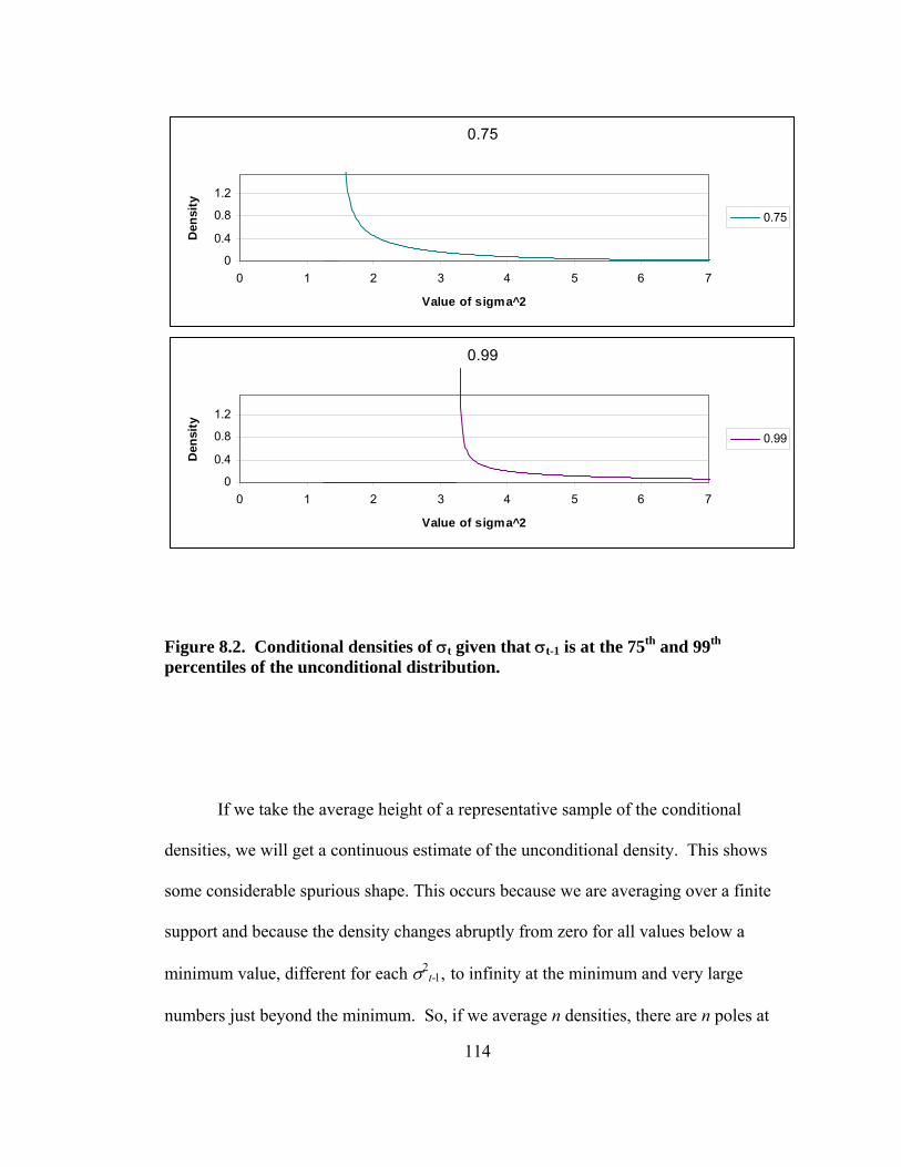
114

0.75

0

0.4

0.8

1.2

0 1 2 3 4 5 6 7

Value of sigma^2

Den

sity

0.75

0.99

0

0.4

0.8

1.2

0 1 2 3 4 5 6 7

Value of sigma^2

Den

sity

0.99

Figure 8.2. Conditional densities of σt given that σt-1 is at the 75th and 99th percentiles of the unconditional distribution.

If we take the average height of a representative sample of the conditional

densities, we will get a continuous estimate of the unconditional density. This shows

some considerable spurious shape. This occurs because we are averaging over a finite

support and because the density changes abruptly from zero for all values below a

minimum value, different for each σ2t-1, to infinity at the minimum and very large

numbers just beyond the minimum. So, if we average n densities, there are n poles at

115

the n minima. Because of that, both smoothing and scaling techniques may be

necessary to make the distribution look differentiable and integrate to unity.

Shown below is what could be called the Density Method, so called since it is

the result of the average of the densities, in this case of the 99 percentiles. So, this is the

result of using 99 out of a possible 10,000 sample σ2t-1’s.

Average - Density Method

0

0.4

0.8

1.2

0 1 2 3 4 5 6 7

Value of sigma^2

Den

sity

Average

Figure 8.3. Sum of 99 conditional densities to approximate the unconditional density.

This can be improved upon greatly by using a Distribution Method, with the

same sample points, but averaging the cdf rather than the pdf. This is because the

116

distribution is continuous, although its derivative fails to exist at the n poles of the

density. Then the density, using the Distribution Method, is calculated by taking central

differences at each point of evaluation.

Average - Distribution Method

0

0.4

0.8

1.2

0 1 2 3 4 5 6 7

Value of sigma^2

Dis

trib

utio

n

Average

Figure 8.4. Sum of 99 conditional cdfs to approximate the unconditional cdf.

It is still the case that the density does not exist at the poles, but since I am

taking central differences around each pole, I am getting a fairly poor numerical

estimate of the derivative, which happens to be closer to the density for values outside

the immediate neighborhood of the poles. In this case, two wrongs make it look right.

However, the smooth parts of the graph are slightly too low to be the unconditional

117

density, whereas the volatile spikes upward are too high when compared with the

unconditional density.

Average - Distribution Method

0

0.4

0.8

1.2

0 1 2 3 4 5 6 7

Value of sigma^2

Den

sity

Average

Figure 8.5. Unconditional density derived from unconditional cdf.

Because of the special selection of points, it would be unrealistic to get such a

good representation if the sample size is only 99; however, the estimate is still fairly

accurate as is shown by the chart below which uses the last 99 points of the sample of

10,000. The chart is bigger, because the differences would be less detectable on a

smaller scale.

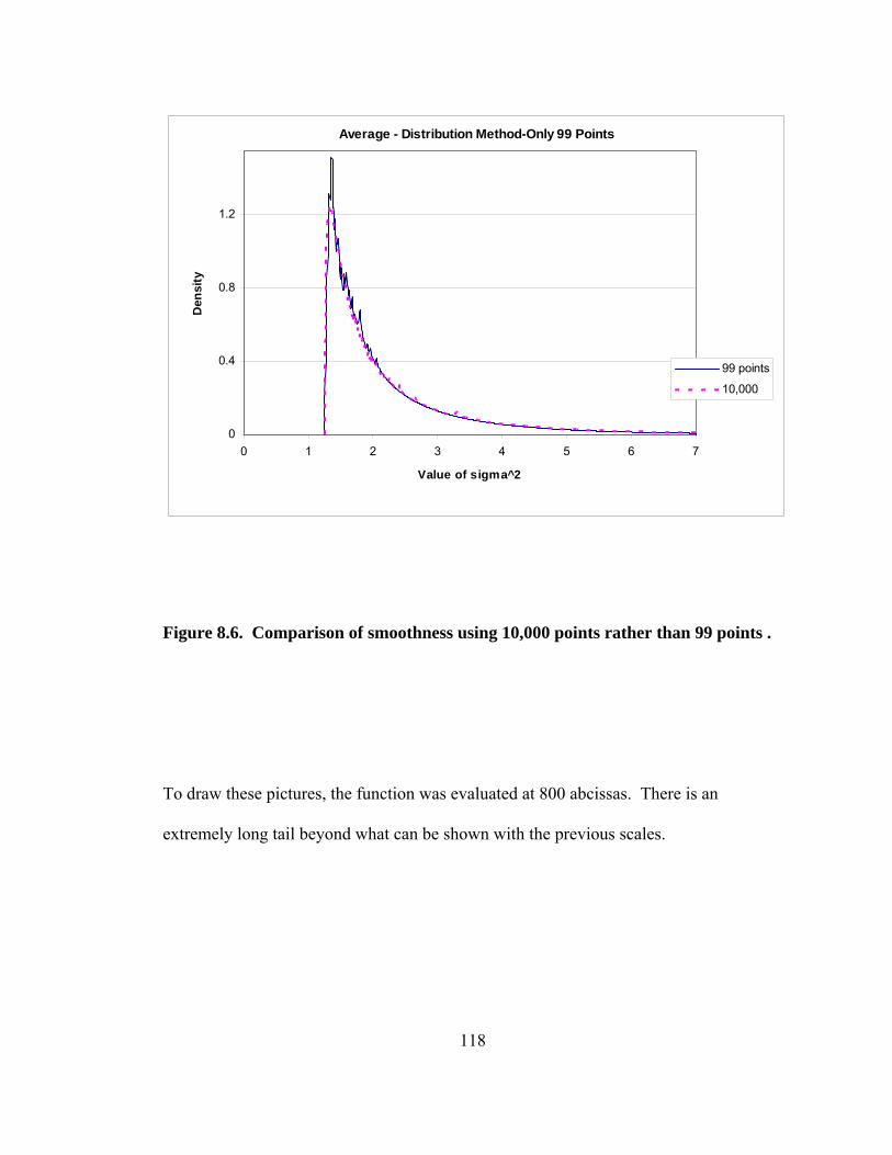
118

Average - Distribution Method-Only 99 Points

0

0.4

0.8

1.2

0 1 2 3 4 5 6 7

Value of sigma^2

Den

sity

99 points

10,000

Figure 8.6. Comparison of smoothness using 10,000 points rather than 99 points .

To draw these pictures, the function was evaluated at 800 abcissas. There is an

extremely long tail beyond what can be shown with the previous scales.

119

Tail - Distribution Method

0

0.0020.004

0.0060.008

0.01

7 8 9 10 11 12 13 14 15 16 17 18 19 20 21 22 23 24 25

Value of sigma^2

Den

sity

Average

Figure 8.7. Upper tail of unconditional distribution of σ .

With either method, the unconditional density of σ2 can be determined at as

many or as few points as desired by the practitioner by the use of a formula. Shown

below is the formula for the density:

( )( ) 1

2

1 12

1

1

12

20

1,

~

1ζ

ωσζωσξ

ξζωσ

σ−

>−−

⎟⎟

⎠

⎞

⎜⎜

⎝

⎛ −−

= ∑=

n

i ii

i

i

uu

uu

f

nh , where

( ) ( )⎩⎨⎧ −<

=otherwiseuf

zf i

0~ 2

1 ωσζε and ui is the ith realization from the sample of σ2 standing

in for the values of σ2t-1. If you deem the sample to be too small to suitably estimate the

unconditional density, one could select n1 equally spaced quantiles from h0, and

120

substitute them into the formula above as values of u (using n1 instead of n), to get a

perhaps smoother estimate h1(σ2).

Where does this formula come from and can it be generalized to GARCH(p,q)

and ARCH(p) models? The answer to the latter question is “yes” and its explanation

will be deferred. For the answer to the former, proceed.

The model for GARCH(1,1) is σ2t = ω + ξ1η2

t - 1 + ζ1 σ2t – 1, with

η2t - 1 = σ2

t -1ε2t-1. To proceed with a formula, there must be an assumption that the

distribution of εt-1 ~ f (0,1) for some function where, WLOG, the location and scale

parameters can be set to zero and one, respectively, by the presence of a location

parameter in the model and by scaling of σ2t-1. Since the ε ’s are independent, the time

subscript can be dropped in the expressions that presently follow.

The conditional distribution of σ2t | σ2

t-1 is the constant ω + ζ1 σ2t – 1 plus the

random variable, ε2, scaled by ξ1σ2t – 1. Whenever we know the density of ε2, which

we will know if we know the density of ε , we will know the conditional density of σ2t

| σ2t-1.

With the common assumption of Gaussian errors, we know that ε2 ~ χ2(1). If

we assume ε ~ f (0,1) with support (-∞,∞), then, through transformation of variables, we

know the density, g, of ε2 is ( ) ( ) ( )[ ]22

2

2

21 εεε

ε ffg +−= on (0,∞). If f is

symmetric, then, simply, ( ) ( )2

22

ε

εε fg = on (0,∞). If we let u be a particular value of

σ2t-1, then with one more transformation, ε2 = (σ2

t - ω − ζ1 u) / ξ1u, dε2/dσ2t = 1 / ξ1u,

121

we get the conditional density ( )( ) ⎟⎟

⎠

⎞⎜⎜⎝

⎛∞

−∈

−−

⎟⎟

⎠

⎞

⎜⎜

⎝

⎛ −−

= ,1

,|1

2

12

1

1

12

2

ζωσ

ζωσξ

ξζωσ

σuu

uuf

uh . Up

to this point, the density is exact; there has been no estimation. The estimation appears

when we substitute the empirical distribution of σ2 for the unconditional distribution for

u (= σ2t-1 ). Summing over the n points and multiplying by the probability of each

point, 1/n in the empirical distribution, we get the formula indicated earlier.

This formula is perfectly general. We can eliminate one of the transformations

if we know the distribution of ε2 in addition to knowing the distribution of ε. In the

examples that follow, let y = ε2 for ease of notation:

If ε is Cauchy, ( )( ) yy

yg+

=1

1π

; if ε is Student-t, ( ) ( )( ) ( ) 2

1

2

21

1+

+

+Γ

Γ= r

ryr

r

yryg

π; if ε is

G.E.D., ( ) ( ) ⎟⎟⎠

⎞⎜⎜⎝

⎛−

Γ=

−22

1

1exp

2

α

α

α yyyg . Even if we cannot write down the density as in

the case of the symmetric stable distribution, if we can numerically determine the

density, we can numerically determine the density of the random variable that is the

square: ( ) ( )yyf

yg = for symmetric densities and ( ) ( ) ( )[ ]yfyfy

yg +−=2

1 for

non-symmetric. In all the foregoing cases, the support for y is (0,∞).

So, this formula works for many error functions. How can we generalize to

other GARCH models? It turns out that the generalization for more “GARCH”

(variance) terms is easier than the generalization for more “ARCH” (innovation) terms,

122

so I will start with the “GARCH” generalization. To begin with, what if there are zero

variance terms and 1 ARCH term?

The formula just reduces to:

( )( )

ωσωσξ

ξωσ

σ >−

⎟⎟⎠

⎞⎜⎜⎝

⎛ −

= ∑=

2

12

1

1

2

20 ,

~

1 n

i i

i

u

uf

nh

With q GARCH terms and 1 ARCH term, the formula becomes:

( ) ( ) ∑∑

∑

∑

=

+−

=

=

=

−>

⎟⎟⎠

⎞⎜⎜⎝

⎛−−

⎟⎟⎟⎟⎟

⎠

⎞

⎜⎜⎜⎜⎜

⎝

⎛−−

−−= q

kk

qn

i q

kikki

q

kikk

uu

u

uf

qnh

1

21

1

1

211

11

1

2

20

1,

~

11

ζ

ωσ

ζωσξ

ξ

ζωσ

σ , where uik =

σ2i,t-k and ( ) ( )

⎪⎩

⎪⎨⎧

−<= ∑=

otherwise

ufzfq

kkk

0

~ 2

1ωσζε . This expansion is accomplished essentially

by placing the sum of all the GARCH terms where the first term was in the previous

formula.

In this case, we are first finding an exact representation of the conditional

distribution of σ2t | σ2

t-1, σ2t-2, …, σ2

t-q and then using the n – (q - 1) sequences of {σ2t-1,

σ2t-2, …, σ2

t-q} that we have in the sample:

{σ2q, σ2

q-1, …, σ22, σ2

1}, {σ2q+1, σ2

q, …, σ23, σ2

2},…{σ2n, σ2

n-1, …, σ2n-q+1}, so

as to preserve the potential relationships between consecutive σ2’s, and serve as an

empirical estimate of the distribution of the q-tuple, (σ2t-1, σ2

t-2, …, σ2t-q).

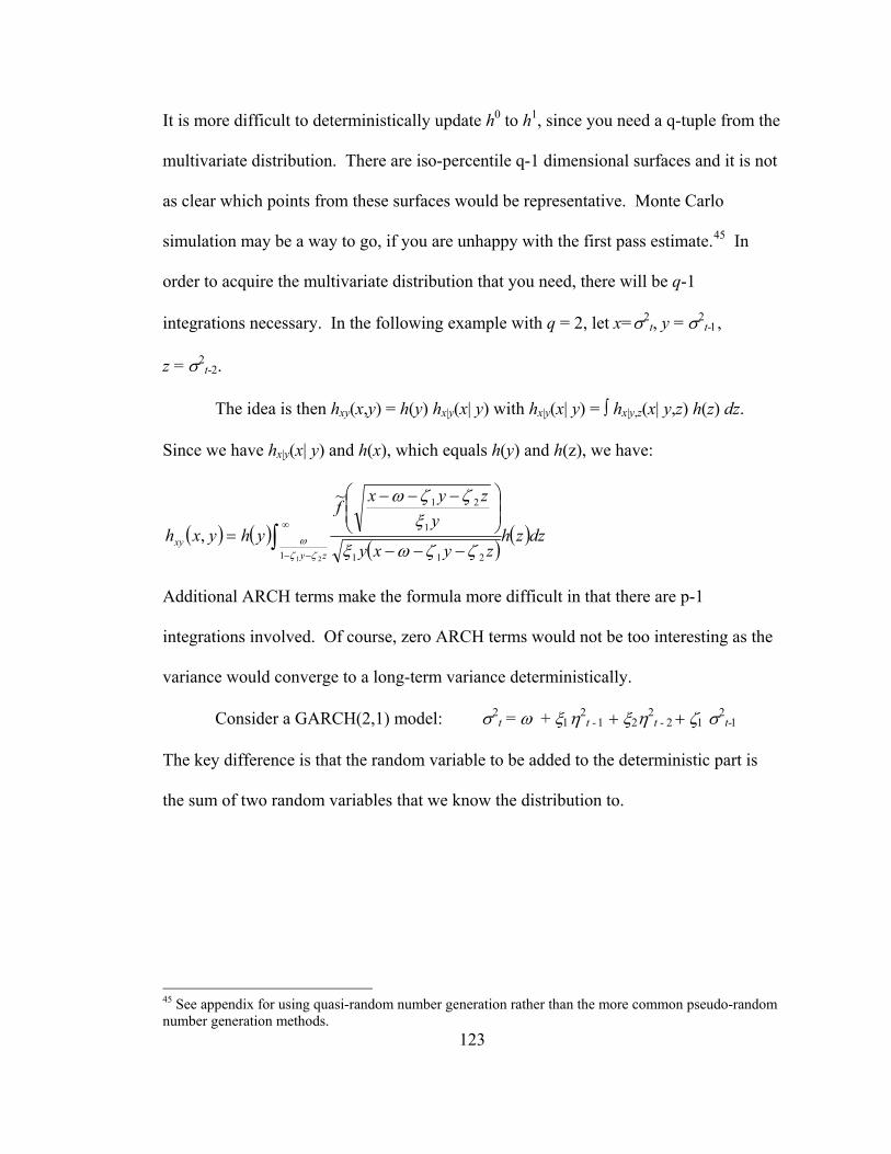
123

It is more difficult to deterministically update h0 to h1, since you need a q-tuple from the

multivariate distribution. There are iso-percentile q-1 dimensional surfaces and it is not

as clear which points from these surfaces would be representative. Monte Carlo

simulation may be a way to go, if you are unhappy with the first pass estimate.45 In

order to acquire the multivariate distribution that you need, there will be q-1

integrations necessary. In the following example with q = 2, let x=σ2t, y = σ2

t-1,

z = σ2t-2.

The idea is then hxy(x,y) = h(y) hx|y(x| y) with hx|y(x| y) = ∫ hx|y,z(x| y,z) h(z) dz.

Since we have hx|y(x| y) and h(x), which equals h(y) and h(z), we have:

( ) ( )( )

( )dzzhzyxy

yzyxf

yhyxhzy

xy ∫∞

−− −−−

⎟⎟⎠

⎞⎜⎜⎝

⎛ −−−

=211 211

1

21~

,ζζ

ωζζωξ

ξζζω

Additional ARCH terms make the formula more difficult in that there are p-1

integrations involved. Of course, zero ARCH terms would not be too interesting as the

variance would converge to a long-term variance deterministically.

Consider a GARCH(2,1) model: σ2t = ω + ξ1η2

t - 1 + ξ2η2t - 2 + ζ1 σ2

t-1

The key difference is that the random variable to be added to the deterministic part is

the sum of two random variables that we know the distribution to.

45 See appendix for using quasi-random number generation rather than the more common pseudo-random number generation methods.

124

Given f as the pdf of ε, we have the pdf of z1 = ξ1η2t - 1, with u1 = σ2

t-1, to be

( )111

11

1

11 zu

uzf

zgξ

ξ ⎟⎟⎠

⎞⎜⎜⎝

⎛

= and the pdf of z2 = ξ2η2t - 2, with u2 = σ2

t-2, to be

( )222

22

2

22 zu

uz

fzg

ξ

ξ ⎟⎟⎠

⎞⎜⎜⎝

⎛

= , both on the support (0,∞). The density of the sum is obtained

along with a nuisance random variable by a two-dimensional bijective transformation,

11011

22

211

22

211 =−

=⇒⎭⎬⎫

=−=

⇒⎭⎬⎫

=+=

Jyz

yyzzy

zzy

We get ( ) ( ) ( ) ∞<<<−= 12222112112 0,, yyygyygyyφ . To get the distribution

that we are interested in, we must integrate out y2, so

( )( )∫

⎟⎟⎠

⎞⎜⎜⎝

⎛

−

⎟⎟⎠

⎞⎜⎜⎝

⎛ −

= 1

0 2222

22

2

2111

11

21

11

ydy

yu

uy

f

yyu

uyy

fy

ξ

ξ

ξ

ξφ

One more transformation from y1 to σ2 yields a formula for GARCH(2,1).

( )( )

21 1

21 1 2 2

1 1 1 2 20 220 21 2 2 21 1 1 1 2

2

1

1 ,1

1

i

i

n iu i

i ii i

u y yf fu uh dy

n u yu u y

σ ω ζ

σ ω ζξ ξ

σξξ σ ω ζ

ωσζ

− − −

=

⎡ ⎤⎛ ⎞− − − ⎛ ⎞⎢ ⎥⎜ ⎟ ⎜ ⎟⎜ ⎟ ⎜ ⎟⎢ ⎥⎝ ⎠ ⎝ ⎠= ⎢ ⎥− ⎢ ⎥− − −

⎢ ⎥⎢ ⎥⎣ ⎦

>−

∑ ∫

%

where ( ) ( )⎩⎨⎧ −<

=otherwiseuf

zf0

~ 211 ωσζε

. The integral in general must be evaluated

numerically.

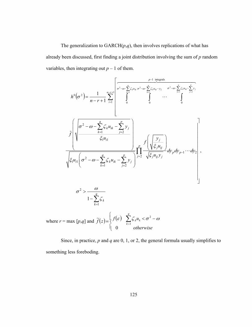
125

The generalization to GARCH(p,q), then involves replications of what has

already been discussed, first finding a joint distribution involving the sum of p random

variables, then integrating out p – 1 of them.

( ) ∑ ∫ ∫ ∫+−

=

−

−− −−− −−−

⎢⎢⎢⎢⎢⎢⎢

⎣

⎡

∑ ∑ ∑∑

+−=

= = ==1

1

integrals 1

0 0 0

201

22

1

2

21

2

11 rn

i

p

u yu yuq

kikk

q

kikk

p

jj

q

kikk

rnh

4444444 84444444 76

L

ζωσ ζωσ ζωσ

σ

2

1 2

1 1

1 222

1 11 2

2

1

,

1

q p

k ik jk j

i j

p j ijp p

q p j j ij ji k ik j

k j

q

kk

u yf

u yf

udy dy dy

u yu u y

σ ω ζ

ξξ

ξξ σ ω ζ

ωσζ

= =

−=

= =

=

⎤⎛ ⎞⎥⎜ ⎟− − −⎥⎜ ⎟⎥⎜ ⎟ ⎛ ⎞ ⎥⎜ ⎟ ⎜ ⎟ ⎥⎜ ⎟ ⎜ ⎟

⎝ ⎠ ⎝ ⎠ ⎥⎥⎛ ⎞⎥− − −⎜ ⎟⎜ ⎟ ⎥⎝ ⎠⎥⎥⎥⎦

>−

∑ ∑

∏∑ ∑

∑

%

L

where r = max [p,q] and ( ) ( )⎪⎩

⎪⎨⎧

−<= ∑=

otherwise

ufzfq

kkk

0

~ 2

1ωσζε

Since, in practice, p and q are 0, 1, or 2, the general formula usually simplifies to

something less foreboding.

126

CHAPTER 9

TEST RECOMMENDATIONS FOR FINANCIAL DATA

This paper introduces a wide range of goodness-of-fit tests. One of the

reasonable questions that can be raised is, “Which one of these tests should be used in a

particular study?” Criteria that might be selected for determining the best test to use are

size distortion and power against likely prescribed alternatives.

As an example, we have tested the proposed econometric goodness-of-fit tests

on the residuals of monthly stock market returns with empirically determined

parameters. Different practitioners have proposed stable, Student-t, GED, and a

mixture of normal distributions to fit the leptokurtosis that prevents the Gaussian

distribution from adequately explaining the residuals. Those past presumptions fueled

the choices of distributions selected.

The empirically determined parameters for the four distributions, using

maximum likelihood estimation, in looking at log excess real monthly returns January,

1953, through December, 2002, were as follows46:

Symmetric stable: α = 1.8622, ln scale = 1.0239, δ = 0.5846

46 These estimates were determined by an adapted Broyden-Fletcher-Goldfarb-Shanno method which was a constrained search over the parameter spaces. Special attention must be given to preventing a routine to go beyond 2 in its search for alpha in a stable distribution or beyond 0 and 1 in its search for p in a mixture of two Gaussians. In addition special routines had to be developed to obtain fast accurate densities for the GED, generalized Student-t, and mixture of two Gaussians. McCulloch’s SYMSTB software, described in "Numerical Approximation of the Symmetric Stable Distribution and Density," in Adler et al. was employed to obtain densities for the symmetric stable case.

127

Generalized student: degrees of freedom = 6.8640, ln scale = 1.2931, mean = 0.6410

Generalized error distribution (GED): power = 1.4187, ln scale = 1.5679, mean =

0.6700

Mixture of Two Gaussians: probability of first standard deviation = 0.9059,

ln(first st. dev.) = 1.3084, ln(second st. dev.) = 2.1247, mean = 0.5935

These were the values used in some simulations for either null hypotheses or

simple alternative hypotheses. It is important to note that the conclusions to be drawn

from this U.S. equities market example may not be applicable in other arenas, although

this example is certainly represented by a broad expanse of literature.

The size distortion and power against the other distributions have been tested for

each of the four leptokurtic distributions.

All sizes and powers are based on simulations using 1000 draws from the Kiss

monster random number generator, described in more detail in the Appendix. All data

is generated based on the empirical market parameters under the assumptions that the

log excess returns were generated by one of the four hypothesized distributions. There

are two test sizes investigated for each scenario, 0.10 and 0.05. There are from 1 to 20

basis parameters tested, 3 to 20 for the Cubic Splines.

Six sample sizes were tested, 31, 100, 316, 1000, and 3162 and 10,000 (10k, k =

3/2 , 2, 5/2 , 3, 7/2 , 4). We tested the size distortion for each Model-Parameter-sensitive

(referred to as “corrected”) goodness-of-fit test and did the same using conventional

(referred to as “naïve”) tests.

There are 18 power tests per null hypothesis, based on 6 possible sample sizes

with 3 possible alternative hypotheses. For each category there is a size-adjusted power

128

for the corrected tests and non-adjusted powers for both the corrected tests and the naïve

tests.

Two types of bases were used to determine goodness-of-fit parameters: the

Cubic Spline basis and the Neyman-Legendre basis. Based on previous samples, the

conclusion was reached that the Neyman-Legendre polynomial basis and the Cubic

Spline basis generally outperformed the other bases investigated (Pearson, the

Quadratic Spline and the Linear Spline). So, in the interest of spending more time on

additional repetitions in the simulations rather than more time on bases that will not be

recommended, only the former two bases are investigated here.

9.1 SIZE DISTORTION

There is tremendous size distortion with the naïve tests in every instance for

every level of parameters. This distortion does not go away as the sample size increases

from 32 to 10,000. It diminishes somewhat as the number of basis parameters goes up,

but this is still not very helpful. The distortion is in the direction of over-acceptance.

For the corrected tests, there is initial size distortion, generally much smaller

than the naïve tests. The size distortion vanishes, within sampling error, for moderate

sample sizes. For some of the largest samples of 10,000, calculation error seems to

have crept in, magnified as the number of basis parameters increases, first with the

Neyman-Legendre basis then with Cubic Spline basis. This was not entirely

unexpected with the Neyman-Legendre basis as rounding errors had been identified

earlier. It is our belief that calculation of the test statistics by quadrupling the number

of intervals for numeric integration would mitigate these errors although that is

unknown at this time due to the tremendous amount of time that each simulation takes.

129

If this presumption is correct, the tests would continue to work well for small number of

parameters and very large sample sizes. The test itself can easily quadruple or increase

by 16-fold the number of intervals when a single calculation is performed; however, the

multiplicity required by all the simulation possibilities makes each new check quite

formidable in terms of time.

For the mixture and as little as 100 observations, with up to 6 basis variables, the

size distortion is undetectable. For 316 observations and the level 0.10 test, most all the

basis parameters are just barely in the low end of the confidence interval. For 1000 and

more observations, there is no discernible distortion.

Distortion gradually disappears for the stable null from 316 to 1000 as well,

although it is small for smaller sample sizes with small numbers of basis parameters as

well. For Student nulls, distortion dies out at only 100 observations. GED nulls require

around 316 observations.

9.2 POWER

The over-acceptance caused by the size distortion in the naïve tests contributes

to poor power against the chosen nulls. With the naïve tests, fitting the model

parameters biases against rejecting any false hypotheses. Hence, practitioners may all

too often mistakenly conclude that, since their test does not reject an alternative

hypothesis, they are justified in accepting the validity of the assumptions in their study.

The naïve tests have power even less than the test size for sample sizes that are quite

high!

The corrected tests do have more power than the naïve tests. However, for small

sample sizes, even with the corrected tests, it is quite difficult to tell these leptokurtic

130

distributions from one another. The positive thing about this is that when the sample

size is high enough for there to be reasonable levels of power (4 to 5 times the test size),

there is negligible size distortion. This means that, in the cases investigated, a user of

this test would not have to go through the trouble of size-adjustment, which means no

lengthy simulations are necessary!

Recommendations can be made based on the null hypothesis chosen, since the

null will be known by the user. There are significant power gains to be made by giving

different recommendations for different nulls, so that is what is done below.

9.3 WITH A STABLE NULL

A GED distribution can start to be detected with as little as 316 observations.

By this time, it is also clear that a pattern which has a power peak at only 2 model

parameters (3 for the Spline). This power peak also works well for “seeing” a Student.

The mixture, with its extra parameter, is quite difficult to identify requiring more than

3000 observations, even to get modest 30% power levels. At 10,000 observations the

most power comes from a large number of parameters. But at 10,000 observations, any

number of parameters (more than 2) will have the same (100%) power levels for the

less leptokurtic random variables. At this number, it is recommended to use the Cubic

Spline, perhaps with 15 parameters, because it has fewer numerical difficulties than the

Neyman as the number of parameters increases.

Included are three of many possible graphs to make that illustration. Others are

included in Appendix I. These graphs represent sample sizes of 316 (105/2) observations

with a stable null hypothesis, at a test size of α = 0.10, using the values for parameters

equal to what was stated at the beginning. The first graph shows that there is negligible

131

size distortion for the corrected test, using 1000 simulations. This is determined

because the corrected test statistics, shown by dark blue diamonds and pink squares, lie

mostly in a 95% confidence interval around 0.10 ( )( )⎟⎟⎠

⎞⎜⎜⎝

⎛±

10009.01.096.110.0 . The 95%

confidence interval is shown by dashed gray lines that are just slightly higher than 0.08

and lower than 0.12.

Actual Size and 95% Conf Limits around 0.10Stable, 316 observations, 0.10 test

0

0.020.040.060.08

0.10.12

0.14

0 5 10 15 20

P arameters

NActual SizeL LimitU LimitSActual SizeNNeymanNSpline

Figure 9.1. Empirical size of 0.10 tests using the naïve and corrected Cubic Spline and Neyman GFTs using numerical quadrature.

This low size distortion of the corrected tests can be contrasted with the

significant size distortion of the naïve tests, shown by the green and orange “×’s.”

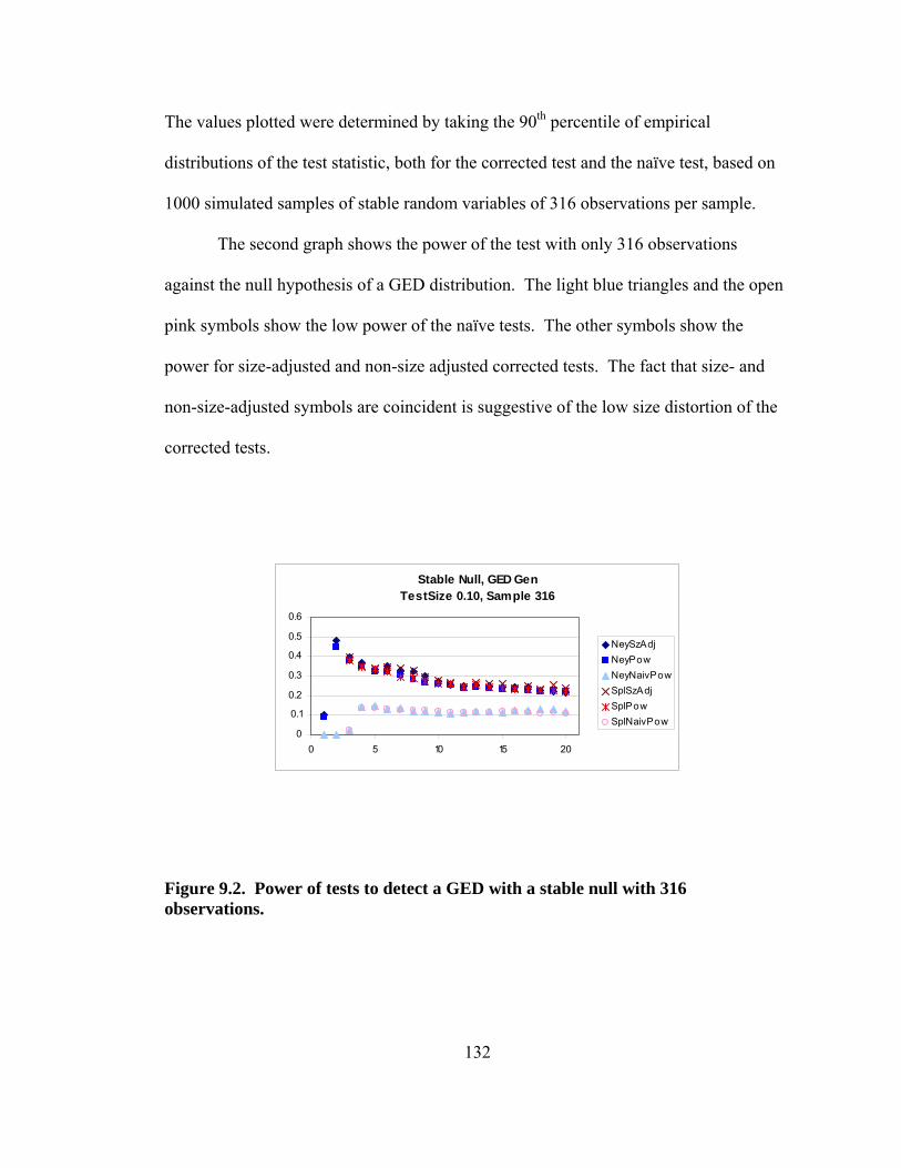
132

The values plotted were determined by taking the 90th percentile of empirical

distributions of the test statistic, both for the corrected test and the naïve test, based on

1000 simulated samples of stable random variables of 316 observations per sample.

The second graph shows the power of the test with only 316 observations

against the null hypothesis of a GED distribution. The light blue triangles and the open

pink symbols show the low power of the naïve tests. The other symbols show the

power for size-adjusted and non-size adjusted corrected tests. The fact that size- and

non-size-adjusted symbols are coincident is suggestive of the low size distortion of the

corrected tests.

Stable Null, GED GenTestSize 0.10, Sample 316

0

0.1

0.2

0.3

0.4

0.5

0.6

0 5 10 15 20

NeySzAdjNeyPowNeyNaivPowSplSzAdjSplPowSplNaivPow

Figure 9.2. Power of tests to detect a GED with a stable null with 316 observations.

133

The next graph shows the power gains when the sample size is increased from

316 observations to 1000 observations.

Stable Null, GED GenTestSize 0.10, Sample 1000

0

0.2

0.4

0.6

0.8

1

0 5 10 15 20

NeySzAdjNeyPowNeyNaivPowSplSzAdjSplPowSplNaivPow

Figure 9.3. Power of tests to detect a GED with a stable null with 1000 observations.

For the rest of the null hypotheses, recommendations about number of basis

parameters are given.

9.4 WITH A STUDENT-T NULL

A stable distribution can be seen almost half the time with 316 observations.

Just about any number of parameters (greater than 2) will work equally effective. GED

and mixtures are still concealed for the most part at this observation level, but a test

with 2 or 3 parameters has the best chance of finding them. So, if a Student is your null,

go with 2 or 3 parameters, regardless of sample size.

134

9.5 WITH A GED NULL

GED’s magic number is 4 parameters. The smallest 3 bases have really bad

power; then, there is a tremendous increase at 4, with ever so little decreases after that.

9.6 WITH A MIXTURE NULL

Unless you have at least 2000 observations, there is no reason to try to test

against the other three possibilities. The mixture pattern seems to be a bit different in

that higher numbers of parameters seem to yield more power. For this reason, the

Cubic Spline is recommended here to avoid numerical inaccuracy, with about 15

parameters. At 10,000, even with the possible inaccuracies, the test with 8 parameters

seems to have fairly low distortion levels, so it would be safe to use against the chosen

alternatives.

9.7 BASIS SIZE VS. SAMPLE SIZE

The original thought was that, in searching for a test with maximal power, one

might find some relationship between the number of basis vectors, m, and the sample

size, n, such as m ∝ n1/2 or m ∝ n2/5. Whereas, it is still the belief that m can increase

with n, I now believe this increase in m will either terminate or plateau and then proceed

quite slowly until n achieves a level high enough to allow for identification of a nonzero

α for the next-highest basis vector. This relationship is highly dependent on the

relationship between a particular null hypothesis and the underlying error distribution.

For a particular underlying error distribution and null hypothesis, the test as

proposed determines the gradient at α=0 towards a vector α∗ = (α1, α2, … , αm),

135

different than a zero vector, which, along with the choice of basis functions, in a sense

identifies the best alternative density in the set of alternative hypotheses.

With some sets of basis vectors and a given sample size, it may be the case that

a test with a subset of the basis vectors is more powerful than the entire set of basis

vectors. Let me illustrate that. The typical test is equally sensitive in each of the m

dimensions, so it will reject the null hypothesis in the event that (a12 + a2

2 + … + am2)1/2

> λm, where the ai’s are estimates for the αi’s. If, for example, it was known that αm = 0,

then the (m – 1)-order test which would reject in the event that (a12 + a2

2 + … + am-12)1/2

> λm-1. Since λm-1 < λm, the (m - 1)-order test would then be more sensitive to

deviations from zero of the remaining α’s, (α1, α2, … , αm-1). Note that if αm is not near

zero then it is possible that the larger set of basis vectors will provide the more powerful

test.

Given a particular underlying distribution (with the data already transformed

based on a particular null hypothesis) and a particular set of basis functions Φ, one

could imagine an infinite α−vector such that α'Φ was equal to the function that is the

correct alternative to the uniform distribution. If for example, the basis functions were

orthogonal polynomials and the underlying density was a polynomial of degree r

transformation of the null density, the length of the α−vector could be shortened to r,

with all ordinates greater than r being zero.

My supposition is that if the alternate density can be exactly represented by a

finite set of the basis functions, r, then regardless of how large n gets, there should not

be additional power gained by increasing the level of m beyond r.

136

If one could then imagine a sample of size n being drawn from this alternate

density, to the extent that n is small, sample error could mask the identity of the true

underlying density. As n gets larger, the sample will get closer and closer to mirroring

the true density.

Allow me to draw an admittedly imperfect analogy. In a footnote, I will note

some of the imperfections with some solutions, but the analogy is clearer without these

complications. Presume a simple polynomial basis with a sample size of n independent

draws from an alternative density. There should be some analogy to the rejection of the

null hypothesis in favor of the alternative hypothesis and the identification of a nonzero

coefficient in a related regression.

If the sample was drawn from the null hypothesis density, the expected values of

the order statistics would be i/n+1, , i = 1,2, …, n. Hence, one could reasonably write

y(i) = i/n+1 + εi.47

So one could test the null hypothesis by performing a regression, using the

ordered transformed sample, y(1) , y(2) , … , y(n) as regressands and the series 1/n+1, 2/n+1,

… , n/n+1 as the related regressors, xi, i = 1,2, …, n, in a model such as:

y(i) = β0xi + β1xi2 + β2xi

3 + …+ βmxim+1 + εi

with the goal to identify nonzero β’s (or a β0 ≠ 1). If n is too small, even if all of the β’s

with positive indices are nonzero, we may not be able to identify all of them (or perhaps

47 One of the imperfections with this analogy is that the εi’s are not independent and are heteroskedastic. One can remove the independence problem by imagining n draws each from n independent samples, then selecting y(i) from the ith sample, i = 1,2, …, n. The y(i)’s will still have different variances, however, these differences can be accommodated by a properly weighted regression technique. In fact a single sample can be used by noting and adjusting for the covariances between these order statistics.

137

any of them) as being more than a couple standard deviations from zero. This would be

analogous to finding α’s different than zero in the primary problem.

With some samples one might identify a β as properly being nonzero, while in

other ones this will go unnoticed. As n increases, depending on the size of β, there will

be a greater and greater chance of it being identified as nonzero, but this indicates an

increase in power as n increases for a fixed level of m, not an indication that m should

increase in proportionally to some fractional power of n.

If the density could be represented by the sum of r products (α1φ1 + α2φ2 + … +

αrφr) with r < m, the test that one of the m β’s would be nonzero would be less powerful

than fitting an r-degree polynomial and testing whether one of the first r β’s were zero.

For smaller sample sizes, even if it takes r basis vectors to exactly fit the

alternate density, a basis with fewer than r elements may be appropriate, if the nonzero

β’s with degree less than r, can be shown to be non-zero more easily by a lower-order

test.

If the alternate density could not be fit exactly by a combination of any finite

number of basis vectors, then m could grow without bounds, but it might grow quite

slowly if some of the later α’s are quite close to zero. In the regression case, we might

even be able to identify the proportion of times that a βj would be identified as non-

zero, based on the value of its standard deviation, the jth diagonal element in a σ2( X 'X) -1

matrix with known X ' = (1/n+1, 2/n+1, … , n/n+1) (or a suitable estimate of the variance-

covariance matrix given a weighting matrix).

138

Although the regression tests may not be equivalent to the goodness-of-fit tests,

they are more familiar to most, and it seems difficult to imagine that if one would not be

justified in going to ever higher powers, m, as the sample size increases in some cases,

there should not be a similar termination in the level of m for the goodness-of-fit test

with a particular alternate hypothesis.

If one is willing to consider only symmetric densities, one might raise the power

of tests only by considering even functions. This can be seen perhaps more easily with

a polynomial basis noting that only even-powered polynomial terms are necessary to fit

other even functions.

Of course, in general, we often do not know what alternatives that we would like

to guard against, which is the general rationale for an omnibus test. If there are a few

alternatives, one could assign a prior belief of potential alternatives. For example, one

might want to test a null of a Student-t distribution when you have a 65% concern that

the alternative might be symmetric stable, a 20% concern that the alternative might be

from a generalized error distribution, and a 10% concern that the distribution might be a

symmetric leptokurtic mixture of two normal distributions. The remaining 5% might be

spread over other possibilities. While not much might be able to be calculated for the

non-specified 5% likely distributions, one might be able to identify, given n, some ex

ante estimates of power for different levels of m for the different specified alternatives

and find the m that gives the highest weighted average power value.

The prior distribution of beliefs is perhaps outside the realm of mathematics,

statistics, or econometrics and idiosyncratic to the researcher, although it might be

influenced by previous works and experience. However, it should still be possible

139

given a set of beliefs to identify a particular test prior to applying it and, thus, not

prejudice the conclusions of the test.

140

CHAPTER 10

CONCLUSION

General purpose Lagrange multiplier goodness-of-fit tests can be used with

economic and financial data to probe the distribution underlying the generation of the

data. Some parsimonious parametric distributions may be found that will aid inferences

about levels of and relationships between economic variables. Thus, asymptotically

consistent estimates of parameters are possible without either presuming normality of

error terms or using solely nonparametric techniques. In that regard, these new

procedures can offer new answers to old questions.

Unlike many goodness-of-fit tests, unknown model parameters can be estimated

with the tests presented herein without prejudicing the tests. Since these tests rely on

maximum likelihood techniques, they asymptotically meet the conditions of the

Neyman-Pearson lemma against any simple alternative hypothesis in its parameter

space. Tests with one-sided alternatives that meet these criteria qualify as Uniformly

Most Powerful (UMP) tests for arbitrary significance levels.48

Spline models are more tractable than polynomial models with existing double

precision software, and it does not appear that that this tractability is obtained at the cost

of lower power in tests of interest.

48 Uniformly Most Powerful (UMP) tests generally do not exist for two-sided alternatives or nested null hypotheses, though tests based on selecting portions of critical regions from UMP tests are often cited as quite desirable.

141

An illustration with model parameters was presented for illustration of test

properties and contrasted with some common goodness-of-fit tests. Rejection of the

hypothesis of normal error terms was accomplished with the new tests but not with the

old tests.

Further study is necessary to determine advantageous strategies in increasing

power of the tests against particular alternatives. Uneven knot points and better

estimation of Fisher information matrices are two such areas.

An argument that is often used in favor of OLS even without any presumption of

Gaussian errors is consistency; however, since practitioners’ samples always have a

finite number of observations, without small sample studies, an argument that

essentially says the estimates would be unbiased if we had an infinite sample size may

be specious.

Another argument is the assumption of finite variance; somehow many believe

that is less restricting than using some parametric error distribution based on some

theoretical rationale. Certainly the samples always have finite empirical variance, but

that is not much support for this assumption.

We will likely never know the truth with certainty about any distribution in our

lifetime. There simply will never be enough observations in any sample, especially

without the model changing; however, it might be that we can get a bit closer by having

estimates that just might possibly be more efficient. At a minimum, it could not hurt to

look at things both ways: nonparametrically and through the prism of likely parametric

errors.

142

APPENDIX A

DENSITIES AND DISTRIBUTIONS Throughout this study, some non-standard distributions are used. In this

appendix, some of the less well-known and understood distributions are described.

A.1. STABLE DISTRIBUTIONS

Stable distributions are those that have the property of being stable under

addition. The distribution of the sum of any number of independent random variables

that are from stable distributions will itself be stable. The logarithm of the

characteristic function of each stable random variable shares the same form.49

Specifying the four-vector of parameters, (α,β,γ,δ), can identify a particular stable

distribution. Delta (δ) is a location parameter and can, in a crude sense, be compared to

some measure of average (mean, median, or mode), but formally is not any one of these

measures; it can take on any real number as its value. Gamma (γ) is a scale parameter,

and can be likened somewhat to a variance, standard deviation, or range; it can take on

any non-negative number with a γ of zero indicating a degenerate distribution. Beta (β)

is a skewness index and can take on values between plus or minus one, inclusively;

when β > 0 (< 0), the distribution is skewed to the right (left); when β = 0, the

distribution is symmetric. In the empirical examples in this study, we consider 49 See McCulloch (1996)

143

symmetric stable distributions for ease of calculation, but with faster, accessible

estimates of non-symmetric distributions, this restriction need not apply. Alpha (α) is

called the exponent and can take on values on the range (0,2]. When α = 2, this is the

special case of the normal distribution, the only stable distribution which has a finite

second moment. In such cases, the two parameters of the normal distribution equate to

the stable parameters as follows: μ = δ and σ2 = 2γ2. The parameter β has no effect on

the distribution when α = 2. When α ∈ (1,2), the mean of the distribution is δ; when α

∈ (0,1], the mean of the distribution does not exist. The Cauchy distribution is a special

case of the stable class of distributions and has β = 0 and α = 1. The density of stable

distributions is not known to have a closed form except in the case of the Normal,

Cauchy, and Lévy50, so the use of these distributions requires numerical applications

such as are present at http://economics.sbs.ohio-state.edu/jhm/jhm.html, and

http://academic2.american.edu/~jpnolan the home pages of J. Huston McCulloch and

John P. Nolan, respectively.

A.2. PARETO DISTRIBUTIONS

This distribution is named after Vilfredo Pareto who, among other things,

studied income distributions. The density for a Pareto random variable is

( )( )1 10 1

ppy yg yy

− +⎧ ≥⎪= ⎨<⎪⎩

where p is a positive parameter. This is a decaying function

which decays slower as its parameter p increases. To shift the function so that it has

50 Stable parameters of (½,1,1,0), ( )( ) ( )3 2

1exp ,

2 2f x x

xx

γ γδ

π δδ= − >

−−

⎡ ⎤⎢ ⎥⎣ ⎦

and 0 otherwise.

144

positive density from zero to infinity, employ a change of variable with x = y – 1, or

equivalently y = x + 1. Then we can have a “shifted Pareto” density

( ) ( ) ( )11 00 0

pp x xf xx

− +⎧⎪ + ≥= ⎨<⎪⎩

. The associated distribution function is

( ) ( )1 1 00 0

px xF xx

−⎧⎪ − + ≥= ⎨<⎪⎩

. The Pareto distribution function is of use in this study as

a “squashing” function in numerical quadrature in mapping the infinite real line into a

unit interval. Employing a change of variable technique, we can define zx = z(x) = F(x).

Then, at the endpoints of the positive half-infinite interval, the transformations become

z0 = F (0) = 0 and z∞ = F (+∞) = 1. Since we generally wish to integrate over the

interval from -∞ to ∞, when we are dealing with symmetrical functions, we can simply

double the results of any integration with this shifted Pareto “squashing” function,

rather than being concerned with the details in a change of variable to the negative half-

infinite interval and reducing the constant coefficient by ½ ,

However, if f (x) is not symmetric, then we can use the double shifted Pareto

density:

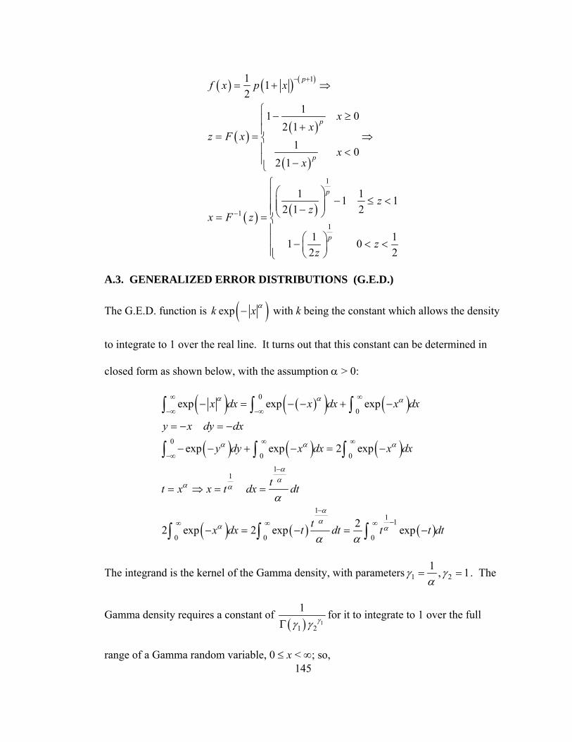
145

( ) ( ) ( )

( )( )

( )

( ) ( )

1

1

1

1

1 12

11 02 1

1 02 1

1 11 12 1 2

1 11 02 2

p

p

p

p

p

f x p x

xx

z F xx

x

zz

x F z

zz

− +

−

= + ⇒

⎧ − ≥⎪ +⎪= = ⇒⎨⎪ <⎪ −⎩

⎧⎛ ⎞⎪ − ≤ <⎜ ⎟⎪⎜ ⎟−⎪⎝ ⎠= = ⎨

⎪⎛ ⎞⎪ − < <⎜ ⎟⎪ ⎝ ⎠⎩

A.3. GENERALIZED ERROR DISTRIBUTIONS (G.E.D.)

The G.E.D. function is ( )expk x α− with k being the constant which allows the density

to integrate to 1 over the real line. It turns out that this constant can be determined in

closed form as shown below, with the assumption α > 0:

( ) ( )( ) ( )

( ) ( ) ( )

( ) ( ) ( )

0

0

0

0 0

11

11 1

0 0 0

exp exp exp

exp exp 2 exp

22 exp 2 exp exp

x dx x dx x dx

y x dy dx

y dy x dx x dx

tt x x t dx dt

tx dx t dt t t dt

α α α

α α α

αα

α α

αα

α α

α

α α

∞ ∞

−∞ −∞

∞ ∞

−∞

−

−

−∞ ∞ ∞

− = − − + −

= − = −

− − + − = −

= ⇒ = =

− = − = −

∫ ∫ ∫

∫ ∫ ∫

∫ ∫ ∫

The integrand is the kernel of the Gamma density, with parameters 1 21 , 1γ γα

= = . The

Gamma density requires a constant of ( ) 1

1 2

1γγ γΓ

for it to integrate to 1 over the full

range of a Gamma random variable, 0 ≤ x < ∞; so,

146

( )1 11

0

2 2 1exp 1t t dtα αα α α

−∞ ⎛ ⎞− = Γ ⎜ ⎟⎝ ⎠∫ . Thus, using the reciprocal of this constant, we get

the G.E.D. density of ( )exp12

x αα

α

−⎛ ⎞Γ ⎜ ⎟⎝ ⎠

. For the Gaussian distribution, α = 2 and σ2

= ½, the constant reduces to the familiar 1π

. For the double exponential, with σ = 1,

the constant is ½. Exponents (α’s) that are less than 2 produce leptokurtic densities.

Exponents greater than 2 generate platykurtic densities. In the limit as α→∞, the

G.E.D. approaches a uniform distribution over [-1,1].

Various GED densities

0

0.1

0.2

0.3

0.4

0.5

0.6

-4 -3 -2 -1 0 1 2 3 4

Value of Variable

Den

sity

a = 500a = 6a = 3a = 2a = 1.5a = 1a = .5

Figure A.1. Various GED densities. The letter “a” represents the exponent “α.”

147

We can introduce a scale factor for the G.E.D. by dividing the density and

argument of the function by some c > 0 to produce exp12

xcc

αα

α

⎛ ⎞−⎜ ⎟⎜ ⎟⎛ ⎞ ⎝ ⎠Γ ⎜ ⎟

⎝ ⎠

.

A.4. STUDENT-T DISTRIBUTIONS51

These distributions are well-known but it comes as a surprise to many that there

are two ways to generalize the distribution taught in many elementary statistics classes:

(1) a scale parameter can be introduced by dividing the density and argument by some

c > 0 just as we did above in the G.E.D., and (2) that the parameter r below which

represents the degrees of freedom can take on any non-integer positive value while the

function retains its properties as a density. Thus we have a generalized Student-t

distribution: ( )1

2 2

2

12 1 , 0, 0,

2

r

h t

rt r c t

r rcc rπ

+−⎛ ⎞⎜ ⎟ ⎛ ⎞⎝ ⎠= ⎜ ⎟⎜ ⎟⎛ ⎞ ⎝ ⎠⎜ ⎟

⎝ ⎠

+Γ+ > > − ∞ < < ∞

Γ. In

general, the kth moment of a Student-t distribution does not exist if r ≤ k. When r = 1,

we have a special case in which the Student-t distribution is the Cauchy distribution

( ) ( )211 ,h t

tt

π=

+− ∞ < < ∞ , and also is a stable distribution with α = 1.

51 Since William Sealy Gossett published under a pseudonym, “Student” is a proper noun and thus is capitalized throughout this document. Gossett worked for the Guinness Brewing Company of Dublin, Ireland. Company policy forbade its employees from publication due to a master brewer previously publishing part of a brewing process that was a Guinness company secret.

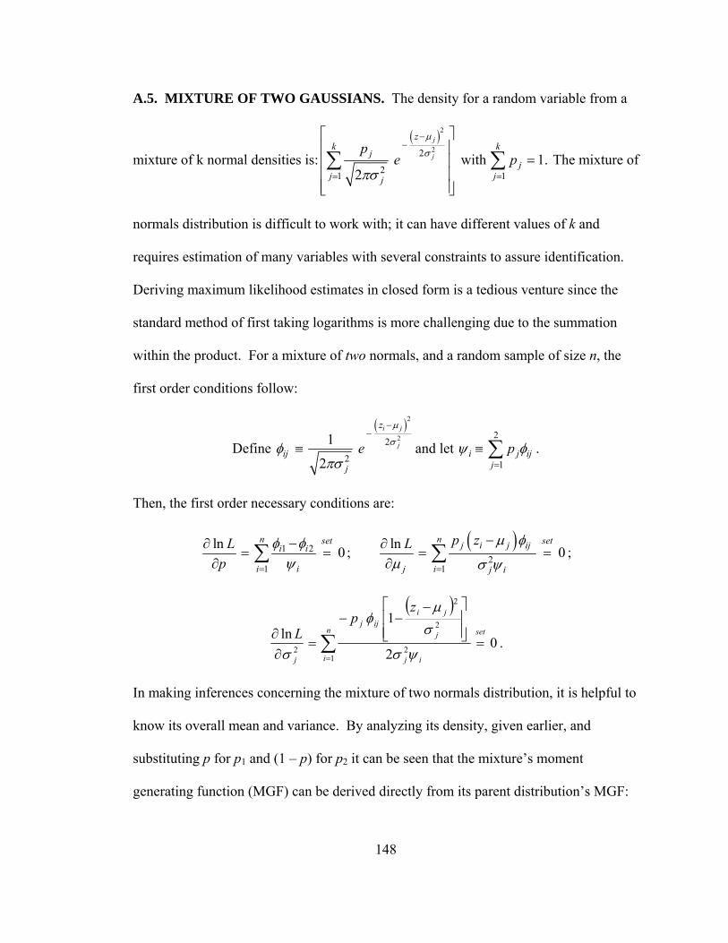
148

A.5. MIXTURE OF TWO GAUSSIANS. The density for a random variable from a

mixture of k normal densities is:

( )2

22

21 1with 1.

2

j

j

zk k

jj

j jj

pe p

μ

σ

πσ

−−

= =

⎡ ⎤⎢ ⎥

=⎢ ⎥⎢ ⎥⎢ ⎥⎣ ⎦

∑ ∑ The mixture of

normals distribution is difficult to work with; it can have different values of k and

requires estimation of many variables with several constraints to assure identification.

Deriving maximum likelihood estimates in closed form is a tedious venture since the

standard method of first taking logarithms is more challenging due to the summation

within the product. For a mixture of two normals, and a random sample of size n, the

first order conditions follow:

Define

( )2

22

2

1

2

i j

j

z

ijj

e

μ

σφπσ

−−

≡ and let 2

1i j ij

jpψ φ

=

≡ ∑ .

Then, the first order necessary conditions are:

1 2

1

ln 0n set

i i

ii

Lp

φ φψ=

−∂= =

∂ ∑ ;( )

21

ln 0n setj i j ij

j i j i

p zL μ φ

μ σ ψ=

−∂= =

∂ ∑ ;

( )

02

1ln

12

2

2

2

setn

i ij

j

jiijj

j

zp

L=

⎥⎥⎦

⎤

⎢⎢⎣

⎡ −−−

=∂∂ ∑

= ψσ

σμ

φ

σ.

In making inferences concerning the mixture of two normals distribution, it is helpful to

know its overall mean and variance. By analyzing its density, given earlier, and

substituting p for p1 and (1 – p) for p2 it can be seen that the mixture’s moment

generating function (MGF) can be derived directly from its parent distribution’s MGF:

149

( )2 21 2

1 22 2( ) 1t tt ttZE e p e p eσ σμ μ+ +

= + − .

( ) ( ) ( ) ( )( ) ( ) ( ) ( ) 211222

2111 101 μμσμσμ ppMetpetptM −+=⇒+−++= •••

( ) ( )[ ] ( ) ( ) ( )[ ] ( ) ⇒++−+++= ••• etpetptM 2222

22

2211

212 1 σμσσμσ

( ) [ ] ( )[ ]22

22

21

212 10 μσμσ +−++= ppM .

Var(Z) = M2(0) – [M1(0)]2 = pσ12 + (1-p)σ2

2 + p(1-p) (μ1 - μ2)2

The single dots in the exponential indicate the first exponent in the first line with

the parameters μ1 and σ12, while the double dots indicate the second exponent in the

first line with the parameters μ2 and σ22.

The mean is not surprising and could certainly have been inferred without

MGF’s. The determination of the variance is a little more opaque, but has the desired

result that it is positively correlated with the absolute difference in the means and gets

larger as p approaches ½.

Careful attention is required for identification of parameters. As p approaches

zero or one, either (μ1,σ12) or (μ2,σ2

2) ceases to have impact and ceases to be identified.

To help in the identification process, it is necessary to specify some set of

conditions like {p ≤ ½; if p = 0, (μ1,σ12) = (0,1); 52 if p = ½, then σ1

2 ≤ σ22; if p = ½

and σ12 = σ2

2, then μ1 < μ2}.

A symmetric mixture of two normals can result from μ1 = μ2, or from p = ½ and

σ12 = σ2

2. In this study, since we are dealing with symmetric errors, we set μ1 = μ2 = 0.

52 Since this will be a normal distribution and (μ1,σ12) will have no impact.

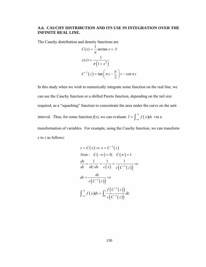
150

A.6. CAUCHY DISTRIBUTION AND ITS USE IN INTEGRATION OVER THE INFINITE REAL LINE. The Cauchy distribution and density functions are

( )( )

2

1

1( ) arctan .5

1( )1

tan cot2

C x x

c xx

C z z z

π

π

ππ π−

= +

=+

⎛ ⎞= − = −⎜ ⎟⎝ ⎠

In this study when we wish to numerically integrate some function on the real line, we

can use the Cauchy function or a shifted Pareto function, depending on the tail size

required, as a “squashing” function to concentrate the area under the curve on the unit

interval. Thus, for some function f(x), we can evaluate ( )I f x dx∞

−∞= ∫ via a

transformation of variables. For example, using the Cauchy function, we can transform

x to z as follows:

( ) ( )( ) ( )

( ) ( )( )

( )( )

( )( )( )( )( )

1

1

1

11

10

: 0; 11 1 1

z C x x C z

Note C Cdxdz dz dx c x c C z

dzdxc C z

f C zf x dx dz

c C z

−

−

−

−∞

−−∞

= ⇒ =

−∞ = ∞ =

= = = ⇒

= ⇒

=∫ ∫

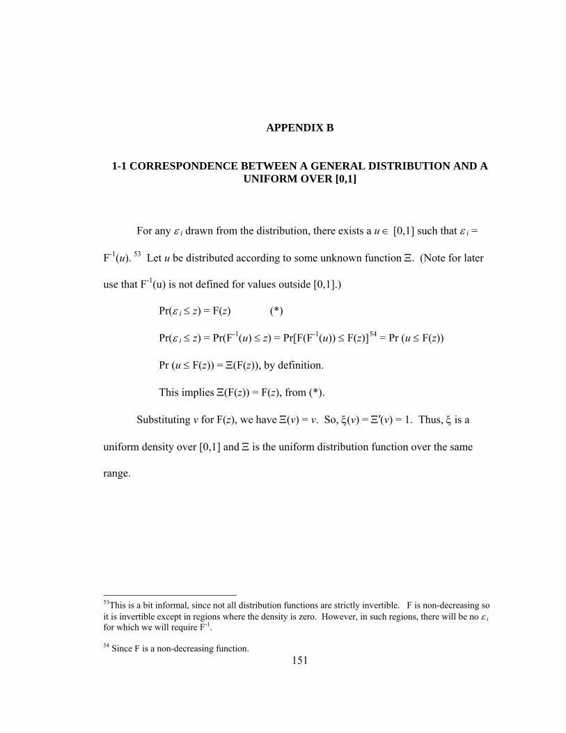
151

APPENDIX B

1-1 CORRESPONDENCE BETWEEN A GENERAL DISTRIBUTION AND A UNIFORM OVER [0,1]

For any ε i drawn from the distribution, there exists a u ∈ [0,1] such that ε i =

F-1(u). 53 Let u be distributed according to some unknown function Ξ. (Note for later

use that F-1(u) is not defined for values outside [0,1].)

Pr(ε i ≤ z) = F(z) (*)

Pr(ε i ≤ z) = Pr(F-1(u) ≤ z) = Pr[F(F-1(u)) ≤ F(z)]54 = Pr (u ≤ F(z))

Pr (u ≤ F(z)) = Ξ(F(z)), by definition.

This implies Ξ(F(z)) = F(z), from (*).

Substituting v for F(z), we have Ξ(v) = v. So, ξ(v) = Ξ′(v) = 1. Thus, ξ is a

uniform density over [0,1] and Ξ is the uniform distribution function over the same

range.

53This is a bit informal, since not all distribution functions are strictly invertible. F is non-decreasing so it is invertible except in regions where the density is zero. However, in such regions, there will be no ε i for which we will require F-1. 54 Since F is a non-decreasing function.

152

APPENDIX C

PSEUDO-RANDOM NUMBER GENERATOR AND MONTE CARLO METHODS

C.1. RANDOM NUMBER GENERATOR. For Monte Carlo simulations in this

study, the Kiss+Monster algorithm, developed by George Marsaglia in 2000, was used

exclusively. It produces random integers between 0 and 4,294,967,295 (232-1) and has

a period of 108859. It is a fast recur-with-carry generator of dimension 920. According

to Aptech, the distributors of GAUSS programming language, it seems to pass all of the

Diehard tests for random number generators for “small” samples of billions of random

numbers from its sequence. Recur-with-carry generators often have poor performance

on some of these tests, but since any practical application of using this generator will

use essentially 0% of the sequence, these problems are masked (or at least not yet found

to occur) in samples.

Recur-with-carry generators determine their next value as a function of a linear

combination of a predetermined previous number of values.

1

1int mod

k

i n iki

n i n ii

a xx a x b

b

−=

−=

⎡ ⎤⎛ ⎞⎢ ⎥⎜ ⎟⎢ ⎥⎜ ⎟= +⎢ ⎥⎜ ⎟⎢ ⎥⎜ ⎟

⎝ ⎠⎣ ⎦

∑∑

153

“Recur” refers to the dependence of a new number in the sequence on the

previous k values; “carry” relates to the second term in the brackets, the number of

times that a multiple of b would be “carried” to the next digit if we were evaluating the

sum in base b arithmetic. For the KISS + Monster, k, the dimension, is 920, though in

GAUSS, the state variable has dimension of 500.

This type of generator is to be contrasted with a linear congruent random

number generator of the form [ ]1 modn nx ax c b−= + . Linear congruent RNGs suffer

from having a period of at most b – 1 before repeating. Since the largest integer

representation is often 232 without manipulation, simple linear congruent RNGs can

generate at most 4,294,967,295 values without beginning to recycle.

It appears that KISS + Monster is more than satisfactory to avoid any repetition

for this and most other studies. To give an extreme example of how impossible it is to

describe the size of its period, imagine packing the present-day universe completely full

with super computers the size of atoms and having them generate random numbers at

incredible speeds of a trillion times a trillion numbers per second. Since there is quite a

bit of space in the universe which is not full of atoms, this means there would be many

more computers in this example than there are atoms in the universe. Ignoring the

coordination problem (and just about any other practical matter!), if these computers

had been running non-stop since the beginning of time, they would have generated

about 10152 random numbers (using the diameter of an atom as 1 Angstrom, the

diameter of the universe as 100 billion light years, the age of the universe as 13.7 billion

years, and pretending that both the atoms and the universe were spherical).

154

With the period of the Kiss+Monster random number generator being 108859, it

is fairly difficult to come up with a thought experiment that would allow one to make a

complete cycle through all of the generator's random numbers. This gives a different

meaning to the idea of infinity and, at least based on cycle length, suggests the

Kiss+Monster algorithm seems to be sufficient for random number generation.

C.2. CALCULATION OF EMPIRICAL QUANTILES

Most texts and methodologies suggest using empirical percentiles of

distributions derived by Monte Carlo simulation as estimates of theoretical

distributions. For example, if you wish to form a symmetric 90% confidence interval

from 1000 simulations, perform the repetitions, order the statistics and use the 50th

smallest statistic as the lower confidence bound. Symmetry would suggest the 50th

largest statistic x[50] as the upper confidence bound. This introduces a bit of an

inconsistency. If we wish to estimate the theoretical pth percentile, we use p/100 × S,

where S is the number of simulations. So, to approximate the theoretical 5th percentile

we find 0.05 × S, where S is the number of simulations. If we want to estimate the

theoretical 95th percentile and take 0.95 × S, we get the 51st largest order statistic x[950],

not the 50th largest x[951]. If we do use x[951], we are using 0.951 × S, which seems

inconsistent with the formula for the index of the lower confidence bound.

The problem here is using percentiles of the empirical distribution as estimators

for the percentiles of the underlying theoretical distribution. The percentile of an

empirical distribution is rarely an unbiased estimate for the percentile of theoretical

distribution. If one has a sample of 10 from a uniform distribution, u1,…, u10 and forms

order statistics, y1,…, y10, then E(y1) = 1/11, not 1/10. A direct consequence of this is

155

that if one wishes to find an unbiased estimate of the theoretical upper 5% cutoff of a

non-uniform unknown distribution with 1000 replications, one should use a weighted

average of y950 and y951. If the density is uniform in the area of this cutoff, then linear

interpolation would allow the use of .05 y950+.95 y951. Without the uniform density

presumption, it is not possible to determine whether linear interpolation is appropriate.

However, if one used 999 replications, one could confidently simply use y950 as an

unbiased estimate of the theoretical upper 5% cutoff of the non-uniform unknown

distribution, with no interpolation needed. Applications in the programs that produced

Monte Carlo simulations use a different percentile procedure than what is generally

available in GAUSS. Since the proc55 name "percentile" is already taken for the

methodology that is most often employed, the new proc that is used is immodestly

named "percyntile." Hence, percentiles used in this study are based on p% × (S+1),

rather than p% × S.

C.3. ADDITION OF 2-33 TO PSEUDO-RANDOM NUMBERS

Many random number generators have an algorithm to generate random integers

between 0 and 2k - 1, inclusively, for some integer value of k. Then, if random fractions

distributed uniformly on the unit interval are desired, the chosen random integers are

divided by 2k, which allows for random numbers between 0 and 1 – 2-k. With GAUSS

software, k = 32, so I will use that number in the foregoing.

It is a simple task to determine that the expected value of the pseudo-random

numbers generated throughout a complete cycle through the pseudo-random numbers:

k/2 × (0 + 1 – 2-k) / k = ½ - 2-(k – 1). In addition to being slightly biased, the pseudo- 55 “proc” is a term used in GAUSS for a series of statements that can be called by the main program frequently. Synonyms for this may be “macro” or “subroutine.”

156

uniform random variable has an expectation that is about 1.16415 × 10-10 too low, the

use of inverse distribution functions has trouble with zero as an argument. Since this

condition must be avoided in a program and the addition actually makes the “uniform”

numbers unbiased, it seems prudent to simply add 2-33 to each generated pseudo-random

number up front.

157

APPENDIX D

STARTING VALUES FOR ITERATIVE MAXIMUM LIKELIHOOD ESTIMATION

D.1. INITIAL ESTIMATES FOR PARAMETERS FOR USE IN MAXIMUM

LIKELIHOOD ESTIMATION. With non-Gaussian error terms, ordinary least

squares regressions are still consistent but no longer efficient methods of estimating

coefficients. So, non-standard methods can be employed under the assumption of

stable, generalized Student-t, generalized error (GED), or normal-mixture distributions.

This study focuses on the symmetric sub-class of such distributions.

With symmetric stable errors, SMSTRG, a symmetric stable regression program

(McCulloch, 1998) can be used to calculate maximum likelihood errors. For each of the

classes of errors, additional programs, similar in nature to SMSTRG, have been

developed based on the derivations shown below.

For each class of errors, initial estimates of model parameters are determined by

using trimmed least squares using the interquartile range of observations as follows.

First, residuals are determined using OLS and ordered. Then, observations with

residuals that are in the first and fourth quartiles are temporarily thrown out, and a

second set of OLS “trimmed” estimators of parameters is calculated using only the

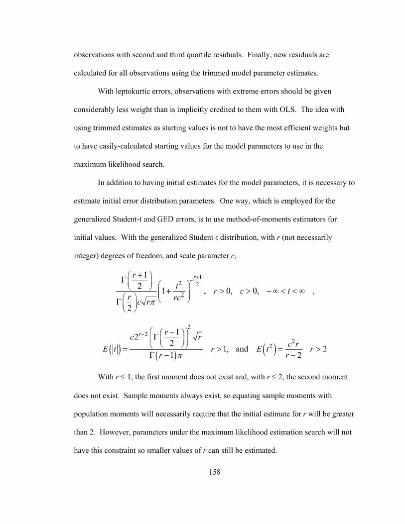
158

observations with second and third quartile residuals. Finally, new residuals are

calculated for all observations using the trimmed model parameter estimates.

With leptokurtic errors, observations with extreme errors should be given

considerably less weight than is implicitly credited to them with OLS. The idea with

using trimmed estimates as starting values is not to have the most efficient weights but

to have easily-calculated starting values for the model parameters to use in the

maximum likelihood search.

In addition to having initial estimates for the model parameters, it is necessary to

estimate initial error distribution parameters. One way, which is employed for the

generalized Student-t and GED errors, is to use method-of-moments estimators for

initial values. With the generalized Student-t distribution, with r (not necessarily

integer) degrees of freedom, and scale parameter c,

12 2

2

12 1 , 0, 0,

2

rrt r c t

r rcc rπ

+−⎛ ⎞⎜ ⎟ ⎛ ⎞⎝ ⎠ ⎜ ⎟⎜ ⎟⎛ ⎞ ⎝ ⎠⎜ ⎟

⎝ ⎠

+Γ+ > > − ∞ < < ∞

Γ ,

( ) ( ) ( )

22

22

122

1, and 21 2

r rc rc rE t r E t r

r rπ

− ⎛ ⎞⎛ ⎞⎜ ⎟⎜ ⎟

⎝ ⎠⎝ ⎠

−Γ= > = >

Γ − −

With r ≤ 1, the first moment does not exist and, with r ≤ 2, the second moment

does not exist. Sample moments always exist, so equating sample moments with

population moments will necessarily require that the initial estimate for r will be greater

than 2. However, parameters under the maximum likelihood estimation search will not

have this constraint so smaller values of r can still be estimated.

159

If sample moments are denoted as M1 and M2, we can eliminate c by equating

the sample and population ratios of the first moment with the square root of the second

moment: ( )

22

1

2

12 22

1

r r rM

rM π

− ⎛ ⎞⎛ ⎞⎜ ⎟⎜ ⎟

⎝ ⎠⎝ ⎠

−Γ −=

Γ −. This is a monotonically increasing

function of r with r > 2, illustrated below, which approaches the limit 2π

≈

0.7978845608 as r → ∞. So, there is an inverse function of the moment ratio which

will allow for an initial estimate for r. The function is relatively flat for r > 6. If the

moment ratio is by chance greater than the limiting value some high starting value such

as r̂ =100 can be chosen.

160

Initial Estimate of Degrees of Freedom

0

0.25

0.5

0.75

0 1 2 3 4 5 6 7 8 9 10 11 12 13 14 15 16 17 18 19 20

Degrees of Freedom

Rat

io o

f Mom

ents

Ratio

Asymp.

Figure D.1. Degrees of Freedom vs. Ratio of Moments in a Student-t distribution Apparent kinks in the above graph are related to the precision of the addressing of

pixels in the graphing software and not due to the function itself.

Once an estimate for r is determined, we can estimate c by equating the 2nd

population moment with the 2nd sample moment: ( )2 ˆ 2

ˆˆ

M rc

r−

= .

Some may find it improper to use a method-of-moments estimator for a

distribution which may not have moments. Although, requiring an initial starting value

for degrees of freedom greater than 2 does not prevent future maximum likelihood

iteration estimates to be greater than 2, it happened that if one started with an initial

161

estimate for degrees of freedom that is too high, the starting scale parameter was often

many orders of magnitude too high so as to compensate for the degrees of freedom

parameter.

So, alternatively, a quantile estimator can be used, following the approach of

McCulloch for stable distributions. For the Student cdf, Td(x), with d degrees of

freedom, one can calculate the function ( ))75(.)95(.

)25(.)75(.)05(.)95(.

1

1

11

11

−

−

−−

−−

=−

−=

d

d

dd

dd

TT

TTTT

df . The

ratio is invariant with respect to the scale parameter. The quantile estimator of d is

⎟⎟⎠

⎞⎜⎜⎝

⎛−−

= −

25.75.

05.95.1ˆxxxx

fd , where xp is the (100 × p) percentile of the sample distribution.

Subsequently, an estimate for the scale parameter can be determined from a function of

d̂ : ( )

.75 .25ˆˆ

x xcg d

−= with ( ) )75(.2)25(.)75(. 111 −−− =−= ddd TTTdg .

The recommendation adopted for this study was to use the quantile estimator

whenever the moment estimator suggested degrees of freedom under 3. Some limited

simulation studies show that the moment estimator has a lower mean squared error for

degrees of freedom higher than 3, but much higher for degrees of freedom less than 3.

An alternate methodology which has not been explored is to recognize that the method-

of-moments estimators are biased and to map the moment estimator to a different scale

based on sample size; for example, if the scale suggested 2.1 degrees of freedom with

100 observations, one might reasonably conclude that the starting degrees of freedom

could be some lower number like 1. However, it is important to remember to keep this

methodology as simple as possible, since these are only starting values and that more

162

efficient parameter estimates will be obtained through the subsequent maximum

likelihood estimation.

Using a similar approach, GED errors are distributed according to:

exp , 0, 0,12

x c xcc

αα α

α

⎛ ⎞⎜ ⎟⎜ ⎟⎛ ⎞ ⎝ ⎠⎜ ⎟

⎝ ⎠

− > > − ∞ < < ∞Γ

Then, ( ) ( )2

2

2 3

and1 1

c cE x E xα α

α α

⎛ ⎞ ⎛ ⎞⎜ ⎟ ⎜ ⎟⎝ ⎠ ⎝ ⎠⎛ ⎞ ⎛ ⎞⎜ ⎟ ⎜ ⎟⎝ ⎠ ⎝ ⎠

Γ Γ= =

Γ Γ. Employing the same equating of

sample and population ratios as with the Student-t problem, we again eliminate c:

1

2

2

3 1MM

α

α α

⎛ ⎞⎜ ⎟⎝ ⎠

⎛ ⎞ ⎛ ⎞⎜ ⎟ ⎜ ⎟⎝ ⎠ ⎝ ⎠

Γ=

Γ Γ, which is a monotonic function increasing in α, illustrated

below, which approaches the limit 32

≈ 0.8660254038 as α → ∞. So, there is an

inverse function of the moment ratio which will allow for an initial estimate for α. The

function is relatively flat for α > 6. If the moment ratio is by chance greater than the

limiting value some high starting value such as α̂ =20 can be chosen:

163

Initial Estimate of Alpha

0

0.25

0.5

0.75

0 1 2 3 4 5 6 7 8 9 10 11 12 13 14 15 16 17 18 19 20

Alpha

Rat

io o

f Mom

ents

Ratio

Asymp.

Figure D.2. Power vs. Ratio of Moments in a GED distribution

We can then use one of the two moment equations to estimate c; e.g., 1

1ˆˆ2ˆ

c M α

α

⎛ ⎞⎜ ⎟⎝ ⎠⎛ ⎞⎜ ⎟⎝ ⎠

Γ=

Γ.

With a mixture of two normals, there are three parameters to be estimated rather

than two; consequently, three sample moments are necessary. It would seem that using

a method similar to that developed for the other error distributions would be quite a bit

more complicated. Amazingly, after some not-too-apparent algebraic manipulation,

there is actually a closed-form solution which does not even require any exotic

functional estimation!

The error distribution is according to:

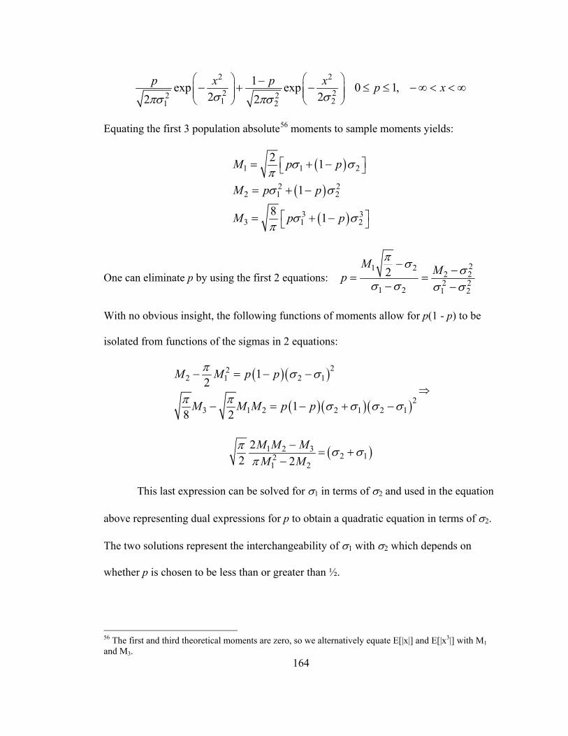
164

2 2

2 22 21 21 2

1exp exp 0 1,2 22 2

p x p x p xσ σπσ πσ

⎛ ⎞ ⎛ ⎞⎜ ⎟ ⎜ ⎟⎜ ⎟ ⎜ ⎟⎝ ⎠ ⎝ ⎠

−− + − ≤ ≤ − ∞ < < ∞

Equating the first 3 population absolute56 moments to sample moments yields:

( )

( )

( )

1 1 2

2 22 1 2

3 33 1 2

2 1

1

8 1

M p p

M p p

M p p

σ σπσ σ

σ σπ

⎡ ⎤⎣ ⎦

⎡ ⎤⎣ ⎦

= + −

= + −

= + −

One can eliminate p by using the first 2 equations: 21 2

2 22 2

1 2 1 2

2M Mp

π σ σσ σ σ σ

− −= =− −

With no obvious insight, the following functions of moments allow for p(1 - p) to be

isolated from functions of the sigmas in 2 equations:

( ) ( )

( ) ( ) ( )

222 1 2 1

23 1 2 2 1 2 1

12

18 2

M M p p

M M M p p

π σ σ

π π σ σ σ σ

− = − −

− = − + −⇒

( )1 2 32 12

1 2

22 2

M M MM M

π σ σπ

− = +−

This last expression can be solved for σ1 in terms of σ2 and used in the equation

above representing dual expressions for p to obtain a quadratic equation in terms of σ2.

The two solutions represent the interchangeability of σ1 with σ2 which depends on

whether p is chosen to be less than or greater than ½.

56 The first and third theoretical moments are zero, so we alternatively equate E[|x|] and E[|x3|] with M1 and M3.

165

Explicit estimates for the parameters follow (if 1 2ˆ ˆσ σ≠ ):

( ) ( ) ( ) ( )2 2 21 2 3 1 2 3 2 1 3 1 2

2 21 2

1 2 31 22

1 2

1 2

1 2

2 2 2 4 22 2ˆ

2 42ˆ ˆ

2 2

ˆ2ˆ

ˆ ˆ

M M M M M M M M M M M

M MM M MM M

Mp

π π π πσ

ππσ σ

ππ σ

σ σ

− ± − − − −=

−

−= −−

−=

−

The knife-edge case ( 1 2ˆ ˆσ σ= ) is a case equivalent to a Gaussian distribution (a

single normal distribution rather than a mixture of two) and can be thought of either

as p̂ being indeterminate between 0 and 1, exclusively, or p̂ being 1, 1σ̂ being

estimated by 2M and 2σ̂ being indeterminately nonnegative (or p̂ being 0, 2σ̂ being

estimated by 2M and 1σ̂ being indeterminately nonnegative).57

If the equations above do not yield legitimate values for the parameters, I would

choose starting values as follows:

2 21 2

31ˆ ˆ ˆ, ,2 2 2

M Mp σ σ= = =

57 To identify the estimate, one can impose the requirement that one of the following three sets of conditions hold: (1) 1 2ˆ ˆσ σ< , (2) 1 2ˆ 1, ˆ ˆ1, 1p σ σ= < = , or (3) 1 2ˆ 0, ˆ ˆ1, 1p σ σ= = > .

166

APPENDIX E

INVARIANCE OF LM STATISTIC WITH RESPECT TO LINEAR TRANSFORMATIONS OR EXPONENTIATION

The Lagrange multiplier statistic is invariant with respect to a linear change of

basis functions. In addition, the statistic is also invariant with respect to an

exponentiation of the basis functions.

First consider the ordinary alternative hypothesis:

( ) ( ) ( ) ( )1

01

1 1 , 0m

j j jj

g z z z z dzφ α φ α φ φ=

′= + = + =∑ ∫ ,

where the non-indexed α and φ are vectors. ( )zφ is a basis that spans a space of smooth

functions. We will restrict ourselves to a basis with orthonormal functions. Forα ∈ Α ,

where A is a convex subspace of ℜm that includes the origin as an interior point, we

have ( ) 0,g z zφ ≥ ∀ . So ( )g zφ is a density whenα ∈ Α .

The likelihood function of interest is:

Lφ(α;x) = 1

( ; )n

ii

g xφ α=

∏ ⇒ Λφ (α;x) = ( )1

log ;n

ii

g xφ α=∑ = ( )

1 1log 1

n m

j j ii j

xα φ= =

⎛ ⎞+⎜ ⎟⎜ ⎟

⎝ ⎠∑ ∑ ,

where Λφ is the logarithm of the likelihood function. The jth first derivative, evaluated

at α = 0, is:

167

( )

( )( )

1 10

1 0

log

1

n nj i

j imj i i

k k ik

xLx

x

φ

α

α

φφ

αα φ= ==

= =

∂= =

∂+

∑ ∑∑

,

so the transpose of the “score” vector of first derivatives, evaluated at α = 0, for the LM

Statistic is:

( ) ( ) ( )11 1

0 , ,n n

i m ii i

s x xφ φ φ= =

⎛ ⎞′ = ⎜ ⎟

⎝ ⎠∑ ∑K

A typical element of the Hessian matrix is:

( ) ( )

( )

2

21

11

n j i j i

mij jk k i

k

x x

x

φ φ φα α

α φ

′

=′

=

−∂ Λ

∂ ∂ ⎡ ⎤⎢ ⎥⎣ ⎦

= ∑+∑

,

so a typical element of the Fisher information matrix, evaluated at the null hypothesis,

for the LM statistic is:

( ) ( ) ( )

( )( ) ( )

2

, 0 0 021 1

1

log0

1

n nj i j i

j j j i j imj j i i

k k ik

x xLI E E E x x

x

φφ α α α

φ φφ φ

α αα φ

′′ ′= = =

′ = =

=

⎧ ⎫⎪ ⎪

⎛ ⎞ −∂ ⎡ ⎤⎪ ⎪= − = − =⎜ ⎟ ⎨ ⎬ ⎢ ⎥⎜ ⎟∂ ∂ ⎡ ⎤ ⎣ ⎦⎪ ⎪⎝ ⎠ +⎢ ⎥⎪ ⎪

⎣ ⎦⎩ ⎭

∑ ∑∑

= ( ) ( ) ( ) ( ) ( ) ( ) ( )1 1

0 00 01 1

;n n

j i j i j i j i i i j ji i

E x x x x g x dx n z z dzα αφ φ φ φ α φ φ′ ′ ′= =

= =

⎡ ⎤ = =⎣ ⎦∑ ∑∫ ∫

The Lagrange multiplier statistic is LMφ = sφ′(0)Iφ (0)-1sφ (0). Since ( )zφ is

orthonormal, I is the identity matrix multiplied by the scalar n; so, the LM statistic

reduces to 1/n sφ′(0)sφ (0).

168

Selecting an alternative basis, ( ) ( )* z M zφ φ= where M is nonsingular and

deterministic, we get ( ) ( )** *

11 1

, ,n n

i m ii i

s x xφ φ φ= =

⎛ ⎞′ = ⎜ ⎟

⎝ ⎠∑ ∑K or *s Msφφ = .

The information matrix with respect to the alternative basis:

( ) ( )

( ) ( )

*

*

1 * *0

1

01 1 1 1

I n z z dz

n M z z M dz MI M

I M I M

φ

φ

φφ

φ φ

φ φ− − − −

′=

′ ′ ′= =

′=

∫

∫

The Lagrange multiplier statistic with respect to the alternative basis is

( ) ( ) ( )* * * *1 1 1 1 1LM LMs I s s M M I M Ms s I sφ φ φ φ φ φ φφ φ φ φ

− − − − −′ ′ ′ ′ ′= = = =

Now, let us turn our attention to an exponentiated form for our alternative

density:

( )( )

( )

( )

( )

1

1 1 10 0

g z z

e g z z

e eg ze dz e dz

φ

φ

α φ

α φ

′+

′+= =

∫ ∫

The denominator is a constant necessary for the density to integrate to unity, which we

can call Cφ (α). The attractiveness of this choice of function is that ge is a density for all

α ∈ ℜm, rather than just a subset of ℜm.

The likelihood function of interest is:

Le(α;x) = 1

( ; )n

e ii

g x α=

∏ ⇒ Λe (α;x) =

( )1

log ;n

e ii

g x α=∑ = ( ) ( )

1 11 log

n m

j j ii j

x n Cα φ α= =

⎛ ⎞+ −⎜ ⎟⎜ ⎟

⎝ ⎠∑ ∑ ,

Thus, a typical element of the score is:

169

( ) ( ) ( )( )

( )

( )

1

1

11

0

11 1 1 1

0

1 log

m

j jj

m

j jj

zn m n j

j j i j izj i j i

z e dzx n C x n

e dz

α φ

α φ

φα φ α φ

α

=

=

+

+= = =

∑⎡ ⎤⎛ ⎞∂

+ − = −⎢ ⎥⎜ ⎟⎜ ⎟∂ ⎢ ⎥ ∑⎝ ⎠⎣ ⎦

∫∑ ∑ ∑∫

Evaluated at α = 0, this becomes:

( )( )

( )1

0

1 1

n njj i j i

i i

e z dzx n x

e

φφ φ

= =

− =∫∑ ∑ ,

since the integral of each basis function over the unit interval is zero. A typical element

of the Hessian is:

( ) ( ) ( )( )

( )

( )

1

1

11

0

11 1 1 1

0

1 log

m

j jj

m

j jj

zn m n j

j j i j izj j ji j i

z e dzx n C x n

e dz

α φ

α φ

φα φ α φ

α α α

=

=

+

+′ ′= = =

⎡ ⎤∑⎢ ⎥⎡ ⎤⎛ ⎞∂ ∂ ⎢ ⎥+ − = −⎢ ⎥⎜ ⎟ ⎢ ⎥⎜ ⎟∂ ∂ ∂⎢ ⎥ ∑⎝ ⎠⎣ ⎦ ⎢ ⎥⎢ ⎥⎣ ⎦

∫∑ ∑ ∑∫

( ) ( ) ( )( )

( )( )

( )( )

( )

1 1 11 1 11 1 1

0 0 0

2

m m m

j j j j j jj j j

z z z

j j j jC z z e dz z e dz z e dz

nC

α φ α φ α φ

α φ φ φ φ

α

= = =+ + +

′ ′

⎡ ⎤⎛ ⎞ ⎛ ⎞∑ ∑ ∑⎢ ⎥⎜ ⎟ ⎜ ⎟−⎢ ⎥⎜ ⎟ ⎜ ⎟⎜ ⎟ ⎜ ⎟⎢ ⎥⎝ ⎠ ⎝ ⎠= − ⎢ ⎥⎡ ⎤⎢ ⎥⎣ ⎦

⎢ ⎥⎢ ⎥⎣ ⎦

∫ ∫ ∫

The information matrix is the expected value of the Hessian. Here we evaluate the

Information matrix at α = 0.

( ) ( )1

11

, 0 0

0

;

m

j jj

e jjeI H z dzC

α φ

α

α

αα

=+

′ =

=

⎡ ⎤∑⎢ ⎥⎢ ⎥⎡ ⎤ = −⎣ ⎦ ⎢ ⎥⎢ ⎥⎣ ⎦

∫

170

( ) ( ) ( )( ) ( )( )( ) ( )

1 1 12 210 0 0

2 0

j j j j

j j

e z z dz e z dz z dzn n z z dz

e

φ φ φ φφ φ

′ ′

′

⎡ ⎤−⎢ ⎥= =⎢ ⎥

⎢ ⎥⎣ ⎦

∫ ∫ ∫∫

So, the information and score evaluated at the null hypothesis and, hence, also the

Lagrange multiplier statistic, are equivalent whether or not the basis is exponentiated.

LMe = LMφ

This suggests that the convex subset of ℜm on which the vector α and a regular

basis forms legitimate densities is an isomorphism of the entire space ℜm, the set on

which α and an exponentiated basis forms densities. In this isomorphism, α = 0, which

is an interior point for regular bases corresponds to α = 0, the center of ℜm, for

exponentiated bases. Thus, in one sense, the null hypothesis can be thought to be in a

“central region” of the space of alternative hypotheses, with alternatives available in

any direction.

171

APPENDIX F

UNCONDITIONAL CALCULATION OF σ2

Rather than use pseudo-random numbers for Monte Carlo simulation, for some

purposes it is better to use a different scheme of deterministic numbers to draw from the

joint distribution of p-tuples of σ2’s. So-called quasi-random numbers are better suited

for the purpose of estimating σ1 in Chapter 8, because they are ex-post more equally

distributed throughout the domain over which we will be integrating. Because of that,

an average of the summation of n properly-chosen evaluations of a function will

converge to the expected value of the function asymptotically at a quicker rate than

Monte Carlo simulation.58

F.1. QUASI-RANDOM NUMBERS

Figure F.1 shows comparisons of quasi-random numbers with pseudo-random

numbers. Each set has 150 members. The pseudo-random numbers were generated by

Excel’s random number generator, whereas the quasi-random numbers are functions 58 In some literature, Monte Carlo methods of multi-dimensional integration are claimed to have convergence rates that are superior to deterministic methods by appealing to stochastic properties and independence of successive draws. One actually can verify empirically that Monte Carlo methods often work better than some deterministic methods. However, when one realizes that Monte Carlo methods that use computer algorithms as random number generators are themselves actually deterministic rather than truly random, one must reason that something besides randomness is causing the improved convergence rates. Since a string of Monte Carlo random numbers are not independent, many laws of large numbers or central limit theorems that are appealed to do not strictly apply to these sequences. Thus, if pseudo-random numbers help to produce improved convergence rates, it is reasonable to widen our search to other deterministic methodologies.

172

that fill in a unit square59 evenly by “remembering” where it has and has not already

been (the functions could also be used to populate a d-dimensional unit hyper-interval

though I would have a difficult time showing examples in a dissertation that is on a

collection of essentially 2-dimensional planes). All the examples of quasi-random

number sequences, which are not random at all, take advantage of the infinite non-

repeating representation of the fractional parts of irrational numbers.

59 The functions could also be used to populate a d-dimensional unit hyper-interval though I would have a difficult time showing examples in a dissertation that is on a collection of essentially 2-dimensional planes!

173

Sample A

0

0.1

0.2

0.3

0.4

0.5

0.6

0.7

0.8

0.9

1

0 0.1 0.2 0.3 0.4 0.5 0.6 0.7 0.8 0.9 1

Sample B

0

0.1

0.2

0.3

0.4

0.5

0.6

0.7

0.8

0.9

1

0 0.1 0.2 0.3 0.4 0.5 0.6 0.7 0.8 0.9 1

Sample C

0

0.1

0.2

0.3

0.4

0.5

0.6

0.7

0.8

0.9

1

0 0.1 0.2 0.3 0.4 0.5 0.6 0.7 0.8 0.9 1

Sample D

0

0.1

0.2

0.3

0.4

0.5

0.6

0.7

0.8

0.9

1

0 0.1 0.2 0.3 0.4 0.5 0.6 0.7 0.8 0.9 1

Sample E

0

0.1

0.2

0.3

0.4

0.5

0.6

0.7

0.8

0.9

1

0 0.1 0.2 0.3 0.4 0.5 0.6 0.7 0.8 0.9 1

Sample F

0

0.1

0.2

0.3

0.4

0.5

0.6

0.7

0.8

0.9

1

0 0.1 0.2 0.3 0.4 0.5 0.6 0.7 0.8 0.9 1

Sample G

0

0.1

0.2

0.3

0.4

0.5

0.6

0.7

0.8

0.9

1

0 0.1 0.2 0.3 0.4 0.5 0.6 0.7 0.8 0.9 1

Sample H

0

0.1

0.2

0.3

0.4

0.5

0.6

0.7

0.8

0.9

1

0 0.1 0.2 0.3 0.4 0.5 0.6 0.7 0.8 0.9 1

Figure F.1. Examples of quasi-random numbers and pseudo-random numbers over the unit square.

It is easy to see that Samples B, E, and H have a more deterministic pattern and

are thus different than typical pseudo-random numbers. These come from quasi-

random number formulae. As it turns out, Sample C is also quasi-random, but perhaps

174

has less desirable properties for integrating over the unit square. Samples A, D, F, and

G are sets of Excel pseudo-random numbers.

We define the function {kα} to be the fractional part of the number kα, or in

other words the part of the decimal expansion of kα that follows the decimal point,

including the decimal point. Then we can define the sets of numbers illustrated in

Figure F.1 to be, in (x,y) coordinates (in all cases, k = 1, 2, …, 150):

Sample B: { } { }( )5,3 kk Weyl sequence

Sample C: ( ){ } ( ){ }( )7,3 21

21 ++ kkkk Haber sequence

Sample E: { } { }( )3 23 2,2 kk Niederreiter sequence

Sample F: { } { }( )7/511/3 , keke Baker sequence

To generalize these to multiple dimensions: with Weyl, all the terms are

{kpi1/2}, where the pi, are distinct prime numbers; with Haber, again all the terms have

factors which are distinct prime numbers; with Niederreiter, the general term is

{k2j/d+1}, where j = 1, 2, …, d and d is the number of dimensions; in the Baker

sequence, the exponents of e are distinct rational numbers.

In Numerical Methods in Economics (1998), Judd states that these methods

“have not been extensively used in economic analysis or econometrics. They have,

however, received substantial attention in the financial literature, even the financial

press …”

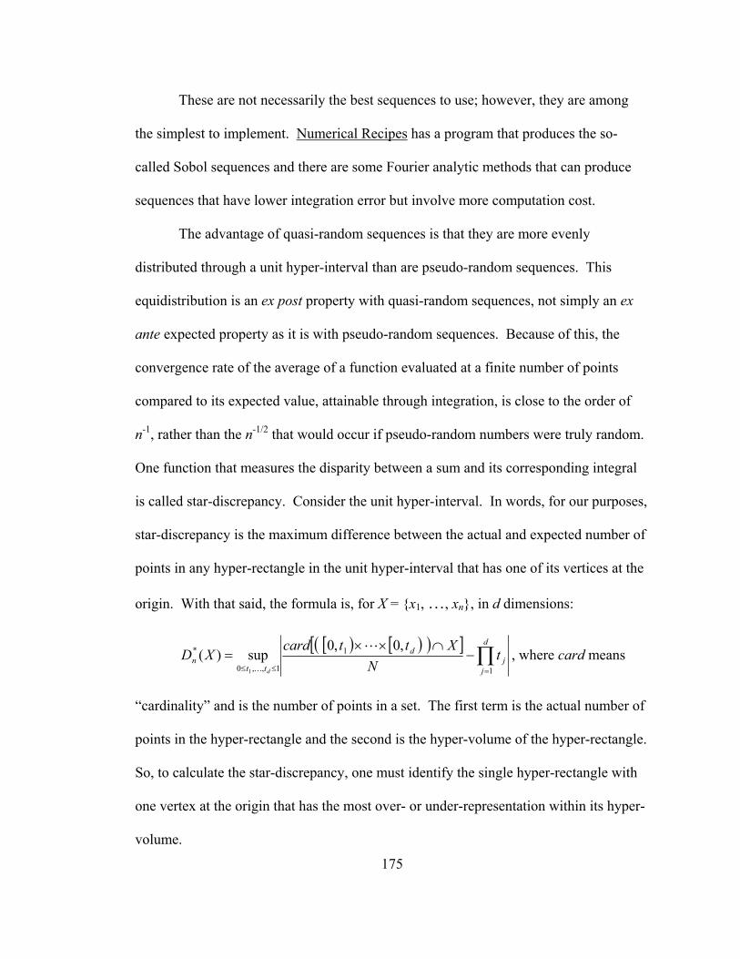
175

These are not necessarily the best sequences to use; however, they are among

the simplest to implement. Numerical Recipes has a program that produces the so-

called Sobol sequences and there are some Fourier analytic methods that can produce

sequences that have lower integration error but involve more computation cost.

The advantage of quasi-random sequences is that they are more evenly

distributed through a unit hyper-interval than are pseudo-random sequences. This

equidistribution is an ex post property with quasi-random sequences, not simply an ex

ante expected property as it is with pseudo-random sequences. Because of this, the

convergence rate of the average of a function evaluated at a finite number of points

compared to its expected value, attainable through integration, is close to the order of

n-1, rather than the n-1/2 that would occur if pseudo-random numbers were truly random.

One function that measures the disparity between a sum and its corresponding integral

is called star-discrepancy. Consider the unit hyper-interval. In words, for our purposes,

star-discrepancy is the maximum difference between the actual and expected number of

points in any hyper-rectangle in the unit hyper-interval that has one of its vertices at the

origin. With that said, the formula is, for X = {x1, …, xn}, in d dimensions:

[ ) [ )( )[ ] ∏

=≤≤−

∩××=

d

jj

d

ttn t

NXttcard

XDd 1

1

1,,0

* ,0,0sup)(1

L

K

, where card means

“cardinality” and is the number of points in a set. The first term is the actual number of

points in the hyper-rectangle and the second is the hyper-volume of the hyper-rectangle.

So, to calculate the star-discrepancy, one must identify the single hyper-rectangle with

one vertex at the origin that has the most over- or under-representation within its hyper-

volume.

176

In the examples pictured earlier, the star discrepancies, calculated by a GAUSS

program60, are:

Pseudo-sequences Quasi-sequences

Sample A: 0.079568 Sample B: 0.026347

Sample D: 0.133363 Sample C: 0.117259

Sample F: 0.116767 Sample E: 0.033468

Sample G: 0.088959 Sample H: 0.049044

So, your eyes did not lie to you. Even though Sample C is quasi-random, its

coverage is less uniform ex post than the other quasi-random sequences, at least with

150 points.

So, how can we practically use one of these or another quasi-random sequence

in our problem?

In two dimensions, we need to transform the domain to the unit square, which

could be done via estimated distribution functions. The first one of these could be an

initial estimate of the unconditional distribution of σ2 with the second being an estimate

of the conditional distribution of σ2t | σ2

t-1. With more than 2 dimensions, we would

also need the conditional distributions of σ2t | σ2

t-1, σ2t-2, etc.

60 The program runs through (n+1) × (n+1) rectangles, with the vertex diagonal from the origin being defined by the cross product of the x-coordinates of the n points (plus the value “1”) with the y-coordinates of the n points (plus the value “1”). For each of these rectangles, it determines the proportion of points in the interior of the rectangle and also the proportion of points in the interior of an “outer rectangle”, which is calculated by multiplying the coordinates by 1 + machine epsilon or 1+ 2.220446049250313 × 10-16. Then a comparison is made between the proportions and the area of the rectangle. The absolute difference that is the largest of all those 2 × (n+1) × (n+1) comparisons is the star discrepancy. (If by chance, any x- or y-coordinates are zero, they will be counted in the proportion.)

177

For completeness, the quasi-random sequence that minimizes star-discrepancy

in one dimension, is simply {k/(n+1)}, k = 1, 2, …, n, which is the sequence which is

often the procedure used in the event of iteration being necessary in one dimension.

F.2. RULE OF THUMB FOR MAXIMAL “REASONABLE” VALUES OF σ2

Of course, the support of σ2 runs to +∞. However, if you want to have some

idea what large reasonable values are so you know over what interval you may need to

numerically compute the unconditional density in Chapter 8, first pick a small

probability, say, p = 10-6. Following, I will show an example of how to pick a number

that is on the order of the inverse distribution function at p. For my example, I will use

Gaussian errors with a GARCH(1,1) model. I will use the same notation as in the

footnote on the first page: σ2t = ω + ξ1η2

t - 1 + ζ1 σ2t – 1.

With Gaussian errors, we can use the χ2(1) function; with other errors, we will

have to use the square of the error function. In this case anyway, we know that

[χ2(1)]-1(1 – p) = [Φ-1(1 – p/2)]2.

Consider the one-in-a-million situation we are interested in. A 0.000001 event

could happen in many ways, but since we are looking for an estimate rather than an

exact value, let us consider two. For both of these let us assume that we are at a state

with the mean level of σ2; although, the values will not be much different if we are a bit

larger or smaller than the average. Now, we could get that 0.000001 event right away.

Or, it could happen that we get 2 consecutive one-in-a-thousand draws.

The first circumstance will result in the next variance being calculated as:

178

( ) ( )[ ] ( )( )11

1

1111

122

1193.231

11,1

ξζξω

ξζωζξχωσ

−−−+

=−−

+−+=− p

The second example will result in a variance being calculated, in two steps:

( ) ( )[ ] ( )( )

( ) ( )[ ] ( )( )

( ) ( )( )11

111

11

111

122

11

1

1111

122

1183.10183.10

1183.101

1,1)2(

1183.101

11,1)1(

ξζξζξω

ξζξω

ζξχωσ

ξζξω

ξζωζξχωσ

−−−++

=−−

−++−+=

−−−+

=−−

+−+=

−

−

p

pinitial

Depending on the values of the parameters, either one of these final values could be

higher than the other. I would conjecture that there is a good chance that the maximum

of the two will be higher than the cutoff value sought and certainly be near to the order

of the value at the cutoff probability, p.

179

APPENDIX G

ROUNDING CONCERNS

G.1. ROUNDING ERRORS IN POLYNOMIALS

There are two types of error of concern in the evaluation of polynomials. This

first is an error in the representation of the coefficients of the polynomial. If the

polynomial is truly p(x), let us call the computational representation of the polynomial

p*(x). If the coefficients of p*(x) are near but not exactly equal to the coefficients of

p(x), there would be coefficient representation error, even if there were no further

rounding error in evaluating the polynomial at a particular value of x. For many

polynomials, the coefficient representation error is large and pervasive for relatively

large values of x above 0.9. Additionally, unlike some other types of rounding errors,

this error is large and in the same direction for all relatively large values of x.

The polynomial evaluation error, the rounding error that occurs in the

evaluation of p(x), where p(x) = p*(x) exactly with no coefficient representation error

will also have an effect. While this error is more random, since we are interested in

calculating critical values, one can expect that these too will have some undesirable

effect on the calculation of simulated critical values.

180

For any polynomial in x, one can imagine an error function as a function of x,

based on the rounding that occurs at each calculation. This function will be somewhat

periodic if one assumes that x itself also contributes to the error. For example, if x can

only be represented to 13 hexadecimal digits, there will be a tiny period of 16-13 where

the error introduced by x peaks and falls.

However, there is a more significant event happening in the calculation of the

Neyman basis. It was assumed that one could calculate as many basis functions as one

would like; however, since the number of digits in some of the coefficients grow rather

quickly while other coefficients remain equal to 1, we will see some significant

calculation errors when we go about using the polynomials in rounded form unless all

the coefficients are such that they can be represented in 16-digit hexadecimal form.

The recursion formula is ( ) ( ) ( ) ( ) ( )11

2 1 2 11n n

nn y f y nf y

f yn

−+

+ − −=

+with

f0(y) = 1 and f1(y) = 2y – 1.

As it turns out many of the coefficients that have only 17-digits can actually be

represented with zero rounding error. This is not immediately clear from the recursion

formula but a look at the coefficients shows that they are evenly divisible by several

numbers. If some of these numbers are powers of two, exact representation is possible

even with a large degree of digits. In base 10, 1,000,000 can be represented exactly

with two significant digits but 301 cannot.

However, if we look at the 25th basis function, we will see that it contains,

among others, the following terms:

181

-34117964696719800 y22 + 87835611240491400y21-168415237204594380 y20

+249504055117917600y19-292438194472624200 y18+275435973863750700y17-

210584646684190350 y16+131486998905250560y15-67237669894730400 y14

All these terms have from 17 to 18 digits and not all of them can be represented

with no rounding error in double precision hexadecimal floating point notation.

The actual representation of the coefficients is:

-34117964696719799 y22 + 87835611240491396y21-168415237204594380 y20

+249504055117917600y19-292438194472624192 y18+275435973863750719y17-

210584646684190350 y16+131486998905250560y15-67237669894730398 y14

This leaves a systematic difference of: y22 - 4y21 + 8y18 + 19y17+ 2y14.

This function takes on a maximum value of 26 at one and is pictured on the next

page. In the calculation of the LM statistic, this systematic error function will hit an

element of the inverse of the Fisher information matrix which equals 2m + 1, or, in this

case, 51, before again being multiplied by the error function.

What is worse is that the calculation of the 26th basis function is based on the

rounded coefficients of the 25th, so the errors will multiply quite quickly.

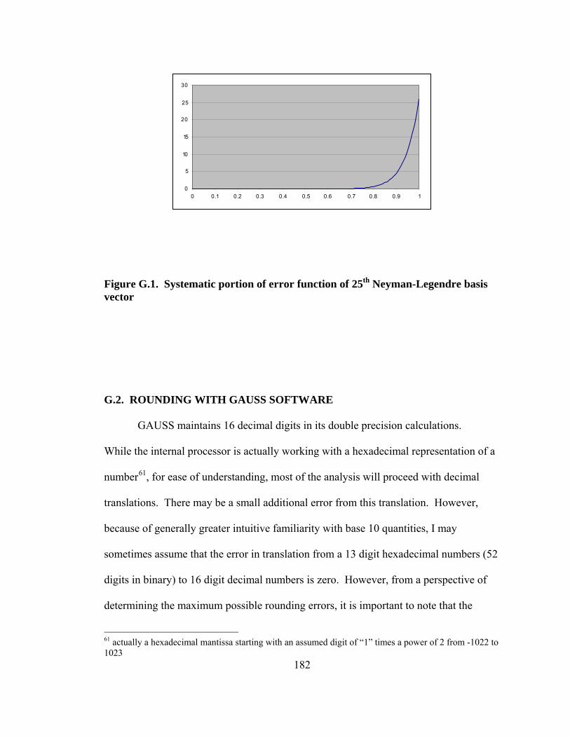
182

0

5

10

15

20

25

30

0 0.1 0.2 0.3 0.4 0.5 0.6 0.7 0.8 0.9 1

Figure G.1. Systematic portion of error function of 25th Neyman-Legendre basis vector

G.2. ROUNDING WITH GAUSS SOFTWARE

GAUSS maintains 16 decimal digits in its double precision calculations.

While the internal processor is actually working with a hexadecimal representation of a

number61, for ease of understanding, most of the analysis will proceed with decimal

translations. There may be a small additional error from this translation. However,

because of generally greater intuitive familiarity with base 10 quantities, I may

sometimes assume that the error in translation from a 13 digit hexadecimal numbers (52

digits in binary) to 16 digit decimal numbers is zero. However, from a perspective of

determining the maximum possible rounding errors, it is important to note that the

61 actually a hexadecimal mantissa starting with an assumed digit of “1” times a power of 2 from -1022 to 1023

183

errors described in base 10 are actually a bit smaller than the actual maximum possible

rounding errors.

To illustrate the translation problem, consider the binary representation of 253.

GAUSS calculates this number with zero rounding error to be 9007199254740992 in

base 10. But, observation of the following series of additions shows that only 13

hexadecimal digits are being used:

253 = 9007199254740992. 253 + 1 = 9007199254740992. 253 + 2 = 9007199254740994. 253 + 3 = 9007199254740996. 253 + 4 = 9007199254740996. 253 + 5 = 9007199254740996. 253 + 6 = 9007199254740998. 253 + 7 = 9007199254741000. 253 + 8 = 9007199254741000. 253 + 9 = 9007199254741000. 253 + 10 = 9007199254741002. 253 + 11 = 9007199254741004. 253 + 12 = 9007199254741004. 253 + 13 = 9007199254741004. 253 + 14 = 9007199254741006. 253 + 15 = 9007199254741008. 253 + 16 = 9007199254741008. 253 + 17 = 9007199254741008. 253 + 18 = 9007199254741010.

The fact that all the sums are even numbers gives a clue that the units digit is not

being used. The hexadecimal representations of 1 to 18 (01 to 12) are all being rounded

so that the units digit is zero prior to addition. Of less important note, the rounding also

occurs in a non-traditional way. Instead of always rounding “up” or “down,” whenever

rounding is necessary, the results are being rounded “even.” In base 10, rounding even

would round 0.75 to 0.8, while rounding 0.25 to 0.2. As a general rule, this means that

the least significant digit in the rounded answer is even. With a binary representation,

184

“rounding even” amounts to always finding the closest representation such that the least

significant digit is zero, since the only even digit in base 2 is zero, or rounding to the

nearest multiple of four. In hexadecimal, rounding even means rounding the least

significant digit to 2, 4, 6, 8, A, C, or E.

The number 253 (a one followed by 53 zeros in binary, a two followed by 13

zeros in hexadecimal) can be represented exactly correctly in hexadecimal floating

point with only 13 hexadecimal digits in the mantissa since it can be represented as a 1,

which is always assumed, followed by 13 hexadecimal digits (after the “decimal” point)

times 2 raised to the 53rd power (using an exponent of 53). An exponent of 53 signifies

that the mantissa is to be multiplied by 253.

However, the number 253+1 cannot be represented exactly correctly as a 13-digit

hexadecimal floating point number; it would be 1.00000000000008 × 253. Focusing on

the last digit, we see that this represents 8 × 16-14 × 253 = 1. However, the last digit, “8,”

is in the 14th place so it must be dropped. The choices are for 253+1 to be represented

either as 1.0000000000000 × 253 or 1.0000000000001 × 253, so the answer can be

represented as 253 plus either 0 × 16-13 × 253 = 0 or 1 × 16-13 × 253 = 2.

Note that there is no corresponding problem with subtraction at this level. For

example, 253 – 1 can be represented with 13 hexadecimal digits as 1.fffffffffffff × 252.

One can see that this hexadecimal representation is 1 × 16-13 × 252 (= 1) less than

2 × 252 (= 253), so it is 253 - 1, with no rounding error.

185

253 - 1 = 9007199254740991. 253 - 2 = 9007199254740990. 253 - 3 = 9007199254740989. 253 - 4 = 9007199254740988. 253 - 5 = 9007199254740987. 253 - 6 = 9007199254740986.

So, whereas one would normally assume that with 16 decimal digit

representations of numbers between zero and one, maximum rounding errors in the

mantissa would normally be ± 5 × 10-17, the previous illustration shows several

instances in which the maximum error is twice as large or ± 1 × 10-16, due to the binary

consideration. Since 2-53 ≈ 1.110223 × 10-16, the maximum error can actually be a bit

(no pun intended) larger. It is actually approximately 2.220446 times larger; for exact

calculations, this factor is 516/236.

G.3. EVALUATION OF POLYNOMIALS BY HORNER’S RULE

To reduce error in the evaluation of polynomials, Horner’s rule is employed.

However, using p(x) = ((…(anx + an-1)x + an-2)x + … a1)x + a0 with rounded coefficients

still involves a significant number of opportunities for rounding error. Unfortunately,

when a number of additions are involved there is no convenient bound on the relative

error of the computed sum from the algebraic sum as some examples will illustrate.

With orthogonal polynomials even employing integer arithmetic, the number of digits in

the coefficients grows quite rapidly leading to unsystematic errors. In calculating LM

statistics, we must sum many of these values containing errors. Since they tend to

offset, if the errors are uniform we can expect the error to grow only at ( )errorN E or

186

( )max error2

N E. However, since we are trying to calculate empirical percentiles of

LM statistics, we will be looking at the 95th or 99th percentiles which will generally

contain the calculations with the highest errors if rounding error is significant relative to

the size of the statistic.

Note: the critical value of the chi-square statistic that we are interested in is

often on the order of 101 to 102. For the Neyman polynomials, when some of the

coefficients reach the order of 1016, it is easy to have several different instances of

errors of 1 (100) for just a single calculation in a single polynomial because, with double

precision, the difference 1016 – 100 is often determined by the software to be equal to

1016, which is different from the actual answer by 1. Higher order Neyman polynomials

are characterized by large differences in magnitude between the coefficients as can be

seen in Appendix H. If some of the coefficients reach even higher orders of 10, the

errors will increase by that higher order. Of course in calculation of the statistic, a

quadratic form, such errors will be magnified even more by squaring them. We will

also have such errors with the spline calculations, but, as can be seen in Appendix H,

there is not as great a difference in magnitude between the coefficients so the rounding

errors will be much less apparent until much higher order bases are encountered.

187

APPENDIX H

NEYMAN AND SPLINE BASES

In this appendix are evaluations of the basis vectors for the Neyman-Legendre

polynomials and the three splines: Linear, Quadratic and Cubic. The polynomials are

presented first followed by the splines, which are ordered by degree, first linear, then

quadratic, then cubic. The key to reading them follows:

Neyman-Legendre bases are listed for the first 24 polynomials. The first

number is the polynomial number. This is followed by the coefficients of the

polynomial. For example, the fifth basis polynomial is:

252 x5 – 630 x4 + 560 x3 – 210 x2 + 30 x – 1

These polynomials are characterized by alternating signs and always end in a

constant of ±1. Each of the lower order polynomials are contained in higher level bases.

The basis with 5 polynomials the 5th polynomial plus each of the first four listed

polynomials.

Linear spline bases are represented by m sets of five coefficients, one set for

each basis vector. The five coefficients for each vector can be divided into groups of

two, two, and one. The first two are the coefficients of a line over a segment of the unit

interval. The next two are the coefficients of another line that is over a segment of the

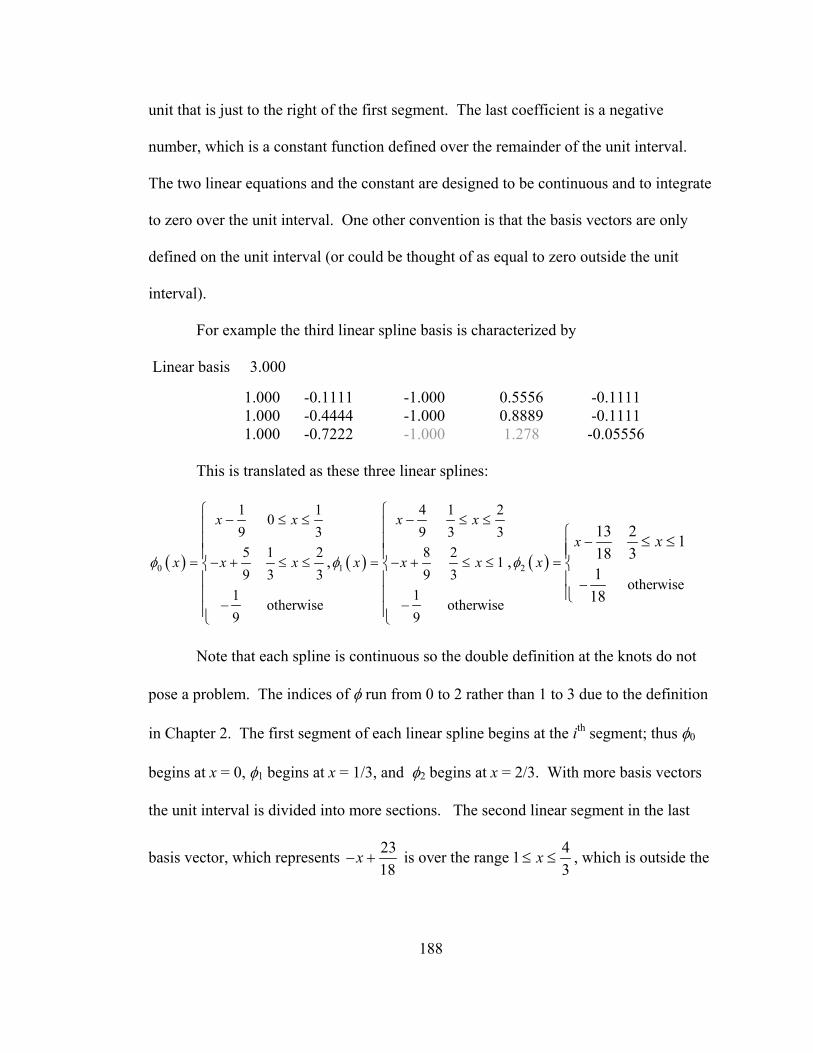
188

unit that is just to the right of the first segment. The last coefficient is a negative

number, which is a constant function defined over the remainder of the unit interval.

The two linear equations and the constant are designed to be continuous and to integrate

to zero over the unit interval. One other convention is that the basis vectors are only

defined on the unit interval (or could be thought of as equal to zero outside the unit

interval).

For example the third linear spline basis is characterized by Linear basis 3.000

1.000 -0.1111 -1.000 0.5556 -0.1111 1.000 -0.4444 -1.000 0.8889 -0.1111 1.000 -0.7222 -1.000 1.278 -0.05556

This is translated as these three linear splines:

( )0

1 10

9 35 1 29 3 3

1otherwise

9

x x

x x xφ

− ≤ ≤

= − + ≤ ≤

−

⎧⎪⎪⎪⎨⎪⎪⎪⎩

, ( )1

4 1 29 3 38 2

19 3

1otherwise

9

x x

x x xφ

− ≤ ≤

= − + ≤ ≤

−

⎧⎪⎪⎪⎨⎪⎪⎪⎩

, ( )2

otherwise

13 2 118 31

18

xx

xφ

−=

−

⎧ ≤ ≤⎪⎪⎨⎪⎪⎩

Note that each spline is continuous so the double definition at the knots do not

pose a problem. The indices of φ run from 0 to 2 rather than 1 to 3 due to the definition

in Chapter 2. The first segment of each linear spline begins at the ith segment; thus φ0

begins at x = 0, φ1 begins at x = 1/3, and φ2 begins at x = 2/3. With more basis vectors

the unit interval is divided into more sections. The second linear segment in the last

basis vector, which represents 23 4 is over the range 118 3

x x− + ≤ ≤ , which is outside the

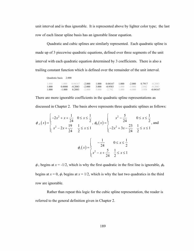
189

unit interval and is thus ignorable. It is represented above by lighter color type; the last

row of each linear spline basis has an ignorable linear equation.

Quadratic and cubic splines are similarly represented. Each quadratic spline is

made up of 3 piecewise quadratic equations, defined over three segments of the unit

interval with each quadratic equation determined by 3 coefficients. There is also a

trailing constant function which is defined over the remainder of the unit interval.

Quadratic basis 2.000 1.000 1.000 0.04167 -2.000 1.000 0.04167 1.000 -2.000 0.7917 -0.2083 1.000 0.0000 -0.2083 -2.000 3.000 -0.9583 1.000 -3.000 2.042 -0.2083 1.000 -1.000 0.2083 -2.000 5.000 -2.792 1.000 -4.000 3.958 -0.04167 There are more ignorable coefficients in the quadratic spline representations as

discussed in Chapter 2. The basis above represents three quadratic splines as follows:

( )2

12

1 12 024 2

19 12 124 2

x x xx

x x xφ−

⎧− + + ≤ ≤⎪⎪= ⎨⎪ − + ≤ ≤⎪⎩

, ( )2

02

5 1024 2

23 12 3 124 2

x xx

x x xφ

⎧ − ≤ ≤⎪⎪= ⎨⎪− + − ≤ ≤⎪⎩

, and

( )12

1 1024 2

5 1 124 2

xx

x x xφ

⎧ − ≤ ≤⎪⎪= ⎨⎪ − + ≤ ≤⎪⎩

φ-1 begins at x = -1/2, which is why the first quadratic in the first line is ignorable, φ0

begins at x = 0, φ1 begins at x = 1/2, which is why the last two quadratics in the third

row are ignorable.

Rather than repeat this logic for the cubic spline representation, the reader is

referred to the general definition given in Chapter 2.

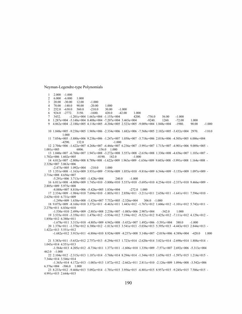
190

Neyman-Legendre-type Polynomials 1 2.000 -1.000 2 6.000 -6.000 1.000 3 20.00 -30.00 12.00 -1.000 4 70.00 -140.0 90.00 -20.00 1.000 5 252.0 -630.0 560.0 -210.0 30.00 -1.000 6 924.0 -2772. 3150. -1680. 420.0 -42.00 1.000 7 3432. -1.201e+004 1.663e+004 -1.155e+004 4200. -756.0 56.00 -1.000 8 1.287e+004 -5.148e+004 8.408e+004 -7.207e+004 3.465e+004 -9240. 1260. -72.00 1.000 9 4.862e+004 -2.188e+005 4.118e+005 -4.204e+005 2.523e+005 -9.009e+004 1.848e+004 -1980. 90.00 -1.000 10 1.848e+005 -9.238e+005 1.969e+006 -2.334e+006 1.682e+006 -7.568e+005 2.102e+005 -3.432e+004 2970. -110.0 1.000 11 7.054e+005 -3.880e+006 9.238e+006 -1.247e+007 1.050e+007 -5.718e+006 2.018e+006 -4.505e+005 6.006e+004 -4290. 132.0 -1.000 12 2.704e+006 -1.622e+007 4.268e+007 -6.466e+007 6.236e+007 -3.991e+007 1.715e+007 -4.901e+006 9.009e+005 -1.001e+005 6006. -156.0 1.000 13 1.040e+007 -6.760e+007 1.947e+008 -3.272e+008 3.557e+008 -2.619e+008 1.330e+008 -4.656e+007 1.103e+007 -1.702e+006 1.602e+005 -8190. 182.0 -1.000 14 4.012e+007 -2.808e+008 8.789e+008 -1.622e+009 1.963e+009 -1.636e+009 9.603e+008 -3.991e+008 1.164e+008 -2.328e+007 3.063e+006 -2.475e+005 1.092e+004 -210.0 1.000 15 1.551e+008 -1.163e+009 3.931e+009 -7.910e+009 1.055e+010 -9.816e+009 6.544e+009 -3.155e+009 1.097e+009 -2.716e+008 4.656e+007 -5.291e+006 3.713e+005 -1.428e+004 240.0 -1.000 16 6.011e+008 -4.809e+009 1.745e+010 -3.800e+010 5.537e+010 -5.695e+010 4.254e+010 -2.337e+010 9.466e+009 -2.805e+009 5.975e+008 -8.888e+007 8.818e+006 -5.426e+005 1.836e+004 -272.0 1.000 17 2.334e+009 -1.984e+010 7.694e+010 -1.803e+011 2.850e+011 -3.211e+011 2.658e+011 -1.641e+011 7.596e+010 -2.629e+010 6.731e+009 -1.249e+009 1.630e+008 -1.424e+007 7.752e+005 -2.326e+004 306.0 -1.000 18 9.075e+009 -8.168e+010 3.372e+011 -8.463e+011 1.443e+012 -1.767e+012 1.606e+012 -1.101e+012 5.742e+011 -2.279e+011 6.836e+010 -1.530e+010 2.499e+009 -2.883e+008 2.238e+007 -1.085e+006 2.907e+004 -342.0 1.000 19 3.535e+010 -3.358e+011 1.470e+012 -3.934e+012 7.194e+012 -9.521e+012 9.425e+012 -7.111e+012 4.129e+012 -1.850e+012 6.380e+011 -1.678e+011 3.315e+010 -4.805e+009 4.942e+008 -3.432e+007 1.492e+006 -3.591e+004 380.0 -1.000 20 1.378e+011 -1.378e+012 6.380e+012 -1.813e+013 3.541e+013 -5.036e+013 5.395e+013 -4.443e+013 2.844e+013 -1.422e+013 5.551e+012 -1.682e+012 3.915e+011 -6.884e+010 8.924e+009 -8.237e+008 5.148e+007 -2.019e+006 4.389e+004 -420.0 1.000 21 5.383e+011 -5.652e+012 2.757e+013 -8.294e+013 1.723e+014 -2.620e+014 3.021e+014 -2.698e+014 1.888e+014 -1.043e+014 4.551e+013 -1.564e+013 4.205e+012 -8.734e+011 1.377e+011 -1.606e+010 1.339e+009 -7.571e+007 2.692e+006 -5.313e+004 462.0 -1.000 22 2.104e+012 -2.315e+013 1.187e+014 -3.768e+014 8.294e+014 -1.344e+015 1.659e+015 -1.597e+015 1.214e+015 -7.344e+014 3.546e+014 -1.365e+014 4.172e+013 -1.003e+013 1.872e+012 -2.662e+011 2.811e+010 -2.126e+009 1.094e+008 -3.542e+006 6.376e+004 -506.0 1.000 23 8.233e+012 -9.468e+013 5.092e+014 -1.701e+015 3.956e+015 -6.801e+015 8.957e+015 -9.245e+015 7.586e+015 -4.991e+015 2.644e+015

191

-1.128e+015 3.868e+014 -1.059e+014 2.292e+013 -3.868e+012 4.991e+011 -4.795e+010 3.307e+009 -1.554e+008 4.605e+006 -7.590e+004 552.0 -1.000 24 3.225e+013 -3.870e+014 2.178e+015 -7.638e+015 1.871e+016 -3.402e+016 4.761e+016 -5.246e+016 4.623e+016 -3.287e+016 1.896e+016 -8.892e+015 3.385e+015 -1.041e+015 2.572e+014 -5.043e+013 7.736e+012 -9.101e+011 7.992e+010 -5.048e+009 2.176e+008 -5.920e+006 8.970e+004 -600.0 1.000 Splines: Linear basis 1.000 1.000 -0.5000 -1.000 1.500 -0.5000 Linear basis 2.000 1.000 -0.2500 -1.000 0.7500 -0.2500 1.000 -0.6250 -1.000 1.375 -0.1250 Linear basis 3.000 1.000 -0.1111 -1.000 0.5556 -0.1111 1.000 -0.4444 -1.000 0.8889 -0.1111 1.000 -0.7222 -1.000 1.278 -0.05556 Linear basis 4.000 1.000 -0.06250 -1.000 0.4375 -0.06250 1.000 -0.3125 -1.000 0.6875 -0.06250 1.000 -0.5625 -1.000 0.9375 -0.06250 1.000 -0.7813 -1.000 1.219 -0.03125 Linear basis 5.000 1.000 -0.04000 -1.000 0.3600 -0.04000 1.000 -0.2400 -1.000 0.5600 -0.04000 1.000 -0.4400 -1.000 0.7600 -0.04000 1.000 -0.6400 -1.000 0.9600 -0.04000 1.000 -0.8200 -1.000 1.180 -0.02000 Linear basis 6.000 1.000 -0.02778 -1.000 0.3056 -0.02778 1.000 -0.1944 -1.000 0.4722 -0.02778 1.000 -0.3611 -1.000 0.6389 -0.02778 1.000 -0.5278 -1.000 0.8056 -0.02778 1.000 -0.6944 -1.000 0.9722 -0.02778 1.000 -0.8472 -1.000 1.153 -0.01389 Linear basis 7.000 1.000 -0.02041 -1.000 0.2653 -0.02041 1.000 -0.1633 -1.000 0.4082 -0.02041 1.000 -0.3061 -1.000 0.5510 -0.02041 1.000 -0.4490 -1.000 0.6939 -0.02041 1.000 -0.5918 -1.000 0.8367 -0.02041 1.000 -0.7347 -1.000 0.9796 -0.02041 1.000 -0.8673 -1.000 1.133 -0.01020 Linear basis 8.000 1.000 -0.01563 -1.000 0.2344 -0.01563 1.000 -0.1406 -1.000 0.3594 -0.01563 1.000 -0.2656 -1.000 0.4844 -0.01563 1.000 -0.3906 -1.000 0.6094 -0.01563 1.000 -0.5156 -1.000 0.7344 -0.01563 1.000 -0.6406 -1.000 0.8594 -0.01563

192

1.000 -0.7656 -1.000 0.9844 -0.01563 1.000 -0.8828 -1.000 1.117 -0.007813 Linear basis 9.000 1.000 -0.01235 -1.000 0.2099 -0.01235 1.000 -0.1235 -1.000 0.3210 -0.01235 1.000 -0.2346 -1.000 0.4321 -0.01235 1.000 -0.3457 -1.000 0.5432 -0.01235 1.000 -0.4568 -1.000 0.6543 -0.01235 1.000 -0.5679 -1.000 0.7654 -0.01235 1.000 -0.6790 -1.000 0.8765 -0.01235 1.000 -0.7901 -1.000 0.9877 -0.01235 1.000 -0.8951 -1.000 1.105 -0.006173 Linear basis 10.00 1.000 -0.01000 -1.000 0.1900 -0.01000 1.000 -0.1100 -1.000 0.2900 -0.01000 1.000 -0.2100 -1.000 0.3900 -0.01000 1.000 -0.3100 -1.000 0.4900 -0.01000 1.000 -0.4100 -1.000 0.5900 -0.01000 1.000 -0.5100 -1.000 0.6900 -0.01000 1.000 -0.6100 -1.000 0.7900 -0.01000 1.000 -0.7100 -1.000 0.8900 -0.01000 1.000 -0.8100 -1.000 0.9900 -0.01000 1.000 -0.9050 -1.000 1.095 -0.005000 Linear basis 11.00 1.000 -0.008264 -1.000 0.1736 -0.008264 1.000 -0.09917 -1.000 0.2645 -0.008264 1.000 -0.1901 -1.000 0.3554 -0.008264 1.000 -0.2810 -1.000 0.4463 -0.008264 1.000 -0.3719 -1.000 0.5372 -0.008264 1.000 -0.4628 -1.000 0.6281 -0.008264 1.000 -0.5537 -1.000 0.7190 -0.008264 1.000 -0.6446 -1.000 0.8099 -0.008264 1.000 -0.7355 -1.000 0.9008 -0.008264 1.000 -0.8264 -1.000 0.9917 -0.008264 1.000 -0.9132 -1.000 1.087 -0.004132 Linear basis 12.00 1.000 -0.006944 -1.000 0.1597 -0.006944 1.000 -0.09028 -1.000 0.2431 -0.006944 1.000 -0.1736 -1.000 0.3264 -0.006944 1.000 -0.2569 -1.000 0.4097 -0.006944 1.000 -0.3403 -1.000 0.4931 -0.006944 1.000 -0.4236 -1.000 0.5764 -0.006944 1.000 -0.5069 -1.000 0.6597 -0.006944 1.000 -0.5903 -1.000 0.7431 -0.006944 1.000 -0.6736 -1.000 0.8264 -0.006944 1.000 -0.7569 -1.000 0.9097 -0.006944 1.000 -0.8403 -1.000 0.9931 -0.006944 1.000 -0.9201 -1.000 1.080 -0.003472 Linear basis 13.00 1.000 -0.005917 -1.000 0.1479 -0.005917 1.000 -0.08284 -1.000 0.2249 -0.005917 1.000 -0.1598 -1.000 0.3018 -0.005917 1.000 -0.2367 -1.000 0.3787 -0.005917 1.000 -0.3136 -1.000 0.4556 -0.005917 1.000 -0.3905 -1.000 0.5325 -0.005917 1.000 -0.4675 -1.000 0.6095 -0.005917 1.000 -0.5444 -1.000 0.6864 -0.005917 1.000 -0.6213 -1.000 0.7633 -0.005917

193

1.000 -0.6982 -1.000 0.8402 -0.005917 1.000 -0.7751 -1.000 0.9172 -0.005917 1.000 -0.8521 -1.000 0.9941 -0.005917 1.000 -0.9260 -1.000 1.074 -0.002959 Linear basis 14.00 1.000 -0.005102 -1.000 0.1378 -0.005102 1.000 -0.07653 -1.000 0.2092 -0.005102 1.000 -0.1480 -1.000 0.2806 -0.005102 1.000 -0.2194 -1.000 0.3520 -0.005102 1.000 -0.2908 -1.000 0.4235 -0.005102 1.000 -0.3622 -1.000 0.4949 -0.005102 1.000 -0.4337 -1.000 0.5663 -0.005102 1.000 -0.5051 -1.000 0.6378 -0.005102 1.000 -0.5765 -1.000 0.7092 -0.005102 1.000 -0.6480 -1.000 0.7806 -0.005102 1.000 -0.7194 -1.000 0.8520 -0.005102 1.000 -0.7908 -1.000 0.9235 -0.005102 1.000 -0.8622 -1.000 0.9949 -0.005102 1.000 -0.9311 -1.000 1.069 -0.002551 Linear basis 15.00 1.000 -0.004444 -1.000 0.1289 -0.004444 1.000 -0.07111 -1.000 0.1956 -0.004444 1.000 -0.1378 -1.000 0.2622 -0.004444 1.000 -0.2044 -1.000 0.3289 -0.004444 1.000 -0.2711 -1.000 0.3956 -0.004444 1.000 -0.3378 -1.000 0.4622 -0.004444 1.000 -0.4044 -1.000 0.5289 -0.004444 1.000 -0.4711 -1.000 0.5956 -0.004444 1.000 -0.5378 -1.000 0.6622 -0.004444 1.000 -0.6044 -1.000 0.7289 -0.004444 1.000 -0.6711 -1.000 0.7956 -0.004444 1.000 -0.7378 -1.000 0.8622 -0.004444 1.000 -0.8044 -1.000 0.9289 -0.004444 1.000 -0.8711 -1.000 0.9956 -0.004444 1.000 -0.9356 -1.000 1.064 -0.002222 Linear basis 16.00 1.000 -0.003906 -1.000 0.1211 -0.003906 1.000 -0.06641 -1.000 0.1836 -0.003906 1.000 -0.1289 -1.000 0.2461 -0.003906 1.000 -0.1914 -1.000 0.3086 -0.003906 1.000 -0.2539 -1.000 0.3711 -0.003906 1.000 -0.3164 -1.000 0.4336 -0.003906 1.000 -0.3789 -1.000 0.4961 -0.003906 1.000 -0.4414 -1.000 0.5586 -0.003906 1.000 -0.5039 -1.000 0.6211 -0.003906 1.000 -0.5664 -1.000 0.6836 -0.003906 1.000 -0.6289 -1.000 0.7461 -0.003906 1.000 -0.6914 -1.000 0.8086 -0.003906 1.000 -0.7539 -1.000 0.8711 -0.003906 1.000 -0.8164 -1.000 0.9336 -0.003906 1.000 -0.8789 -1.000 0.9961 -0.003906 1.000 -0.9395 -1.000 1.061 -0.001953 Linear basis 17.00 1.000 -0.003460 -1.000 0.1142 -0.003460 1.000 -0.06228 -1.000 0.1730 -0.003460 1.000 -0.1211 -1.000 0.2318 -0.003460 1.000 -0.1799 -1.000 0.2907 -0.003460 1.000 -0.2388 -1.000 0.3495 -0.003460 1.000 -0.2976 -1.000 0.4083 -0.003460 1.000 -0.3564 -1.000 0.4671 -0.003460

194

1.000 -0.4152 -1.000 0.5260 -0.003460 1.000 -0.4740 -1.000 0.5848 -0.003460 1.000 -0.5329 -1.000 0.6436 -0.003460 1.000 -0.5917 -1.000 0.7024 -0.003460 1.000 -0.6505 -1.000 0.7612 -0.003460 1.000 -0.7093 -1.000 0.8201 -0.003460 1.000 -0.7682 -1.000 0.8789 -0.003460 1.000 -0.8270 -1.000 0.9377 -0.003460 1.000 -0.8858 -1.000 0.9965 -0.003460 1.000 -0.9429 -1.000 1.057 -0.001730 Linear basis 18.00 1.000 -0.003086 -1.000 0.1080 -0.003086 1.000 -0.05864 -1.000 0.1636 -0.003086 1.000 -0.1142 -1.000 0.2191 -0.003086 1.000 -0.1698 -1.000 0.2747 -0.003086 1.000 -0.2253 -1.000 0.3302 -0.003086 1.000 -0.2809 -1.000 0.3858 -0.003086 1.000 -0.3364 -1.000 0.4414 -0.003086 1.000 -0.3920 -1.000 0.4969 -0.003086 1.000 -0.4475 -1.000 0.5525 -0.003086 1.000 -0.5031 -1.000 0.6080 -0.003086 1.000 -0.5586 -1.000 0.6636 -0.003086 1.000 -0.6142 -1.000 0.7191 -0.003086 1.000 -0.6698 -1.000 0.7747 -0.003086 1.000 -0.7253 -1.000 0.8302 -0.003086 1.000 -0.7809 -1.000 0.8858 -0.003086 1.000 -0.8364 -1.000 0.9414 -0.003086 1.000 -0.8920 -1.000 0.9969 -0.003086 1.000 -0.9460 -1.000 1.054 -0.001543 Linear basis 19.00 1.000 -0.002770 -1.000 0.1025 -0.002770 1.000 -0.05540 -1.000 0.1551 -0.002770 1.000 -0.1080 -1.000 0.2078 -0.002770 1.000 -0.1607 -1.000 0.2604 -0.002770 1.000 -0.2133 -1.000 0.3130 -0.002770 1.000 -0.2659 -1.000 0.3657 -0.002770 1.000 -0.3186 -1.000 0.4183 -0.002770 1.000 -0.3712 -1.000 0.4709 -0.002770 1.000 -0.4238 -1.000 0.5235 -0.002770 1.000 -0.4765 -1.000 0.5762 -0.002770 1.000 -0.5291 -1.000 0.6288 -0.002770 1.000 -0.5817 -1.000 0.6814 -0.002770 1.000 -0.6343 -1.000 0.7341 -0.002770 1.000 -0.6870 -1.000 0.7867 -0.002770 1.000 -0.7396 -1.000 0.8393 -0.002770 1.000 -0.7922 -1.000 0.8920 -0.002770 1.000 -0.8449 -1.000 0.9446 -0.002770 1.000 -0.8975 -1.000 0.9972 -0.002770 1.000 -0.9488 -1.000 1.051 -0.001385 Linear basis 20.00 1.000 -0.002500 -1.000 0.09750 -0.002500 1.000 -0.05250 -1.000 0.1475 -0.002500 1.000 -0.1025 -1.000 0.1975 -0.002500 1.000 -0.1525 -1.000 0.2475 -0.002500 1.000 -0.2025 -1.000 0.2975 -0.002500 1.000 -0.2525 -1.000 0.3475 -0.002500 1.000 -0.3025 -1.000 0.3975 -0.002500 1.000 -0.3525 -1.000 0.4475 -0.002500 1.000 -0.4025 -1.000 0.4975 -0.002500 1.000 -0.4525 -1.000 0.5475 -0.002500 1.000 -0.5025 -1.000 0.5975 -0.002500 1.000 -0.5525 -1.000 0.6475 -0.002500

195

1.000 -0.6025 -1.000 0.6975 -0.002500 1.000 -0.6525 -1.000 0.7475 -0.002500 1.000 -0.7025 -1.000 0.7975 -0.002500 1.000 -0.7525 -1.000 0.8475 -0.002500 1.000 -0.8025 -1.000 0.8975 -0.002500 1.000 -0.8525 -1.000 0.9475 -0.002500 1.000 -0.9025 -1.000 0.9975 -0.002500 1.000 -0.9512 -1.000 1.049 -0.001250 Linear basis 21.00 1.000 -0.002268 -1.000 0.09297 -0.002268 1.000 -0.04989 -1.000 0.1406 -0.002268 1.000 -0.09751 -1.000 0.1882 -0.002268 1.000 -0.1451 -1.000 0.2358 -0.002268 1.000 -0.1927 -1.000 0.2834 -0.002268 1.000 -0.2404 -1.000 0.3311 -0.002268 1.000 -0.2880 -1.000 0.3787 -0.002268 1.000 -0.3356 -1.000 0.4263 -0.002268 1.000 -0.3832 -1.000 0.4739 -0.002268 1.000 -0.4308 -1.000 0.5215 -0.002268 1.000 -0.4785 -1.000 0.5692 -0.002268 1.000 -0.5261 -1.000 0.6168 -0.002268 1.000 -0.5737 -1.000 0.6644 -0.002268 1.000 -0.6213 -1.000 0.7120 -0.002268 1.000 -0.6689 -1.000 0.7596 -0.002268 1.000 -0.7166 -1.000 0.8073 -0.002268 1.000 -0.7642 -1.000 0.8549 -0.002268 1.000 -0.8118 -1.000 0.9025 -0.002268 1.000 -0.8594 -1.000 0.9501 -0.002268 1.000 -0.9070 -1.000 0.9977 -0.002268 1.000 -0.9535 -1.000 1.046 -0.001134 Linear basis 22.00 1.000 -0.002066 -1.000 0.08884 -0.002066 1.000 -0.04752 -1.000 0.1343 -0.002066 1.000 -0.09298 -1.000 0.1798 -0.002066 1.000 -0.1384 -1.000 0.2252 -0.002066 1.000 -0.1839 -1.000 0.2707 -0.002066 1.000 -0.2293 -1.000 0.3161 -0.002066 1.000 -0.2748 -1.000 0.3616 -0.002066 1.000 -0.3202 -1.000 0.4070 -0.002066 1.000 -0.3657 -1.000 0.4525 -0.002066 1.000 -0.4112 -1.000 0.4979 -0.002066 1.000 -0.4566 -1.000 0.5434 -0.002066 1.000 -0.5021 -1.000 0.5888 -0.002066 1.000 -0.5475 -1.000 0.6343 -0.002066 1.000 -0.5930 -1.000 0.6798 -0.002066 1.000 -0.6384 -1.000 0.7252 -0.002066 1.000 -0.6839 -1.000 0.7707 -0.002066 1.000 -0.7293 -1.000 0.8161 -0.002066 1.000 -0.7748 -1.000 0.8616 -0.002066 1.000 -0.8202 -1.000 0.9070 -0.002066 1.000 -0.8657 -1.000 0.9525 -0.002066 1.000 -0.9112 -1.000 0.9979 -0.002066 1.000 -0.9556 -1.000 1.044 -0.001033 Linear basis 23.00 1.000 -0.001890 -1.000 0.08507 -0.001890 1.000 -0.04537 -1.000 0.1285 -0.001890 1.000 -0.08885 -1.000 0.1720 -0.001890 1.000 -0.1323 -1.000 0.2155 -0.001890 1.000 -0.1758 -1.000 0.2590 -0.001890 1.000 -0.2193 -1.000 0.3025 -0.001890 1.000 -0.2628 -1.000 0.3459 -0.001890 1.000 -0.3062 -1.000 0.3894 -0.001890

196

1.000 -0.3497 -1.000 0.4329 -0.001890 1.000 -0.3932 -1.000 0.4764 -0.001890 1.000 -0.4367 -1.000 0.5198 -0.001890 1.000 -0.4802 -1.000 0.5633 -0.001890 1.000 -0.5236 -1.000 0.6068 -0.001890 1.000 -0.5671 -1.000 0.6503 -0.001890 1.000 -0.6106 -1.000 0.6938 -0.001890 1.000 -0.6541 -1.000 0.7372 -0.001890 1.000 -0.6975 -1.000 0.7807 -0.001890 1.000 -0.7410 -1.000 0.8242 -0.001890 1.000 -0.7845 -1.000 0.8677 -0.001890 1.000 -0.8280 -1.000 0.9112 -0.001890 1.000 -0.8715 -1.000 0.9546 -0.001890 1.000 -0.9149 -1.000 0.9981 -0.001890 1.000 -0.9575 -1.000 1.043 -0.0009452 Linear basis 24.00 1.000 -0.001736 -1.000 0.08160 -0.001736 1.000 -0.04340 -1.000 0.1233 -0.001736 1.000 -0.08507 -1.000 0.1649 -0.001736 1.000 -0.1267 -1.000 0.2066 -0.001736 1.000 -0.1684 -1.000 0.2483 -0.001736 1.000 -0.2101 -1.000 0.2899 -0.001736 1.000 -0.2517 -1.000 0.3316 -0.001736 1.000 -0.2934 -1.000 0.3733 -0.001736 1.000 -0.3351 -1.000 0.4149 -0.001736 1.000 -0.3767 -1.000 0.4566 -0.001736 1.000 -0.4184 -1.000 0.4983 -0.001736 1.000 -0.4601 -1.000 0.5399 -0.001736 1.000 -0.5017 -1.000 0.5816 -0.001736 1.000 -0.5434 -1.000 0.6233 -0.001736 1.000 -0.5851 -1.000 0.6649 -0.001736 1.000 -0.6267 -1.000 0.7066 -0.001736 1.000 -0.6684 -1.000 0.7483 -0.001736 1.000 -0.7101 -1.000 0.7899 -0.001736 1.000 -0.7517 -1.000 0.8316 -0.001736 1.000 -0.7934 -1.000 0.8733 -0.001736 1.000 -0.8351 -1.000 0.9149 -0.001736 1.000 -0.8767 -1.000 0.9566 -0.001736 1.000 -0.9184 -1.000 0.9983 -0.001736 1.000 -0.9592 -1.000 1.041 -0.0008681 Quadratic basis 1.000 1.000 2.000 -0.3333 -2.000 2.000 -0.3333 1.000 -4.000 2.667 -1.333 1.000 0.0000 -0.3333 -2.000 6.000 -3.333 1.000 -6.000 8.667 -0.3333 Quadratic basis 2.000 1.000 1.000 0.04167 -2.000 1.000 0.04167 1.000 -2.000 0.7917 -0.2083 1.000 0.0000 -0.2083 -2.000 3.000 -0.9583 1.000 -3.000 2.042 -0.2083 1.000 -1.000 0.2083 -2.000 5.000 -2.792 1.000 -4.000 3.958 -0.04167 Quadratic basis 3.000 1.000 0.6667 0.04938 -2.000 0.6667 0.04938 1.000 -1.333 0.3827 -0.06173 1.000 0.0000 -0.07407 -2.000 2.000 -0.4074 1.000 -2.000 0.9259 -0.07407 1.000 -0.6667 0.04938 -2.000 3.333 -1.284 1.000 -2.667 1.716 -0.06173 1.000 -1.333 0.4321 -2.000 4.667 -2.568 1.000 -3.333 2.765 -0.01235 Quadratic basis 4.000 1.000 0.5000 0.03646 -2.000 0.5000 0.03646 1.000 -1.000 0.2240 -0.02604 1.000 0.0000 -0.03125 -2.000 1.500 -0.2188 1.000 -1.500 0.5313 -0.03125 1.000 -0.5000 0.03125 -2.000 2.500 -0.7188 1.000 -2.000 0.9688 -0.03125 1.000 -1.000 0.2240 -2.000 3.500 -1.464 1.000 -2.500 1.536 -0.02604 1.000 -1.500 0.5573 -2.000 4.500 -2.443 1.000 -3.000 2.245 -0.005208

197

Quadratic basis 5.000 1.000 0.4000 0.02667 -2.000 0.4000 0.02667 1.000 -0.8000 0.1467 -0.01333 1.000 0.0000 -0.01600 -2.000 1.200 -0.1360 1.000 -1.200 0.3440 -0.01600 1.000 -0.4000 0.02400 -2.000 2.000 -0.4560 1.000 -1.600 0.6240 -0.01600 1.000 -0.8000 0.1440 -2.000 2.800 -0.9360 1.000 -2.000 0.9840 -0.01600 1.000 -1.200 0.3467 -2.000 3.600 -1.573 1.000 -2.400 1.427 -0.01333 1.000 -1.600 0.6373 -2.000 4.400 -2.363 1.000 -2.800 1.957 -0.002667 Quadratic basis 6.000 1.000 0.3333 0.02006 -2.000 0.3333 0.02006 1.000 -0.6667 0.1034 -0.007716 1.000 0.0000 -0.009259 -2.000 1.000 -0.09259 1.000 -1.000 0.2407 -0.009259 1.000 -0.3333 0.01852 -2.000 1.667 -0.3148 1.000 -1.333 0.4352 -0.009259 1.000 -0.6667 0.1019 -2.000 2.333 -0.6481 1.000 -1.667 0.6852 -0.009259 1.000 -1.000 0.2407 -2.000 3.000 -1.093 1.000 -2.000 0.9907 -0.009259 1.000 -1.333 0.4367 -2.000 3.667 -1.647 1.000 -2.333 1.353 -0.007716 1.000 -1.667 0.6929 -2.000 4.333 -2.307 1.000 -2.667 1.776 -0.001543 Quadratic basis 7.000 1.000 0.2857 0.01555 -2.000 0.2857 0.01555 1.000 -0.5714 0.07677 -0.004859 1.000 0.0000 -0.005831 -2.000 0.8571 -0.06706 1.000 -0.8571 0.1778 -0.005831 1.000 -0.2857 0.01458 -2.000 1.429 -0.2303 1.000 -1.143 0.3207 -0.005831 1.000 -0.5714 0.07580 -2.000 2.000 -0.4752 1.000 -1.429 0.5044 -0.005831 1.000 -0.8571 0.1778 -2.000 2.571 -0.8017 1.000 -1.714 0.7289 -0.005831 1.000 -1.143 0.3207 -2.000 3.143 -1.210 1.000 -2.000 0.9942 -0.005831 1.000 -1.429 0.5053 -2.000 3.714 -1.699 1.000 -2.286 1.301 -0.004859 1.000 -1.714 0.7337 -2.000 4.286 -2.266 1.000 -2.571 1.652 -0.0009718 Quadratic basis 8.000 1.000 0.2500 0.01237 -2.000 0.2500 0.01237 1.000 -0.5000 0.05924 -0.003255 1.000 0.0000 -0.003906 -2.000 0.7500 -0.05078 1.000 -0.7500 0.1367 -0.003906 1.000 -0.2500 0.01172 -2.000 1.250 -0.1758 1.000 -1.000 0.2461 -0.003906 1.000 -0.5000 0.05859 -2.000 1.750 -0.3633 1.000 -1.250 0.3867 -0.003906 1.000 -0.7500 0.1367 -2.000 2.250 -0.6133 1.000 -1.500 0.5586 -0.003906 1.000 -1.000 0.2461 -2.000 2.750 -0.9258 1.000 -1.750 0.7617 -0.003906 1.000 -1.250 0.3867 -2.000 3.250 -1.301 1.000 -2.000 0.9961 -0.003906 1.000 -1.500 0.5592 -2.000 3.750 -1.738 1.000 -2.250 1.262 -0.003255 1.000 -1.750 0.7650 -2.000 4.250 -2.235 1.000 -2.500 1.562 -0.0006510 Quadratic basis 9.000 1.000 0.2222 0.01006 -2.000 0.2222 0.01006 1.000 -0.4444 0.04710 -0.002286 1.000 0.0000 -0.002743 -2.000 0.6667 -0.03978 1.000 -0.6667 0.1084 -0.002743 1.000 -0.2222 0.009602 -2.000 1.111 -0.1385 1.000 -0.8889 0.1948 -0.002743 1.000 -0.4444 0.04664 -2.000 1.556 -0.2867 1.000 -1.111 0.3059 -0.002743 1.000 -0.6667 0.1084 -2.000 2.000 -0.4842 1.000 -1.333 0.4417 -0.002743 1.000 -0.8889 0.1948 -2.000 2.444 -0.7311 1.000 -1.556 0.6022 -0.002743 1.000 -1.111 0.3059 -2.000 2.889 -1.027 1.000 -1.778 0.7874 -0.002743 1.000 -1.333 0.4417 -2.000 3.333 -1.373 1.000 -2.000 0.9973 -0.002743 1.000 -1.556 0.6027 -2.000 3.778 -1.768 1.000 -2.222 1.232 -0.002286 1.000 -1.778 0.7897 -2.000 4.222 -2.210 1.000 -2.444 1.493 -0.0004572 Quadratic basis 10.00 1.000 0.2000 0.008333 -2.000 0.2000 0.008333 1.000 -0.4000 0.03833 -0.001667 1.000 0.0000 -0.002000 -2.000 0.6000 -0.03200 1.000 -0.6000 0.08800 -0.002000 1.000 -0.2000 0.008000 -2.000 1.000 -0.1120 1.000 -0.8000 0.1580 -0.002000 1.000 -0.4000 0.03800 -2.000 1.400 -0.2320 1.000 -1.000 0.2480 -0.002000 1.000 -0.6000 0.08800 -2.000 1.800 -0.3920 1.000 -1.200 0.3580 -0.002000 1.000 -0.8000 0.1580 -2.000 2.200 -0.5920 1.000 -1.400 0.4880 -0.002000 1.000 -1.000 0.2480 -2.000 2.600 -0.8320 1.000 -1.600 0.6380 -0.002000 1.000 -1.200 0.3580 -2.000 3.000 -1.112 1.000 -1.800 0.8080 -0.002000 1.000 -1.400 0.4880 -2.000 3.400 -1.432 1.000 -2.000 0.9980 -0.002000 1.000 -1.600 0.6383 -2.000 3.800 -1.792 1.000 -2.200 1.208 -0.001667

198

1.000 -1.800 0.8097 -2.000 4.200 -2.190 1.000 -2.400 1.440 -0.0003333 Quadratic basis 11.00 1.000 0.1818 0.007012 -2.000 0.1818 0.007012 1.000 -0.3636 0.03181 -0.001252 1.000 0.0000 -0.001503 -2.000 0.5455 -0.02630 1.000 -0.5455 0.07288 -0.001503 1.000 -0.1818 0.006762 -2.000 0.9091 -0.09241 1.000 -0.7273 0.1307 -0.001503 1.000 -0.3636 0.03156 -2.000 1.273 -0.1916 1.000 -0.9091 0.2051 -0.001503 1.000 -0.5455 0.07288 -2.000 1.636 -0.3238 1.000 -1.091 0.2960 -0.001503 1.000 -0.7273 0.1307 -2.000 2.000 -0.4891 1.000 -1.273 0.4035 -0.001503 1.000 -0.9091 0.2051 -2.000 2.364 -0.6875 1.000 -1.455 0.5274 -0.001503 1.000 -1.091 0.2960 -2.000 2.727 -0.9189 1.000 -1.636 0.6679 -0.001503 1.000 -1.273 0.4035 -2.000 3.091 -1.183 1.000 -1.818 0.8249 -0.001503 1.000 -1.455 0.5274 -2.000 3.455 -1.481 1.000 -2.000 0.9985 -0.001503 1.000 -1.636 0.6682 -2.000 3.818 -1.811 1.000 -2.182 1.189 -0.001252 1.000 -1.818 0.8262 -2.000 4.182 -2.174 1.000 -2.364 1.396 -0.0002504 Quadratic basis 12.00 1.000 0.1667 0.005980 -2.000 0.1667 0.005980 1.000 -0.3333 0.02681 -0.0009645 1.000 0.0000 -0.001157 -2.000 0.5000 -0.02199 1.000 -0.5000 0.06134 -0.001157 1.000 -0.1667 0.005787 -2.000 0.8333 -0.07755 1.000 -0.6667 0.1100 -0.001157 1.000 -0.3333 0.02662 -2.000 1.167 -0.1609 1.000 -0.8333 0.1725 -0.001157 1.000 -0.5000 0.06134 -2.000 1.500 -0.2720 1.000 -1.000 0.2488 -0.001157 1.000 -0.6667 0.1100 -2.000 1.833 -0.4109 1.000 -1.167 0.3391 -0.001157 1.000 -0.8333 0.1725 -2.000 2.167 -0.5775 1.000 -1.333 0.4433 -0.001157 1.000 -1.000 0.2488 -2.000 2.500 -0.7720 1.000 -1.500 0.5613 -0.001157 1.000 -1.167 0.3391 -2.000 2.833 -0.9942 1.000 -1.667 0.6933 -0.001157 1.000 -1.333 0.4433 -2.000 3.167 -1.244 1.000 -1.833 0.8391 -0.001157 1.000 -1.500 0.5613 -2.000 3.500 -1.522 1.000 -2.000 0.9988 -0.001157 1.000 -1.667 0.6935 -2.000 3.833 -1.827 1.000 -2.167 1.173 -0.0009645 1.000 -1.833 0.8401 -2.000 4.167 -2.160 1.000 -2.333 1.361 -0.0001929 Quadratic basis 13.00 1.000 0.1538 0.005159 -2.000 0.1538 0.005159 1.000 -0.3077 0.02291 -0.0007586 1.000 0.0000 -0.0009103 -2.000 0.4615 -0.01866 1.000 -0.4615 0.05234 -0.0009103 1.000 -0.1538 0.005007 -2.000 0.7692 -0.06600 1.000 -0.6154 0.09376 -0.0009103 1.000 -0.3077 0.02276 -2.000 1.077 -0.1370 1.000 -0.7692 0.1470 -0.0009103 1.000 -0.4615 0.05234 -2.000 1.385 -0.2317 1.000 -0.9231 0.2121 -0.0009103 1.000 -0.6154 0.09376 -2.000 1.692 -0.3500 1.000 -1.077 0.2890 -0.0009103 1.000 -0.7692 0.1470 -2.000 2.000 -0.4920 1.000 -1.231 0.3778 -0.0009103 1.000 -0.9231 0.2121 -2.000 2.308 -0.6577 1.000 -1.385 0.4784 -0.0009103 1.000 -1.077 0.2890 -2.000 2.615 -0.8471 1.000 -1.538 0.5908 -0.0009103 1.000 -1.231 0.3778 -2.000 2.923 -1.060 1.000 -1.692 0.7151 -0.0009103 1.000 -1.385 0.4784 -2.000 3.231 -1.297 1.000 -1.846 0.8512 -0.0009103 1.000 -1.538 0.5908 -2.000 3.538 -1.557 1.000 -2.000 0.9991 -0.0009103 1.000 -1.692 0.7152 -2.000 3.846 -1.841 1.000 -2.154 1.159 -0.0007586 1.000 -1.846 0.8519 -2.000 4.154 -2.148 1.000 -2.308 1.331 -0.0001517 Quadratic basis 14.00 1.000 0.1429 0.004495 -2.000 0.1429 0.004495 1.000 -0.2857 0.01980 -0.0006074 1.000 0.0000 -0.0007289 -2.000 0.4286 -0.01603 1.000 -0.4286 0.04519 -0.0007289 1.000 -0.1429 0.004373 -2.000 0.7143 -0.05685 1.000 -0.5714 0.08090 -0.0007289 1.000 -0.2857 0.01968 -2.000 1.000 -0.1181 1.000 -0.7143 0.1268 -0.0007289 1.000 -0.4286 0.04519 -2.000 1.286 -0.1997 1.000 -0.8571 0.1829 -0.0007289 1.000 -0.5714 0.08090 -2.000 1.571 -0.3017 1.000 -1.000 0.2493 -0.0007289 1.000 -0.7143 0.1268 -2.000 1.857 -0.4242 1.000 -1.143 0.3258 -0.0007289 1.000 -0.8571 0.1829 -2.000 2.143 -0.5671 1.000 -1.286 0.4125 -0.0007289 1.000 -1.000 0.2493 -2.000 2.429 -0.7303 1.000 -1.429 0.5095 -0.0007289 1.000 -1.143 0.3258 -2.000 2.714 -0.9140 1.000 -1.571 0.6166 -0.0007289 1.000 -1.286 0.4125 -2.000 3.000 -1.118 1.000 -1.714 0.7340 -0.0007289 1.000 -1.429 0.5095 -2.000 3.286 -1.343 1.000 -1.857 0.8615 -0.0007289 1.000 -1.571 0.6166 -2.000 3.571 -1.587 1.000 -2.000 0.9993 -0.0007289 1.000 -1.714 0.7341 -2.000 3.857 -1.853 1.000 -2.143 1.147 -0.0006074 1.000 -1.857 0.8621 -2.000 4.143 -2.138 1.000 -2.286 1.306 -0.0001215

199

Quadratic basis 15.00 1.000 0.1333 0.003951 -2.000 0.1333 0.003951 1.000 -0.2667 0.01728 -0.0004938 1.000 0.0000 -0.0005926 -2.000 0.4000 -0.01393 1.000 -0.4000 0.03941 -0.0005926 1.000 -0.1333 0.003852 -2.000 0.6667 -0.04948 1.000 -0.5333 0.07052 -0.0005926 1.000 -0.2667 0.01719 -2.000 0.9333 -0.1028 1.000 -0.6667 0.1105 -0.0005926 1.000 -0.4000 0.03941 -2.000 1.200 -0.1739 1.000 -0.8000 0.1594 -0.0005926 1.000 -0.5333 0.07052 -2.000 1.467 -0.2628 1.000 -0.9333 0.2172 -0.0005926 1.000 -0.6667 0.1105 -2.000 1.733 -0.3695 1.000 -1.067 0.2839 -0.0005926 1.000 -0.8000 0.1594 -2.000 2.000 -0.4939 1.000 -1.200 0.3594 -0.0005926 1.000 -0.9333 0.2172 -2.000 2.267 -0.6361 1.000 -1.333 0.4439 -0.0005926 1.000 -1.067 0.2839 -2.000 2.533 -0.7961 1.000 -1.467 0.5372 -0.0005926 1.000 -1.200 0.3594 -2.000 2.800 -0.9739 1.000 -1.600 0.6394 -0.0005926 1.000 -1.333 0.4439 -2.000 3.067 -1.169 1.000 -1.733 0.7505 -0.0005926 1.000 -1.467 0.5372 -2.000 3.333 -1.383 1.000 -1.867 0.8705 -0.0005926 1.000 -1.600 0.6394 -2.000 3.600 -1.614 1.000 -2.000 0.9994 -0.0005926 1.000 -1.733 0.7506 -2.000 3.867 -1.863 1.000 -2.133 1.137 -0.0004938 1.000 -1.867 0.8710 -2.000 4.133 -2.129 1.000 -2.267 1.284 -9.877e-005 Quadratic basis 16.00 1.000 0.1250 0.003499 -2.000 0.1250 0.003499 1.000 -0.2500 0.01522 -0.0004069 1.000 0.0000 -0.0004883 -2.000 0.3750 -0.01221 1.000 -0.3750 0.03467 -0.0004883 1.000 -0.1250 0.003418 -2.000 0.6250 -0.04346 1.000 -0.5000 0.06201 -0.0004883 1.000 -0.2500 0.01514 -2.000 0.8750 -0.09033 1.000 -0.6250 0.09717 -0.0004883 1.000 -0.3750 0.03467 -2.000 1.125 -0.1528 1.000 -0.7500 0.1401 -0.0004883 1.000 -0.5000 0.06201 -2.000 1.375 -0.2310 1.000 -0.8750 0.1909 -0.0004883 1.000 -0.6250 0.09717 -2.000 1.625 -0.3247 1.000 -1.000 0.2495 -0.0004883 1.000 -0.7500 0.1401 -2.000 1.875 -0.4341 1.000 -1.125 0.3159 -0.0004883 1.000 -0.8750 0.1909 -2.000 2.125 -0.5591 1.000 -1.250 0.3901 -0.0004883 1.000 -1.000 0.2495 -2.000 2.375 -0.6997 1.000 -1.375 0.4722 -0.0004883 1.000 -1.125 0.3159 -2.000 2.625 -0.8560 1.000 -1.500 0.5620 -0.0004883 1.000 -1.250 0.3901 -2.000 2.875 -1.028 1.000 -1.625 0.6597 -0.0004883 1.000 -1.375 0.4722 -2.000 3.125 -1.215 1.000 -1.750 0.7651 -0.0004883 1.000 -1.500 0.5620 -2.000 3.375 -1.418 1.000 -1.875 0.8784 -0.0004883 1.000 -1.625 0.6597 -2.000 3.625 -1.637 1.000 -2.000 0.9995 -0.0004883 1.000 -1.750 0.7652 -2.000 3.875 -1.872 1.000 -2.125 1.128 -0.0004069 1.000 -1.875 0.8788 -2.000 4.125 -2.121 1.000 -2.250 1.266 -8.138e-005 Quadratic basis 17.00 1.000 0.1176 0.003121 -2.000 0.1176 0.003121 1.000 -0.2353 0.01350 -0.0003392 1.000 0.0000 -0.0004071 -2.000 0.3529 -0.01079 1.000 -0.3529 0.03073 -0.0004071 1.000 -0.1176 0.003053 -2.000 0.5882 -0.03847 1.000 -0.4706 0.05496 -0.0004071 1.000 -0.2353 0.01343 -2.000 0.8235 -0.07999 1.000 -0.5882 0.08610 -0.0004071 1.000 -0.3529 0.03073 -2.000 1.059 -0.1354 1.000 -0.7059 0.1242 -0.0004071 1.000 -0.4706 0.05496 -2.000 1.294 -0.2046 1.000 -0.8235 0.1691 -0.0004071 1.000 -0.5882 0.08610 -2.000 1.529 -0.2876 1.000 -0.9412 0.2210 -0.0004071 1.000 -0.7059 0.1242 -2.000 1.765 -0.3845 1.000 -1.059 0.2799 -0.0004071 1.000 -0.8235 0.1691 -2.000 2.000 -0.4952 1.000 -1.176 0.3456 -0.0004071 1.000 -0.9412 0.2210 -2.000 2.235 -0.6198 1.000 -1.294 0.4183 -0.0004071 1.000 -1.059 0.2799 -2.000 2.471 -0.7582 1.000 -1.412 0.4979 -0.0004071 1.000 -1.176 0.3456 -2.000 2.706 -0.9104 1.000 -1.529 0.5844 -0.0004071 1.000 -1.294 0.4183 -2.000 2.941 -1.077 1.000 -1.647 0.6778 -0.0004071 1.000 -1.412 0.4979 -2.000 3.176 -1.256 1.000 -1.765 0.7781 -0.0004071 1.000 -1.529 0.5844 -2.000 3.412 -1.450 1.000 -1.882 0.8854 -0.0004071 1.000 -1.647 0.6778 -2.000 3.647 -1.658 1.000 -2.000 0.9996 -0.0004071 1.000 -1.765 0.7782 -2.000 3.882 -1.879 1.000 -2.118 1.121 -0.0003392 1.000 -1.882 0.8857 -2.000 4.118 -2.114 1.000 -2.235 1.249 -6.785e-005 Quadratic basis 18.00 1.000 0.1111 0.002801 -2.000 0.1111 0.002801 1.000 -0.2222 0.01206 -0.0002858 1.000 0.0000 -0.0003429 -2.000 0.3333 -0.009602 1.000 -0.3333 0.02743 -0.0003429 1.000 -0.1111 0.002743 -2.000 0.5556 -0.03429 1.000 -0.4444 0.04904 -0.0003429 1.000 -0.2222 0.01200 -2.000 0.7778 -0.07133 1.000 -0.5556 0.07682 -0.0003429 1.000 -0.3333 0.02743 -2.000 1.000 -0.1207 1.000 -0.6667 0.1108 -0.0003429 1.000 -0.4444 0.04904 -2.000 1.222 -0.1824 1.000 -0.7778 0.1509 -0.0003429

200

1.000 -0.5556 0.07682 -2.000 1.444 -0.2565 1.000 -0.8889 0.1972 -0.0003429 1.000 -0.6667 0.1108 -2.000 1.667 -0.3429 1.000 -1.000 0.2497 -0.0003429 1.000 -0.7778 0.1509 -2.000 1.889 -0.4417 1.000 -1.111 0.3083 -0.0003429 1.000 -0.8889 0.1972 -2.000 2.111 -0.5528 1.000 -1.222 0.3731 -0.0003429 1.000 -1.000 0.2497 -2.000 2.333 -0.6763 1.000 -1.333 0.4441 -0.0003429 1.000 -1.111 0.3083 -2.000 2.556 -0.8121 1.000 -1.444 0.5213 -0.0003429 1.000 -1.222 0.3731 -2.000 2.778 -0.9602 1.000 -1.556 0.6046 -0.0003429 1.000 -1.333 0.4441 -2.000 3.000 -1.121 1.000 -1.667 0.6941 -0.0003429 1.000 -1.444 0.5213 -2.000 3.222 -1.294 1.000 -1.778 0.7898 -0.0003429 1.000 -1.556 0.6046 -2.000 3.444 -1.479 1.000 -1.889 0.8916 -0.0003429 1.000 -1.667 0.6941 -2.000 3.667 -1.676 1.000 -2.000 0.9997 -0.0003429 1.000 -1.778 0.7898 -2.000 3.889 -1.886 1.000 -2.111 1.114 -0.0002858 1.000 -1.889 0.8919 -2.000 4.111 -2.108 1.000 -2.222 1.235 -5.716e-005 Quadratic basis 19.00 1.000 0.1053 0.002527 -2.000 0.1053 0.002527 1.000 -0.2105 0.01084 -0.0002430 1.000 0.0000 -0.0002916 -2.000 0.3158 -0.008602 1.000 -0.3158 0.02464 -0.0002916 1.000 -0.1053 0.002478 -2.000 0.5263 -0.03076 1.000 -0.4211 0.04403 -0.0002916 1.000 -0.2105 0.01079 -2.000 0.7368 -0.06400 1.000 -0.5263 0.06896 -0.0002916 1.000 -0.3158 0.02464 -2.000 0.9474 -0.1083 1.000 -0.6316 0.09943 -0.0002916 1.000 -0.4211 0.04403 -2.000 1.158 -0.1637 1.000 -0.7368 0.1354 -0.0002916 1.000 -0.5263 0.06896 -2.000 1.368 -0.2302 1.000 -0.8421 0.1770 -0.0002916 1.000 -0.6316 0.09943 -2.000 1.579 -0.3078 1.000 -0.9474 0.2241 -0.0002916 1.000 -0.7368 0.1354 -2.000 1.789 -0.3964 1.000 -1.053 0.2767 -0.0002916 1.000 -0.8421 0.1770 -2.000 2.000 -0.4961 1.000 -1.158 0.3349 -0.0002916 1.000 -0.9474 0.2241 -2.000 2.211 -0.6069 1.000 -1.263 0.3986 -0.0002916 1.000 -1.053 0.2767 -2.000 2.421 -0.7288 1.000 -1.368 0.4679 -0.0002916 1.000 -1.158 0.3349 -2.000 2.632 -0.8618 1.000 -1.474 0.5426 -0.0002916 1.000 -1.263 0.3986 -2.000 2.842 -1.006 1.000 -1.579 0.6230 -0.0002916 1.000 -1.368 0.4679 -2.000 3.053 -1.161 1.000 -1.684 0.7088 -0.0002916 1.000 -1.474 0.5426 -2.000 3.263 -1.327 1.000 -1.789 0.8003 -0.0002916 1.000 -1.579 0.6230 -2.000 3.474 -1.504 1.000 -1.895 0.8972 -0.0002916 1.000 -1.684 0.7088 -2.000 3.684 -1.693 1.000 -2.000 0.9997 -0.0002916 1.000 -1.789 0.8003 -2.000 3.895 -1.892 1.000 -2.105 1.108 -0.0002430 1.000 -1.895 0.8975 -2.000 4.105 -2.103 1.000 -2.211 1.222 -4.860e-005 Quadratic basis 20.00 1.000 0.1000 0.002292 -2.000 0.1000 0.002292 1.000 -0.2000 0.009792 -0.0002083 1.000 0.0000 -0.0002500 -2.000 0.3000 -0.007750 1.000 -0.3000 0.02225 -0.0002500 1.000 -0.1000 0.002250 -2.000 0.5000 -0.02775 1.000 -0.4000 0.03975 -0.0002500 1.000 -0.2000 0.009750 -2.000 0.7000 -0.05775 1.000 -0.5000 0.06225 -0.0002500 1.000 -0.3000 0.02225 -2.000 0.9000 -0.09775 1.000 -0.6000 0.08975 -0.0002500 1.000 -0.4000 0.03975 -2.000 1.100 -0.1477 1.000 -0.7000 0.1223 -0.0002500 1.000 -0.5000 0.06225 -2.000 1.300 -0.2077 1.000 -0.8000 0.1598 -0.0002500 1.000 -0.6000 0.08975 -2.000 1.500 -0.2778 1.000 -0.9000 0.2023 -0.0002500 1.000 -0.7000 0.1223 -2.000 1.700 -0.3577 1.000 -1.000 0.2498 -0.0002500 1.000 -0.8000 0.1598 -2.000 1.900 -0.4477 1.000 -1.100 0.3023 -0.0002500 1.000 -0.9000 0.2023 -2.000 2.100 -0.5477 1.000 -1.200 0.3598 -0.0002500 1.000 -1.000 0.2498 -2.000 2.300 -0.6577 1.000 -1.300 0.4223 -0.0002500 1.000 -1.100 0.3023 -2.000 2.500 -0.7777 1.000 -1.400 0.4898 -0.0002500 1.000 -1.200 0.3598 -2.000 2.700 -0.9077 1.000 -1.500 0.5623 -0.0002500 1.000 -1.300 0.4223 -2.000 2.900 -1.048 1.000 -1.600 0.6398 -0.0002500 1.000 -1.400 0.4898 -2.000 3.100 -1.198 1.000 -1.700 0.7223 -0.0002500 1.000 -1.500 0.5623 -2.000 3.300 -1.358 1.000 -1.800 0.8098 -0.0002500 1.000 -1.600 0.6398 -2.000 3.500 -1.528 1.000 -1.900 0.9023 -0.0002500 1.000 -1.700 0.7223 -2.000 3.700 -1.708 1.000 -2.000 0.9998 -0.0002500 1.000 -1.800 0.8098 -2.000 3.900 -1.898 1.000 -2.100 1.102 -0.0002083 1.000 -1.900 0.9025 -2.000 4.100 -2.098 1.000 -2.200 1.210 -4.167e-005 Quadratic basis 21.00 1.000 0.09524 0.002088 -2.000 0.09524 0.002088 1.000 -0.1905 0.008890 -0.0001800 1.000 0.0000 -0.0002160 -2.000 0.2857 -0.007019 1.000 -0.2857 0.02019 -0.0002160 1.000 -0.09524 0.002052 -2.000 0.4762 -0.02516 1.000 -0.3810 0.03607 -0.0002160 1.000 -0.1905 0.008854 -2.000 0.6667 -0.05237 1.000 -0.4762 0.05647 -0.0002160 1.000 -0.2857 0.02019 -2.000 0.8571 -0.08865 1.000 -0.5714 0.08142 -0.0002160

201

1.000 -0.3810 0.03607 -2.000 1.048 -0.1340 1.000 -0.6667 0.1109 -0.0002160 1.000 -0.4762 0.05647 -2.000 1.238 -0.1884 1.000 -0.7619 0.1449 -0.0002160 1.000 -0.5714 0.08142 -2.000 1.429 -0.2519 1.000 -0.8571 0.1835 -0.0002160 1.000 -0.6667 0.1109 -2.000 1.619 -0.3245 1.000 -0.9524 0.2265 -0.0002160 1.000 -0.7619 0.1449 -2.000 1.810 -0.4061 1.000 -1.048 0.2742 -0.0002160 1.000 -0.8571 0.1835 -2.000 2.000 -0.4968 1.000 -1.143 0.3263 -0.0002160 1.000 -0.9524 0.2265 -2.000 2.190 -0.5966 1.000 -1.238 0.3830 -0.0002160 1.000 -1.048 0.2742 -2.000 2.381 -0.7054 1.000 -1.333 0.4442 -0.0002160 1.000 -1.143 0.3263 -2.000 2.571 -0.8233 1.000 -1.429 0.5100 -0.0002160 1.000 -1.238 0.3830 -2.000 2.762 -0.9503 1.000 -1.524 0.5803 -0.0002160 1.000 -1.333 0.4442 -2.000 2.952 -1.086 1.000 -1.619 0.6551 -0.0002160 1.000 -1.429 0.5100 -2.000 3.143 -1.232 1.000 -1.714 0.7345 -0.0002160 1.000 -1.524 0.5803 -2.000 3.333 -1.386 1.000 -1.810 0.8184 -0.0002160 1.000 -1.619 0.6551 -2.000 3.524 -1.549 1.000 -1.905 0.9068 -0.0002160 1.000 -1.714 0.7345 -2.000 3.714 -1.721 1.000 -2.000 0.9998 -0.0002160 1.000 -1.810 0.8184 -2.000 3.905 -1.903 1.000 -2.095 1.097 -0.0001800 1.000 -1.905 0.9070 -2.000 4.095 -2.093 1.000 -2.190 1.200 -3.599e-005 Quadratic basis 22.00 1.000 0.09091 0.001910 -2.000 0.09091 0.001910 1.000 -0.1818 0.008108 -0.0001565 1.000 0.0000 -0.0001878 -2.000 0.2727 -0.006386 1.000 -0.2727 0.01841 -0.0001878 1.000 -0.09091 0.001878 -2.000 0.4545 -0.02292 1.000 -0.3636 0.03287 -0.0001878 1.000 -0.1818 0.008077 -2.000 0.6364 -0.04771 1.000 -0.4545 0.05147 -0.0001878 1.000 -0.2727 0.01841 -2.000 0.8182 -0.08077 1.000 -0.5455 0.07419 -0.0001878 1.000 -0.3636 0.03287 -2.000 1.000 -0.1221 1.000 -0.6364 0.1011 -0.0001878 1.000 -0.4545 0.05147 -2.000 1.182 -0.1717 1.000 -0.7273 0.1320 -0.0001878 1.000 -0.5455 0.07419 -2.000 1.364 -0.2295 1.000 -0.8182 0.1672 -0.0001878 1.000 -0.6364 0.1011 -2.000 1.545 -0.2956 1.000 -0.9091 0.2064 -0.0001878 1.000 -0.7273 0.1320 -2.000 1.727 -0.3700 1.000 -1.000 0.2498 -0.0001878 1.000 -0.8182 0.1672 -2.000 1.909 -0.4527 1.000 -1.091 0.2973 -0.0001878 1.000 -0.9091 0.2064 -2.000 2.091 -0.5436 1.000 -1.182 0.3490 -0.0001878 1.000 -1.000 0.2498 -2.000 2.273 -0.6427 1.000 -1.273 0.4048 -0.0001878 1.000 -1.091 0.2973 -2.000 2.455 -0.7502 1.000 -1.364 0.4647 -0.0001878 1.000 -1.182 0.3490 -2.000 2.636 -0.8659 1.000 -1.455 0.5287 -0.0001878 1.000 -1.273 0.4048 -2.000 2.818 -0.9899 1.000 -1.545 0.5969 -0.0001878 1.000 -1.364 0.4647 -2.000 3.000 -1.122 1.000 -1.636 0.6692 -0.0001878 1.000 -1.455 0.5287 -2.000 3.182 -1.263 1.000 -1.727 0.7457 -0.0001878 1.000 -1.545 0.5969 -2.000 3.364 -1.411 1.000 -1.818 0.8263 -0.0001878 1.000 -1.636 0.6692 -2.000 3.545 -1.568 1.000 -1.909 0.9110 -0.0001878 1.000 -1.727 0.7457 -2.000 3.727 -1.734 1.000 -2.000 0.9998 -0.0001878 1.000 -1.818 0.8263 -2.000 3.909 -1.907 1.000 -2.091 1.093 -0.0001565 1.000 -1.909 0.9111 -2.000 4.091 -2.089 1.000 -2.182 1.190 -3.130e-005 Quadratic basis 23.00 1.000 0.08696 0.001753 -2.000 0.08696 0.001753 1.000 -0.1739 0.007424 -0.0001370 1.000 0.0000 -0.0001644 -2.000 0.2609 -0.005835 1.000 -0.2609 0.01685 -0.0001644 1.000 -0.08696 0.001726 -2.000 0.4348 -0.02096 1.000 -0.3478 0.03008 -0.0001644 1.000 -0.1739 0.007397 -2.000 0.6087 -0.04364 1.000 -0.4348 0.04709 -0.0001644 1.000 -0.2609 0.01685 -2.000 0.7826 -0.07389 1.000 -0.5217 0.06789 -0.0001644 1.000 -0.3478 0.03008 -2.000 0.9565 -0.1117 1.000 -0.6087 0.09246 -0.0001644 1.000 -0.4348 0.04709 -2.000 1.130 -0.1571 1.000 -0.6957 0.1208 -0.0001644 1.000 -0.5217 0.06789 -2.000 1.304 -0.2100 1.000 -0.7826 0.1530 -0.0001644 1.000 -0.6087 0.09246 -2.000 1.478 -0.2705 1.000 -0.8696 0.1889 -0.0001644 1.000 -0.6957 0.1208 -2.000 1.652 -0.3385 1.000 -0.9565 0.2286 -0.0001644 1.000 -0.7826 0.1530 -2.000 1.826 -0.4142 1.000 -1.043 0.2720 -0.0001644 1.000 -0.8696 0.1889 -2.000 2.000 -0.4973 1.000 -1.130 0.3193 -0.0001644 1.000 -0.9565 0.2286 -2.000 2.174 -0.5881 1.000 -1.217 0.3703 -0.0001644 1.000 -1.043 0.2720 -2.000 2.348 -0.6864 1.000 -1.304 0.4252 -0.0001644 1.000 -1.130 0.3193 -2.000 2.522 -0.7922 1.000 -1.391 0.4838 -0.0001644 1.000 -1.217 0.3703 -2.000 2.696 -0.9056 1.000 -1.478 0.5461 -0.0001644 1.000 -1.304 0.4252 -2.000 2.870 -1.027 1.000 -1.565 0.6123 -0.0001644 1.000 -1.391 0.4838 -2.000 3.043 -1.155 1.000 -1.652 0.6823 -0.0001644 1.000 -1.478 0.5461 -2.000 3.217 -1.291 1.000 -1.739 0.7560 -0.0001644 1.000 -1.565 0.6123 -2.000 3.391 -1.435 1.000 -1.826 0.8335 -0.0001644 1.000 -1.652 0.6823 -2.000 3.565 -1.586 1.000 -1.913 0.9148 -0.0001644 1.000 -1.739 0.7560 -2.000 3.739 -1.745 1.000 -2.000 0.9998 -0.0001644

202

1.000 -1.826 0.8335 -2.000 3.913 -1.911 1.000 -2.087 1.089 -0.0001370 1.000 -1.913 0.9149 -2.000 4.087 -2.085 1.000 -2.174 1.181 -2.740e-005 Cubic basis 1.000 1.000 6.000 12.00 5.250 -3.000 -6.000 0.0000 1.250 3.000 -6.000 0.0000 1.250 -1.000 6.000 -12.00 5.250 -2.750 1.000 3.000 3.000 -1.750 -3.000 3.000 3.000 -1.750 3.000 -15.00 21.00 -7.750 -1.000 9.000 -27.00 24.25 -2.750 1.000 0.0000 0.0000 -0.2500 -3.000 12.00 -12.00 3.750 3.000 -24.00 60.00 -44.25 -1.000 12.00 -48.00 63.75 -0.2500 Cubic basis 2.000 1.000 3.000 3.000 0.8125 -3.000 -3.000 0.0000 0.3125 3.000 -3.000 0.0000 0.3125 -1.000 3.000 -3.000 0.8125 -0.1875 1.000 1.500 0.7500 -0.2188 -3.000 1.500 0.7500 -0.2188 3.000 -7.500 5.250 -0.9688 -1.000 4.500 -6.750 3.031 -0.3438 1.000 0.0000 0.0000 -0.1875 -3.000 6.000 -3.000 0.3125 3.000 -12.00 15.00 -5.688 -1.000 6.000 -12.00 7.813 -0.1875 1.000 -1.500 0.7500 -0.1406 -3.000 10.50 -11.25 3.859 3.000 -16.50 29.25 -16.39 -1.000 7.500 -18.75 15.61 -0.01563 Cubic basis 3.000 1.000 2.000 1.333 0.2593 -3.000 -2.000 0.0000 0.1111 3.000 -2.000 0.0000 0.1111 -1.000 2.000 -1.333 0.2593 -0.03704 1.000 1.000 0.3333 -0.03395 -3.000 1.000 0.3333 -0.03395 3.000 -5.000 2.333 -0.2562 -1.000 3.000 -3.000 0.9290 -0.07099 1.000 0.0000 0.0000 -0.07099 -3.000 4.000 -1.333 0.07716 3.000 -8.000 6.667 -1.701 -1.000 4.000 -5.333 2.299 -0.07099 1.000 -1.000 0.3333 -0.07407 -3.000 7.000 -5.000 1.111 3.000 -11.00 13.00 -4.889 -1.000 5.000 -8.333 4.593 -0.03704 1.000 -2.000 1.333 -0.2994 -3.000 10.00 -10.67 3.701 3.000 -14.00 21.33 -10.52 -1.000 6.000 -12.00 7.997 -0.003086 Cubic basis 4.000 1.000 1.500 0.7500 0.1133 -3.000 -1.500 0.0000 0.05078 3.000 -1.500 0.0000 0.05078 -1.000 1.500 -0.7500 0.1133 -0.01172 1.000 0.7500 0.1875 -0.006836 -3.000 0.7500 0.1875 -0.006836 3.000 -3.750 1.313 -0.1006 -1.000 2.250 -1.688 0.3994 -0.02246 1.000 0.0000 0.0000 -0.02344 -3.000 3.000 -0.7500 0.03906 3.000 -6.000 3.750 -0.7109 -1.000 3.000 -3.000 0.9766 -0.02344 1.000 -0.7500 0.1875 -0.03809 -3.000 5.250 -2.813 0.4619 3.000 -8.250 7.313 -2.069 -1.000 3.750 -4.688 1.931 -0.02246 1.000 -1.500 0.7500 -0.1367 -3.000 7.500 -6.000 1.551 3.000 -10.50 12.00 -4.449 -1.000 4.500 -6.750 3.363 -0.01172 1.000 -2.250 1.688 -0.4229 -3.000 9.750 -10.31 3.577 3.000 -12.75 17.81 -8.142 -1.000 5.250 -9.188 5.358 -0.0009766

203

Cubic basis 5.000 1.000 1.200 0.4800 0.05920 -3.000 -1.200 0.0000 0.02720 3.000 -1.200 0.0000 0.02720 -1.000 1.200 -0.4800 0.05920 -0.004800 1.000 0.6000 0.1200 -0.001200 -3.000 0.6000 0.1200 -0.001200 3.000 -3.000 0.8400 -0.04920 -1.000 1.800 -1.080 0.2068 -0.009200 1.000 0.0000 0.0000 -0.009600 -3.000 2.400 -0.4800 0.02240 3.000 -4.800 2.400 -0.3616 -1.000 2.400 -1.920 0.5024 -0.009600 1.000 -0.6000 0.1200 -0.01760 -3.000 4.200 -1.800 0.2384 3.000 -6.600 4.680 -1.058 -1.000 3.000 -3.000 0.9904 -0.009600 1.000 -1.200 0.4800 -0.07320 -3.000 6.000 -3.840 0.7908 3.000 -8.400 7.680 -2.281 -1.000 3.600 -4.320 1.719 -0.009200 1.000 -1.800 1.080 -0.2208 -3.000 7.800 -6.600 1.827 3.000 -10.20 11.40 -4.173 -1.000 4.200 -5.880 2.739 -0.004800 1.000 -2.400 1.920 -0.5124 -3.000 9.600 -10.08 3.488 3.000 -12.00 15.84 -6.880 -1.000 4.800 -7.680 4.096 -0.0004000 Cubic basis 6.000 1.000 1.000 0.3333 0.03472 -3.000 -1.000 0.0000 0.01620 3.000 -1.000 0.0000 0.01620 -1.000 1.000 -0.3333 0.03472 -0.002315 1.000 0.5000 0.08333 0.0001929 -3.000 0.5000 0.08333 0.0001929 3.000 -2.500 0.5833 -0.02758 -1.000 1.500 -0.7500 0.1206 -0.004437 1.000 0.0000 0.0000 -0.004630 -3.000 2.000 -0.3333 0.01389 3.000 -4.000 1.667 -0.2083 -1.000 2.000 -1.333 0.2917 -0.004630 1.000 -0.5000 0.08333 -0.009259 -3.000 3.500 -1.250 0.1389 3.000 -5.500 3.250 -0.6111 -1.000 2.500 -2.083 0.5741 -0.004630 1.000 -1.000 0.3333 -0.04167 -3.000 5.000 -2.667 0.4583 3.000 -7.000 5.333 -1.319 -1.000 3.000 -3.000 0.9954 -0.004630 1.000 -1.500 0.7500 -0.1294 -3.000 6.500 -4.583 1.056 3.000 -8.500 7.917 -2.416 -1.000 3.500 -4.083 1.584 -0.004437 1.000 -2.000 1.333 -0.2986 -3.000 8.000 -7.000 2.016 3.000 -10.00 11.00 -3.984 -1.000 4.000 -5.333 2.368 -0.002315 1.000 -2.500 2.083 -0.5789 -3.000 9.500 -9.917 3.421 3.000 -11.50 14.58 -6.107 -1.000 4.500 -6.750 3.375 -0.0001929 Cubic basis 7.000 1.000 0.8571 0.2449 0.02207 -3.000 -0.8571 0.0000 0.01041 3.000 -0.8571 0.0000 0.01041 -1.000 0.8571 -0.2449 0.02207 -0.001249 1.000 0.4286 0.06122 0.0005206 -3.000 0.4286 0.06122 0.0005206 3.000 -2.143 0.4286 -0.01697 -1.000 1.286 -0.5510 0.07632 -0.002395 1.000 0.0000 0.0000 -0.002499 -3.000 1.714 -0.2449 0.009163 3.000 -3.429 1.224 -0.1308 -1.000 1.714 -0.9796 0.1841 -0.002499 1.000 -0.4286 0.06122 -0.005414 -3.000 3.000 -0.9184 0.08788 3.000 -4.714 2.388 -0.3844 -1.000 2.143 -1.531 0.3619 -0.002499 1.000 -0.8571 0.2449 -0.02582 -3.000 4.286 -1.959 0.2890 3.000 -6.000 3.918 -0.8305 -1.000 2.571

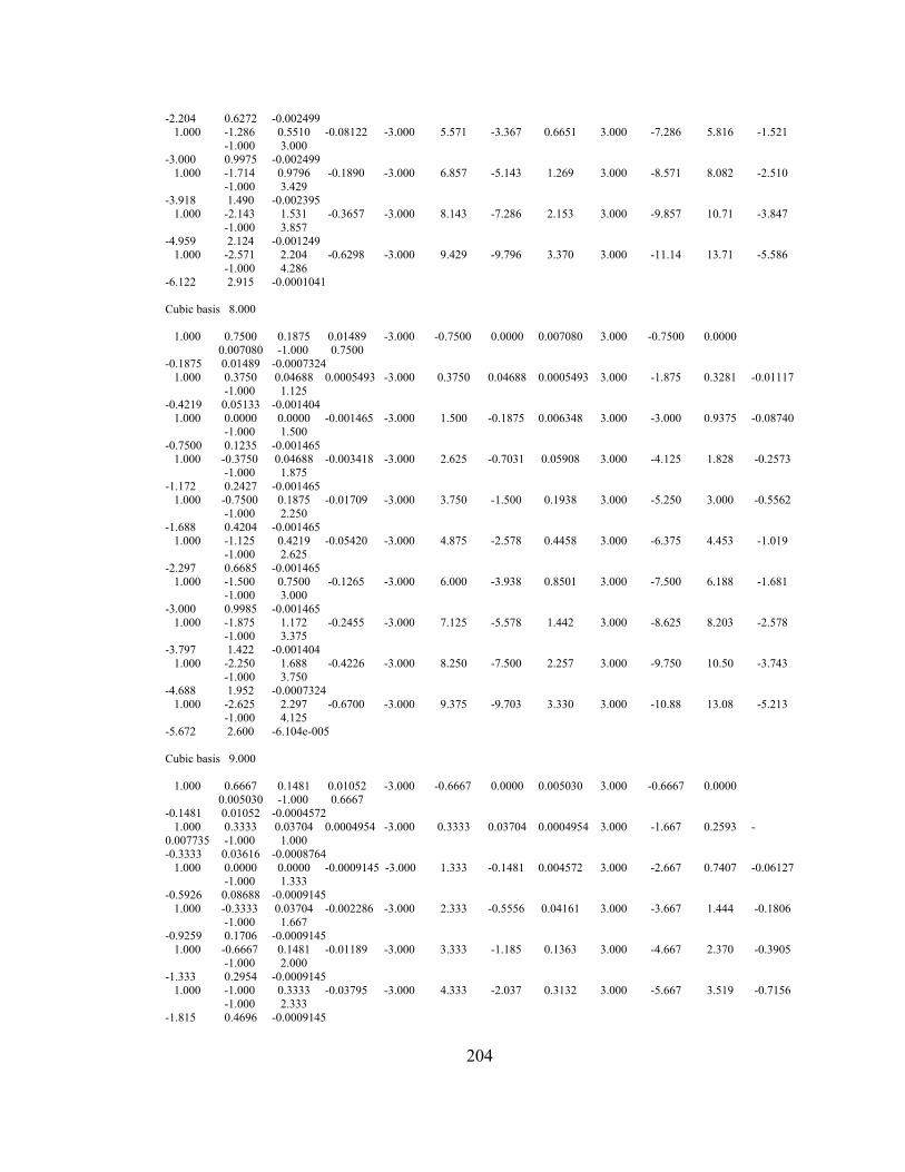
204

-2.204 0.6272 -0.002499 1.000 -1.286 0.5510 -0.08122 -3.000 5.571 -3.367 0.6651 3.000 -7.286 5.816 -1.521 -1.000 3.000 -3.000 0.9975 -0.002499 1.000 -1.714 0.9796 -0.1890 -3.000 6.857 -5.143 1.269 3.000 -8.571 8.082 -2.510 -1.000 3.429 -3.918 1.490 -0.002395 1.000 -2.143 1.531 -0.3657 -3.000 8.143 -7.286 2.153 3.000 -9.857 10.71 -3.847 -1.000 3.857 -4.959 2.124 -0.001249 1.000 -2.571 2.204 -0.6298 -3.000 9.429 -9.796 3.370 3.000 -11.14 13.71 -5.586 -1.000 4.286 -6.122 2.915 -0.0001041 Cubic basis 8.000 1.000 0.7500 0.1875 0.01489 -3.000 -0.7500 0.0000 0.007080 3.000 -0.7500 0.0000 0.007080 -1.000 0.7500 -0.1875 0.01489 -0.0007324 1.000 0.3750 0.04688 0.0005493 -3.000 0.3750 0.04688 0.0005493 3.000 -1.875 0.3281 -0.01117 -1.000 1.125 -0.4219 0.05133 -0.001404 1.000 0.0000 0.0000 -0.001465 -3.000 1.500 -0.1875 0.006348 3.000 -3.000 0.9375 -0.08740 -1.000 1.500 -0.7500 0.1235 -0.001465 1.000 -0.3750 0.04688 -0.003418 -3.000 2.625 -0.7031 0.05908 3.000 -4.125 1.828 -0.2573 -1.000 1.875 -1.172 0.2427 -0.001465 1.000 -0.7500 0.1875 -0.01709 -3.000 3.750 -1.500 0.1938 3.000 -5.250 3.000 -0.5562 -1.000 2.250 -1.688 0.4204 -0.001465 1.000 -1.125 0.4219 -0.05420 -3.000 4.875 -2.578 0.4458 3.000 -6.375 4.453 -1.019 -1.000 2.625 -2.297 0.6685 -0.001465 1.000 -1.500 0.7500 -0.1265 -3.000 6.000 -3.938 0.8501 3.000 -7.500 6.188 -1.681 -1.000 3.000 -3.000 0.9985 -0.001465 1.000 -1.875 1.172 -0.2455 -3.000 7.125 -5.578 1.442 3.000 -8.625 8.203 -2.578 -1.000 3.375 -3.797 1.422 -0.001404 1.000 -2.250 1.688 -0.4226 -3.000 8.250 -7.500 2.257 3.000 -9.750 10.50 -3.743 -1.000 3.750 -4.688 1.952 -0.0007324 1.000 -2.625 2.297 -0.6700 -3.000 9.375 -9.703 3.330 3.000 -10.88 13.08 -5.213 -1.000 4.125 -5.672 2.600 -6.104e-005 Cubic basis 9.000 1.000 0.6667 0.1481 0.01052 -3.000 -0.6667 0.0000 0.005030 3.000 -0.6667 0.0000 0.005030 -1.000 0.6667 -0.1481 0.01052 -0.0004572 1.000 0.3333 0.03704 0.0004954 -3.000 0.3333 0.03704 0.0004954 3.000 -1.667 0.2593 -0.007735 -1.000 1.000 -0.3333 0.03616 -0.0008764 1.000 0.0000 0.0000 -0.0009145 -3.000 1.333 -0.1481 0.004572 3.000 -2.667 0.7407 -0.06127 -1.000 1.333 -0.5926 0.08688 -0.0009145 1.000 -0.3333 0.03704 -0.002286 -3.000 2.333 -0.5556 0.04161 3.000 -3.667 1.444 -0.1806 -1.000 1.667 -0.9259 0.1706 -0.0009145 1.000 -0.6667 0.1481 -0.01189 -3.000 3.333 -1.185 0.1363 3.000 -4.667 2.370 -0.3905 -1.000 2.000 -1.333 0.2954 -0.0009145 1.000 -1.000 0.3333 -0.03795 -3.000 4.333 -2.037 0.3132 3.000 -5.667 3.519 -0.7156 -1.000 2.333 -1.815 0.4696 -0.0009145

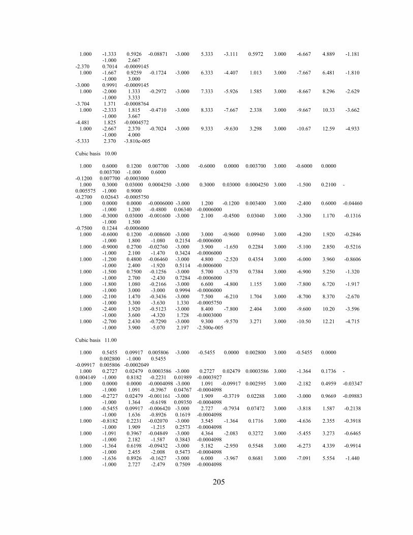
205

1.000 -1.333 0.5926 -0.08871 -3.000 5.333 -3.111 0.5972 3.000 -6.667 4.889 -1.181 -1.000 2.667 -2.370 0.7014 -0.0009145 1.000 -1.667 0.9259 -0.1724 -3.000 6.333 -4.407 1.013 3.000 -7.667 6.481 -1.810 -1.000 3.000 -3.000 0.9991 -0.0009145 1.000 -2.000 1.333 -0.2972 -3.000 7.333 -5.926 1.585 3.000 -8.667 8.296 -2.629 -1.000 3.333 -3.704 1.371 -0.0008764 1.000 -2.333 1.815 -0.4710 -3.000 8.333 -7.667 2.338 3.000 -9.667 10.33 -3.662 -1.000 3.667 -4.481 1.825 -0.0004572 1.000 -2.667 2.370 -0.7024 -3.000 9.333 -9.630 3.298 3.000 -10.67 12.59 -4.933 -1.000 4.000 -5.333 2.370 -3.810e-005 Cubic basis 10.00 1.000 0.6000 0.1200 0.007700 -3.000 -0.6000 0.0000 0.003700 3.000 -0.6000 0.0000 0.003700 -1.000 0.6000 -0.1200 0.007700 -0.0003000 1.000 0.3000 0.03000 0.0004250 -3.000 0.3000 0.03000 0.0004250 3.000 -1.500 0.2100 -0.005575 -1.000 0.9000 -0.2700 0.02643 -0.0005750 1.000 0.0000 0.0000 -0.0006000 -3.000 1.200 -0.1200 0.003400 3.000 -2.400 0.6000 -0.04460 -1.000 1.200 -0.4800 0.06340 -0.0006000 1.000 -0.3000 0.03000 -0.001600 -3.000 2.100 -0.4500 0.03040 3.000 -3.300 1.170 -0.1316 -1.000 1.500 -0.7500 0.1244 -0.0006000 1.000 -0.6000 0.1200 -0.008600 -3.000 3.000 -0.9600 0.09940 3.000 -4.200 1.920 -0.2846 -1.000 1.800 -1.080 0.2154 -0.0006000 1.000 -0.9000 0.2700 -0.02760 -3.000 3.900 -1.650 0.2284 3.000 -5.100 2.850 -0.5216 -1.000 2.100 -1.470 0.3424 -0.0006000 1.000 -1.200 0.4800 -0.06460 -3.000 4.800 -2.520 0.4354 3.000 -6.000 3.960 -0.8606 -1.000 2.400 -1.920 0.5114 -0.0006000 1.000 -1.500 0.7500 -0.1256 -3.000 5.700 -3.570 0.7384 3.000 -6.900 5.250 -1.320 -1.000 2.700 -2.430 0.7284 -0.0006000 1.000 -1.800 1.080 -0.2166 -3.000 6.600 -4.800 1.155 3.000 -7.800 6.720 -1.917 -1.000 3.000 -3.000 0.9994 -0.0006000 1.000 -2.100 1.470 -0.3436 -3.000 7.500 -6.210 1.704 3.000 -8.700 8.370 -2.670 -1.000 3.300 -3.630 1.330 -0.0005750 1.000 -2.400 1.920 -0.5123 -3.000 8.400 -7.800 2.404 3.000 -9.600 10.20 -3.596 -1.000 3.600 -4.320 1.728 -0.0003000 1.000 -2.700 2.430 -0.7290 -3.000 9.300 -9.570 3.271 3.000 -10.50 12.21 -4.715 -1.000 3.900 -5.070 2.197 -2.500e-005 Cubic basis 11.00 1.000 0.5455 0.09917 0.005806 -3.000 -0.5455 0.0000 0.002800 3.000 -0.5455 0.0000 0.002800 -1.000 0.5455 -0.09917 0.005806 -0.0002049 1.000 0.2727 0.02479 0.0003586 -3.000 0.2727 0.02479 0.0003586 3.000 -1.364 0.1736 -0.004149 -1.000 0.8182 -0.2231 0.01989 -0.0003927 1.000 0.0000 0.0000 -0.0004098 -3.000 1.091 -0.09917 0.002595 3.000 -2.182 0.4959 -0.03347 -1.000 1.091 -0.3967 0.04767 -0.0004098 1.000 -0.2727 0.02479 -0.001161 -3.000 1.909 -0.3719 0.02288 3.000 -3.000 0.9669 -0.09883 -1.000 1.364 -0.6198 0.09350 -0.0004098 1.000 -0.5455 0.09917 -0.006420 -3.000 2.727 -0.7934 0.07472 3.000 -3.818 1.587 -0.2138 -1.000 1.636 -0.8926 0.1619 -0.0004098 1.000 -0.8182 0.2231 -0.02070 -3.000 3.545 -1.364 0.1716 3.000 -4.636 2.355 -0.3918 -1.000 1.909 -1.215 0.2573 -0.0004098 1.000 -1.091 0.3967 -0.04849 -3.000 4.364 -2.083 0.3272 3.000 -5.455 3.273 -0.6465 -1.000 2.182 -1.587 0.3843 -0.0004098 1.000 -1.364 0.6198 -0.09432 -3.000 5.182 -2.950 0.5548 3.000 -6.273 4.339 -0.9914 -1.000 2.455 -2.008 0.5473 -0.0004098 1.000 -1.636 0.8926 -0.1627 -3.000 6.000 -3.967 0.8681 3.000 -7.091 5.554 -1.440 -1.000 2.727 -2.479 0.7509 -0.0004098

206

1.000 -1.909 1.215 -0.2581 -3.000 6.818 -5.132 1.281 3.000 -7.909 6.917 -2.006 -1.000 3.000 -3.000 0.9996 -0.0004098 1.000 -2.182 1.587 -0.3851 -3.000 7.636 -6.446 1.806 3.000 -8.727 8.430 -2.702 -1.000 3.273 -3.570 1.298 -0.0003927 1.000 -2.455 2.008 -0.5479 -3.000 8.455 -7.909 2.457 3.000 -9.545 10.09 -3.543 -1.000 3.545 -4.190 1.650 -0.0002049 1.000 -2.727 2.479 -0.7513 -3.000 9.273 -9.521 3.249 3.000 -10.36 11.90 -4.541 -1.000 3.818 -4.860 2.062 -1.708e-005 Cubic basis 12.00 1.000 0.5000 0.08333 0.004485 -3.000 -0.5000 0.0000 0.002170 3.000 -0.5000 0.0000 0.002170 -1.000 0.5000 -0.08333 0.004485 -0.0001447 1.000 0.2500 0.02083 0.0003014 -3.000 0.2500 0.02083 0.0003014 3.000 -1.250 0.1458 -0.003171 -1.000 0.7500 -0.1875 0.01535 -0.0002773 1.000 0.0000 0.0000 -0.0002894 -3.000 1.000 -0.08333 0.002025 3.000 -2.000 0.4167 -0.02575 -1.000 1.000 -0.3333 0.03675 -0.0002894 1.000 -0.2500 0.02083 -0.0008681 -3.000 1.750 -0.3125 0.01765 3.000 -2.750 0.8125 -0.07610 -1.000 1.250 -0.5208 0.07205 -0.0002894 1.000 -0.5000 0.08333 -0.004919 -3.000 2.500 -0.6667 0.05758 3.000 -3.500 1.333 -0.1646 -1.000 1.500 -0.7500 0.1247 -0.0002894 1.000 -0.7500 0.1875 -0.01591 -3.000 3.250 -1.146 0.1322 3.000 -4.250 1.979 -0.3018 -1.000 1.750 -1.021 0.1982 -0.0002894 1.000 -1.000 0.3333 -0.03733 -3.000 4.000 -1.750 0.2520 3.000 -5.000 2.750 -0.4980 -1.000 2.000 -1.333 0.2960 -0.0002894 1.000 -1.250 0.5208 -0.07263 -3.000 4.750 -2.479 0.4274 3.000 -5.750 3.646 -0.7636 -1.000 2.250 -1.688 0.4216 -0.0002894 1.000 -1.500 0.7500 -0.1253 -3.000 5.500 -3.333 0.6687 3.000 -6.500 4.667 -1.109 -1.000 2.500 -2.083 0.5784 -0.0002894 1.000 -1.750 1.021 -0.1988 -3.000 6.250 -4.313 0.9864 3.000 -7.250 5.813 -1.545 -1.000 2.750 -2.521 0.7700 -0.0002894 1.000 -2.000 1.333 -0.2966 -3.000 7.000 -5.417 1.391 3.000 -8.000 7.083 -2.081 -1.000 3.000 -3.000 0.9997 -0.0002894 1.000 -2.250 1.688 -0.4222 -3.000 7.750 -6.646 1.893 3.000 -8.750 8.479 -2.729 -1.000 3.250 -3.521 1.271 -0.0002773 1.000 -2.500 2.083 -0.5788 -3.000 8.500 -8.000 2.502 3.000 -9.500 10.00 -3.498 -1.000 3.500 -4.083 1.588 -0.0001447 1.000 -2.750 2.521 -0.7703 -3.000 9.250 -9.479 3.230 3.000 -10.25 11.65 -4.399 -1.000 3.750 -4.688 1.953 -1.206e-005 Cubic basis 13.00 1.000 0.4615 0.07101 0.003536 -3.000 -0.4615 0.0000 0.001716 3.000 -0.4615 0.0000 0.001716 -1.000 0.4615 -0.07101 0.003536 -0.0001050 1.000 0.2308 0.01775 0.0002538 -3.000 0.2308 0.01775 0.0002538 3.000 -1.154 0.1243 -0.002477 -1.000 0.6923 -0.1598 0.01209 -0.0002013 1.000 0.0000 0.0000 -0.0002101 -3.000 0.9231 -0.07101 0.001611 3.000 -1.846 0.3550 -0.02024 -1.000 0.9231 -0.2840 0.02892 -0.0002101 1.000 -0.2308 0.01775 -0.0006652 -3.000 1.615 -0.2663 0.01390 3.000 -2.538 0.6923 -0.05984 -1.000 1.154 -0.4438 0.05669 -0.0002101 1.000 -0.4615 0.07101 -0.003851 -3.000 2.308 -0.5680 0.04531 3.000 -3.231 1.136 -0.1295 -1.000 1.385 -0.6391 0.09811 -0.0002101 1.000 -0.6923 0.1598 -0.01250 -3.000 3.000 -0.9763 0.1040 3.000 -3.923 1.686 -0.2374 -1.000 1.615 -0.8698 0.1559 -0.0002101 1.000 -0.9231 0.2840 -0.02934 -3.000 3.692 -1.491 0.1982 3.000 -4.615 2.343 -0.3917 -1.000 1.846 -1.136 0.2328 -0.0002101 1.000 -1.154 0.4438 -0.05711 -3.000 4.385 -2.112 0.3362 3.000 -5.308 3.107 -0.6006 -1.000 2.077 -1.438 0.3316 -0.0002101 1.000 -1.385 0.6391 -0.09853 -3.000 5.077 -2.840 0.5260 3.000 -6.000 3.976 -0.8723 -1.000 2.308 -1.775 0.4550 -0.0002101 1.000 -1.615 0.8698 -0.1563 -3.000 5.769 -3.675 0.7758 3.000 -6.692 4.953 -1.215 -1.000 2.538 -2.148 0.6056 -0.0002101 1.000 -1.846 1.136 -0.2333 -3.000 6.462 -4.615 1.094 3.000 -7.385 6.036 -1.637 -1.000 2.769 -2.556 0.7863 -0.0002101 1.000 -2.077 1.438 -0.3320 -3.000 7.154 -5.663 1.489 3.000 -8.077 7.225 -2.146 -1.000 3.000 -3.000 0.9998 -0.0002101

207

1.000 -2.308 1.775 -0.4554 -3.000 7.846 -6.817 1.968 3.000 -8.769 8.521 -2.751 -1.000 3.231 -3.479 1.249 -0.0002013 1.000 -2.538 2.148 -0.6059 -3.000 8.538 -8.077 2.540 3.000 -9.462 9.923 -3.460 -1.000 3.462 -3.994 1.536 -0.0001050 1.000 -2.769 2.556 -0.7865 -3.000 9.231 -9.444 3.213 3.000 -10.15 11.43 -4.280 -1.000 3.692 -4.544 1.864 -8.753e-006 Cubic basis 14.00 1.000 0.4286 0.06122 0.002837 -3.000 -0.4286 0.0000 0.001380 3.000 -0.4286 0.0000 0.001380 -1.000 0.4286 -0.06122 0.002837 -7.809e-005 1.000 0.2143 0.01531 0.0002148 -3.000 0.2143 0.01531 0.0002148 3.000 -1.071 0.1071 -0.001972 -1.000 0.6429 -0.1378 0.009690 -0.0001497 1.000 0.0000 0.0000 -0.0001562 -3.000 0.8571 -0.06122 0.001302 3.000 -1.714 0.3061 -0.01619 -1.000 0.8571 -0.2449 0.02317 -0.0001562 1.000 -0.2143 0.01531 -0.0005206 -3.000 1.500 -0.2296 0.01114 3.000 -2.357 0.5969 -0.04790 -1.000 1.071 -0.3827 0.04540 -0.0001562 1.000 -0.4286 0.06122 -0.003072 -3.000 2.143 -0.4898 0.03629 3.000 -3.000 0.9796 -0.1037 -1.000 1.286 -0.5510 0.07856 -0.0001562 1.000 -0.6429 0.1378 -0.009996 -3.000 2.786 -0.8418 0.08330 3.000 -3.643 1.454 -0.1900 -1.000 1.500 -0.7500 0.1248 -0.0001562 1.000 -0.8571 0.2449 -0.02348 -3.000 3.429 -1.286 0.1587 3.000 -4.286 2.020 -0.3136 -1.000 1.714 -0.9796 0.1864 -0.0001562 1.000 -1.071 0.3827 -0.04571 -3.000 4.071 -1.821 0.2692 3.000 -4.929 2.679 -0.4808 -1.000 1.929 -1.240 0.2655 -0.0001562 1.000 -1.286 0.5510 -0.07887 -3.000 4.714 -2.449 0.4211 3.000 -5.571 3.429 -0.6984 -1.000 2.143 -1.531 0.3643 -0.0001562 1.000 -1.500 0.7500 -0.1252 -3.000 5.357 -3.168 0.6212 3.000 -6.214 4.270 -0.9728 -1.000 2.357 -1.852 0.4849 -0.0001562 1.000 -1.714 0.9796 -0.1867 -3.000 6.000 -3.980 0.8759 3.000 -6.857 5.204 -1.311 -1.000 2.571 -2.204 0.6296 -0.0001562 1.000 -1.929 1.240 -0.2658 -3.000 6.643 -4.883 1.192 3.000 -7.500 6.230 -1.718 -1.000 2.786 -2.587 0.8005 -0.0001562 1.000 -2.143 1.531 -0.3646 -3.000 7.286 -5.878 1.576 3.000 -8.143 7.347 -2.203 -1.000 3.000 -3.000 0.9998 -0.0001562 1.000 -2.357 1.852 -0.4852 -3.000 7.929 -6.964 2.034 3.000 -8.786 8.556 -2.770 -1.000 3.214 -3.444 1.230 -0.0001497 1.000 -2.571 2.204 -0.6298 -3.000 8.571 -8.143 2.573 3.000 -9.429 9.857 -3.427 -1.000 3.429 -3.918 1.493 -7.809e-005 1.000 -2.786 2.587 -0.8007 -3.000 9.214 -9.413 3.199 3.000 -10.07 11.25 -4.180 -1.000 3.643 -4.423 1.790 -6.508e-006 Cubic basis 15.00 1.000 0.4000 0.05333 0.002311 -3.000 -0.4000 0.0000 0.001126 3.000 -0.4000 0.0000 0.001126 -1.000 0.4000 -0.05333 0.002311 -5.926e-005 1.000 0.2000 0.01333 0.0001827 -3.000 0.2000 0.01333 0.0001827 3.000 -1.000 0.09333 -0.001595 -1.000 0.6000 -0.1200 0.007886 -0.0001136 1.000 0.0000 0.0000 -0.0001185 -3.000 0.8000 -0.05333 0.001067 3.000 -1.600 0.2667 -0.01316 -1.000 0.8000 -0.2133 0.01884 -0.0001185 1.000 -0.2000 0.01333 -0.0004148 -3.000 1.400 -0.2000 0.009067 3.000 -2.200 0.5200 -0.03893 -1.000 1.000 -0.3333 0.03692 -0.0001185 1.000 -0.4000 0.05333 -0.002489 -3.000 2.000 -0.4267 0.02951 3.000 -2.800 0.8533 -0.08427 -1.000 1.200 -0.4800 0.06388 -0.0001185 1.000 -0.6000 0.1200 -0.008119 -3.000 2.600 -0.7333 0.06773 3.000 -3.400 1.267 -0.1545 -1.000 1.400 -0.6533 0.1015 -0.0001185 1.000 -0.8000 0.2133 -0.01908 -3.000 3.200 -1.120 0.1291 3.000 -4.000 1.760 -0.2549 -1.000 1.600 -0.8533 0.1516 -0.0001185 1.000 -1.000 0.3333 -0.03716 -3.000 3.800 -1.587 0.2188 3.000 -4.600 2.333 -0.3909 -1.000 1.800 -1.080 0.2159 -0.0001185 1.000 -1.200 0.4800 -0.06412 -3.000 4.400 -2.133 0.3424 3.000 -5.200 2.987 -0.5678 -1.000 2.000 -1.333 0.2962 -0.0001185 1.000 -1.400 0.6533 -0.1017 -3.000 5.000 -2.760 0.5051 3.000 -5.800 3.720 -0.7909 -1.000 2.200 -1.613 0.3943 -0.0001185 1.000 -1.600 0.8533 -0.1518 -3.000 5.600 -3.467 0.7122 3.000 -6.400 4.533 -1.066 -1.000 2.400 -1.920 0.5119 -0.0001185

208

1.000 -1.800 1.080 -0.2161 -3.000 6.200 -4.253 0.9691 3.000 -7.000 5.427 -1.397 -1.000 2.600 -2.253 0.6508 -0.0001185 1.000 -2.000 1.333 -0.2964 -3.000 6.800 -5.120 1.281 3.000 -7.600 6.400 -1.791 -1.000 2.800 -2.613 0.8129 -0.0001185 1.000 -2.200 1.613 -0.3945 -3.000 7.400 -6.067 1.654 3.000 -8.200 7.453 -2.252 -1.000 3.000 -3.000 0.9999 -0.0001185 1.000 -2.400 1.920 -0.5121 -3.000 8.000 -7.093 2.092 3.000 -8.800 8.587 -2.786 -1.000 3.200 -3.413 1.214 -0.0001136 1.000 -2.600 2.253 -0.6510 -3.000 8.600 -8.200 2.601 3.000 -9.400 9.800 -3.399 -1.000 3.400 -3.853 1.456 -5.926e-005 1.000 -2.800 2.613 -0.8130 -3.000 9.200 -9.387 3.187 3.000 -10.00 11.09 -4.095 -1.000 3.600 -4.320 1.728 -4.938e-006 Cubic basis 16.00 1.000 0.3750 0.04688 0.001907 -3.000 -0.3750 0.0000 0.0009308 3.000 -0.3750 0.0000 0.0009308 -1.000 0.3750 -0.04688 0.001907 -4.578e-005 1.000 0.1875 0.01172 0.0001564 -3.000 0.1875 0.01172 0.0001564 3.000 -0.9375 0.08203 -0.001308 -1.000 0.5625 -0.1055 0.006504 -8.774e-005 1.000 0.0000 0.0000 -9.155e-005 -3.000 0.7500 -0.04688 0.0008850 3.000 -1.500 0.2344 -0.01083 -1.000 0.7500 -0.1875 0.01553 -9.155e-005 1.000 -0.1875 0.01172 -0.0003357 -3.000 1.313 -0.1758 0.007477 3.000 -2.063 0.4570 -0.03207 -1.000 0.9375 -0.2930 0.03043 -9.155e-005 1.000 -0.3750 0.04688 -0.002045 -3.000 1.875 -0.3750 0.02432 3.000 -2.625 0.7500 -0.06943 -1.000 1.125 -0.4219 0.05264 -9.155e-005 1.000 -0.5625 0.1055 -0.006683 -3.000 2.438 -0.6445 0.05582 3.000 -3.188 1.113 -0.1273 -1.000 1.313 -0.5742 0.08365 -9.155e-005 1.000 -0.7500 0.1875 -0.01572 -3.000 3.000 -0.9844 0.1064 3.000 -3.750 1.547 -0.2101 -1.000 1.500 -0.7500 0.1249 -9.155e-005 1.000 -0.9375 0.2930 -0.03061 -3.000 3.563 -1.395 0.1803 3.000 -4.313 2.051 -0.3221 -1.000 1.688 -0.9492 0.1779 -9.155e-005 1.000 -1.125 0.4219 -0.05283 -3.000 4.125 -1.875 0.2821 3.000 -4.875 2.625 -0.4679 -1.000 1.875 -1.172 0.2440 -9.155e-005 1.000 -1.313 0.5742 -0.08383 -3.000 4.688 -2.426 0.4162 3.000 -5.438 3.270 -0.6517 -1.000 2.063 -1.418 0.3249 -9.155e-005 1.000 -1.500 0.7500 -0.1251 -3.000 5.250 -3.047 0.5868 3.000 -6.000 3.984 -0.8780 -1.000 2.250 -1.688 0.4218 -9.155e-005 1.000 -1.688 0.9492 -0.1781 -3.000 5.813 -3.738 0.7985 3.000 -6.563 4.770 -1.151 -1.000 2.438 -1.980 0.5363 -9.155e-005 1.000 -1.875 1.172 -0.2442 -3.000 6.375 -4.500 1.056 3.000 -7.125 5.625 -1.476 -1.000 2.625 -2.297 0.6698 -9.155e-005 1.000 -2.063 1.418 -0.3250 -3.000 6.938 -5.332 1.362 3.000 -7.688 6.551 -1.856 -1.000 2.813 -2.637 0.8239 -9.155e-005 1.000 -2.250 1.688 -0.4220 -3.000 7.500 -6.234 1.724 3.000 -8.250 7.547 -2.296 -1.000 3.000 -3.000 0.9999 -9.155e-005 1.000 -2.438 1.980 -0.5365 -3.000 8.063 -7.207 2.143 3.000 -8.813 8.613 -2.801 -1.000 3.188 -3.387 1.199 -8.774e-005 1.000 -2.625 2.297 -0.6700 -3.000 8.625 -8.250 2.626 3.000 -9.375 9.750 -3.374 -1.000 3.375 -3.797 1.424 -4.578e-005 1.000 -2.813 2.637 -0.8240 -3.000 9.188 -9.363 3.176 3.000 -9.938 10.96 -4.021 -1.000 3.563 -4.230 1.675 -3.815e-006 Cubic basis 17.00 1.000 0.3529 0.04152 0.001592 -3.000 -0.3529 0.0000 0.0007782 3.000 -0.3529 0.0000 0.0007782 -1.000 0.3529 -0.04152 0.001592 -3.592e-005 1.000 0.1765 0.01038 0.0001347 -3.000 0.1765 0.01038 0.0001347 3.000 -0.8824 0.07266 -0.001087 -1.000 0.5294 -0.09343 0.005427 -6.884e-005 1.000 0.0000 0.0000 -7.184e-005 -3.000 0.7059 -0.04152 0.0007423 3.000 -1.412 0.2076 -0.009028 -1.000 0.7059 -0.1661 0.01295 -7.184e-005 1.000 -0.1765 0.01038 -0.0002754 -3.000 1.235 -0.1557 0.006238 3.000 -1.941 0.4048 -0.02674 -1.000 0.8824 -0.2595 0.02537 -7.184e-005 1.000 -0.3529 0.04152 -0.001700 -3.000 1.765 -0.3322 0.02028 3.000 -2.471 0.6644 -0.05788 -1.000 1.059 -0.3737 0.04389 -7.184e-005

209

1.000 -0.5294 0.09343 -0.005567 -3.000 2.294 -0.5709 0.04654 3.000 -3.000 0.9862 -0.1061 -1.000 1.235 -0.5087 0.06974 -7.184e-005 1.000 -0.7059 0.1661 -0.01310 -3.000 2.824 -0.8720 0.08867 3.000 -3.529 1.370 -0.1751 -1.000 1.412 -0.6644 0.1041 -7.184e-005 1.000 -0.8824 0.2595 -0.02551 -3.000 3.353 -1.235 0.1503 3.000 -4.059 1.817 -0.2685 -1.000 1.588 -0.8408 0.1483 -7.184e-005 1.000 -1.059 0.3737 -0.04404 -3.000 3.882 -1.661 0.2352 3.000 -4.588 2.325 -0.3901 -1.000 1.765 -1.038 0.2035 -7.184e-005 1.000 -1.235 0.5087 -0.06989 -3.000 4.412 -2.149 0.3470 3.000 -5.118 2.896 -0.5433 -1.000 1.941 -1.256 0.2708 -7.184e-005 1.000 -1.412 0.6644 -0.1043 -3.000 4.941 -2.699 0.4892 3.000 -5.647 3.529 -0.7320 -1.000 2.118 -1.495 0.3516 -7.184e-005 1.000 -1.588 0.8408 -0.1485 -3.000 5.471 -3.311 0.6657 3.000 -6.176 4.225 -0.9598 -1.000 2.294 -1.754 0.4471 -7.184e-005 1.000 -1.765 1.038 -0.2036 -3.000 6.000 -3.986 0.8800 3.000 -6.706 4.983 -1.230 -1.000 2.471 -2.035 0.5584 -7.184e-005 1.000 -1.941 1.256 -0.2710 -3.000 6.529 -4.723 1.136 3.000 -7.235 5.803 -1.547 -1.000 2.647 -2.336 0.6869 -7.184e-005 1.000 -2.118 1.495 -0.3518 -3.000 7.059 -5.522 1.437 3.000 -7.765 6.685 -1.914 -1.000 2.824 -2.657 0.8336 -7.184e-005 1.000 -2.294 1.754 -0.4473 -3.000 7.588 -6.384 1.787 3.000 -8.294 7.630 -2.335 -1.000 3.000 -3.000 0.9999 -7.184e-005 1.000 -2.471 2.035 -0.5586 -3.000 8.118 -7.308 2.189 3.000 -8.824 8.637 -2.813 -1.000 3.176 -3.363 1.187 -6.884e-005 1.000 -2.647 2.336 -0.6870 -3.000 8.647 -8.294 2.648 3.000 -9.353 9.706 -3.352 -1.000 3.353 -3.747 1.396 -3.592e-005 1.000 -2.824 2.657 -0.8337 -3.000 9.176 -9.343 3.166 3.000 -9.882 10.84 -3.956 -1.000 3.529 -4.152 1.628 -2.993e-006 Cubic basis 18.00 1.000 0.3333 0.03704 0.001343 -3.000 -0.3333 0.0000 0.0006573 3.000 -0.3333 0.0000 0.0006573 -1.000 0.3333 -0.03704 0.001343 -2.858e-005 1.000 0.1667 0.009259 0.0001167 -3.000 0.1667 0.009259 0.0001167 3.000 -0.8333 0.06481 -0.0009121 -1.000 0.5000 -0.08333 0.004575 -5.477e-005 1.000 0.0000 0.0000 -5.716e-005 -3.000 0.6667 -0.03704 0.0006287 3.000 -1.333 0.1852 -0.007602 -1.000 0.6667 -0.1481 0.01092 -5.716e-005 1.000 -0.1667 0.009259 -0.0002286 -3.000 1.167 -0.1389 0.005258 3.000 -1.833 0.3611 -0.02252 -1.000 0.8333 -0.2315 0.02138 -5.716e-005 1.000 -0.3333 0.03704 -0.001429 -3.000 1.667 -0.2963 0.01709 3.000 -2.333 0.5926 -0.04875 -1.000 1.000 -0.3333 0.03698 -5.716e-005 1.000 -0.5000 0.08333 -0.004687 -3.000 2.167 -0.5093 0.03921 3.000 -2.833 0.8796 -0.08939 -1.000 1.167 -0.4537 0.05876 -5.716e-005 1.000 -0.6667 0.1481 -0.01103 -3.000 2.667 -0.7778 0.07470 3.000 -3.333 1.222 -0.1475 -1.000 1.333 -0.5926 0.08773 -5.716e-005 1.000 -0.8333 0.2315 -0.02149 -3.000 3.167 -1.102 0.1267 3.000 -3.833 1.620 -0.2262 -1.000 1.500 -0.7500 0.1249 -5.716e-005 1.000 -1.000 0.3333 -0.03709 -3.000 3.667 -1.481 0.1982 3.000 -4.333 2.074 -0.3286 -1.000 1.667 -0.9259 0.1714 -5.716e-005 1.000 -1.167 0.4537 -0.05887 -3.000 4.167 -1.917 0.2923 3.000 -4.833 2.583 -0.4577 -1.000 1.833 -1.120 0.2282 -5.716e-005 1.000 -1.333 0.5926 -0.08785 -3.000 4.667 -2.407 0.4122 3.000 -5.333 3.148 -0.6167 -1.000 2.000 -1.333 0.2962 -5.716e-005 1.000 -1.500 0.7500 -0.1251 -3.000 5.167 -2.954 0.5608 3.000 -5.833 3.769 -0.8085 -1.000 2.167 -1.565 0.3767 -5.716e-005 1.000 -1.667 0.9259 -0.1715 -3.000 5.667 -3.556 0.7414 3.000 -6.333 4.444 -1.036 -1.000 2.333 -1.815 0.4705 -5.716e-005 1.000 -1.833 1.120 -0.2283 -3.000 6.167 -4.213 0.9569 3.000 -6.833 5.176 -1.303 -1.000 2.500 -2.083 0.5786 -5.716e-005 1.000 -2.000 1.333 -0.2964 -3.000 6.667 -4.926 1.211 3.000 -7.333 5.963 -1.613 -1.000 2.667 -2.370 0.7023 -5.716e-005 1.000 -2.167 1.565 -0.3768 -3.000 7.167 -5.694 1.505 3.000 -7.833 6.806 -1.967 -1.000 2.833 -2.676 0.8424 -5.716e-005 1.000 -2.333 1.815 -0.4706 -3.000 7.667 -6.519 1.844 3.000 -8.333 7.704 -2.370 -1.000 3.000 -3.000 0.9999 -5.716e-005

210

1.000 -2.500 2.083 -0.5788 -3.000 8.167 -7.398 2.231 3.000 -8.833 8.657 -2.824 -1.000 3.167 -3.343 1.176 -5.477e-005 1.000 -2.667 2.370 -0.7024 -3.000 8.667 -8.333 2.667 3.000 -9.333 9.667 -3.333 -1.000 3.333 -3.704 1.372 -2.858e-005 1.000 -2.833 2.676 -0.8424 -3.000 9.167 -9.324 3.158 3.000 -9.833 10.73 -3.899 -1.000 3.500 -4.083 1.588 -2.381e-006 Cubic basis 19.00 1.000 0.3158 0.03324 0.001143 -3.000 -0.3158 0.0000 0.0005602 3.000 -0.3158 0.0000 0.0005602 -1.000 0.3158 -0.03324 0.001143 -2.302e-005 1.000 0.1579 0.008310 0.0001017 -3.000 0.1579 0.008310 0.0001017 3.000 -0.7895 0.05817 -0.0007731 -1.000 0.4737 -0.07479 0.003892 -4.412e-005 1.000 0.0000 0.0000 -4.604e-005 -3.000 0.6316 -0.03324 0.0005371 3.000 -1.263 0.1662 -0.006461 -1.000 0.6316 -0.1330 0.009285 -4.604e-005 1.000 -0.1579 0.008310 -0.0001918 -3.000 1.105 -0.1247 0.004474 3.000 -1.737 0.3241 -0.01915 -1.000 0.7895 -0.2078 0.01818 -4.604e-005 1.000 -0.3158 0.03324 -0.001212 -3.000 1.579 -0.2659 0.01453 3.000 -2.211 0.5319 -0.04145 -1.000 0.9474 -0.2992 0.03145 -4.604e-005 1.000 -0.4737 0.07479 -0.003982 -3.000 2.053 -0.4571 0.03334 3.000 -2.684 0.7895 -0.07600 -1.000 1.105 -0.4072 0.04996 -4.604e-005 1.000 -0.6316 0.1330 -0.009377 -3.000 2.526 -0.6981 0.06352 3.000 -3.158 1.097 -0.1254 -1.000 1.263 -0.5319 0.07460 -4.604e-005 1.000 -0.7895 0.2078 -0.01827 -3.000 3.000 -0.9889 0.1077 3.000 -3.632 1.454 -0.1923 -1.000 1.421 -0.6731 0.1062 -4.604e-005 1.000 -0.9474 0.2992 -0.03154 -3.000 3.474 -1.330 0.1685 3.000 -4.105 1.861 -0.2794 -1.000 1.579 -0.8310 0.1457 -4.604e-005 1.000 -1.105 0.4072 -0.05005 -3.000 3.947 -1.720 0.2485 3.000 -4.579 2.319 -0.3892 -1.000 1.737 -1.006 0.1940 -4.604e-005 1.000 -1.263 0.5319 -0.07469 -3.000 4.421 -2.161 0.3504 3.000 -5.053 2.825 -0.5243 -1.000 1.895 -1.197 0.2519 -4.604e-005 1.000 -1.421 0.6731 -0.1063 -3.000 4.895 -2.651 0.4768 3.000 -5.526 3.382 -0.6875 -1.000 2.053 -1.404 0.3203 -4.604e-005 1.000 -1.579 0.8310 -0.1458 -3.000 5.368 -3.191 0.6304 3.000 -6.000 3.989 -0.8812 -1.000 2.211 -1.629 0.4000 -4.604e-005 1.000 -1.737 1.006 -0.1941 -3.000 5.842 -3.781 0.8136 3.000 -6.474 4.645 -1.108 -1.000 2.368 -1.870 0.4920 -4.604e-005 1.000 -1.895 1.197 -0.2520 -3.000 6.316 -4.421 1.029 3.000 -6.947 5.352 -1.371 -1.000 2.526 -2.127 0.5971 -4.604e-005 1.000 -2.053 1.404 -0.3204 -3.000 6.789 -5.111 1.280 3.000 -7.421 6.108 -1.672 -1.000 2.684 -2.402 0.7162 -4.604e-005 1.000 -2.211 1.629 -0.4001 -3.000 7.263 -5.850 1.568 3.000 -7.895 6.914 -2.015 -1.000 2.842 -2.693 0.8502 -4.604e-005 1.000 -2.368 1.870 -0.4921 -3.000 7.737 -6.640 1.897 3.000 -8.368 7.770 -2.401 -1.000 3.000 -3.000 1.000 -4.604e-005 1.000 -2.526 2.127 -0.5972 -3.000 8.211 -7.479 2.268 3.000 -8.842 8.676 -2.834 -1.000 3.158 -3.324 1.166 -4.412e-005 1.000 -2.684 2.402 -0.7163 -3.000 8.684 -8.368 2.685 3.000 -9.316 9.632 -3.315 -1.000 3.316 -3.665 1.350 -2.302e-005 1.000 -2.842 2.693 -0.8503 -3.000 9.158 -9.307 3.150 3.000 -9.789 10.64 -3.848 -1.000 3.474 -4.022 1.552 -1.918e-006 Cubic basis 20.00 1.000 0.3000 0.03000 0.0009812 -3.000 -0.3000 0.0000 0.0004813 3.000 -0.3000 0.0000 0.0004813 -1.000 0.3000 -0.03000 0.0009812 -1.875e-005 1.000 0.1500 0.007500 8.906e-005 -3.000 0.1500 0.007500 8.906e-005 3.000 -0.7500 0.05250 -0.0006609 -1.000 0.4500 -0.06750 0.003339 -3.594e-005 1.000 0.0000 0.0000 -3.750e-005 -3.000 0.6000 -0.03000 0.0004625 3.000 -1.200 0.1500 -0.005537 -1.000 0.6000 -0.1200 0.007963 -3.750e-005 1.000 -0.1500 0.007500 -0.0001625 -3.000 1.050 -0.1125 0.003837 3.000 -1.650 0.2925 -0.01641 -1.000 0.7500 -0.1875 0.01559 -3.750e-005 1.000 -0.3000 0.03000 -0.001038 -3.000 1.500 -0.2400 0.01246 3.000 -2.100 0.4800 -0.03554 -1.000 0.9000 -0.2700 0.02696 -3.750e-005

211

1.000 -0.4500 0.06750 -0.003413 -3.000 1.950 -0.4125 0.02859 3.000 -2.550 0.7125 -0.06516 -1.000 1.050 -0.3675 0.04284 -3.750e-005 1.000 -0.6000 0.1200 -0.008037 -3.000 2.400 -0.6300 0.05446 3.000 -3.000 0.9900 -0.1075 -1.000 1.200 -0.4800 0.06396 -3.750e-005 1.000 -0.7500 0.1875 -0.01566 -3.000 2.850 -0.8925 0.09234 3.000 -3.450 1.313 -0.1649 -1.000 1.350 -0.6075 0.09109 -3.750e-005 1.000 -0.9000 0.2700 -0.02704 -3.000 3.300 -1.200 0.1445 3.000 -3.900 1.680 -0.2395 -1.000 1.500 -0.7500 0.1250 -3.750e-005 1.000 -1.050 0.3675 -0.04291 -3.000 3.750 -1.553 0.2131 3.000 -4.350 2.092 -0.3337 -1.000 1.650 -0.9075 0.1663 -3.750e-005 1.000 -1.200 0.4800 -0.06404 -3.000 4.200 -1.950 0.3005 3.000 -4.800 2.550 -0.4495 -1.000 1.800 -1.080 0.2160 -3.750e-005 1.000 -1.350 0.6075 -0.09116 -3.000 4.650 -2.393 0.4088 3.000 -5.250 3.053 -0.5894 -1.000 1.950 -1.268 0.2746 -3.750e-005 1.000 -1.500 0.7500 -0.1250 -3.000 5.100 -2.880 0.5405 3.000 -5.700 3.600 -0.7555 -1.000 2.100 -1.470 0.3430 -3.750e-005 1.000 -1.650 0.9075 -0.1664 -3.000 5.550 -3.413 0.6976 3.000 -6.150 4.192 -0.9502 -1.000 2.250 -1.688 0.4218 -3.750e-005 1.000 -1.800 1.080 -0.2160 -3.000 6.000 -3.990 0.8825 3.000 -6.600 4.830 -1.176 -1.000 2.400 -1.920 0.5120 -3.750e-005 1.000 -1.950 1.268 -0.2747 -3.000 6.450 -4.612 1.097 3.000 -7.050 5.513 -1.434 -1.000 2.550 -2.168 0.6141 -3.750e-005 1.000 -2.100 1.470 -0.3430 -3.000 6.900 -5.280 1.344 3.000 -7.500 6.240 -1.728 -1.000 2.700 -2.430 0.7290 -3.750e-005 1.000 -2.250 1.688 -0.4219 -3.000 7.350 -5.992 1.626 3.000 -7.950 7.013 -2.059 -1.000 2.850 -2.708 0.8573 -3.750e-005 1.000 -2.400 1.920 -0.5120 -3.000 7.800 -6.750 1.944 3.000 -8.400 7.830 -2.430 -1.000 3.000 -3.000 1.000 -3.750e-005 1.000 -2.550 2.168 -0.6142 -3.000 8.250 -7.553 2.302 3.000 -8.850 8.693 -2.842 -1.000 3.150 -3.308 1.158 -3.594e-005 1.000 -2.700 2.430 -0.7290 -3.000 8.700 -8.400 2.700 3.000 -9.300 9.600 -3.300 -1.000 3.300 -3.630 1.331 -1.875e-005 1.000 -2.850 2.708 -0.8574 -3.000 9.150 -9.293 3.143 3.000 -9.750 10.55 -3.803 -1.000 3.450 -3.967 1.521 -1.563e-006 Cubic basis 21.00 1.000 0.2857 0.02721 0.0008484 -3.000 -0.2857 0.0000 0.0004165 3.000 -0.2857 0.0000 0.0004165 -1.000 0.2857 -0.02721 0.0008484 -1.543e-005 1.000 0.1429 0.006803 7.841e-005 -3.000 0.1429 0.006803 7.841e-005 3.000 -0.7143 0.04762 -0.0005695 -1.000 0.4286 -0.06122 0.002886 -2.957e-005 1.000 0.0000 0.0000 -3.085e-005 -3.000 0.5714 -0.02721 0.0004011 3.000 -1.143 0.1361 -0.004782 -1.000 0.5714 -0.1088 0.006880 -3.085e-005 1.000 -0.1429 0.006803 -0.0001388 -3.000 1.000 -0.1020 0.003317 3.000 -1.571 0.2653 -0.01418 -1.000 0.7143 -0.1701 0.01347 -3.085e-005 1.000 -0.2857 0.02721 -0.0008947 -3.000 1.429 -0.2177 0.01077 3.000 -2.000 0.4354 -0.03070 -1.000 0.8571 -0.2449 0.02329 -3.085e-005 1.000 -0.4286 0.06122 -0.002946 -3.000 1.857 -0.3741 0.02470 3.000 -2.429 0.6463 -0.05629 -1.000 1.000 -0.3333 0.03701 -3.085e-005 1.000 -0.5714 0.1088 -0.006942 -3.000 2.286 -0.5714 0.04705 3.000 -2.857 0.8980 -0.09289 -1.000 1.143 -0.4354 0.05525 -3.085e-005 1.000 -0.7143 0.1701 -0.01353 -3.000 2.714 -0.8095 0.07977 3.000 -3.286 1.190 -0.1425 -1.000 1.286 -0.5510 0.07869 -3.085e-005 1.000 -0.8571 0.2449 -0.02335 -3.000 3.143 -1.088 0.1248 3.000 -3.714 1.524 -0.2069 -1.000 1.429 -0.6803 0.1079 -3.085e-005 1.000 -1.000 0.3333 -0.03707 -3.000 3.571 -1.408 0.1841 3.000 -4.143 1.898 -0.2882 -1.000 1.571 -0.8231 0.1437 -3.085e-005 1.000 -1.143 0.4354 -0.05532 -3.000 4.000 -1.769 0.2596 3.000 -4.571 2.313 -0.3883 -1.000 1.714 -0.9796 0.1866 -3.085e-005 1.000 -1.286 0.5510 -0.07875 -3.000 4.429 -2.170 0.3532 3.000 -5.000 2.769 -0.5092 -1.000 1.857 -1.150 0.2372 -3.085e-005 1.000 -1.429 0.6803 -0.1080 -3.000 4.857 -2.612 0.4669 3.000 -5.429 3.265 -0.6527 -1.000 2.000 -1.333 0.2963 -3.085e-005 1.000 -1.571 0.8231 -0.1438 -3.000 5.286 -3.095 0.6026 3.000 -5.857 3.803 -0.8208 -1.000 2.143 -1.531 0.3644 -3.085e-005

212

1.000 -1.714 0.9796 -0.1866 -3.000 5.714 -3.619 0.7623 3.000 -6.286 4.381 -1.015 -1.000 2.286 -1.741 0.4423 -3.085e-005 1.000 -1.857 1.150 -0.2373 -3.000 6.143 -4.184 0.9479 3.000 -6.714 5.000 -1.239 -1.000 2.429 -1.966 0.5305 -3.085e-005 1.000 -2.000 1.333 -0.2963 -3.000 6.571 -4.789 1.161 3.000 -7.143 5.660 -1.492 -1.000 2.571 -2.204 0.6297 -3.085e-005 1.000 -2.143 1.531 -0.3645 -3.000 7.000 -5.435 1.405 3.000 -7.571 6.361 -1.778 -1.000 2.714 -2.456 0.7406 -3.085e-005 1.000 -2.286 1.741 -0.4423 -3.000 7.429 -6.122 1.680 3.000 -8.000 7.102 -2.099 -1.000 2.857 -2.721 0.8638 -3.085e-005 1.000 -2.429 1.966 -0.5305 -3.000 7.857 -6.850 1.988 3.000 -8.429 7.884 -2.455 -1.000 3.000 -3.000 1.000 -3.085e-005 1.000 -2.571 2.204 -0.6298 -3.000 8.286 -7.619 2.333 3.000 -8.857 8.707 -2.850 -1.000 3.143 -3.293 1.150 -2.957e-005 1.000 -2.714 2.456 -0.7406 -3.000 8.714 -8.429 2.715 3.000 -9.286 9.571 -3.285 -1.000 3.286 -3.599 1.314 -1.543e-005 1.000 -2.857 2.721 -0.8638 -3.000 9.143 -9.279 3.136 3.000 -9.714 10.48 -3.762 -1.000 3.429 -3.918 1.493 -1.285e-006 Cubic basis 22.00 1.000 0.2727 0.02479 0.0007385 -3.000 -0.2727 0.0000 0.0003629 3.000 -0.2727 0.0000 0.0003629 -1.000 0.2727 -0.02479 0.0007385 -1.281e-005 1.000 0.1364 0.006198 6.937e-005 -3.000 0.1364 0.006198 6.937e-005 3.000 -0.6818 0.04339 -0.0004941 -1.000 0.4091 -0.05579 0.002511 -2.455e-005 1.000 0.0000 0.0000 -2.561e-005 -3.000 0.5455 -0.02479 0.0003500 3.000 -1.091 0.1240 -0.004158 -1.000 0.5455 -0.09917 0.005985 -2.561e-005 1.000 -0.1364 0.006198 -0.0001195 -3.000 0.9545 -0.09298 0.002886 3.000 -1.500 0.2417 -0.01233 -1.000 0.6818 -0.1550 0.01171 -2.561e-005 1.000 -0.2727 0.02479 -0.0007769 -3.000 1.364 -0.1983 0.009366 3.000 -1.909 0.3967 -0.02670 -1.000 0.8182 -0.2231 0.02026 -2.561e-005 1.000 -0.4091 0.05579 -0.002561 -3.000 1.773 -0.3409 0.02148 3.000 -2.318 0.5888 -0.04895 -1.000 0.9545 -0.3037 0.03219 -2.561e-005 1.000 -0.5455 0.09917 -0.006036 -3.000 2.182 -0.5207 0.04092 3.000 -2.727 0.8182 -0.08079 -1.000 1.091 -0.3967 0.04806 -2.561e-005 1.000 -0.6818 0.1550 -0.01176 -3.000 2.591 -0.7376 0.06938 3.000 -3.136 1.085 -0.1239 -1.000 1.227 -0.5021 0.06844 -2.561e-005 1.000 -0.8182 0.2231 -0.02031 -3.000 3.000 -0.9917 0.1085 3.000 -3.545 1.388 -0.1800 -1.000 1.364 -0.6198 0.09389 -2.561e-005 1.000 -0.9545 0.3037 -0.03224 -3.000 3.409 -1.283 0.1601 3.000 -3.955 1.729 -0.2507 -1.000 1.500 -0.7500 0.1250 -2.561e-005 1.000 -1.091 0.3967 -0.04811 -3.000 3.818 -1.612 0.2257 3.000 -4.364 2.107 -0.3377 -1.000 1.636 -0.8926 0.1623 -2.561e-005 1.000 -1.227 0.5021 -0.06849 -3.000 4.227 -1.977 0.3072 3.000 -4.773 2.523 -0.4428 -1.000 1.773 -1.048 0.2063 -2.561e-005 1.000 -1.364 0.6198 -0.09394 -3.000 4.636 -2.380 0.4061 3.000 -5.182 2.975 -0.5676 -1.000 1.909 -1.215 0.2577 -2.561e-005 1.000 -1.500 0.7500 -0.1250 -3.000 5.045 -2.820 0.5241 3.000 -5.591 3.465 -0.7139 -1.000 2.045 -1.395 0.3169 -2.561e-005 1.000 -1.636 0.8926 -0.1623 -3.000 5.455 -3.298 0.6630 3.000 -6.000 3.992 -0.8832 -1.000 2.182 -1.587 0.3846 -2.561e-005 1.000 -1.773 1.048 -0.2064 -3.000 5.864 -3.812 0.8244 3.000 -6.409 4.556 -1.077 -1.000 2.318 -1.791 0.4614 -2.561e-005 1.000 -1.909 1.215 -0.2577 -3.000 6.273 -4.364 1.010 3.000 -6.818 5.157 -1.298 -1.000 2.455 -2.008 0.5477 -2.561e-005 1.000 -2.045 1.395 -0.3170 -3.000 6.682 -4.952 1.222 3.000 -7.227 5.795 -1.547 -1.000 2.591 -2.238 0.6441 -2.561e-005 1.000 -2.182 1.587 -0.3847 -3.000 7.091 -5.579 1.461 3.000 -7.636 6.471 -1.825 -1.000 2.727 -2.479 0.7513 -2.561e-005 1.000 -2.318 1.791 -0.4614 -3.000 7.500 -6.242 1.729 3.000 -8.045 7.184 -2.136 -1.000 2.864 -2.733 0.8697 -2.561e-005 1.000 -2.455 2.008 -0.5477 -3.000 7.909 -6.942 2.029 3.000 -8.455 7.934 -2.479 -1.000 3.000 -3.000 1.000 -2.561e-005 1.000 -2.591 2.238 -0.6442 -3.000 8.318 -7.680 2.361 3.000 -8.864 8.721 -2.857 -1.000 3.136 -3.279 1.143 -2.455e-005

213

1.000 -2.727 2.479 -0.7513 -3.000 8.727 -8.455 2.728 3.000 -9.273 9.545 -3.272 -1.000 3.273 -3.570 1.298 -1.281e-005 1.000 -2.864 2.733 -0.8697 -3.000 9.136 -9.267 3.130 3.000 -9.682 10.41 -3.726

-1.000 3.409 -3.874 1.467 -1.067e-006

214

215

APPENDIX I

SIZE AND POWER WITH VARIOUS NULL HYPOTHESES

I.1. STABLE SIZE Actual Size and 95% Conf Limits around 0.10

Stable, 32 observations, 0.10 test

0

0.020.040.060.08

0.10.12

0.14

0 5 10 15 20

P arameters

NActual SizeL LimitU LimitSActual SizeNNeymanNSpline

Actual Size and 95% Conf Limits around 0.05

Stable, 32 observations, 0.05 test

00.010.020.03

0.040.05

0.060.07

0 5 10 15 20

P arameters

NActual SizeL LimitU LimitSActual SizeNNeymanNSpline

216

Actual Size and 95% Conf Limits around 0.10Stable, 100 observations, 0.10 test

0

0.020.040.060.08

0.10.12

0.14

0 5 10 15 20

P arameters

NActual SizeL LimitU LimitSActual SizeNNeymanNSpline

Actual Size and 95% Conf Limits around 0.05

Stable, 100 observations, 0.05 test

00.01

0.020.030.040.05

0.060.07

0 5 10 15 20

P arameters

NActual SizeL LimitU LimitSActual SizeNNeymanNSpline

Actual Size and 95% Conf Limits around 0.10

Stable, 316 observations, 0.10 test

0

0.020.040.060.08

0.10.12

0.14

0 5 10 15 20

P arameters

NActual SizeL LimitU LimitSActual SizeNNeymanNSpline

Actual Size and 95% Conf Limits around 0.05

Stable, 316 observations, 0.05 test

00.01

0.020.030.040.05

0.060.07

0 5 10 15 20

P arameters

NActual SizeL LimitU LimitSActual SizeNNeymanNSpline

217

Actual Size and 95% Conf Limits around 0.10Stable, 1000 observations, 0.10 test

0

0.020.040.060.08

0.10.12

0.14

0 5 10 15 20

P arameters

NActual SizeL LimitU LimitSActual SizeNNeymanNSpline

Actual Size and 95% Conf Limits around 0.05

Stable, 1000 observations, 0.05 test

00.010.020.030.040.050.060.070.08

0 5 10 15 20

P arameters

NActual SizeL LimitU LimitSActual SizeNNeymanNSpline

Actual Size and 95% Conf Limits around 0.10

Stable, 3162 observations, 0.10 test

0

0.020.040.060.08

0.10.12

0.14

0 5 10 15 20

P arameters

NActual SizeL LimitU LimitSActual SizeNNeymanNSpline

Actual Size and 95% Conf Limits around 0.05

Stable, 3162 observations, 0.05 test

00.01

0.020.030.040.05

0.060.07

0 5 10 15 20

P arameters

NActual SizeL LimitU LimitSActual SizeNNeymanNSpline

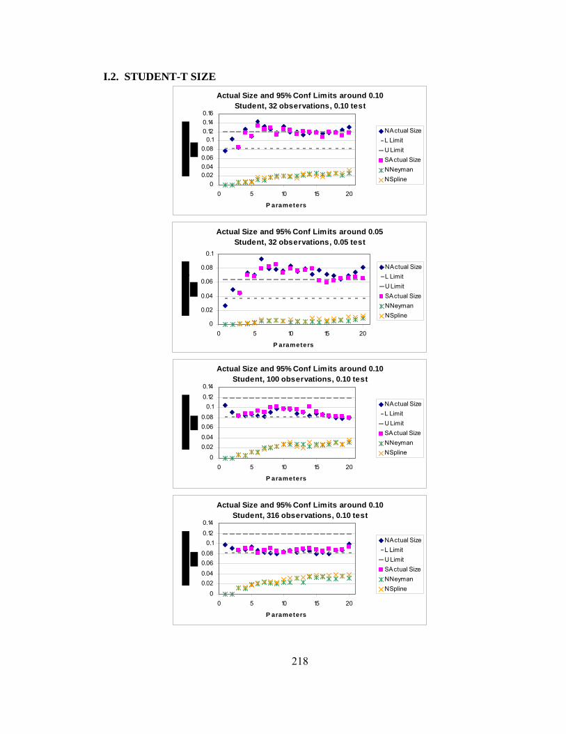
218

I.2. STUDENT-T SIZE Actual Size and 95% Conf Limits around 0.10

Student, 32 observations, 0.10 test

00.020.040.060.08

0.10.120.140.16

0 5 10 15 20

P arameters

NActual SizeL LimitU LimitSActual SizeNNeymanNSpline

Actual Size and 95% Conf Limits around 0.05

Student, 32 observations, 0.05 test

0

0.02

0.04

0.06

0.08

0.1

0 5 10 15 20

P arameters

NActual SizeL LimitU LimitSActual SizeNNeymanNSpline

Actual Size and 95% Conf Limits around 0.10

Student, 100 observations, 0.10 test

0

0.020.040.060.08

0.10.12

0.14

0 5 10 15 20

P arameters

NActual SizeL LimitU LimitSActual SizeNNeymanNSpline

Actual Size and 95% Conf Limits around 0.10

Student, 316 observations, 0.10 test

0

0.020.040.060.08

0.10.12

0.14

0 5 10 15 20

P arameters

NActual SizeL LimitU LimitSActual SizeNNeymanNSpline

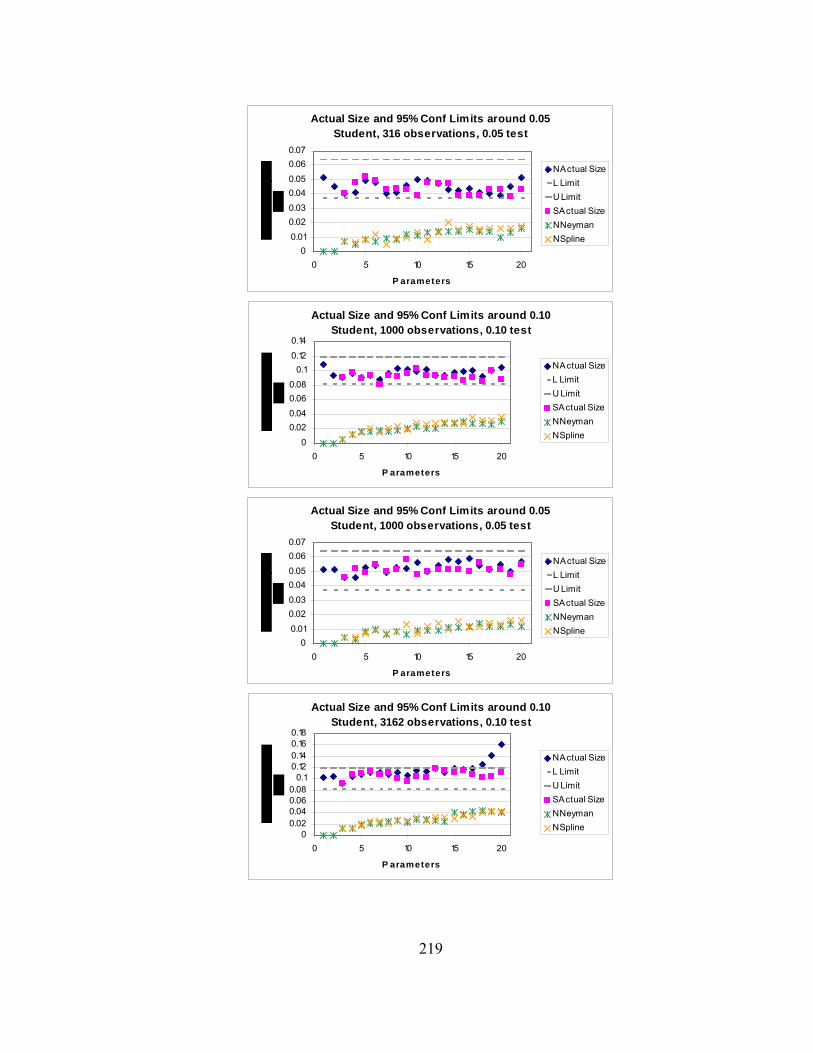
219

Actual Size and 95% Conf Limits around 0.05Student, 316 observations, 0.05 test

00.01

0.020.030.040.05

0.060.07

0 5 10 15 20

P arameters

NActual SizeL LimitU LimitSActual SizeNNeymanNSpline

Actual Size and 95% Conf Limits around 0.10

Student, 1000 observations, 0.10 test

0

0.020.040.060.08

0.10.12

0.14

0 5 10 15 20

P arameters

NActual SizeL LimitU LimitSActual SizeNNeymanNSpline

Actual Size and 95% Conf Limits around 0.05

Student, 1000 observations, 0.05 test

00.01

0.020.030.040.05

0.060.07

0 5 10 15 20

P arameters

NActual SizeL LimitU LimitSActual SizeNNeymanNSpline

Actual Size and 95% Conf Limits around 0.10

Student, 3162 observations, 0.10 test

00.020.040.060.08

0.10.120.140.160.18

0 5 10 15 20

P arameters

NActual SizeL LimitU LimitSActual SizeNNeymanNSpline

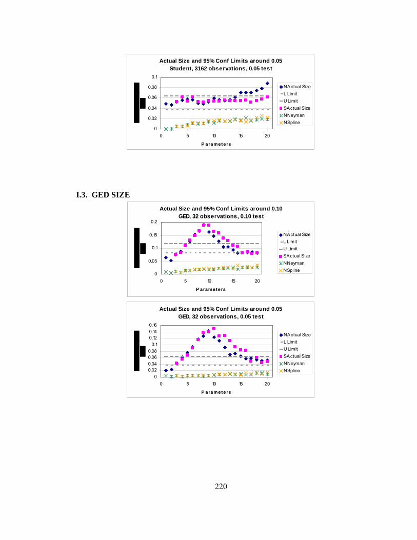
220

Actual Size and 95% Conf Limits around 0.05Student, 3162 observations, 0.05 test

0

0.02

0.04

0.06

0.08

0.1

0 5 10 15 20

P arameters

NActual SizeL LimitU LimitSActual SizeNNeymanNSpline

I.3. GED SIZE

Actual Size and 95% Conf Limits around 0.10GED, 32 observations, 0.10 test

0

0.05

0.1

0.15

0.2

0 5 10 15 20

P arameters

NActual SizeL LimitU LimitSActual SizeNNeymanNSpline

Actual Size and 95% Conf Limits around 0.05

GED, 32 observations, 0.05 test

00.020.040.060.08

0.10.120.140.16

0 5 10 15 20

P arameters

NActual SizeL LimitU LimitSActual SizeNNeymanNSpline

221

Actual Size and 95% Conf Limits around 0.10GED, 100 observations, 0.10 test

00.020.040.060.08

0.10.120.140.160.18

0 5 10 15 20

P arameters

NActual SizeL LimitU LimitSActual SizeNNeymanNSpline

Actual Size and 95% Conf Limits around 0.05

GED, 100 observations, 0.05 test

0

0.02

0.04

0.06

0.08

0.1

0.12

0 5 10 15 20

P arameters

NActual SizeL LimitU LimitSActual SizeNNeymanNSpline

Actual Size and 95% Conf Limits around 0.10

GED, 316 observations, 0.10 test

0

0.020.040.060.08

0.10.12

0.14

0 5 10 15 20

P arameters

NActual SizeL LimitU LimitSActual SizeNNeymanNSpline

Actual Size and 95% Conf Limits around 0.05

GED, 316 observations, 0.05 test

00.01

0.020.030.040.05

0.060.07

0 5 10 15 20

P arameters

NActual SizeL LimitU LimitSActual SizeNNeymanNSpline

222

Actual Size and 95% Conf Limits around 0.10GED, 1000 observations, 0.10 test

0

0.020.040.060.08

0.10.12

0.14

0 5 10 15 20

P arameters

NActual SizeL LimitU LimitSActual SizeNNeymanNSpline

Actual Size and 95% Conf Limits around 0.05GED, 1000 observations, 0.05 test

00.01

0.020.030.040.05

0.060.07

0 5 10 15 20

P arameters

NActual SizeL LimitU LimitSActual SizeNNeymanNSpline

Actual Size and 95% Conf Limits around 0.10

GED, 3162 observations, 0.10 test

0

0.020.040.060.08

0.10.12

0.14

0 5 10 15 20

P arameters

NActual SizeL LimitU LimitSActual SizeNNeymanNSpline

Actual Size and 95% Conf Limits around 0.05

GED, 3162 observations, 0.05 test

00.010.020.030.040.050.060.070.08

0 5 10 15 20

P arameters

NActual SizeL LimitU LimitSActual SizeNNeymanNSpline

223

I.4. MIXTURE SIZE Actual Size and 95% Conf Limits around 0.10

Mixture, 32 observations, 0.10 test

0

0.020.040.060.08

0.10.12

0.14

0 5 10 15 20

P arameters

NActual SizeL LimitU LimitSActual SizeNNeymanNSpline

Actual Size and 95% Conf Limits around 0.05

Mixture, 32 observations, 0.05 test

00.010.020.03

0.040.05

0.060.07

0 5 10 15 20

P arameters

NActual SizeL LimitU LimitSActual SizeNNeymanNSpline

Actual Size and 95% Conf Limits around 0.10

Mixture, 100 observations, 0.10 test

0

0.020.040.060.08

0.10.12

0.14

0 5 10 15 20

P arameters

NActual SizeL LimitU LimitSActual SizeNNeymanNSpline

Actual Size and 95% Conf Limits around 0.05

Mixture, 100 observations, 0.05 test

00.01

0.020.030.040.05

0.060.07

0 5 10 15 20

P arameters

NActual SizeL LimitU LimitSActual SizeNNeymanNSpline

224

Actual Size and 95% Conf Limits around 0.10Mixture, 316 observations, 0.10 test

0

0.020.040.060.08

0.10.12

0.14

0 5 10 15 20

P arameters

NActual SizeL LimitU LimitSActual SizeNNeymanNSpline

Actual Size and 95% Conf Limits around 0.05

Mixture, 316 observations, 0.05 test

00.01

0.020.030.040.05

0.060.07

0 5 10 15 20

P arameters

NActual SizeL LimitU LimitSActual SizeNNeymanNSpline

Actual Size and 95% Conf Limits around 0.10

Mixture, 1000 observations, 0.10 test

0

0.020.040.060.08

0.10.12

0.14

0 5 10 15 20

P arameters

NActual SizeL LimitU LimitSActual SizeNNeymanNSpline

Actual Size and 95% Conf Limits around 0.05

Mixture, 1000 observations, 0.05 test

00.01

0.020.030.040.05

0.060.07

0 5 10 15 20

P arameters

NActual SizeL LimitU LimitSActual SizeNNeymanNSpline

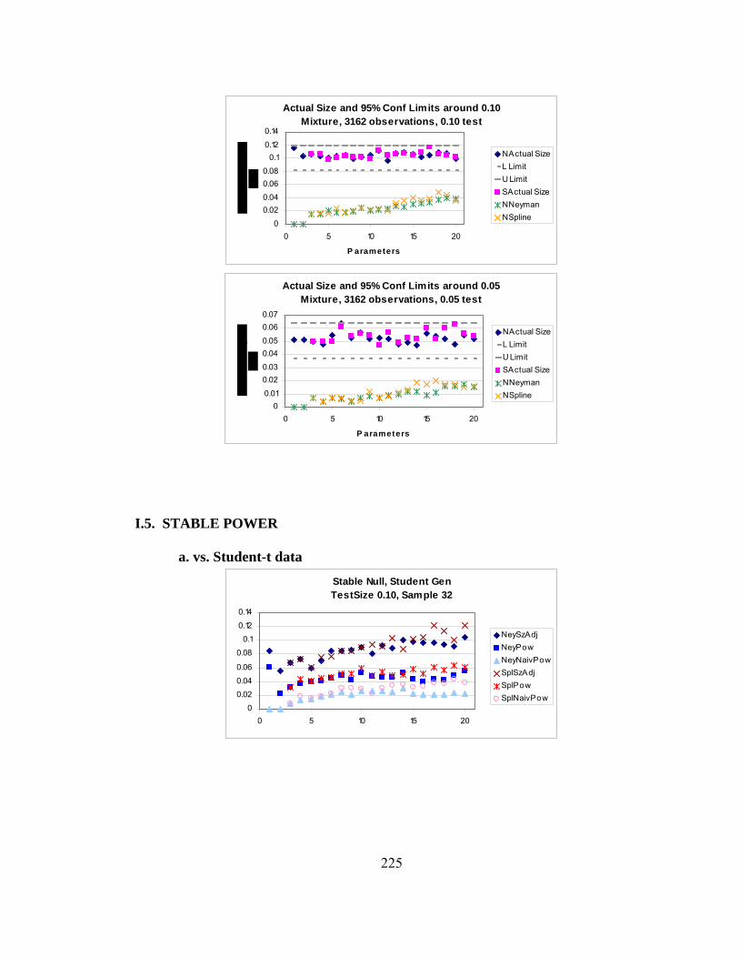
225

Actual Size and 95% Conf Limits around 0.10Mixture, 3162 observations, 0.10 test

0

0.020.040.060.08

0.10.12

0.14

0 5 10 15 20

P arameters

NActual SizeL LimitU LimitSActual SizeNNeymanNSpline

Actual Size and 95% Conf Limits around 0.05

Mixture, 3162 observations, 0.05 test

00.01

0.020.030.040.05

0.060.07

0 5 10 15 20

P arameters

NActual SizeL LimitU LimitSActual SizeNNeymanNSpline

I.5. STABLE POWER

a. vs. Student-t data Stable Null, Student GenTestSize 0.10, Sample 32

0

0.020.04

0.06

0.08

0.10.12

0.14

0 5 10 15 20

NeySzAdjNeyPowNeyNaivPowSplSzAdjSplPowSplNaivPow

226

Stable Null, Student GenTestSize 0.10, Sample 100

0

0.020.04

0.06

0.08

0.10.12

0.14

0 5 10 15 20

NeySzAdjNeyPowNeyNaivPowSplSzAdjSplPowSplNaivPow

Stable Null, Student GenTestSize 0.10, Sample 316

0

0.05

0.1

0.15

0.2

0.25

0 5 10 15 20

NeySzAdjNeyPowNeyNaivPowSplSzAdjSplPowSplNaivPow

Stable Null, Student GenTestSize 0.10, Sample 1000

0

0.1

0.2

0.3

0.4

0.5

0 5 10 15 20

NeySzAdjNeyPowNeyNaivPowSplSzAdjSplPowSplNaivPow

Stable Null, Student Gen

TestSize 0.10, Sample 3162

0

0.2

0.4

0.6

0.8

1

0 5 10 15 20

NeySzAdjNeyPowNeyNaivPowSplSzAdjSplPowSplNaivPow

b. vs. GED data

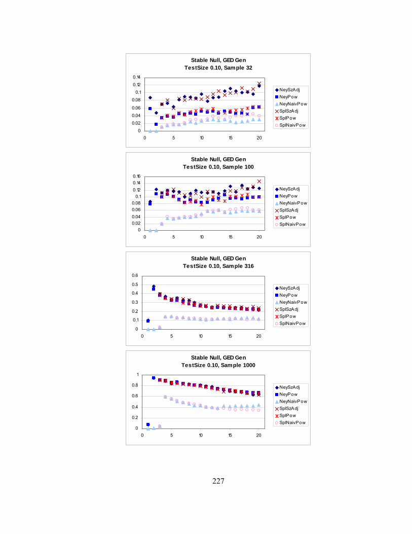
227

Stable Null, GED GenTestSize 0.10, Sample 32

0

0.020.04

0.06

0.08

0.10.12

0.14

0 5 10 15 20

NeySzAdjNeyPowNeyNaivPowSplSzAdjSplPowSplNaivPow

Stable Null, GED Gen

TestSize 0.10, Sample 100

00.020.040.060.08

0.10.120.140.16

0 5 10 15 20

NeySzAdjNeyPowNeyNaivPowSplSzAdjSplPowSplNaivPow

Stable Null, GED Gen

TestSize 0.10, Sample 316

0

0.1

0.2

0.3

0.4

0.5

0.6

0 5 10 15 20

NeySzAdjNeyPowNeyNaivPowSplSzAdjSplPowSplNaivPow

Stable Null, GED Gen

TestSize 0.10, Sample 1000

0

0.2

0.4

0.6

0.8

1

0 5 10 15 20

NeySzAdjNeyPowNeyNaivPowSplSzAdjSplPowSplNaivPow

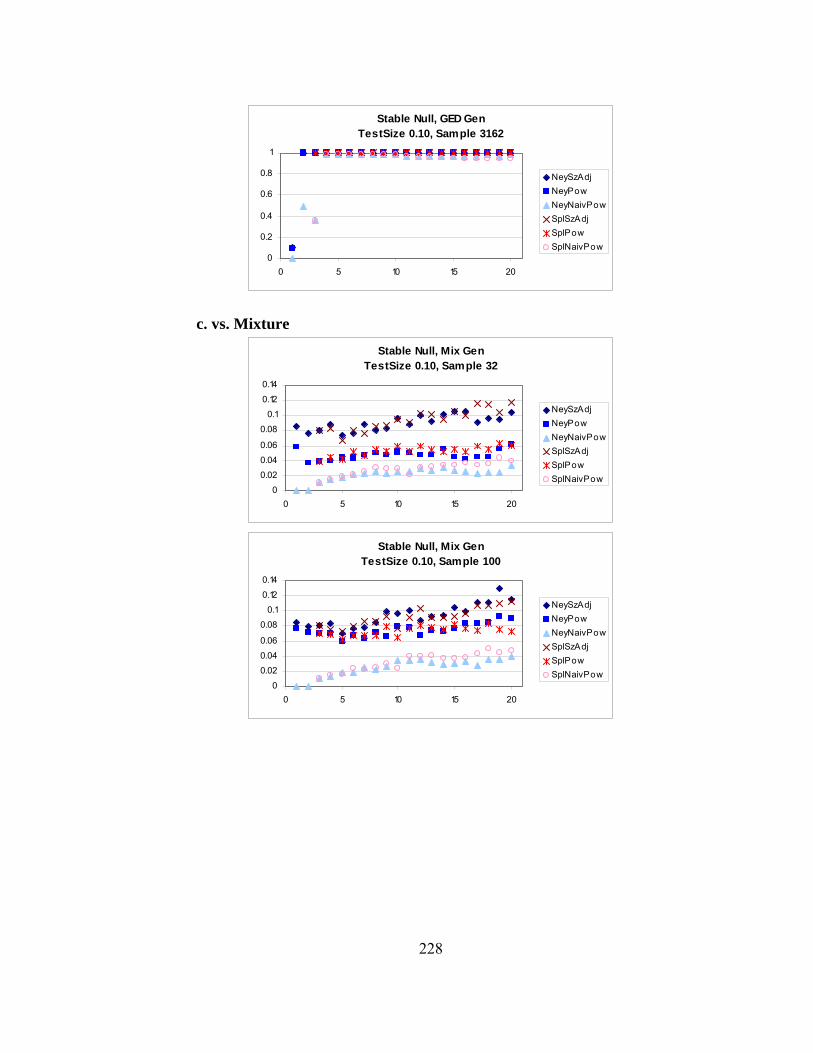
228

Stable Null, GED GenTestSize 0.10, Sample 3162

0

0.2

0.4

0.6

0.8

1

0 5 10 15 20

NeySzAdjNeyPowNeyNaivPowSplSzAdjSplPowSplNaivPow

c. vs. Mixture

Stable Null, Mix GenTestSize 0.10, Sample 32

0

0.020.04

0.06

0.08

0.10.12

0.14

0 5 10 15 20

NeySzAdjNeyPowNeyNaivPowSplSzAdjSplPowSplNaivPow

Stable Null, Mix Gen

TestSize 0.10, Sample 100

0

0.020.04

0.06

0.08

0.10.12

0.14

0 5 10 15 20

NeySzAdjNeyPowNeyNaivPowSplSzAdjSplPowSplNaivPow

229

Stable Null, Mix GenTestSize 0.10, Sample 316

0

0.02

0.04

0.06

0.08

0.1

0.12

0 5 10 15 20

NeySzAdjNeyPowNeyNaivPowSplSzAdjSplPowSplNaivPow

Stable Null, Mix Gen

TestSize 0.10, Sample 1000

00.020.040.060.08

0.10.120.140.16

0 5 10 15 20

NeySzAdjNeyPowNeyNaivPowSplSzAdjSplPowSplNaivPow

Stable Null, Mix Gen

TestSize 0.10, Sample 3162

00.05

0.10.150.2

0.250.3

0.350.4

0 5 10 15 20

NeySzAdjNeyPowNeyNaivPowSplSzAdjSplPowSplNaivPow

230

I.6. STUDENT-T POWER a. vs. Stable

Student Null, Stable GenTestSize 0.10, Sample 32

0

0.05

0.1

0.15

0.2

0.25

0 5 10 15 20

NeySzAdjNeyPowNeyNaivPowSplSzAdjSplPowSplNaivPow

Student Null, Stable Gen

TestSize 0.10, Sample 100

0

0.05

0.1

0.15

0.2

0.25

0.3

0 5 10 15 20

NeySzAdjNeyPowNeyNaivPowSplSzAdjSplPowSplNaivPow

Student Null, Stable Gen

TestSize 0.10, Sample 316

0

0.1

0.2

0.3

0.4

0.5

0.6

0 5 10 15 20

NeySzAdjNeyPowNeyNaivPowSplSzAdjSplPowSplNaivPow

231

Student Null, Stable GenTestSize 0.10, Sample 1000

00.10.20.30.40.50.60.70.80.9

0 5 10 15 20

NeySzAdjNeyPowNeyNaivPowSplSzAdjSplPowSplNaivPow

Student Null, Stable Gen

TestSize 0.10, Sample 3162

0

0.2

0.4

0.6

0.8

1

0 5 10 15 20

NeySzAdjNeyPowNeyNaivPowSplSzAdjSplPowSplNaivPow

b. vs. GED

232

Student Null, GED GenTestSize 0.10, Sample 32

0

0.020.04

0.06

0.08

0.10.12

0.14

0 5 10 15 20

NeySzAdjNeyPowNeyNaivPowSplSzAdjSplPowSplNaivPow

Student Null, GED Gen

TestSize 0.10, Sample 100

0

0.020.04

0.06

0.08

0.10.12

0.14

0 5 10 15 20

NeySzAdjNeyPowNeyNaivPowSplSzAdjSplPowSplNaivPow

Student Null, GED Gen

TestSize 0.10, Sample 316

0

0.05

0.1

0.15

0.2

0.25

0 5 10 15 20

NeySzAdjNeyPowNeyNaivPowSplSzAdjSplPowSplNaivPow

Student Null, GED Gen

TestSize 0.10, Sample 1000

0

0.1

0.2

0.3

0.4

0.5

0 5 10 15 20

NeySzAdjNeyPowNeyNaivPowSplSzAdjSplPowSplNaivPow

233

Student Null, GED GenTestSize 0.05, Sample 3162

0

0.2

0.4

0.6

0.8

1

0 5 10 15 20

NeySzAdjNeyPowNeyNaivPowSplSzAdjSplPowSplNaivPow

c. vs. Mixture Student Null, Mix Gen

TestSize 0.10, Sample 32

0

0.05

0.1

0.15

0.2

0 5 10 15 20

NeySzAdjNeyPowNeyNaivPowSplSzAdjSplPowSplNaivPow

Student Null, Mix Gen

TestSize 0.10, Sample 100

00.020.040.060.08

0.10.120.140.16

0 5 10 15 20

NeySzAdjNeyPowNeyNaivPowSplSzAdjSplPowSplNaivPow

Student Null, Mix Gen

TestSize 0.10, Sample 316

0

0.05

0.1

0.15

0.2

0.25

0 5 10 15 20

NeySzAdjNeyPowNeyNaivPowSplSzAdjSplPowSplNaivPow

234

Student Null, Mix GenTestSize 0.10, Sample 1000

00.05

0.10.150.2

0.250.3

0.350.4

0 5 10 15 20

NeySzAdjNeyPowNeyNaivPowSplSzAdjSplPowSplNaivPow

Student Null, Mix Gen

TestSize 0.10, Sample 3162

00.10.20.30.40.50.60.70.8

0 5 10 15 20

NeySzAdjNeyPowNeyNaivPowSplSzAdjSplPowSplNaivPow

I.7. GED POWER a. vs. Stable

GED Null, Stable GenTestSize 0.10, Sample 32

0

0.05

0.1

0.15

0.2

0.25

0.3

0 5 10 15 20

NeySzAdjNeyPowNeyNaivPowSplSzAdjSplPowSplNaivPow

235

GED Null, Stable GenTestSize 0.10, Sample 100

00.05

0.10.150.2

0.250.3

0.350.4

0.45

0 5 10 15 20

NeySzAdjNeyPowNeyNaivPowSplSzAdjSplPowSplNaivPow

GED Null, Stable Gen

TestSize 0.10, Sample 316

00.10.20.30.40.50.60.70.80.9

0 5 10 15 20

NeySzAdjNeyPowNeyNaivPowSplSzAdjSplPowSplNaivPow

GED Null, Stable Gen

TestSize 0.10, Sample 1000

0

0.2

0.4

0.6

0.8

1

0 5 10 15 20

NeySzAdjNeyPowNeyNaivPowSplSzAdjSplPowSplNaivPow

GED Null, Stable Gen

TestSize 0.10, Sample 3162

0

0.2

0.4

0.6

0.8

1

0 5 10 15 20

NeySzAdjNeyPowNeyNaivPowSplSzAdjSplPowSplNaivPow

236

b. vs. Student-t

GED Null, Student GenTestSize 0.10, Sample 32

0

0.05

0.1

0.15

0.2

0.25

0 5 10 15 20

NeySzAdjNeyPowNeyNaivPowSplSzAdjSplPowSplNaivPow

GED Null, Student Gen

TestSize 0.10, Sample 100

0

0.05

0.1

0.15

0.2

0.25

0 5 10 15 20

NeySzAdjNeyPowNeyNaivPowSplSzAdjSplPowSplNaivPow

GED Null, Student Gen

TestSize 0.10, Sample 316

0

0.05

0.1

0.15

0.2

0.25

0.3

0 5 10 15 20

NeySzAdjNeyPowNeyNaivPowSplSzAdjSplPowSplNaivPow

GED Null, Student Gen

TestSize 0.10, Sample 1000

0

0.10.2

0.3

0.4

0.50.6

0.7

0 5 10 15 20

NeySzAdjNeyPowNeyNaivPowSplSzAdjSplPowSplNaivPow

237

GED Null, Student GenTestSize 0.10, Sample 3162

0

0.2

0.4

0.6

0.8

1

0 5 10 15 20

NeySzAdjNeyPowNeyNaivPowSplSzAdjSplPowSplNaivPow

c. vs. Mixture GED Null, Mix Gen

TestSize 0.10, Sample 32

0

0.05

0.1

0.15

0.2

0.25

0 5 10 15 20

NeySzAdjNeyPowNeyNaivPowSplSzAdjSplPowSplNaivPow

GED Null, Mix Gen

TestSize 0.10, Sample 100

0

0.050.1

0.15

0.2

0.250.3

0.35

0 5 10 15 20

NeySzAdjNeyPowNeyNaivPowSplSzAdjSplPowSplNaivPow

GED Null, Mix Gen

TestSize 0.10, Sample 316

0

0.1

0.2

0.3

0.4

0.5

0.6

0 5 10 15 20

NeySzAdjNeyPowNeyNaivPowSplSzAdjSplPowSplNaivPow

238

GED Null, Mix GenTestSize 0.10, Sample 1000

0

0.2

0.4

0.6

0.8

1

0 5 10 15 20

NeySzAdjNeyPowNeyNaivPowSplSzAdjSplPowSplNaivPow

GED Null, Mix Gen

TestSize 0.10, Sample 3162

0

0.2

0.4

0.6

0.8

1

0 5 10 15 20

NeySzAdjNeyPowNeyNaivPowSplSzAdjSplPowSplNaivPow

I.8. MIXTURE POWER a. vs. Stable

Mixture Null, Stable GenTestSize 0.10, Sample 32

0

0.020.04

0.06

0.08

0.10.12

0.14

0 5 10 15 20

NeySzAdjNeyPowNeyNaivPowSplSzAdjSplPowSplNaivPow

239

Mixture Null, Stable GenTestSize 0.10, Sample 100

0

0.020.04

0.06

0.08

0.10.12

0.14

0 5 10 15 20

NeySzAdjNeyPowNeyNaivPowSplSzAdjSplPowSplNaivPow

Mixture Null, Stable Gen

TestSize 0.10, Sample 316

00.020.040.060.08

0.10.120.140.160.18

0 5 10 15 20

NeySzAdjNeyPowNeyNaivPowSplSzAdjSplPowSplNaivPow

Mixture Null, Stable Gen

TestSize 0.05, Sample 1000

0

0.05

0.1

0.15

0.2

0.25

0 5 10 15 20

NeySzAdjNeyPowNeyNaivPowSplSzAdjSplPowSplNaivPow

Mixture Null, Stable Gen

TestSize 0.10, Sample 3162

00.10.20.30.40.50.60.70.80.9

0 5 10 15 20

NeySzAdjNeyPowNeyNaivPowSplSzAdjSplPowSplNaivPow

240

b. vs. Student-t

Mixture Null, Student GenTestSize 0.10, Sample 32

0

0.02

0.04

0.06

0.08

0.1

0.12

0 5 10 15 20

NeySzAdjNeyPowNeyNaivPowSplSzAdjSplPowSplNaivPow

Mixture Null, Student GenTestSize 0.10, Sample 100

0

0.02

0.04

0.06

0.08

0.1

0.12

0 5 10 15 20

NeySzAdjNeyPowNeyNaivPowSplSzAdjSplPowSplNaivPow

Mixture Null, Student GenTestSize 0.10, Sample 316

0

0.020.04

0.06

0.08

0.10.12

0.14

0 5 10 15 20

NeySzAdjNeyPowNeyNaivPowSplSzAdjSplPowSplNaivPow

Mixture Null, Student Gen

TestSize 0.10, Sample 1000

0

0.05

0.1

0.15

0.2

0.25

0 5 10 15 20

NeySzAdjNeyPowNeyNaivPowSplSzAdjSplPowSplNaivPow

241

Mixture Null, Student GenTestSize 0.10, Sample 3162

0

0.1

0.2

0.3

0.4

0.5

0 5 10 15 20

NeySzAdjNeyPowNeyNaivPowSplSzAdjSplPowSplNaivPow

c. vs. GED Mixture Null, GED Gen

TestSize 0.10, Sample 32

0

0.02

0.04

0.06

0.08

0.1

0.12

0 5 10 15 20

NeySzAdjNeyPowNeyNaivPowSplSzAdjSplPowSplNaivPow

Mixture Null, GED Gen

TestSize 0.10, Sample 100

0

0.02

0.04

0.06

0.08

0.1

0.12

0 5 10 15 20

NeySzAdjNeyPowNeyNaivPowSplSzAdjSplPowSplNaivPow

Mixture Null, GED Gen

TestSize 0.10, Sample 316

0

0.020.04

0.06

0.08

0.10.12

0.14

0 5 10 15 20

NeySzAdjNeyPowNeyNaivPowSplSzAdjSplPowSplNaivPow

242

Mixture Null, GED GenTestSize 0.10, Sample 1000

0

0.05

0.1

0.15

0.2

0.25

0.3

0 5 10 15 20

NeySzAdjNeyPowNeyNaivPowSplSzAdjSplPowSplNaivPow

Mixture Null, GED Gen

TestSize 0.10, Sample 3162

0

0.10.2

0.3

0.4

0.50.6

0.7

0 5 10 15 20

NeySzAdjNeyPowNeyNaivPowSplSzAdjSplPowSplNaivPow

243

BIBLIOGRAPHY

Adler, Robert J., Raisa E. Feldman, and Murad S. Taqqu, Editors, A Practical Guide to Heavy Tails, Birkhäuser, 1998.

Andrews, Donald W.K., “A Conditional Kolmogorov Test,” Econometrica, 65, 1097-1128, 1997.

Bai, Jushan, “Testing Parametric Conditional Distributions of Dynamic Models,” MIT Department of Economics, 1997.

Bera, Anil K. and Colin R. McKenzie, “Tests for Normal with Stable Alternatives,” Journal of Statistical Computation and Simulation, 25, 37-52, 1986.

Blattberg, R. and N. Gonedes, 1974, "A Comparison of the Stable and Student Distributions as Statistical Models for Stock Prices," Journal of Business 47, 244-280.

Bollerslev, T., “A Conditional Heteroskedastic Time Series Model for Speculative Prices and Rates of Return,” Review of Economics and Statistics, 69, 542-547, 1987. Boothe, Paul, and Debra Glassman, “The Statistical Distribution of Exchange Rates,” Journal of International Economics, 22, 297-319, 1987. Borak, Szymon, Wolgang Härdle, Rafal Waron, “Stable Distributions,” SFB Discussion Paper 2005-008. Borowski, E.J., and Borwein, J.M., The HarperCollins Dictionary of Mathematics, HarperPerennial, 1991. Box, George E.P. and Gwilym M Jenkins, Time Series Analysis: Forecasting and Control, Holden-Day, 1970. Campbell, JohnY., AndrewW. Lo, and A.Craig MacKinlay, The Econometrics of Financial Markets, Princeton University Press, 1997. Chernoff, H. and E.L. Lehmann, “The Use of Maximum Likelihood Estiamtes in χ2 Tests for Goodness of Fit,” Ann. Math. Statist., 25, 579-586, 1954. Clark, Peter K., “A Subordinated Stochastic Process Model with Finite Variance for Speculative Prices,” Econometrica, 41, 135-155, 1973.

244

Davidson, Russell, and James G. MacKinnon, Estimation and Inference in Econometrics, Oxford University Press, 1993. DeGroot, Morris, Probability and Statistics, Second Edition, Addison-Wesley, 1986. Engle, R., and G. Gonzalez-Rivera, 1991, “Semiparametric ARCH Models,” Journal of Business and Economic Statistics, 9, 345-359, 1991.

Fama, E., 1965, "The Behavior of Stock Prices," Journal of Business 38, 34-105.

Fama, E., 1976, Foundations of Finance. New York: Basic Books.

Fama, Eugene F., and Kenneth R. French, “Dividend Yields and Expected Stock Returns,” Journal of Financial Economics, 22, 3-25, 1988. Fama, Eugene F., and Kenneth R. French, “Business Conditions and Expected Returns on Stocks and Bonds,” Journal of Financial Economics, 25, 23-49, 1989. French, Kenneth R., http://mba.tuck.dartmouth.edu/pages/faculty/ken.french/data_library.html, October 2003 Hagerman, Robert L., “More Evidence on the Distribution of Security Returns,” Journal of Finance, 33, pp. 1213-1221, 1978. Hogg, Robert V., and Allen T. Craig, Introduction to Mathematical Statistics, Third Edition, MacMillan Publishing Company, 1970. Judd, Kenneth L., Numerical Methods in Economics, The MIT Press, 1999. Kellison, Stephen G., Fundamentals of Numerical Analysis, Richard D. Irwin, Inc., 1975 Li, Qi, “Semiparametric Estimation and Testing of Econometric Models,” Department of Economics, University of Guelph (Canada), 1997. Mandelbrot, Benoit, “ The Variation of Certain Speculative Prices,” Journal of Business, 36, 394-419, 1963. Marsaglia, G. (2000) “The Monster, A Random Number Generator with Period over 102857 Times as Long as the Previously Touted Longest-period One,” noted at http://www.aptech.com/random McCulloch, J. Huston, “Simple Consistent Estimators of Stable Distribution Parameters,” Communications in Statistics—Simulation, 15, 1109-1136.

245

McCulloch, J. Huston, "Numerical Approximation of the Symmetric Stable Distribution and Density," OSU Econ Dept., Oct. 1994. McCulloch, J. Huston, “Measuring the Term Structure of Interest Rates,” Journal of Business, 44, 19-31, 1971. McCulloch, J. Huston, “The Tax-Adjusted Yield Curve,” Journal of Finance, 20, 811-30, 1975. McCulloch, J. Huston, “Financial Applications of Stable Distributions,” Statistical Methods in Finance (Handbook of Statistics 14), G.S. Maddala and C.R.Rao, eds., Elsevier Science, Amsterdam, 1996. McCulloch, J. Huston, “Measuring Tail Thickness to Estimate the Stable Index α: A Critique,” Journal of Business & Economic Statistics, Vol. 15, No. 1, 74-81, January 1997. McCulloch, J. Huston, "Linear Regression with Stable Disturbances," in R. Adler, R. Feldman, and M.S. Taqqu, eds., A Practical Guide to Heavy Tails, Birkhaeuser, Boston, 1998. McCulloch, J. Huston, “A Spline Rao Score (LM) Test for Goodness of Fit: A Proposal,” 1999. Mood, Alexander M., Franklin A. Graybill, and Duane C. Boes, Introduction to the Theory of Statistics, Third Edition, McGraw-Hill, 1974. Nelson, D., “Conditional Heteroskedasticity in Asset Returns: A New Approach,” Econometrica, 59, 347-370, 1991. Pagan, Adrian, and Aman Ullah, Nonparametric Econometrics, Cambridge University Press, 1999. Perry, Philip R., “More Evidence on the Nature of the Distribution of Security Returns,” Journal of Financial and Quantitative Analysis, 18, 211-221, 1983. Praetz, Peter D., “The Distribution of Share Price Changes,” Journal of Business, 45, 49-55, 1972. Press, William H., Saul A. Teukolsky, William T. Vetterling, Brian P. Flannery, Numerical Recipes in Fortran 77: The Art of Scientific Computing, Second Edition, Cambridge University Press, 1992.

246

Ralston, Anthony and Philip Rabinowitz, A First Course in Numerical Analysis, Dover Publications, Inc., 1978 Rayner, J.C.W., and D.J. Best, Smooth Tests of Goodness of Fit, Oxford University Press, 1989. Salsburg, David, The Lady Tasting Tea: How Statistics Revolutionized Science in the Twentieth Century, Henry Holt and Company, 2001. Samorodnitsky, Gennady, and Murad S. Taqqu, Stable Non-Gaussian Random Processes: Stochastic Processes with Infinite Variance,” Chapman and Hall, New York, 1994. Taylor, S., Modeling Financial Time Series, London: John Wiley & Sons, 1986. Wilkinson, J. H., Rounding Errors in Algebraic Processes, Prentice-Hall, Inc., 1963.