a continuum thermodynamics formulation for micro-magneto ...landis/landis/research... · a...

ARTICLE IN PRESS

Contents lists available at ScienceDirect

Journal of the Mechanics and Physics of Solids

Journal of the Mechanics and Physics of Solids 56 (2008) 3059– 3076

0022-50

doi:10.1

� Tel.

E-m

journal homepage: www.elsevier.com/locate/jmps

A continuum thermodynamics formulation for micro-magneto-mechanics with applications to ferromagnetic shape memory alloys

Chad M. Landis �

Department of Aerospace Engineering and Engineering Mechanics, The University of Texas at Austin, 210 East 24th Street, C0600, Austin, TX 78712-0235, USA

a r t i c l e i n f o

Article history:

Received 2 October 2007

Received in revised form

22 April 2008

Accepted 26 May 2008

Keywords:

Phase transformation

Twinning

Constitutive behavior

Ferromagnetic shape memory material

Sensors and actuators

96/$ - see front matter & 2008 Elsevier Ltd. A

016/j.jmps.2008.05.004

: +1512 4714273; fax: +1512 4715500.

ail address: [email protected]

a b s t r a c t

A continuum thermodynamics formulation for micromagnetics coupled with mechanics is

devised to model the evolution of magnetic domain and martensite twin structures in

ferromagnetic shape memory alloys. The theory falls into the class of phase-field or diffuse-

interface modeling approaches. In addition to the standard mechanical and magnetic

balance laws, two sets of micro-forces and their associated balance laws are postulated; one

set for the magnetization order parameter and one set for the martensite order parameter.

Next, the second law of thermodynamics is analyzed to identify the appropriate material

constitutive relationships. The proposed formulation does not constrain the magnitude of

the magnetization to be constant, allowing for spontaneous magnetization changes

associated with strain and temperature. The equations governing the evolution of the

magnetization are shown to reduce to the commonly accepted Landau–Lifshitz–Gilbert

equations for the case where the magnetization magnitude is constant. Furthermore, the

analysis demonstrates that under certain limiting conditions, the equations governing the

evolution of the martensite-free strain are shown to be equivalent to a hyperelastic strain

gradient theory. Finally, numerical solutions are presented to investigate the fundamental

interactions between the magnetic domain wall and the martensite twin boundary in

ferromagnetic shape memory alloys. These calculations determine under what conditions

the magnetic domain wall and the martensite twin boundary can be dissociated, resulting

in a limit to the actuating strength of the material.

& 2008 Elsevier Ltd. All rights reserved.

1. Introduction

Ferromagnetic shape memory alloys (FSMAs) are materials with very strong magnetic and mechanical coupling. Forexample, in nickel–magnesium–gallium (NiMnGa) alloys applied magnetic fields can cause actuation strains on the orderof 6–10% (Tickle and James, 1999; Tickle, 2000; Murray et al., 2001; Sozinov et al., 2002), while other magnetostrictivematerials of interest like terfenol and galfenol can provide strains at not even one-tenth of this level. The large strain inNiMnGa is due to the coupling between the mechanical twin structure and the magnetic domain structure (James andWuttig, 1998; O’Handley et al., 2000; Kiefer and Lagoudas, 2005; Ma and Li, 2007a, b). Below the Curie temperature,NiMnGa has a tetragonal crystal structure with the c-axis shorter than the a-axes. The material is also ferromagnetic withits easy axis of magnetization aligned with the c-axis. As in all martensitic and ferromagnetic materials, domain structuresare formed that tend to minimize the energies associated with elastic and magnetic interactions, stray fields, and domainwall and twin boundary surface energies. When the magnetocrystalline anisotropy energy is high, the magnetic domain

ll rights reserved.

www.sciencedirect.com/science/journal/mps

www.elsevier.com/locate/jmps

dx.doi.org/10.1016/j.jmps.2008.05.004

mailto:[email protected]

ARTICLE IN PRESS

C.M. Landis / J. Mech. Phys. Solids 56 (2008) 3059–30763060

walls and martensite twin boundaries lie on top of one another and tend to move through the crystal in concert. Suchcooperative defect motions furnish the material with the potential to deliver large actuating strains through the applicationof a magnetic field. However, these strains are significantly smaller in the presence of a blocking stress. Specifically,experimental investigations on NiMnGa materials have shown that practically no actuating strains exist even for largelevels of applied magnetic field if the material is under a 2–5 MPa compressive stress (Karaca et al., 2006). Hence, eventhough large stress-free strains can be obtained from FSMAs, these materials are not able to supply much actuation energy

due to the relatively low blocking stress (Kiefer et al., 2007).This paper presents a theoretical approach to describe magnetic domain walls, martensite twin boundaries, and their

nonlinear interactions. The approach differs from ‘‘constrained’’ approaches (DeSimone and James, 1997, 2002; Ma and Li,2007a) where the evolution of energy minimizing laminate domain structures are studied, and the detailed structure andbehavior of the domain walls is not considered. Instead, the theory falls into the class of ‘‘phase-field’’ or ‘‘diffuse interface’’theories, wherein the material interfaces have a well-defined thickness (Chen, 2002). The approach reduces to the acceptedLandau–Lifshitz–Gilbert (LLG) equations for the micromagnetic response, and to the Landau–Ginzburg phase-fieldequations for the ‘‘microelastic’’ response. Unlike traditional methods for deriving the governing phase-field equations,which rely on energy minimization concepts, this paper applies a continuum thermodynamics approach. Specifically, thetheory postulates the existence of micro-forces that are work conjugate to the martensite and magnetic order parameters,and the associated balance laws for these micro-forces. Thereafter, the second law of thermodynamics is analyzed to obtainthe appropriate constitutive equations and restrictions on the dissipation.

To apply the theory to a material class of interest, a material-free energy is selected to mimic the behavior of FSMAs. Thegoverning micro-magneto-mechanical equations are solved to determine the magnetic domain wall and martensite twinboundary structures. An analysis of the energetic forces that cause motion of these defects is also given. Finally, it ishypothesized that the mechanism for the low blocking stress levels in these materials is the dissociation of the martensitetwin boundaries from the 901 magnetic domain walls. The model is used to predict several features of this behaviorincluding the critical stress required to tear the martensite twin from the magnetic domain wall. The calculations areshown to predict blocking stress levels similar to those found experimentally.

2. Theory

Traditionally, the micromagnetics equations governing the evolution of domain configurations have been derived from asimple and physically justifiable set of assumptions (Landau and Lifsitz, 1935; Gilbert, 1956, 2004; Brown, 1963). While thisapproach is certainly sound, it obscures the continuum physics distinction between fundamental balance laws, which areapplicable to a wide range of materials, and the constitutive equations that are valid for a specific material (Fried andGurtin, 1993, 1994; Gurtin, 1996). Here a small deformation non-equilibrium thermodynamics framework forferromagnetic domain and martensite twin evolution is presented. The fundamental equations governing the magneto-mechanical fields under the assumption of small deformations and rotations are used as the starting point. Note that thesmall deformation assumption is prevalent throughout the micromagnetic modeling literature. The analysis of largedeformations would introduce the concept of Maxwell stresses, which are here assumed to be higher order effects that canbe neglected. Following previous micromagnetic modeling approaches, e.g. Zhang and Chen (2005a, b), the effects of largedeformations will not be considered, but their incorporation within the theory is possible. It will also be assumed that thefields vary slowly in time with respect to any electromagnetic fluctuations in the material, yielding the quasi-staticelectromagnetic field approximation, but not necessarily with respect to the speed of sound, allowing for inertial effects tobe considered within the general derivation. Under these assumptions, the balances of linear and angular momentum inany arbitrary volume V and its bounding surfaces S yield:

sji;j þ bi ¼ r €ui in V , (2.1)

sij ¼ sji in V , (2.2)

sjinj ¼ ti on S, (2.3)

where sij are the Cartesian components of the Cauchy stress, bi are the components of a body force per unit volume, r is themass density, ui are the mechanical displacements, ni are the components of a unit vector normal to a surface element, andti are the tractions applied to the surface. Standard index notation is used with summation implied over repeated indices,the double overdot represents a second derivative with respect to time, and ,j represents partial differentiation with respectto the xj coordinate direction. Under the assumptions of linear kinematics, the strain components eij are related to thedisplacements as:

�ij ¼12ðui;j þ uj;iÞ in V . (2.4)

The magnetic field, Hi, magnetic induction, Bi, volume current density, Ji, surface current density, Ki, and the magneticvector potential, Ai, are governed by the quasi-static forms of Maxwell’s equations. Specifically, in any arbitrary volume V

ARTICLE IN PRESS

C.M. Landis / J. Mech. Phys. Solids 56 (2008) 3059–3076 3061

(including a region of free space) and its bounding surface S:

Bi;i ¼ 0) Bi ¼ EijkAk;j in V , (2.5)

EijkHk;j ¼ Ji in V , (2.6)

EijkHjnk ¼ Ki on S, (2.7)

where Eijk is the permutation tensor such that Eijk ¼ 1 if ijk ¼ 123, 231, or 312, Eijk ¼ �1 if ijk ¼ 321, 132, or 213, and Eijk ¼ 0for all other combinations of ijk. Within the theory of small deformation magnetostriction, Eqs. (2.1)–(2.7) represent thefundamental balance laws and kinematic relationships, and the constitutive laws required to close the loop on theequations relate the stress and magnetic field to the strain and magnetic induction. Such constitutive relationships can bederived from thermodynamic considerations using a material-free energy that depends on the components of the strainand magnetic induction (Nye, 1957). However, within the micro-magneto-mechanical modeling approach derived here thefree energy will also be required to depend on the magnetization and its gradient, and on the martensite-free strain and itsgradient. Note that the relationship between magnetic field, magnetic induction and material magnetization is given as:

Bi ¼ m0ðHi þMiÞ in V . (2.8)

Here m0 is the permittivity of free space. Given that the free energy will be allowed to depend on an additionalindependent variable Mi, we must now allow for a new system of ‘‘micro-forces’’ that are work conjugate to thisconfigurational quantity. Following the work of Fried and Gurtin (1993, 1994), we introduce a micro-force tensor xji suchthat xjinj

_Mi represents a power density expended across surfaces by neighboring configurations, an internal micro-forcevector pi such that pi

_Mi is the power density expended by the material internally, e.g. in the ordering of spin within thelattice (this micro-force will account for dissipation in the material), and an external micro-force vector fi such that f i

_Mi is apower density expended on the material by external sources. In micromagnetics, the fundamental balance law relates themagnetic torque to the rate of change of the angular momentum (Landau and Lifsitz, 1935). In the present continuumframework, for an arbitrary volume of material, this angular momentum balance takes the following form:

1

m0

ZSEijkMjxlinl dSþ

ZVEijkMjpk dV þ

ZVEijkMjf k dV

� �¼

ZV

1

g0

_Mi dV . (2.9)

Here g0 ¼ �gjejm0=ð2mÞ ¼ �2:214� 105 m=ðA sÞ is the gyromagnetic ratio for an electron spin, although within thisphenomenological framework g0 can be used as a free parameter. In Eq. (2.9), the left-hand side is the torque associatedwith the moment of the micro-forces and the magnetization, and the right-hand side is the rate of change of the angularmomentum associated with the changes in the magnetization. Application of the divergence theorem to the first term, andrecognizing that this balance law must hold for any arbitrary volume, yields the following point-wise balance law:

EkjiMjðxli;l þ pi þ f iÞ þ EkjiMj;lxli ¼m0

g0

_Mk. (2.10)

Eq. (2.10) will be shown to lead to the Landau–Lifshitz–Gilbert equation of micromagnetics after the analysis of thesecond law of thermodynamics is performed. Taking the cross product of Eq. (2.10) with the magnetization leads to:

M2ðxli;l þ pi þ f iÞ �MiMjðxlj;l þ pj þ f jÞ þ EijkEjrsMr;lxlsMk ¼ Eijk

m0

g0

_MjMk. (2.11)

Eq. (2.11) gives no information on how the micro-forces affect the rate of change of the magnetization parallel to itsdirection, i.e. the change in its magnitude. Therefore, it will be assumed that the micro-forces in the direction of themagnetization are always in equilibrium. This assumption implies that the changes in magnetization magnitude occur suchthat a micro-force balance along the magnetization direction holds at every instant in time. Physically, such changes inmagnitude are not instantaneous. However, it is assumed that these changes occur on much shorter time scales than thoseassociated with the rotation of the magnetization. Mathematically, this balance condition is stated as:

Mjðxlj;l þ pj þ f jÞ ¼ 0. (2.12)

Then, applying this assumption within Eq. (2.11) yields the following equation for the micro-forces:

xli;l þ pi þ f i ¼ Eijkm0

g0M2_MjMk �

EijkEjrs

M2Mr;lxlsMk. (2.13)

Eq. (2.13) is ultimately a continuum statement of the conservation of angular momentum associated with the electronicspin and the balance of micro-forces in the direction of the magnetization. This equation will eventually be used to developfinite element formulations for numerical solutions of the coupled magneto-mechanical equations.

In the literature on ferroelectric materials, the use of the polarization vector as the sole order parameter is prevalent andleads to a reasonable description of domain wall structures and domain wall surface energies (Su and Landis, 2007).However, we have found that the same assumption for FSMAs, i.e. employing the magnetization as the sole orderparameter, leads to a somewhat unrealistic domain wall structure and domain wall energy. The difficulty arises in thedescription of the strain, which must be quadratic in the magnetization. The strain change between different martensite

landis

Sticky Note

Typo - Free index on this term should be k not i.

ARTICLE IN PRESS


variants in NiMnGa alloys is in the range of 6%, and with elastic properties on the order of 100 GPa, this leads to stresseswithin the domain walls of about 6 GPa. This relatively large stress state results in ‘‘thinning’’ of the domain walls in orderto compensate for this large strain energy and reduce the overall energy of the wall. Consequently, it is expected that amore realistic description of FSMAs would incorporate a second strain-like order parameter in order to describe themartensite twin boundaries. In this paper, a second-rank tensor order parameter with components �0

ij is introduced, and isused to describe the possible martensite variants. This quantity is referred to as the free-strain, and it is distinct from thespontaneous strain since it is not a constant valued tensor. Specifically, considering only spatially homogenous states,the spontaneous strain is defined to be the strain state at zero stress, zero micro-force and zero magnetic field. Whereas,the free-strain is the strain state at zero stress but not necessarily zero micro-force and magnetic field. Again, we introducea system of micro-forces, zkjink (surface), Wji (internal), and gji (external), which do work on changes in �0

ij. Additionally, abalance of these micro-forces is assumed such thatZ

Szkjink dSþ

ZVWji dV þ

ZV

gji dV ¼ 0, (2.14)

which implies the point-wise balance:

zkji;k þ Wji þ gji ¼ 0. (2.15)

To remain as general as possible, it is assumed that the Helmholtz-free energy of the material (including the free spaceoccupied by the material) takes the following form:

C ¼ Cð�ij;Bi;Mi;Mi;j; _Mi; �0ij; �

0ij;k; _�

0ijÞ. (2.16)

Note that temperature plays a key role in magnetic and martensitic phase transitions near the Curie point or theaustenite to martensite transition temperature. Near the Curie temperature, changes in the magnetization magnitude areparticularly important. For spatially homogeneous isothermal behavior, the Helmholtz-free energy remains the appropriateenergy functional with the additional complication that the material parameters of the free energy are temperaturedependent. Here we will deal only with constant temperature behavior below the two transition temperatures, butrecognize that the extension to spatially homogeneous temperature dependent behavior can be readily included within thepresent framework simply by specifying the temperature at which the material properties must be evaluated at eachinstant in time. In contrast, the inclusion of spatially inhomogeneous temperature-dependent behavior, and the associatedthermal diffusion, requires an analysis of the second law of thermodynamics including such effects. In such cases, thetemperature and entropy must be introduced as additional field variables within the theory and the numerical treatment.In this paper, only constant temperature cases will be considered.

For the isothermal processes below the transition temperatures under consideration, the second law ofthermodynamics is written as the Clausius–Duhem (dissipation) inequality as:Z

V

_CdV þd

dt

ZV

1

2r _ui _ui dVp

ZVðbi _ui þ Ji

_Ai þ f i_Mi þ gji _�

0ijÞdV þ

ZSðti _ui þ Ki

_Ai þ xjinj_Mi þ zkjink _�

0ijÞdS. (2.17)

The left-hand side of this inequality represents the rate of change of the stored plus kinetic energy of the material (andfree space). The right-hand side represents the work rates due to externally applied mechanical forces, steady currents, andmicro-forces. Note that the internal micro-forces pi and Wji do not contribute to the external power. The difference betweenthe right- and left-hand sides of the equation is simply the dissipation, and the inequality specifies that the dissipationmust be non-negative. Analysis of the rate of change of the kinetic energy and the application of the divergence theorem tothe surface integrals yields:

ZV

_CdVpZ

Vðsji;j þ bi � r €uiÞ|fflfflfflfflfflfflfflfflfflfflfflfflffl{zfflfflfflfflfflfflfflfflfflfflfflfflffl}

0 by Eq: ð2:1Þ

_ui þ ðEijkHj;k þ JiÞ|fflfflfflfflfflfflfflfflffl{zfflfflfflfflfflfflfflfflffl}0 by Eq: ð2:6Þ

_Ai þ ðxji;j þ f iÞ_Mi þ ðzkji;k þ gjiÞ_�

0ij

264

375dV

þ

ZVðsji _ui;j|fflffl{zfflffl}sji _�ij

þHj Eijk_Ai;k|fflfflffl{zfflfflffl}_Bj

þxji_Mi;j þ zkji _�

0ij;kÞdV . (2.18)

For an arbitrary volume, application of Eqs. (2.13) and (2.16) then give:

qCq�ij� sji

� �_�ij þ

qCqBi� Hi

� �_Bi þ

qCqMi;j

� xji

� �_Mi;j þ

qCq�0

ij;k

� zkji

!_�0

ij;k

þqCqMiþ pi þ

EijkEjrs

M2Mr;lxlsMk

� �_Mi þ

qCq�0

ij

þ Wji

!_�0

ij þqCq _Mi

€Mi þqCq_�0

ij

€�0ijp0. (2.19)

Note that the assumption implicit to Eq. (2.16) is that the stress, magnetic field, micro-force tensors, and internal micro-forces are each allowed to depend on eij, Bi, Mi, Mi,j, _Mi, �0

ij, �0ij;k, and _�0

ij. The question that can be raised is why must the freeenergy be allowed to depend on _Mi and _�0

ij. The answer is that since the internal micro-forces pi and Wji are allowed todepend on _Mi and _�0

ij (it will be demonstrated that these terms are responsible for the dissipation), then all of the

ARTICLE IN PRESS


thermodynamic forces must also potentially have such dependence (this is the principle of equipresence, Coleman andNoll, 1963). It will be shown that the second law inequality ultimately allows only pi and Wji to depend on _Mi and _�0

ij

(see Eqs. (2.20) and (2.21a–d)). Following the procedure of Coleman and Noll (1963), it is assumed that for a giventhermodynamic state, arbitrary levels of _�ij, _Bi, _Mi, _Mi;j, €Mi, _�

0ij, _�

0ij;k, and €�0

ij are admissible through the appropriate control ofthe external sources bi, Ji, fi, and gji. For example, consider the selection of a set of time rates of bi, Ji, fi, and gji such that _�ij, _Bi,_�0

ij, _�0ij;k, _Mi, and _Mi;j are arbitrary. Given that the first six terms of Eq. (2.19) are independent of €Mi and €�0

ij and the last twoterms are linear in €Mi and €�0

ij, it is always possible to find some admissible €Mi and €�0ij that violates Eq. (2.19) unless:

qCq _Mi

¼ 0;qCq_�0

ij

¼ 0) C ¼ Cð�ij;Bi;Mi;Mi;j; �0ij; �

0ij;kÞ. (2.20)

Similar arguments apply to the other configurational variables yielding the following constitutive relationships:

sji ¼qCq�ij

; Hi ¼qCqBi

; xji ¼qCqMi;j

; and zkji ¼qCq�0

ij;k

. (2.21a2 d)

Finally, after defining pi � ðqC=qMiÞ and qji � ðqC=q�0ijÞ, the internal micro-forces pi and Wji must satisfy:

pi þEijkEjrs

M2Mr;lxlsM þ pi

� �_Mi þ ðWji þ qjiÞ_�

0ijp0

) pi ¼ �EijkEjrs

M2Mr;lxlsMk � pi � bij

_Mj �oikl _�0kl and

Wij ¼ �qij �$kij_Mk � kijkl _�

0kl such that bij

_Mi_Mj þoikl

_Mi _�0kl þ$kij

_Mk _�0ij þ kijkl _�

0ij_�0

klX0. (2.22)

If the existence of a dissipation potential Oð_�0ij;_MiÞ is assumed, then the ‘‘viscosity’’ tensors can be derived as:

bij ¼q2O

q _Miq _Mj

; okij ¼$kij ¼q2O

q _Mkq_�0ij

; and kijkl ¼q2O

q_�0ijq_�

0kl

. (2.23)

The combined ‘‘viscosity’’ matrix is then guaranteed to be positive definite if the dissipation potential is convex.Next, we demonstrate that the magnetic part of this theory is equivalent to the Landau–Lifshitz–Gilbert equations. If the

‘‘viscosity’’ tensor b is constant and the high-temperature phase is cubic then bij ¼ bdij where bX0, and dij is the Kroneckerdelta. This is the simplest and most widely applied form for bij, and the scalar b is related to the parameter a in theLandau–Lifshitz–Gilbert equations. Substitution of Eqs. (2.21c) and (2.22) into the micro-force balance of Eq. (2.13) yields ageneralized form of the Landau–Lifshitz–Gilbert equations governing the evolution of the material magnetization in amagnetic material:

qCqMi;j

� �;j

�qCqMiþ f i ¼ bij

_Mj þm0

g0M2Eijk

_MjMk in V . (2.24)

To demonstrate that this equation is equivalent to the Landau–Lifshitz–Gilbert equation, recognize that the effectivemagnetic field is

Heffi ¼

1

m0

qCqMi;j

� �;j

�qCqMiþ f i

" #. (2.25)

Then, taking the cross product of the magnetization with Eq. (2.24), using bij ¼ bdij, and rearranging terms yields:

EijkMj Heffk �

bm0

_Mk

� �¼

1

g0M2EipjMpEjkl

_MkMl. (2.26)

For most magnetic materials, the magnetization magnitude is nearly constant at a given temperature. TheLandau–Lifshitz–Gilbert equation is only able to analyze situations where the magnetization magnitude does not changeat a given point (although this magnitude may differ at two distinct points). In such cases, the magnetization magnitude isequal to the spontaneous magnetization Ms (which is perhaps spatially inhomogeneous). In order to represent thissituation within the present theory, a term is needed in the free energy of the form:

Cconstraint ¼m0ð1þ wmÞ

2wm

ðM �MsÞ2. (2.27)

The rationale for this term is discussed in greater detail after Eq. (2.36). For the present purpose, we are interested in thelimit as wm ! 0. In this case, the only solution for the magnetization magnitude that satisfies Eq. (2.12) is M ¼ Ms. For sucha constant magnetization magnitude, Eq. (2.26) simplifies to:

EijkMj Heffk �

bm0

_Mk

� �¼

1

g0

_Mi. (2.28)

Eq. (2.28) is the Landau–Lifshitz–Gilbert equation for micromagnetics (Gilbert, 2004). The relationships between b andGilbert’s damping parameter Z, and the more commonly used a (Kronmuller and Fahnle, 2003), are b ¼ m0Z ¼ m0a=ðg0MsÞ.

ARTICLE IN PRESS


The primary differences between the present derivation of Eq. (2.28) and the historical approach is that a set of energeticmicro-forces is postulated which are work-conjugate to the magnetization, and the second law of thermodynamics isapplied to constrain the free energy Eq. (2.20), identify the constitutive relationships of Eq. (2.21a–d), and propose thegeneral form for the internal material dissipation Eq. (2.22). The present framework is not restricted to cases where themagnitude of the magnetization is constant, and can be readily extended to spatially homogeneous temperature-dependent behavior. However, when the constraint of a constant magnetization magnitude is enforced, the presentapproach reduces to the Landau–Lifshitz–Gilbert equation.

It is important to note that the free energy introduced in Eq. (2.16) and further constrained in Eq. (2.20) includes boththe energy stored in the material and the energy stored in the free space occupied by the material. This distinction becomesimportant when comparing this approach to others that separate the energy in the material from that stored in the strayfields. Specifically, in the present framework, the free energy must be decomposed into the free energy of the material andthat of the free space such that

Cð�ij;Bi;Mi;Mi;j; �0ij; �

0ij;kÞ ¼ Cð�ij;Mi;Mi;j; �0

ij; �0ij;kÞ þ

1

2m0

BiBi �MiBi. (2.29)

Furthermore, for problems where the magnetic fields permeate into the vacuum (e.g. non-infinite material regions), thenC ¼ 0 and Mi ¼ 0 in regions of free space.

In order to generate numerical solutions to Eqs. (2.1)–(2.24) on arbitrary domains, the following principal of virtualwork based on the mechanical displacements, the order parameters, and a scalar magnetic potential can be applied toderive finite element equations:Z

Vbij

_MjdMi dV þ

ZVoikl _�

0kldMi dV þ

ZV$kij

_Mkd�0ij dV

þ

ZVkijkl _�

0kld�

0ij dV þ

ZV

1

g0M2s

Eijk_MjMkdMi dV þ

ZVr €uidui dV

þ

ZVsjid�ij � BidHi þ pidMi þ xjidMi;j þ qjid�

0ij þ zkjid�0

ij;k dV

¼

ZV

bidui þ f idMi þ gjid�0ij dV þ

ZS

tidui � Bndfþ xjinjdMi þ zkjinkd�0ij dS. (2.30)

The magnetic field is derived from the scalar magnetic potential f and a vector current potential ji as:

Hi ¼ �f;i þji (2.31)

with

Ji ¼ Eijkjk;j (2.32)

and

Bn ¼ Bini on the surface S. (2.33)

For a given boundary value problem, the current Ji is specified and the vector current potential can be chosen in any waythat satisfies Eq. (2.32). Either the normal component of the magnetic induction or the magnetic potential must bespecified at all points on the bounding surface. For problems where the permeation of the magnetic fields into thesurrounding free space is important, a Dirichlet to Neumann map can be applied on the boundary (Givoli and Keller, 1989).

For this form of the principal of virtual work, the magnetic enthalpy defined as h ¼ C� BiHi is the required free energyfunctional and is dependent on Hi instead of Bi. The constitutive relations analogous to those in Eqs. (2.21a–d) thenbecome:

sji ¼qh

q�ij; Bi ¼ �

qh

qHi; xji ¼

qh

qMi;j; zkji ¼

qh

q�0ij;k

,

gji ¼qh

q�0ij

; and pi ¼qh

qMi. (2.34)

Another form of the principal of virtual work utilizing the vector potential Ai can also be established, but will introducemore degrees of freedom per node into the finite element formulation. This form of the principal of virtual work isZ

Vbij

_MjdMi dV þ

ZVoikl _�

0kldMi dV þ

ZV$kij

_Mkd�0ij dV

þ

ZVkijkl _�

0kld�

0ij dV þ

ZV

1

g0M2s

Eijk_MjMkdMi dV þ

ZVr €uidui dV

þ

ZVsjid�ij þ HidBi þ pidMi þ xjidMi;j þ qjid�

0ij þ zkjid�0

ij;k dV

¼

ZV

bidui þ JidAi þ f idMi þ gjid�0ij dV þ

ZS

tidui þ KidAi þ xjinjdMi þ zkjinkd�0ij dS. (2.35)

landis

Sticky Note

Typo - This g should be q.

ARTICLE IN PRESS


Next, the material-free energy is specified. Ultimately, the goal is to apply this model to FSMAs with strong magnetic andmechanical coupling. Note that arbitrarily general and complex forms for the free energy can be introduced into thetheoretical framework; however, here the following relatively simple form for the free energy for tetragonal martensite isintroduced:

c ¼1

2aM

0 Mi;jMi;j þ1

2a�0�

0ij;k�

0ij;k

þK1

�0M2s

�011 þ

�0

2

� �ðM2

2 þM23Þ þ �0

22 þ�0

2

� �ðM2

1 þM23Þ

hþ �0

33 þ�0

2

� �ðM2

1 þM22Þ

i�

2

3

K1

�20

�011�

022 þ �

011�

033 þ �

022�

033

�þ�0ð�0

11 þ �022 þ �

033Þ�

þK2

�0M2s

ð�012 þ �

021ÞM1M2

�þð�0

13 þ �031ÞM1M3 þ ð�0

23 þ �032ÞM2M3

�þ

b1

2ð�0

kkÞ2þ

b2

3½ðe0

11Þ3þ ðe0

22Þ3þ ðe0

33Þ3� þ

b3

4½ðe0

11Þ4þ ðe0

22Þ4þ ðe0

33Þ4�

þb4

2½ð�0

12Þ2þ ð�0

21Þ2þ ð�0

13Þ2þ ð�0

31Þ2þ ð�0

23Þ2þ ð�0

32Þ2� þ

1

2cijklð�ij � �0

ijÞð�kl � �0klÞ

þ1

2m0

BiBi �MiBi þm0ð1þ wmÞ

2wm

ðM �MsÞ2þ m0MsM, (2.36)

e0ij ¼ �

0ij �

13�

0kkdij, (2.37)

M ¼ffiffiffiffiffiffiffiffiffiffiffiffiMiMi

p. (2.38)

First note that the structure of the free energy must contain the symmetry of the high-temperature material phase,which for most FMSAs of interest is cubic. The first terms of the free energy are the exchange energies, which penalize largegradients of magnetization and free-strain, and give magnetic domain walls and martensite twin boundaries thickness andenergy within the theory. The next three lines represent the magnetocrystalline anisotropy energy that creates energywells at the preferred orientations for the magnetization. For many FSMAs with tetragonal structure, the c-axis is shorterthan the a-axes and the magnetization is in a low energy state when it is aligned with the c-axis. The fifth and sixth linescontain the energy landscape associated with the free-strain. These terms have energy wells located at the stress-freespontaneous strain states of the martensite phase, and the form of the spontaneous strain effectively defines the symmetryof the low-temperature martensite phase. Note that e0

ij is the deviatoric part of the free-strain as defined in Eq. (2.37). Thelast term of the sixth line of the free energy couples the free-strain to the total strain. It is important to note that the cijkl

tensor is not the elastic stiffness tensor that would be measured in the laboratory. This is the elastic stiffness measured atconstant free-strain �0

ij. What is measured in the lab is the stiffness at constant micro-force qij. Hence, the measuredstiffness contains contributions from both cijkl and the curvature of the energy wells at the stress-free spontaneous strainstate. Further analysis of these elastic properties will be discussed shortly. The last two terms in Eq. (2.36) represent theenergy associated with changes in the magnitude of the magnetization. The vast majority of the micromagnetics literatureassumes the constraint M ¼ Ms, where Ms is the spontaneous magnetization. In this work, it is assumed that there existssome paramagnetic or diamagnetic (depending on if wm40 or wmo0) behavior of the material about the spontaneouslymagnetized state characterized by the magnetic susceptibility wm such that ðM �MsÞMi=M ¼ wmHi. The constraint ofM ¼ Ms is then enforced in the limit that wm ! 0. For jwmj � 1, there is a significant energy penalty for magnetizationstates with magnitudes far from Ms. Hence, this term is a realistic representation that the magnetization is ‘‘practicallyequal to the saturation moment’’ as quoted from Landau and Lifsitz (1935). An isotropic form for the paramagnetic/diamagnetic response of the magnetization about the spontaneous state has been assumed, but more general anisotropicforms can also be used. One of the benefits of this term, aside from the fact that it should exist on physical grounds, is thatno special techniques are required to enforce the constraint of M ¼ Ms in the numerical solutions to the governingequations. On the other hand, this term is detrimental to formulating analytical solutions, and it is simpler to use theM ¼ Ms constraint when analytical solutions can be obtained.

At this point it is worth discussing the similarities and differences between the descriptions of the martensite orderparameter in this work and previous approaches, e.g. Jin et al. (2001) and Wang et al. (2004). In this work, we follow Zhangand Chen (2005a) and implement a second-rank tensor to describe the free-strain and further assume that this tensor issymmetric. Unlike Zhang and Chen, this work allows for the shear components of the free-strain to exist, and hence thisdescription provides six independent components to describe the free-strain of the material. We argue that no moreindependent variables should be required to describe the stress-free spontaneous strain state of any given material variant.Previous approaches (Jin et al., 2001; Wang et al., 2004) have relied on a set of scalar order parameters coupled withconstant second-rank tensors to describe the free-strain. The number of scalar order parameters required to represent anaustenite to tetragonal martensite transition would be four for such a description as opposed to six. However, for morecomplex structures of the low symmetry phase, or for multiple low symmetry phases, the scalar approach can easily exceedsix-order parameter fields. For the case where the number of scalar order parameters is less than six, such a treatment can

ARTICLE IN PRESS


be viewed as a constrained version of the present theory, in other words certain free-strain states are unattainable.However, if the free-strain provides the fundamental description of the material state, then when more than six-orderparameters are implemented, special care must be exercised to ensure that different sets of order parameters, yielding thesame free-strain, result in the same free energy. Effectively, this implies that a maximum of six scalar order parameters canbe considered as independent, and in this case the general form of the present theory would be recovered (the specific formof Eq. (2.36) would not necessarily apply).

As mentioned previously, it is important to note, in both this work and in the prior approaches referenced above, thatthe tensor cijkl is not the elastic stiffness that would be measured in the laboratory. This is more readily recognized if anuncoupled, purely mechanical theory is considered, wherein the stress or strain would be given as:

sij ¼ cijklð�kl � �0klÞ ) �ij ¼ sijklskl þ �0

kl. (2.39)

The second of Eq. (2.39) reveals the issue. If a stress is applied and the free-strain were to remain constant, then sijkl wouldbe the compliance that is measured. However, the physically relevant condition is not to fix the free-strain, but rather tokeep the micro-force fixed, i.e. qji � qC=q�0

ij ¼ 0. Under the zero micro-force conditions, the applied stress does cause achange in free-strain, and thus an additional component to the total strain change, leading to a difference between sijkl andthe measured compliance. If we define f ð�0

ijÞ to be the energy landscape associated with the free-strain (e.g. lines 5 and 6 of(2.36)), and the measured elastic stiffness to be the derivative of the stress with respect to the strain at fixed/zero micro-force, then it can be shown that the measured elastic stiffness is

cijkl ¼qsij

q�kl

qij¼0

¼ f ijmnðf mnpq þ cmnpqÞ�1cpqkl, (2.40)

where

f ijkl �q2f

q�0ijq�

0kl

�0

pq¼�spq

. (2.41)

Note that all of these properties are actually the tangent properties at the spontaneous, stress-free and micro-force-free,strain states es

pq. Also note that f ijkl represents the curvature of the energy wells at the spontaneous strain states. Eq. (2.40)indicates that cijkl is only a good approximation to the measured elastic stiffness if the curvature of the energy wells is verylarge. In this case, the free-strain is not able to depart significantly from the spontaneous strain and is effectively constantin the absence of switching/transformation. Perhaps a more physically appealing limit is the case where cijkl is very large. Inthis case, the energy landscape not only dictates the structure of the low symmetry phases and the energy barriers betweenthem, but the elastic properties are also given by the curvature of the energy wells. Furthermore, in the limit as theprincipal values of cijkl go to infinity, the present phase field theory becomes a hyperelastic strain gradient theory.This is demonstrated using the uncoupled, purely mechanical version of the theory. Take the free energy to be of thefollowing form:

C ¼ gð�0ij;kÞ þ f ð�0

ijÞ þ12cijklð�ij � �0

ijÞð�kl � �0klÞ. (2.42)

Since

sij ¼qCq�ij¼ cijklð�kl � �0

klÞ, (2.43)

the stresses can only remain finite if �ij ! �0ij in the limit as the principal values of cijkl go to infinity. Next, the micro-force

balance of Eq. (2.15) becomes:

qg

q�0ij;k

!;k

�qf

q�0ij

þ sji � kijkl _�0kl ¼ 0) sji ¼

qf

q�0ij

�qg

q�0ij;k

!;k

þ kijkl _�0kl. (2.44)

Finally, Eq. (2.1) becomes:

qf

q�0ij

!;j

�qg

q�0ij;k

!;kj

þ ðkijkl _�0klÞ;j þ bi ¼ r €ui. (2.45)

Using �ij ¼ �0ij, Eq. (2.45) is equivalent to the linear momentum balance in a strain gradient theory for a material with free

energy C ¼ gð�ij;kÞ þ f ð�ijÞ and viscous stresses kijkl _�0kl. Hence, one approach within this theory is to construct f ð�0

ijÞ torepresent all of the martensite properties, including the elasticity, and then use large values of cijkl to enforce the constraint�ij ¼ �0

ij. In this sense, cijkl can be viewed as the mechanical analog of wm. The results presented in the next section followexactly this approach.

ARTICLE IN PRESS


3. Planar domain wall solutions

In this section, the analysis of straight domain walls in the y–z plane moving at constant velocity v in the x-direction ispresented. Generalized plane strain is assumed such that �xz ¼ �yz ¼ 0 and �zz is uniform. In a coordinate system that ismoving along with the domain wall at constant velocity v, symmetry considerations dictate that the solutions for thecomponents of stress, strain, magnetic field, magnetic induction, magnetization, free-strain and all micro-forces arefunctions of x only. Given these constraints, the compatibility of strains implied by Eq. (2.4) yields:

�yy ¼ c0xþ �0yy. (3.1)

With no free current Ji, Maxwell’s laws governing the quasi-static magnetic induction and magnetic field distributions,Eqs. (2.5) and (2.6), imply that

dBx

dx¼ 0) Bx ¼ B0

x , (3.2)

dHy

dx¼ 0) Hy ¼ H0

y , (3.3)

dHz

dx¼ 0) Hz ¼ H0

z . (3.4)

The parameters �0yy, B0

x , H0y and H0

z are the constant axial strain, magnetic induction and magnetic field in the associateddirections. The constant c0 arises if the domain wall is curved due to the deformation. Here only cases where the wallremains straight after the deformation will be considered and hence c0 is taken to be zero. Then, the fact that �xx ¼ �xxðxÞ

implies that ux;yx ¼ �xx;y ¼ 0, and the momentum balance of Eq. (2.1), yields:

d

dxðsxx � rv2�xxÞ ¼ 0) sxx ¼ rv2�xx þ s0

xx, (3.5)

d

dxðsxy � 2rv2�xyÞ ¼ 0) sxy ¼ 2rv2�xy þ s0

xy, (3.6)

d

dxðsxz � 2rv2�xzÞ ¼ 0) sxz ¼ 2rv2�xz þ s0

xz, (3.7)

where s0xx, s0

xy, and s0xz are constants. Finally, the micro-force balances of Eq. (2.24) become:

dxxi

dx� pi ¼ �v bij

dMj

dxþoikl

d�0kl

dxþ Eijk

m0

g0M2

dMj

dxMk

!, (3.8)

dzxij

dx� qij ¼ �v kijkl

d�0kl

dxþ$kij

dMk

dx

!. (3.9)

Here the indices take on x, y or z values and repeated indices imply summation over x, y and z. The solutions toEqs. (3.1)–(3.9) are subject to the boundary conditions sxxð1Þ ¼ sþxx, sxxð�1Þ ¼ s�xx, sxyð1Þ ¼ sþxy, sxyð�1Þ ¼ s�xy,sxzð1Þ ¼ sþxz, sxzð�1Þ ¼ s�xz, Bxð�1Þ ¼ B0

x , pið�1Þ ¼ 0, and qijð�1Þ ¼ 0. Along with these boundary conditions, thegoverning equations can be solved for the magnetomechanical structure of planar domain walls. Prior to presenting suchresults, an expression for the Eshelby driving traction on a magnetomechanical domain wall following the procedure ofFried and Gurtin (1994) is derived.

Sharp interface theories of domain wall dynamics require a kinetic law that describes the normal velocity of pointsalong the interface, Gurtin et al. (1998). Such kinetic laws usually relate the normal velocity to the jump in the Eshelbyenergy–momentum tensor across the wall. The following derivation provides this relationship based on the present micro-magneto-mechanical theory. First, multiply Eqs. (3.2) and (3.5)–(3.9) by �Hx, exx, 2exy, 2exz, Mi,x and �0

ij;x, respectively. Then,once again defining the magnetic enthalpy as h ¼ C� HiBi, the sum of these equations can be rearranged as follows:

d

dxxxiMi;x þ zxji�0

ij;x þ sxx�xx þ 2sxy�xy þ 2sxz�xz

��

1

2rv2�2

xx � 2rv2�2xy � 2rv2�2

xz � HxBx � h

�¼ �vðbijMi;xMj;x þokijMk;x�0

ij;x þ$kijMk;x�0ij;x þ kijkl�0

ij;x�0kl;xÞ. (3.10)

After defining 1aU ¼ að1Þ � að�1Þ and hai ¼ ½að1Þ þ að�1Þ�=2, and applying the identity 1abU ¼ hai1bUþ hbi1aU, theintegral of Eq. (3.10) from x ¼ �1 to x ¼ 1 can be shown to yield:

f � 1hU� hsxxi1�xxU� 2hsxyi1�xyU� 2hsxzi1�xzUþ hBxi1HxU ¼1

m v, (3.11)

ARTICLE IN PRESS


where the Eshelby driving traction f is defined within Eq. (3.11) and the domain wall mobility m is defined as:

1

m¼

Z 1�1

ðbijMi;xMj;x þokijMk;x�0ij;x þ$kijMk;x�0

ij;x þ kijkl�0ij;x�

0kl;xÞdx. (3.12)

The left-hand side of Eq. (3.11) is the jump in Eshelby’s energy–momentum tensor (Eshelby, 1970) across a flat planardomain wall moving in the x-direction. While solutions for moving domain walls are of interest (e.g. Thiele, 1974), in thefollowing section only numerical results for zero velocity solutions to Eqs. (3.1)–(3.9) are presented.

The first set of results are shown in order to substantiate the claim that a material description that perfectly couples themartensite twin boundaries to the magnetic domain walls, similar to what is done for ferroelectrics, leads to anunrealistically thin (or high energy) domain wall structure. For such perfectly coupled cases, the free-strain is not anindependent variable, and is determined directly from the magnetization as:

�0ij ¼ lijklmkml. (3.13)

The reduced form of the free energy is then

Creduced ¼1

2aM

0 Mi;jMi;j þkijkl

M4s

MiMjMkMl þkijklpq

M6s

MiMjMkMlMpMq

þ1


ijÞð�kl � �0klÞ þ

1

2m0

BiBi �MiBi

þm0ð1þ wmÞ

2wm

ðM �MsÞ2þ m0MsM, (3.14)

where

cijkl ¼ ~cijkl þ f ijklpq

MpMq

M2s

. (3.15)

This constrained description of the free-strain and the associated free energy will be referred to as the perfectly coupled

theory. In other words, the free-strain is perfectly/rigidly coupled to the magnetization. The sets of material coefficientsassociated with Eqs. (2.36) and (3.14) are chosen to mimic the behavior of NiMnGa. The specific values for these coefficientsare given in Appendix. It is important to note that both the perfectly coupled and the general free energy descriptions yieldthe same (similar when the f tensor is zero) incremental magneto-mechanical response about the spontaneouslymagnetized state.

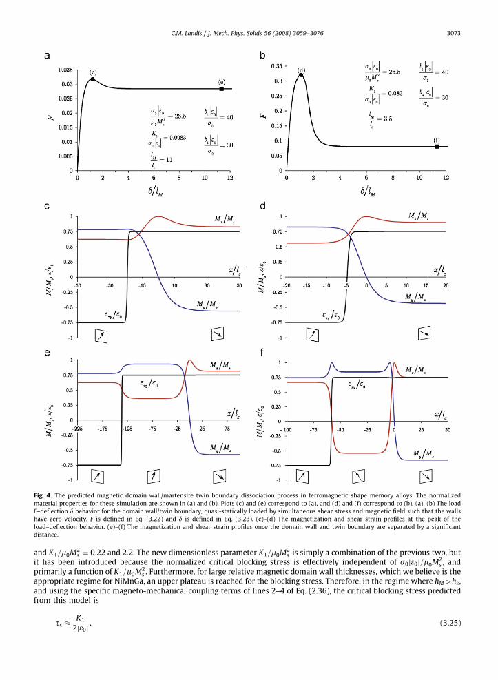
Figs. 1–3 plot the magnetization, stress and strain profiles within a 1801 Bloch wall (magnetization rotates within theplane of the wall), a 1801 Neel wall (magnetization rotates out of the plane of the wall), and a 901 domain wall/twinboundary as predicted for both the perfectly coupled theory and the general theory in a bulk crystal. Thin films have notbeen studied in this work, but a recent review of analytical models that predict how thin film geometries affect thestructure of magnetic domain walls can be found in DeSimone et al. (2006). For the perfectly coupled theory, thecoefficients of the f tensor have been set to zero to obtain more reasonable results. Inclusion of these coefficients makesthe walls predicted by the perfectly coupled theory even thinner, and the stresses within the walls even higher. In general,the additional energy associated with the magneto-mechanical coupling tends to thin the magnetic domain walls and themartensite twin boundaries. In fact, the perfectly coupled theory takes this coupling to the extreme and generates verythin walls.

All strain values are normalized by the magnitude of the spontaneous strain j�0j. Note that the c-axis is shorter than thea-axes in NiMnGa, so the spontaneous strain �0 is less than zero for this material. Two different stress normalizations canbe used, s0 is defined such that s0j�0j is the depth of the energy wells at the spontaneous strain states associated with thefree energy of Eq. (2.36), and sM ¼ K1=j�0j is a characteristic stress that can be used for either the perfectly coupled or moregeneral free energy description. Two length scale normalizations will be used:

l� ¼

ffiffiffiffiffiffiffiffiffiffiffiffia�0j�0j

s0

s(3.16)

and

lM ¼

ffiffiffiffiffiffiffiffiffiffiffiffiffiaM

0 M2s

K1

s. (3.17)

Again, this second length scale can be used with either free energy description. The domain wall and twin boundarythicknesses hM and h� from any given calculation will be defined as:

hM ¼Mþy �M�yðdMy=dxÞjMy¼0

and h� ¼�þxy � �

�xy

ðd�xy=dxÞj�xy¼0, (3.18)

ARTICLE IN PRESS

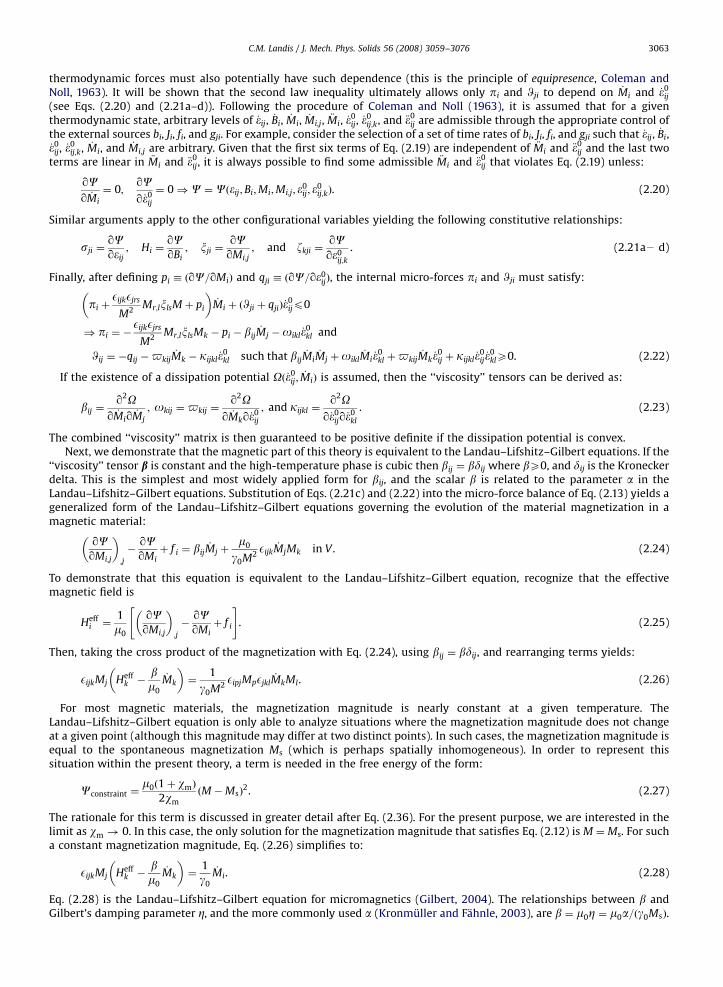
Fig. 1. The magnetization and stress distributions near a 1801 Bloch wall (magnetization rotates in the y–z plane). The arrows in the small inset figure

nominally represent the magnetization on either side of the domain wall located at x ¼ 0. (a)–(b) The magnetization and stress distributions for the

reduced/constrained theory. (c)–(d) The corresponding distributions for the general theory allowing for distinct magnetic domain walls and martensite

twin boundaries.

Table 1Domain wall energies as predicted by the perfectly coupled and general theories assuming that the 1801 Bloch walls in either theory are 20 nm thick

g180Bloch (mJ/m2) g180

Neel (mJ/m2) g90twin (mJ/m2)

Perfectly coupled theory 2220 1750 1040

General theory 8 13 72


where the superscript + and � correspond to the values of the field variable at x ¼ �1. Note that l� and lM are characteristiclength scales associated with fixed material parameters, whereas hM and h� are boundary thicknesses that are computedfrom a solution to the governing field equations.

The domain wall energy is given as:

gwall ¼

Z 1�1

½C�Cð1Þ�dx. (3.19)

For a given set of parameters characteristic of the properties of NiMnGa, Figs. 1–3 indicate that the perfectly coupledtheory gives rise to magnetic domain walls that are approximately one-tenth the thickness of those in the general theory.Additionally, the twin boundary thickness for the perfectly coupled theory must be identical to the magnetic domain wallthickness, whereas the more general theory allows for arbitrary differences in these thicknesses. For the case shown inFig. 3, the magnetic domain wall thickness is approximately three times the twin boundary thickness. Finally, the domain

ARTICLE IN PRESS

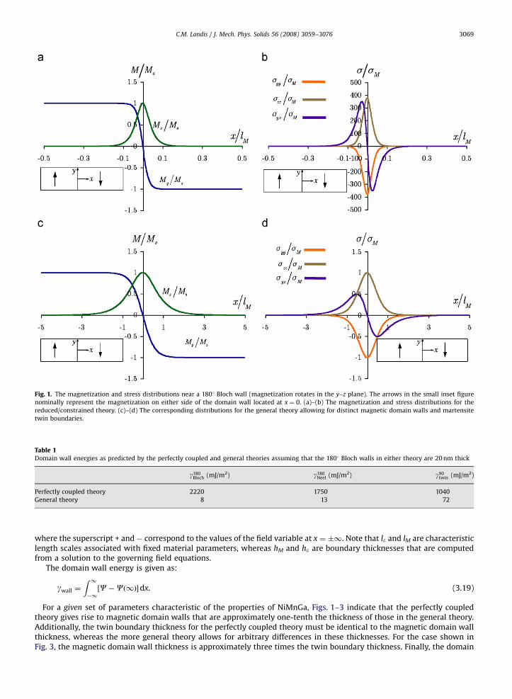
Fig. 2. The magnetization and stress distributions near a 1801 Neel wall (magnetization rotates in the x–y plane). The arrows in the small inset figure

nominally represent the magnetization on either side of the domain wall located at x ¼ 0. (a)–(b) The magnetization and stress distributions for the

reduced/constrained theory. (c)–(d) The corresponding distributions for the general theory allowing for distinct magnetic domain walls and martensite

twin boundaries.


wall energies predicted from the perfectly coupled theory are significantly higher than those from the general theory. Tomake this comparison, it is more informative to apply some representative values for the material coefficients and to scalethe domain wall thicknesses such that they are equal lengths in both theories. Using the parameter values outlined inAppendix and selecting the magnetic domain wall thickness for the 1801 Bloch walls to be 20 nm, the domain wall energiespredicted from each theory are given in Table 1.

Note that these are the energies associated with the simulations plotted in Figs. 1–3. Also note that the f tensor was setto zero in the perfectly coupled theory. If this tensor were included, then the energies for the perfectly coupled theorywould increase by about a factor of 5. We are not aware of any measurements of domain wall energies for NiMnGa;however, magnetic domain walls in many magnetic materials are on the order of 10–20 nm thick and have domain wallenergies in the 10–100 mJ/m2 range. Hence, these computations suggest that the very strong elastic interaction associatedwith the perfectly coupled theory yields an unrealistic description of domain walls in FSMAs. This fact, along with thefeature that the more general theory allows for distinct domain wall and twin boundary length scales, makes the generaltheory a more attractive option for modeling domain structure evolution in ferromagnetic shape memory allows.

Next, the general theory is applied to model the dissociation of a 901 domain wall from its coupled twin boundary. Theappeal of FSMAs is the potential for relatively large actuation strains activated by remote magnetic fields. However, theprimary drawback for these materials is the low blocking stress required to restrict any actuation displacement(Kiefer et al., 2007). In general, every active material has some finite blocking stress for a given actuating field. The methodthat we propose to investigate this phenomenon is through the Eshebly driving traction on a 901 domain wall/twinboundary. Eq. (3.11) indicates that if the driving traction on the coupled wall vanishes then the wall will not move. Thelarge actuating strains that could be achieved by FSMAs can only occur through the motion of domain walls and hence theblocking stress can be determined from Eq. (3.11) by setting the domain wall velocity to zero. Prior to making detailed

ARTICLE IN PRESS

Fig. 3. The magnetization and shear strain and stress distributions near a 901 magnetic domain wall/martensite twin boundary (magnetization rotates in

the x–y plane). The arrows in the small inset figure nominally represent the magnetization on either side of the domain wall located at x ¼ 0. (a)–(b) The

magnetization and shear strain and stress distributions for the reduced/constrained theory. (c)–(d) The corresponding distributions for the general theory

allowing for distinct magnetic domain walls and martensite twin boundaries.


calculations it is instructive to construct an approximation to Eq. (3.11). For an infinite planar domain wall in the y–z planeloaded by a remote magnetic field in the y-direction H and a sxy component of shear stress t the driving force on the wallcan be approximated as:

f � m0

ffiffiffi2p

MsH þ 3�0t. (3.20)

Hereffiffiffi2p

Ms is the jump in the y-component of the magnetization across the domain wall, and 3�0 is the jump in theengineering shear strain across the wall. Note that the constant e0 does carry a sign, and for NiMnGa is less than zero. Thisformula suggests an approximately linear relationship between the blocking stress and the applied magnetic field:

tblock � �m0

ffiffiffi2p

Ms

3�0H. (3.21)

In fact, this result is valid for the perfectly coupled model up to very large levels of H (for H nearly equal to the appliedfield required to cause homogeneous switching of the magnetization). This result is also valid for the general model at lowlevels of applied field. However, within the general theory, due to the independence of the magnetic domain wall from thetwin boundary, there exists some level of applied shear stress such that no level of applied field, no matter how large, cancause actuation. The mechanism for this phenomenon is that the magnetic wall is driven in one direction separately fromthe twin boundary, which moves away in the opposite direction. We refer to this phenomenon as domain wall/twin

boundary dissociation.To elucidate this mechanism, consider only the equilibrium states of a coupled martensite twin boundary and magnetic

domain wall. Furthermore, consider a loading state such that the applied magnetic field tends to move the magnetic wall to

ARTICLE IN PRESS


the right and the applied shear stress tends to move the twin boundary to the left. For relatively low load levels, if the shearstress is less than tblock then no equilibrium state can be found and the magnetic wall and twin boundary move in concertto the right due to the dominating magnetic field. However, if the applied shear stress is greater than tblock, then once againno equilibrium state can be found and the magnetic wall and twin boundary move together to the left due to thedominating shear stress. Equilibrium states of the domain wall can only be found when the applied shear stress is equal totblock. The calculations performed in this work investigate such states. For low levels of applied loading in the appropriateproportions, the magnetic wall tends to move to the right and the twin boundary tends to move to the left. However, due tothe coupling between the walls this relative separation is limited, and an equilibrium configuration with zero wallvelocities can be found. As the applied magneto-mechanical loading is increased, again in the appropriate proportions so asto maintain equilibrium, the relative separation between the magnetic wall and twin boundary increases. Eventually, amaximum is attained in the loading versus relative separation behavior, such that equilibrium states at higher load levelscannot be found. Above this maximum load level, the magnetic wall moves off to the right and the twin boundary movesoff to the left, which is what is referred to as domain wall/twin boundary dissociation. Detailed calculations of this behaviorare presented next.

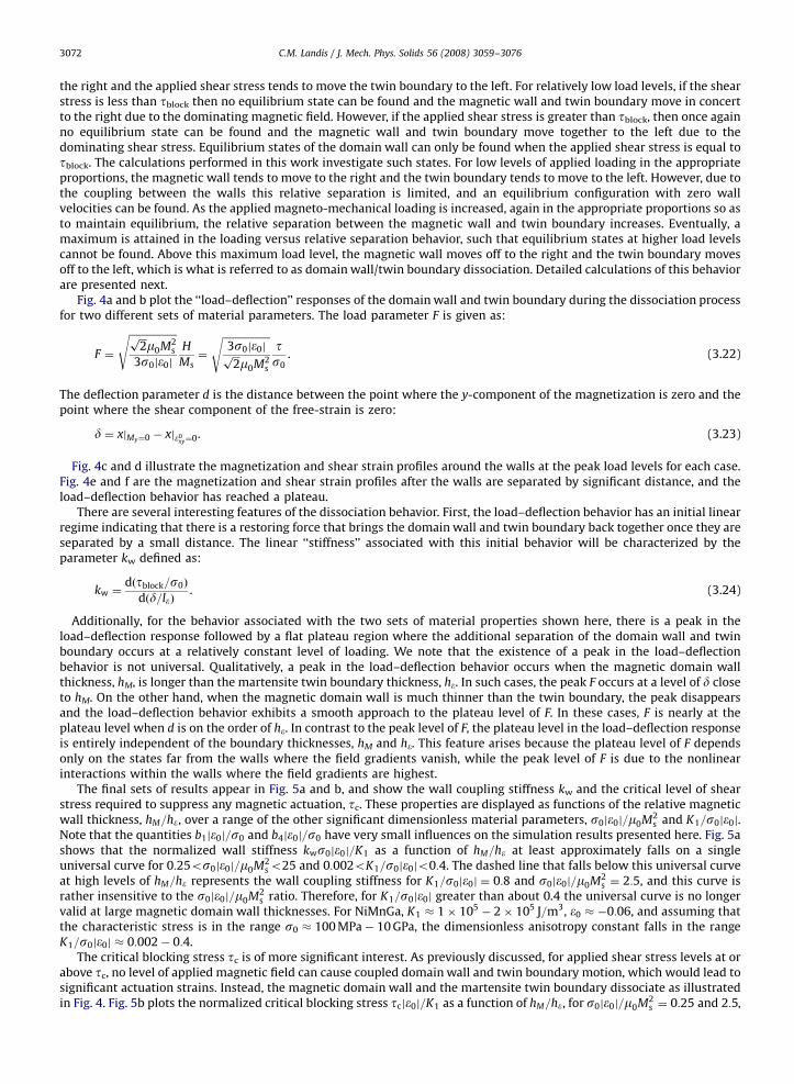
Fig. 4a and b plot the ‘‘load–deflection’’ responses of the domain wall and twin boundary during the dissociation processfor two different sets of material parameters. The load parameter F is given as:

F ¼

ffiffiffiffiffiffiffiffiffiffiffiffiffiffiffiffiffiffiffiffiffiffi2p

m0M2s

3s0j�0j

sH

Ms¼

ffiffiffiffiffiffiffiffiffiffiffiffiffiffiffiffiffiffiffi3s0j�0jffiffiffi2p

m0M2s

sts0

. (3.22)

The deflection parameter d is the distance between the point where the y-component of the magnetization is zero and thepoint where the shear component of the free-strain is zero:

d ¼ xjMy¼0 � xj�0xy¼0. (3.23)

Fig. 4c and d illustrate the magnetization and shear strain profiles around the walls at the peak load levels for each case.Fig. 4e and f are the magnetization and shear strain profiles after the walls are separated by significant distance, and theload–deflection behavior has reached a plateau.

There are several interesting features of the dissociation behavior. First, the load–deflection behavior has an initial linearregime indicating that there is a restoring force that brings the domain wall and twin boundary back together once they areseparated by a small distance. The linear ‘‘stiffness’’ associated with this initial behavior will be characterized by theparameter kw defined as:

kw ¼dðtblock=s0Þ

dðd=l�Þ. (3.24)

Additionally, for the behavior associated with the two sets of material properties shown here, there is a peak in theload–deflection response followed by a flat plateau region where the additional separation of the domain wall and twinboundary occurs at a relatively constant level of loading. We note that the existence of a peak in the load–deflectionbehavior is not universal. Qualitatively, a peak in the load–deflection behavior occurs when the magnetic domain wallthickness, hM, is longer than the martensite twin boundary thickness, he. In such cases, the peak F occurs at a level of d closeto hM. On the other hand, when the magnetic domain wall is much thinner than the twin boundary, the peak disappearsand the load–deflection behavior exhibits a smooth approach to the plateau level of F. In these cases, F is nearly at theplateau level when d is on the order of he. In contrast to the peak level of F, the plateau level in the load–deflection responseis entirely independent of the boundary thicknesses, hM and he. This feature arises because the plateau level of F dependsonly on the states far from the walls where the field gradients vanish, while the peak level of F is due to the nonlinearinteractions within the walls where the field gradients are highest.

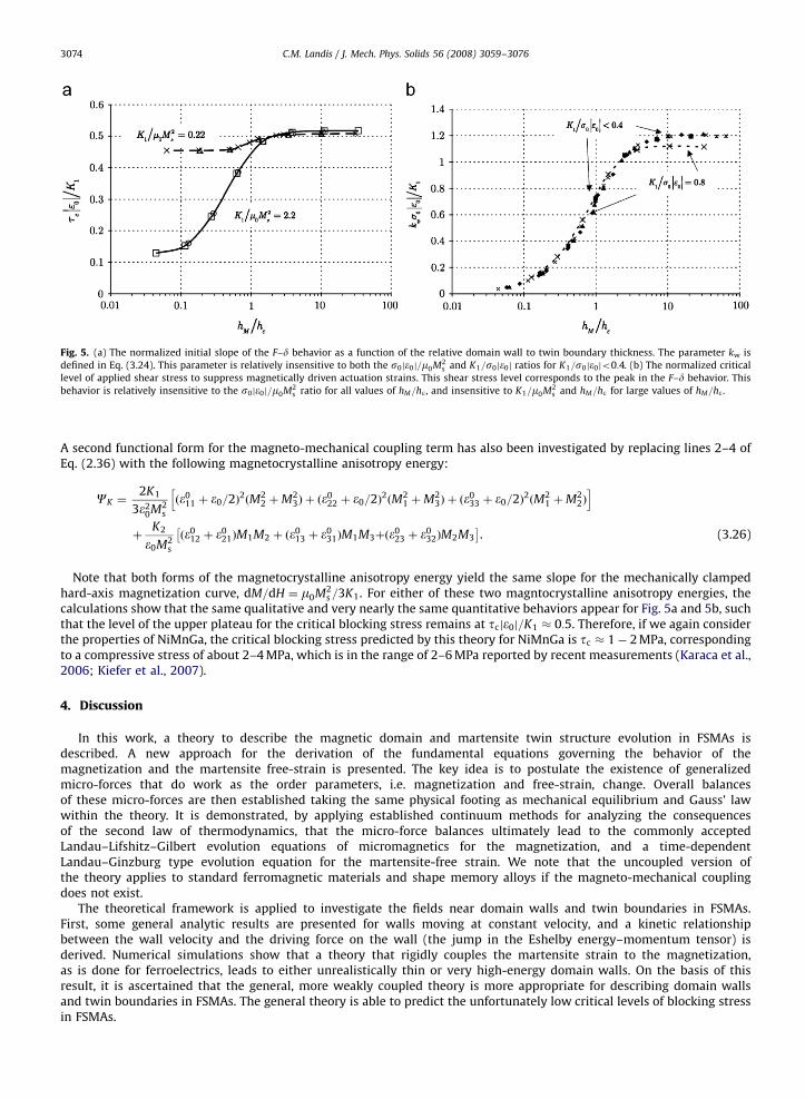
The final sets of results appear in Fig. 5a and b, and show the wall coupling stiffness kw and the critical level of shearstress required to suppress any magnetic actuation, tc. These properties are displayed as functions of the relative magneticwall thickness, hM=h�, over a range of the other significant dimensionless material parameters, s0j�0j=m0M2

s and K1=s0j�0j.Note that the quantities b1j�0j=s0 and b4j�0j=s0 have very small influences on the simulation results presented here. Fig. 5ashows that the normalized wall stiffness kws0j�0j=K1 as a function of hM=h� at least approximately falls on a singleuniversal curve for 0:25os0j�0j=m0M2

so25 and 0:002oK1=s0j�0jo0:4. The dashed line that falls below this universal curveat high levels of hM=h� represents the wall coupling stiffness for K1=s0j�0j ¼ 0:8 and s0j�0j=m0M2

s ¼ 2:5, and this curve israther insensitive to the s0j�0j=m0M2

s ratio. Therefore, for K1=s0j�0j greater than about 0.4 the universal curve is no longervalid at large magnetic domain wall thicknesses. For NiMnGa, K1 � 1� 105

� 2� 105 J=m3, �0 � �0:06, and assuming thatthe characteristic stress is in the range s0 � 100 MPa� 10 GPa, the dimensionless anisotropy constant falls in the rangeK1=s0j�0j � 0:002� 0:4.

The critical blocking stress tc is of more significant interest. As previously discussed, for applied shear stress levels at orabove tc, no level of applied magnetic field can cause coupled domain wall and twin boundary motion, which would lead tosignificant actuation strains. Instead, the magnetic domain wall and the martensite twin boundary dissociate as illustratedin Fig. 4. Fig. 5b plots the normalized critical blocking stress tcj�0j=K1 as a function of hM=h�, for s0j�0j=m0M2

s ¼ 0:25 and 2:5,

ARTICLE IN PRESS

Fig. 4. The predicted magnetic domain wall/martensite twin boundary dissociation process in ferromagnetic shape memory alloys. The normalized

material properties for these simulation are shown in (a) and (b). Plots (c) and (e) correspond to (a), and (d) and (f) correspond to (b). (a)–(b) The load

F–deflection d behavior for the domain wall/twin boundary, quasi-statically loaded by simultaneous shear stress and magnetic field such that the walls

have zero velocity. F is defined in Eq. (3.22) and d is defined in Eq. (3.23). (c)–(d) The magnetization and shear strain profiles at the peak of the

load–deflection behavior. (e)–(f) The magnetization and shear strain profiles once the domain wall and twin boundary are separated by a significant

distance.


and K1=m0M2s ¼ 0:22 and 2:2. The new dimensionless parameter K1=m0M2

s is simply a combination of the previous two, butit has been introduced because the normalized critical blocking stress is effectively independent of s0j�0j=m0M2

s , andprimarily a function of K1=m0M2

s . Furthermore, for large relative magnetic domain wall thicknesses, which we believe is theappropriate regime for NiMnGa, an upper plateau is reached for the blocking stress. Therefore, in the regime where hM4h�,and using the specific magneto-mechanical coupling terms of lines 2–4 of Eq. (2.36), the critical blocking stress predictedfrom this model is

tc �K1

2j�0j. (3.25)

ARTICLE IN PRESS

Fig. 5. (a) The normalized initial slope of the F–d behavior as a function of the relative domain wall to twin boundary thickness. The parameter kw is

defined in Eq. (3.24). This parameter is relatively insensitive to both the s0j�0j=m0M2s and K1=s0j�0j ratios for K1=s0j�0jo0:4. (b) The normalized critical

level of applied shear stress to suppress magnetically driven actuation strains. This shear stress level corresponds to the peak in the F–d behavior. This

behavior is relatively insensitive to the s0j�0j=m0M2s ratio for all values of hM=h� , and insensitive to K1=m0M2

s and hM=h� for large values of hM=h� .


A second functional form for the magneto-mechanical coupling term has also been investigated by replacing lines 2–4 ofEq. (2.36) with the following magnetocrystalline anisotropy energy:

CK ¼2K1

3�20M2

s

ð�011 þ �0=2Þ2ðM2

2 þM23Þ þ ð�

022 þ �0=2Þ2

hðM2

1 þM23Þ þ ð�

033 þ �0=2Þ2ðM2

1 þM22Þ

iþ

K2

�0M2s

ð�012 þ �

021ÞM1M2 þ ð�0

13 þ �031ÞM1M3

�þð�0

23 þ �032ÞM2M3

�. (3.26)

Note that both forms of the magnetocrystalline anisotropy energy yield the same slope for the mechanically clampedhard-axis magnetization curve, dM=dH ¼ m0M2

s =3K1. For either of these two magntocrystalline anisotropy energies, thecalculations show that the same qualitative and very nearly the same quantitative behaviors appear for Fig. 5a and 5b, suchthat the level of the upper plateau for the critical blocking stress remains at tcj�0j=K1 � 0:5. Therefore, if we again considerthe properties of NiMnGa, the critical blocking stress predicted by this theory for NiMnGa is tc � 1� 2 MPa, correspondingto a compressive stress of about 2–4 MPa, which is in the range of 2–6 MPa reported by recent measurements (Karaca et al.,2006; Kiefer et al., 2007).

4. Discussion

In this work, a theory to describe the magnetic domain and martensite twin structure evolution in FSMAs isdescribed. A new approach for the derivation of the fundamental equations governing the behavior of themagnetization and the martensite free-strain is presented. The key idea is to postulate the existence of generalizedmicro-forces that do work as the order parameters, i.e. magnetization and free-strain, change. Overall balancesof these micro-forces are then established taking the same physical footing as mechanical equilibrium and Gauss’ lawwithin the theory. It is demonstrated, by applying established continuum methods for analyzing the consequencesof the second law of thermodynamics, that the micro-force balances ultimately lead to the commonly acceptedLandau–Lifshitz–Gilbert evolution equations of micromagnetics for the magnetization, and a time-dependentLandau–Ginzburg type evolution equation for the martensite-free strain. We note that the uncoupled version ofthe theory applies to standard ferromagnetic materials and shape memory alloys if the magneto-mechanical couplingdoes not exist.

The theoretical framework is applied to investigate the fields near domain walls and twin boundaries in FSMAs.First, some general analytic results are presented for walls moving at constant velocity, and a kinetic relationshipbetween the wall velocity and the driving force on the wall (the jump in the Eshelby energy–momentum tensor) isderived. Numerical simulations show that a theory that rigidly couples the martensite strain to the magnetization,as is done for ferroelectrics, leads to either unrealistically thin or very high-energy domain walls. On the basis of thisresult, it is ascertained that the general, more weakly coupled theory is more appropriate for describing domain wallsand twin boundaries in FSMAs. The general theory is able to predict the unfortunately low critical levels of blocking stressin FSMAs.

ARTICLE IN PRESS


It is postulated that the dissociation of 901 magnetic domain walls and the martensite twin boundaries is themechanism responsible for the low critical blocking stress in FSMAs. This mechanism is studied within numericalsimulations where combined states of shear stress and magnetic field are applied to the material such that the domainwall/twin boundary system remains stationary. At low levels of combined loading, the walls remain connected with theirseparation governed by an elastic type of behavior. As the combined loading is increased, a peak is eventually reached suchthat the magnetic domain wall and the martensite twin boundary move in opposite directions. The implication from thisbehavior is that if the applied stress is higher than this peak, then no level of applied magnetic field is able to drive coupleddomain wall/twin boundary motion, and hence no significant actuating strain can be produced. The theory places thecritical compressive blocking stress for NiMnGa in the range of 2–4 MPa, which is in agreement with experimentalobservations.

Acknowledgment

The author would like to acknowledge support from the National Science Foundation under project number CMMI-0719071.

Appendix

The specific form for the Helmholtz-free energy applied in this work is given in Eq. (2.36) and is repeated below. In acoordinate system with the Cartesian axes aligned with the /10 0S directions, this form of the free energy that can be usedto mimic the properties of single crystals with a tetragonal martensite phase and an easy magnetization axis aligned withthe c-axis of the unit cell:

c ¼1

2aM

0 Mi;jMi;j þ1

2a�0�

0ij;k�

0ij;k

þK1

�0M2s

�011 þ

�0

2

� �ðM2

2 þM23Þ þ �0

22 þ�0

2

� �hðM2

1 þM23Þ þ ð�

033 þ �0=2ÞðM2

1 þM22Þ

i�

2

3

K1

�20

½�011�

022 þ �

011�

033 þ �

022�

033 þ �0ð�0

11 þ �022 þ �

033�

þK2

�0M2s

½ð�012 þ �

021ÞM1M2 þ ð�0

13 þ �031ÞM1M3 þ ð�0

23 þ �032ÞM2M3�

þb1

2ð�0

kkÞ2þ

b2

3½ðe0

11Þ3þ ðe0

22Þ3þ ðe0

33Þ3� þ

b3

4½ðe0

11Þ4þ ðe0

22Þ4þ ðe0

33Þ4�

þb4

2½ð�0

12Þ2þ ð�0

21Þ2þ ð�0

13Þ2þ ð�0

31Þ2þ ð�0

23Þ2þ ð�0

32Þ2� þ

1


ijÞð�kl � �0klÞ

þ1

2m0

BiBi �MiBi þm0ð1þ wmÞ

2wm

ðM �MsÞ2þ m0MsM, (A.1)

e0ij ¼ �

0ij �

13�

0kkdij and M ¼

ffiffiffiffiffiffiffiffiffiffiffiffiMiMi

p. (A.2)

For our calculations we have chosen values for these parameters that mimic NiMnGa. It is useful to express theseparameters in dimensionless form. To do this, we introduce a characteristic stress, s0, such that the height of the energybarrier given by the b-terms is s0�0. This then implies that

b2 ¼ �16s0�0

j�30j

and b3 ¼32

3

s0

j�30j

. (A.3)

For a martensite variant with its c-axis oriented in the x1-direction, the curvature components of the energy wells definedby Eq. (2.41) are then:

f 1111 ¼ b1 þ16

3

s0

j�0j; f 2222 ¼ f 3333 ¼ b1 þ

40

3

s0

j�0j,

f 1122 ¼ f 1133 ¼ b1 �8

3

s0

j�0j; f 2233 ¼ b1 �

32

3

s0

j�0j. (A.4)

The characteristic values for NiMnGa are: Ms ¼ 6�105 A/m, �0 ¼ �0:06, s0 ¼ 200 MPa, b1 ¼ 40s0=j�0j, b4 ¼ 30s0=j�0j,K1 ¼ K2 ¼ 1� 105

� 2� 105 J/m3, m0 ¼ 4p� 10�7 N/A2, wm ¼ 10�5, and the principal values of cijkl are 105s0=j�0j. Theparameter ranges that have been investigated in this paper surround these values. These choices for the parameters lead toelastic properties very similar to those measured by Dai et al. (2004), and yield a slope for the hard-axis, mechanicallyclamped M–H curve of dM=dH ¼ m0M2

s =3K1. The choices for a0M and a0

� simply set the length scales within the problem asdefined by Eqs. (3.16) and (3.17).

ARTICLE IN PRESS


References

Brown, W.F., 1963. Micromagnetics. Wiley, New York, USA.Chen, L.Q., 2002. Phase-field models for microstructure evolution. Ann. Rev. Mater. Res. 32, 113–140.Coleman, R.D., Noll, W., 1963. The thermodynamics of elastic materials with heat conduction and viscosity. Arch. Rational Mech. Anal. 13, 167–178.Dai, L., Cullen, J., Wuttig, M., 2004. Intermartensitic transformation in a NiMnGa alloy. J. Appl. Phys. 95, 6957–6959.DeSimone, A., James, R.D., 1997. A theory of magnetostriction oriented to-wards applications. J. Appl. Phys. 81, 5706–5708.DeSimone, A., James, R.D., 2002. A constrained theory of magnetoelasticity. J. Mech. Phys. Solids 50, 283–320.DeSimone, A., Kohn, R.V., Muller, S., Otto, F., 2006. Recent analytical developments in micromagnetics. In: Berotti, G., Mayergoyz, I. (Eds.), The Science of

Hysteresis II: Physical Modeling, Micromagnetics, and Magnetization Dynamics. Elsevier, pp. 269–381.Eshelby, J.D., 1970. Energy relations and the energy–momentum tensor in continuum mechanics. Inelastic Behav. Solids, 77–115.Fried, E., Gurtin, M.E., 1993. Continuum theory of thermally induced phase transitions based on an order parameter. Physica D 68, 326–343.Fried, E., Gurtin, M.E., 1994. Dynamic solid–solid transitions with phase characterized by an order parameter. Physica D 72, 287–308.Gilbert, T.L., 1956. Formulation, foundations, and applications of the phenomenological theory of ferromagnetism. PhD Thesis. Illinois Institute of

Technology.Gilbert, T.L., 2004. A phenomenological theory of damping in ferromagnetic materials. IEEE Trans. Magn. 40, 3443–3449.Givoli, D., Keller, J.B., 1989. A finite-element method for large domains. Comput. Methods Appl. Mech. Eng. 76, 41–66.Gurtin, M.E., 1996. Generalized Ginzburg–Landau and Cahn–Hilliard equations based on a microforce balance. Physica D 92, 178–192.Gurtin, M.E., Weissmuller, J., Larche, F., 1998. A general theory for curved deformable interfaces in solids at equilibrium. Philos. Mag. A 78, 1093–1109.James, R.D., Wuttig, M., 1998. Magnetostriction of martenstite. Philos. Mag. A 77, 1273–1299.Jin, Y.M., Artemev, A., Khachaturyan, A.G., 2001. Three-dimensional phase field model of low-symmetry martensitic transformation in polycrystal:

simulation of z’2 martensite in AuCd alloys. Acta Mater. 49, 2309–2320.Karaca, H.E., Karaman, I., Basaran, B., Chumlyakov, Y.I., Maier, H.J., 2006. Magnetic field and stress induced martensite reorientation in NiMnGa

ferromagnetic shape memory alloy single crystals. Acta Mater. 54, 233–245.Kiefer, B., Lagoudas, D.C., 2005. Magnetic field-induced martensitic reorientation in magnetic shape memory alloys. Philos. Mag. 85, 4289–4329.Kiefer, B., Karaca, H.E., Lagoudas, D.C., Karaman, I., 2007. Characterization and modeling of the magnetic field-induced strain and work output in magnetic

shape memory alloys. J. Magn. Magn. Mater. 312, 164–175.Kronmuller, H., Fahnle, M., 2003. Micromagnetism and the Microstructure of Ferromagnetic Solids. Cambridge University Press.Landau, L.D., Lifsitz, E.M., 1935. On the theory of the dispersion of magnetic permeability in ferromagnetic bodies. Phys. Z. Sowjet 8, 153–169.Ma, Y.F., Li, J.Y., 2007a. A constrained theory on actuation strain in ferro-magnetic shape memory alloys induced by domain switching. Acta Mater. 55,

3261–3269.Ma, Y.F., Li, J.Y., 2007b. Magnetization rotation and rearrangement of martensite variants in ferromagnetic shape memory alloys. Appl. Phys. Lett. 90,

172504.Murray, S.J., Marioni, M., Tello, P.G., Allen, S.M., O’Handley, R.C., 2001. Giant magnetic-filed-induced strain in Ni–Mn–Ga crystals: experimental results and

modeling. J. Magn. Magn. Mater. 226–230, 945–947.Nye, J.F., 1957. Physical Properties of Crystals. Oxford University Press, Great Britain.O’Handley, R.C., Murray, S.J., Marioni, M., Nembach, H., Allen, S.M., 2000. Phenomenology of giant magnetic-field-induced strain in ferromagnetic shape-

memory alloys. J. Appl. Phys. 87, 4712–4717.Sozinov, A., Likhachev, A.A., Lanska, N., Ullakko, K., 2002. Giant magnetic-field-induced strain in NiMnGa seven-layered martensitic phase. Appl. Phys. Lett.

80, 1746–1748.Su, Y., Landis, C.M., 2007. Continuum thermodynamics of ferroelectric domain evolution: theory, finite element implementation, and application to

domain wall pinning. J. Mech. Phys. Solids 55, 280–305.Thiele, A.A., 1974. Applications of the gyrocoupling vector and dissipation dyadic in the dynamics of magnetic domains. J. Appl. Phys. 45, 377–393.Tickle, R., 2000. Ferromagnetic shape memory materials. PhD Thesis. University of Minnesota.Tickle, R., James, R.D., 1999. Magnetic and magnetomechanical properties of Ni2MnGa. J. Magn. Magn. Mater. 195, 627–638.Wang, Y.U., Jin, Y.M., Khachaturyan, A.G., 2004. The effects of free surfaces on martensite microstructures: 3D phase field microelasticity simulation study.

Acta Mater. 52, 1039–1050.Zhang, J.X., Chen, L.Q., 2005a. Phase-field model for ferromagnetic shape-memory alloys. Philos. Mag. Lett. 85, 533–541.Zhang, J.X., Chen, L.Q., 2005b. Phase-field microelasticity theory and micromagnetic simulations of domain structures in giant magnetostrictive materials.

Acta Mater. 53, 2845–2855.

a continuum thermodynamics formulation for micro-magneto ...landis/landis/research... · a...

Documents