J. Math. Anal. Appl. 409 (2014) 485–493

Contents lists available at ScienceDirect

Journal of Mathematical Analysis andApplications

journal homepage: www.elsevier.com/locate/jmaa

A continuous method for nonlocal functional differentialequations with delayed or advanced argumentsX.Y. Li a, B.Y. Wu b,∗

a Department of Mathematics, Changshu Institute of Technology, Suzhou, Jiangsu 215500, Chinab Department of Mathematics, Harbin Institute of Technology, Harbin, Heilongjiang 150001, China

a r t i c l e i n f o

Article history:Received 29 December 2012Available online 23 July 2013Submitted by M. Laczkovich

Keywords:Reproducing kernel methodNonlocal problemsFunctional differential equationsError estimation

a b s t r a c t

In the previous works, the authors presented the reproducing kernel method (RKM) forsolving various differential equations. However, to the best of our knowledge, there existno results for functional differential equations. The aim of this paper is to extend theapplication of reproducing kernel theory to nonlocal functional differential equations withdelayed or advanced arguments, and give the error estimation for the present method.Some numerical examples are provided to show the validity of the present method.

© 2013 Elsevier Inc. All rights reserved.

1. Introduction

Reproducing kernel theory has important application in numerical analysis, differential equations, probability andstatistics, learning theory and so on. Recently, reproducing kernelmethods for solving a variety of differential equationswerepresented by Cui and Geng [4–9], Lin and Zhou [12,13], Yao, Chen and Jiang [3,26], Wang, Li and Wu [11,22], Mohammadiand Mokhtari [15], Akram and Ur Rehman [1], Arqub, Al-Smadi, Momani [2], Özen and Oruçoğlu [17], Wang, Han andYamamoto [23].

In this paper, we consider the following functional differential equations with linear nonlocal conditions:u′(x)+ a(x)u(x)+ b(x)u(τ (x)) = f (x), x ∈ I = [0, 1],B(u(c), u) = 0, (1.1)

where c ∈ I, a(x), b(x) ∈ C[0, 1], τ (x) ∈ C1[0, 1], and f is given such that (1.1) satisfies the existence and uniqueness of

the solutions.Notice that function B(u(c), u) = 0 includes several types of boundary conditions: initial conditions, final conditions,

periodic conditions, or more general functional conditions, as

B(u(c), u) = λu(c)−

1

0u(s)ds, λ ∈ R.

Functional differential equations arise in a variety of applications, such as number theory, electrodynamics, astrophysics,nonlinear dynamical systems, probability theory on algebraic structure, quantummechanics and cell growth. Therefore, theproblems have attracted a great deal of attention. Liu and Li [14] studied the analytical and numerical solutions of themulti-pantograph equations. Sezer [20,21] gave the series solutions of multi-pantograph equations with variable coefficients.

∗ Corresponding author.E-mail addresses: lixiuying1112@126.com (X.Y. Li), mathwby@sina.com (B.Y. Wu).

0022-247X/$ – see front matter© 2013 Elsevier Inc. All rights reserved.http://dx.doi.org/10.1016/j.jmaa.2013.07.039

486 X.Y. Li, B.Y. Wu / J. Math. Anal. Appl. 409 (2014) 485–493

Wang, Qin and Li [25] proposed one-leg h-methods for nonlinear neutral differential equations with proportional delay.In [10,16,19], the authors discussed the series solutions of some functional differential equations. Wang, Shen and Luo [24]obtained the existence of solutions of second-order multi-point functional differential equations by using the method ofupper and lower solutions. Rodríguez-López [18] studied the existence of a solution to a nonlocal boundary value problemfor a class of second-order functional differential equations with piecewise constant arguments.

However, numerical solutions of nonlocal functional differential equations are seldom discussed. The aim of this paperis to fill this gap.

The rest of the paper is organized as follows. In the next section, the reproducing kernel method for solving (1.1) isintroduced. The error estimation is presented in Section 3. Numerical examples are provided in Section 4. Section 5 endsthis paper with a brief conclusion.

2. Reproducing kernel method for (1.1)

In this section, we extend the application of reproducing kernel theory to nonlocal functional differential equation (1.1).To solve (1.1), first, we construct reproducing kernel spaces Wm

[0, 1], (m ≥ 2) in which every function satisfies theboundary condition of (1.1).

Definition 2.1. Wm0 [0, 1] = {u(x) | u(m−1)(x) is an absolutely continuous real value function, u(m)(x) ∈ L2[0, 1]}. The inner

product and norm inWm0 [0, 1] are given respectively by

(u, v)m =

m−1i=0

u(i)(0)v(i)(0)+

1

0u(m)(x)v(m)(x)dx

and

∥u∥m =

(u, u)m, u, v ∈ Wm

0 [0, 1].

By [6,8],Wm0 [0, 1] is a reproducing kernel space and its reproducing kernel k0(x, y) can be obtained.

Next, we construct reproducing kernel spaceWm[0, 1] in which every function satisfies B(u(c), u) = 0.

Definition 2.2. Wm[0, 1] = {u(x) | u(x) ∈ Wm

0 [0, 1], B(u(c), u) = 0}.

Clearly,Wm[0, X] is a closed subspace ofWm

0 [0, X] and therefore it is also a reproducing kernel space.Put Pu(x) = B(u(c), u).

Theorem 2.1. If PxPyk(x, y) = 0, then the reproducing kernel K(x, y) of Wm[0, 1] is given by

K(x, y) = k0(x, y)−Pxk0(x, y)Pyk0(x, y)

PxPyk0(x, y),(2.1)

where the subscript x by the operator P indicates that the operator P applies to the function of x.

Proof. It is easy to see that PK(x, y) = 0, and therefore K(x, y) ∈ Wm[0, 1].

For all u(y) ∈ Wm[0, 1], obviously, Pyu(y) = 0, it follows that

(u(y), K(x, y))m = (u(y), k0(x, y))m = u(x).

That is, K(x, y) is of ‘‘reproducing property’’. Thus, K(x, y) is the reproducing kernel of Wm[0, 1] and the proof is

complete. �

In [6], Cui and Lin defined reproducing kernel spaceW 1[0, 1] and gave its reproducing kernel

k(x, y) =

1 + y, y ≤ x,1 + x, y > x.

Put

Lu(x) = u′(x)+ a(x)u(x)+ b(x)u(τ (x)).

Theorem 2.2. L : Wm[0, 1] → W 1

[0, 1] is a bounded linear operator.

Proof. It is easy to see that

|u(x)| = |(u(·), K(x, ·))m|

≤ ∥u(·)∥m ∥K(x, ·)∥m. (2.2)

X.Y. Li, B.Y. Wu / J. Math. Anal. Appl. 409 (2014) 485–493 487

Similarly,

|u′(x)| =

u(·), ∂K(x, ·)∂x

m

≤ ∥u(·)∥m

∂K(x, ·)∂x

m

(2.3)

and

|u′′(x)| ≤ ∥u(·)∥m

∂2 K(x, ·)∂x2

m. (2.4)

By (2.2) and (2.3), there exists a positive constantM1 such that

∥b(x)u(x)∥1 ≤ ∥b(x)∥1 ∥u(x)∥1

≤ M0

u2(0)+

1

0(u′(x))2dx

1/2≤ M0

∥u∥2

m ∥K(0, ·)∥2m + ∥u(·)∥2

m

1

0

∂K(x, ·)∂x

2mdx

1/2

≤ M1∥u∥m. (2.5)

Similarly, we have

∥a(x)u(τ (x))∥1 ≤ ∥a(x)∥1 ∥u(τ (x))∥1

≤ M2

u2(τ (0))+

1

0(u′(τ (x))τ ′(x))2dx

1/2≤ M3

∥u∥2

m ∥K(0, ·)∥2m + ∥u(·)∥2

m

1

0

∂K(x, ·)∂x

2mdx

1/2

≤ M4∥u∥m (2.6)

where M2,M3 andM4 are positive constants.Combining (2.3) and (2.4), there exists a positive constantM5 such that

∥u′(x)∥1 =

(u′(0))2 +

1

0(u′′(x))2dx

1/2≤ M5∥u∥m. (2.7)

From (2.5)–(2.7), it follows that

∥Lu∥1 ≤ (M1 + M4 + M5)∥u∥m

≤ M∥u∥m,

whereM is a positive constant.Therefore, L : Wm

[0, 1] → W 1[0, 1] is a bounded linear operator and the proof is complete. �

Putϕi(x) = k(xi, x) andψi(x) = L∗ϕi(x)where k(xi, x) is the reproducing kernel ofW 1[0, 1], L∗ is the adjoint operator of L.

The orthonormal system {ψ i(x)}∞

i=1 ofWm[0, 1] can be derived fromGram–Schmidt orthogonalization process of {ψi(x)}∞i=1,

ψ i(x) =

ik=1

βikψk(x), (βii > 0, i = 1, 2, . . .). (2.8)

According to [6,8], we have the following theorem:

Theorem 2.3. If {xi}∞i=1 is dense in [0, 1], then {ψi(x)}∞i=1 is the complete system of Wm[0, 1] and ψi(x) = LsK(x, s)|s=xi .

Theorem 2.4. If {xi}∞i=1 is dense in [0, 1] and the solution of (1.1) is unique, then the solution of (1.1) is

u(x) =

∞j=1

Ajψ j(x), (2.9)

where Aj =j

l=1 βjlf (xl).

488 X.Y. Li, B.Y. Wu / J. Math. Anal. Appl. 409 (2014) 485–493

Now, the approximate solution u(x) can be obtained by taking finitely many terms in the series representation of u(x)and

uN(x) =

Nj=1

Ajψ j(x). (2.10)

Remark. Since Wm[0, 1] is a Hilbert space, it is clear that

∞

i=1(i

k=1 βikf (xk))2 < ∞. Therefore, the sequence uN isconvergent in the sense of norm ∥ · ∥m.

Lemma 2.1. If u(x) ∈ Wm[0, 1], then there exists a constant C such that |u(x)| ≤ C∥u(x)∥m, |u(k)(x)| ≤ C∥u(x)∥m, 1 ≤ k ≤

m − 1.

Proof. Since

|u(x)| = |(u(y), k(x, y))m| ≤ ∥u(y)∥m ∥k(x, y)∥m,

there exists a constant c0 such that

|u(x)| ≤ c0∥u∥m.

Note that

|u(i)(x)| =

u(y), ∂ ik(x, y)∂xi

m

≤ ∥u∥m

∂ ik(x, y)∂xi

m

≤ ci∥u∥m, (i = 0, 1, 2, . . . ,m − 1),

where ci are constants.Putting C = max0≤i≤m−1{ci} and the proof of the lemma is complete. �

From the above lemma and convergence of un(x) in the sense of norm, it is easy to obtain the following theorem.

Theorem 2.5. The approximate solution un(x) and its derivatives u(k)n (x), 1 ≤ k ≤ m − 1 are all uniformly convergent.

3. Error estimations

To give the error estimation for the solution of (1.1) it is assumed that b(x) < 0, a(x)+ b(x) ≥ α > 0.

Lemma 3.1. Let u(x) ∈ C1[0, 1]. If u(0) ≥ 0, Lu ≥ 0, ∀x ∈ I , then u ≥ 0, ∀x ∈ I .

Proof. It can be easily proven by contradiction. Suppose x∗∈ (0, 1) be such that

u(x∗) = minx∈(0,1)

u(x), u(x∗) < 0.

Then it is clear that u′(x∗) = 0, therefore we have

Lu(x)|x=x∗ = a(x∗)u(x∗)+ b(x∗)u(τ (x∗)).

From b(x) < 0 and a(x)+ b(x) ≥ α > 0, it follows that

Lu(x)|x=x∗ ≤ a(x∗)u(x∗)+ b(x∗)u(x∗) = [a(x∗)+ b(x∗)]u(x∗) < 0

which is a contradiction. �

Lemma 3.2. The solution of (1.1) satisfies

|u(x)| ≤ D max|u(0)|, max

x∈(0,1)|Lu|

,

where D is a positive constant and D ≥1α.

Proof. Define two functions

φ±(x) = D max|u(0)|, max

x∈(0,1)|Lu|

± u(x),

where D is a positive constant and D ≥1α.

X.Y. Li, B.Y. Wu / J. Math. Anal. Appl. 409 (2014) 485–493 489

It is clear that φ±(0) ≥ 0, and

Lφ±(x) = D [a(x)+ b(x)]max|u(0)|, max

x∈(0,1)|Lu|

± Lu(x)

≥ max|u(0)|, max

x∈(0,1)|Lu|

± Lu(x)

≥ 0.

By Lemma 3.1, we get

|u(x)| ≤ D max|u(0)|, max

x∈(0,1)|Lu|

. �

Theorem 3.1. Let uN(x) be the approximate solution of (1.1) in space W 3[0, 1] and u(x) be the exact solution of (1.1). If

0 = x1 < x2 < · · · < xN = 1, a(x), b(x), τ (x), f (x) ∈ C2[0, 1], and if |u(0)| ≤ |Lu(0)|, then

∥u(x)− uN(x)∥∞ ≤ d1 h2,

where ∥u(x)∥∞ = maxx∈[0,1] |u(x)|, d1 is a positive constant, h = max1≤i≤N−1 |xi+1 − xi|.

Proof. Note here that

LuN(x) =

Ni=1

AiLψ i(x)

and

(LuN)(xn) =

Ni=1

Ai(Lψ i, ϕn) =

Ni=1

Ai(ψ i, L∗ϕn) =

Ni=1

Ai(ψ i, ψn).

Therefore,

nj=1

βnj(LuN)(xj) =

Ni=1

Ai

ψ i,

nj=1

βnjψj

=

Ni=1

Ai(ψ i, ψn) = An. (3.1)

If n = 1, then (LuN)(x1) = f (x1).If n = 2, then β21(LuN)(x1)+ β22(LuN)(x2) = β21f (x1)+ β22f (x2).It is clear that (LuN)(x2) = f (x2).Moreover, it is easy to see by induction that

(LuN)(xj) = f (xj), j = 1, 2, . . . ,N. (3.2)

Put RN(x) = f (x)− LuN(x). Obviously, RN(x) ∈ C2[0, 1] and RN(xj) = 0, j = 1, 2, . . . ,N . Suppose that l(x) is a polynomial

of degree = 1 that interpolates the function RN(x) at xi, xi+1. It is clear that l(x) = 0. Also, for ∀x ∈ [xi, xi+1],

RN(x) = RN(x)− l(x) =R′′

N(ξi)

2!(x − xi)(x − xi+1), ξi ∈ [xi, xi+1]. (3.3)

Hence, for ∀x ∈ [xi, xi+1],

|RN(x)| ≤|R′′

N(ξi)|

8h2i = cih2

i , ci =|R′′

N(ξi)|

8, hi = |xi+1 − xi|.

Putting cc = max1≤i≤N−1 ci and h = max1≤i≤N−1 hi, we have

∥RN(x)∥∞ = maxx∈[0,1]

|RN(x)| ≤ cc h2.

Obviously, u(x)− uN(x) is the solution of Lv(x) = RN(x).According to Lemma 3.2, there exists a positive constant d1 such that

∥u(x)− uN(x)∥∞ ≤ d1 h2. �

490 X.Y. Li, B.Y. Wu / J. Math. Anal. Appl. 409 (2014) 485–493

Theorem 3.2. Let uN(x) be the approximate solution of (1.1) in space W 4[0, 1] and u(x) be the exact solution of (1.1). If

0 = x1 < x2 < · · · < xN = 1, a(x), b(x), τ (x), f (x) ∈ C4[0, 1], and if |u(0)| ≤ |Lu(0)|, then

∥u(x)− uN(x)∥∞ ≤ d2 h4,

where d2 is a positive constant, h = max1≤i≤N−1 |xi+1 − xi|.

Proof. From the proof of Theorem 3.1, we have

LuN(xj) = f (xj), j = 1, 2, . . . ,N.

Put

RN(x) = f (x)− LuN(x).

Obviously,

RN(x) ∈ C4[0, 1], RN(xj) = 0, j = 1, 2, . . . ,N.

On interval [xi, xi+1], the application of Roll’s theorem to RN(x) yields

R′

N(yi) = 0, yi ∈ (xi, xi+1), i = 1, 2, . . . ,N − 1.

On interval [yi, yi+1], the application of Roll’s theorem to R′

N(x) yields

R′′

N(zi) = 0, zi ∈ (yi, yi+1), i = 1, 2, . . . ,N − 2.

Putting

h = max1≤i≤N−1

{|xi+1 − xi|}, hy = max1≤i≤N−2

{|yi+1 − yi|}, hz = max1≤i≤N−3

{|zi+1 − zi|},

clearly,

hy ≤ 2h, hz ≤ 4h.

Suppose that l1(x) is a polynomial of degree = 1 that interpolates the function R′′

N(x) at z1, z2. It is clear that l1(x) = 0. Also,for ∀x ∈ [x1, z2], there exist η1 ∈ [x1, z2] and a positive constant b1 such that

R′′

N(x) = R′′

N(x)− l1(x) =R(4)N (η1)

2!(x − z1)(x − z2) ≤ b1 h2.

In a similar way, there exist positive constants ci, b2 such that

R′′

N(x) ≤ ci h2, x ∈ [zi, zi+1], i = 2, 3, . . . ,N − 3,

and

R′′

N(x) ≤ b2 h2, x ∈ [zN−2, xN ].

Hence, there exists a positive constant d2 such that

∥R′′

N(x)∥∞ ≤ d2 h2.

On interval [xi, xi+1] i = 1, 2, . . . ,N − 1, noting that

R′

N(x) =

x

yiR′′

N(s)ds,

there exist constants ai

|R′

N(x)| ≤ ∥R′′

N(x)∥∞|x − yi| ≤ ai h3.

It turns out that

∥R′

N(x)∥∞ ≤ a0 h3, x ∈ [x1, xN ] = [0, 1] (3.4)

where a0 is a positive constant.In a similar way, there exists a positive constant a1 such that

∥RN(x)∥∞ ≤ a1 h4, x ∈ [0, 1].

Obviously, u(x)− uN(x) is the solution of Lv(x) = RN(x).According to Lemma 3.2, it is easy to see that

∥u(x)− uN(x)∥∞ ≤ d2 h4,

where d2 is a positive constant. �

X.Y. Li, B.Y. Wu / J. Math. Anal. Appl. 409 (2014) 485–493 491

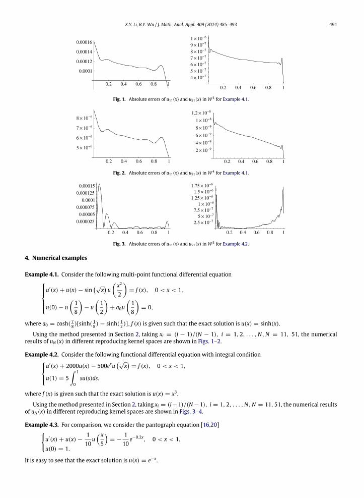
Fig. 1. Absolute errors of u11(x) and u51(x) in W 3 for Example 4.1.

Fig. 2. Absolute errors of u11(x) and u51(x) in W 4 for Example 4.1.

Fig. 3. Absolute errors of u11(x) and u51(x) in W 3 for Example 4.2.

4. Numerical examples

Example 4.1. Consider the following multi-point functional differential equationu′(x)+ u(x)− sin

√xux2

2

= f (x), 0 < x < 1,

u(0)− u18

− u

12

+ a0u

18

= 0,

where a0 = cosh( 78 )[sinh(18 )− sinh( 12 )], f (x) is given such that the exact solution is u(x) = sinh(x).

Using the method presented in Section 2, taking xi = (i − 1)/(N − 1), i = 1, 2, . . . ,N,N = 11, 51, the numericalresults of uN(x) in different reproducing kernel spaces are shown in Figs. 1–2.

Example 4.2. Consider the following functional differential equation with integral conditionu′(x)+ 2000u(x)− 500exu√

x

= f (x), 0 < x < 1,

u(1) = 5 1

0su(s)ds,

where f (x) is given such that the exact solution is u(x) = x3.

Using themethod presented in Section 2, taking xi = (i−1)/(N−1), i = 1, 2, . . . ,N,N = 11, 51, the numerical resultsof uN(x) in different reproducing kernel spaces are shown in Figs. 3–4.

Example 4.3. For comparison, we consider the pantograph equation [16,20]u′(x)+ u(x)−

110

u x5

= −

110

e−0.2x, 0 < x < 1,u(0) = 1.

It is easy to see that the exact solution is u(x) = e−x.

492 X.Y. Li, B.Y. Wu / J. Math. Anal. Appl. 409 (2014) 485–493

Fig. 4. Absolute errors of u11(x) and u51(x) inW 4 for Example 4.2.

Table 1Comparison of absolute error for Example 4.3.

x Muroya [16] Taylor method [20] Present method (N = 11) Present method (N = 151)

2−1 2.19 × 10−5 1.24 × 10−10 1.59 × 10−6 3.33 × 10−11

2−2 1.08 × 10−5 9.74 × 10−11 1.87 × 10−6 4.13 × 10−11

2−3 3.81 × 10−5 7.00 × 10−11 2.71 × 10−6 4.62 × 10−11

2−4 1.26 × 10−5 9.14 × 10−11 2.41 × 10−6 4.89 × 10−11

2−5 4.09 × 10−5 5.28 × 10−11 1.00 × 10−6 5.05 × 10−11

2−6 1.20 × 10−5 1.95 × 10−11 3.51 × 10−7 4.74 × 10−11

In Table 1, the absolute errors of the present method for N = 11, 81 are compared with Muroya method [16] and Taylormethod of [20].

5. Conclusion

In this paper, based on reproducing kernel theory, a continuous method is proposed for solving nonlocal first orderfunctional differential equations with delayed or advanced arguments. Also, the error estimation of the present methodis developed. The results of numerical examples show that the present method can provide accurate approximate solutions.In addition, the present method is also effective for linear functional differential equations with large coefficients.

Acknowledgments

The author would like to express thanks to the unknown referees for their careful reading and helpful comments. Thiswork is supported by the National Natural Science Foundation of China (No. 11126222, 11271100).

References

[1] G. Akram, H. Ur Rehman, Numerical solution of eighth order boundary value problems in reproducing Kernel space, Numer. Algorithms 62 (2013)527–540.

[2] O.A. Arqub,M. Al-Smadi, S.Momani, Application of reproducing kernelmethod for solving nonlinear Fredholm–Volterra integro-differential equations,Abstr. Appl. Anal. 2012 (2012) 1–16.

[3] Z. Chen, W. Jiang, The exact solution of a class of Volterra integral equation with weakly singular kernel, Appl. Math. Comput. 217 (2011) 7515–7519.[4] M.G. Cui, F.Z. Geng, Solving singular two-point boundary value problem in reproducing kernel space, J. Comput. Appl. Math. 205 (2007) 6–15.[5] M.G. Cui, F.Z. Geng, A computational method for solving third-order singularly perturbed boundary-value problems, Appl. Math. Comput. 198 (2008)

896–903.[6] M.G. Cui, Y.Z. Lin, Nonlinear Numerical Analysis in Reproducing Kernel Space, Nova Science Pub Inc., Hauppauge, 2009.[7] F.Z. Geng, Newmethod based on the HPM and RKHSM for solving forced Duffing equations with integral boundary conditions, J. Comput. Appl. Math.

233 (2009) 165–172.[8] F.Z. Geng, M.G. Cui, Solving a nonlinear system of second order boundary value problems, J. Math. Anal. Appl. 327 (2007) 1167–1181.[9] F.Z. Geng, M.G. Cui, A reproducing kernel method for solving nonlocal fractional boundary value problems, Appl. Math. Lett. 25 (2012) 818–823.

[10] H. Kocak, A. Yildirim, Series solution for a delay differential equation arising in electrodynamics, Commun.Numer.Methods. Eng. 25 (2009) 1084–1096.[11] X.Y. Li, B.Y. Wu, A novel method for nonlinear singular fourth order four-point boundary value problems, Comput. Math. Appl. 62 (2011) 27–31.[12] Y.Z. Lin, M.G. Cui, Y.F. Zhou, Numerical algorithm for parabolic problems with non-classical conditions, J. Comput. Appl. Math. 230 (2009) 770–780.[13] Y.Z. Lin, Y.F. Zhou, Solving the reaction–diffusion equation with nonlocal boundary conditions based on reproducing kernel space, Numer. Methods

Partial Differential Equations 25 (2009) 1468–1481.[14] M.Z. Liu, D.S. Li, Properties of analytic solution and numerical solution of multi-pantograph equation, Appl. Math. Comput. 155 (2004) 853–871.[15] M. Mohammadi, R. Mokhtari, Solving the generalized regularized long wave equation on the basis of a reproducing kernel space, J. Comput. Appl.

Math. 235 (2011) 4003–4014.[16] Y. Muroya, E. Ishiwata, H. Brunner, On the attainable order of collocation methods for pantograph integro-differential equations, J. Comput. Appl.

Math. 152 (2003) 347–366.[17] K. Özen, K. Oruçoğlu, Investigation of numerical solution for fourth-order nonlocal problem by the reproducing kernel method, AIP Conf. Proc. 1389

(2011) 1164–1167.[18] R. Rodríguez-López, Nonlocal boundary value problems for second-order functional differential equations, Nonlinear Anal. 74 (2011) 7226–7239.[19] A. Saadatmandi, M. Dehghan, Variational iterationmethod for solving a generalized pantograph equation, Comput. Math. Appl. 58 (2009) 2190–2196.[20] M. Sezer, S. Yalçinbaş,M. Gülsu, A taylor polynomial approch for solving generalized pantograph equationswith nonhomogeneous term, Int. J. Comput.

Math. 85 (2008) 1055–1063.

X.Y. Li, B.Y. Wu / J. Math. Anal. Appl. 409 (2014) 485–493 493

[21] M. Sezer, S. Yalçinbaş, N. Şahin, Approximate solution of multi-pantograph equation with variable coefficients, J. Comput. Appl. Math. 214 (2008)406–416.

[22] Y.L. Wang, X.J. Cao, X.N. Li, A new method for solving singular fourth-order boundary value problems with mixed boundary conditions, Appl. Math.Comput. 217 (2011) 7385–7390.

[23] W.Y. Wang, B. Han, M. Yamamoto, Inverse heat problem of determining time-dependent source parameter in reproducing kernel space, NonlinearAnal. RWA 14 (2013) 875–887.

[24] W.B. Wang, J.H. Shen, Z.G. Luo, Multi-point boundary value problems for second-order functional differential equations, Comput. Math. Appl. 56(2008) 2065–2072.

[25] W.S.Wang, T. Qin, S.F. Li, Stability of one-leg h-methods for nonlinear neutral differential equations with proportional delay, Appl. Math. Comput. 213(2009) 177–183.

[26] H.M. Yao, Y.Z. Lin, Solving singular boundary-value problems of higher even-order, J. Comput. Appl. Math. 223 (2009) 703–713.