a continuous mapping of tidal current structures in the ... · ⋅kanmon strait, ⋅coastal...

283

Journal of Oceanography, Vol. 61, pp. 283 to 294, 2005

Keywords:⋅⋅⋅⋅⋅ Kanmon Strait,⋅⋅⋅⋅⋅ coastal acoustictomography,

⋅⋅⋅⋅⋅ tidal currentstructures,

⋅⋅⋅⋅⋅ volume transport,⋅⋅⋅⋅⋅ continuousmapping.

* Corresponding author. E-mail: [email protected]

Copyright © The Oceanographic Society of Japan.

A Continuous Mapping of Tidal Current Structures in theKanmon Strait

KEISUKE YAMAGUCHI1, JU LIN1, ARATA KANEKO1*, TOKUO YAYAMOTO2, NORIAKI GOHDA1,HONG-QUANG NGUYEN1 and HONG ZHENG3

1Graduate School of Engineering, Hiroshima University, Kagamiyama, Higashi-Hiroshima, Hiroshima 739-8527, Japan2Division of Applied Marine Physics, Rosenstiel School of Marine and Atmospheric Science, University of Miami, Miami, FL 33149-1098, U.S.A.3SEA Corporation, IU Bldg 4F, 2-23 Shiohama, Ichikawa, Chiba 272-0127, Japan

(Received 23 March 2004; in revised form 12 July 2004; accepted 12 July 2004)

Tidal current structures at the Hayatomono-Seto of the Kanmon Strait are mappedcontinuously during March 17 to 20, 2003, including a spring tide, by the eight coastalacoustic tomography (CAT) systems distributed on both the sides of the strait. De-tailed structures of strong tidal currents and their associated vortices are well recon-structed by the inverse analysis of travel-time difference data obtained from the re-ciprocal sound transmission between the paired CAT systems located at both sides ofthe strait mainly. The results are well compared to the shipboard acoustic Dopplercurrent profiler (ADCP) data at the correlation rate of 0.84/0.82 and the RMS differ-ence of 0.47/0.48 ms–1 for the east-west/north-south current after the selection of gooddata. During the observation period, the maximum hourly mean volume transportfor the upper 7 m layer across the strait reached 13,314 m3s–1 for the eastward and5,547 m3s–1 for the westward. The daily mean transport is directed to the eastwardand estimated 1,470 m3s–1 and 2,140 m3s–1 for March 18 and 19, respectively, when aspring tide occurs.

Strait. The Kanmon Strait is a narrow strait with a lengthof about 28 km and a width of 1–2 km. It is located be-tween Shimonoseki and Moji, and connects the Suo Nadain the Seto Inland Sea and the Hibikinada in the Sea ofJapan. This strait is famous, not only as a important ship-ping traffic route to China and Korea, but also as a dan-gerous passage with quite strong tidal current exceeding5 ms–1 at the narrowest point of the Hayatomono-Seto.

The measurement of strong tidal currents across theKanmon Strait was first carried out with a number of drift-ing floats tracked by many small boats (Fukunishi, 1948a,b). An overall feature of current structures is understoodby this experiment. Since then more comprehensive meas-urement covering the whole tidal phases has been pro-hibited by the crowded shipping traffic and disastroushydrodynamic forces acting on bottom-mounted ormoored current meters. Recently one-day repeat shipboardacoustic Doppler current profiler (ADCP) observation wasperformed along several transects across the strait(Kawano, 2000). The maximum current and the vertical-section structure of current across the transects were wellobserved. However less information was obtained on the

1. IntroductionOcean acoustic tomography (OAT) has been a pow-

erful tool to measure mesoscale phenomena in the ocean(Munk et al., 1995). It has special advantage to get thesnapshots of sound speed and current velocity fields frommeasuring the travel time of sound (Munk and Wunsch,1979). Currently, application of OAT to the coastal seasis a very attractive theme and intensive effort by Hiro-shima University has been devoted to the progress in theCoastal Acoustic Tomography (CAT) since 1993 withspecial attention to current velocity fields (Zheng et al.,1997, 1998; Park and Kaneko, 2000, 2001; Yamaoka etal., 2002).

Recently the number of the CAT system is increasedto eight, and it makes more detailed mapping of currentfields possible in the coastal seas. In this study, the mul-tiple CAT systems are applied to map tidal current struc-tures generated at the Hayatomono-Seto of the Kanmon

284 K. Yamaguchi et al.

horizontal structure of current and its temporal variation.The temporal change of volume transport across the straitwas also out of the study. Even at the present time, con-tinuous measurement is performed only at one point nearthe Kanmon Bridge (the narrowest point) by the JapanCoast Guard, using an upward-looking bottom-mountedADCP. The previous observational results on currentstructures are opened to the public in the tidal currentchart published by the Japan Coast Guard (1994).

2. Experimental Site and MethodA CAT experiment using eight systems was carried

out during March 17–20, 2003 at the Hayatomono-Setoaround the Kanmon Bridge located at the eastern part of

the Kanmon Strait (Fig. 1). The observational period in-cludes a spring tide. The area of the tomography domainis about 2 km × 2 km. The northern part (Shimonosekiside) of the region is characterized by a narrow trenchwith depths of 16–20 m, which may be produced by astrong tidal jet flushing out westward from the narrowpassage where the Kanmon Bridge is constructed. Exceptfor the trench, the average depth of the tomography do-main is about 12 m. The material of seabed is mainly sand.

Eight CAT systems, numbered from K1 to K8, arelocated at the northern and southern coasts using wharfsand piers. The strong tidal current in the strait and thesafety traffic strategy of the Japan Coast Guard prohibitsto deploy the CAT system in water off wharfs and pierseven near the coast. Thus the main portions of CAT suchas the electronic housing, battery box and GPS antennaare put on the ground near the edge of wharfs and piers,and only transmitters and four hydrophones are placed insubsurface water, using the steel frame in touch with theirvertical walls (Fig. 2).

A pseudo random signal, called the 10th order Goldsequence, is transmitted every 10 minutes from the broad-band transmitter (ITC2011/ITC2040) of central frequency5.5 kHz. The 5.5 kHz carrier is modulated by the Goldsequence with a different code for each acoustic station,and one period (0.56 s) of the modulated signal is trans-mitted. One digit (0.54 ms) of the Gold sequence, whichis the minimum unit of the Gold sequence, is set to in-clude three waves of the carrier. The transmission sig-nals are received by the four-hydrophone array locatedmainly on the opposite side of the strait. The two-waysound transmission and reception on one side of the straitis possible only between the station pairs K5–K7 and K5–K8. The received signals are pre-amplified, complex de-modulated, cross-correlated with the Gold code, digitized

130.935 130.94 130.945 130.95 130.955 130.96 130.965 130.9733.935

33.94

33.945

33.95

33.955

33.96

33.965

2

2

6

6

10

10

1010

10

101010

10

1010

10

10

10

10

10

10

10

14

14

14

14

14

14

14

14

14

18

1818

18

18

18

18

18

18

2222

22

26

42' 48' 54' 131

oE

6'

48'

54'

34oN

6'

12'

Kyusyu

Honsyu

Suo-Nada

Hibiki-Nada

Shimonoseki

Kanmon bridge

K1

K5

K6

K7

K8

K4

K3

K2

1km

Kanmon Strait

Moji

Tide gauge

Moji port

Hay

atom

ono-

Set

o

Steel frame

Battery box

Electronic housing

GPS antenna

Hydrophone

Transmitter

Sea surface

Sea bottom

Fig. 1. Location maps of the experimental region. The posi-tions of the CAT stations K1–K8 and the bathymetric con-tours are shown in the most magnified figure with solid cir-cles and thin solid lines, respectively. The thick solid linesconnecting the CAT stations are the sound transmissionlines. An interval of contour lines is 4 m.

Fig. 2. Schematic diagram of the CAT system deployed at thefront of wharfs or piers.

A Continuous Mapping of Tidal Current Structures in the Kanmon Strait 285

by the A/D converter and recorded into the memory. Inthe original schedule, the sampling frequency of A/D con-verter is set to 11 kHz, i.e. two samples per wave. How-ever, successful sampling for the hydrophone array isperformed every six samples (one sampling per digit) dueto careless errors in the operation program of the CATsystem. It is likely that the time width of 0.54 ms, corre-sponding to one digit of the Gold code, causes the bias of

velocity measurement to be about 0.3 ms–1 (Fig. 3). No-tice that the time resolution (tr) for multiple arrival raysin the shallow-sea sound transmission is defined by onedigit length of the Gold code (Zheng et al., 1997).

All timings of transmission, reception and A/D con-version are synchronized by GPS high precision clockwhich has an accuracy of about ±500 ns. The operationof CAT system is controlled by the internal host compu-ter, and various parameters to specify experimental con-

500 1000 1500 2000 2500 300010 -2

10-1

1

101

102

(m)

(ms)

0.2

5.0

2.0

1.0

0.5

(m/s)

=1489 (m/s)C

u

L

∆t

0

mTomography

ADCP(1)

17:00

9:00~16:009:00

~15:00

11:00

ADCP(2)

Fig. 3. Relationship between the travel time difference (∆t)and the station-to-station range (L) with the range-averagedcurrent velocity (um) as a parameter. This relationship islater presented in Eq. (17). Here, the reference sound speedC0 is given to be 1489 ms–1 from the reference values fortemperature, salinity and depth: T0 = 10.45°C, S0 = 33.03and D = 5 m.

Fig. 4. Time schedule of the Kanmon Strait experiment ac-companied by the sea level change plot at Kyu-Moji. TheCAT and ADCP experiments are performed at the solid andopen rectangles, respectively. Inversion results in Fig. 9 arepresented for the period indicated with a horizontal bar withedges.

Table 1. System parameters of the CAT system.

* is configurable by external host.

Power supply System circuits 12 VPower amplifier 24 V

Power consumption System circuits 7.2 WPower amplifier 1.2 kW

Transmission Source level 200 dBDirectivity ±30°Carrier wave *5.5 kHzGold sequence order *10 (1023 digit)Cycle/digit *3 (0.54 ms)Transmission schedule *every 5 min

Receiving Sensitivity of hydrophone –194 dB (re1V/µPa)

A/D sampling frequency 11 kHzRecording time *186 ms

Time accuracy GPS 0.5 × 10–6 s


ditions are configurable at any time by connecting theexternal host computer with the internal one via the in-frared data association. Major system parameters of CATsystem are summarized in Table 1.

The shipboard ADCP observations were performedfrequently by the 7th Regional Coast Guard Headquar-ters of the Japan Coast Guard at the daytime of March 18and 19, 2003. The ship is operated every 20 minutes,making a counter-clockwise track at the northern half ofthe CAT experimental region. CTD casts were executedat four times at all the CAT stations during March 17 to20. The timetable of the experiment is shown in Fig. 4together with the time plot of sea level obtained by thenearest tidal gauge station (Kyu-Moji) of the Japan CoastGuard.

3. Mapping of Horizontal Current Fields

3.1 Forward problemThe travel time along the reciprocal ray path Γ± be-

tween two acoustic transceivers in the flowing mediummay be formulated

t

ds

C C x y x yi Mi

ii

± =+ ( ) ± ( ) ⋅

=( ) ( )±∫∫0

1 2 1δ , ,

, , ,u nΓ

L

where +/– represent the positive/negative direction fromone transceiver to another. C0 is the reference sound speed,δC the sound speed deviation from the reference, ds theincrement of arc length measured along the ray, u thecurrent velocity, n the unit vector along the ray and M thenumber of ray. The path integrals are taken along the ray.We assume that the two-way path geometry is reciprocaland Γ± ≈ Γ in order of |u|/C0 << 1 and δC/C0 << 1, whereΓ is the ray path associated with the reference sound speedC0. The two-way travel time difference may be expressedby

∆Γ

t t tC

dsi i ii

= −( ) = − ⋅ ( )+ − ∫1

22

02

u n.

The above equation is a kind of integral equation withunknown variable u and can be solved with the inverseanalysis.

The sound speed may be expressed by the followingMackenzie’s formula as a function of temperature T (°C),salinity S (psu) and depth D (m).

C T T T

S D D

T S TD

= + − × + ×

+ −( ) + × + ×

− × −( ) − × ( )

− −

− −

− −

1448 96 4 591 5 304 10 2 374 10

1 304 35 1 630 10 1 675 10

1 025 10 35 7 139 10 3

2 2 4 3

2 7 2

2 13 3

. . . .

. . .

. . .

As seen in Eq. (2), the tomography data are obtainedas integral values of current velocity along the ray paths.If sound speed has inhomogeneous distribution inseawater, rays draw a curve obeying the Snell’s law ofrefraction. Each eigenray may be determined by a set ofthe following ordinary differential equations (Pierce,1989; Dushaw and Colosi, 1998)

d

d r C

C

r C

C

z

u

C

C

r C

u

r

u

C

C

z

cossin tan

tan tan

θ θ θ

θ θ

= − ∂∂

− ∂∂

+ +( ) ∂∂

− ∂∂

− ∂∂

( )

1 1

312

2 2

4a

d

d r C

C

r C

C

z

u

C

C

z C

u

z

sincos tan

θ θ θ= ∂∂

− ∂∂

+ ∂∂

− ∂∂

( )

1 13

12

4b

d z

d r

u

C= −

( )tan

cosθ

θ1 4c

d t

d r C

u

C= − +( ) ( )1

222

costan .

θθ 4d

The ray paths can be determined by the integral of Eq.(4).

In the original ray-tracing method, no transmissionlosses of sound are taken into consideration. The originalmethod is here modified to evaluate the acoustic inten-sity of transmission signals by considering the dominanttransmission losses along a ray. The acoustic intensityalong a ray is dissipated by transmission losses due tospreading, absorption, reflection and scattering. The soundtransmission losses in shallow water may be written

TL r r L L= + + + ( )−10 10 53log α B S

where r [m] is the range between the source and receiver,α [dBkm–1] the absorption coefficient, LB the bottom lossand LS the surface loss. The α may be expressed by

α = × ++

++

+ × ( )− −3 3 100 11

1

44

41003 0 10 63

2 2

24 2.

..

f

f

f

ff

where f is the frequency of sound. In shallow water likethe Kanmon Strait, sound waves can propagate in a ductbetween the sea surface and seabed. That is why cylin-


drical spreading of sound is applied in the first term ofEq. (5). The second term indicates the absorption loss,depending on the square of frequency, and it is mainlycaused by the relaxation of Magnesium ion in soundwaves. At the third term, the bottom loss depends on theincident angle of sound wave and the seabed roughnessand materials. Let us use the following formula for inter-faces with a random roughness (Jensen et al., 1994)

BL = ( ) −( )( ) ( )−

10 0 5 721

log exp .µ θ κ

where µ is the reflection coefficient and κ the Rayleighroughness parameter with the following relationships:

µ ρ θ ρ θρ θ ρ θ

= −+

( )2 2 2 1 1 1

2 2 2 1 1 1

8C C

C C

sin sin

sin sin

κ σ θ≡ ( )2 91k sin

where (ρ1, C1) and (ρ2, C2) are the density and sound speedof sea water and flat seabed, respectively. The θ1 and θ2are the grazing angle to the seabed and the refracted an-gle measured from the seabed, respectively. The k is theacoustic wave number and σ the RMS roughness ofseabed. In this experiment, we set to k = 23.2 and σ = 0.3m in a rough estimation. Note that BL is insensitive tothe value of σ.

By putting ρ1 = 0 and µ = 1 for the rough sea sur-face, Eq. (7) can be rewritten as:

SL = −( )( ) ( )−

10 0 5 102 1log exp . .κ

The σ = 0.4 m is used for the sea surface roughness.

3.2 Inverse problemWe shall here expand the stream function Ψ(x, y) into

a truncated Fourier series:

ψ

π π

x y c x d y

Ckx

L

ly

LD

kx

L

ly

Lklx y

klx yl

N

k

N

,

cos cos

( ) = +

+ +

+ +

( )==∑∑

0 0

00

2 2

11

where (Lx, Ly) is the size of inversion domain in the (x, y)direction and N the truncated number of the Fourier se-ries. In the present analysis, the inversion domain is takenlarger than the tomography domain for reducing the pe-

riodicity effect in the solution (Fig. 5). We select Lx = 4.0km, Ly = 4.0 km for the size of inversion domain and N =2. Here the unknown values u(x, y) are replaced by a setof Fourier coefficients (a0, b0, Akl, Bkl) after the spatialderivative u(x, y) = ∇ × ψ(x, y)k of Eq. (11) is substitutedinto Eq. (2). The k is the unit vector in the vertical direc-tion. The total number of unknown variables to be solvedby the inverse analysis of Eq. (2) becomes 20.

When using the matrix notation, Eq. (2) can be re-written as:

y = Ex (12)

where the travel time difference data are put into the col-umn vector y of order M and the unknown variables (a0,b0, Akl, Bkl) into the column vector x of order N. In caseof M < N, Eq. (12) constructs an ill posed problem andthe matrix E becomes singular. For this case, we can ob-tain a generalized inverse matrix by applying the singu-lar value decomposition (SVD) method, but if very smallsingular values exist, the solution becomes unstable. Fol-lowing the damped least squares method, we shall hereintroduce a damping factor α to stabilize the solution anddefine the objective function J as follows:

J T T= −( ) −( ) + ( )y Ex y Ex x xα 2 13.

By minimizing J the expected solution x̃ is formulatedas

Fig. 5. Positions where the boundary conditions are imposedat the coasts with open circles. The solid circles denote theCAT stations. The tomography and inversion domains areindicated by a dashed and a dotted rectangle, respectively.


˜ .x E E I E y= +( ) ( )−T Tα 2 114

The damping factor α is determined to obtain an opti-mum size of error and solution through the L-curvemethod (Park and Kaneko, 2001).

The estimated error covariance matrix U (uncer-tainty) of solution for the damped least squares methodmay be expressed in the following form (Yamaoka et al.,2002):

U I E E E I E= − +( ) ( )−T T α 2 115

U can be transformed into S in a physical space by multi-plying the vector p composed of the harmonic functionsappearing in the Fourier series.

S T= ( )p Up. 16

The diagonal elements of S display the uncertainties ofsolution in the physical space. The uncertainties dependon the number and arrangement of successful transmis-sion ray and furthermore the values of α determined bythe L curve method.

The simplest method to consider the boundary con-dition at the coast in the inverse analysis is to introduce aliner equation 0 = u(xb, yb)·m(xb, yb), where (xb, yb) is theposition at the coast and m the unit vector perpendicularto the coast. This linear equation is rewritten by using thestream function, and the resulting equation is added tothe row of Eq. (12). The boundary condition at the coastis given at the fifteen points, distributed over the north-ern and southern coasts as seen in Fig. 5.

4. Results

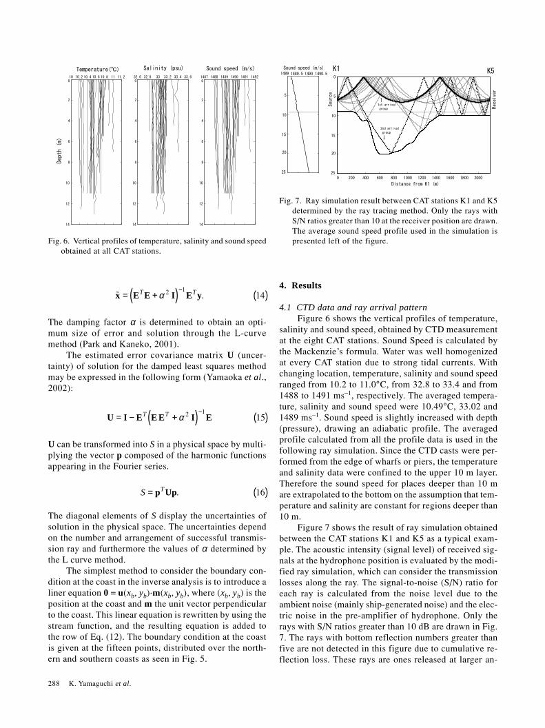
4.1 CTD data and ray arrival patternFigure 6 shows the vertical profiles of temperature,

salinity and sound speed, obtained by CTD measurementat the eight CAT stations. Sound Speed is calculated bythe Mackenzie’s formula. Water was well homogenizedat every CAT station due to strong tidal currents. Withchanging location, temperature, salinity and sound speedranged from 10.2 to 11.0°C, from 32.8 to 33.4 and from1488 to 1491 ms–1, respectively. The averaged tempera-ture, salinity and sound speed were 10.49°C, 33.02 and1489 ms–1. Sound speed is slightly increased with depth(pressure), drawing an adiabatic profile. The averagedprofile calculated from all the profile data is used in thefollowing ray simulation. Since the CTD casts were per-formed from the edge of wharfs or piers, the temperatureand salinity data were confined to the upper 10 m layer.Therefore the sound speed for places deeper than 10 mare extrapolated to the bottom on the assumption that tem-perature and salinity are constant for regions deeper than10 m.

Figure 7 shows the result of ray simulation obtainedbetween the CAT stations K1 and K5 as a typical exam-ple. The acoustic intensity (signal level) of received sig-nals at the hydrophone position is evaluated by the modi-fied ray simulation, which can consider the transmissionlosses along the ray. The signal-to-noise (S/N) ratio foreach ray is calculated from the noise level due to theambient noise (mainly ship-generated noise) and the elec-tric noise in the pre-amplifier of hydrophone. Only therays with S/N ratios greater than 10 dB are drawn in Fig.7. The rays with bottom reflection numbers greater thanfive are not detected in this figure due to cumulative re-flection loss. These rays are ones released at larger an-

Fig. 7. Ray simulation result between CAT stations K1 and K5determined by the ray tracing method. Only the rays withS/N ratios greater than 10 at the receiver position are drawn.The average sound speed profile used in the simulation ispresented left of the figure.Fig. 6. Vertical profiles of temperature, salinity and sound speed

obtained at all CAT stations.


Fig. 8. (a) Stack diagrams of the correlation wave forms ofsignals released from K1 and received at K5 accompaniedby (b) the acoustic intensity and (c) ray travel time calcu-lated at the receiver by the modified ray simulation.

Fig. 9. Hourly mapping of the horizontal current distributionsduring 6:00 to 17:00 of March 18, 2003 obtained by theinverse analysis. CAT stations with successful sound trans-mission are connected with solid lines.

1 m/s

1 m/s

1 m/s

1 m/s

1 m/s

1 m/s

1 m/s

1 m/s

1 m/s

1 m/s

1 m/s 1 m/s

gles from the horizontal at the source position.Reciprocal sound transmission was possible along

all the 16 lines crossing the strait and 2 lines (K5–K7 andK5–K8) on the Moji side. Sound transmission parallel tothe coast was inhibited for the 10 lines due to the pro-truded wharfs and piers. Unfortunately, communicationfailed along the three lines (K4–K6, K4–K7 and K4–K8)related to K4 due to irregular bottom topography aroundK4. Data lacking often occurred due to ship traffic andwas severe, especially for the transmission lines K3–K7and K4–K5. As a result, the number of successful recip-rocal transmission lines reaches 13 to 15.

The correlation wave forms of signals released fromK1 and received at K5 are shown typically in Fig. 8 to-gether with the arrival signal pattern calculated by themodified ray simulation. The tiny effect of current is notconsidered in this ray simulation. The simulated ray ar-rival peaks are located inside the flattened broad peaks inthe real data (Fig. 8(a)), implying that the broad peaksare composed of multi arrival rays (Fig. 8(c)) separatedinto two groups (Fig. 8(b)). The travel time for the typi-cal ray path at the first arrival group (thick solid line)


The 10-minute interval data for travel time are furthersmoothed through a one-hour running mean to reducehigh-frequency variations existing in the strong current.

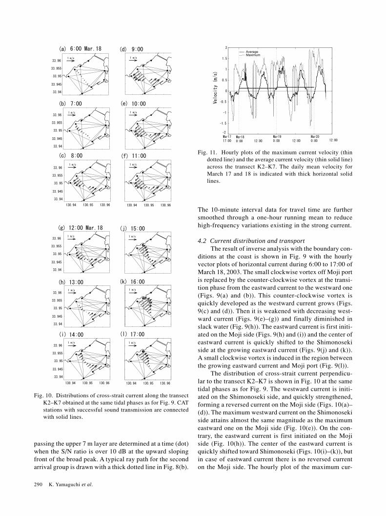
4.2 Current distribution and transportThe result of inverse analysis with the boundary con-

ditions at the coast is shown in Fig. 9 with the hourlyvector plots of horizontal current during 6:00 to 17:00 ofMarch 18, 2003. The small clockwise vortex off Moji portis replaced by the counter-clockwise vortex at the transi-tion phase from the eastward current to the westward one(Figs. 9(a) and (b)). This counter-clockwise vortex isquickly developed as the westward current grows (Figs.9(c) and (d)). Then it is weakened with decreasing west-ward current (Figs. 9(e)–(g)) and finally diminished inslack water (Fig. 9(h)). The eastward current is first initi-ated on the Moji side (Figs. 9(h) and (i)) and the center ofeastward current is quickly shifted to the Shimonosekiside at the growing eastward current (Figs. 9(j) and (k)).A small clockwise vortex is induced in the region betweenthe growing eastward current and Moji port (Fig. 9(l)).

The distribution of cross-strait current perpendicu-lar to the transect K2–K7 is shown in Fig. 10 at the sametidal phases as for Fig. 9. The westward current is initi-ated on the Shimonoseki side, and quickly strengthened,forming a reversed current on the Moji side (Figs. 10(a)–(d)). The maximum westward current on the Shimonosekiside attains almost the same magnitude as the maximumeastward one on the Moji side (Fig. 10(e)). On the con-trary, the eastward current is first initiated on the Mojiside (Fig. 10(h)). The center of the eastward current isquickly shifted toward Shimonoseki (Figs. 10(i)–(k)), butin case of eastward current there is no reversed currenton the Moji side. The hourly plot of the maximum cur-

Fig. 10. Distributions of cross-strait current along the transectK2–K7 obtained at the same tidal phases as for Fig. 9. CATstations with successful sound transmission are connectedwith solid lines.

passing the upper 7 m layer are determined at a time (dot)when the S/N ratio is over 10 dB at the upward slopingfront of the broad peak. A typical ray path for the secondarrival group is drawn with a thick dotted line in Fig. 8(b).

AverageMaximum

Fig. 11. Hourly plots of the maximum current velocity (thindotted line) and the average current velocity (thin solid line)across the transect K2–K7. The daily mean velocity forMarch 17 and 18 is indicated with thick horizontal solidlines.


rent velocity and the average current velocity across thetransect K2–K7 are shown in Fig. 11. The average cur-rent draws a smooth curve with a semidiurnal cycle whilethe maximum current is largely disturbed by the vortex

generation. The average current changes in the range from+1.2 ms–1 (eastward) to –0.5 ms–1 (westward), producingto the upper 7 m transport changes from 13,314 m3s–1 to–5,547 m3s–1. The daily mean transport across the upper

Fig. 12. Time plots of the-range-averaged current velocity calculated along each horizontal transmission line, connecting thepaired CAT stations, before (solid lines) and after (dots) the inverse analysis. The name of station pairs is presented aboveeach time plot.


7 m of the transect is eastward and estimated 1,470m3s–1 for March 18 and 2,140 m3s–1 for March 19, asmarked with thick horizontal lines in Fig. 11.

5. Validation of CAT MeasurementFigure 12 shows the time plots of the range-aver-

aged current velocity calculated along the horizontal trans-mission lines, connecting two CAT stations, before andafter the inverse analysis. The solid curves are the resultsobtained before the inversion and are calculated by sub-stituting the observed travel time difference into the fol-lowing formula (Zheng et al., 1997):

uC

Ltm

m≈ − ( )2

217∆

where Cm is the range averaged sound speed and L thestation-to-station range.

In addition, the hourly rang-averaged current afterthe inversion indicated with dots in the same figure.

The semidiurnal oscillation of current is dominantfor the station pairs K1–K5, K1–K6, K1–K8, K2–K5, K2–K8 and K3–K8 crossing the strait. The current is east-ward over almost the whole tidal period for the stationpairs K5–K7 and K5–K8 located on the Moji side, im-plying the existence of the counter-clockwise vortex offMoji port. The results for the station pairs K1–K5, K1–K6, K2–K5, K2–K6 and K5–K8 show a good agreement

between both results, while the after-inversion resultsunderestimate the peak heights of the before-inversionresults for the station pairs K1–K8, K2–K8, K3–K5 andK3–K8. The spatial interpolation adopted in the inverseanalysis causes this underestimation. The RMS differ-ences for both data are 0.08–0.23 ms–1 for the better groupand 0.32–0.46 ms–1 for the worse one.

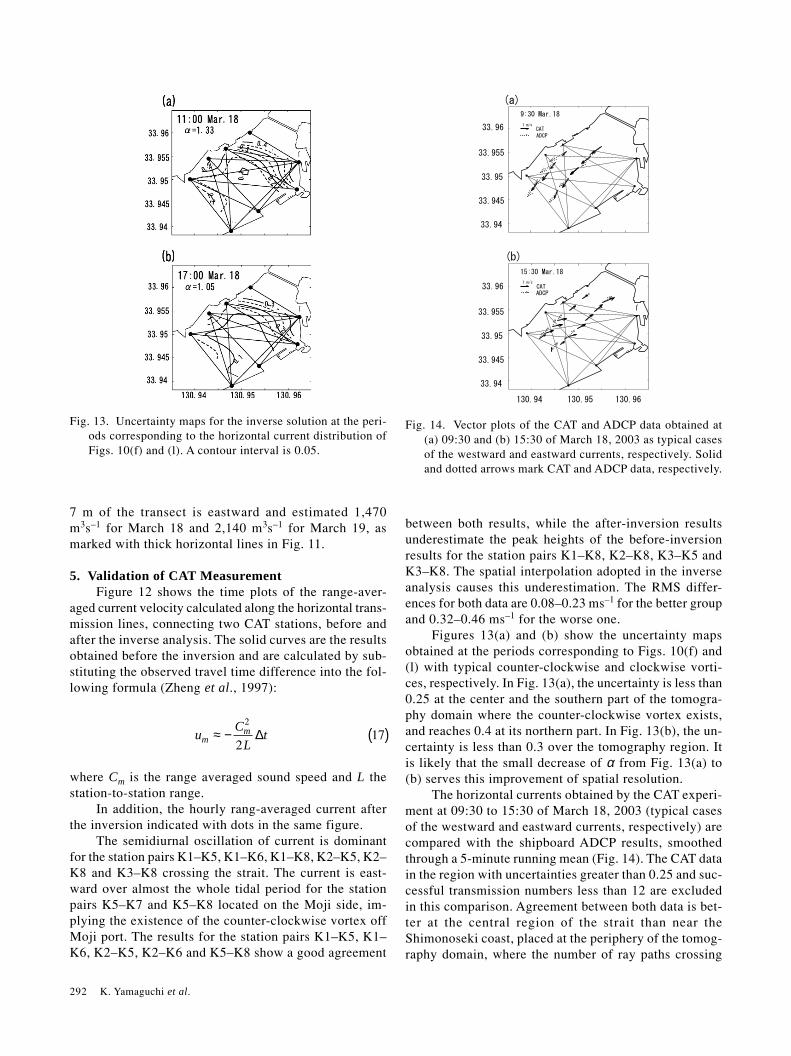
Figures 13(a) and (b) show the uncertainty mapsobtained at the periods corresponding to Figs. 10(f) and(l) with typical counter-clockwise and clockwise vorti-ces, respectively. In Fig. 13(a), the uncertainty is less than0.25 at the center and the southern part of the tomogra-phy domain where the counter-clockwise vortex exists,and reaches 0.4 at its northern part. In Fig. 13(b), the un-certainty is less than 0.3 over the tomography region. Itis likely that the small decrease of α from Fig. 13(a) to(b) serves this improvement of spatial resolution.

The horizontal currents obtained by the CAT experi-ment at 09:30 to 15:30 of March 18, 2003 (typical casesof the westward and eastward currents, respectively) arecompared with the shipboard ADCP results, smoothedthrough a 5-minute running mean (Fig. 14). The CAT datain the region with uncertainties greater than 0.25 and suc-cessful transmission numbers less than 12 are excludedin this comparison. Agreement between both data is bet-ter at the central region of the strait than near theShimonoseki coast, placed at the periphery of the tomog-raphy domain, where the number of ray paths crossing

Fig. 13. Uncertainty maps for the inverse solution at the peri-ods corresponding to the horizontal current distribution ofFigs. 10(f) and (l). A contour interval is 0.05.

Fig. 14. Vector plots of the CAT and ADCP data obtained at(a) 09:30 and (b) 15:30 of March 18, 2003 as typical casesof the westward and eastward currents, respectively. Solidand dotted arrows mark CAT and ADCP data, respectively.


the domain is reduced. The correlation diagram betweenthe CAT and ADCP data is presented in Fig. 15. The cor-relation rates for the east-west current (u) and north-southone (v) are 0.84 and 0.82, respectively. The RMS differ-ence is 0.47 ms–1 for u and 0.48 ms–1 for v. At an overallview, the CAT velocities are considerably smaller thanthe ADCP velocities. This may be caused by the differentaveraging procedure: the average along a ship track isadopted for the ADCP data, while the CAT data are aver-aged through a resolution window on a horizontal plane.

6. SummaryThe horizontal structures of strongly nonlinear tidal

currents generated at the Hayatomono-Seto of the KanmonStrait are mapped on an hourly basis by the coastal acous-tic tomography (CAT) system composed of eight acous-tic stations. The damped least squares method accompa-nied by the L curve method has been applied to recon-struct the vortex-imbedded tidal currents from the traveltime difference data obtained between the paired acous-tic stations, distributed on both the sides of the strait. Themajor features of current structures published in theKanmon Strait Tidal Current Chart of the Japan CoastGuard (1994) such as

1) The large counter-clockwise/small clockwisetidal vortex is induced off Moji port with developing thewestward/eastward current;

2) The maximum tidal currents occur along thenarrow trench near the Shimonoseki coast;

3) The eastward current is first initiated on the Mojiside in the transition phase from the westward to east-ward current;also appear in the mapping charts reconstructed by thepresent inverse analysis. Reconstructed currents are quan-titatively compared with the shipboard ADCP measure-ments. The correlation rates and RMS errors for data se-lected with uncertainty values smaller than 0.25 and trans-mission line numbers larger than 13 are 0.84 and 0.47ms–1 for the east-west current (u) and 0.82 and 0.48 ms–1

for the north-south current (v). The agreement betweenthe CAT and ADCP data is satisfactory regarding themaximum tidal current magnitude reaching 5 ms–1 andthe time resolution of 0.54 ms (one digit width) corre-sponding to the velocity bias of about 0.3 ms–1. As forthe operational system of the Kanmon Strait, the use ofhigher frequency sound of about 20 kHz may be prefer-able to get a velocity accuracy better than 0.1 ms–1.

The daily mean transport for the upper 7 m layeracross the transect K2–K7 is directed eastward and esti-mated 1470 m3s–1 for March 18 and 2140 m3s–1 for March19, 2003 when a spring tide occurs as illustrated in Fig.4. The daily mean eastward transport at the spring tide isstrongly supported by the three-dimensional KanmonStrait model, which is validated with the present CAT andADCP data (Lin et al., 2004).

This CAT experiment demonstrates the ability tomonitor strong tidal current structures in the KanmonStrait.

AcknowledgementsWe are grateful to Ms. Hong Yang and Mr. Kazuhiro

Ito for providing the efficient support in the field experi-ment. Special thanks are to the 7th Regional Coast GuardHeadquarters of the Japan Coast Guard for providingkindly the valuable ADCP observation data. This study issupported by the Grant-in-Aid for the Creation of Inno-vations through Business-Academic-Public Sector Coop-eration of the Japan Ministry of Education, Culture,Sports, Science and Technology.

ReferencesDushaw, B. D. and J. A. Colosi (1998): Ray tracing for ocean

acoustic tomography. Applied Physics Laboratory Report,Univ. Washington, 40 pp.

Fukunishi, M. (1948a): The tidal current in Kanmon Strait (I).J. Japan Soc. Civil Engineers, 33(2), 10–13 (in Japanese).

Fukunishi, M. (1948b): The tidal current in Kanmon Strait (II).J. Japan Soc. Civil Engineers, 33(2), 16–19 (in Japanese).

Japan Coast Guard (1994): Charts of Tidal Currents in theKanmon Strait, 15 pp. (in Japanese).

Jensen, F. B., W. A. Kuperman, M. B. Porter and H. Schmidt(1994): Computational Ocean Acoustics. American Insti-tute of Physics, New York, 612 pp.

Kawano, K. (2000): Tidal current of Kanmon Channel surveyedby acoustic Doppler current profiler and electromagneticflow meter. Tech. Rept. of Shimonoseki Research and Engi-neering Office for Port and Airport, Kyushu Regional De-velopment Bureau, Ministry of Land, Infrastructure andTransport, 4(15), 1–10 (in Japanese).

Lin, J., A. Kaneko, K. Yamaguchi and N. Gohda (2004): A three-dimensional tidal current model of the Kanmon Strait. J.Oceanogr. (submitted).

Munk, W. and C. Wunsch (1979): Ocean acoustic tomography:A scheme for large scale monitoring. Deep-Sea Res., 26,123–161.

Fig. 15. Correlation diagrams between CAT and ADCP data.


Munk, W., P. F. Worcester and C. Wunsch (1995): Ocean Acous-tic Tomography. Cambridge University Press, Cambridge,433 pp.

Park, J.-H. and A. Kaneko (2000): Assimilation of coastal acous-tic tomography data into a barotropic ocean mode. Geophys.Res. Lett., 27, 3373–3376.

Park, J.-H. and A. Kaneko (2001): Computer simulation of thecoastal acoustic tomography by a two-dimensional vortexmode. J. Oceangr., 57, 593–602.

Pierce, A. (1989): Acoustics—An Introduction to Its PhysicalPrinciples and Application. Acoustical Society of America,New York, 678 pp.

Yamaoka, H., A. Kaneko, J.-H. Park, H. Zheng, N. Gohda, T.Takano, X-H. Zhu and Y. Takasugi (2002): Coastal acous-tic tomography system and its field application. IEEE J.Oceanic Eng., 27(2), 283–295.

Zheng, H., N. Gohda, H. Noguchi, T. Ito, H. Yamaoka, T.Tamura, Y. Takasugi and A. Kaneko (1997): Reciprocalsound transmission experiment for current measurement inthe Seto Inland Sea, Japan. J. Oceanogr., 53, 117–127.

Zheng, H., H. Yamaoka, N. Gohoda, H. Noguchi and A. Kaneko(1998): Design of the acoustic tomography system for ve-locity measurement with an application to the coastal sea.J. Acoust. Soc. Japan (E), 19, 199–210.

a continuous mapping of tidal current structures in the ... · ⋅kanmon strait, ⋅coastal...

Documents