a constrained neural network kalman filter for...

International Journal of Neural Systems, Vol. 8, No. 4 (August, 1997) 399–415Special Issue on Data Mining in Financec©World Scientific Publishing Company

A CONSTRAINED NEURAL NETWORK KALMAN FILTERFOR PRICE ESTIMATION IN

HIGH FREQUENCY FINANCIAL DATA

PETER J. BOLLAND∗ and JEROME T. CONNOR†

London Business School, Department of Decision Science,Sussex Place, Regents Park, London NW1 4SA, UK

In this paper we present a neural network extended Kalman filter for modeling noisy financial timeseries. The neural network is employed to estimate the nonlinear dynamics of the extended Kalmanfilter. Conditions for the neural network weight matrix are provided to guarantee the stability of thefilter. The extended Kalman filter presented is designed to filter three types of noise commonly observedin financial data: process noise, measurement noise, and arrival noise. The erratic arrival of data (arrivalnoise) results in the neural network predictions being iterated into the future. Constraining the neuralnetwork to have a fixed point at the origin produces better iterated predictions and more stable results.The performance of constrained and unconstrained neural networks within the extended Kalman filter isdemonstrated on “Quote” tick data from the $/DM exchange rate (1993–1995).

1. Introduction

The study of financial tick data (trade data) is be-

coming increasingly important as the financial in-

dustry trades on shorter and shorter time scales.

Tick data has many problematic features, it is often

heavy tailed (Dacorogna 1995, Butlin and Connor

1996), it is prone to data corruption and outliers

(Chung 1991), and it’s variance is heteroscedastic

with a seasonal pattern within each day (Dacorogna

1995). However the most serious problem with ap-

plying conventional methodologies to tick data is it’s

erratic arrival. The focus of this study is the predic-

tion of erratic time series with neural networks. The

issues of robust prediction and non-stationary vari-

ance are explored in Bolland and Connor (1996a) and

Bolland and Connor (1996b).

There are three distinct types of noise found in

real world time series such as financial tick data:

Process noise represents the shocks that drive the

dynamics of the stochastic process. The distri-

bution of the process/system noise is generally

assumed to be Gaussian. For financial data the

noise distributions can often be heavy tailed.

Measurement noise is the noise encountered when

observing and measuring the time series. The

measurement error is usually assumed to be

Gaussian. The measurement of financial data is

often corrupted by gross outliers.

Arrival noise reflects uncertainty concerning

whether an observation will occur at the next

time step. Foreign exchange quote data is

strongly effected by erratic data arrival. At

times the quotes are missing for forty seconds, at

other times several ticks are contemporaneously

aggregated.

These three types of noise have been widely stud-

ied in the engineering field for the case of a known

deterministic system. The Kalman filter was in-

vented to estimate the state vector of a linear deter-

ministic system in the presence of the process, mea-

surement, and arrival noise. The Kalman filter has

been applied in the field of econometrics for the case

∗E-mail: [email protected]†E-mail: [email protected]

399

400 P. J. Bolland & J. T. Connor

when a deterministic system is unknown and must be

estimated from the data, see for example Engle and

Watson (1987). In Sec. 2, we give a brief description

of the workings of the Kalman filter on linear models.

Neural networks have been successfully applied

to the prediction of time series by many practition-

ers in a diverse range of problem domains (Weigend

1990). In many cases neural networks have been

shown to yield significant performance improvements

over conventional statistical methodologies. Neural

networks have many attractive features compared to

other statistical techniques. They make no para-

metric assumption about the functional relationship

being modeled, they are capable of modeling inter-

action effects and the smoothness of fit is locally

conditioned by the data. Neural networks are gen-

erally designed under careful laboratory conditions

which while taking into consideration process noise,

usually ignore the presence of measurement and ar-

rival noise. In Sec. 3, we show how the extended

Kalman filter can be used with neural network mod-

els to produce reliable predictions in the presence of

process, measurement and arrival noise.

When observations are missing, the neural net-

works predictions are iterated. Because the iterated

feedforward neural network predictions are based on

previous predictions, it acts as a discrete time recur-

rent neural network. The dynamics of the recurrent

network may converge to a stable point; however it

is equally possible that the recurrent network could

oscillate or become chaotic. Section 4 describes a

neural network model which is constrained to have a

stable point at the origin. Conditions are determined

for which the neural network will always converge

to a single fixed point. This is the neural network

analogue of a stable linear system which will always

converge to the fixed point of zero. The constrained

neural network is useful for two reasons:

(1) The extended Kalman filter is guaranteed to

have bounded errors if the neural network

model is observable and controllable (dis-

cussed in Sec. 3). The existence of a stable

fixed point will help make this the case.

(2) It reflects our belief that price increments be-

yond a certain horizon are unpredictable for

the Dollar–DM foreign exchange rates.

For different problems, a neural network with a

fixed point at zero may not make sense, in which

case we do not advocate the constrained neural net-

work. However, for modeling foreign exchange data,

this constrained neural network should yield better

results.In Sec. 5, the performance of the extended

Kalman filter with a constrained neural network is

shown on Dollar–Deutsche Mark foreign exchange

tick data. The performance of the constrained neu-

ral network is shown to be both quantitatively and

qualitatively superior to the unconstrained neural

network.

2. Linear Kalman Filter

Kalman filters originated in the engineering commu-

nity with Kalman and Bucy (1960) and have been ex-

tensively applied to filtering, smoothing and control

problems. The modeling of time series in state space

form has advantages over other techniques both in

interpretability and estimation. The Kalman filter

lies at the heart of state space analysis and provides

the basis for likelihood estimation. The general state

space form for a multivariate time series is expressed

as follows. The observable variables, a n × 1 vector

yt, are related to an m× 1 vector xt, known as the

state vector, via the observation equation,

yt = Htxt + εt t = 1, . . . , N (1)

where Ht is the n × m observation matrix and εt,

which denotes the measurement noise, is a n×1 vec-

tor of serially uncorrelated disturbance terms with

mean zero and covariance matrix Rt. The states are

unobservable and are known to be generated by a

first-order Markov process,

xt = Φtxt−1 + Γtηt t = 1, . . . , N (2)

where Φτ is the m×m state matrix, Γt is an m× gmatrix, and ηt a g × 1 vector of serially uncorre-

lated disturbance terms with mean zero and covari-

ance matrix Qt. A linear AR(p) time series model

can be represented in the general state form by

xt =

φ1 φ2 φ3 · · · φp−1 φp

1 0 0 · · · 0 0

0 1 0 · · · 0 0

0 0 1 0 0...

......

0 0 0 1 0

xt−1 + Γtηt

(3)

A Constrained Neural Network Kalman Filter . . . 401

yt = [1 0 0 · · · 0]xt + εt (4)

where Γt is 1 for the element (1, 1) and zero else-

where. The state space model given by (3) and (4) is

known as the phase canonical form and is not unique

for AR(p) models. There are three other forms which

differ in how the parameters are displayed but all rep-

resentations give equivalent results, see for example

Aoki (1987) or Akaike (1975).

The Kalman filter is a recursive procedure for

computing the optimal estimates of the state vector

at time t, based on the information available at time

t. The Kalman filter enables the estimate of the state

vector to be continually updated as new observations

become available. For linear system equations with

normally distributed disturbance terms the Kalman

filter produces the minimum mean squared error es-

timate of the state xt. The filtering equation written

in the error prediction correction format is,

xt+1|t+1 = xt+1|t + Kt+1yt+1|t (5)

where xt+1|t = Φtxt|t is the predicted state vec-

tor based on information available at time t, Kt+1

is the m × n Kalman gain matrix, and yt+1|t de-

notes the innovations process given by yt+1|t =

yt+1 − Ht+1xt+1|t. The estimate of the state at

t + 1, is produced from the prediction based on in-

formation available at time t, and a correction term

based on the observed prediction error at time t+ 1.

The Kalman gain matrix is specified by the set of

relations,

Kt+1 = Pt+1|tH′t+1[Ht+1Pt+1|tH

′t+1 + Rt+1]−1

(6)

Pt+1|t = Φt+1|tPt|tΦ′t+1|t + Γt+1|tQtΓ

′t+1|t (7)

Pt|t = [I−KtHt]Pt|t−1 (8)

where Pt|t is the filter error covariance. Given the

initial conditions, P0|0 and x0|0, the Kalman filter

gives the optimal estimate of the state vector as each

new observation becomes available.

The parameters of the system of the Kalman

filter, represented by the vector ψ, can be estimated

using maximum likelihood. For the typical system

the parameters, ψ, would consist of the elements of

Qt and Rt, auto-regressive parameters within Φt and

sometimes parameters from within the observation

matrix Ht. The parameters will depend upon the

specific formulation of the system being modeled.

For normally distributed disturbance terms, writ-

ing the likelihood function L(yt; ψ), in terms of the

density of yt conditioned on the information set at

time t− 1, Yt−1 = {yt−1, . . . ,y1}, the log likelihood

function is,

log L=−1

2

N∑t=1

[y′t|t−1ψN−1t|t−1ψ

yt|t−1ψ+ln |Nt|t−1ψ |]

(9)

where yt|t−1ψ is the innovations process and Nt|t−1ψ

is the covariance of that process,

Nt|t−1ψ = HtψPt|t−1ψH′tψ + Rtψ . (10)

The log likelihood function given in (9) depends on

the initial conditions P0|0 and x0|0. de Jong (1989)

showed how the Kalman filter can be augmented to

model the initial conditions as diffuse priors which

allow the initial conditions to be estimated without

filtering implications. After τ time steps, where τ

is specified by the modeller, a proper prior for state

vectors will be estimated and the log likelihood can

then be described as in (9) and (10).

The Kalman filter described is discrete, (as tick

data is quantisized into time steps, i.e. seconds),

however the methodology could be extended to con-

tinuous time problems with the Kalman–Bucy filter

(Meditch 1969).

2.1. Missing data

Irregular (erratic) times series presents a seri-

ous problem to conventional modeling methodolo-

gies. Several methodologies for dealing with erratic

data have been suggested in the literature. Muller

et al. (1990), suggest methods of linear interpolation

between erratic observations to obtain a regular ho-

mogenous times series. Other authors (Ghysels and

Jasiak 1995) have favored nonlinear time deforma-

tion (“business- time” or “tick-time). The Kalman

filter can be simply modified to deal with observa-

tions that are either missing or subject to contempo-

raneous aggregation. The choice of time discretiza-

tion (i.e. seconds, minutes, hours) will depend on

the specific irregular time series. Too small a dis-

cretization and the data set will be composed of

mainly missing observation. Too long a discretiza-

tion and non-synchronous data will be aggregated.

The timing (time-stamp) of financial transactions is


only measured to a precision of one second. A time

discretization of one second is a natural choice for

modeling financial time series as aggregation will be

across synchronous data and missing observations

will be in the minority.

Augmenting the Kalman filter to deal with erratic

time series is achieved by allowing the dimensions of

the observation vector yt and the observation errors

εt, to vary at each time step (nt×1). The observation

equation dimensions now vary with time so,

yt = WtHtxt + εt t = 1, . . . , N (11)

where Wt is an nt × n matrix of fixed weights. This

gives rise to several possible situations:

• Contemporaneous aggregation of the first com-

ponent of the observation vector, in addition to

the other components. So the weight matrix is

((n + 1) × n) and has a row augment for the first

component to give rise to the two values y1t,1 and

y1t,2.

yt =

y1t,1

y1t,2

...

ynt

n+1

,

Wt =

1 0 0 . . . 0

1 0 0 . . . 0

0 1 0 . . . 0

0 0 1 0...

.... . .

0 0 0 1

(n+1)×n

(12)

• All components of the observation equation occur,

where the weight matrix is square (n× n) and an

identity.

yt =

y1t

...

ynt

n

, Wt =

1 . . . 0... 1

...

0 . . . 1

n×n

(13)

• The ith component of the observation vector is un-

observed, so nt is (n − 1) and the weight matrix

(n× (n− 1)) has a single row removed.

yt =

y1t

...

yi−1t

yi+1t

...

ynt

n−1

,

Wt =

0

Ii−1

... 0

...

...

0... In−i0

n×(n−1)

(14)

• All components of the observations vector are un-

observed, nt is zero, and the weight matrix is

undefined.

yt = [NULL], Wt = [NULL] (15)

The dimensions of the innovations yt|t−1ψ , and their

covariance Nt|t−1ψ also vary with nt. Equation (10)

is undefined when nt is zero. When there are no ob-

servations on a given time t, the Kalman filter updat-

ing equations can simply be skipped. The resulting

predictions for the states and filtering error covari-

ance’s are, xt = xt|t−1 and Pt = Pt|t−1. For con-

secutive missing observations (nt = 0, . . . , nt+l = 0)

a multiple step prediction is required, with repeated

substitution into the transition Eq. (2) multiple step

predictions are obtained by

xt+l =

l∏j=1

Φt+j

xt +l−1∑j=1

l∏i=j+1

Φt+i

t

Γt+jηt+j

+ Γt+lηt+l . (16)

The conditional expectations at time t of (16) is given

by

xt+l|t =

l∏j=1

Φt+j

xt (17)

and similarly the expectation of the multiple step

ahead prediction error covariance for the case of time

invariant system is given by

Pt+l|t = ΦlPtΦl +

l−1∑j=0

ΦjΓQ Γ′Φj . (18)


The estimates for multiple step predictions of yt+l|tand xt+l|t can be shown to be the minimum mean

square error estimators Et(yt+l).

2.2. Non-Gaussian Kalman filter

The Gaussian estimation methods outlined above

can produce very poor results in the presence of

gross outliers. The Kalman filter can be adapted

to filter processes where the disturbance terms are

non-Gaussian. The distributions of the process and

measurement noise for the standard Kalman fil-

ter is assumed to be Gaussian. The Kalman fil-

ter can be adapted to filter systems where either

the process or measurement noise is non-Gaussian

(Mazreliez 1973). Mazreliez showed that Kalman fil-

ter update equations are dependent on the distribu-

tion of the innovations and its score function. For a

known distribution the optimal minimum mean vari-

ance estimator can be produced. In the situation

where the distribution is unknown, piecewise linear

methods can employed to approximate it (Kitagawa

1987). Since the filtering equations depends on the

derivative of the distribution, such methods can be

inaccurate. Other methods take advantage of higher

moments of the density functions and require no as-

sumptions about the shape of the probability densi-

ties (Hilands and Thomoploulos 1994). Carlin et al.

(1992), demonstrate the Kalman filter robust to non-

Gaussian state noise. For robustness, heavy tailed

distributions can be consider as a mixture of Gaus-

sians, or an ε-contaminated distribution. If the bulk

of the data behaves in a Gaussian manner then we

can employ a density function which is not domi-

nated by the tails. The Huber function (1980), can

be shown to be the least informative distribution in

the case of ε-contaminated data.In this paper we achieve robustness to measure-

ment outliers by the methodology first described in

Bolland and Connor (1996a). A Huber function is

employed as the score function of the residuals. For

spherically ε-contaminated normal distributions in

R3 the score function g0 for the Huber function is

given by,

g0 = r for r < c

= c for r ≥ c . (19)

The Huber function behaves as a Gaussian for the

center of the distribution and as an exponential in

the tails. The heavy tails will allow the robust

Kalman filter to down weight large residuals and

provide a degree of insurance against the corrupt-

ing influence of outliers. The degree of insurance is

determined by the distribution parameter c in (19).

The parameter can be related to the level of assumed

contamination as shown by Huber (1980).

2.3. Sufficient conditions

For a Kalman filter to estimate the time varying

states of the system given by (1) and (2), the sys-

tem must be both observable and controllable.

An observable system allows the states to be

uniquely estimated from the data. For example,

in the no noise condition (εt = 0) the state xtcan be determined uniquely from future observa-

tions, if the observability matrix given by O =

[H′ Φ′H′ Φ′2H′′ Φ′3H′ · · · ] has Rank(O) =

m where m is the number of elements in the state

vector xt. The condition for observability is also

equivalent to (see Aoki, 1990)

GO =∞∑k=0

(Φ′)kH′HΦk > 0 (20)

where the observability Grammian, GO, satisfies

the following Lyaponov equation, Φ′GOΦ − GO =

−H′H.

The notion of controllability emerged from the

control theory literature where vt denotes an action

that can be made by an operator of a plant. If

the system is controllable, any state can be reached

with the correct sequence of actions. A system Φ

is controllable if the reachability matrix defined by

C = [Γ ΦΓ Φ2Γ Φ3Γ · · · ] has Rank(H) = m

which is equivalent to (see Aoki, 1990)

GC =∞∑k=0

ΦkΓΓ′(Φ′)k > 0 (21)

where the controllability Grammian, GC , satisfies

the following Lyaponov equation, ΦGCΦ′ − GC =

−ΓΓ′.

When a state space model is in one of the four

canonical variate forms such as (3) and (4), the

Grammians GO and GC are identical and the Con-

trollability and Observability requirements are the

same. If Φ is non-singular and the absolute values of

eigenvalues are less than one, the Observability and


Controllability requirements of (20) and (21) will be

met and the Kalman filter will estimate a unique se-

quence of underlying states. In the next two sections

a neural network analogue of the stable linear system

is introduced which will be used within the extended

Kalman filter. If the eigenvalues are greater than

one, the Kalman filter may still estimate a unique

sequence of underlying states but this must be eval-

uated on a system by system basis. See for example

the work by Harvey on the random trend model.

3. Extended Kalman Filter

The Kalman filter can be extended to filter nonlinear

state space models. These models are not generally

conditionally Gaussian and so an approximate filter

is used. The state space model’s observation function

ht(xt) and the state update function ft(xt−1) are no

longer linear functions of the state vector. Using a

Taylor expansion of these nonlinear functions around

the predicted state vector and the filtered state vec-

tor we have,

ht(xt) ≈ ht(xt|t−1) + Ht(xt − xt|t−1)

Ht =∂ht(xt)

∂x′t−1

∣∣∣∣xt=xt|t−1

,(22)

ft(xt−1) ≈ ft(xt−1) + Φt(xt−1 − xt−1)

Φt =∂ft(xt−1)

∂x′t−1

∣∣∣∣xt−1=xt−1

.(23)

The extended Kalman filter (Jazwinski 1970) is pro-

duced by modeling the linearized state space model

using a modified Kalman filter. The linearized ob-

servation equation and state update equation are ap-

proximated by,

yt ≈ Htxt + dt + εt

dt = ht(xt|t−1)− Htxt|t−1

(24)

xt ≈ Φtxt−1 + ct + ηt

ct = ft(xt−1)− Φtxt−1

(25)

and the corresponding Kalman prediction equation

and the state update equation (in prediction error

correction format) are,

xt|t−1 = ft(xt−1)

xt|t = xt|t−1 + Pt|t−1ΦtN−1t [yt − ht(xt|t−1)] .

(26)

The quality of the approximation depends on the

smoothness of the nonlinearity since the extended

Kalman filter is only a first order approximation of

E{xt|Yt−1}. The extended Kalman filter can be

augmented as described in Eqs. (11)–(15) to deal

with missing data and contemporaneous aggregation.

The functional form of ht(xt) and ft(xt−1) are esti-

mated using a neural network described in Sec. 5.

3.1. Sufficient conditions

The nonlinear analog of the AR(p) model expressed

in phase canonical form given by (3) and (4) is ex-

pressed as

xTt = [xt xt−1 xt−2 · · · xt−p+1] (27)

f(xt−1)T = [f(xt−1) xt−1 xt−2 · · · xt−p+1]

(28)

yt = Hf(xt−1)T + εt (29)

with H = [1 0 0 · · · 0] and Γ =

[1 0 0 · · · 0] as in the linear time series model

of (3) and (4).

The Extended Kalman Filter has a long history of

working in practice, but only recently has theory pro-

duced bounds on the resulting error dynamics. Baras

et al. (1988) and Song and Grizzle (1995) have shown

bounds on the EKF error dynamics of determinis-

tic systems in continuous and discrete time respec-

tively. La Scala, Bitmead, and James (1995) have

shown how the error dynamics of an EKF on a gen-

eral nonlinear stochastic discrete time are bounded.

The nonlinear system considered by La Scala et al.

has a linear output map which is also true for our

system described in (27)–(29). As in the case of the

linear Kalman filter, the results of La Scala et al. re-

quire that the nonlinear system be both observable

and controllable.

The nonlinear observability Grammian is more

complicated than its linear counterpart in (21) and

must be evaluated upon the trajectory of interest

(t1 → t2). The nonlinear observability Grammian as

defined by La Scala et al. and applied to the system

given by (27)–(29) is

GO(t, M) =t∑

i=t−MS(i, t)′H′R−1

i H′S(i, t) (30)


where S(t2, t1) = Fy(t2−1)Fy(t2−2) · · ·Fy(t1) and

Fy(t) = ∂f/∂x(y(t)). The nonlinear controllability

Grammian as defined by La Scala et al. and applied

to the system given by (27)–(29) is

GC(t, M) =t−1∑

i=t−MS(t, i+ 1)QiS(t, i+ 1)′ . (31)

As in the linear case of Sec. 2.3, the requirements

that the nonlinear observability and controllability

Grammians given by (30) and (31) are positive are

identical with the appropriate choices of t and M

due to H′R−1i H′ ∼ Q′i. If the Grammians of (30)

and (31) are both positive and finite then the sys-

tem is said to be controllable (observable).

Because of the similarity between observability

and controllability criterions, only the observability

criterion is examined closely. If the observability cri-

terion is positive definite and finite for some values

of M, the system is observable. For the nonlinear

auto-regressive system given by (27)–(29),

Fy(k) =

∂f(y)

∂x1

∂f(y)

∂x2· · · ∂f(y)

∂xp−1

∂f(y)

∂xp

1 0 · · · 0 0

0 1 · · · 0 0...

......

......

0 0 · · · 1 0

.

(32)

The observability Grammian, (30), can be shown to

be finite if S(t+∆, t) converges exponentially to zero.

S(t + ∆, t) will converge exponentially to zero if all

the eigenvalues of Fy(k) are inside the unit circle

for all possible values of y. For any fixed choice of y,

Eq. (32) is equivalent to an AR(p) updating equation

in state space form, this equivalence is easily under-

stood because Fy(k) corresponds to the linearization

of a nonlinear AR(p) model given by (27)–(29). If the

corresponding AR(p) model converges exponentially

to zero for all values of y, then S(t+ ∆, t) will con-

verge exponentially to zero also for this y. An AR(p)

time series model given by wt =∑pi=1 aiwt−i+et will

converge exponentially to zero if all of the zeros of the

polynomial∏pi=1(1 − aiz−1) are inside the unit cir-

cle, see for example Roberts and Mulis (1987). Thus,

the nonlinear autoregressive system, S(t+ ∆, t) will

converge exponentially to zero provided all the roots

of the polynomial given in (33) are inside the unit

circle

g(z) =

p∏i=1

(1− ∂f(y)/∂xi1z−1) . (33)

If in addition, ∂f(y)/∂xi is non-zero, GO is finite

positive definite and there exists an optimal choice

of states which can be estimated with the EKF. In

Sec. 4, conditions are discussed which guarantee the

observability of a neural network system.

The notions of observability and controllablility

are not unique to Kalman filtering. Both notions are

used extensively within control theory. For infor-

mation related to neural networks and control the-

ory, see for example Levin and Narendra (1993) and

Levin and Narendra (1996).

4. Constrained Neural Networks

Often data generating processes have symmetries or

constraints which can be exploited during the esti-

mation of a neural network model. The problem is

how to constrain a neural network to better exploit

these symmetries. One of the key strengths of neural

networks is the ability to approximate any function

to any desired level of accuracy whether the func-

tion has or lacks symmetries, see for example Cy-

benko (1989). In this section a constraint is exam-

ined which is both natural to the financial problems

investigated and desirable from a Kalman filtering

perspective.

A neural network embedded within a Kalman

Filter is used in an iterative fashion in the event of

missing data. As mentioned earlier, linear models

will either diverge if they are unstable or go to zero

if they are stable. In addition, the Kalman Filter

will converge on a unique state sequence if the sys-

tem is stable, if it is unstable the Kalman Filter may

or may not converge on a unique state sequence. It

is thus natural when dealing with linear systems to

want to constrain the system to have stable behavior.

Constraining a linear model to be stable is as sim-

ple as insuring the eigenvalues of the state transition

matrix are between ±1.

For neural networks the dynamics of the system

can exhibit complicated behavior where the state tra-

jectories can be cyclical, chaotic, or converge to one

of multiple fixed point attractors. For the problems

we are interested in, a limiting point of zero is de-

sirable. From the perspective of a Kalman filter, the


system is stable. From view of the financial exam-

ple presented later, a limiting point of zero will cor-

respond to future price increments being unknown

beyond a certain distance into the future.

There are two ways of putting symmetry con-

straints in neural networks, a hard symmetry con-

straint obtained by direct embedding of the symme-

try in the weight space and a soft constraint of push-

ing a neural network towards a symmetric solution

but not enforcing the final solution to be symmetric.

The soft constraint of biasing towards symmet-

ric solutions can be viewed from two perspectives,

providing hints and regularization. Abu-Mostafa

(1990), (1993), and (1995), showed among other

things that it is possible to augment a data set with

examples obtained by generating new data under the

symmetry constraint. The neural network is then

trained on the augmented training set and is likely

to have a solution that is closer to the desired sym-

metric solution then would otherwise be the case.

The soft constraint can come in the form of extra

data generated from a constraint or as a constraint

within the learning algorithm itself. Alternatively,

neural networks which drift from the symmetric so-

lution can be penalized by a regularization term, see

for example the tangent prop by Simard, Victorri,

La Cunn, and Denker (1992). Both the hint and

the regularization approach to soft constraints were

shown to be related by Leen (1995).

The alternative of hard constraints was first

proposed by Giles et al. (1990) in which a neural

network was made invariant under geometric trans-

formations of the input space. We propose to incor-

porate a hard constraint in which a neural network is

forced to have a fixed point at the origin, producing

a forecast of zero when past observations, yt−i for

i = 1, . . . , p are equal to zero.

The imposition of a fixed point in the neural net-

work will have the largest effect when the predic-

tor is being iterated. The iterated predictor is, as

will be described in Sec. 4.1, a recurrent neural net-

work. A fixed point need not alter the estimated

neural network significantly. Jin et al. (1994) show

there must be at least one fixed point in a recurrent

network anyway. As the example in Sec. 5 demon-

strates, an unconstrained iterated predictor will

often converge to a fixed point in any case, the prob-

lem is that the resulting fixed point is found to be

undesirable.

Other possible dangers exist with recurrent neu-

ral networks. The existence of a fixed point does not

preclude chaos, the fixed point may be unstable or

only stable locally. Often recurrent neural networks

can perform oscillations or more complicated types

of stable or chaotic patterns, see for example Marcus

and Westervelt (1989), Pearlmutter (1989), Pineda

(1989), Cohen (1992), Blum and Wang (1992) and

many others. Under some circumstances this com-

plicated behavior in an iterated predictor could be

desirable, however it is the view of this paper that

any advantages are outweighed by the dangers of us-

ing a Kalman filter on a poorly understood nonstable

system.

A fixed point at yt = 0 is achieved by augmenting

a neural network with a constrained output bias pa-

rameter. For a network consisting of H hidden units

and with activation function f, the functional form

of the constrained network is given by,

yt =H∑i=1

Wif

p∑j=1

wijyt−j + θi

−

H∑i=1

Wif(θi) . (34)

where parameters of the network Wi, wij , and θi,

represent the output weights, input weights and the

input biases. The first term of (34) describes a

standard feedforward neural network and the second

term represents the “hard wired” constraint. Con-

ditions which will ensure that the fixed point is a

stable attractor will be discussed in Sec. 4.2. The

fixed point will only be guaranteed to be a local at-

tractor. Outside of the local area surrounding the

origin, the behavior of the neural network model will

be determined by the data used for training.

The estimation of the parameters can be achieved

by using a slightly augmented back-propagation al-

gorithm. For a mean squared error cost function

the fixed point constraint leads to a slightly more

complicated learning rule based on the following

derivatives,

dyt

dWi= f

p∑j=1

wijyt−j + θi

− f(θi) (35)


dyt

dθi= Wif

p∑j=1

wijyt−j + θi

×

1− f

p∑j=1

wijyt−j + θi

− Wif(θi)(1− f(θi)) (36)

with the derivative of the prediction w.r.t. the in-

puts, dyt/dwik, being unaffected by the constraint

on the neural network. The neural network train-

ing algorithm assumes that the initial weight matrix

satisfies the fixed point constraint.

4.1. Iterated behavior of neural

network

The neural network in (34) is a simple feedforward

neural network with no feedback connections. As the

neural network stops receiving new data and begins

running in an iterated manner, the neural network

predictions will be based on past neural network pre-

dictions

xt = fNN(xt−1, . . . , xt−k, xt−k−1, . . . , xt−p) . (37)

Recurrent connections are implicitly being added

when the neural network is running iteratively within

the Extended Kalman filtering system. After p time

steps have been processed without receiving any

data, the system is no longer receiving data from

outside the system. The iterated system is as de-

picted in Fig. 1. The recurrent activations of the

neural units can be divided into three sets; the ac-

tivations of the hidden units, si for 1 ≤ i ≤ H; the

activation of the output unit, sH+1 for i = H + 1;

the activation of the input units, sH+I for H + 2 ≤i ≤ H + p.

si(t+ 1) = f

θi +

p∑j=1

wijsH+j(t)

, 1 ≤ i ≤ H

(38)

s(H+1)(t+ 1) =H∑j=1

Wjsj(t) , i = H + 1 (39)

sH+i(t+ 1) = sH+i−1(t) H + 2 ≤ i ≤ H + p

(40)

Fig. 1. Iterated neural network.

where the parameters W and w are identical to

the system given by (34). The recurrent neu-

ral network is different from the feedforward neu-

ral network because of the addition of p neurons,

sH+1(t), . . . , sH+p(t), which enable the previous pre-

dictions to be stored in the system via (39) and (40)

and used as a basis for further predictions. The re-

sulting recurrent connections are much more limited

than considered in most recurrent network studies.

Whether the behavior of the recurrent network

given by (38)–(40) is stable, oscillatory or chaotic is

determined by the weights. The next section will

state under what conditions the neural network will

converge to a fixed point.

4.2. Absolute stability of discrete

recurrent neural networks

The strongest results on the stability of recurrent

networks are for the continuous time versions. The

popular Hopfield network (Hopfield 1984) is guar-

anteed to be stable because the weight matrix is

confined to be symmetric. The convergence of non-

symmetric recurrent neural networks in continuous

time has been investigated by Kelly (1990) and oth-

ers. Matsuoka (1992) in particular has shown how

weights of a non-symmetric recurrent neural network

can be extremely large and convergence can still be

guaranteed in some cases.

The guarantees for convergence of discrete time

recurrent networks are not as strong as that of


continuous time neural networks. Many weight

configurations which lead to convergence in continu-

ous time neural networks do not produce convergence

for the case of discrete time recurrent networks.

For a discrete time recurrent network to be ab-

solutely stable, it must converge to a fixed point in-

dependent of the initial starting conditions. Results

of Jin et al. (1994) for fully recurrent networks will

be reviewed. These results will be applied to the

special case of the constrained network. Jin et al.

(1994) reported that a fully recurrent network of the

form

si(t+ 1) = f

θi +H∑j=1

ωijsj(t)

i = 1, . . . , H

(41)

will converge to a fixed point if all of the eigenvalues

of the matrix W of network weights ωij fall within

the unit circle. Jin et al. then generalize the results

by noting that the eigenvalues are not change by the

transformation P−1WP when is a non-singular ma-

trix of equivalent dimensions. Jin et al. consider the

transformation P = diag(p1, . . . , pN ) where pi are all

positive which leads to leads to following guarantee

of stability

|ωii|+1

p2γ−1i

(Rpi )γ(Cpi )1−γ < c−1i (42)

with ci denoting the maximum slope of the ith non-

linear neuron transfer function, γ ∈ [0, 1], Rpi and

Cpi are given by

Rpi =∑j 6=i

pj |ωij | , (43)

Cpi =∑j 6=i

1

pj|ωji| (44)

and (p1, . . . , pn) are all positive.

4.2.1. The general case

Stability guarantees for neural networks using (41)

are typically quoted for two cases, γ = 0 and γ = 1.

The fully recurrent network given by (41) is more

general than the iterated neural network given in

(38)–(40). For the iterated neural network, the sta-

bility guarantees (38) reduces to the following two

cases.

With a choice of γ = 0:

pi

pH+1|Wi| < c−1

i , i = 1, . . . , H (45)

pi

1

pi+1+

H∑j=1

|wj,i−H |pj

< 1,

i = H + 1, . . . , H − p− 1 (46)

pi

H∑j=1

|wj,i−H |pj

< 1, i = H + p (47)

This is equivalent to a weighted sum of the absolute

value of the weights leaving each neuron multiplied

by the maximum slope of a neuron nonlinearity being

less than one.With a choice of γ = 1.

1

pi

p∑j=1

pH+j |wij | < c−1i i = 1, . . . , H (48)

1

pH+1

H∑j=1

pj |Wj | < 1 i = H + 1 (49)

pi−1

pi< 1 i = H + 2, . . . , H + p .

(50)

This is equivalent to a weighted sum of the abso-

lute value of the weights going entering each neuron

multiplied by the maximum slope of a neuron non-

linearity being less than one.Any choice of positive (p1, . . . , pn) is allowable,

two natural choices for the iterated neural network

are now listed.

4.2.2. All pi equal

The choice of p = (p0, p0, . . . , p0) will not satisfy

(45)–(47) or (48)–(50) because of the recurrent con-

nections which are equal to 1. However, if pi = p0 +

(i−H − 1)ε is used instead for i = H + 2, . . . , H + p

where ε is vanishingly small, the stability guarantees

of (48)–(50) reduce to

p∑j=1

|wij | < c−1i , i = 1, . . . , H , (51)

H∑j=1

|Wj | < 1, i = H + 1 . (52)


Equations (45)–(47) do not have an equally parsimo-

nious expression for the pi being equal case.

4.2.3. Scale invariance

A transformation which will not alter the recurrent

network is obtained by taking advantage of its au-

toregressive structure. The output of the network

can be scaled as long as the weights connected to

past predictions are divided by the same constant,

this leads to a network with equivalent dynamics

and weights given by W ′i = kWi and w′ij = k−1wij .

The guarantee for stability given by (51) and (52)

becomes

p∑j=1

|wij | < kc−1i , i = 1, . . . , H , (53)

H∑j=1

|Wj | < k−1, i = H + 1 . (54)

Equations (51) and (52) can easily be optimized by

choosing k−1 = ΣHj=1|Wj | + ε with ε being vanish-

ingly small and positive and checking that (51) still

holds.

4.3. The relationship between absolute

stability and observability

In Sec. 3 the extended Kalman filter was said to be

observable if the eigenvalues of the transition matrix

were inside the unit circle. The stability results of

the constrained neural network presented in Sec. 4.1

are equivalent to guaranteeing the roots of the poly-

nomial g(z) given in (33) are inside the unit circle.

In addition, if (32) is invertible, a constrained neural

network will be observable.

4.4. Stability of the constrained

neural network

When the constrained neural network given in (34)

is iterated it is the same form as the iterated neural

network given in (38)–(40), with the exception of a

bias term. Bias terms have no effect on the stability

of an iterated constrained neural network, hence the

above stability arguments apply also to the stability

of the constrained neural network.

5. Application to “Tick” Data

The financial institutions are continually striving for

a competitive edge. With the increase in computer

power and the advent of computer trading, the finan-

cial markets have dramatically increased in speed.

Technology is creating new trading horizons which

give access to possible inefficiencies of the market.

The volume of trading has increased hugely and the

price series (tick data) of these trades offers a great

source of information about the dynamics of the mar-

kets and the behavior of its practitioners. A ma-

jor problem for financial institutions that trade at

high frequency is estimating the true value of the

commodity being traded at the instance of a trade.

This problem is faced by both sides of transaction,

the market maker and the investor. The uncertainty

arises from many sources. There are several sources

of additive noise. The state noise dominates, how-

ever bid ask bounce, price quantization, and typo-

graphic errors result in observation noise. In addi-

tion to these uncertainties the estimate of the value

has to be based on information that may be several

time periods old. The methodology we present ad-

dresses these problems and produces an estimate of

the “true mid-price” irrespective of the data’s erratic

nature.

The Dollar/Deutsche Mark exchange rates were

modeled. The data was obtained from Reuters

FXFX pages, and covered the period March 1993–

April 1995. As the data is composed of only quotes

then the possible sources of noise are amplified.

Compared to brokers data or actual transactions

data the quality of quote data is very poor. The

price spreads (bid/ask) are larger, the data is prone

to miss-typing error and also some of the quotes are

simply advertisements for the market makers. In

general quotation have more process noise and more

sources of measurement noise. However quotation

data is readily available and the most liquid and ac-

cessible view of the market.

To eliminate some of the bid-ask noise in the se-

ries, the changes in the mid-price were modeled. The

filtered states represent the estimated “true” mid-

prices. For an NAR(p) model the one step ahead

prediction is,

xt+1|t = f(xt) = xt + g(xt − xt−1, . . . , xt−p+1 − xt−p)

(55)


where g is the predicted change in state based on

the changes in previous time periods. The func-

tion g was estimated by both a constrained feed-

forward neural network and an unconstrained neu-

ral network. For the results shown here a simple

NAR(1) model was estimated. A parsimonious neu-

ral network specification was used, with a 4 hidden

unit feed forward network using sigmoidal activation

functions.

An estimation maximization (EM) algorithm is

employed at the center of a robust estimation pro-

cedure based on filtered data (for full details see

Bolland and Connor 1996). The EM algorithm, see

Dempster, Laird, and Rubin (1977), is the standard

approach when estimating model parameters with

missing data. The EM algorithm has been used in

the neural network community before, see for ex-

ample Jordan and Jacobs (1993) or Connor, Mar-

tin, and Atlas (1994). During the estimation step,

the missing data, namely the xt, εt, and ηt of (1)

and (2) must be estimated. This amounts to esti-

mating parameters of the state update function f

and the noise variance matrices Qt and Rt. With

the estimated missing data assumed to be true, the

parameters are then chosen by way of maximizing

the likelihood. This procedure is iterative with new

parameter estimates giving rise to new estimates of

missing data which in turn give rise to newer pa-

rameter estimates. The iterative estimation proce-

dure was initialized by constructing a contiguous

data set (no arrival noise) and estimating a linear

auto-regressive model. The variances of the distur-

bance terms are non-stationary. To remove some of

this non-stationarity the intra day seasonal pattern

of the variances were estimated (Bolland and Connor

1996). The parameters of the state update function

were assumed to be stationary across the length of

the data set.

Table 1. Non-iterated forecasts.

Fig. 2. Estimated function.


Fig. 3. Estimated function at origin.

Fig. 4. Filtered tick data.

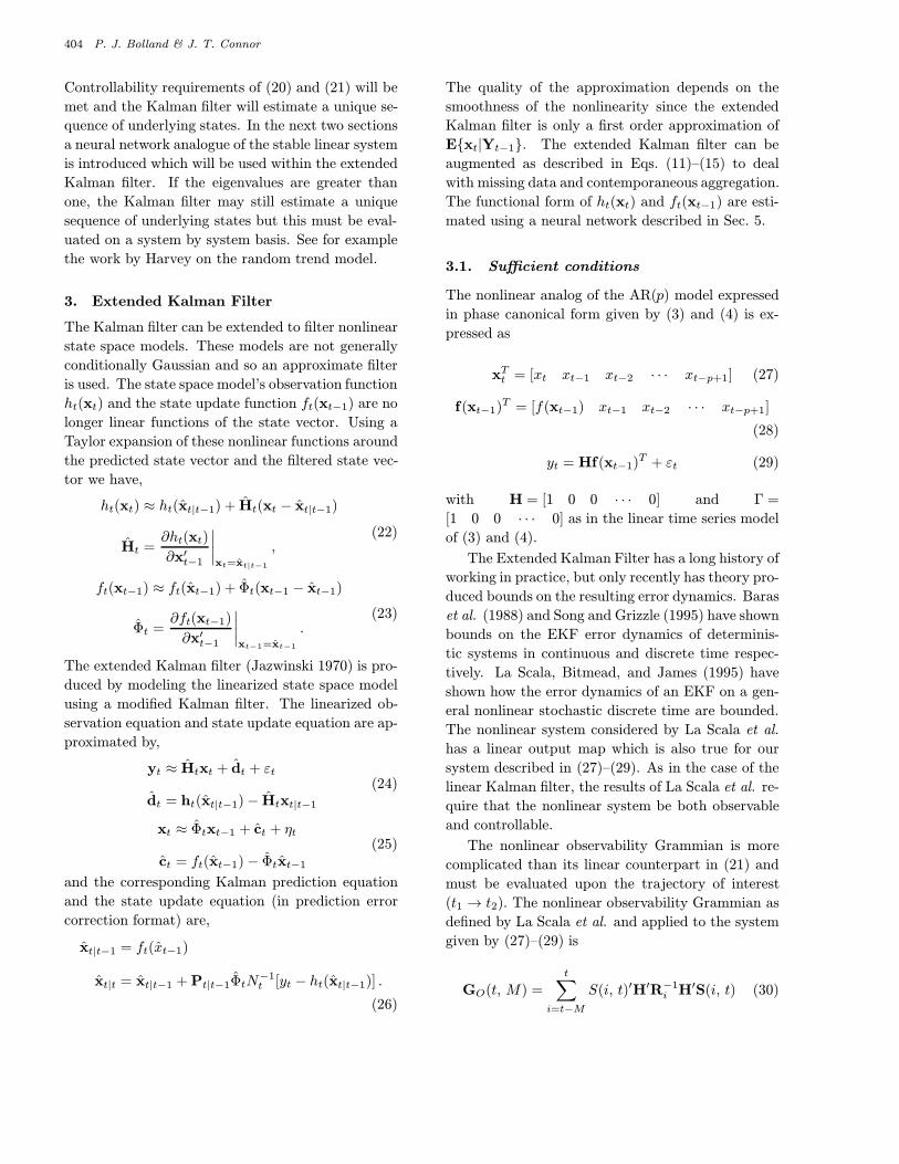
Table 1 gives the performance of the two modelsfor non-iterated forecast. The constraints on the net-work are not detrimental to the overall performance,with the percentage variance explained (r-squared)and the correlation being very similar.

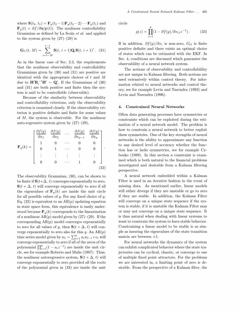
Figure 2 shows the fitted function of a simpleNAR(1) model for the constrained neural network

and the unconstrained neural network. The qualita-tive difference in the models estimated function areonly slight.

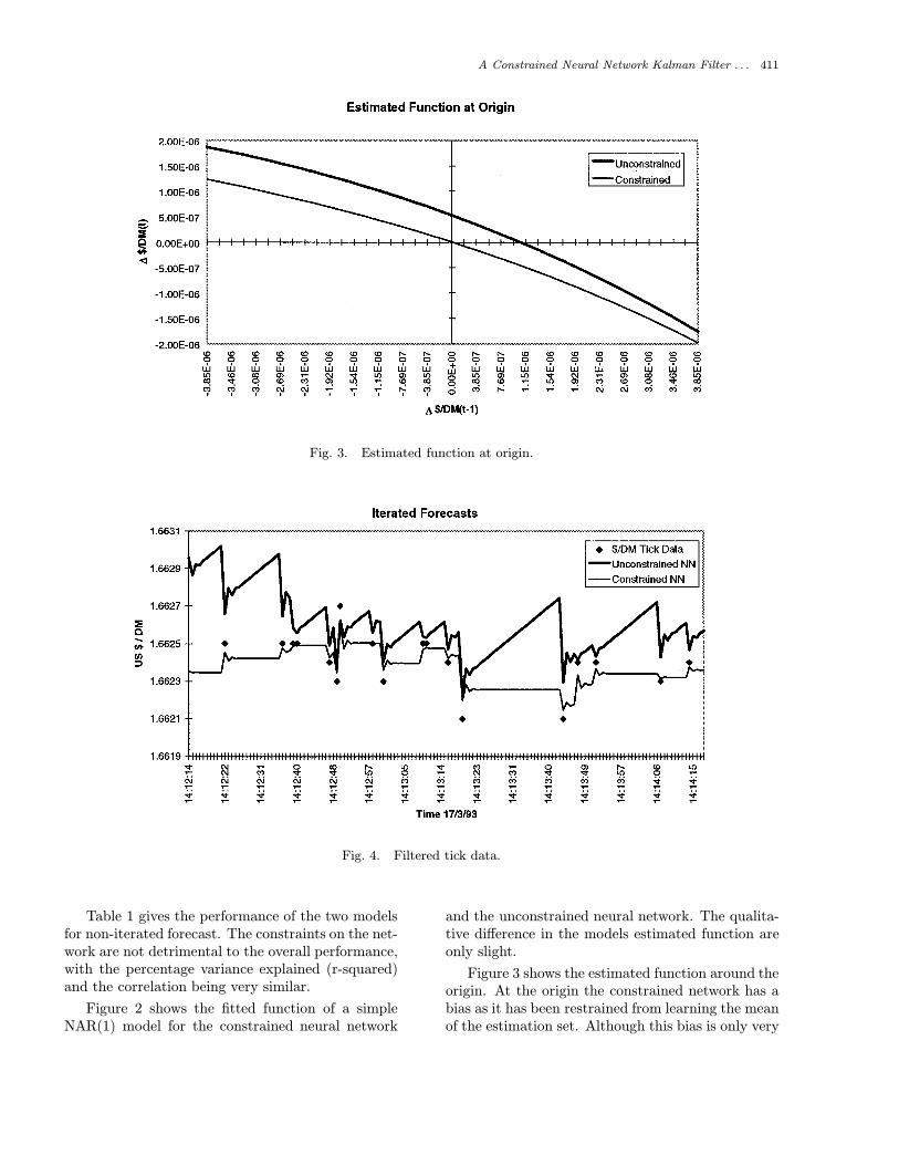
Figure 3 shows the estimated function around theorigin. At the origin the constrained network has abias as it has been restrained from learning the meanof the estimation set. Although this bias is only very


Fig. 5. Stable points of network.

Table 2. Test set performance.

Fig. 6. Iterated forecast error.


small (for linear regression the bias is 5.12 × 10−7

with a t-statistic of 0.872), its effect large as it iscompounded by iterating the forecast.

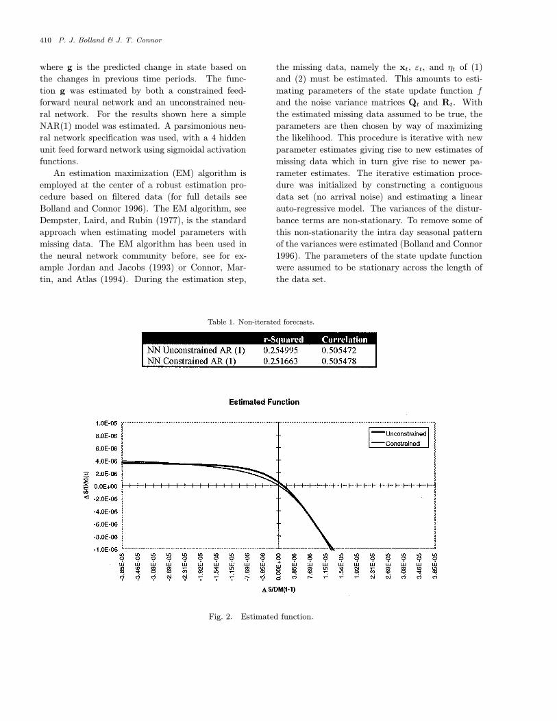
The filter produces estimated states (shown inFig. 4) which can be viewed as the “true mid-prices,” the noise due to market friction’s has beenestimated and filtered (bid-ask bounce, price quan-tization, etc.). The iterated forecasts reach thestable point after only small number of iterations(approx. 5).

Figure 5 shows a close up of the iterated forecastsof the two networks. The value of the stable pointin the case of the simple NAR(1) is the final gra-dient of the iterated forecasts. The stable point ofthe constrained neural network is zero, and the sta-ble point of unconstrained is 1.57× 10−6. This is theresult of a small bias in the model. When the fore-cast is iterated this bias is accumulated and thereforethe unconstrained network predictions trend. Forthe constrained network the iterated forecast soonreach the stable point zero, reflecting our prior be-lief in the long term predictability of the series. Themean squared error (MSE) as well as the medianabsolute deviations (MAD) of the constrained andunconstrained networks are given in Table 2, andshown in Fig. 6. As the forecast is iterated the MSEfor the unconstrained grows rapidly. This is due toits trending forecast.

It is clear that the performance is improved byconstraining the neural network. The MSE for theconstrained neural network remains relatively con-stant with prediction. The accuracy of iterated pre-diction should decrease as the forecast is iterated.From Fig. 6 it is clear that the MSE is not increasingwith number of iterations. However, only in periodsof very low trading activity are forecasts iterated for40 time steps also in periods of low trading activitythe variance in the time series is low. So the errorsin these periods are only small even though the timebetween observations can be large.

6. Conclusion and Discussion

Using neural networks within an extended Kalmanfilter is desirable because of the measurement andarrival noise associated with foreign exchange tickdata. The desirability of using a stable system withina Kalman filter was used as an analogy for develop-ing a “stable neural network” for use within an ex-tended Kalman filter. The “stable neural network”was obtained by constraining the neural network tohave a fixed point of zero input gives zero output. Inaddition, the fixed point at zero reflected our belief

that price increments beyond a certain horizon areunknowable and a predicted price increment of zerois best (random walk). This constrained neural net-work is optimized for foreign exchange modeling, forother problems a constrained neural network with afixed point at zero would be undesirable.

The behavior of the neural network within the ex-tended Kalman filter under normal operating condi-tions is roughly the same as the unconstrained neuralnetwork. But in the presence of missing data, the it-erated predictions of the constrained neural networkfar outperformed the unconstrained neural networkin both quality and performance metrics.

References

Y. S. Abu-Mostafa 1990, “Learning from hints in neuralnetworks,” J. Complexity 6, 192-198.

Y. S. Abu-Mostafa 1993, “A method for learning fromhints,” Advances in Neural Information Processing 5,ed. S. J. Hanson (Morgan Kaufmann), pp. 73–80.

Y. S. Abu-Mostafa 1995, “Financial applications of learn-ing from hints,” Advances in Neural Information Pro-cessing 7, eds. J. Tesauro, D. S. Touretzky and T.Leen (Morgan Kaufman), pp. 411–418.

H. Akaike 1975, “Markovian representation of stochasticprocesses by stochastic variables,” SIAM J. Control13, 162–173.

M. Aoki 1987, State Space Modeling of Time Series,Second Edition (Springer–Verlag).

J. S. Baras, A. Bensoussan and M. R. James 1988,“Dynamic observers as asymptotic limits of recur-sive filters: Special cases,” SIAM J. Appl. Math. 48,1147–1158.

E. K. Blum and X. Wang 1992, “Stability of fixed pointsand periodic orbits and bifurcations in analog neuralnetworks,” Neural Networks 5, 577–587.

P. J. Bolland and J. T. Connor 1996, “A robust non-linearmultivariate Kalman filter for arbitrage identificationin high frequency data,” in Neural Networks in Fi-nancial Engineering (Proceedings of the NNCM-95),eds. A-P. N. Refenes, Y. Abu-Mostafa, J. Moody andA. S. Weigend (World Scientific), pp. 122–135.

P. J. Bolland and J. T. Connor 1996b, “Estimationof intra day seasonal variances,” Technical Report,London Business School.

S. J. Butlin and J. T. Connor 1996, “Forecastingforeign exchange rates: Bayesian model compari-son using Gaussian and Laplacian noise models,”in Neural Networks in Financial Engineering (Proc.NNCM-95), eds. A.-P. N. Refenes, Y. Abu-Mostafa, J.Moody and A. Weigend (World Scientific, Singapore),pp. 146–156.

B. P. Carlin, N. G. Polson and D. S. Stoffer 1992, “AMonte Carlo approach to nonnormal and nonlin-ear state-space modeling,” J. Am. Stat. Assoc. 87,493–500.


P. Y. Chung 1991, “A transactions data test of stockindex futures market efficiency and index arbitrageprofitability,” J. Finance 46, 1791–1809.

M. A. Cohen 1992, “The construction of arbitrary sta-ble dynamics in nonlinear neural networks,” NeuralNetworks 5, 83–103.

J. T. Connor, R. D. Martin and L. E. Atlas 1994,“Recurrent neural networks and robust time se-ries prediction,” IEEE Trans. Neural Networks4, 240–254.

G. Cybenko 1989, “Approximation by superpositions ofa sigmoidal function,” Math. Control, Signals Syst. 2,303–314.

M. M. Dacorogna 1995, “Price behavior and models forhigh frequency data in finance,” Tutorial, NNCM con-ference, London, England, Oct, pp. 11–13.

P. de Jong 1989, “The likelihood for a state space model,”Biometrica 75, 165–169.

A. P. Dempster, N. M. Laird and D. B. Rubin 1977,“Maximum likelihood from incomplete data via theEM algorithm,” J. Royal Stat. Soc. B39, 1–38.

R. F. Engle and M. W. Watson 1987, “The Kalman filter:Applications to forecasting and rational expectationmodels,” in Advances in Econometrics Fifth WorldCongress, Volume I, ed. T. F. Bewley (CambridgeUniversity Press).

E. Ghysels and J. Jasiak 1995, “Stochastic volatility andtime deformation: An application of trading volumeand leverage effects,” Proc. HFDF-I Conf., Zurich,Switzerland, March 29–31, Vol. 1, pp. 1–14.

C. L. Giles, R. D. Griffen and T. Maxwell 1990, “En-coding geometric invariance’s in higher order neuralnetworks,” in Neural Information Processing Systems,ed. D. Z. Anderson (American Institute of Physics),pp. 301–309.

A. V. M. Herz, Z. Li and J. Leo van Hemmen, “Statisticalmechanics of temporal association in neural networkswith delayed interactions,” NIPS, 176–182.

T. W. Hilands and S. C. Thomoploulos 1994, “High-orderfilters for estimation in non-Gaussian noise,” Inf. Sci.80, 149–179.

J. J. Hopfield 1984, “Neurons with graded responsehave collective computational properties like thoseof two-state neurons,” Proc. Natl. Acad. Sci. 81,3088–3092.

P. J. Huber 1980, Robust Statistics (Wiley, New York).A. H. Jazwinshki 1970, Stochastic Processes and Filtering

Theory (Academic Press, New York).L. Jin, P. N. Nikiforuk and M. Gupta 1994, “Absolute

stability conditions for discrete-time recurrent neu-ral networks,” IEEE Trans. Neural Networks 5(6),954–64.

M. I. Jordan and R. A. Jacobs 1992, “Hierarchical mix-tures of experts and the EM algorithm,” Neural Com-put. 4, 448–472.

R. E. Kalman and R. S. Bucy 1961, “New results in lin-ear filtering and prediction theory,” Trans. ASME J.Basic Eng. Series D 83, 95–108.

D. G. Kelly 1990, “Stability in contractive nonlinearneural networks,” IEEE Trans. Biomed. Eng. 37,231–242.

G. Kitagawa 1987, “Non-Gaussian state-space modelingof non-stationary time series,” J. Am. Stat. Assoc.82, 1033–1063.

B. F. La Scala, R. R. Bitmead and M. R. James 1995,“Conditions for stability of the extended kalman fil-ter and their application to the frequency trackingproblem,” Math. Control Signals Syst. 8, 1–26.

Y. Le Cun, B. Boser, J. S. Denker, D. Henderson, R. E.Howard, W. Hubbard and L. D. Jackel 1990, “Hand-written digit recognition with a back-propagation net-work,” in Advances in Neural Information ProcessingSystems 2, ed. D. S. Touretzky (Morgan Kaufmann),pp. 396–404.

T. K. Leen 1995, “From data distributions to reg-ularization in invariant learning,” in Advances inNeural Information Processing 7, eds. J. Tesauro,D. S. Touretzky and T. Leen (Morgan Kaufman),pp. 223–230.

A. U. Levin and K. S. Narendra 1996, “Control of nonlin-ear dynamical systems using neural networks — PartII: Observability, identification, and control,” IEEETrans. Neural Networks 7(1).

A. U. Levin and K. S. Narendra 1993, “Control of nonlin-ear dynamical systems using neural networks: Con-trollability and stabilization,” IEEE Trans. NeuralNetworks 4(2).

C. M. Marcus and R. M. Westervelt 1989, “Dynam-ics of analog neural networks with time delay,” Ad-vances in Neural Information Processing Systems 2,ed. D. S. Touretzky (Morgan Kaufmann).

C. J. Mazreliez 1973, “Approximate non-Gaussian filter-ing with linear state and observation relations,” IEEETrans. Automatic Control, February.

K. Matsuoka 1992, “Stability Conditions for nonlinearcontinuous neural networks with asymmetric connec-tion weights,” Neural Networks 5, 495–500.

J. S. Meditch 1969, Stochastic Optimal Linear Estimationand Control (McGraw-Hill, New York).

U. A. Muller, M. M. Dacorogna, R. B. Oslen, O. V.Pictet, M. Schwarz and C. Morgenegg 1990, “Statisti-cal study of foreign exchange rates, empirical evidenceof a price change scaling law, and intraday analysis,”J. Banking and Finance 14, 1189–1208.

B. A. Pearlmutter 1989, “Learning state-space trajecto-ries in recurrent neural networks,” Neural Computa-tion 1, 263–269.

F. J. Pineda 1989, “Recurrent backpropagation and thedynamical approach to adaptive neural computa-tion,” Neural Computation 1, 161–172.

R. Roll 1984, “A simple implicit measure of the effectivebid-ask spread in an efficient market,” J. Finance 39,1127–1140.

P. Simard, B. Victorri, Y. La Cunn and J. Denker 1992,“Tangent prop- a formalism for specifying selectivevariances in an adaptive network,” in Advances in


Neural Information Processing 4, eds. J. E. Moody,S. J. Hanson and R. P. Lippman (Morgan Kaufman),pp. 895–903.

Y. Song and J. W. Grizzle 1995, “The extended Kalmanfilter as a local observer for nonlinear discrete-timesystems,” J. Math. Syst. Estim. Control 5, 59–78.

A. S. Weigend, B. A. Huberman and D. E. Rumel-hart 1990, “Predicting the future: A connectionist ap-proach,” Int. J. Neural Systems 1, 193–209.

a constrained neural network kalman filter for...

Documents