a conceptual spatial system dynamics (ssd) model for ...mssanz.org.au/modsim2013/b2/neuwirth.pdf ·...

A conceptual spatial system dynamics (SSD) model for structural changes in grassland farming

C. Neuwirtha and A. Peckb

a Doctoral College GIScience, University of Salzburg, Salzburg, Austria Email: [email protected]

b Department of Civil and Environmental Engineering, University of Western Ontario, London, Canada

Abstract: Typically, discrete-time agent-based models and cellular automata approaches have been used to model farm structural changes. However, the proposed methodology uniquely considers a cross-disciplinary, continuous System Dynamics (SD) simulation approach to capture temporal dynamics of grasslands farming structure. The SD approach is particularly well suited for participatory modeling and involving stakeholders in the model development and simulation processes.

In order to capture both spatial and temporal dimensions, this paper proposes a Spatial System Dynamics (SSD) approach. This approach is based on the strengths of system dynamics theory and geographical spatial modeling tools. The SSD approach links system dynamics (temporal simulation) and GIS (spatial analysis and visualization) software. For the purpose of this research, farm structural change is defined by the dynamics of farm size and farming intensity. These characteristics are considered in a conceptual SSD environment referred to as the two-farm structural dynamics (2FaSD) model.

Currently the 2FaSD is a conceptual model, whereby physical farm size is considered part of a finite resources competition model. When farms change structure (physical expansion or reduction in farm size; intensification or deintensification of resources) they compete over grassland resources. The competition is driven by farmer preferences, managerial decisions, environmental conditions and economic situation. The 2FaSD model uses the SSD approach, which for this specific application requires a coupling technique to embed Vensim in ArcGIS. The anticipated model output includes a time-series of maps which graphically represent the changes of ownership structures in a two-farm system. This output is intended to provide decision support for agricultural planning and management strategies.

The 2FaSD model is in the early development stage and the next major step is converting the model from causal loop form to an executable stock and flow simulation model. As the model is in its infancy stage, the 2FaSD model only models competition between two farms for the following reasons: ease of implementation, simplicity in concept demonstration and in anticipation of reduced simulation times. We foresee that the current 2FaSD model and methodology may be extended to consider additional farms in the grasslands competition model in the future. The current 2FaSD model structure has been developed based on assumptions specific to the grassland farming industry in Austria, however with minor modifications to the SD system structure, it is possible that the model could be adapted to simulate grassland farm structural changes in other areas of the world.

Keywords: farm structure, GIS, grassland farming, spatial and temporal modeling, system dynamics

20th International Congress on Modelling and Simulation, Adelaide, Australia, 1–6 December 2013 www.mssanz.org.au/modsim2013

628

Neuwirth and Peck, A conceptual SSD model for structural changes in grassland farming

1. INTRODUCTION

Models of farm structural change are primarily intended to assess possible effects of outside disturbances to the agricultural system such as changes in policies, society or changes of environmental conditions. In order to reveal the mechanisms involved in this system, a cross-disciplinary approach is required. The conceptual Spatial System Dynamics (SSD) model proposed in this research is aiming to link economic, behavioural and environmental aspects of structural change in grassland agriculture.

Several farm structural simulation models have been developed based on discrete-time approaches such as agent-based modeling (ABM) or cellular automata (CA). In contrast to these models, the SSD approach allows for an approximation of continuous changes over time and thus may more realistically represent gradual changes of farm structure. Moreover, as part of the SSD approach, System Dynamics (SD) facilitates participatory model design and the improvement of the causal system interdependencies by involving domain experts.

The system outlined in this paper is a first prototype developed for grassland farms in Austria, which are typically dominant in Alpine regions where climatic conditions and topography aren’t conducive to crop farming. Thus, the term farm structural change refers to changes in physical farm size rather than changes in farm specialization. The size of a farm can be defined by its agricultural area (Dabbert and Braun, 2006) and its grassland use intensity expressed as herd size. Furthermore, economic aspects of structural change such as sales volume, productivity and profit margins are incorporated as variables which are related to changes in physical farm size.

The next section of this paper introduces simulation models of structural change in agriculture. A more comprehensive review of current models and methods in this field can be found in Zimmermann et al. (2006). This is followed by a discussion of the System Dynamics (SD) approach and methods to incorporate space in SD. Based on this approach, a conceptual model for the simulation of competition between two farms (2FaSD model) is described. The paper ends with a conclusion and outlook to further work.

1.1 Dynamic simulation models of structural change

Models intended to analyze and predict structural changes in agriculture can be categorized as dynamic simulation model or descriptive models. Whereas dynamic simulation models are aiming at a representation of “real system structures”, descriptive models imitate the behaviour of the system by mimicking observed input-output relationships (cf. Bossel, 2007). Presently, few dynamic simulation models have been developed for modeling structural change in agriculture; greater emphasis has been devoted to descriptive methods such as Markov chains or regressions.

A major advantage to using dynamic simulation approaches is their ability to represent actual processes rather than observed behaviour. This implies that dynamic simulation models are able to forecast realistic responses to “novel” events (Bossel, 2007). In addition, a system comprising of nonlinearities and feedbacks would be very difficult, if not impossible, to solve analytically (Freeman et al., 2009).

Balmann (1997) developed a CA model of individually acting farms to evaluate whether structural changes in agriculture are path dependenta. Possible states of each raster cell were defined as ‘parcel is not in use’, ‘parcel is rented by farmer’ and ‘parcel is farmstead of farmer’. The farmstead location is explicitly defined and includes properties such as the financial situation or assets. These properties, as well as farmland states, change over time due to farm competition over agricultural land and markets. Dynamic changes were determined by rules driven by the objective to maximize farm income. The model also defines the social environment and distinguishes between regional differences in technology.

Happe et al. (2006) introduced an ABM named AgriPolis for the investigation of policy impacts on structural changes in agriculture. The driving element in the AgriPolis application is the behavioral model of farm agents. This model determines the selection of suitable actions, according to the current state of the farm and the state of the farms environment. The model considers interactions between farmers including rental activities such as sequential auctions, and individual farm activities including hiring employees or making investment decisions. Similar to Balmann (1997), the major objective of farm agents is to maximize farmstead income. Learning algorithms for the improvement of managerial abilities of farmers were not foreseen in this application (Kellermann et al., 2008).

Freeman et al. (2009) implemented an ABM which exhibits fairly similar characteristics (e.g. farm agents interact through the land market). However, in contrast to AgriPolis farm agents evolve over time in terms of risk aversion. Generally the application puts more emphasis on behavioural factors including personal

a Initially different agricultural structures in regions may show significant differences for long periods of time (Balmann, 1997)

629


objectives and management styles. The authors also mention the incorporation of feedback between agents in their algorithm. Values of a specific variable for a particular agent are determined by relating variable values of other agents. These variables may have spatial dependences which imply the spatio-dynamic component is significant to the system model.

The dynamic simulation models presented here exhibit similarities in terms of modeling purposes, input factors and spatial scales. The intention of assessing impacts of policy changes on agricultural structures is a common denominator. In addition, farmers’ behaviour is mainly driven by a desire to maximize farmstead income. Rules were applied on a small scale (farms) to assess changes at a higher level of scale (e.g. region). These rules triggered actions at discrete time steps. The models therefore adopted a discrete-time approach.

2. RESEARCH METHODOLOGY

Many processes that appear discrete are actually continuous. For example, Forrester (1961) describes how even major executive decisions represent a rather continuous process. Therefore, we propose the use of the System Dynamics (SD) approach which employs differential equations to simulate continuous changes over time. This chapter describes additional advantages and limitations of the non-spatial SD approach and further how this paper resolves to address these limitations by considering a more comprehensive Spatial SD (SSD) approach.

2.1 System Dynamics

People generally think in linear terms; information leads to action and then the action produces some sort of outcome. However, a more realistic perception of the world is one considering feedbacks; information leads to action, action produces an outcome, this outcome affects the original information and therefore consequent actions. There is no finite end to the loop; something commonly referred to as system feedback. People often fail to recognize the pervasiveness of feedbacks present in everyday systems and do not have the ability to anticipate behaviour of complex systems (Forrester, 1992). The feedbacks present in systems may lead to complex, non-linear and even counterintuitive behaviour (Forrester, 1995). Therefore, a SD approach and computer simulation models are used to help reveal intrinsic behaviour of complex systems.

System dynamics is an approach which originated in the 1960s with the work of Jay Forrester and his colleagues at the Massachusetts Institute of Technology (Ford, 2009). The underlying assumption in SD is that “things are interconnected in complex patterns, that the world is made up of rates, levels, and feedback loops, that information flows are intrinsically different from physical flows, that nonlinearities and delays are important elements in systems, that behavior arises out of system structure (Meadows, 1989, p70)”.

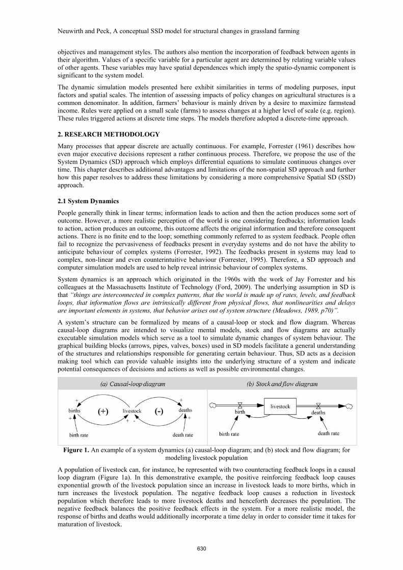
A system’s structure can be formalized by means of a causal-loop or stock and flow diagram. Whereas causal-loop diagrams are intended to visualize mental models, stock and flow diagrams are actually executable simulation models which serve as a tool to simulate dynamic changes of system behaviour. The graphical building blocks (arrows, pipes, valves, boxes) used in SD models facilitate a general understanding of the structures and relationships responsible for generating certain behaviour. Thus, SD acts as a decision making tool which can provide valuable insights into the underlying structure of a system and indicate potential consequences of decisions and actions as well as possible environmental changes.

Figure 1. An example of a system dynamics (a) causal-loop diagram; and (b) stock and flow diagram; for

modeling livestock population

A population of livestock can, for instance, be represented with two counteracting feedback loops in a causal loop diagram (Figure 1a). In this demonstrative example, the positive reinforcing feedback loop causes exponential growth of the livestock population since an increase in livestock leads to more births, which in turn increases the livestock population. The negative feedback loop causes a reduction in livestock population which therefore leads to more livestock deaths and henceforth decreases the population. The negative feedback balances the positive feedback effects in the system. For a more realistic model, the response of births and deaths would additionally incorporate a time delay in order to consider time it takes for maturation of livestock.

630


The conceptual causal loop diagram can be translated to an executable stock and flow diagram (Figure 1b). To do so, the elements belonging to a system must be transformed into stocks, flows and converters - these represent the basic building blocks of SD models. Stocks, also called state variables, represent quantities that accumulative over time which are calculated as the numerical integration of ordinary differential equations (ODEs). Stocks (livestock) are modified by material or informational flows. Flows (births and deaths) are measured over intervals in time and either augment or deplete the stock variable. These flows are a function of converters (birth rate and death rate) and in this particular case have a feedback relationship with the state variable (livestock). This graphical representation of systems also serves as an effective tool for brainstorming and participatory model design (Maxwell and Voinov, 2005).

SD is a powerful approach for simulating cross-disciplinary problems in the fields of ecology, economics, physics, resource management, politics, management, engineering or industrial operations. One of the most popular SD applications is the World3 model for the simulation of global economic and population growth introduced in the book ‘The limits to growth’ by Meadows et al., (1972). Furthermore, a variety of SD models have been applied to more specific issues such as water resource conflict management (e.g. Nandalal and Simonovic, 2003), agriculture (e.g. Johnson et al., 2008) and urban planning (e.g. Forrester, 1969).

Although SD is suitable for simulating temporal changes of a system, a common shortcoming in SD applications is the inability to capture spatial dynamics of a system. Most SD applications fail to incorporate complex spatial topologies. Therefore, a main objective of the proposed research includes addressing this methodological shortcoming by incorporating the spatial dimension. The framework introduced in the next chapter is intended to lay the foundations for a Spatial System Dynamics (SSD) approach.

2.2 Spatial System Dynamics System dynamics suffers from several limitations when it comes to incorporating space. Since many modeling topics related to environmental issues are spatially distributed problems (Fedra, 2005), the applicability of traditional SD is restricted.

As a key tool for spatial data management and analysis, a Geographic Information System (GIS) is well suited to address the limitations of a traditional SD approach. The GIS component serves three main purposes:

1. As a spatial data management tool; 2. As a spatial analysis tool; and 3. As a map-based visualization tool.

Consequently, the synthesis of SD and GIS produces added value for this application, as it could provide both the temporal and spatial modeling capabilities required to more accurately represent real-world systems.

In order to join the strengths of SD and GIS, a technical linkage can be envisioned. De Smith et al., (2007) distinguish between the following approaches for linking software:

1. Loose Coupling: The software components interact via data exchange. 2. Moderate Coupling: The link between software components is based on a shared database access. 3. Tight Coupling: A standard is used to invoke commands from both systems during the program execution

(e.g. .NET standard). 4. Embedding: The required functionality is integrated within the dominant system (SD or GIS) using the

underlying programming language.

The loose and moderate coupling approaches are more straightforwardly implemented; however, both approaches have limitations in performance and processing efficiency. Embedding the spatial model into the dominant program (GIS) has the advantage that all functions and data resources of the GIS can be used (Pelizaro and McDonald, 2006). Thus, this integration strategy can provide access to a consistent user interface and data structure.

3. PROPOSED SSD APPLICATION: CHANGES IN GRASSLAND FARM STRUCTURES

The following application presents an original SSD model for simulating grassland farm structural changes. The model can be considered a finite resources competition model; a concept inspired by a water allocation model published by Nandalal and Simonovic (2003).

The current version of model is developed using Vensim SD modeling and simulation software and is in the development phase, therefore no stock and flow diagrams or simulations have been produced at this time. However, a conceptual, qualitative SD and SSD description of a proposed two-Farm Structural Dynamics (2FaSD) model is discussed.

631


3.1 Causal System Structure The causal loop diagram for the 2FaSD model graphically presents the competition between two farms; Farm A and Farm B and each farm is represented by a subsystem; Farm Subsystem A and Farm Subsystem B, respectively (Figure 2). These farm subsystems are linked to each other through competition over limited grassland resources. Furthermore, each farm subsystem comprises an economic subsystem; referred to as

Economic Subsystem A and Economic Subsystem B. These subsystems include financial and managerial decisions such as raising credit and investments in machinery.

The desire for farmers to expand their farmland area is based on individual aspirations and opportunity costs - defined as the difference between the farmers’ income and a theoretical income which could be gained through off-farm employment. Aspirations vary among farmers based on personal values, goals, expectations and desired standards of living. As the difference between opportunity costs and aspirations increases, farmers’ level of satisfaction would be assumed to decrease. The key assumption is that a lower satisfaction with the farming business leads to a continuous grasslands retreat, whereas high satisfaction triggers land use intensification in conjunction with an increasing fight for more farmland as the land use intensity (number of animals per area) comes closer to the ecological carrying capacity.

In addition to farmer satisfaction, the expansion dynamic of a farm is also crucially affected by shadow prices. The shadow price represents theoretical profits which could be gained through the acquisition of additional farmland and is dependent on the revenue potential and operating costs associated with the additional farmland. Operating costs depends on the level of investment in machinery and transportation costs associated with the physical distance between the farmstead and a grasslands plot. Shadow prices are thus spatially dependent, spatially dynamic, and specific to each farm. Regional differences in available agricultural technologies are presently neglected.

The increasing shadow prices associated with farmland expansion and cumulative transportation costs mitigate the farmer expansion dynamic. Furthermore, a restriction for level of intensification and expansion is given by the availability of labour. This threshold varies as a function of investments in machinery, since the degree of mechanization effects the requirement for labour.

Figure 2. Causal loop diagram of grassland competition between two farms

The 2FaSD system outlined in this chapter also exhibits spatially distributed characteristics. In the next chapter, techniques to implement a SSD model for the simulation of this system are discussed.

3.2 SSD: Anticipated Implementation

The implementation of the 2FaSD model requires the incorporation of both spatial data models as well as concepts of geospatial analysis to take distributed environmental conditions and dynamically changing transportation costs, ownership structures or land use intensities into account. These capacities are provided by the software ArcGIS.

Hence, for the implementation of the 2FaSD model an embedding of the SD software Vensim in ArcGIS is planned. The Python API for ArcGIS can be used to develop a graphical user interface. This Python code may be supplemented with Vensim functions. In order to ensure compatibility, Vensim libraries are wrapped in pure Python code using the foreign function library ctypes. Alternatively, the Dynamic Link Library (DLL) function provided by Vensim could be used to export and link the SD model with ArcGIS by providing appropriate interface parameters. The main advantage of this procedure is that the system model in Vensim could still be developed using graphical stock and flow diagrams.

632


The simulation process involves mutual interaction between Vensim and ArcGIS. The interaction is initialized by the Vensim model. The proportion of grassland belonging to each farmer and the farming intensity change based on different economic, physical, and individual characteristics and preferences according to the causal assumptions in the SD model. This change triggers the conversion of numerical values to spatial representation in ArcGIS, which is evaluated by means of geospatial algorithms. Subsequently, the output of the spatial analysis serves as an input parameter for the recalculation of state variables for each farm system in Vensim, which are in turn converted and analyzed in ArcGIS. In order to minimize errors due to asynchronous interactions, the execution of the Vensim simulation may be interrupted during the recalculation of spatial variables (e.g. transportation costs). Moreover, the update frequency in ArcGIS could be adjusted to match the temporal resolution of the Vensim simulation.

One major challenge of interfacing the SD software Vensim with the spatial modeling software ArcGIS results from the differences in the structure of the output data. For instance, the grassland allocated to a farm is represented by means of a state variable in Vensim. The changes in this variable have to be transferred to a discretized spatial representation such as raster arrays before they are able to be used in ArcGIS. The conversion from a numeric value to a raster data model may be based on the principle of ‘successive least value grassland reduction’. This means that the grassland with the least respective value to the previous owner is successively allocated to the expanding farm (grassland value is spatially dependent and specific to each farm). The expected output of this procedure is a time-series of raster maps showing the evolution of farm structure over time, similar in concept to the physical farm size change depicted in Figure 3.

Besides the succession of spatial ownership transformation, logic has to be developed to convert between numeric areas (Vensim) and spatial areas represented by the raster array (ArcGIS). One way to avoid conversion errors is to assign proportional ownership rates to raster cells, i. e. one raster cell can be shared by multiple farms. However, since ordinary GIS data formats do not permit the assignment of multiple values to a single raster cell, the incorporation of 3D numpy (Python module) arrays is envisaged.

4. CONCLUSIONS AND FUTURE DEVELOPMENT

A framework for spatial-temporal modeling is required for a more realistic approach to modeling changes in grassland farm structural change. To achieve this, we propose a SD and GIS coupling approach for modeling and simulation of spatial system dynamics (SSD).

A continuous SSD Farm Structure Dynamics (2FaSD) simulation model is proposed to capture the spatial and temporal dynamics of grassland farm structural changes. Currently, the model is in its infancy stage and the next task in development includes transferring the 2FaSD model from current causal-loop form into a numerical stock and flow simulation model. The expected outcome of model simulation includes a time series of maps which incorporates economic, physical, social, and managerial contributions to changes in grassland farm structure. Ultimately, the purpose of engaging in the modeling and simulation process is to learn about the system and its behaviour to aid the decision making process.

Figure 3. Conceptual diagram of farm expansion in time and space; schematic of anticipated 2FaSD model output

633


Effective SD model building requires a good understanding of the system; in this instance the grasslands farming system. Since the present version of the SD grasslands farming model has been developed by the authors, it would be beneficial to engage agrarian economists and practicing grassland farmers to achieve a more realistic and credible representation of 2FaSD model structure. As such, the systems model development process is in itself, dynamic and additional 2FaSD elements may be added in the future. Although the current application is based on competition between 2 farms, it is foreseeable that the 2FaSD model and methodology may be extended to consider more than two farms in the future.

ACKNOWLEDGMENTS

We appreciate the financial support provided by the Austrian Science Fund (FWF) through the Doctoral College GIScience (DK W 1237-N23) to the first author and the Natural Sciences and Engineering Research Council (NSERC) of Canada CGS doctoral scholarship to the second author.

REFERENCES

Balmann, A. (1997). Farm-based modelling of regional structural change: A cellular automata approach. European review of agricultural economics, 24(1), 85-108.

Bossel, H. (2007). Systems and models: complexity, dynamics, evolution, sustainability: BoD-Books on Demand.

Dabbert, S., and J. Braun (2006). Landwirtschaftliche Betriebslehre: Grundwissen Bachelor;[mit] 52 Tabellen: Ulmer.

De Smith, M.J., M.F. Goodchild, and P.A. Longley (2007). Geospatial analysis: a comprehensive guide to principles, techniques and software tools: Troubador Publishing Ltd.

Fedra, K. (2005). Beyond GIS: integrating dynamic simulation models and GIS for natural resources and environmental management. Map Middle East, 2006 Proceedings.

Ford, A. (2009). Modeling the environment: Island Press. Forrester, J.W. (1961). Industrial dynamics (Vol. 2): MIT press Cambridge, MA. Forrester, J.W. (1969). Urban dynamics. Forrester, J.W. (1992). Policies, decisions and information sources for modeling. European Journal of

Operational Research, 59(1), 42-63. Forrester, J.W. (1995). Counterintuitive behavior of social systems. collected papers of Jay W. Forrester. Freeman, T., J. Nolan, and R. Schoney (2009). An Agent-Based Simulation Model of Structural Change in

Canadian Prairie Agriculture, 1960–2000. Canadian Journal of Agricultural Economics/Revue canadienne d'agroeconomie, 57(4), 537-554.

Happe, K., K. Kellermann, and A. Balmann (2006). Agent-based analysis of agricultural policies: an illustration of the agricultural policy simulator AgriPoliS, its adaptation and behavior. Ecology and Society, 11(1), 49.

Johnson, T., J. Bryden, K. Refsgaard, and S. Lizárraga (2008). A system dynamics model of agriculture and rural development: the TOPMARD core model. Communication présentée au 107e Séminaire de l’EAAE “Modelling of Agricultural and Rural Development Policies”, Séville, 29.

Kellermann, K., K. Happe, C. Sahrbacher, A. Balmann, M. Brady, H. Schnicke, and A. Osuch (2008). AgriPoliS 2.1–Model documentation. Halle, Germany, IAMO.

Maxwell, T., and A. Voinov (2005). Dynamic, Geospatial Landscape Modeling and Simulation. In D. J. Maguire, M. Batty & M. F. Goodchild (Eds.), GIS, Spatial Analysis and Modeling. Redlands: ESRI.

Meadows, D.H. (1989). System dynamics meets the press. System Dynamics Review, 5(1), 69-80. Meadows, D.L., D.H. Meadows, J. Randers, and W.W. Behrens III (1972). The Limits to Growth: A Report

to The Club of Rome (1972): Universe Books, New York. Nandalal, K.D.W., and S.P. Simonovic (2003). Resolving conflicts in water sharing: A systemic approach.

Water Resources Research, 39(12). Pelizaro, C., and D. McDonald (2006). Spatial (GIS-based) decision support system for the Westernport

region. Zimmermann, A., T. Heckelei, and I.P. Dominguez (2006). Working paper: Literature Review of Approaches

to Estimate Structural Change: SEAMLESS: System for Environmental and Agricultural Modelling, Linking European Science and Society.

634

a conceptual spatial system dynamics (ssd) model for ...mssanz.org.au/modsim2013/b2/neuwirth.pdf ·...

Documents