a computational optimization of magnetic system consists

Republic of Iraq Ministry of Higher Education and Scientific Research AL-Nahrain University College of Science

A Computational Optimization of Magnetic System Consists of

Deflector and Lens

A Thesis Submitted to the College of Science of Al-Nahrain

University in Partial Fulfillment of the Requirements for the Degree of Master of Science in Physics

By

Ahmad Hussein Ali (B.Sc.2006)

Supervised by

Dr. Ahmad Kamal Ahmad & Dr. Oday Ali Hussein

In

Thou Al-Hujaa 1429 A. H. December 2008 A. D.

حيم ب حمن الر الر سم الله

)39(يس للإنسان إلا ما سعى أن ل و م يجزاه ث )40(سعيه سوف يرى أن و

)41(الجزاء الأوفى صدق الله العظيم

النجم سورةمن

Certification I certify that this thesis entitled “A Computational

Optimization of Magnetic System Consists of Deflector and

Lens” is prepared by Mr. Ahmad Hussein Ali under our

supervision at the College of Science of Al-Nahrain University in

partial fulfillment of the requirements for the degree of Master of

Science in Physics.

Supervisor: Dr. Ahmad K. Ahmad Supervisor: Dr. Oday A. Hussein

Title: Assistant Professor Title: Lecturer

Date: / /2008 Date: / /2008

In view of the recommendations, I present this thesis for debate by

the examination committee.

Dr. Ahmad K. Ahmad

Title: Assistant Professor

Head of Physics Department

Date: / /2008

Dedicated to

My Family

Acknowledgments First of all, I would like to thank almighty ALLAH for gifting me a

spot light, which has given me hope, patience, and a new thinking for a

better life.

Secondly, I would like to thank the messenger of peace Mohammed, the

prophet of humans.

I would like to express my sincere thanks and deep appreciation to my

supervisors, Dr. Ahmad K. Ahmad and Dr. Oday A. Hussein for suggesting

the project of research, helpful discussions and comments throughout this

work, and for reading the manuscript of this thesis.

A special thank to Mr. Mahdi Ahmad for valuable assistance during

the work.

I am grateful to the Dean of College of science and the staff of the

Department of physics at Al-Nahrain University for their valuable support

and cooperation. I thank the staff of the library of Al-Nahrain University.

My special thanks to all my friends for encouragement and support during

the work.

Last but not least, I would like to record my deep affection and thanks

to my parent for their moral support and patience throughout this work.

Ahmad

Contents

Abstract.................................................................................................. I

List of Symbols........................................................................................ III

Chapter One

Introduction

1.1 Introduction...................................................................................... 1

1.2 Magnetic Deflector........................................................................... 1

1.3 Types of Magnetic Deflector............................................................ 1

1.4 Magnetic Lenses............................................................................... 2

1.5 Type of Magnetic Lenses.................................................................. 3

1.6 Properties of Magnetic Lenses......................................................... 3

1.7 Advantage of Magnetic Lenses and Deflectors................................ 4

1.8 Historical Review............................................................................. 4

1.9 Optimization Method........................................................................ 7

1.14 Aim of the theses........................................................................... 8

Chapter Two

Theoretical Considerations

2.1 Introduction......................................................................................

9

2.2 Paraxial-Ray Equation in Magnetic Fields...................................... 9

2.3 Optical Parameters and Initial Condition........................................ 10

2.4 Magnetic Deflection Fields............................................................ 12

2.5Magnetic Scalar Potential Calculation........................................... 13

2.6 Pole Piece Reconsideration............................................................ 15

2.7 The Moving Objective Lens (MOL) Concept.................................. 15

2.8 Aberrations of Axially Symmetric Electron-Optical Systems...........

17

2.8.1 Spherical aberration................................................................. 17

2.8.2 Chromatic aberration............................................................... 19

2.8.3 Radial and spiral distortions................................................... 21

Chapter Three

Results and Discussion

3.1 The Behavior of the Magnetic Deflector and Lens at Difference

Values of Length and Angle of Coil...................................................

25

3.2 Design Using Exponential Model......................................... 26

3.3 Electron Beam Trajectory................................................................ 30

3.4 Infinite Magnification Condition...................................................... 33

3.4.1 Effects of changing the length.................................................. 33

a- Relative spherical and chromatic aberration coefficients…..... 33

b- Relative radial and spiral distortion coefficients...................... 37

3.4.2 Effects of changing the angle................................................... 40

a- Relative spherical and chromatic aberration coefficient.......... 40


3.5 Zero Magnification Condition.......................................................... 47

3.5.1 Effects of changing the length.................................................. 47

a- Relative spherical and chromatic aberration coefficients........ 47

b- Relative radial and spiral distortion coefficients..................... 50

3.5.2 Effects of changing the angle.................................................... 52

a- Relative spherical and chromatic aberration coefficients........ 52


3.6 Pole Pieces Reconstruction............................................................. 59

Chapter Four

Conclusions and Suggestions for Future Work

4.1 Conclusions...................................................................................... 60

4.2 Recommendations for Future Work.................................................. 61

Reference........................................................................................... 62

Abstract

A computation investigation on the design of magnetic deflection and

focusing system using the synthesis approach of optimization method has

been done. By solving the paraxial ray equation using the Range-Kutta-

Nystrom method the trajectories of the electron beam and the optical

properties of the magnetic deflection and focusing system under infinite and

zero magnification conditions has been computed.

The synthesis approach of optimization method is used in the present

work to finding the optimum design of magnetic deflection and focusing

system which give rise to the minimum spherical, chromatic, spiral

distortion, and radial distortion aberration.

The toroidal deflection coil is used as the source of magnetic field, and

then the field distribution is determined by using an exponential function.

The moving objective lens concept is included in the computation of system

field.

The system aberration has been minimized by changing the geometrical

shape of the toroidal coil, where the length and angle of the coil varied. By

using the optimum axial field distribution, the pole pieces shape which gives

rise to these field distributions is found by using the reconstruction method.

Computation shows that the smaller aberration coefficients occur when

the length of the coil (H= 23mm) and angle of the coil (Ø=61o). The

relationship between the four coefficients and length and angle of the coil is

inverse proportional in the cases of zero and infinite magnification

conditions, therefore, provides us with the possibility of operating the

system with high efficiently in different operation conditions of the system.

List of Symbols a The field width at half maximum Bm / 2.

B(z) Magnetic flux density (Tesla).

Bm Maximum value of axial magnetic flux density distribution (Tesla).

Bx(z) The deflection field at the axis of an air core toroidal yoke (Tesla).

Cc Chromatic aberration coefficient (m).

Cs Spherical aberration coefficient (m).

D Distortion coefficient (m).

D(z) Deflection magnetic flux density (Tesla).

Drad Radial distortion coefficient (m).

Dsp Spiral distortion coefficient (m).

d Displacement by the first magnetic deflector (m).

Eo Energy of electron beam.

e Electron charge (1.6 ×10-19 C).

Fp Projector focal length (mm).

H The length of the toroidal coil (mm).

h Solution of paraxial ray equation.

L The length of the system field.

M Liner magnification.

m Electron mass (m = 9.1 × 10-31 Kg).

NI Magnetic excitation (Ampere-turns).

NI/ (Vr)0.5 Magnetic excitation parameter (Ampere-turns/(Volt)0.5).

R Radial displacement of the beam from the optical axis (m).

Rp(z) Radial height of the pole pieces along the optical axis (m).

r Distance of the corresponding object point from the axis (m).

rs Fluctuation in the electron beam focus.

Va Accelerating voltage (Volt).

Vp Pole piece potential (Volt).

Vr Relativistic corrected accelerating voltage (Volt).

Vz=V(z) Axial magnetic scalar potential (Volt).

X and Y Two independent solutions of the paraxial-ray equation.

z Length of the optical axis along the system (m).

zi Image plane position (m).

zo Object plane position (m).

α Trajectory angle with system axis (degree).

β Angle of the arriving electrons (degree).

ΔEo Fluctuation in the electron beam energy.

μo Permeability of free space (μο= 4 π*10-7 H.m-1).

ϕ Angle of the coil (degree).

CChhaapptteerr OOnnee

Introduction

Chapter One

Introduction 1.1 Introduction

In many electron beam instruments, such as scanning electron

microscopes and scanning electron beam lithography systems are usually use

a magnetic lens to focus a(charge) particle beam , and magnetic deflection

coils mounted with in the lens.

In particular, the relationship between focusing magnetic field of the

lens and the deflection field must be optimized for minimum aberration and

normal landing angle [Lencova and Wisselink 2001].

1.2 Magnetic Deflectors The magnetic deflectors are used to steer the beam in the desired

direction [Philip Coane 1999].

The most common and classical type of deflection is used in cathode ray

tubes and scanning electron microscopes . Its purpose is to scan the beam

over a surface [Szilagyi 1988].

1.3 Types of Magnetic Deflector In the magnetic deflectors, two geometries are common

a- Toroidal magnetic deflection system: Systems of this kind are used in

television tubes, and in scanning microscopes for deflecting the electron

beam. In toroidal structure figure (1-1).Two pairs of coils, rotated at 90 ◌

Figure (1-1) Toroidal deflection coil [Hawkes and Kasper 1989].

b- Saddle coil: saddle coil, shown in figure (1-2) is usually enclosed in a

ferrite sheathe, there by reducing the wastage of flux. The shielding is

omitted only in devices designed to function at high deflection

frequencies in order to decrease the inductance[Hawkes 1989].

Figure (1-2) Saddle deflection coil (Hawkes and Kasper 1989).

1.4 Magnetic Lenses To focus an electron beam, a magnetic lens employs the magnetic field

produced by a coil carrying a direct current [Egerton 2007].Manufacturing

of magnetic lenses is usually more complicated than that of electrostatic

lenses.

The magnetic lenses have extensive applications in such areas as

electron microscopy and cathode ray tubes [Humphries 1999].

1.5 Types of Magnetic Lenses

Magnetic lenses can be classified from various points of view. For

example, one can mention (a) thick or thin lenses, according to the change in

the slope of the trajectory of the beam passing through the lens, (b) strong or

weak lenses depending on whether their focal points are situated inside or

outside the magnetic field, (c) symmetric or asymmetric lenses depending

upon whether there exists a middle plane perpendicular to the lens axis about

which the geometrical arrangement of the lens is symmetric or not, (d)

doublet or singlet depending on whether the lens has two or one air gap.

Furthermore, magnetic lenses may be long or short, iron-free or shrouded by

ferromagnetic materials.

Magnetic lenses may be classified according to the number of pole

pieces in the lens. According to the criteria magnetic lenses can be classified

into four types namely, single pole piece, double pole piece, triple pole

piece, and the iron-free [Szilagyi 1988].

1.6 Properties of Magnetic Lenses The lens properties can be determined once the real lens field is

replaced by an ideal rectangular field of length L. Physically this ideal field

is that of a solenoid of length S and diameter 2/3D carrying the same ampere

– turns NI ( excitation) (i.e. number of turns × D.C. current). The diagonal

L of the solenoid is related to the real lens geometry by [Lencova 1997]:

2 3⁄ (1-1)

The maximum magnetic flux density Bmax is given by [Lencova and

Wisselink 2001]:

1‐2 ⁄

where L is geometrical parameter, µo is the permeability of free space.

Therefore, the magnetic field generated by a magnetic lens depends on its

shape and excitation NI.

The distinctive feature of magnetic lenses is that their optical properties

are dependent on the charge to mass ratio of the particles. In magnetic lenses

the particle trajectories depend on the particles mass, where heavy particles

are less focused than light ones.

Magnetic lenses are used for forming electron optical system which

transforms an 'object' into 'image' [Goodhew et al 2001].

1.7 Advantage of Magnetic Lenses and Deflectors Compared with electrostatic lens and deflector, magnetic lens and

deflector have some advantages [Liu 2005]:

1- High stability

2- Low aberration

3- High sensitivity

1.8 Historical Review Many researchers attempted to design and optimization of combined

magnetic deflector and lens systems with minimum aberrations, for

examples:

[Munro (1974)] derived the formula for calculating the first-order

optical properties, third-order aberrations coefficient, and first-order

chromatic aberrations for magnetic combined deflective focusing system.

His formulae are applicable to the general case in which the lens and

deflector field are superimposed on one another.

[Munro (1975)] introduced the methods for computing the optical

properties of any combination of magnetic lenses and deflection yokes,

including the most general case in which the lens and deflector fields may

physically be superimposed.

[Ohiwa (1977)] presented the considerations and results of designing air-

core scanning systems comprising round lenses and saddle type deflection

coils.

[Kuroda (1980)] introduced the method for calculating the deflective

aberration for deflection system with two deflectors and a lens by using the

independent aberration of each deflector. The method gives the deflective

aberrations without the calculation of deflection fields or paraxial

trajectories when the conditions (rotation angle and coil current) of each

deflector are changed.

The numerical analysis of magnetic deflector in electron beam

lithography system was carried out by [Munro and Chu (1981b)].

Formulae were derived for calculating the first and third harmonic

components of the magnetic deflection field, for both toroidal and saddle

yokes, either in free- space region by using the Biot- Saverd law on in

presence of rotationally symmetric ferromagnetic materials by using the

finite element method.

A combined system consisting of round lenses and magnetic deflector

with superimposed fields had been studied by [Jiye (1981)]. The general

expressions for superimposed fields and trajectories were obtained. The

Gaussian optical properties of the system were discussed and the effect of

magnetic deflector on the round magnetic and electrostatic lens might be

considered as the linear transformations for Gaussian trajectory parameters.

Then the expressions for calculating the aberrations were given in a compact

matrix form appropriate for numerical computation.

A focusing and deflection system with vertical landing and reduced

aberrations was developed by [Kuroda et al(1983)], for direct electron-

beam lithography. The system consisted of two magnetic lenses and a

magnetic deflector. The excitations of the lenses were opposite to each other.

The deflector, which had saddle coils, was set inside the first lens.

[Lencova (1988)] summarized some basic ideas used in the design of

combined deflection and focusing system.

The fifth order aberration coefficient formulas for deflective focusing

systems have been derived by several authors; [Yu Li et al (1993)];[ Uno Y

(1995)]; and [ Kangyan and Tang (1999)].

[Wang et al (2000)] developed differential algebraic method (DA),

which implement the DA method to arbitrary high order in visual C++, and

applied it to the analysis of electron lenses and deflection systems

separately.

[Wang (2002)] introduced a new mathematical method, differential

algebraic (DA) method, into the aberration of combined focusing-deflection

system. This method is first introduced by Berz (1989) into accelerator

physics and achieved great success.

[Teruo Hosokawa (2002)] derived the relationships between the third-

and fifth-order complex aberration coefficients in electron optical deflective

focusing system.

[Alamir (2003)] computed the spiral distortion of magnetic lenses with

field distribution in the form of an inverse power law.

[Alamir (2004)] computed the chromatic aberration of magnetic lenses

with a field distribution in the form of an inverse power law.

[Alamir (2005)] calculated the optical properties of monopole, multipole

magnetic lenses.

[Yan Ren et al (2007)] studied the aberration theory of combined

electron focusing-deflection system with a rotating deflection field following

the rotation of the electron.

1.9 Optimization Methods The desire to produce electron and ion optical systems with prescribed

optical properties and as small aberrations as possible is as old as electron

and ion optics itself [Szilagyi 1988].

Optimization is the search for such electron and ion optical element that

would provide the required optical properties with minimum aberrations.

There are two different approaches to optimization: analysis and synthesis.

The method of analysis is based on trail and error. The designer starts

with certain set of given elements (electrodes or pole pieces) and tries to

improve their performance by analyzing the optical properties and varying

the geometrical dimensions as well as the electric or magnetic parameters of

the system until a satisfactory performance is achieved.

Owing to the infinite number of possible configurations this procedure is

extremely slow and tedious. It can yield quick and reliable results only if a

reasonable guess of the design is already available before the work

starts[Szilagyi 1988].

Optimization by synthesis has always been one of the most ambitious

goals of electron and ion optics. This approach is based on the fact that any

imaging field, its optical properties and aberrations are always totally

determined by axial field distribution.

1.10 Aim of the Thesis The aim of this work is to find the optimum design of magnetic system

which consists of magnetic deflector and lens which gives rise to the

minimum spherical, chromatic, spiral distortion and radial distortion

aberration. The synthesis approach of optimization method is used in the

present work.

In the calculations; the toroidal deflection coil is used as the source of

magnetic field, then the exponential field distribution model is used. Also,

the moving objective lens concept is included in the computation of

deflection field.

Deflection aberrations can be minimized for the exponential field

distribution model by changing the shape of the deflection coil, where the

length and angle can be varied. By using the optimum axial field

distribution, the pole pieces design which gives rise to this field distribution

can be found by using reconstruction method.

CChhaapptteerr TTwwoo

Theoretical

Considerations

Chapter Two

Theoretical Considerations

2.1 Introduction A charge particle beam is a group of particles that have about the

same kinetic energy and move in about the same direction

[Humphries 2002]. The high kinetic energy and directionality of

charged particles in beams make them useful for applications.

Charged particle beams have continually expanding applications in

many branches of research and technology. Recent active areas include

flat-screen cathode-ray tubes, and beam lithography for microcircuits.

2.2 Paraxial-Ray Equation in Magnetic Fields The paraxial ray equation in axially symmetric magnetic fields can

be written as [Tsimring 2007]:

8 0

1 0.978 10

(2-1)

where e and m are the charge and mass of electron respectively, and Vr

is the relativistially corrected accelerating voltage which is given

by ilagyi 1988].: [Sz

(2-2)

where Va is the accelerating voltage.

Equation (2-1) is a second order differential equation. This equation

was solved numerically using Range-Kutta-Nystrom method

[Kreyszig 1983]. In present work we check our results to solve the

equation (2-1) analytically by the method of undetermined coefficients

using MATLAB program [Karris 2004].

2.3 Optical Parameters and Initial Conditions

Some definitions of the optical parameters used in the present work

are given in this section.

Object side: The side of optical design at which the charged particles

enter.

Image side: The side of optical design at which the charged particles

leave.

The object plane ( ): The plane at which the physical object is placed,

or a real image is formed from a previous optical design, on the object

side.

OZ

The image plane ( ): The plane at which the real image of the object

plane is formed, on the image side.

iZ

OZ

Focal length (F): The focal length is the distance between the principle

plane and the foucs [Tsimring 2007].

Magnification ( M ): In any optical system the ratio between the

transverse dimension of the final image and the corresponding

dimension of the original object is called the lateral magnification˝M˝:

(2-3)

There are three magnification conditions under which an optical

design such as lens or deflector can operate, namely [Munro 1975]:

(i) zero magnification condition: In this operational condition ∞−=OZ

as shown in figure (2-1). As an example, the final probe-forming lens

in a scanning electron microscope (SEM) is usually operated under this

condition.

Figure (2-1): Zero magnification condition.

(ii) Infinite magnification condition: In this case ∞+=iZ as shown in

figure (2-2). As an example, the objective lens in a transmission

electron microscope ( TEM ) is usually operated under this condition.

Figure (2-2): Infinite magnification condition.

(iii) Finite magnification condition: Under this operational condition

and are at finite distances, as shown in figure (2-3). As an example

the electrostatic lens in field-emission gun is usually operated under

this condition.

OZ

iZ

Figure (2-3): Finite magnification condition.

2.4 Magnetic Deflection Fields

In magnetic deflector, two geometries are common: saddle and toroidal

coils. In the present work, the toroidal coil is taken as the source of magnetic

field.

The method used for calculating the deflection yoke fields depends on

whether the deflection coils are near the magnetic materials or not [Septier

1980]. If the deflection yoke is in a free-space region, its field can be

calculated using the Biot-savart's formula. The deflection field at the axis of

an air-cored toroidal coil, Bx(z), is obtained using the formula given by

[Munro 1975]:

sin Ø √ √ √ √ (2-4)

where NI is the magnetic excitation, Ø is the angle of the toroidal coil, R

and r are the outer and inner radius of the toroidal coil, respectively, Bx(z) is

deflection field of toroidal yoke and h and l are defined in figure (1-1).

If the deflection coil is near magnetic materials, the Biot-savart's formula

is no longer applicable. Instead, some numerical technique must be used,

such as the finite-element method. This method can be used for either

toroidal or saddle yokes, wound on magnetic formers or placed inside

magnetic circuits.

2.5 Magnetic Scalar Potential Calculation The magnetic scalar potential is an essential factor for finding the pole

piece shape. Thus, it is important to determine the magnetic scalar potential

distribution along the lens and deflector system length At the lens axis the

axial flux density distribution is given by. [Al-Obaidi1995].

(2-5) where Bz is the axial flux density distribution , Vz is the axial potential

distribution, and µo is the permeability of free space. The magnetic scalar

potential Vz can be calculated by integrating equation (2-5) along the lens

and deflector system axis.

(2-6)

i.e.,

′ 0.5 "" "

(2-7)

where a and b are the axial magnetic field limits.

It is intended to find the magnetic scalar potential along the lens and

deflector system as a tabulated data set. Thus the lens and deflector system

axis (i.e. the interval where the axial magnetic field exists) is divided into (n-

1) subintervals where n is the number of points (z , Bz). The axial magnetic

flux density Bz can be approximated by the well-known cubic spline for each

subinterval as follows:

′

(2-8)

where zi ≤ z ≤ zi+1, and i =1, 2, 3, …. , (n-1). Equation (2-6) can be

executed over each subinterval with the aid of equation (2-8); the result is

the following recurrence formula,

" ′′ (2-9) where hi = ( zi+1 – zi ) is the width of each subinterval. Equation (2-9) can be

written in the following simplified form

(2-10)

Where

′2

"2

′′3 2

0.5

0.5

2 "

Since the axial magnetic flux density considered in this work is symmetrical,

one can put

The recurrence formula (2-10) can thus be written in the following form,

(2-11 )

for each subinterval zi ≤ z ≤ zi+1. Therefore, one can get the magnetic scalar

potential V (z) along the lens and deflector system interval zi ≤ z ≤ zn . The

above algorithm has been formulated into a MATLAB 2008.

2.6 Pole Piece Reconsideration The pole piece shape can be design by using the following equation,

⁄

(2-12)

where Rp is the radial height of the pole piece and Vp is the value of the

potential of the pole piece. This equation used by [Szilagyi 1984] to reconstruct the pole piece shape

of magnetic deflector and lens.

2.7 The Moving Objective Lens (MOL) Concept The concept of moving objective lens (MOL) was introduced first by

[Ohiwa et al 1971]. Ohiwa pointed out that the aberrations of a combined

focusing and deflection system can be greatly reduced by using an

arrangement of the type shown in figure (2-4).

A point source of electrons, emitted from zo, is imaged by a lens at zi. The

beam is deflected by the first deflector so that it enters the lens off axis, a

second deflector, placed inside the lens. This so- called "moving objective

lens" (MOL) reduces the effect of the off axis lens aberrations. The spherical

and chromatic aberration of the lens can be kept small by having a short

working distance L2 (see figure 2-4). At the same time the deflection

aberrations can be kept small by having a large distance L1 from the first

deflector to the image plane [Marton 1980]. This concept has been analyzed

theoretically by [ Ohiwa et al. 1971] and [Goto and Soma 1977], and has

been used in practical designs by [Munro 1975] , [Ohiwa 1978], and [Goto

et al. 1978].

Figure (2-4) The moving objective lens concepts [Ohiwa 1978].

Let B(z)the axial flux density distribution for lens and D(z) the

deflection flux density required at the axis. Then, the following relation

holds [ Ohiwa 1978 and Lencova 1987].

′ (2- 13)

where d is the displacement by the first deflector (pre deflection). 2.8 Aberrations of Axially Symmetric Electron Optical

Systems

The theory of aberrations is the most extensively studied area in both

light optics and electron optics. Intensive investigations of aberrations

in axially symmetric electron-optical systems were carried out since the

1930 in connection with studies of the electron transmission microscope

problem. Their implementation provides the creation of an ideal lens that

forms stigmatic and similar images. Let us recall these assumptions: (1)

rigorous axial symmetry; (2) paraxial trajectory approximation; (3) energy

homogeneity, including the absence of time-dependent processes; and (4)

negligible space-charge fields and small effects of electron diffraction.

Violation of at least one of these conditions leads to aberrations that are

responsible for blurred or distorted images and complicate beam transport

problems [Tsimring 2007]. 2.8.1 Spherical Aberration

The spherical aberration is one of the most important geometrical

aberrations; result from violation of paraxial trajectory approximation.

The problem of spherical aberration is fundamental in electron

microscopy, in which objects are very small and arranged close to the optical

axis [Tsimring 2007].

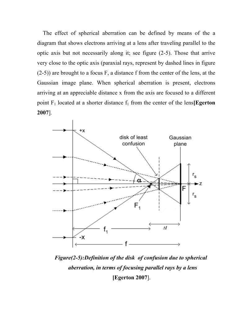
The effect of spherical aberration can be defined by means of the a

diagram that shows electrons arriving at a lens after traveling parallel to the

optic axis but not necessarily along it; see figure (2-5). Those that arrive

very close to the optic axis (paraxial rays, represent by dashed lines in figure

(2-5)) are brought to a focus F, a distance f from the center of the lens, at the

Gaussian image plane. When spherical aberration is present, electrons

arriving at an appreciable distance x from the axis are focused to a different

point F1 located at a shorter distance f1 from the center of the lens[Egerton

2007].

Figure(2-5):Definition of the disk of confusion due to spherical

aberration, in terms of focusing parallel rays by a lens

[Egerton 2007].

When these non-paraxial electrons arrive at the Gaussian image

plane, they will be displaced radically from the optic axis by an

amount rs given by[Egerton 2007].:

(2-14)

where Cs is the spherical aberration coefficient .

Figure (2-5) illustrates a limited number of off-axis electron

trajectories, the formation of an aberration circle, with electrons

arriving at the lens with all radial displacements (between zero and

some value x) within the x-z plane, within the y-x plane (perpendicular

to the diagram), and within all intermediate planes that contain the

optic axis. Due to the axial symmetry, all these electrons arrive at the

Gaussian image plane within the disk of confusion (radius rs) [Egerton

2007].

The spherical aberration coefficient sC of an axially symmetric

agnetic optical element is given by [Tahir 1985]: m

128⁄ 3 ⁄ 8 ′

8 ′⁄ (2-15) where r is the solution of the paraxial-ray equation with an initial

whole interval from object plane zo to image plane zi.

condition depending on the operation mode. The integration covers the

2.8.2 Chromatic aberration In light optics, chromatic aberration occurs when there is

spread in the wavelength of the light passing throu

gh a lens,

ractive index with wavelength

1

ave a thermal spread (≈ k T, where T is the temperature

drift (slow variation) and ripple (alternating

o a statistical process: not all electrons lose

the lens) that is focused to a point Q in the image plane (distance

coupled with a variation of the ref

(dispersion). In the case of an electron, the de Broglie wavelength

depends on the particle momentum, and therefore on its kinetic

energy Eo, So if electrons are present with different kinetic

energies, they will be a chromatic disk of confusion rather than a

point focus. The spread in kinetic energy can arise from several

causes.

- Different kinetic energies of the electrons emitted from the

source. For example, electrons emitted by a heated-filament

source h

of the emitting surface) due to the statistics of the electron-

emission process.

2- Fluctuation in the potential Vo applied to accelerated electrons.

Although high-voltage supplies are stabilized as well as possible,

there is still some

component) in the accelerating voltage, and therefore in the

kinetic energy e Vo.

3- Energy loss due to inelastic scattering in the specimen, a process

in which energy is transferred from an electron to the specimen.

This scattering is als

the same amount of energy, resulting in an energy spread within

the transmitted beam.

Consider an axial point source P of electrons (distance u from

v from the lens) for electrons of energy Eo as shown in figure (2-

6).

Figure(2-6):Ray diagram illustrating the change in focus and

the disk confusion resulting from chromatic aberration. With

tow object points, the image disks overlap [Egerton 2007] .

Electron of energy Eo - ∆Eo will have in image distance v - ∆v and

a f the

an

)

∆ ⁄

aberration coefficient Cc of an axially symmetric

magnetic optical element is given by [Tahir 1985]:

(2-18)

rrive at the image plane a radial distance ri from the optic axis. I

gle β of the arriving electrons is small[Egerton 2007].

∆ tan ∆ (2-16

The loss of spatial resolution due to chromatic aberration is therefore

[Egerton 2007].

(2-17)

where Cc is the chromatic aberration coefficient [Egerton 2007].

The chromatic

8⁄

The integration covers the whole interval from object plane zo to

image plane zi.

8.3 Radial and spiral distortions

n factor with position in the object or image there

are: two types of radial distortion Pincushion distortion and barrel

). Many electron lenses cause a rotation of the image,

Figure(2-7):(a) Square mesh (dashed lines ) ima

2. The presence of image distortion is equivalent to a variation of

the magnificatio

distortion.

The pincushion distortion corresponding to M increasing with

radial distance away from optical axis as in figure (2-6a), barrel

distortion corresponds to M decreasing away from the axis as in

figure (2-7b

and if this rotation increases with distance from the axis, the result

is spiral distortion figure (2-7c) and (2-8) [Egerton 2007].

ge

with pincushion distortion (solid curves); magnification M is

higher at point Q than that at point p. (b) Image showing

barrel distortion, with M at Q lower than at P. (c) Image of a

square, showing spiral distortion; the counterclockwise rotation

is higher at Q than at P [Egerton 2007].

Figure(2-8): A triangle imaged by an ideal lens, with

magnification and invertion. Image point A, B, and C are

equivelent to the object points a, b, and c, respectively

[Egerton 2007].

In from

the he

corre age

magnification M is a constant. Distortion changes this ideal

efficient (Dsp for spiral distortion and

ortion ).

an undistorted image, the distance R of an image point

optic axis is given by R=M r , where r is the distance of t

sponding object point from the axis , and the im

relation to[Egerton 2007]:

where D is distortion co

(2-19)

Drad for radial dist

If D > 0, each image point is displaced outwards, particularly

image suffers

ward relative to the ideal image and

tains straight-line

those further from the optical axis , and the entire

from pincushion distortion figure as in (2-7a). If D < 0, each

image point is displaced in

barrel distortion is present as in figure (2-7b).

For most purposes, distortion is a less serious lens defect than

aberration (spherical and chromatic aberrations), because it does

not result in a loss of image detail. In fact, it may not be

noticeable unless the microscope specimen con

feature [Egerton 2007].

The spiral and radial distortion coefficient of an axially symmetric

magnetic optical element is given by [Tsuno 1981]:

116

.2 ⁄ 3

8

′

∞

∞

(2-21)

where, x and y are two independent solutions of the paraxial-ray

equation with an initial condition depending on the operation

(2-20)

mode, the primes denote derivatives with respect to z and fp is the

projector focal length .

CChhaapptteerr TThhrreeee

Results & Discussion

Chapter Three Results and Discussion

3.1 The Behavior of the Magnetic Deflector and Lens at

m (deflector and

ging the geometrical

Different Values of Length and Angle of Coil In the present work, the properties of a magnetic syste

lens) have been studied. The toroidal yoke coil is used as the source of the

magnetic field. The optimum design is found by chan

shape of the coil via changing the values of length and angle of the coil to

give minimum values of relative spherical, chromatic, spiral distortion and

radial distortion aberration coefficients. The exponential function is given by

[Hawks1982] used for the shape of magnetic field distribution. The

procedure of the calculations is divided into four steps: The first; calculating

the magnetic field of the system, second: calculating the trajectory of the

electron beam, third calculating the relative spherical, chromatic, spiral

distortion and radial distortion aberration coefficients, and forth design the

pole piece shape .

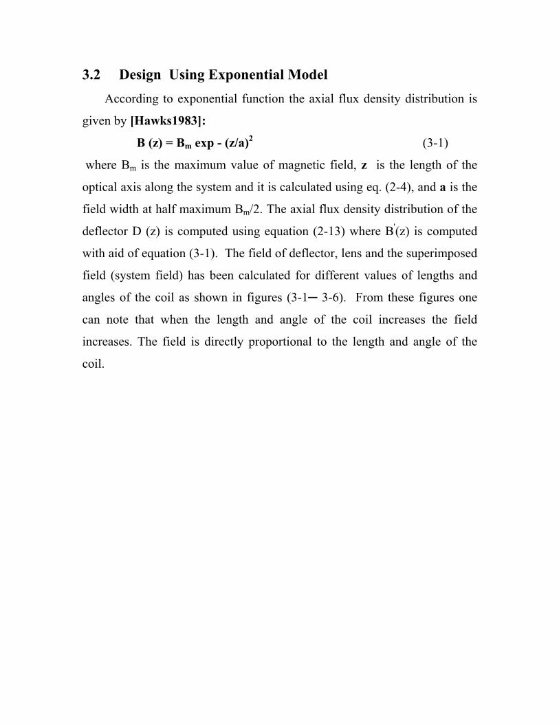
3.2 Design Using Exponential Model According to exponential function the axial flux density distribution is

iven by [Hawks1983]:

and it is calculated using eq. (2-4), and a is the

a the

g

B (z) = Bm exp - (z/a)2 (3-1)

where Bm is the maximum value of magnetic field, z is the length of the

optical axis along the system

field width at half m ximum Bm/2. The axial flux density distribution of'deflector D (z) is computed using equation (2-13) where B(z) is computed

with aid of equation (3-1). The field of deflector, lens and the superimposed

field (system field) has been calculated for different values of lengths and

angles of the coil as shown in figures (3-1─ 3-6). From these figures one

can note that when the length and angle of the coil increases the field

increases. The field is directly proportional to the length and angle of the

coil.

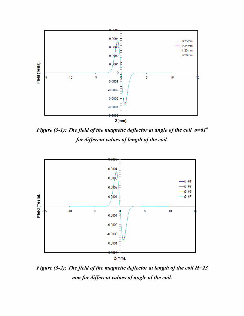
Figure (3-1): The field of the magnetic deflector at angle of the coil ø=61o

for different values of length of the coil.

Figure (3-2): The field of the magnetic deflector at length of the coil H=23

mm for different values of angle of the coil.

Figure (3-3): The field of the magnetic lens at angle of the coil ø=61o for

different values of length of the coil.

Figure (3-4): The field of the magnetic lens at length of the coil H=23 mm

for different values of angle of the coil.

Figure (3-5): The field of the magnetic system at angle of the coil ø=61o

for different values of length of the coil.

Figure (3-6): The field of the magnetic system at length of the coil H=23

mm for different values of angle of the coil.

3.3 Electron Beam Trajectory The electron beam path along the magnetic system field under infinite

magnification condition has been computed using equation (2-1). Figures (3-

7) and (3-8) shows the trajectories of an electron beam traversing the

magnetic system field at various values of both length and angle of the coil.

Figure (3-7): The electron beam trajectory in the magnetic system under

infinite magnification condition at NI/(Vr)0.5=32.27 for the angle of the

coil ø=61o and different values of length of the coil H.


infinite magnification condition at NI/(Vr)0.5=32.27 for the length of the

coil H=23mm and different values of angle of the coil ø.

Figure (3-9): The electron beam trajectory in the magnetic system

under zero magnification condition at NI/(Vr)0.5=32.27 for the angle of the

coil ø=61o and different values of length of the coil H.


zero magnification condition at NI/(Vr)0.5=32.27 for length of the coil

H=23 mm and different values of angle of the coil ø .

The effect of the length and angle of coil has been investigated at value of

excitation parameter NI/(Vr)0.5(=32.27Amp.turns/(volt)0.5. Computation has

shown that as the beam emerges from magnetic field it diverges away from

the optical axis. The trajectories of electron beams are deflecting more away

from the optical axis as the values of length of the coil (H) and angle of the

coil (Ø) decreases. The effect of change the length of the coil (H) and angle

of the coil (Ø) on the electron beam trajectory is due to the effect of the field

of the magnetic system, where as length of the coil (H) and angle of the coil

(Ø) decrease the field decreasing too as shown in figures (3-5) and (3-6).

Figure (3-9) and (3-10) shows the trajectory of an electron beam

traversing the magnetic field of the system at various values of the length of

the coil (H) and angle of the coil (Ø). These trajectories have been

computed with the aid of equation (2-1) under zero magnification condition

and the constant value of the excitation parameter NI/(Vr)0.5 = 32.27 Amp.

turns/(volt)0.5. The computation shows that the beam emerges from system

field converges near the optical axis. The trajectories of electron beams are

deflect near the optical axis as the values of length of the coil (H) and angle

of the coil (Ø) increases. The effect of changing the length of the coil (H)

and the angle of the coil (Ø) on the electron beam trajectory is due to the

effect of the magnetic field , where as length of the coil (H) and angle of the

coil(Ø) increases the field is increasing too as shown in figures (3-5) and (3-

6).

3.4 Infinite Magnification Condition

3.4.1 Effects of changing the length

a- Relative spherical and chromatic aberration coefficients

To study the effects of variation of the length of the coil (H) on the

spherical and chromatic aberration coefficients and the

different values of the length of the coil H=23, 24, 25 and 26mm with angle

of the coil Ø = 61o are taken into account. Figure (3-11) shows this effect on

the spherical aberration coefficient. This figure shows that the length

H=23mm gives the lower value of spherical aberration coefficient .

/sC f o /cC f o

/sC f o

Figure (3-11): The relative spherical aberration coefficient Cs /fο as a

function of NI/(Vr)0.5 for the angle of the coil ø=61o and the lengths of the

coil H= 23, 24, 25 and 26 mm.

Figure (3-12) shows the effect of variation of the length of the coil (H)

on the chromatic aberration coefficient . Figure (3-12) shows that

the length of the coil H =23mm gives the best value of chromatic aberration

coefficient . In both spherical and chromatic aberration coefficients

one can find that the values of relative aberration coefficient increase as the

ratio of the excitation parameter NI/(Vr)0.5 increases. Also, at the lower

values of the excitation parameter NI/(Vr)0.5 one has the best values of both

spherical and chromatic aberration coefficients , and one can select the

values of NI and Vr to keep this ratio small.

/cC f o

/cC f o

Figure (3-12): The relative chromatic aberration coefficient Cc /fο as a


coil H= 23, 24, 25 and 26 mm.

The relation between spherical and chromatic aberration coefficients

and and the length of the coil (H) is shown for the excitation

parameter NI/(Vr)0.5 =32.27 Amp. turns/(volt)0.5 in figures (3-13) and (3-14),

respectively. The values of spherical and chromatic aberration coefficients

and increase when the length of the coil (H) increases and at

the length H=23mm one can find the best result. Therefore, to reduce the

values of relative spherical and chromatic aberration coefficients the

designer can use the shorter lengths to design the toroidal deflection coil.

/sC f o

/

/cC f o

sC f o /cC f o

Figure (3-13): The relative spherical aberration coefficient Cs/fο as a

function of the coil length (H) for the angle of the coil ø=61o.



b- Relative radial and spiral distortion coefficients

Figure (3-15) shows the relative radial distortion coefficient Drad*fp2 of

the magnetic system as a function of the excitation parameter NI/(Vr)0.5.

From the figure (3-15) one can note the values of the relative radial

distortion coefficients Drad*fp2 are decreasing as the length of coil (H)

decreases. Also the values of the relative radial distortion coefficients

Drad*fp2 increase as the excitation parameter NI/(Vr)0.5 increases. The best

values of the radial distortion coefficients Drad*fp2 occur at the low values of

the excitation parameter NI/(Vr)0.5 and the length of the coil H = 23 mm

and ø=61o gives the minimum values of the aberration coefficients.

Figure (3-15): The relative radial distortion coefficient Drad *fp

2as a


coil H= 23, 24, 25 and 26 mm.

The effect of changing the length of the coil (H) on spiral distortion

coefficient is shown with different values of length of the coil H= 23, 24, 25,

and 26 mm, this effect appears in figure (3-16). The calculations show that

the coil length H = 23mm gives us the lower value of relative spiral

distortion coefficient Dsp*fo2. The values of relative radial distortion

coefficient Dsp*fo2 increase as the values of the excitation parameter

NI/(Vr)0.5 increase.

Figure (3-16): The relative spiral distortion coefficient Dsp*fο2as a

function of NI/(Vr)0.5 for the length of the coil ø=61o and lengths of the

coil H= 23, 24, 25 and 26 mm.

The relation between radial and spiral distortion coefficient Drad*fp2and

Dsp*fp2 with the length of the coil is shown in figures (3-17) and (3-18). In

these two figures, one can find that the values of radial and spiral distortion

coefficient Drad*fp2 and Dsp*fo

2increase as the length of coil increases.

Figure (3.17): The relative radial distortion coefficient Drad *fp

2 as a

function of the coil length(H) for the angle of the coil ø=61o .

Figure (3.18): The relative spiral distortion coefficient Dsp *fο2 as a

function of the coil length (H) for the angle of the coil ø=61o .

3.4.2 Effects of changing the angle


The effect of changing the angles of the coil (Ø) on the spherical and

chromatic aberration coefficients is investigated and following angles Ø =

61o, 63o, 65o, and 67o of coil, with coil length H = 23mm, are taken into

account of aberration coefficients. Figure (3-19) shows the relation between

relative spherical aberration coefficient and the excitation parameter

NI/(Vr)0.5 .This figure shows that Ø = 61o gives the lower values of spherical

aberration coefficient . Also the relative spherical aberration

coefficient increases with increasing the excitation parameter NI/(Vr)0.5.

/sC f o

/sC f o


function of NI/(Vr)0.5 for the length of the coil H= 23mm and the angle of

the coil ø=61o, 63o, 650, and 67o.

Figure (3-20) shows the relation between chromatic aberration

coefficient and the excitation parameter NI/(Vr)0.5. From the figure /cC f o

the angle of the coil Ø = 61o gives us the minimum value of chromatic

aberration coefficient and the lower values of the excitation

parameter NI/(Vr)0. give us the best values of the relative chromatic

aberration coefficient. From the calculations two parameters can be used to

reduce the spherical and chromatic aberration coefficients by selection the

best angle and the best value of the ratio of the excitation parameter

NI/(Vr)0.5 ( by changing NI and Vr).

/cC f o




The relation between spherical and chromatic aberration coefficient and with the angle of the coil (Ø) is shown in figures (3-21)

and (3-22), respectively at the excitation parameter NI/(Vr)0.5 = 32.27 Amp.

turns/(volt)0.5. Both cases have the same behavior, where the spherical and

chromatic aberration coefficient and decrease as the angle of

the coil decreases.

/sC f o /cC f o

/sC f o /cC f o


function of the angle of the coil (ø) for the length of the coil

Figure (3.22): The relative chromatic aberration coefficient Cc /fο as a

function of the angle of coil (ø) for the length of the coil H=23 mm.

b- Relative radial and spiral distortion coefficients Different angles, ø=61o, 63o, 65o, and 67o, of the coil are taken in

computation the radial and spiral distortion coefficients. Figure (3-23)

explain the results of these calculations. In this figure, the values of the

radial distortion coefficients Drad*fp2 decreases as the excitation parameter

NI/(Vr)0.5 decreases. Also, the angle of the coil Ø = 61o and lower values

the ial

of

excitation parameter NI/(Vr)0.5 gives us the lower value of relative rad

distortion coefficient Drad*fp2 .


2 as a



Figure (3-24) explain the relation between the spiral distortion

coefficients with the excitation parameter NI/(Vr)0.5. From the calculations

of four angles one can find that the minimum values of relative spiral

disto 2 o of

rtion coefficient Dsp*fo occur at angle Ø = 61 and the lower value

the excitation parameter NI/(Vr)0.5.

Figure (3-24): The relative spiral distortion coefficient Dsp*fo

2 as a

nction of NI/(Vr)0.5 for the length of the coil H= 23mm and the angle offu


The relation between the radial and spiral aberration coefficients

Drad*fp2 and Dsp*fo

2with the angle of coil (Ø) is shown in figures (3-25) and

(3-26), respectively with the excitation parameter NI/(Vr)^0.5 = 32.27 Amp.

turns/(volt)0.5. In both cases the radial and spiral aberration coefficient

Drad*fp2 and Dsp*fo

2increases as the angle increases.

Figure (3.25): The relative radial distortion coefficient Drad *fp

2 as a

function of the angle of the coil (ø) for the length of the coil H=23 mm.

Figure (3.26): The relative spiral distortion coefficient Dsp*fo2 as a

function of the angle of the coil (ø) for the length of the coil H=23 mm.

3.5 Zero Magnification Condition

3.5.1 Effects of changing the length

a-Relative spherical and chromatic aberration coefficients

variation of the length of the coil has been studied to find the

optimum length of the coil which gives us the m um values of spherical

and chromatic aberration coeff

The

inim

icients under zero magnification condition.

The calculations for different values of the length of the coil, H = 23, 24, 25,

and 26mm, are made for the angle of the coil Ø = 61o. Figure (3-27) shows

the results of spherical aberration coefficients. In this figure one can find that

the length of the coil H = 23mm gives the lower values of spherical

aberration coefficient at lower value of excitation parameter

NI/(Vr)0.5.

and t

coil H= 23, 24, 25 and 26 mm.

/sC f o


function of NI/(Vr)0.5 for the angle of the coil ø=61o he length of the

The effect of variation of the coil length on the relative chromatic

aberration coefficient is shown in figure (3-28). One finds that at the length

of the coil H = 23mm gives the best value of spherical aberration coefficient

at lower value of excitation parameter NI/(Vr)0.5 . One can note that

the relation from the figure is linear between and the length of the

coil H.


function of NI/(Vr)0.5 for the angle of the coil ø=61o and the length of the

coil H= 23, 24, 25 and 26 mm.

The relation between spherical and chromatic aberration coefficients

and with the length of the coil (H) is shown in the figures

(3-29) and (3-30), respectively at con he excitation parameter 0.5 p. turns/(volt) .5 . The values of spherical and

e

/cC f o

/cC f o

/sC f o /cC f o

stant value of t0NI/(Vr)

ch

=32.72 Am

romatic aberration coefficients and increase when th/sC f o /cC f o

length of the coil increases and the length of the coil H = 23mm gives us the



Figure (3-30): The efficient Cc /fο as a


lower values.

relative chromatic aberration co


The different values of length of the coil, H= 23, 24, 25, and 26 mm with

the angle of the coil ø=61o, are studied to find the optimum length which

give us the best values of radial and spiral distortion coefficient Drad*fp2 and

Dsp*fo2. The results of radial distortion are shown in figure (3-31). In this

figure, the length of the coil H = 23mm represent the optimum length. The

effect of changing the length of the coil on spiral distortion is shown in

figure (3-32). In this figure it appears that the length of the coil H =23mm

gives the best result. Both radial and spiral distortion aberration coefficients

have the same relation with the length of the coil, where the relative radial

and spiral distortion coefficients increase as the length of the coil increase

and this relation appears in figures (3-33) and (3-34).


2as a

function of NI/(Vr)0.5 for the angle of the coil ø=61o and the length of the

coil H= 23, 24, 25 and 26 mm.

Figure (3-32): The relative spiral distortion coefficient Dsp *fο2as a

fun e


ction of NI/(Vr)0.5 for the angle of the coil ø=61o and the length of th

coil H= 23, 24, 25 and 26 mm.

Figure (3-33): The relative radial distortion coefficient Drad *fp2 as a

Figure (3.34): The relative spiral distortion coefficient Dsp *fο2 as a


3.5.2 Effects of changing the angle

o o o o

coil H = 23mm, are used in calculations to study the effect of changing the

berration coefficient

creases when the ratio of the excitation parameter NI/(Vr)0.5 increases.


Different angles of coil, Ø = 61 , 63 , 65 and 67 with constant length of

angle of the coil on both spherical and chromatic aberration coefficients.

Figure (3-35) shows the relation between spherical aberration coefficient

and the excitation parameter NI/(Vr)0.5. In this figure, the angle of the

coil Ø = 61o give the lower value of aberration coefficients. From the figure

one can also see that the quotient spherical a

/sC f o

/sC f o

in

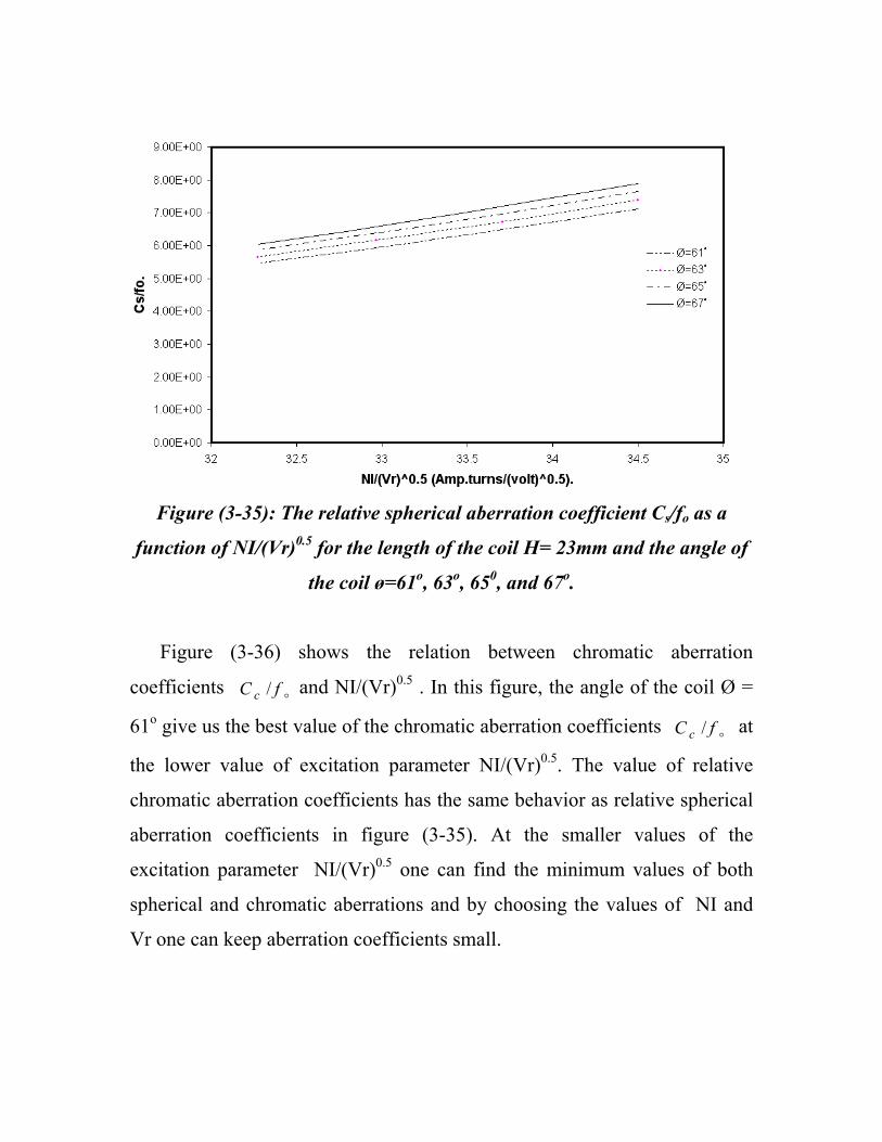
function of NI/(Vr)0. m and the angle of


3-36) s th

itation parameter

(3-3 t the

m values of both

spherical and chromatic aberrations and by choosing the values of NI and

Vr one can keep aberration coefficients small.


5 for the length of the coil H= 23m

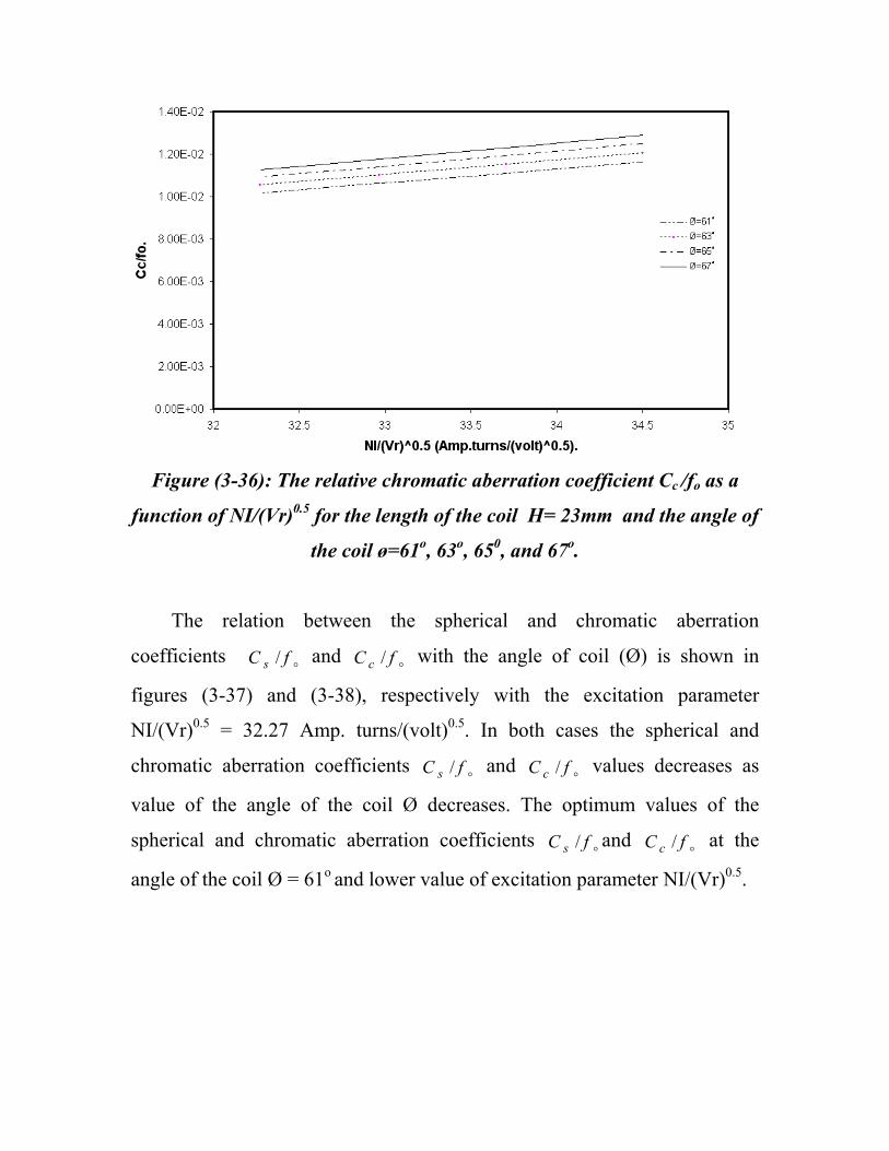
Figure ( show e relation between chromatic aberration

coefficients and NI/(Vr)0.5 . In this figure, the angle of the coil Ø =

61o give us the best value of the chromatic aberration coefficients at

the lower value of exc NI/(Vr)0.5. The value of relative

chromatic aberration coefficients has the same behavior as relative spherical

aberration coefficients in figure 5). A smaller values of the

excitation parameter NI/(Vr)0.5 one can find the minimu

/cC f o

/cC f o

F

fu f


The relation between the spherical and chromatic aberration

oefficients and with the angle of coil (Ø) is shown in

ely with the excitation parameter

NI/(Vr)0.5 p. volt . In both cases the spherical and

and values decreases as

values of the

and at the

angle of the coil Ø = 61o and lower value of excitation parameter NI/(Vr)0.5.

igure (3-36): The relative chromatic aberration coefficient Cc /fο as a

nction of NI/(Vr)0.5 for the length of the coil H= 23mm and the angle o

c /sC f o /cC f o

figures (3-37) and (3-38), respectiv

= 32.27 Am

chromatic aberration coefficients

value of the angle of the coil Ø d

spherical and chromatic aberrati

turns/( )0.5

/

ecreases. The optimum

on coefficients

sC f o /cC f o

/sC f o /cC f o

gure (3-37): The relative spherical aberration coefficient Cs/fο as a

function of the angle of the coil (ø) for the length of the coil H=23mm.

Figure (3-38): Th efficient Cc /fο as

afunction of the angle of the coil (ø) for the length of the coil H=23 mm.

Fi

e relative chromatic aberration co


The different angles of coil, Ø = 61o, 63o, 65o and 67o with constant

length of coil H = 23mm, are used in calculations to study the effect of

changing of the angle of the coil on both radial and spiral distortion

coefficients. Figure (3-39) shows the relation between radial distortion

coefficients Drad*fp2 and NI/(Vr)0.5. In this figure, the angle of the coil Ø =

61o gives the optimum value of radial distortion coefficients Drad*fp2 . Also

the ratio of the radial distortion coefficients Drad*fp2 increases as the

excitation parameter NI/(Vr)0.5 increases.

e coil ø=61o, 63o, 650, and 67o.


2 as a


th

Figure (3-40) shows the relation between spiral distortion coefficients

Dsp*fo2 and NI/(Vr)0.5 for different angles of coil Ø = 61o, 63o, 65o and 67o,

respectively. In this figure, the values of spiral distortion coefficients Dsp*fo2

are reduced when the excitation parameter NI/(Vr)0.5 decreases and the

lower value of the Dsp*fo2 occur at the angle of the coil Ø = 61o.

Figure (3-40): The relative spiral distortion coefficient Dsp *fο2 as a



The relation between the radial and spiral distortion coefficient Drad*fp2

and Dsp*fo2 with the angles of coil(Ø) is shown in figures (3-41) and (3-42),

respectively at the excitation parameter NI/(Vr)0.5 = 32.27 Amp.

turns/(volt)0.5. Both cases have the same behavior, where the radial and

spiral distortion coefficient Drad*fp2 and Dsp*fo

2 are increases as the angle

of the coil Ø increases.

Figure (3-42): The relative spiral distortion coefficient Dsp *fo

2 as a

function of the angle of the coil (ø for length of the coil H=23 mm.

Figure (3.41): The relative radial distortion coefficient Drad *fp2as a

function of the angle of the coil (ø) for length of the coil H=23 mm.

)

3.

6 pole pieces Reconstruction The pole piece shape is found by using the reconstruction method with

d of equation (2-12) and figure (3-43) shows the shape of the pole piece

l Ø = 61o and the length of the coil H = 23mm. The

ure rep ent the length of the system field.

ape of the lens and

piece shape of the deflector.

Figure (3.43): The p e coil H=23 mm

ai

for the angle of the coi

parameters (L) in the fig res

In the figure the lower part represent the pole piece sh

the upper parts represent the pole

ole piece shape when the length of th

and the angle of the coil ø=61o.

ChaChapterpter FFoouurr

d Recommendations

For

Conclusions

An

Future Work

Chapter Four

Conclusions and Suggestions for Future Work

4.1 usions

one can conclude that:-

oportionate with the four coefficient

of aberrations in the cases of zero and infinite magnification conditions.

therefore the smaller size coil of t e deflection has improved the values

of aberration.

2 - The relationship between the four coefficient of aberrations and length

and angle of the coil is inversely roportional in the cases of zero and

infinite magnification conditions, therefore, provides us with the

possibility of operating the system with high efficiently in different

operation conditions of the system

3 - The field is increasing as the values of angle and length of the coil

increases.

4- The aberration coefficients are directly proportional to the field, also the

field is increasing when the length and angle of the coil increase

therefore the aberration coefficients are increasing when the length and

angle of the coil increase.

4.2 Recommendations for Future Work

There are following topic put forward for future investigations

Concl

From the results

1 - The length and angle are inversely pr

h

p

.

(a) We recommend using different types of axial magnetic field model.

) We recommend using different types of coils as sources of magnetic

field.

(b

References

References

lamir A. S. A. (2003)

lamir A. S. A. (2004)

A

Spiral distortion of magnetic lenses with fields of the form B(z) α z-n n=2, 3

and 4 .

Optik, 114, 525-528.

A

On the chromatic aberration of magnetic lenses with a field distributio

the form of an inverse power law (B (z) α z-n).

Optik 115, 227-231.

n in

sity, Baghdad, Iraq.

aic description of beam dynamics to very high orders.

artical Accelerators, 24, 109-124.

Alamir A. S. A. (2005) On the optical properties of monopole, multipole, magnetic lenses.

Optik, 116, 429-432.

Al-Obaidi, H. N (1995) Determination of the design of magnetic electron lenses operated under

preassinged magnification conditions.

Ph.D. Thesis, Baghdad Univer

Berz M. (1989) Differential algebr

P

Bohumila L. (1988) On the design of electron beam deflection systems.

Optik, 79, 1-12.

Egerton R.f. (2007) Physical principles of electron microscopy an introduction to TEM,

and AEM .

SEM,

iley: Canada).

ign of focused ion beam for a lithography system.

h.D. Thesis, Al-Nahrain University, Baghdad, Iraq.

is.

aylor and Francis: USA and Canada.

le-aperture projection and scanning system for electron

eam.

(W

Fadhil A. Ali (2006)

Computer – aided - des

P

Goodhew, Humphreys and Beanland (2001) Electron Microscopy and Analys

T

Goto, E. , Soma, T., and Idesawa, M. (1978)

Design of a variab

b

J. Vac. Sci. Technol. 15, 883

Goto, E. and Soma, T. (1977)

ptik, 48, 255.

O

Hajime O. (1978) Moving objective lens and the Fraunhofer condition for pre-deflection.

Optik, 53, 63-68.

erlin Heidelberg new York

London).

umphries, S.Jr. (1999)

Hawkes (1982) Magnetic electron Lenses.

MSpringer-Verlag B

Hawkes P.W. (1982)

Magnetic Electron lenses.

(Springer-Verlag).

Hawkes P.W. and Kasper E. (1989)

Principles of electron optics vol.1.

(Academic press:

Hu K. and Tang TT (1999)

Lie algebra deflection aberration theory for magnetic deflection systems.

Optik, 110, 9-14.

H

Principle of charged particle acceleration.

(Wiley: New York)

Humphries, S.Jr. (2002) Charged particle beams.

(Wiley: New York).

Jiye, X. (1981)

On the linear transformations for Gaussian trajectory parameters in the combined

electron optical systems.

Optik, 59, 237-249.

Karries T. (2004)

Numerical Analysis Using MATLAB and Spreadsheets.

(Wiley: New York)

uroda, K. (1980)

uroda, K., Ozasa S. and Komoda K. (1983)

Kreyszig, E. (1983) Advance engineering mathematics.

(Wiley: Canada).

KSimplified method for calculating deflective aberration of electron optical system with

tow deflectors and lens.

Optik, 57, 251-258.

KA simplified focusing and deflection system with vertical beam landing.

J. Vac. Sci. Technol. B1, 1303-1306.

Lencova B. (1997) Electrostatic Lenses.

Handbook of Charged Particle Optics.

Edited by J. Orloff, 1

77- 222.

POC, Brno.

Lencova B. and Wisselink G. (2001) MLD (Magnetic Lens Design).

Particle Optics Group, TU Delft and S

Lencova, B.(1988)

On the design of electron beam deflection systems .

Optik, 79, 1-12.

Li Y., Kuangs S., Fen Z. and Liu T. (1993)

The relativistic fifth-order geometrical aberrations of a combined focusing-deflection

system.

J. Phys. D, Appl. Phys. 26, 522.

Liping W., John R., Haoning L., Eric M. and Xieqing Z. (2004) Simulation of electron optical systems by differential algebraic method

combined with hermite fitting for practical lens fields.

icroelectronic engineering, 73-74, 90-96.

Electron Physics.

M

Marton L. (1980)

Advances in Electronics and

Academic press: London

Munro E. (1974) Calculation of the optical properties of combined magnetic lenses and deflection systems

with superimposed field..

ptik, 39, 450-466.

. Phys. D10, 1437-1449.

canning systems using the moving objective lens .

. Vac. Sci. Technol. 15, 849

O

Munro E. (1975) Design and optimization of magnetic lenses and deflection systems for electron beams.

J. Vac. Sci. Technol. 12, 1146-1151.

Munro E. and Chu H. C. (1981b) Computation of fields in magnetic deflectors.

Optik, 60, 371-390.

Ohiwa H. (1977) Designing air core scanning systems comprising round lenses and saddle type deflection

coils.

J

Ohiwa, H. (1978) EDesign of electron-beam s

J

Ohiwa, H., Goto, E., and Ono, A. (1971) Electron .

ommun. Jpn., 54B, 44-51 C

Philip C. (1999) Introduction to electron beam lithography.

stitute for micromanufacturing.

for Electromagnetics and Microwaves.

iley series in Microwave and optical engineering.

rticle Optics part B pp.102.

cademic press: New York, London, Toronto, Sydney, and San Francisco.

zilagyi, M. (1988)

ritical assessment of the finite element method for calculating magnetic fields in

In

Richard C. Booton Jr (1992)

Computational Methods

W

Septier A. (1980) Applied Charge Pa

A

Steven T. Karris (2004)

Numerical Analysis using MATLAB and Spreadsheets.

(Prindle: United States of America).

Szilagi, M. (1988) Electron and ion optics.

(Pleum:New York)

S

Electron and ion optics.

(Plenum: New York).

Tahir K. (1985)

C

electron optics.

Ph.D. Thesis, University of Aston, Birmingham, UK.

Teruo H. (2002)

lectron beams and microwave vacuum electronics.

istortion in electron microscopy using an asymmetrical

riple pole piece lens.

a T. (1995)

Relationship between the fifth order aberration coefficients.

Optik, 113, 105-110.

Tsimring S.E. (2007)

E

(Wiley: Canada).

Tsuno K. and Harada Y.(1981) Elimination of spiral d

t

(J. phys. E: Sci. Instrum. 14, 955-960).

Uno Y., Morita H., Simazu N. and Hoskaw

Fifth-order aberration analysis of a combined electrostatic-magnetic focusing-deflection

system.

Nucl. Instrum. Method Phys. Res. A363, 10.

Wang L. P., Tang T. T., cheng B. J. and Cleaver J. R. A. (2002) Differential algebraic method for arbitrary-order aberration analysis of

combined electron beam focusing-deflection systems.

Optik, 113, 181-187.

Wang L.B. (2002)

Differential algebraic method for arbitrary-order aberration analysis of

combined electron bea

m focusing-deflection system.

Optik 113, 181-187

Wang

Differential algebraic theory and calculation for arbitrary high order aberrations of

electron lenses.

Optik, 111, 28

Yan R The abe

a rotating deflection field following the rotation of

Optik, 118, 569-574.

Zhuming L New method to correct eddy current in magnetic focusing-deflection system.

Microele

L.P., Tang T.T. and Cheng B.J.(2000)

5-289.

., Tiantong T., Yongfen K., and Xiaoli G.(2007) rration theory of a combined electron focusing deflection system with

the electrons.

. and Wenqi G. (2005)

ctronic Engineering, 78-79, 34-38.

الخلاصة

التقريب باستعمال نظام حرف وتبئير مغناطيسي بحث حاسوبي لتصميم تم أجراء

طريقة بأستخدام عن طريق حل معادله الشعاع المحوري . التركيبي لطريقة ألأمثليه

لنظام الحرف مسار الالكترون تم أيجاد الخواص البصرية و نيوستروم- كوتا- رنج

.شرط التكبير صفري تحت شرط التكبير الغير محدود و والتبئير المغناطيسي

تم استخدام التقريب التركيبي لطريقة ألأمثليه في الدراسة الحالية لإيجاد التصميم

ناطيسي التي تعطي اقل زيوغ كروي، لوني، الأمثل لنظام الحرف والتبئير المغ

.تشوه الحلزوني و تشوه نصف قطري

(تم استخدام ملف الانحراف الحلقي toroidal yoke deflection coil (

باستخدام الدالة تم تحديدهللمجال المغناطيسي، وكذلك توزيع المجال امصدر

زيوغ . النظام فكرة العدسة الشيئية المتحركة اعتمدت في حساب مجال. الأسيه

الانحراف، حيث غير الطول فالنظام خفض بتغيير الشكل الھندسي لمل

.والزاوية

مثل توزيع للمجال المحوري تم إيجاد شكل قطع القطب التي تعطي أباستخدام

.توزيع المجال ھذه باستخدام طريقة أعاده البناء

طول الملف يكونمعملات الزيوغ تظھر عندما بينت الحسابات بأن اقل

(H=23mm) .Ø=61o) ( وزاوية الملف

التكبير الصفري شرط إن العلاقة عكسية بين المعاملات الأربعة والطول و الزاوية في حال تي

أمكانية تشغيل المنظومة بكفاءة عالية في مختلف شروط تشغيل

وعلية فأنة يوفر لنا والغير محدد

. المنظومة

جمھورية العراق

وزارة التعليم العالي و البحث العلمي جامعة النھرين

كلية العلوم

حسابات ألأمثليه لمنظومة مغناطيسيه تتألف من حارف و عدسه

رسالة

مقدمة إلى كلية العلوم في جامعة النھرين وھي جزء من متطلبات نيل علوم الفيزياء درجة الماجستير في

قبلمن

احمد حسين علي )٢٠٠٦بكالوريوس (

باشراف الدكتور عدي علي حسين و الأستاذ المساعد الدكتور احمد كمال احمد

في

م٢٠٠٨الأول كانون ھـــ ١٤٢٩ذي الحجة

a computational optimization of magnetic system consists

Documents