a computational exploration of the second painlev e...
TRANSCRIPT

Noname manuscript No.(will be inserted by the editor)
A Computational Exploration of the Second PainleveEquation
Bengt Fornberg · J.A.C. Weideman
Received: date / Accepted: date
Communicated by Elizabeth Mansfield
Abstract The pole field solver developed recently by the authors (J. Comp. Phys.,230 (2011), 5957–5973) is used to survey the space of solutions of the secondPainleve equation that are real on the real axis. This includes well-known so-lutions such as the Hastings-McLeod and Ablowitz-Segur type of solutions, aswell as some novel solutions. The speed and robustness of this pole field solverenable the exploration of pole dynamics in the complex plane as the param-eter and initial conditions of the differential equation are varied. Theoreticalconnection formulas are also verified numerically.
Keywords Painleve transcendents · PII equation · connection formulas ·pole field solver
Mathematics Subject Classification (2010) 33E17 · 34M55 · 34M40 ·33F05
1 Introduction
The six Painleve equations were introduced a little over a century ago [28,29]. They define transcendental functions that have become firmly established
B. FornbergUniversity of Colorado, Department of Applied Mathematics, 526 UCB, Boulder, CO 80309,USA and National Institute for Theoretical Physics (NITheP), Private Bag X1, Matieland7602, South AfricaE-mail: [email protected]
J.A.C. WeidemanUniversity of Stellenbosch, Department of Mathematical Sciences, Private Bag X1,Matieland 7602, South AfricaE-mail: [email protected]

2 Bengt Fornberg, J.A.C. Weideman
in mathematical physics especially over the last few decades. The first two ofthese are defined by
PI :d2u
dz2= 6u2 + z, (1)
and
PII :d2u
dz2= 2u3 + z u+ α, (2)
where u(z) is a meromorphic function of z and α is a constant. Where it isnecessary to make explicit the dependence of the solution of PII on α, we shallwrite u = u(α; z).
For definitions of the remaining four equations in the Painleve family see [8,10,13,16], where lists of various applications can also be found. These includenonlinear wave motion (where PII arises as a reduction of the Korteweg-deVries equation for water waves [1,25,31]), combinatorics, random matricesand statistical physics (where PII appears in the well-known Tracy-Widomdistribution [33]), and electrostatic theory [21,22]. Short summaries of thehistory of the Painleve equations are given in the introductions of [13] and[16].
The pole distribution of the Painleve transcendents is an active researcharea. Not only do the poles carry physical significance in some applications,but the location of the poles in the complex plane also provides informationabout the solution characteristics (oscillations, decay) on the real line. A lot isknown about the distribution of poles as |z| → ∞, based on various asymptoticapproaches to the problem [4,13,23]. Much less is known for finite |z|, wherenumerical computation seems to be the only recourse.
Until recently, the presence of vast pole fields in the complex plane wasperceived to be a numerical challenge. The methodology presented in [14]overcomes this issue. It exploits in two key ways the fact that the solutionsare meromorphic: (i) the absence of branch-points allows for a flexible andeffective path selection strategy even through large and dense pole fields, and(ii) a “pole-friendly” Pade-based ODE stepping scheme [35] along these pathsmaintains high accuracy both when integrating near to as well as right upto poles of low order. When this new technique was applied to PI , numericalsolutions reported in [14] yielded errors on the order of 10−10 after integratingover distances as long as 104 through dense pole fields with average spacingon the order of 1.
Having established an effective numerical procedure, we are in a positionto apply it to other Painleve equations to look for solution features and forpole field patterns that have not been observed before. Here we focus on PII ,for the case α real and with u restricted to be real-valued on the real axis. Inparticular, Hastings-McLeod solutions (smooth and nonoscillatory along thereal axis), Ablowitz-Segur solutions (oscillatory and bounded), and tronquee-type solutions (featuring pole free sectors in the complex plane) are of specialinterest. A similar investigation for PIV (with both its parameters zero) isreported in [30].

A Computational Exploration of the Second Painleve Equation 3
The body of literature for numerical results of PII is not as extensive as it isfor analytical aspects, but it is growing. Solutions on the real axis are presentedin [9,10,21,22,27], and some pole fields in the complex plane, in the specialcase α = 0, are shown in [4,26]. The key difference between the present paperand earlier numerical studies is that we investigate here how these pole fieldsevolve with α. For such investigations the methodology of [14] offers speedand flexibility, which facilitate experimentation and create the possibility ofnumerical animations. A selection of these will be made available on the webpage [34].
The outline of the paper is as follows: After a brief overview of some gen-eral relations and explicit solutions in Section 2, we focus in Section 3 on polecounting diagrams and the use of our pole field solver as the main tools forsurveying the 3-parameter PII solution space (the parameter α and two initialconditions for the ODE). During this process, we come across all previouslyidentified solution types, and also find some generalizations of these. Thesegeneralizations include what we call secondary Hastings-McLeod solutions,studied in Section 3, and in the section following that also quasi-Hastings-McLeod and quasi-Ablowitz-Segur solutions. In Section 4 we also develop ef-fective approaches for calculating what we have named “k = 0 solutions” andfor numerically verifying connection formulas for arbitrary α. We concludewith some additional solution illustrations in Section 5 and final remarks inSection 6.
2 General Relations and Explicit Solutions
Although the solutions to PII cannot, in general, be expressed in terms ofclassical special functions, a few special cases are known. They are brieflysummarized in this section, in order to place the new computed solutions inthe context of existing knowledge. In addition, several series expansions areavailable. We start this section, however, by listing a few transformations thatenable the construction of new solutions from known ones.
2.1 Some useful relations
It is readily seen that solutions for ±α are connected via the symmetry trans-formation
u(α; z) = −u(−α; z). (3)
This makes it sufficient to consider only α ≥ 0, which we assume throughoutthis paper.
The Backlund transformation is
u(α+ 1; z) = −u(α; z)− 2α+ 1
2u′(α; z) + 2u(α; z)2 + z, (4)
4 Bengt Fornberg, J.A.C. Weideman
which defines a useful recurrence relation for generating solutions; see [10,Sect. 32.7],[15], [16, Sect. 19]. The prime denotes differentiation with respectto z. (A similar relation is available for u(α− 1; z) in terms of u(α; z); see [10,Sect. 32.7].) Solutions corresponding to α = 0 and 1
2 are connected via
u( 12 ; z) = 2−1/3
u′(0;−2−1/3z)
u(0;−2−1/3z), (5)
a relation that will be discussed in Section 5.2. In principle it is therefore onlynecessary to consider 0 ≤ α < 1
2 , as solutions for arbitrary α can then bereconstructed from (3) and (4) (or (5)). We shall not limit our investigationsto this fundamental interval in parameter space, however, as it is not straight-forward to see how pole locations and other solution features of u(α; z) andu(α+ 1; z) are connected by (4).
Near a pole, say at z = z0, the Laurent expansion of PII solutions followsimmediately from substitution into (2), namely
u(z) =c−1z − z0
+c0+c1(z−z0)+c2(z−z0)2+c3(z−z0)3+c4(z−z0)4+O((z−z0)5),
where
c−1 = ±1, c0 = 0, c1 = ∓z06, c2 =
∓1− α4
, c3 = γ, c4 =z072
(±1+3α);
see [2, Sect. 3.6] and [16, Sect. 17]. The only free parameters (in the infiniteexpansion) are the pole location z0, the sign choice in c−1 and the coefficientγ (first appearing in c3). All poles are therefore of first order, with residues ofeither +1 or −1. This is in contrast to the situation for PI where all poles areof second order, with strength of 1 and residue 0.
In the figures below, poles with residues +1 or −1 are denoted by dark(blue) and light (yellow) circles, respectively. Where zeros are shown, a smaller(red) square is used.
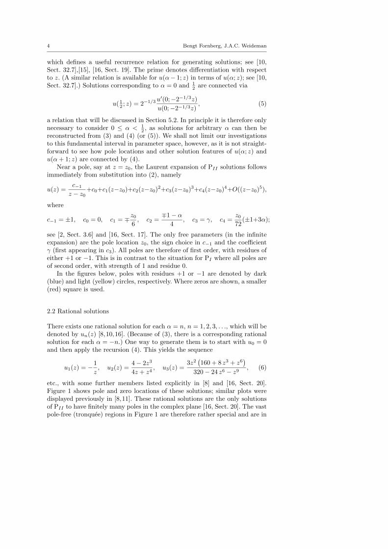
2.2 Rational solutions
There exists one rational solution for each α = n, n = 1, 2, 3, . . ., which will bedenoted by un(z) [8,10,16]. (Because of (3), there is a corresponding rationalsolution for each α = −n.) One way to generate them is to start with u0 = 0and then apply the recursion (4). This yields the sequence
u1(z) = −1
z, u2(z) =
4− 2z3
4z + z4, u3(z) =
3z2(160 + 8 z3 + z6
)320− 24 z6 − z9
, (6)
etc., with some further members listed explicitly in [8] and [16, Sect. 20].Figure 1 shows pole and zero locations of these solutions; similar plots weredisplayed previously in [8,11]. These rational solutions are the only solutionsof PII to have finitely many poles in the complex plane [16, Sect. 20]. The vastpole-free (tronquee) regions in Figure 1 are therefore rather special and are in

A Computational Exploration of the Second Painleve Equation 5
−6
−4
−2
0
2
4
6
y
n = 1 n = 2 n = 3
−6 −4 −2 0 2 4 6
−6
−4
−2
0
2
4
6
x
y
n = 4
−6 −4 −2 0 2 4 6x
n = 5
−6 −4 −2 0 2 4 6x
n = 6
Fig. 1 Poles and zeros of the first six rational solutions of PII , in the complex planez = x + iy. The dark (blue) and light (yellow) circles represent poles with residues +1 or−1, respectively. Zeros are represented by the smaller (red) squares.
fact completely destroyed by perturbations in the data (for example, changesin α or changes in the values of u(0), u′(0)).
Note in Figure 1 how the zeros of the rational solutions interlace the poles.The same thing is observed in Figure 2 of the next section. To avoid clutter,we shall therefore cease to plot zeros along with the poles from there on.
2.3 Airy solutions
There is a one-parameter family of Airy solutions when α = n + 12 , which
will be denoted by un+ 12(z) [8,10,16]. To define them, let φ be the solution to
φ′′ = − 12zφ, i.e.,
φ(z) = c1 Ai
(−z21/3
)+ c2 Bi
(−z21/3
),
with c1 and c2 arbitrary constants. Now define Φ(z) = φ′(z)/φ(z) and combinec1 and c2, by setting
c1 = cosθ
2, c2 = sin
θ
2, 0 ≤ θ ≤ 2π, (7)

6 Bengt Fornberg, J.A.C. Weideman
−8 −6 −4 −2 0 2 4 6 8
−8
−6
−4
−2
0
2
4
6
8
x
y
α = 0.5
−8 −6 −4 −2 0 2 4 6 8x
α = 1.5
−8 −6 −4 −2 0 2 4 6 8x
α = 2.5
Fig. 2 Poles and zeros of the first three Airy solutions of PII in the case θ = 0. For typicalvariation with θ, see Figure 3.
making Φ(z) 2π-periodic in the parameter θ.The Airy solution corresponding to α = 1
2 is then given by
u 12(z) = −Φ, (8)
and the others follow from (4) together with the relation Φ′(z) = − 12z−Φ(z)2.
The next two are
u 32(z) =
2Φ3 + z Φ− 1
2Φ2 + z(9)
and
u 52(z) =
4 zΦ4 + 6Φ3 + 4 z2Φ2 + 3 z Φ+ z3 − 1
(4Φ3 + 2 z Φ− 1) (2Φ2 + z), (10)
with some further members listed in [8] and [16, Sect. 21]. Because of the freeparameter θ, the Airy solutions define a much bigger family of solutions thanthe rational solutions.
Figure 2 shows locations of poles and zeros of the solutions (8)–(10), corre-sponding to the case θ = 0. These follow single lines aligned with the real axiswhen α = 1
2 , triple lines when α = 32 , etc. Figure 3 shows similar pole fields
but with θ ranging over its 2π-cycle, in the case α = 52 . Notice how five curves
of poles enter from −∞, meet up with another group of poles aligned alongthe positive real axis, and then carry with them five poles from this groupback to −∞. For the general Airy solution with α = n + 1
2 , a total of 2n + 1poles are transferred in this manner.
The pole fields displayed in Figures 1–3 were computed from explicit solu-tion formulas. In the sequel, such formulas are unavailable and all pole fieldsshown were computed with the pole field solver of [14]. The first of these isdisplayed in Figure 4, which shows pole dynamics as α is varied across [ 52 ,
72 ],
for the special case u(0) = u′(0) = 0. This sequence starts and ends withAiry solutions, with a rational solution halfway between. During the transi-tion the central group of nine poles remains relatively intact as curves of polesalternately enter from infinity, and recede back to infinity.

A Computational Exploration of the Second Painleve Equation 7
−8
−6
−4
−2
0
2
4
6
8
y
θ = 0 θ = 10−5 θ = π/3
−8 −6 −4 −2 0 2 4 6 8
−8
−6
−4
−2
0
2
4
6
8
x
y
θ = π
−8 −6 −4 −2 0 2 4 6 8x
θ = 5π/3
−8 −6 −4 −2 0 2 4 6 8x
θ = 2π − 10−5
Fig. 3 Poles of the Airy family of solutions of PII (α = 52
). Note in the θ = 13π and 5
3π cases
the exact symmetries, and also in these cases the resemblance of the central pole groups tothe rational solutions for α = 2 and α = 3, respectively. (Other cases, such as θ = 2
3π and
43π, are similar to the θ = π case in terms of lacking the 3-fold symmetry. For θ = 2π, the
solution has returned to the θ = 0 case.)
The class of solutions of PII that satisfy u(0) = u′(0) = 0 for α 6= 0 wasanalyzed in [23], where asymptotic formulas are given in the limits x → ±∞(here, and below, we use x in place of z to indicate that the variable is real).Also noted in [23] is the fact that u(3n; z) give rational solutions for n =1, 2, 3, . . ., while both u(3n − 1
2 ; z) and u(3n + 12 ; z) give Airy solutions. The
first, middle and last subplots of Figure 4 represent the n = 1 case. Similarresults hold when α is varied and the origin is a pole of either residue ±1.
Figures 3 and 4 also illustrate a type of pole behavior that is often seennear tronquee solutions of PII . As the parameter (α or θ, for example) isvaried through its critical value, curves of poles move out to infinity (leavingbehind the tronquee solution), and then move back in. At infinity, there canbe a vertical shift in alignment of the poles, which affects solution featureson either side of the tronquee case. In Figure 4, there is a tronquee solutionright in the middle (α = 3). Note the change in alignment of the poles inthe curves in the right half-plane as they move out to +∞ and back in asα is varied through the critical value 3 (cf. the middle row of subplots inFigure 4). Similar behavior is seen in Figure 3, where the first subplot (θ = 0)is a tronquee case. Note the alignment shift in the poles in the curves in the

8 Bengt Fornberg, J.A.C. Weideman
−8
−4
0
4
8
y
α = 2.5 α = 2.5001 α = 2.75
−8
−4
0
4
8
y
α = 2.9999 α = 3 α = 3.0001
−8 −4 0 4 8
−8
−4
0
4
8
x
y
α = 3.25
−8 −4 0 4 8x
α = 3.4999
−8 −4 0 4 8x
α = 3.5
Fig. 4 Poles of PII in the case u(0) = u′(0) = 0 as α is varied (in nonuniform increments)across [ 5
2, 72
]. The first and last subplots show Airy solutions, namely u 52
(z) (θ = 53π) and
u 72
(z) (θ = 13π). The middle subplot shows the rational solution u3(z).
left half-plane as θ is varied through the critical value 0 (cf. the sixth subplot,which is the same as θ = −10−5, followed by the first subplot and then thesecond).
3 Pole Counting Diagrams
The rational and the Airy solutions discussed in Section 2 are the only knownexplicit (or classical) solutions of PII . There are furthermore solutions asso-ciated with the names of Ablowitz, Boutroux, Hastings, McLeod, Segur, andothers. No expressions for these solutions in terms of known special functionsare available, however.

A Computational Exploration of the Second Painleve Equation 9
In the remainder of this paper we shall explore these and other solutionsfor α ≥ 0. Following [14,30], we base the discussion on pole counting diagrams.These diagrams display the number of poles on the positive and negative realaxes (denoted by R+ and R−, respectively) as the initial data (u(0), u′(0)) arevaried. This type of display covers for each α all possible solutions and it istherefore particularly effective in identifying and relating solutions of differenttypes, such as those referred to in the paragraph above.
A sequence of pole counting diagrams is shown in Figure 5. Initial val-ues that generate a finite number of poles along R+ define curves in the(u(0), u′(0))-plane. These are labeled n+, where n is the pole count. Whensimilarly counting poles along R−, both curves (zero width) and regions (fi-nite width) are possible. As we shall see in Section 5.1, the count n− withina region need not agree with the count along its edges. All unmarked (white)regions feature an infinity of poles along both R+ and R−.
In each diagram in Figure 5, there is a single curve marked 0+ that runsdiagonally between top left and bottom right, roughly. These 0+ curves rep-resent solutions that are pole free on R+. On either side of the 0+ curvesthere are two curves running top to bottom, labeled 1+. These denote solu-tions with a single pole on R+. The adjacent pair of curves farther out denotesolutions with two poles on R+, etc. (although we suppressed their labels toavoid clutter). The pole count increases by 1 from the inside out.
With regard to R−, there is a central curve marked 0− that runs diagonallybetween top right and bottom left, with an accompanying 0− region thatremains visible in the first five subplots in Figure 5 (but which does not vanishentirely until α = 3
2 ). These curves/regions represent solutions that are polefree on R−. Within regions marked 0−, 1−, etc., the indicated number of polesis generally followed by oscillations in u(x) as x→ −∞ (examples can be seenin Figures 12, 13, 18 and 19); the rational solutions are exceptional in that theoscillation amplitudes vanish.
In the sections below, we shall see that many of the special solutions (andfurther generalizations of these) can be identified with intersections of curvesor of curves with regions in these diagrams. For example, the intersection ofthe 0+ curves with either the 0− curves or the 0− regions, represent solutionsthat are pole free on the entire real axis. Before looking at this in more detail,we describe how the diagrams in Figure 5 were created.
Using the pole field solver of [14], we integrated PII as an initial-valueproblem, first along the interval [0, L] using a large number of initial values(u(0), u′(0)). For each set of initial values we recorded the number of poles on[0, L]. To obtain these counts, a strategy based on the residue theorem wasused. This was checked with a strategy based on computing zeros of Padedenominators. The value of L � 1 was adjusted until we reached confidencethat the pole count thus obtained is accurate for R+. The process was thenrepeated for R−.

10 Bengt Fornberg, J.A.C. Weideman
Fig. 5 Pole counting diagrams in the (u(0), u′(0))-plane. Curves labeled n+ denote initialconditions that generate solutions with n poles on R+. Curves and regions labeled n−
represent n poles on R−.
3.1 Re-visiting the rational and Airy solutions
We begin the survey of the PII solution space by noting where the explicitsolutions of Section 2 fit into the pole counting diagrams. For example, the

A Computational Exploration of the Second Painleve Equation 11
−2 −1 0 1 20
1
2
3
4
α = 1
u(0)
u′(0) 0+
1+
1+
2+
∞ 0 ↔ 1
−2 −1 0 1 2
−4
−3
−2
−1
0α = 2
u(0)
0+
1+ 2+
1+
−∞ 1 ↔ 0
Fig. 6 Extended pole counting diagrams that show (in dash-dot line type) the locationat infinity of the u1(z) and u2(z) rational solutions defined in (6). For clarity, only polecounting details for R+ are included here.
rational solution u3(z) defined in (6) is generated by initial data (u(0), u′(0)) =(0, 0). Looking at the α = 3 diagram in Figure 5, we note that the origin islocated on a 1+ curve and inside a 2− region. The one pole on R+ and twopoles on R− can be seen in the third subplot of Figure 1.
The rational solutions u1(z) and u2(z), by contrast, have poles at the originand thus (u(0), u′(0)) are both infinite. To represent such solutions, the polecounting diagrams have to be extended to infinity. Consider, for example,the rational solution u1(z) = −1/z, with u′1(z) = 1/z2. If this solution isperturbed so that this pole crosses the origin in the direction of R+, the initialdata (u(0), u′(0)) switch from (−∞,+∞) to (+∞,+∞) and the pole count onR+ increases from 0 to 1. This means that the 0+ and 1+ curves are connectedat infinity, as indicated by the dash-dot line segment in the first subplot ofFigure 6. Likewise, when the pole at z = 0 of u2(z) = (4 − 2z3)/(4z + z4) ∼1/z, z → 0, crosses the origin from left to right, the initial data switch from(+∞,−∞) to (−∞,−∞) while the pole count on R+ increases from 0 to 1.The corresponding connection is shown in the second subplot of Figure 6.
In general, if a pole of residue ±1 crosses the origin in this manner, thenu′ ∼ ∓u2 shows that the connecting curve will be at u′(0) = ∓∞ in thediagram. The relationship u′ ∼ ∓u2 also confirms the parabolic nature of thecurves where |u′(0)| � 1. In Section 5.1, similar arguments will be applied topole counts on R−.
Next, we consider the Airy solutions. Because they are one-parameter fam-ilies of solutions, they define not single points but curves in the pole countingdiagrams when the parameter θ defined in (7) is varied across its 2π-cycle.Figure 7 shows two such Airy curves, superimposed on the corresponding di-agrams from Figure 5. Observe how the Airy solution curves trace out edgesthat exist in the pole counting diagrams. In the case α = 1
2 , this curve is the

12 Bengt Fornberg, J.A.C. Weideman
−0.93 −0.92 −0.91 −0.9 −0.890.15
0.16
0.17
0.18
0.19
0.2
← θ = 0
← HM
Airy
Airy
(a)
(b)
(c)
(d)
(e)
(f)
0+ 0−
0−
0−
1−
2−
0+
0+
α = 1.5
Fig. 7 The first two subplots show (in thicker line type) curves of Airy initial conditions,superimposed on the α half-integer pole counting diagrams. The third subplot shows thedetail in a small neighborhood of the θ = 0 point in the second subplot. Solutions in thisregion will be examined in more detail in Section 5.3.
−4 −2 0 2 4−6
−4
−2
0
2
4
6α = 2.5
u(0)
u′(0)
−4 −2 0 2 4
α = 3.5
u(0)−4 −2 0 2 4
α = 4.5
u(0)−4 −2 0 2 4
α = 5.5
u(0)
Fig. 8 Curves of initial conditions of Airy solutions as the parameter θ in (7) is varied overits 2π-cycle.
parabola u′(0) = u(0)2. Four additional Airy-curves, without pole countingdiagrams, are shown in Figure 8.
There is one detail in Figure 7 that deserves pointing out. In the α = 12
diagram (first subplot) there is a small but visible gap between the intersectionpoint of the 0+ and 0− curves and the Airy initial conditions correspondingto θ = 0. This gap seems to have disappeared in the α = 3
2 diagram (secondsubplot), but it still exists. This can be seen in the magnified version of thediagram shown in the third subplot of Figure 7. (The gap gets smaller still forα = 5
2 ,72 , etc.) We postpone an examination of solution features associated
with the third subplot of Figure 7 until Section 5.3.

A Computational Exploration of the Second Painleve Equation 13
0−0+
u(0)
u′(0)
α = 0
0−0+
u(0)
α = 0.25
0−0+
u(0)
α = 0.495
0−
0+
u(0)
α = 1
Fig. 9 Pole counting diagrams on [−2, 2]× [−2, 2] showing the location of Hastings-McLeodinitial conditions as dots.
3.2 Hastings-McLeod solutions
Figure 9 shows four pole counting diagrams, three of which were displayed ona larger domain in Figure 5. Only the 0+ curves and 0− curves/regions arenow shown, because our present interest is in solutions that are pole free onthe entire real axis.
When α = 0, the 0+ curve is seen to intersect the 0− region along a curvesegment that connects the two points
(u(0), u′(0)) ≈ (±0.3670615515480784,∓0.2953721054475501).
The corresponding two solutions (which, by (3), only differ in sign), are there-fore pole free and nonoscillatory on the real axis, i.e., this corresponds to thewell-known Hastings-McLeod solution [17]. When α increases from 0 the sym-metry is broken and the two dots in Figure 9 move closer together, coalescingwhen α = 1
2 . This implies that if 0 < α < 12 , then there are two (nonsymmet-
ric) solutions that are pole free and nonoscillatory on the entire real axis. Onlyone of these has been described in any detail in the literature, as a generalizedHastings-McLeod solution [3,7,13].
To distinguish between these two solutions, consider for α > 0 the asymp-totic boundary conditions [7,10,13,17,18]
u(x) ∼
{±√− 1
2x, x→ −∞;
−α/x, x→ +∞.(11)
These are obtained as asymptotic balances between the right-hand side termsin (2) when solutions are smooth and the second derivative becomes negligible,giving
2u3 + xu+ α = 0. (12)
(In the case α = 0, this argument needs refinement; see (13) and the discussionthat follows it.)
The plus and minus signs in (11) are identified with the lower and upperdots in Figure 9, respectively. Corresponding solutions in the case α = 0.495are shown in the middle subplot of the first column of Figure 10. The lower

14 Bengt Fornberg, J.A.C. Weideman
−10 0 10
−2
−1
0
1
2
α=
0
u(0) = -0.367u′(0) = 0.295
u(0) = 0.367u′(0) = -0.295
−10 −5 0 5 10−10
−5
0
5
10Primary (lower) solution
−10 −5 0 5 10−10
−5
0
5
10Secondary (upper) solution
−10 0 10
−2
−1
0
1
2
α=
0.495
u(0) = -0.637u′(0) = 0.239
u(0) = -0.612u′(0) = 0.201
−10 −5 0 5 10−10
−5
0
5
10
−10 −5 0 5 10−10
−5
0
5
10
−10 0 10
−2
−1
0
1
2
α=
1
u(0) = -0.795u′(0) = 0.203
−10 −5 0 5 10−10
−5
0
5
10
Fig. 10 Hastings-McLeod solutions and their corresponding pole fields. The thinner curvesin the first column are the branches of the cubic equation (12) that defines the asymptoticboundary conditions (11). (One of these is completely obscured behind the thick solutioncurves, but is better visible in Figures 12, 13 and 18 below.)
solution (minus sign in (11)), is pole free, nonoscillatory, and monotone, andis the solution described in [3,7,13]. The upper solution (plus sign in (11))is likewise pole free and nonoscillatory but not monotone. These features ofthe upper solution have not been noted in the literature as far as we know,although its asymptotic properties are recorded in [13, Thm. 11.7]. We refer tothese two solutions as the primary and secondary Hastings-McLeod solutions,respectively.
As α increases from 0, the primary solution changes slowly as can be seenin Figure 10. By contrast, the secondary solution develops a steep gradienton the negative real axis, which moves out to −∞ as α → 1
2 . When α = 12 ,
u ∼ −√− 1
2x as x→ −∞, and the two solutions coalesce pointwise.
The pole fields shown in the second and third columns of Figure 10 clarifythe process. They were obtained using the values of (u(0), u′(0)) for which
A Computational Exploration of the Second Painleve Equation 15
−1.5 −1 −0.5 0 0.5 1 1.5−1.5
−1
−0.5
0
0.5
1
1.5
u(0)
ks = 1
kp = −1
α = 0
u′(0)
−1.5 −1 −0.5 0 0.5 1 1.5−1.5
−1
−0.5
0
0.5
1
1.5
u(0)
ks =12
kp = −
12
α = 13
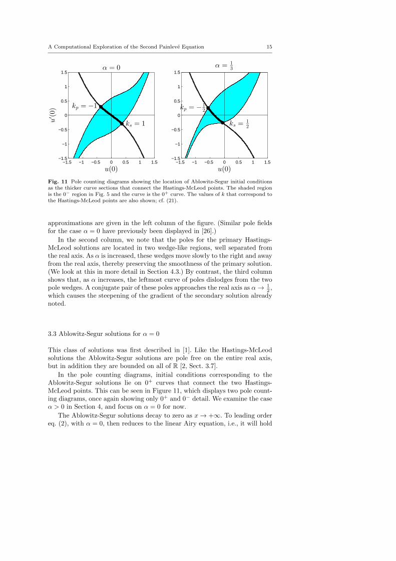
Fig. 11 Pole counting diagrams showing the location of Ablowitz-Segur initial conditionsas the thicker curve sections that connect the Hastings-McLeod points. The shaded regionis the 0− region in Fig. 5 and the curve is the 0+ curve. The values of k that correspond tothe Hastings-McLeod points are also shown; cf. (21).
approximations are given in the left column of the figure. (Similar pole fieldsfor the case α = 0 have previously been displayed in [26].)
In the second column, we note that the poles for the primary Hastings-McLeod solutions are located in two wedge-like regions, well separated fromthe real axis. As α is increased, these wedges move slowly to the right and awayfrom the real axis, thereby preserving the smoothness of the primary solution.(We look at this in more detail in Section 4.3.) By contrast, the third columnshows that, as α increases, the leftmost curve of poles dislodges from the twopole wedges. A conjugate pair of these poles approaches the real axis as α→ 1
2 ,which causes the steepening of the gradient of the secondary solution alreadynoted.
3.3 Ablowitz-Segur solutions for α = 0
This class of solutions was first described in [1]. Like the Hastings-McLeodsolutions the Ablowitz-Segur solutions are pole free on the entire real axis,but in addition they are bounded on all of R [2, Sect. 3.7].
In the pole counting diagrams, initial conditions corresponding to theAblowitz-Segur solutions lie on 0+ curves that connect the two Hastings-McLeod points. This can be seen in Figure 11, which displays two pole count-ing diagrams, once again showing only 0+ and 0− detail. We examine the caseα > 0 in Section 4, and focus on α = 0 for now.
The Ablowitz-Segur solutions decay to zero as x→ +∞. To leading ordereq. (2), with α = 0, then reduces to the linear Airy equation, i.e., it will hold

16 Bengt Fornberg, J.A.C. Weideman
thatu(x) ∼ kAi(x), x→ +∞, (13)
where k is a free parameter.The question addressed and solved in [1,3,12,13,17,24,25,31,32] and else-
where, is to find the asymptotic behavior as x → −∞ of the solution thatsatisfies (13) as x → +∞. The answer depends on k and one needs to distin-guish between |k| < 1, |k| = 1 and |k| > 1.
In the case |k| < 1, the asymptotic behavior on the negative real axis is
u(x) ∼ d(−x)1/4 sin(2
3(−x)3/2 − 3
4d2 log(−x)− θ0
), x→ −∞, (14)
where d and θ0 are constants. The connection formulas
d2 = −π−1 log(1− k2) (15)
and
θ0 =3
2d2 log 2 + argΓ
(1− 1
2id2)
+1
4π(
1− 2 sgn k)
(16)
hold when the two parts of the solution, (13) and (14), are connected smoothly.As k → ±1 it was proven in [17] that the oscillatory behavior of (14)
turns into the square root behavior u ∼ ±√− 1
2x. (This defines the Hastings-
McLeod solution, which means the second boundary condition in (11) shouldbe modified to u(x) ∼ ±Ai(x), x → +∞ in the case α = 0.) When |k| >1, poles appear on the negative real axis. (The physical significance of thevalue |k| = 1, in the water wave application, is that it distinguishes betweennonlinearity dominating dispersion and vice versa [25,31].)
Figure 12 shows solutions for values of k near the critical value 1, i.e., nearthe secondary Hastings-McLeod solution. (By (3), there exist similar solutionsnear the primary Hastings-McLeod solution, k = −1.) When k is slightly lessthan the critical value we observe an Ablowitz-Segur solution, with oscillatorytail described by (14). (In fact, when graphs of (13) and (14) are superimposedon the graph shown here, no discrepancy can be seen in the regions x > 0 andx < −3, respectively. Similar agreements were previously shown in [25,31].)When k slightly exceeds the critical value, the solution features an infinity ofpoles on R−.
Similar solutions (along the real axis) were displayed previously in [8,10,21,22]; in fact, the values k = 1±0.001 were chosen so that the solution curvesin Figure 12 match the curves in [10, Fig. 32.3.6]. The corresponding pole fieldsare displayed in the right column of Figure 12.
The pole fields consist of the wedge-like sectors already observed in Fig-ure 10, supplemented by a separate field farther into the left half-plane. Whenk is slightly less than 1 some of these poles are located just off the real axis,which causes the oscillatory features of the solution seen in the first subplotof Figure 12 and described asymptotically by (14). As k increases this fieldmoves to the left, and at the critical k = 1 it reaches z = −∞, leaving onlythe two wedges. As k increases further, the poles enter again from z = −∞,

A Computational Exploration of the Second Painleve Equation 17
−10 −5 0 5 10−10
−5
0
5
10
x
y
−10 −5 0 5 10−5
0
5
x
uk = 0.999
−10 −5 0 5 10−10
−5
0
5
10
x
y
−10 −5 0 5 10−5
0
5
x
u
k = 1.001
Fig. 12 Solutions of PII (α = 0) corresponding to two values of k in the asymptoticboundary condition u(x) ∼ kAi(x), x → +∞; cf. (17). The solution in the first subplot isan Ablowitz-Segur solution. (The in-between case, k = 1, is one of the Hastings-McLeodsolutions shown in the first subplot of Fig. 10.) The figures on the right are the pole fieldsof the solutions on the left.
but this time vertically aligned such that there are poles along the real axis.This is the familiar behavior near a tronquee solution, already noted at theend of Section 2.3.
4 Generalizations to α > 0
In addition to the primary and secondary Hastings-McLeod solutions definedin Section 3.2, we describe below a class of solutions for the case α > 1
2 ,which has the same asymptotic properties as the secondary Hastings-McLeodsolution, but with a finite number of poles on R. These will be referred toas quasi-Hastings-McLeod solutions. To keep the discussion uncluttered, weintroduce here the abbreviations pHM, sHM, and qHM for primary, secondary,and quasi-Hastings-McLeod solutions, respectively. Similarly, we abbreviatethe regular and quasi-Ablowitz-Segur solutions by AS and qAS, respectively.

18 Bengt Fornberg, J.A.C. Weideman
4.1 Refinements of the boundary condition for x→ +∞
Here we derive higher order expansions for the boundary conditions (11) and(13) that will be necessary for our numerical work. We first note that anysolution u(α;x) that is smooth for x→ +∞ can be written as
u(α;x) = B(α;x) + e(α, k;x), (17)
where B(α;x) satisfies an asymptotic series of the form
B(α;x) ∼ −αx
∞∑n=0
bnx3n
, (18)
and e(α, k;x) ∼ kAi(x) is independent of α to leading order and contains onlyexponentially small terms in x [5,6]. (The expansions (17)–(18) hold, in fact,in the sector arg x ∈ (− 1
3π,13π). This is a result due to Boutroux, who also
considered similar expansions in larger sectors but which are not real on thereal axis, and therefore outside the scope of the present paper.)
In (18), b0 = 1 and a recurrence formula for the other bn is given in [8,15].It transpires that each bn is a polynomial of degree 2n in even powers of α.
Besides this dependence on α, the function B(α;x) contains no free param-eters, while e(α, k;x) contains the additional parameter k. In the case α = 0,the function B(α;x) vanishes and (17) matches (13) in the limit x → +∞.When α = 1, 2, 3, . . ., the series (18) converges and reproduces the rationalsolutions described in Section 2.2 [9]. In this case (17) matches the type ofboundary condition considered in [2,9].
The function e(α, k;x) can likewise be expanded in the limit x→ +∞ as
e(α, k;x) ∼ k
2√π
e−(2/3)x3/2
x1/4
∞∑n=0
cnx3n/2
+
(k
2√π
)2e−(4/3)x
3/2
x4/4
∞∑n=0
dnx3n/2
+O(k3e−(6/3)x
3/2
x7/4
), (19)
with coefficients
c0 = 1, c1 =1
48
(− 5 + 96α2
), c2 =
1
4608
(385− 7872α2 + 9216α4
), etc.,
and
d0 = 0, d1 = −2α, d2 =1
12
(77α− 96α3
), etc.
These (as well as the bn) are readily generated by substituting (17) (expandedaccording to (18) and (19)) into (2) and equating coefficients.

A Computational Exploration of the Second Painleve Equation 19
4.2 Connection formulas
Connection formulas analogous to (14)–(16) for arbitrary α were derived in[20,24]. We do not reproduce these formulas here, except to note that (15)should be modified to
d2 = −π−1 log(
cos2(πα)− k2). (20)
(For the meaning of d we refer to [24].) The critical values of k that definepHM and sHM solutions are therefore
kp = − cosπα, ks = cosπα. (21)
The main challenge in verifying this theory numerically is to compute thek = 0 function B(α;x). When α is not an integer, the series (18) divergesviolently and neither truncation at the optimal point nor sequence accelera-tion can be used to compute B(α;x) accurately. This is not surprising since(18) alone, even with all the bn known, does not define B(α;x) uniquely. Theexpansion (19), however, allows this ambiguity to be bypassed, also leadingto an effective computational procedure to obtain a unique B(α;x) (for anyα > 0), which we will call the k = 0 solution.
Based on the two critical choices for k defined in (21), it follows from (17)that
up(α;x) = B(α;x) + e(α, kp;x), us(α;x) = B(α;x) + e(α, ks;x), (22)
where up(α;x) and us(α;x) are the pHM and sHM solutions. Because up(α;x)is unique and pole free along the entire real axis for every α, it is computedwithout difficulty as the solution to an ODE boundary-value problem. Theexpansion (19) provides accurate values of e(α, kp;x) and e(α, ks;x) and theirx-derivatives at sufficiently large x = X. Using, for example, c0, c1, . . . , c12and d0, d1, . . . , d8, near machine accuracy is achieved with X = 8. Because(22) implies
us(α;x) = up(α;x) + e(α, ks;x)− e(α, kp;x) (23)
the sHM solution can now be obtained by initiating the pole field solver withthe now known values for the right-hand side of (23), i.e., for us(α;X) andu′s(α;X). A similar procedure is used for computing B(α;x), based on thefirst equation in (22). (We remark that in the case 0 ≤ α < 1
2 an alternativeprocedure for computing us(α;x) is to solve it as a boundary-value problem, forit too is then a pole free solution albeit not as smooth as up(α;x); cf. Figure 10.Being able to compute us(α;x) in two distinct ways offers a useful numericalcheck.)
Before we have a closer look at the solutions us(α;x) and B(α;x), let usreturn briefly to the pole counting diagram for α = 1
3 shown in the secondsubplot of Figure 11. The objective here is to verify the validity of the criticalk formula (21), which turns into kp = − 1
2 and ks = 12 in the α = 1
3 case. Theexpansion (19) was used to compute e( 1
3 , k;x) for four values near k = ± 12

20 Bengt Fornberg, J.A.C. Weideman
−10 −5 0 5 10−5
0
5
x
uk = -0.4999; -0.5001
−10 −5 0 5 10−5
0
5
x
u
k = 0.5001; 0.4999
Fig. 13 Solutions of PII (α = 13
) corresponding to four values of k in the asymptotic
boundary condition u( 13
;x) ∼ B( 13
;x)+kAi(x), x→ +∞; cf. (17). Values |k| < 12
correspond
to the smooth, oscillatory solutions (Ablowitz-Segur) and values |k| > 12
correspond to the
solutions with poles on R−.
and the corresponding solutions were computed as described in the previousparagraph.
Figure 13 shows two AS solutions corresponding to k = ±0.4999, bothoscillatory on R−. It also shows two solutions, corresponding to k = ±0.5001,which exhibit a string of poles on R−.
The HM solutions for k = ± 12 are not shown in Figure 13, but they con-
tinue to follow the shown asymptotic curves ±√−x/2 as x→ −∞. The corre-
sponding pole fields are not shown either, but they are similar to the pole fieldsshown in Figure 12. When |k| is just less than the critical value 1
2 , the polesare located just off the real axis, leading to the oscillations in u(x) on R−. Atthe critical |k| = 1
2 these poles have cleared to −∞, to reappear precisely onthe real axis when |k| just exceeds 1
2 .
4.3 Quasi-Hastings-McLeod and Quasi-Ablowitz-Segur solutions
Consider again the pole counting diagrams displayed in Figure 11 and the firstthree subplots of Figure 9. These are typical diagrams for the case 0 ≤ α < 1
2 ,with the two HM points located on two opposite edges of the 0− region, andthe connecting curve representing the AS solutions. As α increases from 0to 1
2 , the secondary point moves closer to the primary one. They are bothlocated on the 0+ curve, at opposite edges of the 0− region. The two pointscoalesce at α = 1
2 , at which time the 0− region has shrunk to zero width inthat neighborhood.
When α is increased beyond 12 , the sHM point passes through the primary
one, while continuing along the 0+ curve but now entering a 1− region. (Vi-sualize the morphing of the third subplot into the fourth in Figure 5.) Thefirst subplot in Figure 14 shows a typical case. Here α = 2
3 , with kp = 12 and
A Computational Exploration of the Second Painleve Equation 21
−4 −2 0 2 4
−8
−6
−4
−2
0
2
4
6
8
kp =12
k = 0
ks = −
12
+∞
−∞
u′(0)
α = 23
u(0)
0+1−
−4 −2 0 2 4
k = 0
kp = 1
ks = −1
α = 1
u(0)
0+1−
1+0−
−4 −2 0 2 4
k = 0
kp = −1
ks = 1
α = 2
u(0)
0+
1− 1+
2−
−4 −2 0 2 4
k = 0
ks = −1
kp = 1
α = 3
u(0)
0+
1+2−
3−
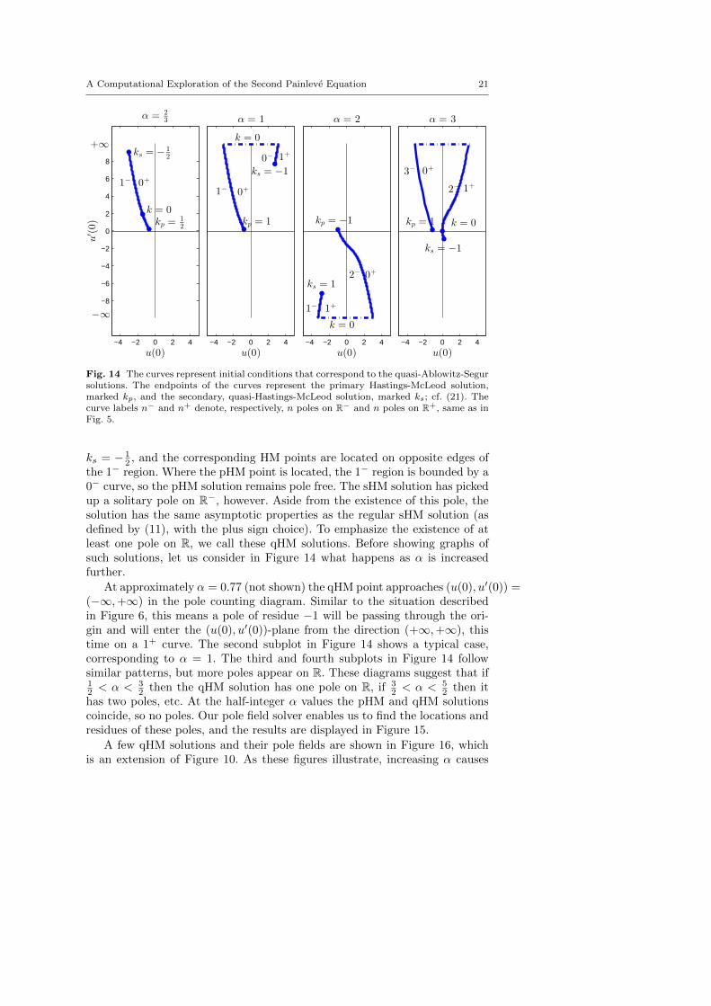
Fig. 14 The curves represent initial conditions that correspond to the quasi-Ablowitz-Segursolutions. The endpoints of the curves represent the primary Hastings-McLeod solution,marked kp, and the secondary, quasi-Hastings-McLeod solution, marked ks; cf. (21). Thecurve labels n− and n+ denote, respectively, n poles on R− and n poles on R+, same as inFig. 5.
ks = − 12 , and the corresponding HM points are located on opposite edges of
the 1− region. Where the pHM point is located, the 1− region is bounded by a0− curve, so the pHM solution remains pole free. The sHM solution has pickedup a solitary pole on R−, however. Aside from the existence of this pole, thesolution has the same asymptotic properties as the regular sHM solution (asdefined by (11), with the plus sign choice). To emphasize the existence of atleast one pole on R, we call these qHM solutions. Before showing graphs ofsuch solutions, let us consider in Figure 14 what happens as α is increasedfurther.
At approximately α = 0.77 (not shown) the qHM point approaches (u(0), u′(0)) =(−∞,+∞) in the pole counting diagram. Similar to the situation describedin Figure 6, this means a pole of residue −1 will be passing through the ori-gin and will enter the (u(0), u′(0))-plane from the direction (+∞,+∞), thistime on a 1+ curve. The second subplot in Figure 14 shows a typical case,corresponding to α = 1. The third and fourth subplots in Figure 14 followsimilar patterns, but more poles appear on R. These diagrams suggest that if12 < α < 3
2 then the qHM solution has one pole on R, if 32 < α < 5
2 then ithas two poles, etc. At the half-integer α values the pHM and qHM solutionscoincide, so no poles. Our pole field solver enables us to find the locations andresidues of these poles, and the results are displayed in Figure 15.
A few qHM solutions and their pole fields are shown in Figure 16, whichis an extension of Figure 10. As these figures illustrate, increasing α causes

22 Bengt Fornberg, J.A.C. Weideman
−8 −6 −4 −2 0 2 40
1
2
3
4
5
6
x
α
Fig. 15 Pole locations on R for the quasi-Hastings-McLeod solutions for various α. Thedash-dot and solid curves represent residues −1 and +1, respectively. The horizontal linesrepresent half-integer values of α.
the pHM pole field wedges to move smoothly to the right and away fromthe real axis. The pole fields for the sHM solution agree with these whenα = 1
2 ,32 ,
52 , etc., but Figures 14–16 indicate a fundamentally different process
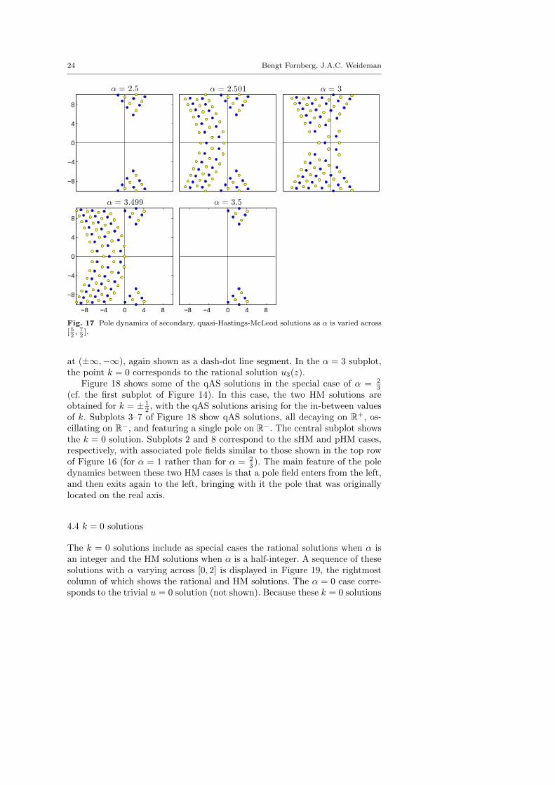
at intermediate α values. An example of this is seen in Figure 17, where α isincreased from 5
2 to 72 . A band made up of five curves of poles enters from
the left, and joins the pole wedges. As α approaches 72 , seven curves of poles
dislodge from the wedges on the left sides, and exit together towards minusinfinity (to be compared to the dislodging of the single curve of poles seen inone of the subplots of Figure 10). During this process, the HM wedges haveactually moved slightly towards the real axis and to the left, but the end resultgives the opposite impression, because its two leftmost rows of poles has gotseparated off and transported out to minus infinity. Throughout this process,the pole configuration along the real axis remains reminiscent of the one forthe rational solution at α = 3, sliding in from the left and then returning outto the left again.
As noted by [19], the characteristics of the qHM solutions can be partiallyexplained by the Backlund transformation (4). Consider the second boundarycondition in (11): if u(α;x) ∼ −α/x, x → +∞, is substituted into the right-hand side of (4) one gets u(α+1;x) ∼ −(α+1)/x, i.e., this boundary conditionis preserved by the transformation. The first boundary condition in (11), ex-tended by one term, reads u(α;x) ∼ ±
√−x/2 +α/(2x) + . . ., x→ −∞. Then
(4) produces u(α+1;x) ∼ ∓√−x/2, i.e., this boundary condition is preserved
but for a sign change. That is, the upper solution u(α;x) maps to the lowersolution u(α + 1;x) and vice versa. Next, check the sign of the denominatorin (4), say v = 2u′ + 2u2 + x, in the limits x → ±∞. When the plus sign is

A Computational Exploration of the Second Painleve Equation 23
−5 0 5
−5
0
5
α=
1
u(0) = -0.795u′(0) = 0.203
u(0) = 2.746u′(0) = 7.699
−5 0 5
−5
0
5
Primary (smooth) solution
−5 0 5
−5
0
5
Secondary (singular) solution
−5 0 5
−5
0
5
α=
2
u(0) = -1.000u′(0) = 0.165
u(0) = -2.844u′(0) = -7.148
−5 0 5
−5
0
5
−5 0 5
−5
0
5
−5 0 5
−5
0
5
α=
3
u(0) = -1.145u′(0) = 0.145
u(0) = 0.184u′(0) = -0.906
−5 0 5
−5
0
5
−5 0 5
−5
0
5
Fig. 16 Same as Fig. 10, but now including the quasi-Hastings-McLeod solutions. Thesesolutions have the same asymptotics as the regular Hastings-McLeod solutions as x→ ±∞,but they have one or more poles on R.
considered in (11), v is negative in both x limits but when the negative signis considered v has opposite signs. This sign change in the denominator of (4)makes it plausible that the secondary HM solution picks up an additional poleon the real axis when the value of α is increased by one. A proof that one andonly one pole is added in this manner will require a deeper analysis, however.
The curves in Figure 14 represent values of k between kp and ks, and areassociated with solutions similar to the regular AS solutions (oscillatory asx → −∞, smoothly decaying as x → +∞), except for the existence of polesin between. We refer to these as qAS solutions (previously noted in [2] in thespecial case of integer α). They coincide with the pHM solution when α ishalf-integer. Otherwise, like the qHM solutions they have [α + 1
2 ] poles alongR (where [ · ] denotes the integer part).
In the α = 1 case in Figure 14, the k = 0 point is located at (±∞,+∞) inthe diagram, as indicated by the dash-dot line segment. This is the rationalsolution u1(z), defined in (6) and displayed in a pole counting diagram inFigure 6. Similarly, in the α = 2 subplot, the rational solution u2(z) is located
24 Bengt Fornberg, J.A.C. Weideman
−8
−4
0
4
8
α = 2.5 α = 2.501 α = 3
−8 −4 0 4 8
−8
−4
0
4
8
α = 3.499
−8 −4 0 4 8
α = 3.5
Fig. 17 Pole dynamics of secondary, quasi-Hastings-McLeod solutions as α is varied across[ 52, 72
].
at (±∞,−∞), again shown as a dash-dot line segment. In the α = 3 subplot,the point k = 0 corresponds to the rational solution u3(z).
Figure 18 shows some of the qAS solutions in the special case of α = 23
(cf. the first subplot of Figure 14). In this case, the two HM solutions areobtained for k = ± 1
2 , with the qAS solutions arising for the in-between valuesof k. Subplots 3–7 of Figure 18 show qAS solutions, all decaying on R+, os-cillating on R−, and featuring a single pole on R−. The central subplot showsthe k = 0 solution. Subplots 2 and 8 correspond to the sHM and pHM cases,respectively, with associated pole fields similar to those shown in the top rowof Figure 16 (for α = 1 rather than for α = 2
3 ). The main feature of the poledynamics between these two HM cases is that a pole field enters from the left,and then exits again to the left, bringing with it the pole that was originallylocated on the real axis.
4.4 k = 0 solutions
The k = 0 solutions include as special cases the rational solutions when α isan integer and the HM solutions when α is a half-integer. A sequence of thesesolutions with α varying across [0, 2] is displayed in Figure 19, the rightmostcolumn of which shows the rational and HM solutions. The α = 0 case corre-sponds to the trivial u = 0 solution (not shown). Because these k = 0 solutions

A Computational Exploration of the Second Painleve Equation 25u
k = -0.501 k = -0.5 k = -0.499
u
k = -0.25 k = 0 k = 0.25
x
u
k = 0.499
x
k = 0.5
x
k = 0.501
Fig. 18 Solutions of PII (α = 23
) corresponding to nine values of k in the asymptotic
boundary condition u(x) ∼ B(x) + kAi(x), x→ +∞; cf. (17). Values |k| < 12
correspond to
quasi-Ablowitz-Segur solutions, k = 12
corresponds to the regular Hastings-McLeod solution,
and k = − 12
to a quasi-Hastings-McLeod solution. Values |k| > 12
feature an infinity of poles
on R−. (All solutions are displayed on [−8, 8]× [−10, 10].)
are special cases of qAS solutions, they show the familiar pattern of oscilla-tions on R−, decay on R+, and [α+ 1
2 ] poles along R. (The exceptions are theα integer cases, where the oscillations are not present, and the α half-integercases, where neither oscillations nor poles are present.)
We continue our display of k = 0 solutions in Figure 20, but now showingpole fields instead as α varies across [2, 3]. All these solutions are pole free inlarge sectors of the right half-plane, and therefore of tronquee-type. Observealso how the group of four poles associated with the rational solution u2(z)move along the negative real axis as α is increased, and disappears to −∞as α → 5
2 . As α is increased further, the group of nine poles associated withthe rational solution u3(z) enters from the left, and settles in a symmetricconfiguration around the origin as α→ 3.

26 Bengt Fornberg, J.A.C. Weideman
α = 0.1 α = 0.25 α = 0.33333 α = 0.49 α = 0.5
α = 0.51 α = 0.66667 α = 0.75 α = 0.9 α = 1
α = 1.1 α = 1.25 α = 1.3333 α = 1.49 α = 1.5
α = 1.51 α = 1.6667 α = 1.75 α = 1.9 α = 2
Fig. 19 k = 0 solutions as α is varied (in nonuniform increments) across [0, 2]. In therightmost column these solutions reduce to the rational solutions in the case α integer, andto the Hastings-McLeod solutions in the case α half-integer. (All solutions are displayed on[−10, 6]× [−4, 4].)
5 Additional Solution Illustrations
5.1 Pole counting diagrams: domain edges and poles crossing the origin
When we follow a family of solutions for which a pole passes the origin, wenoted in Section 3.1 (cf. Figure 6) how the corresponding initial conditionsat z = 0 would be affected. These were seen to follow trajectories in the(u(0), u′(0))-plane, which connect at either u′(0) = +∞ or u′(0) = −∞ ac-cording to if the pole passing the origin has residue −1 or +1. If finite, boththe counts n+ and n− change by one. When counting poles on R+, the regionswith finite count n+ always form curves (of zero width) in the pole countingdiagrams.
Turning to similar counts on R−, Figure 5 showed that finite counts n− canoccur also within entire regions, not only along curves. Additionally, the countsalong the edges of these regions need not agree with counts for within theregions. As an example, the left subplot of Figure 21 shows all these differentcounts for R− and the associated connection lines in the case of α = 3. Theright subplot of that figure shows corresponding pole counts on R+.

A Computational Exploration of the Second Painleve Equation 27
−8
−4
0
4
8
α = 2 α = 2.01 α = 2.4
−8
−4
0
4
8
α = 2.49 α = 2.5 α = 2.51
−8 −4 0 4 8
−8
−4
0
4
8
α = 2.6
−8 −4 0 4 8
α = 2.99
−8 −4 0 4 8
α = 3
Fig. 20 Pole dynamics for the k = 0 solutions as α is varied across [2, 3].
The α half-integer cases reveal still an additional feature in that some ofthe n− regions join each other side-to-side, whereas others lose their width andturn into n− curves. Figure 22 gives the different n− counts and connectionlines in such a case (α = 3
2 ; cf. also the last two subplots in Figure 7).In all cases, there is (at least) one 0− curve between bottom left and top
right in the pole counting diagrams (either as a domain boundary or, in thehalf-integer cases, partly a domain boundary) and also a single 0+ curve be-tween bottom right and top left. As discussed in more detail already, thisensures the existence of Hastings-McLeod solution(s) for all α.
5.2 Relating u(0; z) and u( 12 ; z) solutions
Here we consider the connection between α = 0 and α = 12 solutions as
described by (5). It follows from that representation that both poles and zerosof u(0; z) can generate poles of u( 1
2 ; z).
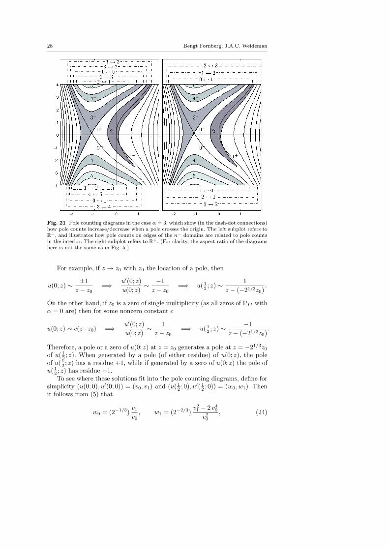
28 Bengt Fornberg, J.A.C. Weideman
Fig. 21 Pole counting diagrams in the case α = 3, which show (in the dash-dot connections)how pole counts increase/decrease when a pole crosses the origin. The left subplot refers toR−, and illustrates how pole counts on edges of the n− domains are related to pole countsin the interior. The right subplot refers to R+. (For clarity, the aspect ratio of the diagramshere is not the same as in Fig. 5.)
For example, if z → z0 with z0 the location of a pole, then
u(0; z) ∼ ±1
z − z0=⇒ u′(0; z)
u(0; z)∼ −1
z − z0=⇒ u( 1
2 ; z) ∼ 1
z − (−21/3z0).
On the other hand, if z0 is a zero of single multiplicity (as all zeros of PII withα = 0 are) then for some nonzero constant c
u(0; z) ∼ c(z−z0) =⇒ u′(0; z)
u(0; z)∼ 1
z − z0=⇒ u( 1
2 ; z) ∼ −1
z − (−21/3z0).
Therefore, a pole or a zero of u(0; z) at z = z0 generates a pole at z = −21/3z0of u( 1
2 ; z). When generated by a pole (of either residue) of u(0; z), the poleof u( 1
2 ; z) has a residue +1, while if generated by a zero of u(0; z) the pole ofu( 1
2 ; z) has residue −1.To see where these solutions fit into the pole counting diagrams, define for
simplicity (u(0; 0), u′(0; 0)) = (v0, v1) and (u( 12 ; 0), u′( 1
2 ; 0)) = (w0, w1). Thenit follows from (5) that
w0 = (2−1/3)v1v0, w1 = (2−2/3)
v21 − 2 v40v20
, (24)

A Computational Exploration of the Second Painleve Equation 29
Fig. 22 Equivalent illustration to Fig. 21 but for α = 32
.
with inverse formula
v0 = ±(2−1/6)√w2
0 − w1, v1 = ±(21/6)w0
√w2
0 − w1. (25)
One such relationship between a specific pair of u(0;x) and u( 12 ;x) solu-
tions is shown in Figure 23. To plot these solutions, we chose initial conditionsfor the u( 1
2 ;x) solution where the 3+ curve in the pole counting diagram inter-sects the horizontal axis. This point has coordinates approximately (w0, w1) =(1.670027, 0), as indicated by the point marked (a) in the second subplot inFigure 24. Using the mapping (25), the initial conditions for the u(0;x) solutionare then computed to be approximately (v0, v1) = (1.487825, 3.130535), or thenegatives of these values. These points, marked (a) in the first pole countingdiagram of Figure 24, are located on 1− edges of the 1− region. These resultsare consistent with the fact that the u(0;x) and u( 1
2 ;x) solutions shown inFigure 23 have one pole on R− and three poles on R+, respectively.
Some additional points of interest, including Hastings-McLeod points, arealso marked in Figure 24.
Another insight that can be gained from (5) relates to the fact that, for αhalf-integer, the different n− regions inside the Airy boundaries (cf. Figures 7and 8) feature no in-between gaps, and outside these they have collapsed tocurves (of zero width). We focus on the α = 1
2 case, seen in Figures 5 and 24(right subplot). According to (24) and (25), the exterior of the Airy parabolain the α = 1
2 diagram (i.e., w1 < w20) maps to the entire (v0, v1) plane in the

30 Bengt Fornberg, J.A.C. Weideman
0 2 4 6 8 10−10
−5
0
5
10α =
1
2
x
−10 −8 −6 −4 −2 0−10
−5
0
5
10α = 0
x
u
Fig. 23 The two zeros and one pole of u(0;x) on R− (left subplot) generate two poles ofresidue +1 and one pole of residue −1 of u( 1
2;x) on R+ (right subplot).
Fig. 24 The points in the left and right subplots are connected via the mappings (24)and (25). The points marked (a) define the initial conditions for the two solutions shownin Figure 23. The points marked (b) correspond to Hastings-McLeod solutions. The pointsmarked (c) show a 1+ solution of u(0;x) that generates a 1− solution of u( 1
2;x).
α = 0 diagram. The collapsed n− regions are consistent with the fact thatthe α = 0 diagram has no n+ regions (i.e., there are n+ curves only). Theinterior of the Airy parabola in the α = 1
2 diagram, on the other hand, willmap to the entire (v0, v1) plane of the imaginary (or modified) PII equation,
A Computational Exploration of the Second Painleve Equation 31
u′′ = −2u3 + zu, which is obtained from (2) by z → iz. The absence of gapsis consistent with Theorem 3.1 in [9], which asserts that the imaginary PII
equation lacks poles on R and has at most a finite number of zeros along R+.
5.3 Re-visiting the u( 32 ; z) solution
We return to the pole counting diagrams for the case α = 32 shown in Fig-
ure 7, and the fact that the HM and Airy (θ = 0) points are located in closeproximity of each other. To examine the solution features in this region, con-sider the points marked (a)–(f) in the third subplot of that figure. Pole fieldscorresponding to these six points are displayed in Figure 25, showing the richdiversity of pole dynamics that can arise already from a tiny region in parame-ter space. Although these six pole fields superficially might look similar, thereare several significant differences. In particular, we can note:
– Between subplots (a), (b), and between (d), (e), the leftmost, the topright and bottom right pole fields exit simultaneously and then returnwith changed alignment, featuring at one instant the Airy-type solution.
– Between subplots (a), (d), and again (b), (e) and (c), (f), both the farleftmost pole field and the central triple band exit and then return fromminus infinity. However, only the triple band undergoes a change in verticalalignment (similar to what was seen in subplots 4–6 of Figure 20 whenvarying α for k = 0 solutions).
– Changes in the pole field to the right occur between subplots (b), (c) andalso between (e), (f) (with no other significant changes).
We have described in Section 2.3 how the poles move when we follow the Airycurve through its period, including for when θ passes zero. When followingthe curve marked 0+ through the point marked HM in the third subplot ofFigure 7, the upper and lower HM pole wedges remain in place, the rightmostpole field remains at plus infinity, and the leftmost pole field as well as thetriple pole band exits to and then returns from minus infinity.
6 Conclusions
With the aid of the pole field solver of [14] and pole counting diagrams, wehave surveyed the solution space of the PII equation (α ≥ 0; u(z) real for zreal). Previously described solution types have been revisited and extendedthroughout the complex plane.
New solutions (or at least solutions that have not been identified in anydetail in the literature) have been described. These include what we call thesecondary Hastings-McLeod solutions, which are nonoscillatory and pole freeon the entire real axis when 0 ≤ α < 1
2 , but not monotone like the primaryHastings-McLeod solutions. The solutions corresponding to k = 0 in (17) havelikewise not been computed before.

32 Bengt Fornberg, J.A.C. Weideman
−8
−4
0
4
8
y
(a) u(0) = -0.921, u′(0) = 0.170 (b) u(0) = -0.916, u′(0) = 0.180 (c) u(0) = -0.911, u′(0) = 0.190
−12 −8 −4 0 4
−8
−4
0
4
8
x
y
(d) u(0) = -0.916, u′(0) = 0.160
−12 −8 −4 0 4x
(e) u(0) = -0.911, u′(0) = 0.170
−12 −8 −4 0 4x
(f ) u(0) = -0.906, u′(0) = 0.180
Fig. 25 Pole fields of PII (α = 32
) generated by the initial conditions labeled (a)–(f) in thethird subplot of Fig. 7.
In addition to the discussions and illustrations in the present work, ani-mations of solutions (as the parameter and ODE initial conditions are varied)can be found on the web site [34].
Acknowledgements Financial support for this work was provided by NSF grant DMS-0914647 (first author) and the National Research Foundation in South Africa (second au-thor), as well as the National Institute for Theoretical Physics (NITheP) in South Africa.Communications with Andrew Bassom, Peter Clarkson, Percy Deift, Alexander Its, AndreiKapaev, Jonah Reeger and Harvey Segur are also acknowledged. The workshop “Numericalsolution of the Painleve Equations”, held in May 2010 at the International Center for theMathematical Sciences (ICMS), in Edinburgh, stimulated [14] and the present study.
References
1. Ablowitz, M.J., Segur, H.: Exact linearization of a Painleve transcendent. Phys. Rev.Lett. 38, 1103–1106 (1977)
2. Ablowitz, M.J., Segur, H.: Solitons and the inverse scattering transform. Society forIndustrial and Applied Mathematics (SIAM), Philadelphia, PA (1981)
3. Bassom, A.P., Clarkson, P.A., Law, C.K., McLeod, J.B.: Application of uniform asymp-totics to the second Painleve transcendent. Arch. Rational Mech. Anal. 143, 241–271(1998)
4. Bertola, M.: On the location of poles for the Ablowitz-Segur family of solutions of thesecond Painleve equation. Nonlinearity 25, 1179–1185 (2012)

A Computational Exploration of the Second Painleve Equation 33
5. Boutroux, P.: Remarques sur les singularites transcendantes des fonctions de deux vari-ables. Bull. Soc. Math. France 39, 296–304 (1911)
6. Boutroux, P.: Recherches sur les transcendantes de M. Painleve et l’etude asymptotiquedes equations differentielles du second ordre (suite). Ann. Sci. Ecole Norm. Sup. (3) 31,99–159 (1914)
7. Claeys, T., Kuijlaars, A.B.J., Vanlessen, M.: Multi-critical unitary random matrix en-sembles and the general Painleve II equation. Ann. of Math. (2) 168, 601–641 (2008)
8. Clarkson, P.A.: Painleve equations—nonlinear special functions. In: Orthogonal poly-nomials and special functions, Lecture Notes in Math., vol. 1883, pp. 331–411. Springer,Berlin (2006)
9. Clarkson, P.A.: Asymptotics of the second Painleve equation. In: Special functionsand orthogonal polynomials, Contemp. Math., vol. 471, pp. 69–83. Amer. Math. Soc.,Providence, RI (2008)
10. Clarkson, P.A.: Painleve transcendents. In: NIST handbook of mathematical functions,pp. 723–740. U.S. Dept. Commerce, Washington, DC (2010)
11. Clarkson, P.A., Mansfield, E.L.: The second Painleve equation, its hierarchy and asso-ciated special polynomials. Nonlinearity 16, R1–R26 (2003)
12. Clarkson, P.A., McLeod, J.B.: A connection formula for the second Painleve transcen-dent. Arch. Rational Mech. Anal. 103, 97–138 (1988)
13. Fokas, A.S., Its, A.R., Kapaev, A.A., Novokshenov, V.Y.: Painleve transcendents: TheRiemann-Hilbert approach. American Mathematical Society, Providence, RI (2006)
14. Fornberg, B., Weideman, J.A.C.: A numerical methodology for the Painleve equations.J. Comp. Phys. 230, 5957–5973 (2011)
15. Gromak, V.I.: Solutions of the second Painleve equation. Differentsial′nye Uravneniya18, 753–763, 914–915 (1982)
16. Gromak, V.I., Laine, I., Shimomura, S.: Painleve differential equations in the complexplane. Walter de Gruyter & Co., Berlin (2002)
17. Hastings, S.P., McLeod, J.B.: A boundary value problem associated with the secondPainleve transcendent and the Korteweg-de Vries equation. Arch. Rational Mech. Anal.73, 31–51 (1980)
18. Its, A.R., Kapaev, A.A.: Quasi-linear Stokes phenomenon for the second Painleve tran-scendent. Nonlinearity 16, 363–386 (2003)
19. Kapaev, A.A.: Private communication20. Kapaev, A.A.: Global asymptotics of the second Painleve transcendent. Phys. Lett. A
167, 356–362 (1992)21. Kashevarov, A.V.: The second Painleve equation in electrostatic probe theory: Numer-
ical solutions. Comp. Math. Math. Phys. 38, 950–958 (1998)22. Kashevarov, A.V.: The second Painleve equation in the electrostatic probe theory: Nu-
merical solutions for the partial absorption of charged particles by the surface. Tech.Phys. 49, 3–9 (2004)
23. Kitaev, A.V.: Symmetric solutions for the first and the second Painleve equation. J.Math. Sciences 73, 494–499 (1995)
24. McCoy, B.M., Tang, S.: Connection formulae for Painleve functions. Phys. D 18, 190–196 (1986)
25. Miles, J.W.: On the second Painleve transcendent. Proc. Roy. Soc. London Ser. A 361,277–291 (1978)
26. Novokshenov, V.Y.: Pade approximations for Painleve I and II transcendents. Theoret.and Math. Phys. 159, 853–862 (2009)
27. Olver, S.: Numerical solution of Riemann-Hilbert problems: Painleve II. Found. Com-put. Math. 11, 153–179 (2011)
28. Painleve, P.: Memoire sur les equations differentielles dont l’integrale generale est uni-forme. Bull. Soc. Math. France 28, 201–261 (1900)
29. Painleve, P.: Sur les equations differentielles du second ordre et d’ordre superieur dontl’integrale generale est uniforme. Acta Math. 25, 1–85 (1902)
30. Reeger, J.A., Fornberg, B.: Painleve IV with both parameters zero: A numerical study.Stud. Appl. Math. 130, 108–133 (2013)
31. Rosales, R.R.: The similarity solution for the Korteweg-de Vries equation and the relatedPainleve transcendent. Proc. Roy. Soc. London Ser. A 361, 265–275 (1978)

34 Bengt Fornberg, J.A.C. Weideman
32. Segur, H., Ablowitz, M.J.: Asymptotic solutions of nonlinear evolution equations and aPainleve transcendent. Physica D 3, 165–184 (1981)
33. Tracy, C.A., Widom, H.: Painleve functions in statistical physics. Publ. Res. Inst. Math.Sci. 47, 361–374 (2011)
34. Weideman, J.A.C.: dip.sun.ac.za/~weideman/PAINLEVE/35. Willers, I.M.: A new integration algorithm for ordinary differential equations based on
continued fraction approximations. Comm. ACM 17, 504–508 (1974)