a comprehensive assessment of vehicle-to-grid systems and

University of Central Florida University of Central Florida

STARS STARS

Electronic Theses and Dissertations

2017

A Comprehensive Assessment of Vehicle-to-Grid Systems and A Comprehensive Assessment of Vehicle-to-Grid Systems and

Their Impact to the Sustainability of Current Energy and Water Their Impact to the Sustainability of Current Energy and Water

Nexus Nexus

Yang Zhao University of Central Florida

Part of the Civil Engineering Commons

Find similar works at: https://stars.library.ucf.edu/etd

University of Central Florida Libraries http://library.ucf.edu

This Doctoral Dissertation (Open Access) is brought to you for free and open access by STARS. It has been accepted

for inclusion in Electronic Theses and Dissertations by an authorized administrator of STARS. For more information,

please contact [email protected].

STARS Citation STARS Citation Zhao, Yang, "A Comprehensive Assessment of Vehicle-to-Grid Systems and Their Impact to the Sustainability of Current Energy and Water Nexus" (2017). Electronic Theses and Dissertations. 6041. https://stars.library.ucf.edu/etd/6041

https://stars.library.ucf.edu/



https://stars.library.ucf.edu/etd

http://network.bepress.com/hgg/discipline/252?utm_source=stars.library.ucf.edu%2Fetd%2F6041&utm_medium=PDF&utm_campaign=PDFCoverPages

https://stars.library.ucf.edu/etd

http://library.ucf.edu/

mailto:[email protected]

https://stars.library.ucf.edu/etd/6041?utm_source=stars.library.ucf.edu%2Fetd%2F6041&utm_medium=PDF&utm_campaign=PDFCoverPages



A COMPREHENSIVE ASSESSMENT OF VEHICLE-TO-GRID SYSTEMS AND

THEIR IMPACT TO THE SUSTAINABILITY OF CURRENT ENERGY AND

WATER NEXUS

by

YANG ZHAO

B.S. Qingdao Technological University, 2011

M.S. University of Florida, 2014

A dissertation submitted in partial fulfillment of the requirements

for the degree of Doctor of Philosophy

in the Department of Civil, Environmental and Construction Engineering

in the College of Engineering and Computer Science

at the University of Central Florida

Orlando, Florida

Fall Term

2017

Major Professor: Omer Tatari

ii

© 2017 Yang Zhao

iii

ABSTRACT

This dissertation aims to explore the feasibility of incorporating electric vehicles into the

electric power grid and develop a comprehensive assessment framework to predict and

evaluate the life cycle environmental, economic and social impact of the integration of

Vehicle-to-Grid systems and the transportation-water-energy nexus. Based on the fact that

electric vehicles of different classes have been widely adopted by both fleet operators and

individual car owners, the following questions are investigated: 1. Will the life cycle

environmental impacts due to vehicle operation be reduced? 2. Will the implementation of

Vehicle-to-Grid systems bring environmental and economic benefits? 3. Will there be any

form of air emission impact if large amounts of electric vehicles are adopted in a short time?

4. What is the role of the Vehicle-to-Grid system in the transportation-water-energy nexus?

To answer these questions: First, the life cycle environmental impacts of medium-duty trucks

in commercial delivery fleets are analyzed. Second, the operation mechanism of Vehicle-to-

Grid technologies in association with charging and discharging of electric vehicles is

researched. Third, the feasible Vehicle-to-Grid system is further studied taking into

consideration the spatial and temporal variance as well as other uncertainties within the

system. Then, a comparison of greenhouse gas emission mitigation of the Vehicle-to-Grid

system and the additional emissions caused by electric vehicle charging through marginal

electricity is analyzed. Finally, the impact of the Vehicle-to-Grid system in the transportation-

water-energy nexus, and the underlying environmental, economic and social relationships are

simulated through system dynamic modeling. The results provide holistic evaluations and

spatial and temporal projections of electric vehicles, Vehicle-to-Grid systems, wind power

integrations, and the transportation-water-energy nexus.

iv

Dedicated to my family and friends

v

TABLE OF CONTENT

LIST OF FIGURES…………………………………………………………………………...ix

LIST OF TABLES…………………………………………………………………………...xiv

1 INTRODUCTION………………………………………………………………………...1

1.1 The Electrification of the Transportation Sector ................................................... 1

1.2 Overview of Alternative Vehicles and Infrastructures .......................................... 2

1.3 Electricity Markets and Vehicle-to-Grid Systems ................................................. 3

1.4 Vehicle-to-Grid Systems and the Water-Energy Nexus ........................................ 7

1.5 Problem Statement and Research Objectives ....................................................... 9

2 HYBRID MULTI-REGIONAL INPUT-OUTPUT LIFE CYCLE ASSESSMENT OF

ELECTRIC DELIVERY TRUCKS…………………………………………………………..13

2.1 Electric Delivery Truck Introduction and Literature Review ............................. 14

2.2 Method ................................................................................................................ 16

2.2.1 Life cycle assessment .................................................................................................... 16

2.2.2 Scope of analysis ........................................................................................................... 18

2.2.3 Vehicle characteristics ................................................................................................... 19

2.3 Life cycle inventory, parameters and assumptions ............................................. 21

2.3.1 Manufacturing phase ..................................................................................................... 26

2.3.2 Operation Phase ............................................................................................................ 26

2.3.3 Charging and refueling infrastructure ........................................................................... 28

2.4 Results ................................................................................................................. 28

2.4.1 Environmental impacts of commercial electric trucks .................................................. 29

2.4.2 Regional comparisons of alternative commercial trucks .............................................. 32

3 HYBRID LIFE CYCLE ASSESSMENT OF THE VEHICLE-TO-GRID APPLICATION

IN LIGHT DUTY COMMERICAL FLEET…………………………………………………38

vi

3.1 Introduction and Literature Review .................................................................... 38

3.2 Method ................................................................................................................ 42

3.2.1 Scope of the Analysis .................................................................................................... 42

3.2.2 Vehicle characteristics ................................................................................................... 43

3.2.3 Scenarios and Initial Assumptions ................................................................................ 44

3.2.4 Manufacturing phase ..................................................................................................... 47

3.2.5 Operation phase and tailpipe impacts ........................................................................... 48

3.2.6 Infrastructure ................................................................................................................. 49

3.2.7 Electricity saving of regulation service and battery degradation .................................. 49

3.3 Results ................................................................................................................. 56

4 ECONOMIC AND ENVIRONMENTAL BENEFIT ANAYSIS OF VEHICLE-TO-GRID

SERVICES PROVIDED BY ELECTRIC DELIVERY TRUCKS…………………………..60

4.1 Introduction and Literature Review .................................................................... 60

4.2 Delivery Truck Fleets as Grid Storage Providers ............................................... 65

4.3 Methods............................................................................................................... 67

4.3.1 Vehicle characteristics and assumptions ....................................................................... 67

4.3.2 Vehicle characteristics and assumptions ....................................................................... 69

4.3.3 Battery degradation costs due to driving and V2G service provision ........................... 72

4.3.4 Electricity price ............................................................................................................. 73

4.3.5 V2G system power capacity ......................................................................................... 74

4.3.6 Maintenance cost .......................................................................................................... 75

4.3.7 Diesel price ................................................................................................................... 75

4.3.8 Emission savings ........................................................................................................... 76

4.3.9 Net revenue ................................................................................................................... 79

4.4 Results ................................................................................................................. 83

4.4.1 Cumulative costs of ownership and V2G regulation service net revenues of the BEV and

the EREV .................................................................................................................................... 83

vii

4.4.2 GHG emission savings from providing V2G regulation services ................................. 92

4.4.3 Comparison of life cycle GHG emissions ..................................................................... 94

5 THE ROLE OF VEHICLE-TO-GRID SYSTEMS IN WIND POWER

INTEGRATION……………………………………………………………………………...97

5.1 Background Information and Literature Review ................................................ 97

5.1.1 ISOs/RTOs and wind power projections ....................................................................... 97

5.1.2 Wind integration and its impacts ................................................................................. 100

5.1.3 Electric vehicle market penetration projection............................................................ 100

5.1.4 Electric vehicle charging and marginal electricity ...................................................... 102

5.1.5 System boundary ......................................................................................................... 103

5.2 Method .............................................................................................................. 104

5.2.1 Agent-based modeling ................................................................................................ 104

5.2.2 Modeling of wind integration and aggregation ........................................................... 106

5.2.3 Required number of EVs and projected EV market penetration levels ....................... 109

5.2.4 V2G emission savings and additional emissions from marginal generation ............... 112

5.3 Results ............................................................................................................... 115

5.3.1 Average-case scenario ................................................................................................. 117

5.3.2 Low wind aggregation scenario and high wind aggregation scenario ........................ 121

5.3.3 High participation/regulated charging scenario & low participation/unregulated

charging scenario ...................................................................................................................... 128

6 VEHICLE-TO-GRID SYSTEMS IN THE WATER AND ENERGY NEXUS – A

SYSTEM DYNAMICS MODELLING APPROACH……………………………………...134

6.1 Introduction ....................................................................................................... 134

6.2 Literature Review.............................................................................................. 136

6.3 Methods............................................................................................................. 138

6.3.1 Scope of study, variables, and initial assumptions ...................................................... 139

6.3.2 GDP, population, and passenger vehicle transportation sub-model ............................ 144

viii

6.3.3 Passenger transportation emission and V2G system sub-model ................................. 147

6.3.4 Water-energy nexus ..................................................................................................... 152

6.3.5 Scenarios ..................................................................................................................... 158

6.4 Model validation and verification ..................................................................... 160

6.5 Results and discussion ...................................................................................... 165

6.6 Conclusion ........................................................................................................ 173

7 THE IMPACT OF VEHICLE-TO-GRID SYSTEM TO THE FUTURE

TRANSPORTATION AND ENERGY SYSTEM – A SYSTEM DYNAMICS MODELLING

APPROACH WITH UNCERTAINTY ANALYSIS………………………………………..177

7.1 Introduction ....................................................................................................... 177

7.2 Literature review ............................................................................................... 180

7.3 Methods............................................................................................................. 182

7.3.1 Scope of study, model structure and initial assumptions............................................. 183

7.3.2 Vehicle life cycle cost and V2G service income ......................................................... 188

7.3.3 GDP, population, and vehicle market penetration ....................................................... 193

7.3.4 Air emissions and V2G emission saving of the system .............................................. 197

7.3.5 Water-energy nexus ..................................................................................................... 199

7.3.6 Model validation and verification ............................................................................... 202

7.4 Results and discussions ..................................................................................... 206

7.4.1 GDP, vehicle, and population results .......................................................................... 208

7.4.2 GHG emission and V2G system results ...................................................................... 212

7.5 Conclusions ....................................................................................................... 218

8 CONCLUSIONS……………………………………………………………………….221

REFERENCES……………………………………………………………………………...230

ix

LIST OF FIGURES

Figure 1 Hierarchical relationships and methodologies of the research objectives ......... 11

Figure 2 System boundaries ............................................................................................. 19

Figure 3 Life cycle GHG emissions of the researched truck types .................................. 29

Figure 4 Life cycle energy consumption of the researched truck types........................... 30

Figure 5 Class 3 electric truck regional performance comparison .................................. 36

Figure 6 Class 5 electric truck regional performance comparison .................................. 37

Figure 7 Scope of the analysis ......................................................................................... 43

Figure 8 PJM average 24-hour electricity demand (a) PJM regulation signal (b) ........... 51

Figure 9 Life-cycle GHG emissions (a) BAU (b) V2G with low battery wear-out (c) V2G

with mid-level battery wear-out (d) V2G with high battery wear-out ..................... 59

Figure 10 Framework of the model ................................................................................. 62

Figure 11 ISO/RTO regions ............................................................................................. 70

Figure 12 Electricity cost ranges for different U.S. electric grid regions ($/MWh) ........ 74

Figure 13 Diesel price projections in the researched ISO/RTO regions .......................... 76

Figure 14 Cumulative cash flow due to V2G regulation services of BEVs in researched

regions ...................................................................................................................... 86

Figure 15 Net present value of BEV cost of ownership in researched regions ............... 87

Figure 16 Total revenue of BEV-V2G services in researched regions ............................ 87

Figure 17 Cumulative cash flow due to V2G regulation services of EREVs in researched

regions ...................................................................................................................... 89

Figure 18 Net present value of EREV cost of ownership in researched regions ............. 90

Figure 19 Total revenue of EREV-V2G services in researched regions .......................... 91

Figure 20 Life-time GHG emission saving of BEVs in PJM regions.............................. 93

Figure 21 Cumulative GHG emission savings in the researched regions ........................ 94

x

Figure 22 Average V2G emission savings and life cycle GHG emissions of vehicles in the

researched regions .................................................................................................... 95

Figure 23 Cumulative carbon tax savings of battery electric trucks compared to diesel

trucks in PJM regions............................................................................................... 96

Figure 24 Regional EV market penetration projections ................................................ 102

Figure 25 System boundary ........................................................................................... 104

Figure 26 State chart of wind aggregation in a typical wind power agent .................... 109

Figure 27 EV output power ............................................................................................ 111

Figure 28 Regional wind integration and aggregation (MW) ........................................ 117

Figure 29 Regional projection of regulation requirement (Scenario 1) ......................... 118

Figure 30 Comparison of the required EV and the available EV in researched regions

(Scenario 1) ............................................................................................................ 120

Figure 31 Overall GHG emission savings in researched regions (Scenario 1) .............. 121



(Scenario 2) ............................................................................................................ 123




(Scenario 3) ............................................................................................................ 127



(Scenario 4) ............................................................................................................ 130



xi

(Scenario 5) ............................................................................................................ 132


Figure 42 Overall system outline ................................................................................... 139

Figure 43 Causal loop diagram ...................................................................................... 141

Figure 44 GDP stock-flow diagram ............................................................................... 145

Figure 45 Population and vehicle market stock-flow diagram ...................................... 147

Figure 46 Passenger car related cost stock-flow diagram .............................................. 147

Figure 47 Stock-flow diagram for the life cycle GHG emissions and traditional air

emissions of HEVs, PEVs, and ICEVs .................................................................. 150

Figure 48 Stock-flow diagram for GHG emission savings and traditional air emission

savings from the use of V2G regulation services .................................................. 152

Figure 49 Stock-flow diagram for the electricity grid with renewable power integration

................................................................................................................................ 154

Figure 50 Stock-flow diagram for water consumption for thermoelectric generation .. 156

Figure 51 Electricity capacity and generation regression graphs (x-axis = capacity in MW;

y-axis = generation in MWh) ................................................................................. 157

Figure 52 Summary of all the variables with emission impacts .................................... 158

Figure 53 Historical and projected HEV and PEV market penetration rates ................. 159

Figure 54 Fertility rate comparison between real-world data and model calculations .. 162

Figure 55 Annual vehicle sales comparison between real-world data and model

calculations ............................................................................................................ 163

Figure 56 GDP results of four scenarios ........................................................................ 167

Figure 57 Population results of four scenarios .............................................................. 167

Figure 58 Results for GDP per capita and the marginal human impact factor .............. 168

Figure 59 Overall GHG emission results of four scenarios ........................................... 170

xii

Figure 60 Market penetration results for HEVs, PEVs, and ICEVs .............................. 171

Figure 61 V2G emission savings ................................................................................... 173

Figure 62 GHG emission rate of the power grid ............................................................ 173

Figure 63 Causal loop diagram ...................................................................................... 184

Figure 64 Sub-models of the system .............................................................................. 187

Figure 65 Vehicle purchasing price and manufacturing cost ......................................... 188

Figure 66 Vehicle maintenance and fuel cost................................................................. 190

Figure 67 Annual V2G service revenue ......................................................................... 193

Figure 68 GDP and population ...................................................................................... 194

Figure 69 Market penetration of HEV, PEV, and ICV ................................................... 195

Figure 70 HEV and PEV market penetration factors ..................................................... 196

Figure 71 GHG and PM emissions of HEV, PEV, and ICV .......................................... 197

Figure 72 Overall GHG and PM emissions of the System ............................................ 199

Figure 73 V2G ancillary service capacity and the energy structure .............................. 200

Figure 74 Water-energy Nexus and energy saving ........................................................ 202

Figure 75 Fertility equation validation .......................................................................... 203

Figure 76 Vehicle sales equation validation ................................................................... 204

Figure 77 Population-model output and real-world data ............................................... 205

Figure 78 GDP-model output and real-world data ........................................................ 206

Figure 79 GDP results .................................................................................................... 208

Figure 80 Accumulated vehicle numbers and EV incentive impacts ............................ 210

Figure 81 Vehicle operation cost comparison ................................................................ 211

Figure 82 Population and health impact results ............................................................. 212

Figure 83 Overall emission (ton) ................................................................................... 213

Figure 84 Vehicle GHG emission comparison ............................................................... 214

xiii

Figure 85 GHG emissions and emission savings of transportation and electricity

generation sector (ton) ........................................................................................... 216

Figure 86 Total ancillary service capacity and potential revenue .................................. 217

Figure 87 Electricity mix results .................................................................................... 218

xiv

LIST OF TABLES

Table 1 Research schedule ............................................................................................... 12

Table 2 Basic vehicle characteristics ............................................................................... 21

Table 3 Exiobase EE-MR-HLCA multipliers .................................................................. 23

Table 4 Vehicle data source .............................................................................................. 25

Table 5 NERC region electricity source mix and GHG emission multiplier ................... 34

Table 6 Payload adjustment ............................................................................................. 35

Table 7 EREV and BEV vehicle characteristics .............................................................. 44

Table 8 Assumptions and input data sources ................................................................... 47

Table 9 Regulation service data ....................................................................................... 54

Table 10 Battery regulation life cycle scenarios and battery numbers ............................ 56

Table 11 Diesel, EREV and BEV vehicle characteristics ................................................ 69

Table 12 Preliminary assumptions and data sources ........................................................ 71

Table 13 Capacity price ranges for the ISO/RTO regions ............................................... 74

Table 14 Federal and state electric truck incentives in the researched regions ............... 82

Table 15 Current wind power installation and wind power projection in ISO/RTO regions

.................................................................................................................................. 99

Table 16 Marginal and average emission rate of the researched regions ....................... 114

Table 17 Endogenous variables and exogenous variables ............................................. 143

Table 18 Data sources for critical parameters ................................................................ 148

Table 19 Assumptions of the scenarios .......................................................................... 160

Table 20 ANOVA test of GDP data sets ......................................................................... 164

Table 21 ANOVA test of population data sets ................................................................ 165

Table 22 Endogenous and Exogenous variables ............................................................ 186

Table 23 Vehicle life cycle cost data .............................................................................. 191

xv

Table 24 ANOVA test of population .............................................................................. 205

Table 25 ANOVA test of population .............................................................................. 206

Table 26 Variable uncertainties and data ranges ............................................................ 207

1

1 INTRODUCTION

1.1 The Electrification of the Transportation Sector

The U.S. electricity and transportation sectors are, respectively, the largest and second largest

contributors to greenhouse gas (GHG) emissions in the U.S.; altogether accounting for almost

60% of the total U.S. GHG emissions (U.S. EPA, 2015). As industrial and residential

energy/fuel needs continue to grow over time, the resulting increase in the consumption of

petroleum fuels have led to growing climate change and energy dependency concerns. As a

result, although fossil fuels are still the dominant energy source today; clean energy and green

transportation have received a great deal of attention in research and industry.

Within the transportations sector, currently there are more than 260 million registered

vehicles in the United States; the majority of which are passenger cars and light duty trucks

(U.S. Bureau of Transportation Statistics, 2015). Most of the light duty vehicles are powered

by gasoline and approximately 23 million are alternative-fuel vehicles (U.S. Energy

Information Adiministration, 2017). Hybrid electric vehicles and battery electric vehicles

consist of about half of the alternative-fuel vehicle stock. These electric cars or trucks either

recapture braking energy or obtain electric power directly from the grid as power source; such

technology can increase fuel efficiency reducing the overall fuel consumption.

The largest sources of transportation-related GHG emissions are passenger cars and light-

duty trucks. These sources account for over half of the emissions from the transportation

sector (U.S. EPA, 2015). Therefore, the electrification of vehicles has been a widely accepted

and effective green transportation practice (Hu et al., 2015a; Hu et al., 2013). Electric vehicles

(EVs)-including Hybrid Electric Vehicles (HEVs), Battery Electric Vehicles (BEVs) and

recently introduced Electric Range Extended Vehicles (EREVs)-have thus been strongly

promoted by federal and state governments. The environmental advantage of light-duty EVs

2

is that the electric drive system is especially suitable for driving in congested traffic. From a

life cycle perspective, EVs have proven to have significant environmental impact mitigation

potential if the local electricity sources are renewable (Onat et al., 2015b).

1.2 Overview of Alternative Vehicles and Infrastructures

Widely adopted alternative-fuel vehicles include natural gas vehicles, hybrid vehicles and

battery electric vehicles; due to the difference of the powertrain, these vehicles have different

configurations, price, fuel consumptions and impact on the environment. The alternative-fuel

vehicle types analyzed in this study are categorized as follows:

Compressed Natural Gas (CNG) Vehicle: usually modified from a conventional gasoline or

diesel vehicle. A CNG vehicle is typically not as expensive as other alternative-fuel vehicles

and generates less tailpipe emissions. However, the natural gas storage tank are usually very

large and may reduce the loading capacity of the vehicle. In addition, in order to maintain a

CNG vehicle fleet, the fleet owner might have to construct a natural gas fueling station, which

requires a significant amount of initial investment. Liquefied natural gas (LNG) can also be

used as fuel and the storage tank is smaller, but the number of LNG fueling stations is even

scarcer.

Hybrid Electric Vehicle (HEV): currently the most-adopted hybrid vehicle (i.e. Toyota Prius).

HEVs are independent from the grid; the onboard battery allows recapturing of braking power

and reuse of stored energy when the vehicle is stopped reducing the demand on the output of

the gasoline engine. The conventional gasoline engine reengages when the vehicle needs to

reach a higher speed; hence HEVs are well suited for driving in congested urban areas.

Electric Range Extended Vehicle (EREVs): hybrid electric vehicle are equipped with a larger

battery that can be charged from the grid therefore permitting the vehicle to be powered by

electricity for longer ranges. EREV can also recapture braking energy or use an internal

3

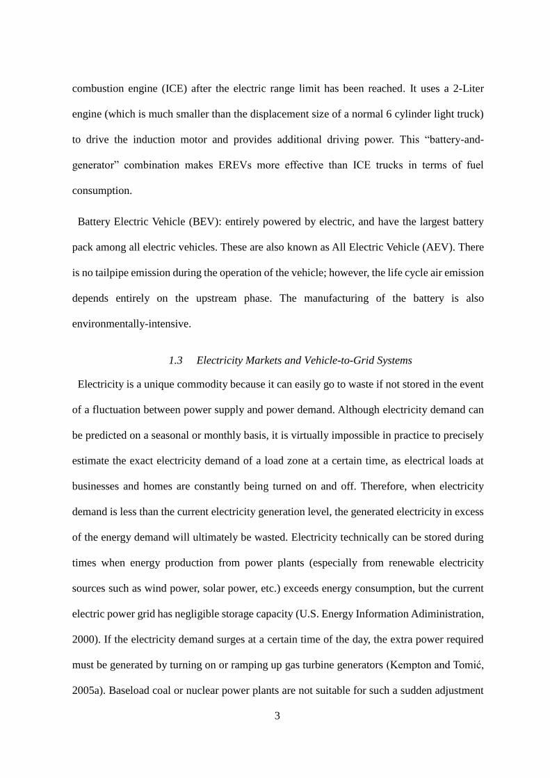
combustion engine (ICE) after the electric range limit has been reached. It uses a 2-Liter

engine (which is much smaller than the displacement size of a normal 6 cylinder light truck)

to drive the induction motor and provides additional driving power. This “battery-and-

generator” combination makes EREVs more effective than ICE trucks in terms of fuel

consumption.

Battery Electric Vehicle (BEV): entirely powered by electric, and have the largest battery

pack among all electric vehicles. These are also known as All Electric Vehicle (AEV). There

is no tailpipe emission during the operation of the vehicle; however, the life cycle air emission

depends entirely on the upstream phase. The manufacturing of the battery is also

environmentally-intensive.

1.3 Electricity Markets and Vehicle-to-Grid Systems

Electricity is a unique commodity because it can easily go to waste if not stored in the event

of a fluctuation between power supply and power demand. Although electricity demand can

be predicted on a seasonal or monthly basis, it is virtually impossible in practice to precisely

estimate the exact electricity demand of a load zone at a certain time, as electrical loads at

businesses and homes are constantly being turned on and off. Therefore, when electricity

demand is less than the current electricity generation level, the generated electricity in excess

of the energy demand will ultimately be wasted. Electricity technically can be stored during

times when energy production from power plants (especially from renewable electricity

sources such as wind power, solar power, etc.) exceeds energy consumption, but the current

electric power grid has negligible storage capacity (U.S. Energy Information Adiministration,

2000). If the electricity demand surges at a certain time of the day, the extra power required

must be generated by turning on or ramping up gas turbine generators (Kempton and Tomić,

2005a). Baseload coal or nuclear power plants are not suitable for such a sudden adjustment

4

requirement, and the frequent turning on and turning off of gas turbine generators leads to a

relatively low fuel efficiency.

From the grid operators’ perspective, the current electricity market provides four different

types of electricity services:

Baseload power, a.k.a. “bulk” power, is generated most commonly by large coal or nuclear

power plants on a round-the-clock basis. It has the lowest electricity unit cost, but the

generators commonly take days to start up or shut down, making it practically impossible

for them to respond to rapid system fluctuations.

Peak load power is typically generated by natural gas turbines when high electricity usage

is predicted, such as during summer afternoons. Peak power has higher prices in the

electricity market and, due to the peak power market’s relatively predictable demand

pattern, generators can be adjusted in advance to accommodate the additional demands.

In addition to generating baseload and peak power, the grid also needs ancillary services to

maintain grid reliability and stability. Two types of ancillary services are spinning reserves

and regulation services.

Spinning reserves mainly provide backup capacity to the grid and stabilize system

frequencies in the event of a generator failure or other such emergency.

Regulation services, namely Automatic Generation Control (AGC) services, serve as grid

stabilizers, maintaining system voltages and grid frequencies as needed, which is currently

accomplished by ramping up/down the output of the generator in question, in accordance

with an ISO’s regulation up/down signals.

Regulation services are mainly controlled by Independent System Operators (ISOs) and/or

Regional Transmission Organizations (RTOs). These entities are responsible for non-

5

discriminatory access to electricity transmission within a region, monitoring transmission,

and maintaining reliability of the grid. Although they do not own transmission, they help

coordinate transmission as well as plan for future transmission needs. They accomplish these

objectives through the use of energy, capacity and ancillary services markets. Due to rapid but

short demand periods and high electricity unit prices, the ancillary services market requires

flexible power supply methods and sources. studies have shown that electricity storage

methods such as batteries not only have extremely fast response times, but may also be two

to three times as effective as gas turbine generators for grid balancing purposes (Lin, 2011;

Makarov et al., 2012).

Currently in the U.S. there are several stationary battery facilities that provide grid stabilizing

services, with capacities ranging from 1 MW to 20 MW (Lin, 2011). These high-capacity

battery packs usually require an enormous capital investment and are thus far used only for

energy storage. However, if the existing U.S. light vehicle fleet were electrified, the resultant

total power capacity would be about 24 times more than that of the entire electricity generation

system (Kempton and Tomić, 2005b).

Vehicle-to-Grid technology utilizes the existing battery capacity of idle EVs as a means to

store electricity and then respond to grid operator request signals on a minute-by-minute basis,

making it a great ancillary service option. EV battery capacity is already routinely plugged

into the grid for charging, and has significant potential to serve as grid storage and capacity

to be used for grid stabilization services. Furthermore, with the introduction of government

incentives and reductions in manufacturing costs due to large-scale battery production, EVs

are expected to have greater market penetration levels over the next 15 years (Noori and Tatari,

2016). In fact, every major car manufacturer today has already manufactured one or more

electric vehicle models with significantly higher fuel economy levels than Internal

6

Combustion Engine Vehicles (ICEVs). Passenger cars are parked for most of the time in any

given day, and even during rush hours in California, only 10% of vehicles are on the road,

while the remaining 90% of vehicles are potentially available to the grid (Kempton et al.,

2001). For Plug-in Electric Vehicles (PHEVs) and Battery Electric Vehicles (BEVs), given

certain upgrades, existing systems are technologically capable of supporting the grid.

Therefore, with limited onboard meter and home wiring upgrades, EVs can be used as an ideal

grid electricity storage solution.

And from the service carriers’ perspective, alternative vehicle technologies, such as BEVs,

have the potential to minimize the negative environmental impacts of the transportation sector,

but there are several barriers to their widespread adoption, such as high initial cost; lack of a

public charging infrastructure network; apprehension about the limited range of EVs; and the

long charging times of EVs (Jones and Zoppo, 2014). One potential benefit that could drive

adoption in spite of these challenges, is the potential for an electrified vehicle fleet to generate

new revenue streams for the businesses and individuals who own alternative fuel vehicles

(Onat et al., 2014b). Modeling customer behavior is an important step towards identifying the

barriers to widespread adoption of BEVs and developing strategies to harness this technology

efficiently. BEVs can serve as a storage system for the electric power grid, termed V2G system,

and may create monetary saving opportunities, help widespread adoption of BEVs, and

minimize negative environmental impacts of both the energy and transportation sector. In this

study, the regional life cycle emissions savings and net revenue of V2G ancillary service

(regulation) are explored from a customer perspective.

The power provided by a single vehicle is little more than a noise to the grid (Guille and

Gross, 2009), but the combined power of 100 EVs with average power outputs of 15 kW each

amounts to approximately 1MW of grid support, which is a typical ancillary service minimum

7

contract amount (Kempton and Tomić, 2005b). The contract for such a V2G ancillary service

could be between vehicle drivers and utility companies and/or grid operators, and while V2G

services are being provided, each individual driver could preset the upper limit of the

electricity that he/she is willing to provide via the service, with the driver receiving

compensation and/or rewards for providing both the additional power capacity or capability

and the actual energy output.

1.4 Vehicle-to-Grid Systems and the Water-Energy Nexus

Electric power and transportation systems are the most important networks that connect all

the functional units in a city. A well-designed transportation system helps people whom are

the essential elements of the society to reach their destination or the necessities of life.

However, renewable energy sources such as wind or solar are intermittent. Hence a high level

of wind or solar power penetration requires a significant amount of ancillary services to

stabilize grid fluctuations. On the other hand, massive adoption of electric vehicles may also

cause marginal generation which mainly relies on non-renewable energy sources if the

charging behavior of electric vehicles are not regulated.

A system which further combines the electric power system and the public or private

transportation systems through vehicle-to-grid (V2G), vehicle-to-home (V2H), vehicle-to-

building (V2B) and vehicle-to-infrastructure (V2X) system helps integrate all the elements in

the gird. These elements include large-scale renewable energy, community-level renewable

energy, roof top solar panels, homes, commercial buildings and grid operators, and electric

vehicles. Electric vehicles will serve as mobile storage with great flexibility after a certain

BEV or HEV market penetration is reached.

Meanwhile, the supply of water and the generation of electric power are heavily

interconnected. To achieve an overall improvement in water preservation, GHG emission

8

mitigation and energy consumption reduction, the water-energy nexus must be addressed as a

whole. The current U.S. energy generation system relies mostly on coal or natural gas; yet

both the extraction of gas process and the operation of thermoelectric plants are water-

intensive. The majority of renewable energy sources consisting of biomass relies heavily on

water due to crop irrigation. On the other hand, the treatment and the transportation of water

consumes a significant amount of water. Furthermore, the structural stability of the water-

energy nexus will be challenged because of water demand increases due to residential and

agricultural expansion as well as energy consumption and GHG emission caused by

transportation.

There are three methods to improve the reliability of the nexus but there is no ultimate

solution without any tradeoff:

Improving the cooling system of thermoelectric power plants (Sovacool and Sovacool,

2009). Advanced power plants with closed-loop may reduce the water withdrawals but

may also increase water consumption. And the speed of efficiency improvement could

not catch up the growth of electricity demand.

Reducing peak demand in industrial and residential sector (Sovacool and Sovacool, 2009).

By doing so, the inefficient operation of combustion turbines could be mitigated.

However, such method requires cooperation from the industry and a well-established

smart grid system.

Deploying renewable energy. Florida has good solar and offshore wind power potential,

and these power sources have limited or zero carbon and water footprint. However, wind

and solar are intermittent, so to balance the fluctuations of different time intervals

ancillary services which rely on low-efficiency combustion turbine have to be purchased.

V2G technologies provide solutions to two of the aforementioned tradeoffs. It utilize the

9

battery capacity as grid storage methods which have been proven to be two to three times

more efficient than combustion turbines (Lin, 2011). With the help of bidirectional chargers,

the owner of the EV could plug their vehicle into the grid and provide power capacity services

to the grid operators in exchange for financial benefits. And with the extra storage capacity

online, significantly more wind and solar energy can be balanced and stored, making

renewable energy more cost-effective. Hence the entire electricity mix could be “cleaner” in

terms of energy and water consumption. Furthermore, as the smart grid being implemented,

residential or commercial electricity users can choose to avoid the electricity usage peak or

even supply a certain amount of energy back to the grid through their EVs or battery units so

that the peak of the grid could be “shaved”.

1.5 Problem Statement and Research Objectives

To fully understand the feasibility and potential outcomes of integrating EVs into the water-

energy nexus, the following questions should be investigated:

1. Although hybrid or battery electric vehicles can effectively reduce tailpipe emissions, will

the life cycle environmental impact be reduced given various electric power source percentage?

And what’s the impact comparison between EVs and other alternative technologies?

2. With the consideration of energy loss and battery pack replacement, will the

implementation of V2G systems mitigate the overall GHG emissions and create revenue for

EV owners?

3. Will there be any form of air emission impact if large amount of electric vehicles being

adopted in a short amount of time? Will the unregulated charging of EVs generate significant

amount of emissions?

4. Taking the spatial electricity market variance and future clean energy integration plan into

10

account, will V2G systems provide sufficient storage capacity to the grid and facilitate the

integration of more clean energy?

5. What is the role of future V2G systems in the water-energy nexus, what are the interactions

between V2G systems and other social and economic aspects, and will it facilitate the

optimization of the current energy structure with the consideration of its economic and social

impacts?

6. What are the other underlying relationships that may affect the transportation-energy-

water network? Taking the uncertainties into consideration, will the V2G system as a

connection between the transportation and energy systems have positive influences?

To answer these questions, a series of studies from an individual vehicle level to a water-

energy system level are conducted in this dissertation. In Chapter 2, the alternative fuel

options of medium-duty trucks in commercial delivery fleets, which are most likely the first

carriers of V2G technologies, are analyzed; and their life cycle environmental impacts are

evaluated in different regions of the U.S. In Chapter 3, the operation mechanism of V2G

technologies in association with the charging and discharging of electric vehicles are

researched; and the life cycle greenhouse gas emissions of this system are calculated based

on various grid fluctuation and vehicle battery degradation scenarios to assess the feasibility

of the V2G system. In Chapter 4, the spatial and temporal variance and system uncertainties

of the feasible Vehicle-to-Grid system is further studied; the projection of the future emission

mitigation is also included in this phase. In Chapter 5, based on the assumption that V2G

systems are utilized to provide ancillary service for newly integrated wind power, the

comparison of greenhouse gas emission mitigation of the V2G systems and the additional

emissions caused by electric vehicle marginal charging is studied. In Chapter 6, the research

scope is further expanded to explore the impact of V2G systems in the water-energy nexus,

11

and the environmental, economic and social networks are simulated through system dynamic

modeling. As a further development of Chapter 5, the system dynamics model is consolidated,

and incorporated with an uncertainty analysis to predict the impacts of the V2G system to the

future transportation-energy-water network.

The six research objectives from Chapter 2 to Chapter 7 expands from one vehicle to a multi-

system nexus with the consideration of social, environmental and economic factors. Figure 1

depicts the flow of study and methodologies of each research phase.

Figure 1 Hierarchical relationships and methodologies of the research objectives

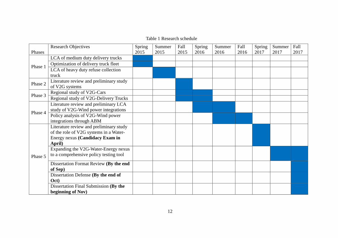
The schedule of study including the tasks in each phase are shown in Table 1.

12

Table 1 Research schedule

Phases

Research Objectives Spring

2015

Summer

2015

Fall

2015

Spring

2016

Summer

2016

Fall

2016

Spring

2017

Summer

2017

Fall

2017

Phase 1

LCA of medium duty delivery trucks

Optimization of delivery truck fleet

LCA of heavy duty refuse collection

truck

Phase 2 Literature review and preliminary study

of V2G systems

Phase 3 Regional study of V2G-Cars

Regional study of V2G-Delivery Trucks

Phase 4

Literature review and preliminary LCA

study of V2G-Wind power integrations

Policy analysis of V2G-Wind power

integrations through ABM

Phase 5

Literature review and preliminary study

of the role of V2G systems in a Water-

Energy nexus (Candidacy Exam in

April)

Expanding the V2G-Water-Energy nexus

to a comprehensive policy testing tool

Dissertation Format Review (By the end

of Sep)

Dissertation Defense (By the end of

Oct)

Dissertation Final Submission (By the

beginning of Nov)

13

2 HYBRID MULTI-REGIONAL INPUT-OUTPUT LIFE CYCLE

ASSESSMENT OF ELECTRIC DELIVERY TRUCKS

A partial work of this chapter has been published in the Journal of Transportation Research

Part D: Transport and Environment with the title of “Carbon and energy footprints of electric

delivery trucks: A hybrid multi-regional input-output life cycle assessment” (Zhao et al.,

2016b)

Due to frequent stop-and-go operation and long idling periods when driving in congested

urban areas, the electrification of commercial delivery trucks has become an interesting topic

nationwide. In this study, environmental impacts of various alternative delivery trucks

including battery electric, diesel, diesel-electric hybrid, and compressed natural gas trucks are

analyzed. A novel life cycle assessment method, an environmentally-extended multi-region

input-output analysis, is utilized to calculate energy and carbon footprints throughout the

supply chain of alternative delivery trucks. The uncertainties due to fuel consumption or other

key parameter variations in real life, data ranges are taken into consideration using a Monte

Carlo simulation. Furthermore, variations in regional electricity mix greenhouse gas emission

are also considered to present a region-specific assessment for each vehicle type. According

to the analysis results, although the battery electric delivery trucks have zero tailpipe emission,

electric trucks are not expected to have lower environmental impacts compared to other

alternatives. On average, the electric trucks have slightly more greenhouse emissions and

energy consumption than those of other trucks. The regional analysis also indicates that the

percentage of cleaner power sources in the electricity mix plays an important role in the life

cycle greenhouse gas emission impacts of electric trucks.

14

2.1 Electric Delivery Truck Introduction and Literature Review

By the year 2015, there were 260 million registered vehicles in the US, more than 20% of

which are pickup trucks or step vans (Hedges & Company, 2015), and the average fuel

economy of these trucks is 10 mile per gallon (MPG). The low fuel economy is because these

Class 3 to Class 6 trucks operate on lower speed urban roads in stop-and-go traffic and have

significantly longer idling times than trucks of other sizes. Consequently, 21.1%-34.1% of the

total fuel consumption was used during non-productive moments because of the relatively

long idling time (Gaines et al., 2006). A study from the National Academy of Sciences showed

that the Fuel Consumption Reduction Potential of a “class 6 box truck” is 47% (National

Research Council, 2010). And with the great potential of fuel saving, the National Highway

Traffic Safety Administration (NHTSA) set a standard for diverse truck fleets to reduce fuel

consumption and GHG emissions from delivery trucks by 10% by model year 2018 (The

White House, 2014). Therefore, due to their operation feature and environmental impact

reduction potential, medium duty urban commercial (parcel) delivery trucks are considered

as suitable applications for alternative fuel types.

In addition to conventional diesel delivery trucks, trucks using alternative fuels can also be

utilized to reduce environmental impacts; given the long idling time and frequent stop-and-

go driving patterns, a diesel electric hybrid vehicle might be a good solution because of its

braking regeneration feature. The National Renewable Energy Laboratory (NREL) has

conducted a 36-month evaluation of United Parcel Service (UPS) Diesel hybrid-electric

delivery vans (Lammert and Walkowicz, 2012). Compressed natural gas (CNG) vehicles also

have their own advantages, such as limited cost of conversion from existing diesel-powered

trucks and low CNG fuel prices The CNG delivery trucks have been tested in the NREL truck

evaluation project (Chandler et al., 2002). Finally, the most widely discussed and tested

vehicle type is the plug-in all-electric vehicle. Companies like FedEx, Staples, and Frito Lay

15

all have cooperated with NREL and evaluated pure electric vehicles like Navistar (National

Renewable Energy Laboratory, 2014a) and Smith Newton since 2009 (National Renewable

Energy Laboratory, 2014b). The electrification of delivery trucks has unique advantages, first,

that truck drivers do not have “range anxiety” as personal electric car drivers because of the

fixed driving routine, and second, that a large fleet size of electric vehicles makes centralized

charging stations available, reducing overall charging cost through charging schedule

optimization or vehicle-to-grid (V2G) services.

Regarding commercial delivery trucks, research has been conducted focusing on

comprehensive analyses of life cycle ownership cost minimization, electric vehicle range,

fleet size, and energy consumption (Davis and Figliozzi, 2013). There is also a study available

about fleet replacement strategies based on the purchase prices and maintenance costs of

Lithium battery trucks and conventional trucks (Feng and Figliozzi, 2013). A Life Cycle

Assessment (LCA) of batteries and diesel trucks has also been studied with respect to energy,

GHG emissions, and cost effectiveness (Lee et al., 2013a). However, there is no study

available in current literature that involves a comparative input-output LCA among diesel,

hybrid, CNG, and battery electric delivery trucks. Furthermore, previous studies are

conducted mainly based on a 2002 EIO-LCA model, which may not be able to reflect the

environmental impacts of current industrial sectors. In this regard, This study is conducted

based on an environmentally-extended multi-region hybrid LCA, and the life-cycle (both

upstream/indirect and downstream/direct) environmental impacts of conventional diesel

trucks, diesel-electric hybrid trucks, CNG trucks, and two types of plug in electric trucks are

evaluated to provide answers and insights to the following questions:

Considering all life cycle phases and the entire supply chain, which has a better

environmental performance: a conventional truck, or an alternative-fuel truck?

16

Considering how the electricity generation mix makes a significant difference with

respect to GHG emissions from region to region, which regions are more suitable for

replacing conventional trucks with electric trucks?

Which alternative-fuel truck has a higher GHG emission reduction and energy saving

potential?

2.2 Method

2.2.1 Life cycle assessment

Life Cycle Assessment (LCA) is an established but still evolving technique designed to assess

environmental impacts and resource consumption associated with all stages of a product’s life

cycle from raw material extraction to end-of-life disposal or recycling (Finnveden et al., 2009;

Onat et al., 2014a, b). By compiling an inventory of relevant material/energy inputs and

environmental releases, LCA can help us to assess a product’s life cycle environmental impact

by evaluating the potential impact associated with the identified input and output. There are

three main LCA methods: Process-based LCA, Input-Output LCA, and Hybrid LCA. Process-

based LCA was initially created to capture the life cycle impact of a product from “cradle to

grave”, but its “holistic” nature is both process based LCA’s strength and limitation (Guinée,

2001). Some part of the system has to be cut off or neglected because even the simplest product

is produced by an extremely complicated upstream system (Mattila et al., 2010). Input-Output

LCA, on the other hand, was used to analyze impacts by categorizing products or services with

respect to local industry sectors. Input-Output LCA is able to reflect emissions from the entire

supply chain, avoid truncation error, and provide a holistic analysis (Kucukvar et al., 2014a;

Kucukvar and Tatari, 2013). However, because of the aggregation of the Input-Output LCA

17

approach, some products or processes with diversity have to be allocated to the same sector.

Also, the Input-Output approach can provide information for only typical processes that are

well represented by Input-Output categorizes, while all other processes can be modeled via the

process-based method (Suh et al., 2004). For example, in this study, the processes of burning

fuel are not incorporated in the Input-Output method, and so we need to hybridize the model

by including process-based LCA (P-LCA). The Input-Output based LCA models provide a top-

down analysis using sectorial monetary transaction matrixes considering complex interactions

between the sectors of a single country. Although single-region Input-Output models have been

widely used in previous LCA studies for electric vehicles (Onat et al., 2015a; Onat et al., 2015b;

Onat et al., 2016b; Onat et al., 2015c), Multi Region Input-Output (MRIO) models represent

the state-of-the-art in the estimation of environmental footprint of production at global scale

(Feng et al., 2011; Kucukvar et al., 2016; Kucukvar and Samadi, 2015). In a MRIO framework,

these flows present the value of imports and exports per country and economic sector. All

imports and exports are then merged into one consistent financial accounting framework. This

combined inter-industry transaction matrix is linked to primary inputs between economic

sectors and final demand categories including household consumption, private fixed

investments, and government purchases and investments (Wiedmann, 2009; Wiedmann et al.,

2011). Among the MRIO initiatives, the Externality Data and Input-Output Tools for Policy

Analysis (EXIOPOL) is one of the most developed MRIO initiatives distinguishing 163

industry sectors and products, and supported by the European Commission under the 6th

framework programme for research. This project aims to advance global symmetric MRIO

tables for 43 countries including 27 EU member states and 16 other major countries (95% of

world economy). The EXIOPOL database includes several environmental and socioeconomic

indicators such as global warming potential, total material requirement, land use, water use,

employment, external costs, etc. In this paper, a standard MRIO analysis that is extended with

18

greenhouse gas emissions and energy use data is developed. Using the EXIOPOL database, the

environmentally-extended multi-region hybrid LCA (EE-MR-HLCA) model that integrate the

advantages of both Process-based LCA and EE-MR-HLCA approaches is developed, and these

different types of hybrid LCA approaches are well illustrated in literature (Bilec et al., 2006).

The hybrid LCA used in this study follows these procedures: First the scope of the life cycle

phase of each type of vehicle is defined, and then the cost of each phase is identified and

calculated. Life cycle cost data is then used as input data and plugged into an EE-MR-HLCA

model (Exiobase 2, 2015). The output was derived in terms of environmental indicators.

2.2.2 Scope of analysis

Figure 2 depicts the flow chart of different life cycle phases utilized for the LCA study, as

well as the system scope, which includes the vehicle and battery manufacturing phases, the

maintenance/repair phase, the fuel and infrastructure production phases, and the vehicle

operation phase. There is no available data for the delivery truck recycling percentage as well

as a unified technology of recycling/reusing the vehicle body components or the battery, hence,

the end-of-life (EOL) phases of the vehicle and battery are not included in this study. The GHG

emissions and energy consumption of vehicle manufacturing, fuel (including diesel, CNG and

electricity) production phase, vehicle maintenance phase and charging/refueling infrastructure

are evaluated by a 2007 regional EE-MR-HLCA model (Exiobase 2, 2015). However, the

manufacturing of high capacity lithium ion battery is environmental intense and cannot be

represented by the “primary battery manufacturing” sector in the EE-MR-HLCA model. And

as mentioned in Section 2.1, the tailpipe environmental impact is not included by the EE-MR-

HLCA model. Therefore, the GHG emission and energy consumption of the vehicle battery

manufacturing phase and tailpipe phase are analyzed by process-based LCA, these two phases

are further discussed in Section 2.4.1 and Section 2.4.2. The direct and indirect impacts of these

19

phases are evaluated based on 150,000 (15,000 per year) Vehicle Miles of Travel (VMT) for

each type of vehicle, the functional unit being the lifetime VMT of the truck.

Figure 2 System boundaries

2.2.3 Vehicle characteristics

Table 1 shows the basic features and characteristics of the researched vehicles. The UPS 2006

P70D diesel step van with a freightliner chassis is used as a reference object. It is a class 4

delivery truck with a curb weight of 9,450 lb., a payload of 7,250 lb., and an average diesel

fuel efficiency of approximately 10 miles per gallon (Lammert and Walkowicz, 2012). These

specific types of diesel truck, as well as other trucks with similar chassis, body and payload

design, have been widely used by shipment and logistics departments and companies like UPS

and FedEx. Other vehicles of different fuel types were incorporated in the assessment for

comparison to conventional diesel delivery trucks. The diesel-electric hybrid truck Freightliner

P70D, which has braking regeneration function but a slightly lower Gross Vehicle Weight

(GVW), had been tested by the National Renewable Energy Laboratory (NREL) as an

20

alternative-fuel truck option (Lammert and Walkowicz, 2012). It should be noted that this

hybrid truck is powered by diesel and has no grid accessibility; hence its battery capacity is

fairly small. Since CNG trucks are commonly modified from diesel trucks, they are assumed

to have the similar feature as diesel trucks except for the additional natural gas storage tank

weight, therefore, the truck curb weight increases to 10,710 lb. and the payload of the truck

reduces to approximately 6,000 lb. (Argonne National Laboratory, 2016). The average fuel

efficiency of CNG trucks is shown as diesel equivalent in Table 1. For battery electric trucks

which are powered purely by the electricity stored in the battery, the class 3 Navistar E-star (E-

3) and class 5 Smith Newton (E-5) battery electric delivery trucks are evaluated in this study.

The curb weight, payload and fuel efficiency of the two types of electric trucks are concluded

from multiple testing results including the evaluations from NREL (Chambers, 2010; National

Renewable Energy Laboratory, 2014a, b; Vlack, 2013). These two battery electric trucks are

powered by high-capacity lithium ion battery packs which produce significant environmental

impacts during manufacturing, the battery-related impacts are further discussed in the

following section.

21

Table 2 Basic vehicle characteristics

Fuel Type Diesel

Diesel

Electric

Hybrid

CNG

Class 3

Battery

Electric

Class 5

Battery

Electric

Weight Class 4 or 5 3 or 4 4 3 5

Curb Weight

(lb.)

9,450 9,450 10,710 7,700 9,700

Payload (lb.) 7,250 7,000 5,990 4,000 12,324

Average Fuel

Economy

10.73

MPG

13.01 MPG 8.62 (MPG

Equivalent)

0.91

(KWh/mile)

1.93

(KWh/mile)

Battery

Capacity

(KWh)

- 1.80 - 80 100

Battery Weight

(lb.)

- - - 1,357 1,696

* Truck Make, Model and Year: Diesel (Freightliner P700 UPS Delivery Truck, year 2006), hybrid

(Freightliner P70H UPS Low Emission Hybrid Delivery Truck, year 2007), CNG (Grumman Olson UPS

CNG Truck, year 1997), E-3 (Navistar E-Star FedEx Class 3 Step Van, year 2010), E-5 (Smith Newton Class

5 Truck, year 2006)

2.3 Life cycle inventory, parameters and assumptions

For all of the trucks researched, each truck’s components and life cycle phases are divided

into the manufacturing phases, the operation phase, and the charging infrastructure phase as

categorized by the sectors of Environmentally Extended Supply and Use/Input Output

Database (Exiobase 2, 2015), which are summarized in Table 3. Due to the model year

variation of the researched trucks, some of the data is from different years, so the year 2007

was set as the base year and all life cycle monetary value are converted to 2007 US dollars,

using the Producer Price Index (PPI) for comparability.

As shown by Table 3, the GHG emissions and energy consumptions of electricity generation,

transmission and distribution vary based on the electricity power source. In 2015, 33% of the

U.S. electricity generation comes from coal, 33% from natural gas, 20% from nuclear, 6%

from hydropower, 1% from petroleum and 7% from renewable energy which consists 1.6%

biomass, 0.4% geothermal, 0.6% solar and 4.7% wind power (U.S. Environmental Protection

22

Agency, 2015c). And the reginal electricity mix varies significantly, some areas rely heavily

on coal as energy source (such as Midwestern regions) while some areas have adopted large

amount of clean energy (California or northeastern regions). Therefore, two analyses are

conducted in this research, the first national analysis is performed based on national electricity

mix, and the second analysis is a regional environmental impact comparison that reflects how

the electricity mix affects the environmental performance of different types of delivery trucks.

As noted before, electric truck battery manufacturing and vehicle tailpipe emissions/energy

consumption are not included in the EE-MR-HLCA inventory; they are calculated separately

through process-based LCA.

23

Table 3 Exiobase EE-MR-HLCA multipliers

Life Cycle Phases Exiobase Sector

CO2

(metric

ton/ per

million $)

CH4 (metric

ton/ per

million $)

CH4-CO2

Equivalent

(metric ton/ per

million $)

N2O

(metric

ton/ per

million $)

N2O CO2

Equivalent

(metric ton/

per million $)

Energy

(TJ/per

million $)

Electricity

Generation,

Transmission and

Distribution

Production of electricity by coal 24,476.12 0.26 6.56 0.39 117.25 290.82

Production of electricity by gas 12,014.79 0.22 5.57 0.04 12.11 216.71

Production of electricity by nuclear 60.71 0.00 0.09 0.00 1.31 320.55

Production of electricity by hydro 74.79 0.00 0.10 0.01 1.55 9.70

Production of electricity by wind 76.91 0.00 0.11 0.01 1.60 6.75

Production of electricity by petroleum 20,266.89 0.75 18.75 0.99 293.67 289.52

Production of electricity by biomass and

waste

7,721.27 9.15 228.67 1.23 365.07 351.65

Production of electricity by solar

photovoltaic

87.87 0.00 0.12 0.01 1.78 6.88

Production of electricity by Geothermal 82.82 0.00 0.11 0.01 1.70 6.63

Transmission of electricity 125.96 0.01 0.20 0.01 2.83 5.00

Distribution and trade of electricity 110.16 0.01 0.18 0.01 2.68 3.33

Vehicle

Manufacturing

Manufacturing of motor vehicles, trailers

and semi-trailers

488.01 0.02 0.48 0.02 6.93 11.98

CNG Production

Extraction of natural gas and services

related to natural gas extraction,

excluding surveying

1,044.53 0.03 0.73 0.03 8.04 21.05

Vehicle Maintenance

and Repair

Maintenance, repair of motor vehicles,

motor vehicles parts

187.86 0.01 0.21 0.01 3.81 5.19

Diesel Production

Extraction of crude petroleum and

services related to crude oil extraction,

excluding surveying

312.41 0.01 0.34 0.02 5.30 8.27

Charging

Infrastructure

Manufacture of electric machinery and

apparatus

336.71 0.97 24.20 0.01 3.69 5.76

Refueling

Infrastructure

Manufacture of machinery 509.26 1.42 35.41 0.02 5.16 8.43

24

Table 4 includes the data sources and the assumptions regarding the parameters. The vehicle

retail prices are obtained from multiple sources. The price of each vehicle type varies within

a certain range, so the retail price is assumed to follow a uniform distribution. The

corresponding minimum and maximum value are listed in Table 4. There is no available price

data for the CNG truck, however, CNG trucks are often modified from regular trucks and the

modification cost is approximately $20,000 for a medium duty delivery truck (Argonne

National Laboratory, 2016). Also, because of the CNG truck tested in the literature is a fairly

earlier model, it may not reflect the fuel economy of current CNG trucks, to tackle this issue,

in addition to the fuel economy data set obtained from the 2002 CNG truck testing report

(Chandler et al., 2002), an additional group of data concluded by multiplying the diesel truck

fuel economy by 0.9 has also been added to the CNG truck fuel economy distribution

calculation. The reason is that the fuel economy (diesel equivalent) of a medium duty CNG

truck is approximately 90% of the fuel economy of a regular diesel truck (Argonne National

Laboratory, 2015) due to the weight of the additional compressed natural gas tank. It should

be noted here that the high capacity battery pack accounts for a fairly large portion of the

vehicle price; hence the battery price is excluded from the battery electric vehicle retail price.

The environmental impact of battery manufacturing is evaluated by process-based LCA. The

maintenance costs are concluded from the tests conducted by NREL in different years, so they

are converted to 2007 price through PPI. Based on the testing results, it is assumed that the

fuel economy of the trucks follows a normal distribution. The mean and standard deviation

are shown in Table 4 as well. With the data provided in Table 4, the purchasing cost, life cycle

maintenance cost, battery cost and fuel cost of the researched trucks are prepared for the EE-

MR-HLCA calculation

25

Table 4 Vehicle data source

Parameters Unit Data Data Source

Diesel

Truck

Vehicle retail

price

$ Min: 42,864

Max: 65,000

(Argonne National Laboratory,

2016; Lammert and Walkowicz,

2012)

Maintenance cost $/mile 0.13 (Lammert and Walkowicz, 2012)

Fuel economy mile/gallon Mean: 10.73

StD: 1.067

(Lammert and Walkowicz, 2012)

Hybrid

Truck

Vehicle retail

price

$ Min: 60,000

Max: 105,000


2016; Lammert and Walkowicz,

2012)

Maintenance cost $/mile 0.141 (Lammert and Walkowicz, 2012)

Fuel economy mile/gallon Mean: 13.01

StD: 0.577

(Lammert and Walkowicz, 2012)

CNG Truck Vehicle retail

price

$ Min: 62,864

Max: 105,000


2016)

Maintenance cost $/mile 0.0684 (Chandler et al., 2002)

Fuel economy mile/gallon

(diesel

equivalent)

Mean: 8.62

StD: 0.974

(Chandler et al., 2002; Lammert

and Walkowicz, 2012)

Class 3

Battery

Electric

Truck

Vehicle retail

price

$ Min: 87,000

Max: 117,000


2016; Gallo and Tomic, 2013)

Battery capacity KWh 80 (National Renewable Energy

Laboratory, 2014a)

Maintenance cost $/mile 0.072 (Gallo and Tomic, 2013)

Fuel economy KWh/mile Mean: 0.91

StD: 0.09

(National Renewable Energy

Laboratory, 2014a)

Class 5

Battery

Electric

Truck

Vehicle retail

price

$ Min: 30,000

Max: 65,000

(Kurczewski, 2011)

Battery capacity KWh 100 (National Renewable Energy

Laboratory, 2014b)

Maintenance cost $/mile 0.0975 (Gallo and Tomic, 2013)

Fuel economy KWh/mile Mean: 1.93

StD: 0.259


Laboratory, 2014b)

Other

Parameters

Producer Price

Index (PPI)

- PPI Index

from 2001 to

2014

(U.S. Bureau of Labor Statistics,

2001, 2007, 2009, 2013, 2014)

Specific energy KWh/kg 0.13 (Argonne National Laboratory,

2016)

Diesel price $/gallon 2.40 (federal

and state tax

excluded)

(U.S. Energy Information

Adiministration, 2016b)

Electricity price cent/KWh 9.65 (U.S. Energy Information

Adiministration, 2014)

CNG price $/thousand

cf

8.5 (U.S. Energy Information

Adiministration, 2012)

CNG-diesel

conversion

cf/gallon

diesel

134.65 Converted by heat content

Battery price $/KWh 600 (Gallo and Tomic, 2013)

26

2.3.1 Manufacturing phase

The retail price of each vehicle is converted to the producer price by a retail-manufacturing

rate. For diesel, hybrid and CNG trucks, this rate is assumed to be 0.8 (Samaras and

Meisterling, 2008). Nevertheless, the retail-manufacturing rate of electric vehicles are

assumed to be 0.7 (Rogozhin et al., 2009) because of the higher profit potential. Also, as

mentioned before, the main difference between electric vehicles evaluation and non-electric

vehicles evaluation is the battery manufacturing phase of the former, so the manufacturing

phase consists of both non-battery automobile manufacturing and high-capacity battery

making, the latter of which is evaluated by process-based LCA. The process-based LCA data

is obtained from the GREET (Argonne National Laboratory, 2015) model, where GHG

emissions and energy consumption is assumed to be proportional to the battery

capacity/weight. And according to this model, the battery specific energy is assumed to follow

a uniform distribution of which the minimum value is 0.106 KWh/kg and the maximum value

is 0.133 KWh/kg. The literature indicates that ideally, the battery of an electric truck is

supposed to be replaced every 150,000 mile (Electrification Coalition, 2010), however, due

to the intensity of the operation, fast charging might be required and hence the battery life is

shortened. Therefore, it is assumed that two batteries are needed during the 150,000-mile

vehicle life time.

2.3.2 Operation Phase

The operation phase can be divided into two main sectors: the automobile maintenance and

repair sector, and the fuel sector. The latter, more specifically, includes diesel production,

electric power generation, transmission, and distribution, and natural gas distribution.

Furthermore, the fuel sector includes direct and indirect impacts. The indirect impact, also

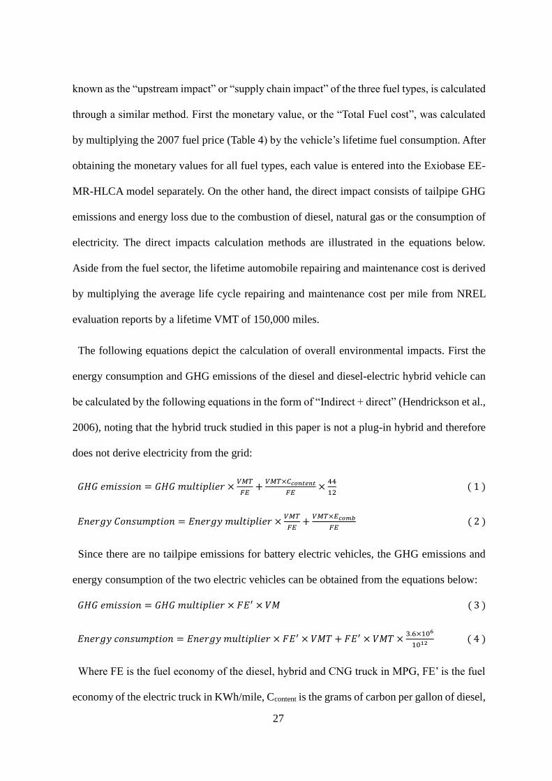
27

known as the “upstream impact” or “supply chain impact” of the three fuel types, is calculated

through a similar method. First the monetary value, or the “Total Fuel cost”, was calculated

by multiplying the 2007 fuel price (Table 4) by the vehicle’s lifetime fuel consumption. After

obtaining the monetary values for all fuel types, each value is entered into the Exiobase EE-

MR-HLCA model separately. On the other hand, the direct impact consists of tailpipe GHG

emissions and energy loss due to the combustion of diesel, natural gas or the consumption of

electricity. The direct impacts calculation methods are illustrated in the equations below.

Aside from the fuel sector, the lifetime automobile repairing and maintenance cost is derived

by multiplying the average life cycle repairing and maintenance cost per mile from NREL

evaluation reports by a lifetime VMT of 150,000 miles.

The following equations depict the calculation of overall environmental impacts. First the

energy consumption and GHG emissions of the diesel and diesel-electric hybrid vehicle can

be calculated by the following equations in the form of “Indirect + direct” (Hendrickson et al.,

2006), noting that the hybrid truck studied in this paper is not a plug-in hybrid and therefore

does not derive electricity from the grid:

𝐺𝐻𝐺 𝑒𝑚𝑖𝑠𝑠𝑖𝑜𝑛 = 𝐺𝐻𝐺 𝑚𝑢𝑙𝑡𝑖𝑝𝑙𝑖𝑒𝑟 ×𝑉𝑀𝑇

𝐹𝐸+

𝑉𝑀𝑇×𝐶𝑐𝑜𝑛𝑡𝑒𝑛𝑡

𝐹𝐸×

44

12 ( 1 )

𝐸𝑛𝑒𝑟𝑔𝑦 𝐶𝑜𝑛𝑠𝑢𝑚𝑝𝑡𝑖𝑜𝑛 = 𝐸𝑛𝑒𝑟𝑔𝑦 𝑚𝑢𝑙𝑡𝑖𝑝𝑙𝑖𝑒𝑟 ×𝑉𝑀𝑇

𝐹𝐸+

𝑉𝑀𝑇×𝐸𝑐𝑜𝑚𝑏

𝐹𝐸 ( 2 )

Since there are no tailpipe emissions for battery electric vehicles, the GHG emissions and

energy consumption of the two electric vehicles can be obtained from the equations below:

𝐺𝐻𝐺 𝑒𝑚𝑖𝑠𝑠𝑖𝑜𝑛 = 𝐺𝐻𝐺 𝑚𝑢𝑙𝑡𝑖𝑝𝑙𝑖𝑒𝑟 × 𝐹𝐸′ × 𝑉𝑀 ( 3 )

𝐸𝑛𝑒𝑟𝑔𝑦 𝑐𝑜𝑛𝑠𝑢𝑚𝑝𝑡𝑖𝑜𝑛 = 𝐸𝑛𝑒𝑟𝑔𝑦 𝑚𝑢𝑙𝑡𝑖𝑝𝑙𝑖𝑒𝑟 × 𝐹𝐸′ × 𝑉𝑀𝑇 + 𝐹𝐸′ × 𝑉𝑀𝑇 ×3.6×106

1012 ( 4 )

Where FE is the fuel economy of the diesel, hybrid and CNG truck in MPG, FE’ is the fuel

economy of the electric truck in KWh/mile, Ccontent is the grams of carbon per gallon of diesel,

28

and Ecmb is the energy content of diesel fuel (Hendrickson et al., 2006). One gallon diesel

contains 128,700 btu energy and 1 btu equals to 1,055J. EE-MR-HLCA multipliers are derived

from the Exiobase model, VMT is assumed to be 150,000 miles, and the parameters of the

vehicles are as shown in Table 3 and 4. For the CNG truck, the GHG emission and energy

consumption calculation follows Equation (1) and (2) but the Ccontent and Ecmb are replaced by

the carbon and energy content of natural gas.

2.3.3 Charging and refueling infrastructure

The charging equipment (level 2) cost of battery electric vehicles is assumed to be $7,500

(Gallo and Tomic, 2013), and is categorized as “Miscellaneous electrical equipment

manufacturing”. And it is assumed that each electric truck requires one charging device.

It is assumed that the diesel and hybrid trucks are refueled by existing gas stations, but the

operation of a CNG commercial delivery truck fleet requires a new CNG refueling station,

which mainly consists of a gas compressor and electronic devices. A typical parcel delivery

truck fleet has 20 to 30 trucks, and the CNG refueling station for a truck fleet of such size

costs approximately $20,000 ($13,000 for the compressor and $7,000 for the electronic

devices) (Gonzales, 2014). And the total cost of the refueling station is distributed to the 30

CNG trucks in the fleet.

2.4 Results

Analysis results are presented in the following subsections based on the environmental

impacts of alternative commercial trucks and the comparison of regional GHG emission from

each of these trucks. In order to simulate a practical situation and to take uncertainties into

consideration, a Monte Carlo Simulation (MCS) method is used in the calculation.

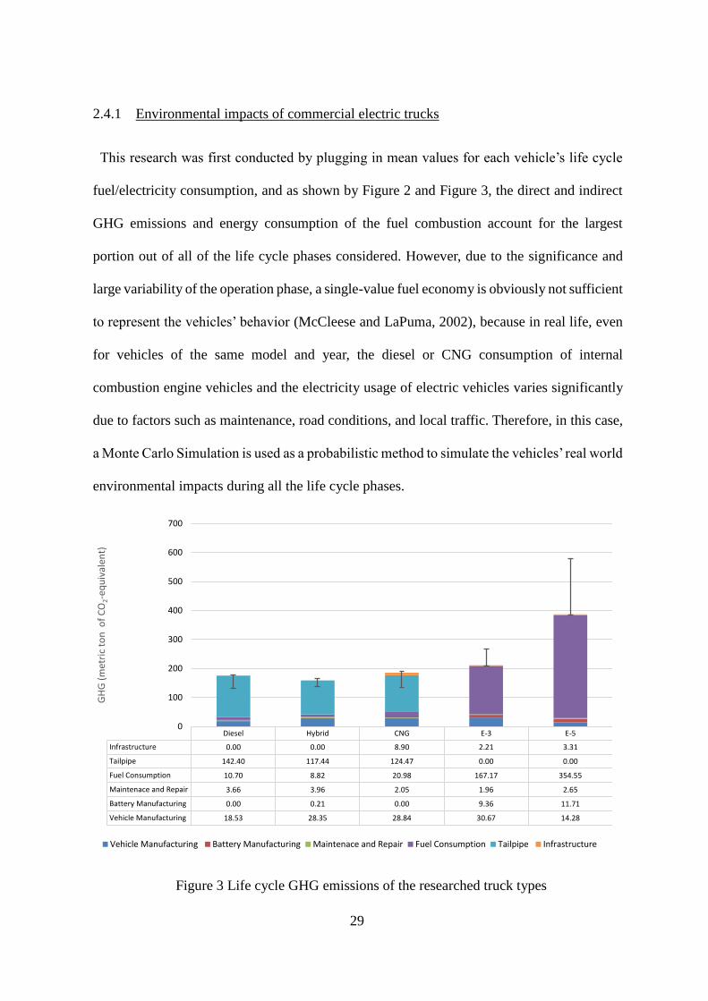
29

2.4.1 Environmental impacts of commercial electric trucks

This research was first conducted by plugging in mean values for each vehicle’s life cycle

fuel/electricity consumption, and as shown by Figure 2 and Figure 3, the direct and indirect

GHG emissions and energy consumption of the fuel combustion account for the largest

portion out of all of the life cycle phases considered. However, due to the significance and

large variability of the operation phase, a single-value fuel economy is obviously not sufficient

to represent the vehicles’ behavior (McCleese and LaPuma, 2002), because in real life, even

for vehicles of the same model and year, the diesel or CNG consumption of internal

combustion engine vehicles and the electricity usage of electric vehicles varies significantly

due to factors such as maintenance, road conditions, and local traffic. Therefore, in this case,

a Monte Carlo Simulation is used as a probabilistic method to simulate the vehicles’ real world

environmental impacts during all the life cycle phases.

Figure 3 Life cycle GHG emissions of the researched truck types

Diesel Hybrid CNG E-3 E-5

Infrastructure 0.00 0.00 8.90 2.21 3.31

Tailpipe 142.40 117.44 124.47 0.00 0.00

Fuel Consumption 10.70 8.82 20.98 167.17 354.55

Maintenace and Repair 3.66 3.96 2.05 1.96 2.65

Battery Manufacturing 0.00 0.21 0.00 9.36 11.71

Vehicle Manufacturing 18.53 28.35 28.84 30.67 14.28

0

100

200

300

400

500

600

700

GH

G (

met

ric

ton

of

CO

2-eq

uiv

alen

t)

Vehicle Manufacturing Battery Manufacturing Maintenace and Repair Fuel Consumption Tailpipe Infrastructure

30

Figure 4 Life cycle energy consumption of the researched truck types

NREL’s testing reports included fuel economy data for 11 diesel and hybrid delivery trucks

(Lammert and Walkowicz, 2012) and for 12 CNG delivery trucks (Chandler et al., 2002), as

well as seven quarters’ research for Navistar E-star from July 2012 to June 2014 (National

Renewable Energy Laboratory, 2014a) and 11 quarters’ research for Smith Newton from

November 2011 to June 2014 (National Renewable Energy Laboratory, 2014b). Based on the

observation of these data sets, they are assumed to follow a normal distribution, so the mean

values and standard deviations are calculated, and used as variables in the Monte Carlo

Simulation.

Figure 2 depicts the GHG emission impacts throughout the life cycle phases of all the truck

types. Based on the national average electricity mix, although there is no tailpipe emission

during the operation phase, battery electric trucks generate more GHG emissions than other

trucks from a life cycle perspective. For the electric delivery trucks, the majority of emissions

Diesel Hybrid CNG E-3 E-5

Infrastructure 0.000 0.000 0.138 0.035 0.052

Tailpipe 1.898 1.565 2.534 0.491 1.042

Fuel Consumption 0.278 0.229 0.419 3.285 6.968

Maintenace and Repair 0.099 0.107 0.056 0.053 0.072

Battery Manufacturing 0.000 0.000 0.000 0.000 0.000

Vehicle Manufacturing 0.448 0.685 0.697 0.742 0.345

0.000

2.000

4.000

6.000

8.000

10.000

12.000

14.000

Ener

gy (

TJ)

Vehicle Manufacturing Battery Manufacturing Maintenace and Repair Fuel Consumption Tailpipe Infrastructure

31

come from the electricity generation phase, in another word, the GHG emissions are moved

from tailpipe phase to the power generation phase. By comparing the GHG emission result of

diesel, hybrid, CNG and class-3 electric vehicle, it can be concluded that hybrid trucks

produce the least GHG emissions. The reason is that the overall fuel economy of the hybrid

truck is improved by the braking power regenerating system, but this system does not require

a high capacity battery, and no electricity is drawn from the grid, moreover, the manufacturing

cost of hybrid trucks is less than that of battery electric trucks. Although the retail price of

battery electric trucks is much higher than the price of other types of trucks, the vehicle

manufacturing phase has limited impacts comparing to the fuel consumption or tailpipe

emission phase. Although the overall fuel cost of CNG trucks are generally considered

cheaper than that of diesel fuel, the GHG emission impact at CNG production phase is higher

than the emission impact of the diesel production. The CNG refueling infrastructure accounts

for a relatively small portion among all the other life cycle phases, but it should be noted here

that the impacts are distributed to 30 trucks, so this portion will vary significantly if the fleet

size changes. In the meantime, the charging infrastructure impacts of electric trucks are almost

negligible. And as shown by the last column of Figure 2, the life cycle emissions of class 5

electric trucks is almost twice as much as the impact of other truck types, the main reason is

that the payload of class 5 electric truck has a much larger payload, which leads to more

electricity consumption during the operation. The error bars in the figures indicate the

uncertainties caused by the manufacturing price difference, fuel economy variations and the

uncertainties during battery manufacturing (the uncertainties are shown in Table 4). Based on

the Monte Carlo Simulation results, emission impact uncertainties of diesel, CNG and class 3

electric truck are similar, but there is a larger chance for class 3 electric truck to generate more

emissions than other types of trucks, it is due to the electricity generation phase has the largest

emission impact in the entire life cycle and the electricity generation is environmental-

32

intensive. And also, the class 5 electric truck has the largest uncertainties because of the

significant larger electricity consumption.

Figure 3 shows the lifetime energy consumption results for the five types of delivery trucks.

The energy consumption performance of all the trucks is similar to the GHG performance

with slight differences. The tailpipe phase of diesel, hybrid and CNG trucks and the electricity

generation phase of electric trucks are still the dominant phase respectively. However, the

influence of vehicle manufacturing phase has increased in terms of energy consumption. The

combustion of fossil fuels undoubtedly consumes more energy than the consumption of

electricity, but again, the main energy consumption phase for battery electric trucks is the

electricity generation phase where the coal or natural gas are consumed to generate electricity.

Although there is fairly large amount of GHG emissions produced during battery

manufacturing phase, the energy consumption during battery making is negligible.

2.4.2 Regional comparisons of alternative commercial trucks

The GHG emission and energy consumption evaluation are performed based on national

average electricity source mix. The environmental performance of battery electric vehicles

relies on the source of the electricity (Weber et al., 2010), clean energy such as wind or solar

power has very limited life cycle impacts comparing to coal or gas power. Although in most

regions the power generation relies heavily on fossil fuel, the GHG emissions of different

source varies significantly, i.e. the emission factor of coal is twice as much as that of natural

gas (Table 3). On the other hand, although the process of generating electric power from

renewable energy (which accounts for a small portion in most regions) consumes very few

energy, the energy consumption for other power source are identical, therefore, the energy

consumption is not included in the regional analysis. To evaluate the life cycle GHG emissions

of battery electric trucks in different regions, the North American Electric Reliability

33

Corporation (NERC) regional electricity source mix are integrated with the Exiobase EE-MR-

HLCA multipliers (Table 5)(U.S. Environmental Protection Agency, 2015a).

34

Table 5 NERC region electricity source mix and GHG emission multiplier

Electricity

source (%)

FRCC MRO NPCC RFC SERC SPP TRE WECC EE-MR-HLCA

multiplier (metric

ton/ per million $)

Coal 19.42 61.26 3.11 48.72 41.11 55.37 30.51 26.19 24,599.9278

Gas 68.06 5.35 48.55 18.02 28.26 30.15 49.05 30.26 12,032.4688

Nuclear 8.46 11.44 29.52 28.77 25.50 3.73 10.67 8.12 62.1023

Hydro 0.07 5.87 11.98 0.70 2.27 1.41 0.11 25.79 76.4366

Wind 0.00 13.84 1.64 1.66 0.24 7.52 8.29 5.20 78.6170

Petroleum 2.13 0.62 1.54 1.19 0.77 0.72 1.15 0.61 20,579.3012

Biomass 1.76 1.60 3.63 0.90 1.84 1.06 0.20 1.32 8,315.0142

Solar 0.09 0.00 0.03 0.04 0.01 0.05 0.03 0.43 89.7780

Geo-

thermal

0.00 0.00 0.00 0.00 0.00 0.00 0.00 2.08 84.6381

* Abbreviations: FRCC (Florida Reliability Coordinating Council), MRO (Midwest Reliability Organization), NPCC (Northeast Power

Coordinating Council), RFC (Reliability First Corporation), SERC (SERC Reliability Corporation), SPP (Southwest Power Pool), TRE (Texas

Regional Entity), WECC (Western Electricity Coordinating Council)

35

In addition, the payload of the truck, which is the key determinant of the operation phase

emissions, varies for different types of trucks. In order to eliminate the payload difference and

to compare the emission when transporting the same amount of cargo, the payload factor is

also included. And as noted before, the most commonly used diesel parcel delivery truck

which has a 7,250 lb. designed payload is selected as the reference truck for payload

adjustment, the payload factors are calculate through dividing the payload of other types of

truck by the payload of the diesel truck (Table 6).

Table 6 Payload adjustment

Truck Type Payload (lb.) Payload factor

Diesel 7,250 1.00

Hybrid 7,000 1.03

CNG 5,990 1.21

E-3 4,000 1.81

E-5 12,323 0.58

Figures 5 shows the GHG emissions comparison the diesel, hybrid, CNG, and class 3 electric

trucks, the latter results shown for each of the eight NERC regions based on electricity

generation companies, and all the emission data are adjusted based on payload factors, in

another word, the comparison is made based on the assumption that the trucks are at the same

payload level. As shown in Figure 5, the electric truck GHG emissions in all the regions

exceed the GHG emissions of diesel, hybrid and CNG trucks. This means that, it is possible

for the class 3 electric trucks to generate less GHG emissions than diesel or CNG trucks

(Figure 2) if the payload factor is not taken into consideration, however, when operating with

the same amount of payload, class 3 electric produce more emissions in any region. Also, in

regions like SPP (Southwest Power Pool) and MRO (Midwest Reliability Organization)

where over half of the electric power generated from burning coal, the operation of electric

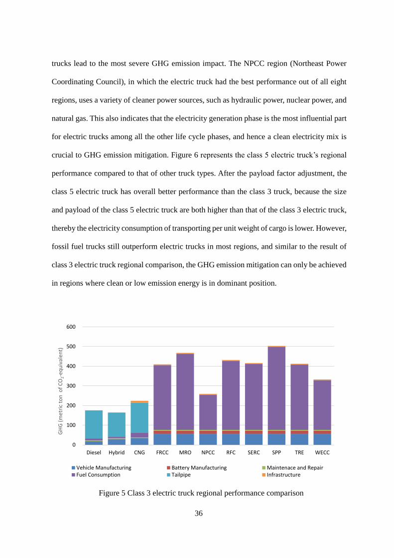
36

trucks lead to the most severe GHG emission impact. The NPCC region (Northeast Power

Coordinating Council), in which the electric truck had the best performance out of all eight

regions, uses a variety of cleaner power sources, such as hydraulic power, nuclear power, and

natural gas. This also indicates that the electricity generation phase is the most influential part

for electric trucks among all the other life cycle phases, and hence a clean electricity mix is

crucial to GHG emission mitigation. Figure 6 represents the class 5 electric truck’s regional

performance compared to that of other truck types. After the payload factor adjustment, the

class 5 electric truck has overall better performance than the class 3 truck, because the size

and payload of the class 5 electric truck are both higher than that of the class 3 electric truck,

thereby the electricity consumption of transporting per unit weight of cargo is lower. However,

fossil fuel trucks still outperform electric trucks in most regions, and similar to the result of

class 3 electric truck regional comparison, the GHG emission mitigation can only be achieved

in regions where clean or low emission energy is in dominant position.

Figure 5 Class 3 electric truck regional performance comparison

0

100

200

300

400

500

600

Diesel Hybrid CNG FRCC MRO NPCC RFC SERC SPP TRE WECC

GH

G (

met

ric

ton

of

CO

2-eq

uiv

alen

t)

Vehicle Manufacturing Battery Manufacturing Maintenace and RepairFuel Consumption Tailpipe Infrastructure

37

Figure 6 Class 5 electric truck regional performance comparison

0

50

100

150

200

250

300

350

Diesel Hybrid CNG FRCC MRO NPCC RFC SERC SPP TRE WECC

GH

G (

met

ric

ton

of

CO

2-eq

uiv

alen

t)

Vehicle Manufacturing Battery Manufacturing Maintenace and Repair

Fuel Consumption Tailpipe Infrastructure

38

3 HYBRID LIFE CYCLE ASSESSMENT OF THE VEHICLE-TO-GRID

APPLICATION IN LIGHT DUTY COMMERICAL FLEET

A partial work of this chapter has been published in the journal of Energy with the title of “A

hybrid life cycle assessment of the vehicle-to-grid application in light duty commercial fleet”

(Zhao and Tatari, 2015)

The Vehicle-to-Grid system is an approach utilizing the idle battery capacity of electric

vehicles while they are parked to provide supplementary energy to the power grid. As

electrification continues in light duty vehicle fleets, the application of Vehicle-to-Grid systems

for commercial delivery truck fleets can provide extra revenue for fleet owners, and also has

significant potential for reducing Greenhouse Gas emissions from the electricity generation

sector. In this study, an economic input-output based hybrid life cycle assessment is conducted

to analyze the potential Greenhouse Gas emissions emission savings from the use of the

Vehicle-to-Grid system, as well as the possible emission impacts caused by battery

degradation. A Monte Carlo simulation is performed to address the uncertainties that lie in the

electricity exchange amount of the Vehicle-to-Grid service as well as the battery life of the

electric vehicles. The results of this study show that extended range electric vehicles and

battery electric vehicles are both viable regulation service providers for saving Greenhouse

Gas emissions from electricity generation if the battery wear-out from regulation services is

assumed to be minimal, but the Vehicle-to-Grid system becomes less attractive at higher

battery degradation levels.

3.1 Introduction and Literature Review

Electricity has a unique nature in that its generation and consumption must take place

simultaneously for it to be truly efficient; otherwise, if the demand for electricity is less than

39

its generation level, the abundant electric power generated is ultimately wasted because, aside

from the limited power storage of hydroelectric pumps, the current power grid has very little

storage capacity (U.S. Energy Information Adiministration, 2000). On the other hand, extra

electricity must be generated on short notice if the peak hour demand exceeds scheduled

generation; this is now mainly accomplished by turning large generators on and off to meet

the fluctuating end user load (Kempton and Tomić, 2005a). Nevertheless, studies have

revealed that electricity storage methods are not only helpful for smoothing out grid

fluctuations in a much shorter response time, but may also be two to three times as effective

as a conventional gas turbine for grid supporting purposes (Makarov et al., 2012)

Although electric passenger cars have undoubtedly the largest capacity potential available,

the willingness of users to provide Vehicle-to-Grid (V2G) services remains unclear, whereas

a small amount of vehicle connection would only add noise to the power grid (Guille and

Gross, 2009). Therefore, this study will use commercial delivery fleet vehicles as its research

objective, as the operation and/or parking times of such fleet vehicles tend to be more

predictable (Tomić and Kempton, 2007). Also, electric truck batteries usually have large

capacities, as 18 light trucks with average outputs of 60 kW are able to provide a maximum

of 1 MW in electricity support (Hill et al., 2012), which is a typical ancillary service contract’s

minimum quantity (Kempton and Tomić, 2005b). Based on this data, a fleet of 20 to 30

electric vehicles would have the potential to be an ancillary electricity provider.

Electricity provided by vehicles has been proven to be far less competitive in the base-load

market than conventional large-scale power plants, which tend to have lower generation costs

(Kempton and Kubo, 2000). Likewise, peak power generation, due to its relatively predictable

pattern, can still be achieved by adjusting generator output. Ancillary services, on the other

hand, accounted for 5% to 10% of electricity costs (a $12 billion market value), and 80% of

40

this payment is made for spinning reserves and/or regulation services (Letendre and Kempton,

2001). The high electricity unit price and the short but rapid power demand requirements of

these ancillary services make V2G a perfect option. However, since spinning reserve services

would require the vehicle(s) in question to be plugged in all the time (Hill et al., 2012), which

may jeopardize the fleet’s normal business operation, this study will only consider the use of

the V2G system for regulation services.

Zhang and his colleagues presented the GHG emission impact and charging cost of electric

vehicles in different operating conditions, and the “smart grid charging” (providing V2G

service) scenario has been proved to be more economically appealing (Zhang et al., 2013).

Kempton et al. (2001) conducted a study comparing the availability and capacity of battery

electric vehicles (BEVs), hybrid electric vehicles (HEVs) and fuel cell vehicles, as well as the

relevant costs of V2G application and the value of the V2G system from the perspectives of

utility companies and customers. The fundamental elements of the V2G system have also

been researched in two different studies in terms of both market availability (Kempton and

Tomić, 2005b) and vehicle owner’s revenue (Kempton and Tomić, 2005a), the former of

which revealed that V2G technologies are highly suitable for electricity ancillary services

(more specifically, regulation services) and also designed and analyzed real life V2G

operation strategies and business models. The latter study offered a quantitative understanding

of the revenues of various types of vehicles as well as how electric vehicles can be

incorporated as part of the grid. Theoretically, BEVs, HEVs and fuel cell vehicles can all be

connected to the grid and provide electric power, but only HEVs and BEVs were considered

in this study because there is no currently available fuel cell vehicle that has power grid

accessibility. Sioshansi and Denholm (2010) simulated the V2G system’s ancillary services

through a unit commitment model and thereby proved its positive effects to the grid and to

41

vehicle fleet owners, demonstrating that HEVs providing grid supporting services take less

time than other vehicle types to repay the initial capital investments.

In addition, an experiment has been performed using a real life HEV for frequency regulation

service (Kempton et al., 2008), during which the regulation signal/value and the battery state

of charge (SOC) during connection were recorded and analyzed. Guille and Gross (2009)

analyzed the features of the V2G system’s components and proposed a possible framework

based on their analysis, as well as possible V2G implementation procedures. The operational

cost as well as benefits of electric vehicles providing V2G services in a smart grid have been

analyzed (Kiviluoma and Meibom, 2011). More specifically, an upcoming EREV has been

studied in terms of commercial truck fleet owners’ economic risks and benefits (Hill et al.,

2012), and scenarios are assumed based on the uncertainty of battery regulation cycle

lifetimes and the unpredictability of regulation signals. Similarly, the integration of electric

commercial fleets to the grid has been proven to be reasonable and profitable (Tomić and

Kempton, 2007). The long-term impact to global energy system and electricity market

brought by V2G application has been explored and discussed (Turton and Moura, 2008).

In addition to the economic aspects covered previously, the GHG reduction potential of

vehicle-to-home (passenger car V2G system) was also studied from a life cycle perspective

(Kudoh et al., 2013), while another study calculated GHG emission impacts in the U.S. based

on various HEV market penetrations with V2G services (Sioshansi and Denholm, 2009).

Battery degradation, as the most important trade off consideration in V2G application, has

also been evaluated in multiple studies: Cicconi and his colleagues summarized the lifetime

of typical vehicle batteries and presented that second-life batteries can be reused in V2G

systems (Cicconi et al., 2012). And the battery degradation caused by V2G service has also

been proved to be minimal (Peterson et al., 2010). The aforementioned literature summarized

42

the feasibility of the V2G system and the roles and functions of HEVs or BEVs within the

system, as well as the positive economic and environmental effects of fleet-level electricity

storage. However, few studies are currently available that have analyzed the GHG emission

impacts caused by integrating V2G technology into a commercial delivery truck fleet. To this

end, this study will conduct an Input-Output based hybrid life cycle assessment with respect

to both EREVs and BEVs, first under a “business as usual” scenario (i.e. without the V2G

system included), and a “V2G regulation service” scenario to simulate the impacts of the V2G

system.

3.2 Method

3.2.1 Scope of the Analysis

The objectives in this session more specifically pertain to HEVs and BEVs. However, the

mass-produced conventional hybrid vehicles have considerably less electric drive power than

mechanical power, and have low capacity batteries (1 to 2 kWh) and no connections to the

grid, making them far less viable than other electric vehicle types as V2G units in the fleet

(Kempton and Tomić, 2005a). On the other hand, EREVs, which have been called the next

generation of hybrid vehicles, have much larger battery capacity (40 kWh) and are advertised

as having a 100-MPG fuel economy (Razer Technologies, 2009). Hence, EREVs and BEVs

have been chosen as the primary research vehicles for this study. According to the scope of

the study defined for this study (Figure 7), the life cycle of the electric truck has been divided

into two phases:

The manufacturing phase, which includes vehicle, battery and charging equipment

manufacturing, fuel/electricity supply production, and vehicle maintenance, and

The operation phase, which represents the fuel consumed by the vehicle’s onboard

43

generator and by the ancillary gas turbine generator.

Figure 7 Scope of the analysis

3.2.2 Vehicle characteristics

Class 3 light duty trucks are normally used for commercial delivery duties; operating in

heavily congested areas during peak traffic hours, these delivery trucks frequently accelerate

and decelerate during operation, and therefore tent to have relatively low fuel economy levels

at about 10 MPG on average, making the electrification of light truck fleets an inevitable trend

in the automotive industry. Multiple public and/or private electric truck fleets have already

been tested, and have proven thus far to have higher fuel economy levels than diesel truck

fleets.

Razer Technologies has developed an advanced plug-in drive system that can be applied to

a light-duty truck platform (Razer Technologies, 2009); the prototype truck can be powered

entirely by its battery for the first 40 miles of travel, which is slightly higher than the typical

daily mileage of a delivery truck. Unlike conventional HEVs, which capture braking energy

or use an internal combustion engine (ICE) after the electric range limit has been reached, this

44

EREV uses a 2-Liter engine (which is much smaller than the displacement size of a normal 6

cylinder light truck) to drive the induction motor, and provide additional driving power. This

“battery-and-generator” combination makes EREVs much more effective than ICE trucks in

terms of fuel consumption. However, the advertised 100-MPG fuel economy of these EREVs

is achieved when the vehicle is unloaded (Kilcarr, 2009); the real life fuel economy will be

discussed further in Section 3.4.1.

For comparison, the Navistar E-star has been selected as the representative BEV for this

study. This all-electric delivery van was first introduced into fleet operations in practice in

2010, and is also advertised to have a diesel-equivalent fuel economy of 100 MPG. The data

used in this study for the BEV was obtained from the two-year Navistar E-star performance

evaluation conducted by the National Renewable Energy Laboratory (National Renewable

Energy Laboratory, 2014a). The general characteristics of these two types of light trucks are

summarized in Table 7.

Table 7 EREV and BEV vehicle characteristics

Extended Range Electric

Vehicle

Battery Electric

Vehicle

Vehicle Make & Model RASER PHEV Drive System Navistar E-star

Curb Weight (lbs.) 5,720.00 7,022.00

Payloads (lbs.) 2,000.00 5,100.00

Battery Capacity (kWh) 40.00 80.00

Fuel Economy (Wh/mile) 843.20 843.20

Vehicle Retail Price

(2014$) 70,000.00 150,000.00

Maintenance Cost(2014$) 0.10 0.07

Pure Electric Range(mile) 20.00 40.00

Infrastructure(2014$) 7,500.00 5,000.00

3.2.3 Scenarios and Initial Assumptions

First, the life cycle assessment of both trucks is conducted under the business-as-usual (BAU)

scenario, meaning that the vehicle in the fleet operates during the day and connects to the grid

45

solely for charging purposes at night. The results of this assessment will then be used as the

reference point for the second assessment, this time with respect to the V2G case, in which

the vehicle operates normally during the day, but is charged to a bidirectional charger at night,

during which time it may provide electricity regulation service to local utility companies.

For the BAU case, the truck is assumed to operate in a fleet of 20 to 30 commercial delivery

trucks, each with an annual mileage of 15,000 miles and a 10 year lifespan before end-of-life

salvaging (Lee et al., 2013b). The 36-month UPS delivery van evaluation (Lammert and

Walkowicz, 2012) indicates that the daily VMT of a parcel delivery truck is about 40 to 50

miles, or 1,400 to 1,700 miles per month; considering the annual mileage assumption

discussed previously, this would assume that each electric truck travels 40 miles per day. A

real life V2G test (Kempton et al., 2008) indicated that a vehicle with identical battery

capacity consumes 36% of its total power storage, while Navistar has a corresponding

consumption rate of about 20% (National Renewable Energy Laboratory, 2014a) because it

has twice as much battery capacity. It is therefore assumed that 40% of the battery storage is

consumed after the truck’s daytime operation, and based on the EREV’s total capacity and

power efficiency (Table 2), the EREV is assumed to have an all-electric range (AER) of 20

miles. This means that, despite the advertised 40-mile AER of the EREV, only half of the

daily range can be powered solely by the battery in reality, while the remaining 20 miles must

be powered by fuel combustion. Likewise, the claimed EREV fuel economy of 100 MPG was,

as stated before, determined from an “unloaded” test; a real life test shows that the fuel

economy of the EREV after the electric range drops to about 50 MPG (Hill et al., 2012), and

another unloaded test of a similar EREV suggests that the minimum fuel economy of the

EREV can be as low as 30 MPG. Hence, considering the real-life payload and the actually

smaller battery capacity, the fuel economy of the EREV after the electric range will be

46

assumed to be 30 MPG.

For the V2G regulation service case, this study will assume that the fleet owner is already

running a business with an electric fleet, and has signed a contract with a local utility company

to provide frequency and/or voltage regulation service. It is considered that these regulation

services will not affect normal delivery operations because of fleet dispatch flexibility,

meaning that the relevant parameters of the daytime operation phase are mostly the same as

in the reference (BAU) case. The available literature shows that delivery fleets usually operate

from 8 a.m. to 8 p.m., so the regulation service period is assumed to be from 8 p.m. on a given

night to 8 a.m. the next day. Furthermore, based on available literature (Turton and Moura,

2008), it is assumed that the onboard fuel is not to be used for regulation service. Likewise,

Kempton and Tomić (2005a) calculated the V2G cost based on the assumption that fuel and

vehicle wear-out only apply to the vehicle operation phase, so it is assumed that the electric

power exchange during regulation service will depend only on the remaining power in the

battery. Furthermore, with respect to the V2G case, two parameters (battery degradation and

regulation up/down signal value) remain unclear in the literature. Since battery degradation is

a deterministic factor of the worth of V2G technology for this application, three scenarios

representing different battery cycle lifetimes are assumed based on current literature, and a

Monte Carlo Simulation will be used to address uncertainties related to regulation signal

values. Both of these uncertainties will be discussed further in Section 3.4.4. All of these

assumptions and general parameters are summarized in Table 8, along with their input data

sources as applicable.

47

Table 8 Assumptions and input data sources

Parameters Unit Value Data Source

EREV

Electricity Efficiency Wh/Mile 843.20

Assumed to be the

same with BEV’s

Fuel Economy MPG 30 See the explanation

above

Maintenance Cost $/Mile 0.10

(Gallo and Tomic,

2013)


(Battery cost

excluded)

$ 50,000 (Hill et al., 2012)

Infrastructure Cost $ 7,500

(U.S. Department of

Transportation, 2012)

BEV

Electricity Efficiency Wh/Mile

843.20

(National Renewable

Energy Laboratory,

2014a)

Maintenance Cost $/Mile 0.07

(Gallo and Tomic,

2013)


(Battery cost

excluded)

$ 110,000 (Feng and Figliozzi,

2013)

Infrastructure Cost $ 5,000 (Gallo and Tomic,

2013)

Others

Producer Price Index - - (US Bureau of Labor

Statistics, 2002);

(U.S. Bureau of Labor

Statistics, 2014)

Diesel Price* $/Gallon 0.78 (Duffy, 2006)

Electricity Price Cent/kWh 7.89 (U.S. Energy

Information

Administration, 2013)

Current Battery Price $/kWh 600 (Gallo and Tomic,

2013)

Future Battery Price $/kWh 450 (Gallo and Tomic,

2013)

3.2.4 Manufacturing phase

The environmental impacts of vehicle manufacturing are derived from the EIO-LCA model,

and the 2002 producer prices (excluding battery price) of the two researched truck types are

calculated as input data. Nevertheless, the available price data consists mostly of vehicle retail

prices, so a producer-retail ratio of 0.8 is assumed for purposes of this study (Samaras and

Meisterling, 2008). Due to their environmentally intensive nature and high manufacturing

48

cost, the impacts and costs of the large capacity battery packs are calculated separately. For

the BAU case, the vehicle battery is assumed to be changed every 150,000 miles

(Electrification Coalition, 2010). Because the inevitably fast charging activity may accelerate

battery degradation, it is assumed that two batteries will be needed during the vehicle’s entire

lifespan. Furthermore, battery price declines due to future large-scale production levels have

also been taken into consideration.

3.2.5 Operation phase and tailpipe impacts

The operation-phase GHG emissions generated by fuel and/or electricity production and by

vehicle maintenance are evaluated as stated before. The maintenance and repair costs for

electric vehicles are considerably lower than those of ICE vehicles because batteries and

motors require little regular maintenance and have fewer fluids (oil, power-steering fluid, etc.)

that need to be changed and/or replaced. Nevertheless, electricity generation is still considered

to be a major pollutant, as power plants are the largest GHG emission sources in the United

States. In order to obtain the lifetime vehicle operation “upstream” impacts, the fuel and/or

electricity consumption and the maintenance cost over each vehicle’s ten-year lifespan are

calculated accordingly. Remember that, as noted in Section 3.4.1, half of the EREV’s total

VMT is powered by electricity, while the other half is powered by onboard fuel consumption.

The tailpipe (i.e. “direct” or “downstream”) emissions are those emissions generated by the

combustion of fossil fuels. These emissions cannot be calculated by the EIO-LCA model, so

a processes-based LCA method is used to account for these impacts instead. The following

equation is used in this study to obtain the tailpipe emissions of the EREV (Hendrickson et

al., 2010):

GHG emission of EREV =𝑉𝑀𝑇

𝑀𝐻𝐹𝐸× 𝐶𝑐𝑜𝑛𝑡𝑒𝑛𝑡−𝑑𝑖𝑒𝑠𝑒𝑙 ×

44

12 ( 5 )

49

Where MHFE is the Metro-Highway Fuel Efficiency, Ccontent-diesel is the carbon content of the

diesel in grams per gallon, and as explained before, the VMT used in this equation is half of

the EREV’s lifetime mileage. On the other hand, the BEV has no tailpipe emissions because

it is powered only by stored electricity, and there is no equation for the oil-powered gas turbine

generator’s direct emissions. The latter of these emissions are therefore calculated as the

product of the amount of electricity generated by gas turbine generators and the generator

emission multiplier (U.S. Energy Information Adiministration, 2015b).

3.2.6 Infrastructure

Although the application of a V2G system to passenger cars may involve additional costs

for home wiring upgrades, such as wiring capacity upgrades and on-board device and

bidirectional interfaces (Kempton and Tomić, 2005b), only limited modifications are needed

to upgrade an existing plug-in electric vehicle system, and centralized charging stations for

commercial fleets may further reduce infrastructure costs (Kempton and Tomić, 2005b).

Based on the summary of multiple studies found in the literature as well as future component

replacement considerations, bidirectional charger costs are assumed to be $7,500 for EREVs

and $5,000 for BEVs. Charging equipment falls under the “Miscellaneous electrical

equipment manufacturing” sector in the EIO-LCA model.

3.2.7 Electricity saving of regulation service and battery degradation

The power grid requires rapid response rates and short duration adjustments as needed to

fine-tune the system voltage and grid frequency while also balancing power generation and

usage. These ancillary services are currently provided via gas turbine generators with typical

response times of 10 to 15 minutes, but with low fuel efficiency and a high GHG emission

factor.

50

The electric vehicles connected to the grid serve as extra energy storage systems, storing

power whenever grid power generation exceeds customer usage (regulation down) and giving

power back to the grid when an additional power boost is needed (regulation up). Nevertheless,

one of the shortcomings of the V2G system is that the rapid electric power exchange may

accelerate the battery degradation. A V2G system test (Kempton et al., 2008) demonstrated

that, during the time that the vehicle is plugged into the grid (8 p.m. to 8 a.m.), about 20 to 30

regulation up/down signals have been received, but the amounts of electricity exchanged and

the corresponding battery degradation levels are still unclear. The assumptions and methods

used in this research to address these two uncertainties are discussed in further detail below.

Firstly, the aforementioned V2G test (Kempton et al., 2008) was conducted for a passenger

car with a battery capacity of 40 kWh, which is the same as the battery capacity assumed for

the EREV in this study, and approximately 30 regulation up/down cycles can be observed

from the data record for this study. Although the electricity demand of a region can be

predicted based on hourly or seasonal historical patterns, the regulation signal characteristics

(positive or negative) and regulation request values have been described in the literature as

“unpredictable” (Kempton and Tomić, 2005b), and the real-life V2G system test also shows

a random request record (Kempton et al., 2008), because the grid frequency and voltage are

affected by the turning on and turning off of millions of the appliances. The PJM regional

electricity demand pattern (PJM Interconnection LLC, 2015) and single-user level regulation

signal are shown in Figure 8.

51

Figure 8 PJM average 24-hour electricity demand (a) PJM regulation signal (b)

Although regional regulation market data is available (PJM Interconnection LLC, 2014),

there is few regulation signal data available at an individual regulation service provider level.

However, it is clear that regulation requirements are due to seasonal and daily grid load

patterns (Kirby, 2005), meaning that a regulation up signal will be triggered if there is a sudden

increase in electricity usage, while a sudden decrease in power consumption will result in a

regulation down signal. Therefore, during a 12-hour connection period, the following

regulation signal patterns will be assumed:

High-Demand Periods: 20 regulation up and 10 regulation down signals;

Moderate-Demand Periods: 15 regulation up and 15 regulation down signals; and

0

1000

2000

3000

4000

5000

1 2 3 4 5 6 7 8 9 10 11 12 13 14 15 16 17 18 19 20 21 22 23 24PJM

Reg

ion

al L

oad

(M

W)

Time

PJM Regional 24 Hour Electricity Load

-1.5

-1

-0.5

0

0.5

1

1.5

2

20

:00

20

:30

21

:00

21

:30

22

:00

22

:30

23

:00

23

:30

0:0

0

0:3

0

1:0

0

1:3

0

2:0

0

2:3

0

3:0

0

3:3

0

4:0

0

4:3

0

5:0

0

5:3

0

6:0

0

6:3

0

7:0

0

7:3

0

8:0

0

Reg

ula

tio

n R

equ

est

(KW

)

Regulation Signal Received by the Individual Service Provider

52

Low-Demand Periods: 10 regulation up and 20 regulation down signals.

The demand level, on the other hand, can be determined from the 10-month U.S. electricity

demand data provided by the U.S. Energy Information Administration (U.S. Energy

Information Administration, 2011). To match the time period of this study, the hourly-based

U.S. electricity demand data are extracted for the time period from 8 p.m. to 8 a.m. It can be

observed that almost all of the 3,648 electricity demand data points within this period tend to

range from 10,000 MW to 15,000 MW. After sorting these data points, it was found that 1,577

points fall below the average electricity demand (12,500 MW), 1,149 points lie between

12,500 MW to 15,000 MW, and only 922 points are larger than 15,000 MW demand level. It

is therefore concluded that 43% of the total nighttime in a single year consists of low power

demand levels, while the corresponding percentages are 32% for moderate demand and 25%

for high demand. To validate this conclusion, The PJM (RTO of 13 states and District of

Columbia) detailed historical regulation signal data has been randomly sampled and

calculated as appropriate; the results indicate a distribution of 50% regulation down (negative)

signal levels, 35% moderate regulation up (positive) signal levels, and 15% high regulation

up signal levels, meaning that the demand levels previously assumed are adequate.

Another uncertainty factor that affects the total electricity exchange during regulation

services is the requested amounts of power demand (positive or negative) in each regulation

cycle. The literature thus far has used an average regulation demand of 1.30 kWh per

regulation up cycle and 0.88 kWh per regulation down cycle (Hill et al., 2012). However, to

improve calculation accuracy, the regulation up and regulation down values (measured in kW)

are extracted along with their corresponding regulation periods (measured in hours) as

variables with uncertainties from the test conducted by Kempton et al. (2008). To adequately

reflect the uncertainties connected to the regulation signals, a Monte Carlo Simulation is

53

applied separately with respect to the extracted regulation up and down data sets. Therefore,

instead of presenting the ultimate GHG emission savings as a fixed value, these savings will

be represented by probability intervals.

Per the assumptions discussed previously, 40% of the stored electricity is consumed during

daytime delivery operations. Kempton and Tomić (2005a) used similar assumptions in their

study (i.e. 50% of the battery is depleted before V2G connection), so this study will assume

that the battery’s State of Charge (SOC) is 60% when the battery is plugged in for regulation

service., Table 9 summarizes the battery SOCs under different power demand situations and

the electricity amounts provided by the vehicle, based on the average (most likely) results

from the aforementioned Monte Carlo Simulation. The lifetime electricity savings (and, in

turn, the GHG emission impact savings) can then be calculated by combining the demand

level possibilities mentioned above, with an additional 10% charging energy loss and a 7%

discharging energy loss included in these calculations as well (Sioshansi and Denholm, 2010).

As shown in Table 9, there is a possibility that the vehicle can actually gain electricity during

regulation provision time, meaning that less electricity is needed to recharge the battery to its

full capacity.

54

Table 9 Regulation service data

Demand Level Regulation

Up Cycles

Regulation

Down Cycles

EREV Energy

Storage before

Service (kWh)

EREV Energy

Storage after

Service (kWh)

EREV SOC

after

Regulation

Service

Electricity

Provided by

EREV

(kWh)

High-demand 20 10 24 18.1 45.25% 11.0

Moderate-

demand

15 15 24 23.4 58.50% 8.3

Low-demand 10 20 24 28.7 71.75% 5.5

High-demand 20 10 48 42.1 52.63% 11.0

Moderate-

demand

15 15 48 47.4 59.25% 8.3

Low-demand 10 20 48 52.7 65.88% 5.5

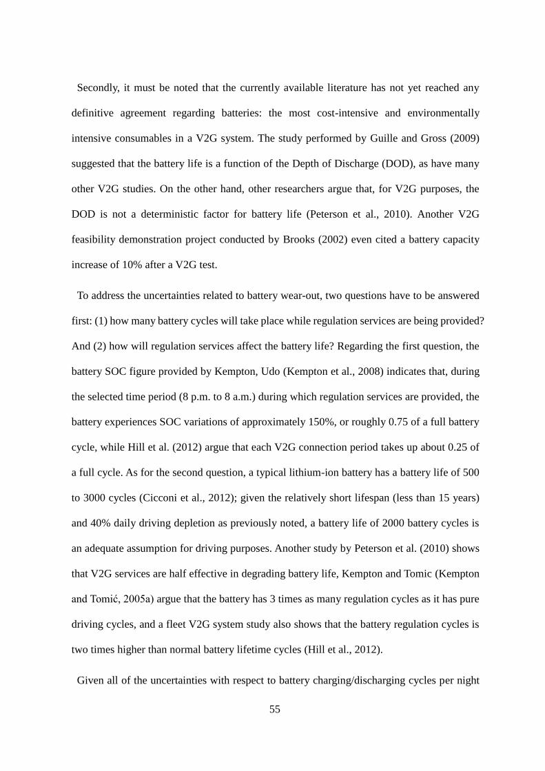
55

Secondly, it must be noted that the currently available literature has not yet reached any

definitive agreement regarding batteries: the most cost-intensive and environmentally

intensive consumables in a V2G system. The study performed by Guille and Gross (2009)

suggested that the battery life is a function of the Depth of Discharge (DOD), as have many

other V2G studies. On the other hand, other researchers argue that, for V2G purposes, the

DOD is not a deterministic factor for battery life (Peterson et al., 2010). Another V2G

feasibility demonstration project conducted by Brooks (2002) even cited a battery capacity

increase of 10% after a V2G test.

To address the uncertainties related to battery wear-out, two questions have to be answered

first: (1) how many battery cycles will take place while regulation services are being provided?

And (2) how will regulation services affect the battery life? Regarding the first question, the

battery SOC figure provided by Kempton, Udo (Kempton et al., 2008) indicates that, during

the selected time period (8 p.m. to 8 a.m.) during which regulation services are provided, the

battery experiences SOC variations of approximately 150%, or roughly 0.75 of a full battery

cycle, while Hill et al. (2012) argue that each V2G connection period takes up about 0.25 of

a full cycle. As for the second question, a typical lithium-ion battery has a battery life of 500

to 3000 cycles (Cicconi et al., 2012); given the relatively short lifespan (less than 15 years)

and 40% daily driving depletion as previously noted, a battery life of 2000 battery cycles is

an adequate assumption for driving purposes. Another study by Peterson et al. (2010) shows

that V2G services are half effective in degrading battery life, Kempton and Tomic (Kempton

and Tomić, 2005a) argue that the battery has 3 times as many regulation cycles as it has pure

driving cycles, and a fleet V2G system study also shows that the battery regulation cycles is

two times higher than normal battery lifetime cycles (Hill et al., 2012).

Given all of the uncertainties with respect to battery charging/discharging cycles per night

56

and battery regulation cycles, this study assumes three different battery wear-out scenarios for

both vehicle types, as summarized in Table 10. The first scenario represents the least battery

wear-out, with one regulation cycle equal to 1/4 driving cycle while the battery also has the

longest regulation life. The second scenario represents a mid-level wear-out effectiveness and

an average battery regulation life. Lastly, the third scenario represents the maximum possible

battery wear-out due to regulation service. The last column of Table 10 indicates the number

of additional batteries needed under each scenario to compensate for providing regulation

services.

Table 10 Battery regulation life cycle scenarios and battery numbers

Battery Scenarios

Cycles

per

Night

Battery

Regulation

Life

Number

of Extra

Battery

EREV

Battery

Scenarios

Minimum Battery Wear Out 0.25 6000 0

Medium Battery Wear Out 0.75 4000 1

Maximum Battery Wear Out 1 2000 2

BEV Battery

Scenarios

Minimum Battery Wear Out 0.125 6000 0

Medium Battery Wear Out 0.375 4000 0

Maximum Battery Wear Out 0.5 2000 1

* The BEV uses only half as many cycles as the EREV, because the BEV’s battery capacity

is twice as much as that of the EREV

3.3 Results

The assessment results are shown in Figure 9. Figure 9a compares the life cycle GHG

emissions of the EREV and the BEV under BAU conditions, with regulation services not

included. This figure indicates that, in a business-as-usual case, the GHG emission impacts of

the BEV are almost twice as much as those of the EREV in terms of vehicle/battery

manufacturing and electricity supply. This is because BEV manufacturing requires large

amounts of light-weighted materials and large-capacity battery packs, so the overall

manufacturing cost is higher than those of EREVs or conventional fossil-fuel powered

vehicles, although the larger battery capacity of the BEV affords it a higher payload and longer

57

AER than the EREV. The lifetime maintenance and infrastructure impacts for both truck types

are relatively lower than those of other life cycle phases, and are identical for both trucks,

except that the BEV has no fossil-fuel related emissions thanks to its all-electric power system.

It should also be noted that, unlike traditional hybrid trucks with powertrain still mostly reliant

on fuel combustion, the EREV’s main power source is electricity, making the EREV’s tailpipe

emissions considerably lower than those of diesel powered trucks.

Figures 9b through 9d illustrate the life cycle GHG emissions of the two truck types when

V2G regulation services are provided, with each figure represents the vehicles’ environmental

performances with low, average, and high levels of battery wear-out, respectively. The

negative electricity saving values in each of these figures indicate a net savings in GHG

emissions from providing regulation services. Taking the most likely Medium Battery Wear-

Out scenario (Figure 9c) as an example, the vehicle receives electricity during charging and,

through the use of V2G regulation services, may then give electrical power back to the grid

for voltage stabilizing as necessary, reducing the amount of electricity that would otherwise

need to be generated by gas turbines and thereby “saving” approximately 40 tons of GHG

emissions from regulation services. Moreover, the emission savings results in Figures 9b

through 9d are shown after multiplying the initial result by two because, as noted before,

electricity storage methods are twice as effective as electricity generation in terms of ancillary

service (Lin, 2011). In short, for every 1 MW of electricity provided by V2G services, a gas

turbine regulation service would need to consume enough fuel to provide 2 MW of electricity.

A parallel comparison among Figures 9b through 9d shows that the emission impacts of

battery manufacturing increase significantly as the degree of battery wear-out aggravates. The

error bars on the “electricity savings” and “electricity supply” columns in each figure

represent the results of the Monte Carlo Simulation as previously discussed, with the two

58

extreme values on each error bar indicating the possible maximum and minimum impact

values, while the column value indicates the average (i.e. most likely) impact value. In Figure

9b (low battery wear-out), the battery degradation impacts of both electric vehicles are less

than their respective emission savings, indicating a net savings in GHG emissions. The results

based on medium battery wear out (Figure 9c) show that, although the EREV’s battery

manufacturing emissions are still less than the environmental benefits of regulation services,

the corresponding benefits for the BEV are almost offset by the BEV’s battery wear out.

Finally, in Figure 9d (high battery wear-out), the EREV can still serve as a V2G regulation

service provider, but the large amount of GHG emissions from battery manufacturing exceeds

the EREV’s electricity emission savings. Furthermore, given the uncertainties with respect to

regulation services, the BEV as a V2G provider is still hardly an eligible option if the

maximum level of battery wear-out is assumed, as the BEV’s average electricity supply

emissions are roughly equivalent to its electricity emission savings. Furthermore, the error

bars in Figure 9 all have wide ranges, which also suggests that the electricity exchange

amounts of each regulation cycle and regulation request frequencies will also have a

significant effect on the total electricity emission savings

However, when comparing Figure 9a to either Figure 9b, 9c, or 9d, it becomes clear that the

inclusion of the V2G system significantly reduced the electricity supply emissions for both

vehicle types. This is because, due to the inherently unpredictable regulation signals, the

vehicle battery can be either depleted to a certain SOC or fully charged by the end of the night,

so there is a possibility that the total electricity inflow is larger than the total outflow, in which

case the net electricity gain can be considered as “free energy”. Furthermore, the relatively

small error bars on the electricity supply columns of Figures 9a through 3d show that

electricity supply emissions tend to be stable with or without the V2G system.

59

Figure 9 Life-cycle GHG emissions (a) BAU (b) V2G with low battery wear-out (c) V2G with mid-level battery wear-out (d) V2G with

high battery wear-out

60

4 ECONOMIC AND ENVIRONMENTAL BENEFIT ANAYSIS OF

VEHICLE-TO-GRID SERVICES PROVIDED BY ELECTRIC DELIVERY

TRUCKS

A partial work of this chapter has been published in the journal of Applied Energy with the

title of “Vehicle to Grid regulation services of electric delivery trucks: Economic and

environmental benefit analysis” (Zhao et al., 2016a)

Concerns regarding the fuel costs and climate change effects associated with petroleum

combustion are among the main driving factors for the adoption of electric vehicles. Future

commercial delivery truck fleets may include BEVs and EREVs; in addition to savings on

fuel and maintenance costs, the introduction of these grid accessible electric vehicles will also

provide fleet owners with possible V2G opportunities. This section investigates the potential

net present revenues and GHG emission mitigation of V2G regulation services provided by

electric trucks in a typical fleet. The total cost of ownership and the life-cycle GHG emissions

of electric trucks are also analyzed and compared to those of traditional diesel trucks. To

account for uncertainties, possible ranges for key parameters are considered instead of only

considering fixed single data values for each parameter.

4.1 Introduction and Literature Review

EVs have proven to have significant environmental impact mitigation potential if the local

electricity sources are renewable (esp. hydropower or wind power). More importantly, Vehicle

to Grid (V2G) systems, a further integration of electric power grids and EVs, utilize the

battery capacity of idled EVs as grid storage, allowing them to improve the reliability of the

power grid, reduce GHG emission impacts as opposed to the low-efficiency operation of

61

traditional power plants, provide additional revenue for vehicle/fleet owners, and help to

promote the implementation of clean energy and to further increase the market penetration of

EVs. However, despite the benefits that V2G technologies provide, the implementation of this

relatively new concept may face economic or sociological problems (Sovacool and Hirsh,

2009). To explore the feasibility of the application of V2G systems, this article will evaluate

the GHG emission savings and potential revenues for fleet operators using EREVs or BEVs

as V2G regulation service providers. The system boundary will follow the most cited studies

(Kempton and Tomić, 2005a, b; Kempton et al., 2001; Tomić and Kempton, 2007), including

fuel/electricity production phase, battery manufacturing phase and V2G-related vehicle

operation phase, which is the main focus of this study. Vehicle manufacturing and end-of-life

disposal will not be involved considering that these two phases have no effect on V2G-related

analysis. On the other hand, V2G regulation services may accelerate the degradation of

batteries and battery manufacturing and disposal are emission intensive, hence, battery

degradation scenarios will also be analyzed in detail. To address the spatial differences and

uncertainties of the parameters, the research will be conducted in five Independent System

Operator (ISO) and Regional Transmission Organization (RTO) regions, and the resulting

revenues and life cycle emission savings will be projected for 15 years (2016-2030). The

methods as well as calculations used in this study are shown in Figure 10.

62

Figure 10 Framework of the model

The feasibility and benefits of electric drive vehicles providing ancillary services have been

studied by Kempton et al. (Kempton et al., 2001). Their study answered the fundamental

question as to the best practical application of V2G systems; instead of generating electricity

as a power source, the value of the V2G system is that, as a storage media, it allows the grid

operator to control the precise timing of the valuable electricity flows into or out of the grid.

Therefore, as a grid stabilizer, the V2G system’s main economic drive is the high value of the

electricity that it processes. As we all know, renewable energy sources (wind, solar, etc.) are

subject to a great deal of fluctuation as the availability of these sources cannot be predicted

accurately for any given time period, and one promising application of the V2G system is to

more closely integrate with renewable energy sources (Lund and Kempton, 2008). Kempton

and Tomic conducted a separate study further exploring the actual available power of the

vehicle, as well as V2G regulation service revenue and the effects of battery degradation

(Kempton and Tomić, 2005a), and in another study, they also evaluated real-life

implementation strategies for V2G technologies, possible business models, and the most

valuable application of V2G systems, i.e. incorporating them with clean but highly fluctuating

renewable energy sources (Kempton and Tomić, 2005b). Zhong et al. proposed a coordinated

63

control strategy for AGC that involves large-scale electric vehicle charging/ discharging

(Zhong et al., 2014). Similarly, an optimal charging scheduling model has been developed by

Jian et al. (Jian et al., 2015). As the EV market penetration increase in the future, the impact

of connecting these EVs into the grid has been studied by Foley et al. (Foley et al., 2013).

Noel and McCormack studied the potential savings in ownership costs via V2G services,

which are the main drive for fleet operators to adopt EVs and the V2G system (Noel and

McCormack, 2014). PHEVs, BEVs, and fuel cell vehicles have been researched in all of the

aforementioned studies, but not all of these vehicle types are practical or available for light

duty trucks; for instance, fuel cell vehicles as V2G service providers may face challenges such

as grid accessibility, hydrogen storage and conversion losses (Hu et al., 2015b). On the other

hand, an advanced plug-in hybrid vehicle, the EREV, has been introduced and studied at a

delivery fleet level (Hill et al., 2012). Within this study, light duty truck fleets serve as

functional units providing regulation services, and the fleet as a whole proved to be more

feasible than private cars as V2G providers. Kempton et al. have also performed a real-life

experiment testing the behavior of EV batteries in response to PJM regulation requests,

recording the random signal patterns of the regulation requests as well as the shallow

charge/discharge patterns of the battery.

In addition to the economic aspects of V2G systems, the environmental benefits of such

systems have also been studied in the literature. An energy-system model was used to project

the long term transformation of both energy and transportation systems from the use of a V2G

system, as well as the resulting GHG emission savings (Turton and Moura, 2008). The Life

Cycle Assessment (LCA) method has been widely used as a tool to analyze the environmental

impact of a product or process over its lifetime (Ercan et al., 2015). Kudoh et al. studied one

V2G application, the Vehicle-to-Home system, from a LCA perspective, and the result showed

64

significant emission savings (Kudoh et al., 2013).

Battery degradation is the most potentially troublesome downside of V2G services, and as

such it has been discussed in multiple studies. Cicconi et al. summarized the life cycles of

typical vehicle batteries and argued that second-life batteries are actually good options for

V2G services (Cicconi et al., 2012), and in fact Peterson et al. proved that the battery wear-

out due to regulation services is minimal (Peterson et al., 2010). Although regulation up

(power request from the grid) and regulation down (storage of excess power) signals are rapid

and repeated, the Battery State of Charge (SOC) variation in each regulation cycle is fairly

small. Therefore, most studies in current literature agree that the degradation effects of V2G

services on EV batteries is minimal (Bishop et al., 2013). Nevertheless, in addition to battery

degradation-related cost issues, V2G contract issue may reduce customers’ willingness to

adopt V2G technologies (Hidrue and Parsons, 2015), there are many other sociological,

economic or behavioral problems that may prevent the implementation of V2G systems

(Sovacool and Hirsh, 2009). The effects of these problems will be further discussed in later

sections. The aforementioned literature summarizes the framework of the V2G system, the

roles of EVs in this framework, and the potential economic and environmental benefits of this

system. However, light duty delivery truck fleets, as a promising first-step V2G service

provider, have not been studied from a life cycle perspective, and few studies are currently

available that have projected the future economic and environmental effects brought by light

duty trucks as V2G service providers in different regions. To this end, this study will analyze

the life cycle revenue/cost of V2G regulation services provided by BEVs and EREVs in five

ISO/RTO regions, and as the key parameters such as fuel and electricity price changes in the

future, these spatial results will be projected for the next 15 years. In addition, life cycle

environmental impact saving and economic benefits will be compared among BEVs, EREVs

65

and ICVs, and with the consideration such as federal and state incentives and potential carbon

tax scenarios, decision makers in various ISO/RTO regions will be provided a holistic

evaluation of V2G regulation services carried out by light duty electric trucks. Furthermore,

in addition to the lack of forecast and spatial research, single data points are usually used as

key parameters in the aforementioned studies, yet in real lives, these key parameters may vary

within certain ranges. So the most important feature of this study is that instead of using fixed

values, applicable ranges are applied to all key parameters to account for uncertainties.

4.2 Delivery Truck Fleets as Grid Storage Providers

Although the use of passenger cars as a whole has undoubtedly the largest capacity potential,

the relatively smaller battery capacities of passenger cars limits their feasibility as V2G

service providers, as such a small amount of connection is merely a “noise” to the grid (Guille

and Gross, 2009). Hence, aggregators are needed to coordinate large amounts of EVs in a

particular area, meanwhile the willingness of EV owners to provide V2G services still remains

unclear. Commercial delivery truck fleets may therefore be a better preliminary application

of V2G technologies, for a variety of reasons:

Capacity: The batteries of electric trucks have higher capacities and higher energy outputs

than electric passenger cars. Typical electric truck battery capacities range from 80 kWh to

120 kWh per truck, and a delivery fleet of 18 trucks with average outputs of 60 kW each are

able to provide a maximum capacity support of 1 MW (Hill et al., 2012), which is the

minimum required capacity of a typical ancillary service contract (Kempton and Tomić,

2005b). For this reason, a fleet of 20 to 30 PHEVs or BEVs would be feasible as an individual

ancillary service provider.

Centralized Coordination: Delivery trucks commonly operate from 8 a.m. to 8 p.m., and

these relatively predictable fleet operation schedules as opposed to those of passenger cars

66

make delivery trucks a better option in terms of system reliability. Moreover, the centralized

charging stations at the depot where the trucks are parked when not in use would require lower

infrastructure/upgrade costs overall (Kempton and Tomić, 2005b).

Rational Decision Making: Individual passenger car buyers often choose traditional vehicles

over EVs based on considerations regarding the shape, color, and/or interior comfort of a

passenger vehicle, whereas fuel economy and environmental impacts are seldom given any

significant priority when purchasing a passenger vehicle (Sovacool and Hirsh, 2009). Fleet

operators, on the other hand, have to more seriously consider fuel consumption rates and GHG

emission levels as priorities for socio-economic and environmental reasons. Taking the

frequent stop-and-go operational nature of electric delivery trucks into consideration,

although electric trucks require high initial cost, the environmental impact during the

operation phase is much less than that of traditional diesel trucks, and providing V2G services

may give fleet owners an additional source of revenue that can offset operation costs.

No Range Anxiety: When calculating power availability for V2G provision, the buffering

range has to be taken into consideration for car owners due to their relatively unpredictable

operation patterns. On the other hand, delivery trucks normally operate on fixed routes. Hence,

this range anxiety does not exist for delivery trucks, and so the buffering range need not be as

large for delivery trucks as for passenger cars.

Electricity provided through the combustion of the vehicle on-board fuel has proven to be

far less competitive than base-load electricity, which is generated by large-scale power plants

and tend to have lower generation costs and emission rates (Kempton and Kubo, 2000).

Likewise, peak power, due to its relatively predictable demand patterns, can still be generated

by ramping up power plants. However, ancillary services account for 5% to 10% of the total

electricity market value (about $12 billion) (Letendre and Kempton, 2001), have the highest

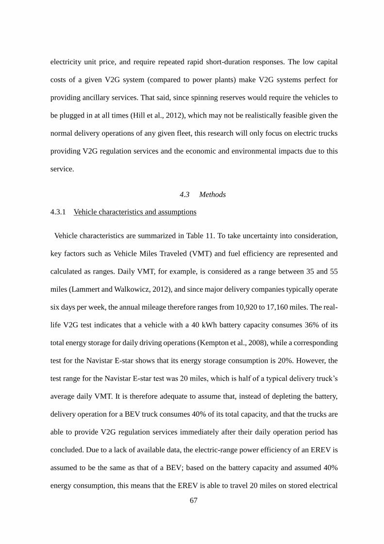
67

electricity unit price, and require repeated rapid short-duration responses. The low capital

costs of a given V2G system (compared to power plants) make V2G systems perfect for

providing ancillary services. That said, since spinning reserves would require the vehicles to

be plugged in at all times (Hill et al., 2012), which may not be realistically feasible given the

normal delivery operations of any given fleet, this research will only focus on electric trucks

providing V2G regulation services and the economic and environmental impacts due to this

service.

4.3 Methods

4.3.1 Vehicle characteristics and assumptions

Vehicle characteristics are summarized in Table 11. To take uncertainty into consideration,

key factors such as Vehicle Miles Traveled (VMT) and fuel efficiency are represented and

calculated as ranges. Daily VMT, for example, is considered as a range between 35 and 55

miles (Lammert and Walkowicz, 2012), and since major delivery companies typically operate

six days per week, the annual mileage therefore ranges from 10,920 to 17,160 miles. The real-

life V2G test indicates that a vehicle with a 40 kWh battery capacity consumes 36% of its

total energy storage for daily driving operations (Kempton et al., 2008), while a corresponding

test for the Navistar E-star shows that its energy storage consumption is 20%. However, the

test range for the Navistar E-star test was 20 miles, which is half of a typical delivery truck’s

average daily VMT. It is therefore adequate to assume that, instead of depleting the battery,

delivery operation for a BEV truck consumes 40% of its total capacity, and that the trucks are

able to provide V2G regulation services immediately after their daily operation period has

concluded. Due to a lack of available data, the electric-range power efficiency of an EREV is

assumed to be the same as that of a BEV; based on the battery capacity and assumed 40%

energy consumption, this means that the EREV is able to travel 20 miles on stored electrical

68

power alone. After the all-electric range has been used up, the advertised diesel fuel efficiency

of 100 MPG was, as stated before, determined from an unloaded test; a corresponding real-

life test shows that the fuel efficiency drop to 50 MPG (Hill et al., 2012) when the truck was

loaded, and another discussion of a similar EREV indicates that this fuel efficiency can drop

to as low as 30 MPG (Kilcarr, 2009). Therefore, the fuel efficiency of the EREV’s all-electric

range is assumed to range from 30 to 50 MPG. Since all delivery trucks operate on relatively

fixed routes, it is assumed that no buffering range is needed for either of these trucks.

The variable Pvehicle is an important factor measuring the power output level of a vehicle.

Based on Kempton and Tomic’s study (Kempton and Tomić, 2005a), Pvehicle is calculated using

Equation 6:

𝑃𝑣𝑒ℎ𝑖𝑐𝑙𝑒 = (𝐵𝑐𝑎𝑝 −

𝐷𝑑 −𝐷𝑏𝑢𝑓𝑓𝑒𝑟

𝐹𝑒 ) 𝐶𝑒

𝑇𝑑𝑖𝑠𝑝

(6)

Where Bcap is the capacity of the vehicle battery, Dd is the average Daily VMT (45 miles),

Dbuffer is the minimum backup range required for each EV, Fe is the fuel efficiency of each EV

in miles/kWh, Ce is the electricity conversion efficiency (90% for grid-to-battery power and

93% for battery-to-grid power) (Sioshansi and Denholm, 2010), and Tdisp is the effective

regulation provision time (usually assumed to be 20 minutes) (Kempton and Tomić, 2005a).

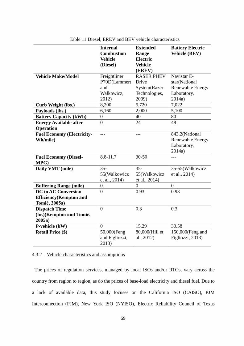
69

Table 11 Diesel, EREV and BEV vehicle characteristics

Internal

Combustion

Vehicle

(Diesel)

Extended

Range

Electric

Vehicle

(EREV)

Battery Electric

Vehicle (BEV)

Vehicle Make/Model Freightliner

P70D(Lammert

and

Walkowicz,

2012)

RASER PHEV

Drive

System(Razer

Technologies,

2009)

Navistar E-

star(National

Renewable Energy

Laboratory,

2014a)

Curb Weight (lbs.) 8,200 5,720 7,022

Payloads (lbs.) 6,160 2,000 5,100

Battery Capacity (kWh) 0 40 80

Energy Available after

Operation

0 24 48

Fuel Economy (Electricity-

Wh/mile)

--- --- 843.2(National

Renewable Energy

Laboratory,

2014a)

Fuel Economy (Diesel-

MPG)

8.8-11.7 30-50 ---

Daily VMT (mile) 35-

55(Walkowicz

et al., 2014)

35-

55(Walkowicz

et al., 2014)

35-55(Walkowicz

et al., 2014)

Buffering Range (mile) 0 0 0

DC to AC Conversion

Efficiency(Kempton and

Tomić, 2005a)

0 0.93 0.93

Dispatch Time

(hr.)(Kempton and Tomić,

2005a)

0 0.3 0.3

P-vehicle (kW) 0 15.29 30.58

Retail Price ($) 50,000(Feng

and Figliozzi,

2013)

80,000(Hill et

al., 2012)

150,000(Feng and

Figliozzi, 2013)

4.3.2 Vehicle characteristics and assumptions

The prices of regulation services, managed by local ISOs and/or RTOs, vary across the

country from region to region, as do the prices of base-load electricity and diesel fuel. Due to

a lack of available data, this study focuses on the California ISO (CAISO), PJM

Interconnection (PJM), New York ISO (NYISO), Electric Reliability Council of Texas

70

(ERCOT), and ISO New England (ISONE) regions, all of which are illustrated in Figure 11.

Figure 11 ISO/RTO regions

The data assumptions and uncertainty ranges of the V2G system are summarized in Table

12.

71

Table 12 Preliminary assumptions and data sources

Parameter Source Range, Distribution, or Data

Source

Analysis Period (Noori et al., 2015) 2016-2030

Discount Rate (Bankrate, 2014) 0.65%-1.15%

Inflation Rate (CBO, 2014) -10%, +10% of CBO’s projections

Electricity Price (U.S. Energy Information

Administration, 2014)

EIA & proposed method in (Noori et

al., 2015)

Diesel Price (U.S. Energy Information

Adiministration, 2015a)

EIA diesel price projections from

2016 to 2030 in the five researched

regions

Battery Lifetime,

Production &

Recycling Emissions

(Amarakoon et al., 2013) Battery lifetime presented in Section

4.3.3

Battery related emissions, Presented

in Section 4.3.8

Average Vehicle

Lifetime

(Barnitt et al., 2010) 15 years

Vehicle Purchase

Price

- Presented in Table 4.

Pricecap (Tomić and Kempton, 2007),

(Kempton et al., 2008)

Presented in Section 4.3.4

Priceele (Noori et al., 2015) Presented in Section 4.3.4

Tplug (Hill et al., 2012) 8 to 12 hours per day

Tcyc (Kempton et al., 2008) Uniform (3.6, 9) minutes

Pline (Kempton and Tomić, 2005a) 19.2 kW to 25 kW, Presented in

Section 4.3.5

Ndisp (Kempton et al., 2008) Uniform (30, 40) times

Battery Lifetime

Cycles for Regulation

Services

(Kempton and Tomić, 2005a),

(Peterson et al., 2010), (Hill et

al., 2012)

Uniform (2,000 to 6,000) cycles,


Depth of Discharge (Kempton and Tomić, 2005b) Uniform (3, 10)

Battery Price (Gallo and Tomic, 2013) (600 - year x 30) x battery capacity,


Battery Capacity (Razer Technologies, 2009),


Laboratory, 2014a)

EREV 40 kWh

BEV 80 kWh

Battery to Grid

Efficiency

(Sioshansi and Denholm,

2010)

0.93 x 0.9

V2G charger cost

and upgrade cost

(Kempton and Tomić, 2005a),

(Gallo and Tomic, 2013)

Charger: $5000

Equipment Upgrade: Uniform

($1,900 to $2100)

Battery Lifetime (Electrification Coalition,

2010), (Cicconi et al., 2012)

5 to 10 years, Presented in Section

4.3.3

Grid Electricity

Emission


2013), (U.S. Environmental

Protection Agency, 2014b),

(U.S. Energy Information

Adiministration, 2015d)

-10%, 10% of the projected values


Traditional

Regulation Service

Emission

(Lin, 2011), (Makarov et al.,

2012)

2-3 times of gas turbine power plant

emissions


72

4.3.3 Battery degradation costs due to driving and V2G service provision

Based on the literature (Electrification Coalition, 2010), the battery of an electric truck is

supposed to be replaced after every 150,000 miles of travel; based on the daily VMT range

assumed for this study, this means that the battery must be changed approximately every 10

years. Another study argues that some vehicle batteries are able to last 15 years, but the actual

battery capacity is often lower than the officially stated capacity, and other external factors

such as fast charging or low-temperature environments may further reduce the lifetime of a

vehicle battery. From a life cycle perspective, a typical lithium-ion battery has a total battery

life of 500 to 3000 cycles (Cicconi et al., 2012). Given the conservative lifespan assumption

of less than 15 years and the 40% daily energy consumption as previously noted, a battery life

of 2,000 cycles (driving only) is an adequate assumption. Therefore the life span can be

approximately computed as 2,000 / (52 x 6) = 6.4 years. Hence, the battery lifespan of the

truck is assumed to range from 5 to 10 years. In addition to the battery degradation caused by

normal operation, V2G regulation services will also accelerate battery wear-out, but as

previously noted, the battery degradation incurred from V2G services is less than that caused

by daily driving. In short, after summarizing the literature (Hill et al., 2012; Kempton and

Tomić, 2005a; Peterson et al., 2010), the total battery life cycle for V2G regulation services

alone is assumed to be 2,000 to 6,000 cycles.

When calculating the total cost of ownership, battery replacement costs must be considered

when each battery reaches its life span. The unit price of the battery is predicted to decrease

in the future, from $600/kWh in 2015 to $450/kWh 2020 and then to $300/kWh in 2025 (Gallo

and Tomic, 2013). This trend indicates a linear decrease in battery unit prices, with prices

starting at $600/kWh in the year 2015 and then decreasing by $30/kWh per year. Labor cost

uncertainties have also been included in these calculations, with unit prices ranging from

73

$30/hour to $40/hour while work hours range from 7 to 13 hours per day.

The aforementioned battery replacement cost is caused by the normal operation of delivery

trucks, but V2G services will also incur battery wear-out and thereby increase the total cost.

Kempton and Tomic’s method for calculating V2G-related battery degradation costs

(Kempton and Tomić, 2005a), as summarized in Equations 15 through 17, will be applied in

this study.

4.3.4 Electricity price

The Electric Vehicle Regional Optimizer (EVRO) model previously developed by the

authors to calculate the electricity cost (Noori et al., 2015), Priceele, is used in this study as

well. EVRO is an optimization model that uses several previously established methodologies

in Life Cycle Assessment of energy systems, Multi Criteria Decision Making (Nam, 2014;

Noori et al., 2013), Decision Making Under Uncertainty (Noori, 2013), Intelligence

Transpiration Systems (Al-Deek et al., 2014), Stochastic Optimization (Kucukvar et al.,

2014b; Noori et al., 2014), and builds on the Argonne National Lab’s Alternative Fuel Life-

Cycle Environmental and Economic Transportation (AFLEET) model (AFLEET, 2013) to

estimate several specifications related to EVs in a regional basis. Figure 12 shows the

estimated prediction of the levelized cost of electricity for each of the considered U.S. electric

regions. These estimates are used to calculate the cost of electricity in each ISO/RTO region.

The capacity price, Pricecap, is estimated using an extensive literature review and data

configuration of reported clearing capacity prices for each studied ISO/RTO region. Efforts

have been made to fit a distribution function on the reported prices (CAISO, 2015; ERCOT,

2015; ISO-NE, 2015 ; NYISO, 2015; PJM, 2015), but too many complications resulted while

testing the estimated distribution function to obtain a random capacity price. Therefore, it is

assumed that the capacity price in the studied region ranges randomly between the following

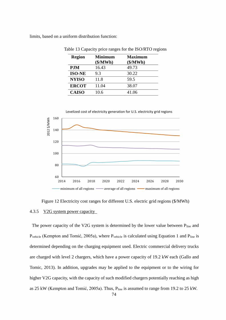
74

limits, based on a uniform distribution function:

Table 13 Capacity price ranges for the ISO/RTO regions

Region Minimum

($/MWh)

Maximum

($/MWh)

PJM 16.43 49.73

ISO-NE 9.3 30.22

NYISO 11.8 59.5

ERCOT 11.04 38.07

CAISO 10.6 41.06

Figure 12 Electricity cost ranges for different U.S. electric grid regions ($/MWh)

4.3.5 V2G system power capacity

The power capacity of the V2G system is determined by the lower value between Pline and

Pvehicle (Kempton and Tomić, 2005a), where Pvehicle is calculated using Equation 1 and Pline is

determined depending on the charging equipment used. Electric commercial delivery trucks

are charged with level 2 chargers, which have a power capacity of 19.2 kW each (Gallo and

Tomic, 2013). In addition, upgrades may be applied to the equipment or to the wiring for

higher V2G capacity, with the capacity of such modified chargers potentially reaching as high

as 25 kW (Kempton and Tomić, 2005a). Thus, Pline is assumed to range from 19.2 to 25 kW.

60

80

100

120

140

160

2014 2016 2018 2020 2022 2024 2026 2028 2030

20

12

$/M

Wh

Levelized cost of electricity generation for U.S. electricity grid regions

minimum of all regions average of all regions maximum of all regions

75

In conclusion, the EREV power capacity is limited by the vehicle, whereas the corresponding

BEV power capacity is limited by the charger, as the power capacity of the BEV exceeds the

maximum power capacity of its charging equipment.

4.3.6 Maintenance cost

Low maintenance costs are a major advantage of electric drive vehicles over traditional

vehicles, since the battery, motor and associated electronics all require little to no regular

maintenance. There are fewer fluids to change, brake wear is significantly reduced due to

regenerative braking features, and there are far fewer moving parts comparing to traditional

vehicles. For this study, the maintenance cost of diesel trucks is derived from a real-life test

(Lammert and Walkowicz, 2012), and is thusly assumed to have a triangular distribution

ranging from $0.11/mile to $0.16/mile. BEV maintenance costs are usually $0.06 cheaper per

mile than diesel maintenance costs (Gallo and Tomic, 2013), and EREV maintenance costs

are assumed to be $0.03 cheaper per mile than diesel maintenance costs. The maintenance

cost of the charging stations is assumed to be 10% of the initial equipment cost (Chang et al.,

2012).

4.3.7 Diesel price

Diesel fuel price projections in the five researched regions (U.S. Energy Information

Adiministration, 2015a) are used in this study to predict the fuel costs of diesel vehicles and

of EREVs. In addition, to cover all relevant uncertainties in these diesel price projections,

different case scenarios for high, low, and medium-level crude oil prices are considered.

Figure 4 shows the medium-oil-price diesel price projections as an example. It should be noted

that the price of diesel is measured in 2013 money, and is then converted to 2015 money to

ensure data consistency.

76

Figure 13 Diesel price projections in the researched ISO/RTO regions

4.3.8 Emission savings

Life Cycle Assessment is a well-established but still evolving method used to assess the

potential environmental impacts and/or resource consumption levels of a product or a process

throughout its entire life cycle, which is typically broken down into different phases as needed.

In this study, the GHG impacts of the following life-cycle phases will be emphatically

discussed to estimate the overall GHG emission savings of the V2G system: Gas turbine based

electricity generation and distribution (direct and indirect emissions), diesel upstream

production, downstream tailpipe emissions, and lithium-ion battery manufacturing.

The direct emissions of electricity are estimated using the reported emissions of power plants

in the GREET model (Argonne National Laboratory, 2013). These emissions are then

multiplied by the EIA’s electricity mix projections in the studied regions (U.S. Energy

Information Adiministration, 2015d) to estimate the regional direct emissions of electricity

generation. The indirect emissions of electricity, i.e. those associated with the transmission

and distribution of electricity, are estimated using the eGRID gross grid loss factors (U.S.

2.5

2.7

2.9

3.1

3.3

3.5

3.7

3.9

4.1

4.3

4.5

2016 2018 2020 2022 2024 2026 2028 2030

$ p

er G

allo

n

Diesel price projections (Medium Crude Oil Prices)

PJM CAISO ERCOT ISONE NYISO

77

Environmental Protection Agency, 2014b). Therefore, the indirect emissions and the

transmission losses from the purchase of electricity can be estimated using Equation 7 (Diem

and Quiroz, 2012). The eGRID database is used to compute the well-to-pump emission rates

of power plants, as shown in Equation 8. The GREET model (Argonne National Laboratory,

2013) and Hendrickson’s diesel tailpipe impact equation (Hendrickson et al., 2010) are used

to calculate the upstream and downstream GHG emissions, respectively, due to the production

and combustion of diesel fuel.

𝑈𝑝𝑠𝑡𝑟𝑒𝑎𝑚𝑘𝑗 =(𝑒𝐺𝑟𝑖𝑑)𝑘𝑗

(1−𝐺𝐺𝐿𝑗) (7)

Parameters:

𝑈𝑝𝑠𝑡𝑟𝑒𝑎𝑚𝑘𝑗: 𝑈𝑝𝑠𝑡𝑟𝑒𝑎𝑚 𝑎𝑚𝑜𝑢𝑛𝑡 𝑜𝑓 𝑎𝑖𝑟 𝑝𝑜𝑙𝑙𝑢𝑡𝑎𝑛𝑡 𝑘 𝑖𝑛 𝑟𝑒𝑔𝑖𝑜𝑛 𝑗 (𝑙𝑏/𝑘𝑊ℎ)

𝑒𝐺𝑟𝑖𝑑𝑘𝑗: 𝑒𝐺𝑟𝑖𝑑 𝑎𝑛𝑛𝑢𝑎𝑙 𝑒𝑚𝑖𝑠𝑠𝑖𝑜𝑛 𝑟𝑎𝑡𝑒 𝑖𝑛 𝑟𝑒𝑔𝑖𝑜𝑛 𝑗 𝑓𝑜𝑟 𝑎𝑖𝑟 𝑝𝑜𝑙𝑙𝑢𝑡𝑎𝑛𝑡 𝑘 (𝑙𝑏/𝑘𝑊ℎ)

𝐺𝐺𝐿𝑗: 𝑒𝐺𝑟𝑖𝑑 𝑔𝑟𝑖𝑑 𝑙𝑜𝑠𝑠 𝑓𝑎𝑐𝑡𝑜𝑟 𝑓𝑜𝑟 𝑟𝑒𝑔𝑖𝑜𝑛 𝑗Indexes:

𝑘: 𝑎𝑖𝑟 𝑝𝑜𝑙𝑙𝑢𝑡𝑎𝑛𝑡 𝑖𝑛𝑑𝑒𝑥 𝑓𝑜𝑟 𝐺𝐻𝐺

𝑗: 𝑟𝑒𝑔𝑖𝑜𝑛 𝑖𝑛𝑑𝑒𝑥

𝑈𝑝𝑠𝑡𝑟𝑒𝑎𝑚𝑘𝑗𝑦 = ∑ (𝑊𝑇𝑃)𝑘𝑝𝑝 × (𝐸𝑛𝑒𝑟𝑔𝑦𝑀𝑖𝑥)𝑝𝑗𝑦 ( 8 )

Parameters:

𝑈𝑝𝑠𝑡𝑟𝑒𝑎𝑚𝑘𝑗𝑦: 𝑈𝑝𝑠𝑡𝑟𝑒𝑎𝑚 𝑎𝑚𝑜𝑢𝑛𝑡 𝑜𝑓 𝑎𝑖𝑟 𝑝𝑜𝑙𝑙𝑢𝑡𝑎𝑛𝑡 𝑘, 𝑖𝑛 𝑟𝑒𝑔𝑖𝑜𝑛 𝑗, 𝑓𝑜𝑟 𝑦𝑒𝑎𝑟 𝑦 (𝑙𝑏

/𝑘𝑊ℎ)

𝑊𝑇𝑃𝑘𝑝: 𝑊𝑒𝑙𝑙 𝑡𝑜 𝑝𝑢𝑚𝑝 𝑎𝑖𝑟 𝑝𝑜𝑙𝑙𝑢𝑡𝑎𝑛𝑡𝑠 𝑜𝑓 𝑝𝑜𝑤𝑒𝑟 𝑝𝑙𝑎𝑛𝑡 𝑝 (𝑙𝑏/𝑘𝑊ℎ)

𝐸𝑛𝑒𝑟𝑔𝑦𝑀𝑖𝑥𝑝𝑗𝑦: 𝑝𝑜𝑤𝑒𝑟 𝑠𝑜𝑢𝑟𝑐𝑒 𝑝, 𝑖𝑛 𝑟𝑒𝑔𝑖𝑜𝑛 𝑗, 𝑓𝑜𝑟 𝑦𝑒𝑎𝑟 𝑦

Indexes:

78

𝑘: 𝑎𝑖𝑟 𝑝𝑜𝑙𝑙𝑢𝑡𝑎𝑛𝑡 𝑖𝑛𝑑𝑒𝑥 𝑓𝑜𝑟 𝐺𝐻𝐺


𝑦: 𝑦𝑒𝑎𝑟 𝑖𝑛𝑑𝑒𝑥

𝑝: 𝑝𝑜𝑤𝑒𝑟 𝑝𝑙𝑎𝑛𝑡 𝑖𝑛𝑑𝑒𝑥

Therefore the emissions savings of V2G for the regulation service can be estimated using

the following formula:

𝐸𝑚𝑖𝑠𝑎𝑣𝑖𝑛𝑔 = 𝐸𝑑𝑖𝑠𝑝 × 𝐸𝑚𝑖𝑡𝑟𝑎𝑑𝑖𝑡𝑖𝑜𝑛𝑎𝑙 − (𝐸𝑑𝑖𝑠𝑝 × 𝐸𝑚𝑖𝑔𝑟𝑖𝑑 + 𝐸𝑚𝑖𝑏𝑎𝑡𝑡𝑒𝑟𝑦 𝑤𝑒𝑎𝑟 𝑜𝑢𝑡) ( 9 )

Where 𝐸𝑑𝑖𝑠𝑝 is the dispatched electricity in kWh, , 𝐸𝑚𝑖𝑔𝑟𝑖𝑑 is the emissions rate of the

electricity generated by the grid mix in the studied region, and 𝐸𝑚𝑖𝑏𝑎𝑡𝑡𝑒𝑟𝑦 𝑤𝑒𝑎𝑟 𝑜𝑢𝑡 is the

emissions due to the battery wear-out from providing V2G services. It should be noted that

the gas turbine generator as a regulation service method has relatively low efficiency due to

the randomly ramp up/down of the power, and in fact it has been argued in the literature that

the efficiency of energy storage is two to three times as much as that of gas turbine generators

(Makarov et al., 2012). Therefore, in order to calculate the emission savings, 𝐸𝑚𝑖𝑡𝑟𝑎𝑑𝑖𝑡𝑖𝑜𝑛𝑎𝑙

is assumed here to be two to three times that of the stated gas turbine generator emission rate.

The GREET, EPA and EIA regional electricity generating emission rates are also used to

calculate emission savings. Moreover, in order to account for an additional level of uncertainty

in these values, it has been assumed that they each range within ±10% of their respective

projected values. The battery life cycle emissions were estimated using the EPA’s report on

EV lithium-ion batteries (Amarakoon et al., 2013), and the battery-related emissions for the

material extraction, manufacturing, use, and end-of-life phase are all considered.

79

4.3.9 Net revenue

The net revenue of V2G regulation services is calculated by subtracting the total cost from

the total revenue. Regulation service revenue depends on the market of the electricity that is

sold to. The previously developed methodology by Kempton and Tomic (Kempton and Tomić,

2005a) is mostly used to estimate the net revenue of V2G regulation services. However, in

order to account for uncertainty, different contributions are added to the existing methodology.

Thus, the total revenue to a regulation service provider consists of two separate revenue types:

capacity payments and energy payments.

Capacity payments are given for the availability of the power plugged in, and are measured

based on the contracted power capacity and the time the EV is plugged. Capacity payments

are calculated using Equation 5 below:

𝑅1 = 𝑃𝑟𝑖𝑐𝑒𝑐𝑎𝑝𝑃𝑑𝑖𝑠𝑝𝑇𝑝𝑙𝑢𝑔 (10)

Where R1 is the total capacity payment revenue, Pricecap is the regulation capacity price in

$/kWh, Pdisp the contracted available power in kW, and Tplug is the total vehicle plug-in time

in hours. The Pricecap is estimated based on the historical data of each ISO/RTO region

individually, and the regulation up and regulation down prices are assumed to be the same.

Pdisp is the smaller value between the power output of the vehicle and the maximum power

capacity of the charging infrastructure.

Energy payments, on the other hand, are given for the actual exchanged electricity via

regulation signal responses. Energy payment calculations are summarized in Equations 6 and

7:

𝑅2 = 𝑃𝑟𝑖𝑐𝑒𝑒𝑙𝑒𝐸𝑑𝑖𝑠𝑝 (11)

𝐸𝑑𝑖𝑠𝑝 = ∑ 𝑃𝑑𝑖𝑠𝑝 ×𝑁𝑑𝑖𝑠𝑝

𝑖=1𝑇𝑐𝑦𝑐 (12)

80

Where R2 is the total energy payment revenue, Priceele is the retail electricity price in $/kWh

as derived from the authors’ previous study (Noori et al., 2015), Edisp is the total dispatched

electricity in kWh, Ndisp the number of dispatches (regulation cycles), Pdisp is the requested

dispatched power in each regulation cycle in kW, and Tcyc is the actual time of one regulation

cycle in hours. The number of accepted regulation requests (Ndisp) is assumed to be uniformly

distributed from 30 to 40. Due to the random nature of regulation requests, the value of Tcyc

is randomly selected between 3.6 minutes and 9 minutes (Kempton et al., 2008). The annual

exchanged electricity is taken by summing all the random daily exchanged electricity during

365 days of the year. This process is performed for 1000 replications for each year, meaning

the analysis covers 1000 * 365 days combinations.

In summary, the total V2G regulation service net revenue is the sum of R1 (capacity

payments), R2 (energy payments) and deducted by C (the battery degradation) as calculated

in Equation 8.

𝑅 = 𝑅1 + 𝑅2 - C (13)

Regulation service costs (excluding operation or maintenance costs due to regular vehicle

usage) consist mainly of costs related to battery wear-out. The general formula for cost is

expressed as follows:

𝐶 =𝐶𝑏𝑎𝑡

𝐿𝑒𝑡𝐸𝑑𝑖𝑠𝑝 + 𝐶𝑎𝑐 (14)

Where C is the total regulation service cost, Cbat is the capital cost of the battery in $, Let is

the lifetime throughput energy in kWh, Edisp is the total dispatched electricity in kWh, and Cac

is the annualized capital cost in $. Cbat and Let are calculated as shown in Equations 10 through

12 below.

𝐶𝑏𝑎𝑡 = 𝐵𝑐𝑎𝑝𝑃𝑏𝑎𝑡 (15)

81

𝐿𝑒𝑡 = 𝐿𝑐𝐵𝑐𝑎𝑝𝐷𝑜𝐷 ( 1 6 )

𝐶𝑎𝑐 =𝐶𝑏𝑎𝑡

𝐿𝑒𝑡𝐸𝑑𝑖𝑠𝑝 ×

𝑑

1−(1+𝑑)−𝑛 (17)

Where Bcap is the battery capacity, Pbat is the battery unit price in $/kWh (Gallo and Tomic,

2013), Lc is the battery lifetime, DoD is the depth of discharge (which affects the overall

battery life), d is the discount rate, and n is the number of the year the battery will be used.

The aforementioned costs and revenues pertain solely to regulation services. The overall

cash flow, the capital costs of the vehicle and of the charging facility (excluding taxes and

licensing fees), and the operational costs (e.g. maintenance costs and fuel costs) in each year

are also included, as shown in Equations 13 and 14 below.

𝐴𝐶𝐹𝑣𝑗𝑦 = 𝑃𝑢𝑟𝑣 + 𝐸𝑞𝑢𝑖𝑝𝑦 + 𝐶ℎ𝑦 + 𝐸𝑙𝑒𝑗𝑦 − 𝑅𝑣𝑗𝑦 + 𝑉𝑀𝑣𝑦 + 𝐶ℎ𝑀 𝑦 + 𝐵𝑅𝑒𝑝𝑙𝑣𝑦 − 𝑆𝑎𝑙𝑣 ( 1 8 )

𝑁𝑒𝑡 𝑃𝑟𝑒𝑠𝑒𝑛𝑡 𝐴𝐶𝐹𝑣𝑗𝑦 = 𝐴𝐶𝐹𝑣𝑗𝑦

(1+𝑖)𝑦 (19)

Indexes:

𝑣: 𝑣𝑒ℎ𝑖𝑐𝑙𝑒 𝑡𝑦𝑝𝑒 𝑖𝑛𝑑𝑒𝑥


𝑦: 𝑦𝑒𝑎𝑟 𝑖𝑛𝑑𝑒𝑥

Where ACF is the annual cash flow, Pur is the vehicle purchasing cost, Equip is the

equipment upgrade cost, Ch is the charging station cost, Ele is the electricity cost, R is the

total V2G regulation service revenue, VM is the vehicle maintenance cost, ChM is the

charging station maintenance cost, BRepl is the battery replacement cost, Sal is the vehicle

salvage value, and i is the discount rate. Among the relevant cost categories, purchasing costs

for vehicles and for charging equipment purchasing are all added to the first year only, while

vehicle salvage revenue applies are added only to the end of the life cycle. All other cost

82

categories will be calculated and added to the total cost for each year.

The cost of a battery electric truck is three times as much as that of a diesel truck, and the

capital cost is often a significant hurdle for potential EV owners. To promote the adoption of

hybrid vehicles, plug-in electric vehicles, and related charging infrastructure, the federal

government and about 40 state governments currently provide a variety of incentives,

including income tax exemption, free parking, free registration, and free high-occupancy

vehicle (HOV) lane access (National Cpnference of state Legislatures, 2015). In most states,

the rebate or tax exemption for hybrid or electric cars can vary from $1,000 to $4,000.

However, for electric delivery trucks, which have very expensive initial costs, the State of

New York and the State of California currently provide a “first come first serve” fund to

compensate battery electric truck owners for as much as $60,000 per vehicle and $50,000 per

vehicle, respectively. Since not every state provides incentives for electric trucks or even for

electric cars, the applicable federal and state-level electric truck incentives have also been

taken into consideration for the studied regions. Table 14 shows the amount of incentives for

hybrid and battery electric trucks in the representative states of each ISO/RTO region.

Table 14 Federal and state electric truck incentives in the researched regions

Representative

States

PHEV (EREV) BEV

Federal Level - $4,000 (Jin et al., 2014) $7,500 (Jin et al., 2014)

PJM PA, WA, VA, DC,

NJ

$2,000 (Jin et al., 2014) $2,000 (Jin et al., 2014)

CAISO CA $1,500 (Wood, 2015) $50,000 (California

HVIP, 2015)

ERCOT TX $2,500 (National

Cpnference of state

Legislatures, 2015)

$2,500 (National

Cpnference of state

Legislatures, 2015)

ISONE ME, NH $0 (Jin et al., 2014) $0 (Jin et al., 2014)

NYISO NY $0 (U.S. Department of

Energy, 2015)

$60,000 (Truck

Voucher Incentive

Program, 2015)

83

4.4 Results

4.4.1 Cumulative costs of ownership and V2G regulation service net revenues of the BEV

and the EREV

Although the first cost of an electric drive vehicle normally serves as an economic

disincentive (which is even more significant for electric trucks), it is crucial to consider the

total ownership cost of a vehicle throughout its entire lifetime instead of only considering the

initial cost. Figures 14a through 14e depict the yearly cumulative ownership cost of the BEV

in the five researched ISO/RTO regions. As noted in the previous sections, in order to account

for uncertainty, ranges of key parameters are inputted to the developed model consisted by

equations in the method section. The model is then run for 1,000 replications, during each run,

random values within the preset ranges are selected for calculation. The ownership cost results

are then presented based on scenarios for the lowest, highest, and average values. Moreover,

the V2G implementation scenario (V2G) and the business-as-usual scenario without V2G

services (No-V2G BAU) are compared in each figure to indicate the potential benefits of V2G

services in each region. Overall, the cumulative cash flow in all five regions are incremental.

The lines indicating average cash flow grow steadily and slowly, while the corresponding

upper-range lines show two sharp increasing trends in the year 2021 and in the year 2026;

both of these years correspond with time points at which batteries were replaced, and thus a

relatively larger expenditure is added accordingly. On the other hand, the lower-range lines

indicate that battery degradation, daily usage, maintenance costs, and other cost-related

factors are minimal, and thus only one extra battery is needed throughout the vehicle’s lifetime.

At the end of the research period, the slight decline of the total cost is due to a one-time inflow

of revenue from the salvage of the vehicle. In the PJM, ISO-NE, and ERCOT regions, the

average net present values of the total ownership cost are approximately $320,000. However,

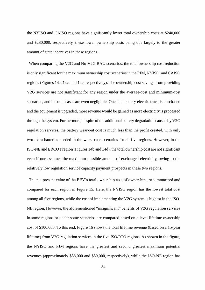
84

the NYISO and CAISO regions have significantly lower total ownership costs at $240,000

and $280,000, respectively, these lower ownership costs being due largely to the greater

amount of state incentives in these regions.

When comparing the V2G and No-V2G BAU scenarios, the total ownership cost reduction

is only significant for the maximum ownership cost scenarios in the PJM, NYISO, and CAISO

regions (Figures 14a, 14c, and 14e, respectively). The ownership cost savings from providing

V2G services are not significant for any region under the average-cost and minimum-cost

scenarios, and in some cases are even negligible. Once the battery electric truck is purchased

and the equipment is upgraded, more revenue would be gained as more electricity is processed

through the system. Furthermore, in spite of the additional battery degradation caused by V2G

regulation services, the battery wear-out cost is much less than the profit created, with only

two extra batteries needed in the worst-case scenarios for all five regions. However, in the

ISO-NE and ERCOT region (Figures 14b and 14d), the total ownership cost are not significant

even if one assumes the maximum possible amount of exchanged electricity, owing to the

relatively low regulation service capacity payment prospects in these two regions.

The net present value of the BEV’s total ownership cost of ownership are summarized and

compared for each region in Figure 15. Here, the NYISO region has the lowest total cost

among all five regions, while the cost of implementing the V2G system is highest in the ISO-

NE region. However, the aforementioned “insignificant” benefits of V2G regulation services

in some regions or under some scenarios are compared based on a level lifetime ownership

cost of $100,000. To this end, Figure 16 shows the total lifetime revenue (based on a 15-year

lifetime) from V2G regulation services in the five ISO/RTO regions. As shown in the figure,

the NYISO and PJM regions have the greatest and second greatest maximum potential

revenues (approximately $58,000 and $50,000, respectively), while the ISO-NE region has

85

the smallest maximum revenue. In addition, from the large whisker ranges in Figure 16, it can

be concluded that the V2G net revenue not only varies among the regions, but also changes

within each individual region depending on the amount of electricity exchanged through the

system.

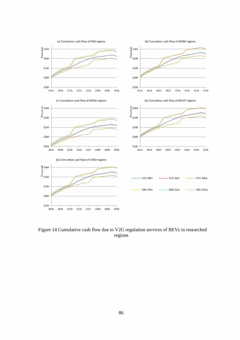
86

Figure 14 Cumulative cash flow due to V2G regulation services of BEVs in researched

regions

87

Figure 15 Net present value of BEV cost of ownership in researched regions

Figure 16 Total revenue of BEV-V2G services in researched regions

Figures 17a through 17e depict the yearly cumulative total ownership cost of the EREV,

which has similar upper-level, lower-level, and average cash flow trend as the BEV, but since

the initial cost of an EREV is typically lower than that of a BEV, the net present value of the

$200

$240

$280

$320

$360

$400

PJM ISO-NE NYISO ERCOT CAISO

Tho

usa

nd

sNet present value of BEV total cost of ownership (V2G provision)

$0

$10

$20

$30

$40

$50

$60

$70


Tho

usa

nd

s

Total revenue of BEV-V2G regulation services

88

lifetime ownership cost is also lower, now ranging between $210,000 and $230,000 for all

five ISO/RTO regions; this is also shown in Figure 18. According to the results, the total

ownership cost savings from providing V2G regulation services are only significant in the

NYISO and PJM regions (Figures 17a and 17c). Moreover, the battery replacement costs are

still differentiated from the normal ownership cost increasing trend, but the resulting costs are

still lower for EREV batteries than for BEV batteries because the battery capacity of the

EREV is only 50% as much as that of the BEV. Meanwhile, there is no large fund for hybrid

trucks among state governments, so the spatial ownership cost variations for the EREV are

not as significant as those for the BEV.

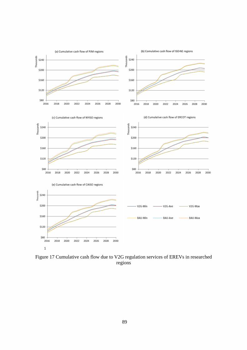
89

Figure 17 Cumulative cash flow due to V2G regulation services of EREVs in researched

regions

90

Figure 18 Net present value of EREV cost of ownership in researched regions

The net present value of the lifetime EREV V2G regulation service revenue is presented in

Figure 10. These total revenues for each region are less than their corresponding values for

the BEV because of the lower Pvehicle results, which in turn are due to the EREV having a

lower battery capacity than the BEV. However, based on the revenue results, EREVs can still

be an affordable and viable option as V2G service providers.

$160

$180

$200

$220

$240


Tho

usa

nd

s

Net present value of EREV total cost of ownership (V2G provision)

91

Figure 19 Total revenue of EREV-V2G services in researched regions

The diesel truck, as a reference case, has no accessibility to the grid and operates as a normal

commercial delivery truck. As shown in Figure 11, although diesel fuel prices have been

projected to vary in different regions, the total ownership costs of diesel trucks are identical

from region to region, with only a slightly higher level of uncertainty evident for the NYISO

region. That said, in spite of the much lower purchasing price of diesel trucks compared to

EREVs, the net present values of diesel truck total ownership costs are almost the same (or

higher in the PJM and NYISO regions) as those of the EREV (Figure 8f). This is because,

although traditional diesel trucks have lower initial costs, their long-term maintenance and

fuel costs can still add up to a relatively large sum of money.

As previously noted, a delivery truck fleet of 20 to 30 electric trucks is technically feasible

for bidding an ancillary service contract, and recently, the minimum capacity requirement for

ancillary service contracts have been lowered from 1MW to 100kW (Morash, 2013), meaning

that delivery truck fleets consist of electric trucks are now more applicable to provide ancillary

services. According to Figure 16 and 19, the equipment upgrade cost for V2G services

$0

$5

$10

$15

$20

$25

$30

$35

$40

$45


Tho

usa

nd

s

Total revenue of EREV-V2G services

92

(approximately $2,000) is considerably lower comparing to the overall V2G service revenues,

and the initial upgrading cost can be easily returned within a few years. In addition, due to the

excellent predictability of parcel delivery operations, idled electric trucks can be plugged to

the grid through the coordination of a dispatching center and serve as reliable ancillary service

providers.

4.4.2 GHG emission savings from providing V2G regulation services

Since the regulation service signals are random, there is no clear pattern of how much

electricity is exchanged through the V2G system, the calculation of electricity exchanging

follows a published work (Noori et al., 2016); as previously noted, a normal distribution

function has been applied to simulate regulation service request. A possible example of yearly

and 15-year cumulative GHG emission savings from providing V2G services is shown in

Figures 20 and 21. It should be noted that the V2G GHG emission savings presented here do

not include the life cycle emissions from regular vehicle operation.

Figure 20, as an example scenario of possible cumulative GHG emission savings, represents

the emissions saved from using BEVs as V2G regulation providers in the PJM region. The

emission savings in other regions have similar patterns, and therefore need not be explained

in any further detail.

93

Figure 20 Life-time GHG emission saving of BEVs in PJM regions

Figure 21 shows the cumulative GHG savings of V2G regulation services in the five

researched regions. From this figure, by plugging an idled BEV or EREV into the grid for

V2G regulation services, a single vehicle is able to save as many as 200 to 500 tons of CO2

over the entire 15-year lifetime of the fleet. In light of variations in the grid mixes (electricity

source distributions) of each region, the ISO-NE region yields the most emission savings

among all five regions, while NYISO region has the lowest emission savings. It can also be

concluded from the figure that, in spite of the higher battery capacity and output power of a

BEV as opposed to an EREV, BEVs do not necessarily yield more GHG emission savings

than EREVs, as the total exchanged electricity amount is limited based on the amount of

power requested by the grid operator rather than the power output of the vehicle; in other

words, despite the relatively lower battery capacity (40kWh) of EREVs, the EREV’s capacity

is still sufficient to meet the relevant V2G regulation service requirements.

0

100

200

300

400

500

2016 2018 2020 2022 2024 2026 2028 2030

CO

2(t

on

)

Cumulative GHG emission savings of BEVs in PJM regions

min avregae max

94

Figure 21 Cumulative GHG emission savings in the researched regions

4.4.3 Comparison of life cycle GHG emissions

In order to comprehensively evaluate the environmental benefits of electric trucks as

electricity regulation service providers, a more thorough life cycle assessment including

upstream and downstream/tailpipe emission of electricity and diesel is conducted for this

study. Figure 22 compares the life cycle GHG emission impacts of BEVs, EREVs (after

payload adjustment), and diesel trucks for each of the five researched ISO/RTO regions. In

this figure, the negative values represent the business-as-usual life cycle GHG emissions of

the three vehicle types, without the use of the V2G system. BEVs have no tailpipe emissions,

and therefore have lower total emissions even when upstream and downstream electricity

generation and transmission impacts are taken into consideration, and so BEVs have the

lowest BAU GHG impacts in all regions. In addition, based on the GHG impact results alone,

the NYISO and CAISO are the two most environmentally suitable regions for electric truck

implementation because of the low GHG emission factors of their respective grid mixes.

EREVs technically have lower GHG emission impacts than BEVs because, instead of driving

0

100

200

300

400

500

600

BEV EREV BEV EREV BEV EREV BEV EREV BEV EREV


CO

2(T

on

)

Cumulative GHG savings of V2G regulation services

95

with the engine directly as conventional hybrid vehicles do, EREVs are equipped with much

a smaller engine that powers an electric motor in order to generate its electricity; however,

while the researched diesel truck and battery electric truck have identical payloads, the

payload of the EREV in this study is approximate 50% as much as that of the other two truck

types, and so the EREV emissions shown in Figure 22 have been adjusted by a payload factor

to ensure that all results are for the same overall payload. After adjusting for payload, the

emission results of EREVs indicate no obvious advantages over diesel trucks, but the

environmental advantages of EREVs become more apparent when V2G emission savings are

taken into consideration. Over the 15-year research period, the emission savings of BEVs and

EREVs exceed their respective life cycle emission impacts due to electricity consumption.

Hence, although a considerably larger investment is needed to incorporate BEVs and EREVs

into the current truck fleets, the long-term environmental benefits of integrating EVs with the

grid are significant in most regions. In fact, with the potential introduction of carbon taxes,

these emission savings have potential to yield their own economic benefits as well.

Figure 22 Average V2G emission savings and life cycle GHG emissions of vehicles in the

researched regions

-400

-200

0

200

400

BEV EREV Diesel BEV EREV Diesel BEV EREV Diesel BEV EREV Diesel BEV EREV Diesel


CO

2(T

on

)

Average V2G emission savings and life cycle GHG emissions after payload adjustment

V2G Emission Savings Life Cycle Emissions After Payload Adjustment

96

In order to demonstrate the potential economic value of GHG savings, a carbon tax

projection is used to simulate the total tax savings of replacing current diesel trucks with

battery electric trucks in the PJM region (Figure 23). These tax savings are computed by

multiplying a proposed yearly federal carbon tax rate (2016-2030 projection) (Center for

Climate and Energy Solutions, 2013) with the overall life cycle GHG emission savings, more

specifically comparing a battery electric truck that provides V2G regulation services to a

regular diesel truck. Since EVs providing V2G services are actually mitigating GHG from the

environment instead of emitting to the environment, and carbon taxes are projected to increase

in the future, the tax savings due to GHG emission reductions could add up to as much as

approximately $18,000 by the year 2030.

Figure 23 Cumulative carbon tax savings of battery electric trucks compared to diesel trucks

in PJM regions

$0

$4

$8

$12

$16

$20

2016 2018 2020 2022 2024 2026 2028 2030

Tho

usa

nd

s

Cumulative carbon tax savings of BEVs in PJM regions

Min Ave Max

97

5 THE ROLE OF VEHICLE-TO-GRID SYSTEMS IN WIND POWER

INTEGRATION

A partial work of this chapter has been submitted to the Journal of Energy Policy

The large-scale integration of wind power must be supported by regulation services, which

are normally provided using combustion turbines. These regulation services can also be

provided using vehicle-to-grid systems, which utilize idle electric vehicle batteries to store

/re-supply energy from/to the grid. As discussed in Section 2 through Section 4, government

or commercial fleets are able to unify enough power capacity from their electric vehicles for

the regulation service provision in the initial phase of vehicle-to-grid system. However, a large

number of electric vehicles is needed for a large-scale vehicle-to-grid network to be functional;

and the potential to trigger marginal electricity generation by introducing numerous electric

vehicles must also be taken into account. Therefore, an agent-based model is developed to

simulate the integration of wind power into the power grid, as well as the regulation services

provided by a vehicle-to-grid system, and then compare the resulting greenhouse gas emission

savings from supporting the increased integration of wind power to the additional greenhouse

gas emissions from the large-scale charging of electric vehicles. The results indicate that, by

supporting the newly integrated wind power through a vehicle-to-grid system, greenhouse gas

emissions can be effectively mitigated in most of the researched regions if electric vehicles

are sufficiently available to meet the regulation requirements from vehicle-to-grid systems.

5.1 Background Information and Literature Review

5.1.1 ISOs/RTOs and wind power projections

The geological boundary of this study is based on seven ISO/RTO regions (Federal Energy

98

Regulatory Commission, 2016), specifically the CAISO, ERCOT, SPP, MISO, NYISO, PJM

and ISONE regions. This is in part because the electric power exchange between the ISO and

RTO regions is negligible, with only a 1% net exchange in 2010 (U.S. EPA, 2011); in fact,

the inter-regional electricity exchange could potentially be beneficial, but is currently

constrained by the limitations of current high-capacity transmission infrastructure (Flynn,

2008). Furthermore, the majority of the regional wind power transmission in the U.S. (about

80% (Gonzales et al., 2008)) is controlled by these same ISOs/RTOs, and the wind power

capacity corresponding regulation requirements are separately managed by each grid operator.

Lastly, current onshore wind projects are typically located in regions of high wind quality,

particularly coastal and central areas (Flynn, 2008), which mostly overlap with the scope of

the aforementioned ISO/RTO regions.

Some of the researched regions represent single states (the CAISO, ERCOT, and NYISO

regions), while others cover several states (the SPP, MISO, PJM, and ISONE regions).

Therefore, the wind power capacity at the ISO/RTO level is calculated as the sum of the

capacities of all of the major states within each independent grid operator region, as

summarized in Table 15. According to the U.S. Department of Energy’s wind power report

(Wiser et al., 2015), 7.7 GW of wind power will be integrated to the entire grid each year from

2015 to 2020, and 12.1 GW of wind power will be added to the grid each year from 2021 to

2030. Since these incremental introductions of wind power to the power grid will be integrated

nationwide, the wind power projection of each ISO/RTO region must be weighted based on

its current wind power capacity, and the installed wind power capacities and wind power

projections in each region are summarized in Table 15. In particular, the wind power

projections (last two columns from the left in Table 15) will serve as the key parameters in

the wind projection simulation of the ABM model.

99

Table 15 Current wind power installation and wind power projection in ISO/RTO regions

ISO/RTO Model

Code

States 2015 Installed

Wind Power

(MW)

Capacity

Ranking

Wind

Project

No.

Projects

Under

Construction

Weight 2016-2020

Yearly

Projection

(MW)

2021-2030

Yearly

Projection

(MW)

CAISO Region 0 California 6,022 2 123 86 0.11 847 1,332

ERCOT Region 1 Texas 16,406 1 112 6,343 0.30 2,309 3,628

SPP Region 2

Nebraska 810 20 16 116

0.15 1,169 1,837 Kansas 3,167 6 26 871

Oklahoma 4,330 4 29 1,199

MISO Region 3

North Dakota 1,886 11 22 736

0.34 2,653 4,170

Minnesota 3,035 9 94 551

Wisconsin 648 22 18 0

Iowa 5,710 3 99 679

Illinois 3,842 5 46 250

Indiana 1,745 13 14 150

Michigan 1,531 14 23 30

Missouri 459 25 6 0

NYISO Region 4 New York 1,749 12 25 0 0.03 246 387

PJM Region 5

Ohio 435 26 30 259

0.05 354 557 West Virginia 583 23 5 0

Pennsylvania 1,340 16 24 0

Maryland 160 31 4 31

ISONE Region 6

Maine 465 24 12 423

0.02 121 191 Massachusetts 107 34 44 8

New

Hampshire 171 30 5 14

Vermont 119 33 8 0

100

5.1.2 Wind integration and its impacts

In general, power grids are designed to accommodate a certain level of fluctuation.

Nevertheless, the intermittency of wind power would be amplified significantly as substantial

amounts of wind power are being integrated into the current power system, especially if such

integration takes place in a relatively short time interval as previously explained. As a result,

the minute-to-minute fluctuations in the power grid will increase significantly, and additional

grid ancillary services will ultimately be required to balance the resulting increase in power

supply fluctuations (Parsons et al., 2006). For simplification purposes, this paper will focus

only on the impact of wind integration on regulation service demand.

Albadi and El-Saadany (2010) previously studied the relationship between wind power

adoption and the corresponding ancillary service demand, and two important conclusions

were drawn based on their research. Firstly, the cost of ancillary services increases

significantly as wind power penetration grows, meaning that the increased integration of wind

power could become economically inefficient once the grid allocation of wind power exceeds

a certain limit. Secondly, the adoption of fast-responding generation/storage systems will be

crucial to reducing the overall cost of wind power. A study conducted by Korchinski (2013)

likewise confirms that large amounts of backup capacity must be online to ensure a stable

power output from wind projects, and that in the event of low power demand compared to the

wind power output at the time, the wind energy that might otherwise be wasted (“wind

dumping”) could instead be stored for later use as needed.

5.1.3 Electric vehicle market penetration projection

Based on the ABM simulation results with respect to wind power integration, the

corresponding regulation requirements, and the degree of EV market penetration needed to

101

meet these requirements are all calculated in this study using the methodology discussed in

Section 5.1.3, and the required number of EVs is then compared to current EV projections;

the smaller of these two values is then taken as the number of available EVs that will actually

provide regulation services. The methodology for calculating EV market penetration is

obtained from previous studies by the authors of this paper, and is also briefly introduced in

this section.

The vehicle price, maintenance cost, refueling cost, environmental impacts, government

subsidies, and other attributes related to EVs and/or traditional vehicles are all factors that can

affect a potential buyer’s choice regarding vehicle type, and these factors can also change on

a temporal and spatial basis (e.g. variations in fuel prices, electricity prices, or federal/state

rebates for EVs). Hence, a previously developed agent-based model (Noori and Tatari, 2016)

is used to simulate the market penetration of EVs (including battery electric vehicles (BEVs).

To project the regional market penetration of EVs, firstly, vehicle attributes are first derived

from a previously developed Electric Vehicle Regional Optimizer (EVRO) (Noori et al., 2015)

with uncertainties taken into account as appropriate. Next, an agent-based model (including

customers, vehicles, and regions as agents) is developed to simulate EV market penetration

in the next 15 years. Finally, the Exploratory Modeling and Analysis (EMA) method is used

to evaluate the results of the agent-based model. Since BEVs and EREVs both have grid

accessibility and large-capacity batteries, the combined number of these plug-in EVs is used

as the number of potentially available EVs in this study, and the resulting market penetration

data is shown in Figure 24 below

102

Figure 24 Regional EV market penetration projections

5.1.4 Electric vehicle charging and marginal electricity

Based on the conclusions of the authors’ previous study (Section 5.2.4), with government

incentives playing a critical role, the market penetration of plug-in EVs may increase to as

much as 26% by the year 2030 (Noori and Tatari, 2016). Also, a large EV fleet will

undoubtedly be a crucial connection between the transportation and electricity sectors and a

vital part of a smart city system, but studies have also shown that the charging behaviors of

EV owners may trigger marginal electricity generation (Ma et al., 2012) and thereby offset

the GHG emission mitigation benefits of V2G systems (Siler-Evans et al., 2012). In one such

study, McCarthy and Yang (2010) argue that a large-scale EV fleet may require extra

electricity from low-efficient combustion turbines. A study conducted by Green et al. (2011)

has likewise confirmed that the massive adoption of EVs may impact the electric network,

and possible charging scenarios with respect to plug-in EVs and their subsequent load impacts

have also been analyzed in the available literature (Hadley, 2006). In order to provide V2G

services, EVs are usually connected to the grid at night, but as the number of EVs plugged

into the grid increases significantly, a greater amount of marginal electricity demand is created

0

500

1,000

1,500

2,000

2,500

3,000

3,500

4,000

4,500

2016 2017 2018 2019 2020 2021 2022 2023 2024 2025 2026 2027 2028 2029 2030

Tho

usa

nd

sProjection of plug-in electric vehicle market penetration

CAISO ERCOT SPP MISO NYISO PJM ISONE

103

as a result (Hittinger and Azevedo, 2015), whereas coal plants are commonly used as a

primary marginal electricity generation source in some areas. Zivin et al. (2014) argue that

the emissions due to EV charging may vary spatially because of the regional differences in

average and marginal energy mixes, and have compared the marginal electricity emission

rates of each ISO/RTO region. Similarly, Kintner-Meyer et al. (2007) analyzed the impacts of

EV charging on the power grid in 12 ISO/RTO sub-regions.

5.1.5 System boundary

There are extensive studies in the available literature that analyze the impacts of wind

integration, the possible contribution of a V2G system on a renewable power network, or the

environmental impact of a large-scale EV fleet, and the potential of wind power and EVs to

mitigate environmental emissions has also been studied extensively. However, the

incremental or marginal effects of adding large amounts of wind power and EVs to the power

grid have not yet been researched on a holistic basis. To this end, the innovation and also the

first step of this study is to estimate the additional regulation requirement from the rapid

growth of wind power capacity, and to calculate the EV fleet scale needed to meet this

regulation requirement using V2G regulation services. Secondly, although some ISO/RTO

regions have considerably high wind integration projections, and therefore higher demand for

V2G services and/or EVs, the corresponding EV projections in each region may not be high

enough to meet the demand. Hence, to compare the supply/demand relationship with respect

to EVs in a future V2G-renewable power system, the EV projections from the authors’

previous study are used here to represent the overall EV population, and this study will also

compare the additional emissions from the marginal charging of this EV population to the

GHG emission savings from the use of the available EVs to provide V2G regulation services.

The third innovation of this study is its consideration of regional variations; all of the key

104

factors in this study (wind power projections, EV projections, marginal emission rates, etc.)

may vary from region to region, and the V2G-wind power system must therefore be analyzed

separately for each of the seven considered regions. Another important novelty of this study

is the policy analyses to be conducted. For instance, the wind project aggregation level and

the actual V2G signal strength are both deterministic factors that can affect the regulation

requirement level; the willingness of EV owners to provide V2G services and the charging

behaviors of said EV owners could lead to different performance levels for a particular V2G-

wind power system in any given scenario. Because these factors may be subject to change in

reality, this study will use the agent-based model developed in this study to analyze different

scenarios representing various combinations of key factors. The system boundary and the key

elements of this model are all shown in Figure 25.

Figure 25 System boundary

5.2 Method

5.2.1 Agent-based modeling

Using AnyLogic software (Anylogic, 2015), an agent-based model is developed to evaluate

105

and analyze the mechanisms of the V2G-wind power system to be considered in this study.

The main agent in this model, which also functions as the basic modeling environment, is

defined as one of the researched ISO/RTO regions. Within this main agent, regional wind

power agents are introduced to represent the growth of wind power in the researched region

(Table 15). Each wind power agent represents 1 MW of increased wind power capacity. The

wind power is assumed to be zero at the start of the simulation (the beginning of 2016), since

this study will focus on the incremental increase of wind power capacity and its subsequent

impacts, and the wind power capacity will reach the projected amount (Table 15) by the end

of the simulation. The wind power agent also reflects the aggregation of wind projects, which

may increase grid stability and reduce regulation requirements. Based on estimated

assumptions regarding the regulation requirement rate, the regulation services required each

year are evaluated based on the population number of the wind power agent, thereby obtaining

the required number of EVs to meet the demand. The number of required EVs in each year is

then compared to the available number of EVs, which is simulated using a lookup function of

the EV market penetration projections as previously discussed. The model is designed to

select the smaller number of EV between these two values in each year, which is used to

represent the total available number of EVs for providing regulation services. Finally, the

model will calculate the overall emission savings in each year based on the model’s key

parameters (V2G signal data, combustion turbine emission rate, marginal electricity emission

rate, etc.). The aforementioned processes are then repeated six more times with different data

sets to cover the 15-year projections for each region. Each individual process in this

methodology is explained in further detail in the following sections, and the outline of this

methodology is also summarized visually in Figure 25.

106

5.2.2 Modeling of wind integration and aggregation

The regulation requirement of wind integration is ultimately due to the lag between the rapid

growth of wind capacity in the power grid and the completion of an inter-regional

cooperating/supporting system. The voltage or frequency of a local grid is inherently unstable

because of the random turning on/off of millions of appliances at any given time, as well as

the potential for the sudden failure of generators. The newly added wind capacity, due to its

inherently intermittent nature, inevitably increases the level of uncertainty or variability in its

host area.

Nevertheless, the corresponding regulation requirement may not always be linearly

correlated to the incremental wind capacity, because wind projects have been found to benefit

significantly from the aggregation of wind power (Kirby, 2005). One study (Kirby and Hirst,

2000) suggests that, when a large wind project has a capacity scale as large as its host area,

and the overall incremental increase in wind capacity is 41% instead of doubling the total

regulation requirement. Due to the complexity of such systems, there is currently no unified

standard or regulation available as a reference to quantify the benefits of wind aggregation,

but a study conducted by Kirby et al. (2012) has indicated that the optimized regulation

requirement could range from approximately 30% to 50% of the total “stand-alone” regulation

requirement of the wind projects in question, depending on the level of aggregation being

considered.

The detailed simulation of the development of a well-coordinated national wind aggregation

system is beyond the scope of this study. Instead, to represent this wind aggregation process

as simply as possible without compromising the accuracy of the model, the increasing process

of individual agents (each representing 1 MW of newly installed wind capacity) is divided

into three phases as shown by the state chart in Figure 3: low aggregation, medium

107

aggregation, and high aggregation. In other words, the increasing pattern and growth rate of

wind power agents follows the projections previously cited in Table 15 (last two columns

from the left). After the construction of the model, and at the beginning of the simulation, the

wind power agents enter the low-aggregation state first. The arrows on the left-hand side of

Figure 3 with a clock represent a “time out” function in Anylogic, meaning that the agents

stay in this state for a certain period of time and then enter the next state. The rates of the two

time out functions “AggregationPhase1” and “AggregationPhase2” are both assumed to be

five years, meaning that the newly added wind capacity is at a low aggregation state, or stand-

alone state, from 2015 to 2020, due to insufficient transmission infrastructure for higher

aggregation levels. Hirst and Hild (2004) found that the regulation requirement rate for wind

projects is 0.5%, while Hudson et al. (2001) argue that this rate could be as high as 6%; since

both rates have been confirmed in a separate study (Kempton and Tomić (2005b), the low

aggregation regulation requirement rate is assumed to be 6% on average, ranging from 2% to

9%. Similarly, the wind power agents shifting from a low aggregation state to a medium

aggregation state stay in the medium aggregation state for another five years, and then change

to high aggregation state through the time out function “AggregationPhase2”; the regulation

requirement rate in this state is assumed to range from 1% to 5%, with a default value of 3%.

It should be noted here the regulation requirement is reflected in the main agent and

subsequently used as one of the key parameters in later calculations. The arrows on the right

side of the state chart are used to simulate the wind aggregation process. The arrow within the

second state, “AggregationPotential1”, is a rate function (its rate being equal to the first-order

delay in stock and flow diagrams (Osgood, 2011)) that sends a message (“Aggregation”) to a

random agent in the last state (“LowAggregation”); whichever agent in the low aggregation

state receives this message has a certain probability to change to the medium aggregation state.

For purposes of this model, the rates “AggregationPotential1” and “AggregationWillingness”

108

are both assumed to be 0.5. The messaging and shifting process in this model simulates the

aggregation process: by the time agents accumulate in the medium aggregation state, based

on the infrastructure projections previously discussed, a preliminary network will have been

formed to some extent, and the current wind capacity and/or new wind projects will therefore

have a chance to reach out and connect to the capacity of currently “stand-alone” and/or low-

aggregation project, the probability of which is simulated in the rate “AggregationPotential1”.

When this chance emerges, it then becomes possible that the projects involved could

successfully integrate with each other and thus share the reduced regulation burden equally;

this probability is represented using “AggregationWillingness”, which is initially assumed to

have a value of 0.5. The values of these two rates are empirical, and may therefore change

accordingly during the policy tests to be conducted in this study. The aggregation process is

likewise repeated for agents shifting from medium aggregation to high aggregation, at which

point the agents will stay in a high-aggregation state for five years until 2030. During this

period, the highly aggregated wind power network could be supported with a relatively lower

regulation rate, which is thus assumed to range from 0.5% to 3%. The movement of the wind

power agent is shown in Figure 26.

109

Figure 26 State chart of wind aggregation in a typical wind power agent

5.2.3 Required number of EVs and projected EV market penetration levels

The total regulation requirement throughout the research period is obtained by multiplying

the total added wind capacity at each stage by the corresponding regulation requirement rate,

after which the calculated regulation requirement value is used as an input to calculate the

total number of required EVs.

The required number of EVs for a V2G regulation service contract can be calculated by

dividing the total regulation requirement by the average power output of an individual vehicle

providing V2G services (Hill et al., 2012). The power output, or available power, of each EV

is calculated using Equation 1, which has been developed in a previous study (Kempton and

Tomić (2005a). In addition, a battery agent is included in the model to reflect any potential

variations in the power output.

𝑃𝑣𝑒ℎ𝑖𝑐𝑙𝑒 =(𝐵𝑐𝑎𝑝 −

𝐷𝑣𝑚𝑡 −𝐷𝑏𝑢𝑓𝑓𝑒𝑟

𝐹𝑒 ) 𝐶𝑒

𝑇𝑑𝑖𝑠𝑝𝑎𝑡𝑐ℎ ( 2 0 )

110

Where Pvehicle is the total available power capacity in kW, and Bcap is the battery capacity of

the vehicle in kWh. The battery capacity of common EREVs, such as the Nissan Leaf S,

currently range from 20 kWh to 24 kWh (Nissan, 2015; Plugincars, 2015; Volkswagen, 2016).

However, accounting for the average battery capacity of the entire EV fleet, it is

conservatively assumed that the average EV battery capacity is initially 20 kWh in the year

2016 and then increases linearly to 26 kWh by the year 2030. Dvmt is the average daily vehicle

mileage travelled by personal cars, which is assumed to be 30 miles based on the available

literature (Statistic Brain Research Insititute, 2015; U.S. DOT, 2009), and Dbuffer is the range

that an EV driver would like to conserve as backup and/or to avoid range anxiety; this value

is usually 20 miles on average (Kurani et al., 1994), but since EREVs have gas as a backup

power source, and with the growing development of charging infrastructure, the buffering

range is assumed to drop from 20 miles to 16 miles over the 15-year simulation period,

meaning that the available power from the vehicle increases slightly over time. Fe is the fuel

efficiency of an EV in miles/kWh, which is assumed in this model to have an average value

of 3.5 based on available manufacturer data (Nissan, 2015; Plugincars, 2015). Ce is the

transmission efficiency of the transfer of electricity from the EV batteries to the power grid,

which is assumed to have a value of 0.93 (Sioshansi and Denholm, 2010). And finally, Tdispatch

is the accumulative regulation signal answering time (not the plug-in time) in hours, the value

of which is conservatively assumed to be 0.3 hours (18 minutes) (Kempton and Tomić, 2005a).

Accounting for all of the relevant assumptions and parameters as the model runs, the growth

pattern of EV output power over the course of the simulation period is presented in Figure 27,

where the y-axis of the graph is the power capacity in kW.

111

Figure 27 EV output power

The number of required EVs in each year is then calculated and compared to the number of

available EVs, the latter of which is calculated as shown in Equation 21 below:

𝑁𝑢𝑚𝑏𝑒𝑟 𝑜𝑓 𝐴𝑣𝑎𝑖𝑙𝑎𝑏𝑙𝑒 𝐸𝑉𝑠 = 𝐸𝑉𝑀𝑃𝑖𝑗 × 𝑊𝑟 × 𝐴𝑟 ( 2 1 )

Where EVMPij is the EV market penetration during year i in region j, Wr is the percentage

of EV owners who are willing to provide V2G services (assumed to be 0.05 on average, with

a range from 0.01 to 0.1), and Ar is the rate of availability with respect to V2G service

providers (assumed to be 0.3 on average, with a range from 0.1 to 0.5). The values and ranges

of both the willingness rate and the availability rate are derived from relevant studies in the

available literature (Kempton and Tomić, 2005b; Parsons et al., 2014), and these changeable

ranges will be necessary for testing different scenarios and/or policies as explained in more

detail in this study.

A separate algorithm is designed within the main agent to select the smaller value between

the number of required EVs and the number of available EVs, and the result of this algorithm

is taken as the actual number of EVs that will provide V2G services for the wind projects in

the model.

112

5.2.4 V2G emission savings and additional emissions from marginal generation

Most of the total grid ancillary service requirement is currently provided by flexible yet low-

efficiency combustion turbines, such as gas turbines or combined-cycle generators, and the

repeated ramping up/down of these generators may cause significantly more GHG emission

impacts compared to energy storage methods, so the GHG emission impacts of fossil fuel

combustion can be mitigated by replacing traditional combustion turbines with EV batteries

through the use of a V2G system. However, there is no data in the available literature

regarding regulation signals from wind intermittency, so the relevant parameters with respect

to V2G regulation signals are instead obtained from the available literature where available,

and are assigned ranges in this manner in order to explore the potential variations from the

implementation of different policy scenarios; a similar method has also been used in the

previous sections. V2G emission savings are calculated using Equation 3 below:

𝐸𝑆 = 𝐸𝑉𝑖𝑗 × 𝑃𝑐𝑦𝑐𝑙𝑒 × 𝑁𝑑𝑖𝑠𝑝𝑎𝑡𝑐ℎ × 𝑇𝑐𝑦𝑐𝑙𝑒 × 𝐸𝑚𝑖𝑠𝑠𝑖𝑜𝑛𝑐𝑡 × 𝐸𝑅 × 𝐸𝐿 × 365 ( 2 2 )

Where ES is the emission savings from the use of V2G regulation services, EVij is the actual

amount of EVs that can provide V2G services as previously calculated in Section 5.3.3, Pcycle

is the signal strength of each regulation request in MW (with an assumed default value of

0.0075 and an overall possible range from 0.001 to 0.01), Ndispatch is the number of regulation

cycles per night (which ranges from 30 to 40 with a median value of 35), and Tcycle is the time

interval of each regulation up/down request (which ranges from 0.06 to 0.15 hours, or 3.6 to

9 minutes). Pcycle, Ndispatch, and Tcycle are the key parameters that determine the amount of

exchanged electricity per vehicle per night, the values and ranges of which have all been

already well explained in previous sections; furthermore, these parameters’ values are

changed as appropriate for different scenarios. Emissionct is assumed to be equal to 0.567

tons/MWh, which is the GHG emission rate of gas turbines as previously published by the

113

Environmental Protection Agency (EPA). The parameter “ER” represents the higher

efficiency rate of energy storage means over traditional combustion turbines, the value of

which ER is assumed to be 2.5 based on previous studies from the available literature (Lin,

2011; Makarov et al., 2012). Finally, EL is the energy loss factor for battery

charging/discharging, the value of which is assumed to be 0.837 (Kempton et al., 2001).

On the other hand, the charging of a newly introduced large-scale EV fleet may add a considerable

burden to the grid; for example, in the worst-case scenario, if one million EVs were charged at the

same time, there would be a 6 GW surge on the grid (Zivin et al., 2014). Equation 4 below uses the

relevant parameters to calculate the additional emissions from marginal electricity generation.

AE = 𝐸𝑉𝑀𝑃𝑖𝑗 × 𝑁𝐶𝑅 ×𝑆𝑂𝐶𝑣𝑎𝑟

1000× 𝐵𝑐𝑎𝑝 ×

𝑀𝐸𝑚𝑖𝑠𝑠𝑖𝑜𝑛𝑗−𝐴𝐸𝑚𝑖𝑠𝑠𝑖𝑜𝑛𝑗

2000× 365 ( 2 3 )

Where AE is the additional GHG emissions in lb/MWh, NCR is the fraction of EVs that are

charged at night with marginal electricity (which ranges from 0.7 to 0.8 (Hittinger and

Azevedo, 2015)), SOCvar is the percentage variation of the battery’s state of charge (SOC),

and MEmissionj - AEmissionj represents the difference between the marginal emission rate

and the average grid mix emission rate in region j (Rothschild and Diem; U.S. Environmental

Protection Agency, 2015b). The detailed data resulting from these calculations is summarized

in Table 16

114

Table 16 Marginal and average emission rate of the researched regions

ISO/RTO Model

Code

eGRID Sub-region Electricity

Mix Average

Emission

Rate

(lb./MWh)

Non-baseload

Combustion

Plants

Emission Rate

(lb./MWh)

Average Mix

and Non-

baseload

Difference

(lb./MWh)

Annual

Generation

(MWh)

Weight Weighted

Emission

Rate

(lb./MWh)

CAISO Region 0 WECC California 652.72 956.36 303.64 206,633.04 1.00 303.64

ERCOT Region 1 ERCOT All 1,147.21 1,412.91 265.70 360,221.52 1.00 265.70

SPP Region 2 SPP North 1,730.49 2,133.66 403.17 69,447.96 0.31 235.20

SPP South 1,545.32 1,704.14 158.82 152,734.00 0.69

MISO Region 3 MRO East 1,531.00 1,971.54 440.53 28,629.06 0.05 599.17

MRO West 1,433.25 2,106.28 673.03 203,915.89 0.37

SERC Midwest 1,719.68 2,067.19 347.51 132,935.70 0.24

SERC Mississippi

Valley

1,056.65 1,410.46 353.81 182,134.13 0.33

NYISO Region 4 NPCC Long Island 1,205.90 1,206.44 0.55 12,121.64 0.09 521.04

NPCC

NYC/Westchester

698.08 1,109.82 411.74 45,503.84 0.32

NPCC Upstate NY 410.31 1,068.02 657.71 82,550.86 0.59

PJM Region 5 RFC East 862.68 1,504.24 641.56 262,972.20 0.29 543.69

RFC Michigan 1,577.34 1,811.01 233.66 86,819.39 0.09

RFC West 1,386.55 1,932.32 545.77 567,064.67 0.62

ISONE Region 6 NPCC New England 642.75 1,012.24 369.49 120,324.52 1.00 369.49

115

5.3 Results

The developed model is run to analyze the performance of the V2G-wind power system, and

the results are shown and explained in this section, including the projections and aggregations

of newly installed wind capacity, the regulation requirements in each of the ISO/RTO regions

due to increased wind power integration, comparisons of the number of EVs required to meet

the regulation requirement and the actual available number of EVs, and most importantly, the

overall emission savings performance of the modeled system under various realistic scenarios.

Figures 28a through Figure 28g depict the increasing market penetration and aggregation

levels of wind power in all seven ISO/RTO regions. The three layers of the overall wind power

capacity in one region represent the wind power projects that are stand-alone projects (low

aggregation), partially aggregated (medium aggregation) and fully aggregated (high

aggregation) with respect to their nearby wind power supply area (or host area), and the

increase in aggregation starts in the year 2020 and progress every five years afterward. As

shown in the figures, the MISO and ERCOT regions have the largest wind power projections,

the SPP and CAISO regions have relatively mid-level projections, and the projections in the

NYISO, PJM and ISONE regions are fairly small. The degree of wind power integration in

each region follows an identical pattern over time, but as the predicted 765 kV transmission

network is built within a 15-year interval, the later-incorporated and highly aggregated wind

power projects will require less regulation support and thereby decrease the overall regulation

requirement at the end of the simulation period. Also as shown in the figures, the medium-

aggregation and high-aggregation phases start in 2020 and in 2025 respectively, thus

validating the coding of the wind power agent.

In addition, as stated before, this study analyzes the performance of the V2G-wind power

system under different policies or scenarios, and five scenarios are tested within the model

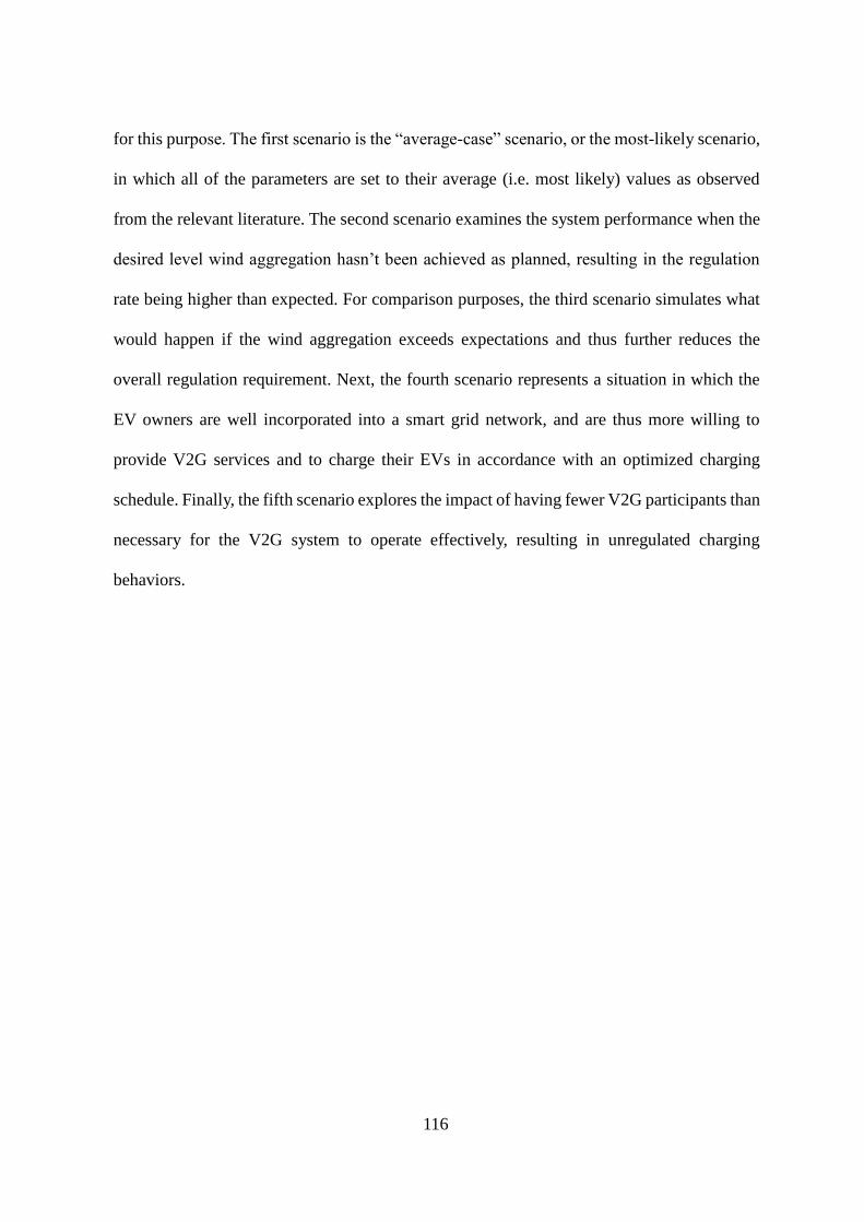
116

for this purpose. The first scenario is the “average-case” scenario, or the most-likely scenario,

in which all of the parameters are set to their average (i.e. most likely) values as observed

from the relevant literature. The second scenario examines the system performance when the

desired level wind aggregation hasn’t been achieved as planned, resulting in the regulation

rate being higher than expected. For comparison purposes, the third scenario simulates what

would happen if the wind aggregation exceeds expectations and thus further reduces the

overall regulation requirement. Next, the fourth scenario represents a situation in which the

EV owners are well incorporated into a smart grid network, and are thus more willing to

provide V2G services and to charge their EVs in accordance with an optimized charging

schedule. Finally, the fifth scenario explores the impact of having fewer V2G participants than

necessary for the V2G system to operate effectively, resulting in unregulated charging

behaviors.

117

Figure 28 Regional wind integration and aggregation (MW)

5.3.1 Average-case scenario

Under this scenario, the values of all of the key parameters within the model (regulation rate,

V2G signal strength, participation willingness, night charging ratio, etc.) are all set to their

most likely values as observed from the literature, meaning that the results of this scenario

a. CAISO b. ERCOT

c. SPP

d. MISO

e. NYISO

f. PJM

g. ISONE

118

reflect the most likely impacts of using V2G systems to support the increased adoption of

wind power in the power grid. Figure 6 indicates the regulation requirement projections in

each of the seven regions. As shown in this figure, the regulation requirement is positively

correlated with the wind power projection; for instance, the MISO and ERCOT regions have

the highest wind power projections and each require approximately 1,200 MW and 1,000 MW

in regulation services, respectively. Conversely, the regulation requirements in the SPP and

CAISO regions increase more gradually, and due to their lower wind integration projections,

the PJM, NYISO and ISONE regions all tend to have minimal regulation requirement levels.

Furthermore, the results shown in Figure 29 also validate the model. First, the growth rate of

the total regulation requirement is linear in the first five years due to the low aggregation

levels of wind projects at the time. Then, from 2020 to 2025, the growth rate of the overall

regulation requirement begins to take on a smoother pattern, and after 2025, the total

regulation requirement starts to decrease in most regions because the high level of aggregation

of wind power at that point ultimately reduces the variability of its output and thus reduces

the need for regulation services.

Figure 29 Regional projection of regulation requirement (Scenario 1)

0

200

400

600

800

1,000

1,200

1,400

2015 2016 2018 2019 2020 2021 2022 2023 2024 2025 2026 2027 2028 2029 2030

MW


119

The number of EVs needed to provide these regulation services is compared to the total

available number of EVs in each region, as shown in Figure 30a through Figure 30g. The

CAISO region has a relatively large EV market penetration projection, and although the total

EV population cannot provide the total required number of EVs in the first seven years of the

simulation period, the availability of V2G providers increases significantly after 2022.

Conversely, the lower EV projections in regions such as the ERCOT, SPP, MISO and NYISO

regions lack the potential to support a V2G system even though most of these regions have

considerably large wind power market penetration levels (thus requiring more EVs). On the

other hand, the in PJM region has the highest EV projection, but its need for V2G services is

relatively low. The ISONE region has the lowest available EV and required EV projections,

suggesting that the power and transportation structure in the ISONE region may remain

unchanged for the next 15 years.

120

a. CAISO

b. ERCOT

c. SPP

d. MISO

e. NYISO

f. PJM

g. ISONE


(Scenario 1)

The final and most important results (net overall GHG emission savings) are calculated by

subtracting the emission savings of the V2G system from the additional emissions due to the

consumption of marginal electricity, and the results are shown in Figure 31. Although the

CAISO region has a relatively mid-level wind power projection, it also yielded the most net

overall emission savings, mainly because the EV projection in the CAISO region is enough

121

to fully support the V2G-wind power system. Moreover, in spite of their higher wind

integration projections and emission saving potentials, the smaller EV populations in the

MISO and ERCOT regions ultimately limit their net GHG emission mitigation benefits.

Similarly, the emission savings goals of the V2G system in the PJM region are ultimately

achieved because of the PJM region’s future EV market penetration rates.

Figure 31 Overall GHG emission savings in researched regions (Scenario 1)

5.3.2 Low wind aggregation scenario and high wind aggregation scenario

In order to simulate a scenario in which the overall wind power aggregation level is less than

expected, the regulation requirement rates at each regulation level are set at their maximum

values prior to running the simulation and the three parameters related to V2G signal strength

related (Pcycle, Ndispatch and Tcycle) are also set at their maximum values. Figure 32 shows the

regulation requirement projections for each region in this scenario. The pattern and sequence

of the regulation requirements in the researched regions are identical to those of the average-

case scenario (Figure 29), the main difference being that the MISO, ERCOT, SPP and CAISO

regions each require about 200 MW of additional regulation capacity due to their low

aggregation levels. Additionally, as shown in Figure 33a through Figure 33g, the patterns of

0

20,000

40,000

60,000

80,000

100,000

120,000

140,000

160,000

2015 2016 2018 2019 2020 2021 2022 2023 2024 2025 2026 2027 2028 2029 2030

ton

GH

G


122

the required number of EVs and the available EV populations are also identical to those of

the average-case results in all regions, except for a slightly larger number of required EVs

since more V2G service capacity is needed due to the lack of aggregation, and it also takes

ten years for the CAISO region to meet (and later exceed) its EV requirements. It can likewise

be concluded from Figure 34 that, although the potential of V2G systems to save on GHG

emissions is limited in most regions due to the low availability of EVs, the overall GHG

emission savings are still two to three times as much as those of the average-case scenario,

primarily due to the V2G regulation signal strength. Since the aggregation level of the new

wind capacity is low, the use of independently operated wind projects introduces more

variability (and thus instability) to the power grid, meaning that more electricity is exchanged

during V2G operation, and the overall GHG emission savings are increased as a result.


0

200

400

600

800

1000

1200

1400

1600

1800

2000

2015 2016 2018 2019 2020 2021 2022 2023 2024 2025 2026 2027 2028 2029 2030

MW


123

a. CAISO

b. ERCOT

c. SPP

d. MISO

e. NYISO

f. PJM

g. ISONE


(Scenario 2)

124


Unlike the low wind aggregation scenario, an optimal scenario assuming the achievement of

a higher level of wind aggregation than expected due to the completion of regional

transmission networks and the cooperation of local grid operators. To simulate this scenario,

the regulation rates of each aggregation level are set at their minimum values. A highly

aggregated wind power network is also introduced into the model to mitigate the fluctuations

associated with wind intermittency, and the V2G signal strength is therefore set at its

minimum value as well. The resulting regulation requirement projections are presented in

Figure 35. Once again, the pattern and sequence are similar to the results of the formal two

scenarios, except that now the required regulation service capacities are much lower than

those of the average-case scenario. However, due to the significantly reduced regulation

requirements, fewer EVs are required, and the required number of EVs in each region is less

than the corresponding number of available EVs in most of the studied regions (Figure 36a

through Figure 36g), except in the ERCOT, SPP and MISO regions, where the wind power

projections are still much higher than in the average-case scenario. Figure 37 depicts the

0

50,000

100,000

150,000

200,000

250,000

300,000

350,000

400,000

450,000

500,000

2015 2016 2018 2019 2020 2021 2022 2023 2024 2025 2026 2027 2028 2029 2030

ton

GH

G


125

overall GHG emission savings based on these assumptions, and as shown in this figure, the

resulting emission savings are shown to be much lower than those of the average-case

scenario. The ERCOT and MISO regions have the largest amount of emission savings,

because although the required number of EVs in each of these two regions is still larger than

the number of available EVs, the difference between the two is considerably small (Figure

36b and Figure 36d), meaning that the V2G emission savings potential is still well utilized

because the available EV population is still relatively sufficient comparing to the required

number of EVs. Furthermore, the wind power projections in these two regions are higher, and

more emissions can therefore be saved through the use of a V2G system. Lastly, the

availability of EVs in the CAISO region is still better than those of other regions, but in this

scenario, the reduced wind power projections is a major limitation in terms of GHG emission

mitigation. It should be noted in this regard that the emission savings in the ISONE region is

shown to have a negative value, because the V2G regulation requirement is fairly low and

thus only a very small amount of GHG emissions can be saved through the use of a V2G

system in this region, while the newly adopted EVs consume a significant amount of marginal

electricity and results in a net increase in GHG emissions, hence the negative result.

By comparing Figures 33 and 36 to Figure 30, it can be concluded that, as the regulation

requirement rate increases, the required number of EVs for regulation services in all regions

also increases, and vice versa. Moreover, the amount of required EVs is positively correlated

with the scale of incremental wind power installation in each region. Altogether, these

relationships validate the mathematical structure of the model developed for this study.

126


0

50

100

150

200

250

300

350

400

450

2015 2016 2018 2019 2020 2021 2022 2023 2024 2025 2026 2027 2028 2029 2030

MW


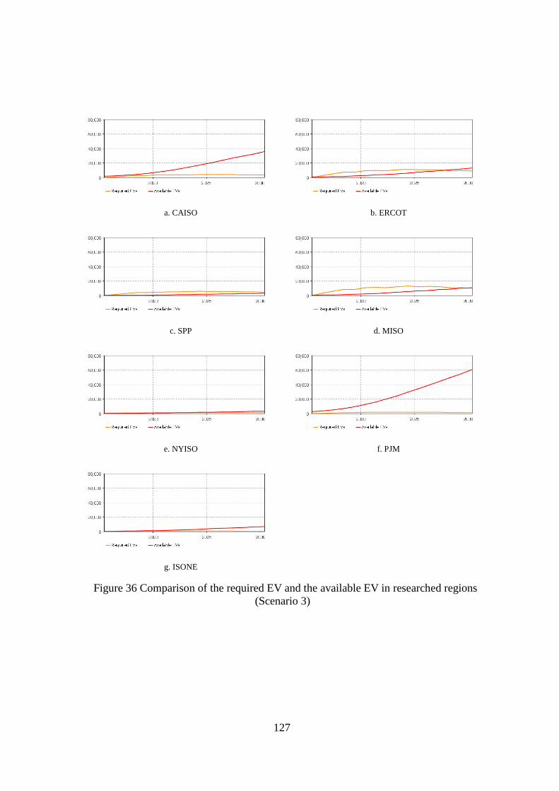
127

a. CAISO

b. ERCOT

c. SPP

d. MISO

e. NYISO

f. PJM

g. ISONE


(Scenario 3)

128


5.3.3 High participation/regulated charging scenario & low participation/unregulated

charging scenario

From a V2G service provider’s perspective, the willingness of EV owners to provide

regulation services is a deterministic factor that directly affects the availability of EVs for the

V2G-wind power system, and EVs, as a basic and crucial element in a smart grid and/or smart

city system, can not only function as stabilizers, but can also operate on an optimized schedule.

Therefore, in a sophisticated EV network, the V2G service participation ratio is high, and

more EVs are charged at ideal times to maximize environmental and economic benefits. To

simulate this scenario, the willingness and availability of EV owners to provide V2G services

are each set at their maximum values, while the night charging ratio and SOC variations are

each set at their minimum values. The regulation requirement projections in this scenario are

the same as those of the average-case scenario because both scenarios reflect the uncertainties

from the V2G service supplier’s perspective. Figure 38a through Figure 38g illustrate the

comparison between the number of available EVs and the number of required EVs in each

-5,000

0

5,000

10,000

15,000

20,000

25,000

30,000

35,000

2015 2016 2018 2019 2020 2021 2022 2023 2024 2025 2026 2027 2028 2029 2030

ton

GH

G


129

region. The overall number of available EVs increases significantly in this scenario, especially

in the PJM region with up to 200,000 available EVs, and EV availability likewise does not

limit the demand for V2G services. However, some regions, such as the SPP or MISO regions,

still do not have enough EVs to meet this demand, mainly because the initial number of EVs

in each of these regions is small. The total emission savings in this scenario are approximately

two times as much as those in the average-case scenario (Figure 39). In the first five years,

the CAISO region is initially still dominant in terms of GHG savings due to its larger initial

EV projections, while the ERCOT and MISO regions have the greatest overall emission

savings because they have more EVs to facilitate the use of the V2G system in the long run.

Overall, however, the emission savings in each region depends more on its wind power market

penetration.

130

a. CAISO

b. ERCOT

c. SPP

d. MISO

e. NYISO

f. PJM

g. ISONE


(Scenario 4)

131


Another scenario with low EV participation and unregulated charging is also tested in this

study, and unlike the last scenario, the parameters corresponding to the willingness of EV

owners to provide V2G regulation services are set at their minimum values, while parameters

corresponding to marginal charging are set at their maximum values. As shown in Figure 40a

through Figure 40g, the available number of EVs is less than the number of required EVs in

all seven regions, the differences being especially large in the ERCOT, SPP and MISO regions

due to their lower availability settings. Furthermore, the overall emission savings results vary

significantly compared to those of the previous four scenarios. From 2015 to 2025, the

emission savings in most regions are negative, meaning that the GHG emission burden from

the marginal electricity consumption of the entire EV fleet outweighs the potential emission

savings through the use of a V2G-wind power system. Only in the PJM and CAISO regions,

where available EV projections are much higher than those in other regions, can a certain

amount of emission savings be achieved. Also, by comparing Figure 41 with Figure 24, it can

be concluded that the number of available EVs becomes the dominant factor in the model if

the V2G regulation service participation ratio is minimal.

0

50,000

100,000

150,000

200,000

250,000

300,000

350,000

400,000

2015 2016 2018 2019 2020 2021 2022 2023 2024 2025 2026 2027 2028 2029 2030

ton

GH

G


132

a. CAISO

b. ERCOT

c. SPP

d. MISO

e. NYISO

f. PJM

g. ISONE


(Scenario 5)

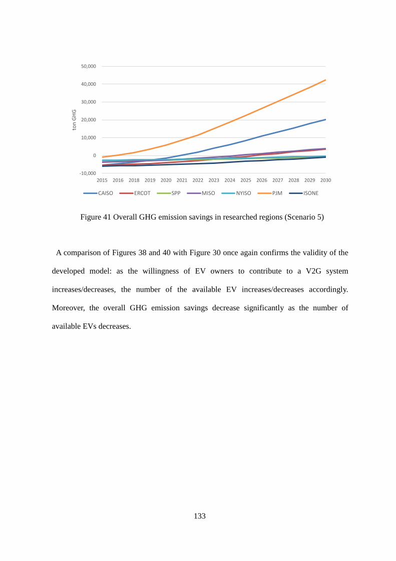
133


A comparison of Figures 38 and 40 with Figure 30 once again confirms the validity of the

developed model: as the willingness of EV owners to contribute to a V2G system

increases/decreases, the number of the available EV increases/decreases accordingly.

Moreover, the overall GHG emission savings decrease significantly as the number of

available EVs decreases.

-10,000

0

10,000

20,000

30,000

40,000

50,000

2015 2016 2018 2019 2020 2021 2022 2023 2024 2025 2026 2027 2028 2029 2030

ton

GH

G


134

6 VEHICLE-TO-GRID SYSTEMS IN THE WATER AND ENERGY

NEXUS – A SYSTEM DYNAMICS MODELLING APPROACH

A partial work of this Chapter has been submitted to the Journal of Energy

V2G is a further integration of the energy and the transportation system, utilize the battery

capacity of idled electric vehicles as grid storage, allowing them to improve the reliability of

the power grid and to accommodate larger partition of intermittent renewable power. The

research in section 4 has shown that with appropriate incentives, both

commercial/government fleets and private car owners (Noori et al., 2016) could be V2G

ancillary service carriers and gain certain amount of financial benefits. And because of the

higher efficiency of battery storage which can absorb excess energy as well as the absence of

the combustion of fossil fuel, V2G systems could significantly reduce carbon emissions

during ancillary service provision. As more and more electric vehicle options being released

to the market and charging devices being encouraged to be installed, 700 GW of wind capacity

could be integrated to the system if approximately 3% of the U.S. fleet was V2G available

(Kempton and Tomić, 2005b). And an energy system with higher renewable power

penetration will provide cleaner power source for the transportation sector and further

facilitate the shift of the electrification of the transportation system.

6.1 Introduction

Water and electricity are interconnected; the generation of electricity requires water for

cooling, and the treatment and delivery of freshwater also consumes electricity. Due to the

combustion of fossil fuels (coal, natural gas, petroleum, etc.), the electricity generation sector

is the largest single contributor to greenhouse gas (GHG) emissions in the U.S. (U.S.

Environmental Protection Agency, 2016), the second largest GHG emission contributor being

135

the transportation sector. There are currently 260 million registered vehicles in the U.S.,

approximately 11% of which are powered by alternative fuels, and the projected growth rate

of hybrid electric vehicles (HEVs) and plug-in electric vehicles (PEVs) in the U.S. are the

highest out of all other vehicle types (U.S. Energy Information Adiministration, 2017). The

electrification of transportation brings vehicles and the power grid together in a single system

and thereby reduces fossil fuel usage at the end-user phase of a vehicle, while HEVs or PEVs

can increase fuel efficiency and partially or entirely eliminate tailpipe emissions. However,

whether or not carbon emissions and/or water consumption can really be mitigated depends

on the percentage of renewable energy in the system.

The two largest renewable energy sources (wind power and solar photovoltaic (PV) power)

are both intermittent, so, more ancillary service capacity must be online to accommodate

renewable energy output and to facilitate the stability of the power grid. Vehicle-to-Grid (V2G)

systems, which serve as a further integration of the electric power and transportation sectors,

use the battery capacity of idle electric vehicles as grid storage, allowing them to improve the

reliability of the power grid and to accommodate larger partitions of intermittent renewable

power output. In addition, due to the higher efficiency of battery storage that can absorb

excess energy as well as the absence of the combustion of fossil fuels, V2G systems can

significantly reduce carbon emissions while providing ancillary services. The water

consumption rate of thermoelectric power generation varies from 100 to 700 gallon per MWh

depending on the type of cooling used (Macknick et al., 2011), and the life-cycle energy

intensity in cities is 3.3 to 3.6 MWh for every 1 million gallons of water consumed (Copeland,

2014). Since more than 80% of electricity in the U.S. is generated from coal, natural gas,

and/or nuclear power (U.S. Environmental Protection Agency, 2014a), all of which withdraw

and consume significant amounts of water for cooling purposes, V2G technology can further

136

reduce water withdrawal and water consumption rates from electricity generation. In short,

with sufficient market penetration for HEVs and PEVs, a well-developed power grid network,

and sophisticated V2G scheduling, the water-energy structure will be optimized, and overall

GHG emissions will be more effectively mitigated. V2G systems will therefore inevitably

affect and be affected by other social, economic, and environmental factors, and the various

interactions between all of these factors will change dynamically. Therefore, in this paper, a

system dynamic modelling approach is combined with a life cycle assessment (LCA) method

to study how the use of V2G systems and/or a smart grid would affect the interactions between

the passenger car transportation industry and the water-energy nexus. The system is evaluated

from the associated social, economic, and environmental perspectives, after which projections

are estimated (based on the mathematical relationships within the model), and different

policies are tested to evaluate the overall impacts and benefits of the studied V2G system. The

state of Florida has been selected as the studied region for purposes of this study, and the

simulation time of the model will run from 2000 to 2030.

6.2 Literature Review

Electricity is a unique commodity in that it has to be generated and consumed at the same

time; otherwise, any excessive electricity generation is ultimately wasted since the current

power grid lacks any means of energy storage (U.S. Energy Information Adiministration,

2000) while, if the electricity demand surges beyond the available energy generation at a

certain time point, gas combustion turbines must then be turned on or ramped up to

compensate for the added fluctuation in energy demand (Kempton and Tomić, 2005b). Studies

have shown that battery storage methods have lower response times (usually within a matter

seconds) than combustion turbine generators (Kempton and Tomić, 2005b), and the

efficiencies of such storage methods are typically one to two times higher than those of

137

traditional turbines (Lin, 2011; Makarov et al., 2012).

Renewable energy sources (wind, solar, etc.) typically emit less GHG emissions and

consume less water, but the output of renewable power in most cases is subject to significant

fluctuation. Parsons et al. (2006) studied the cost of integrating wind energy in different

Independent System Operator (ISO) and Regional Transmission Organization (RTO) regions,

and concluded that additional regulation capacity will be required as the percentage of wind

energy increases. Since the current energy system cannot sustain unlimited wind energy

generation, Bird and Lew (2012) have suggested that a wind energy penetration of

approximately 20% to 35% will be feasible given the limitations of the current power grid. A

wind intermittency study conducted by Albadi and El-Saadany (2010) reached two separate

conclusions with respect to wind energy; first, as the wind penetration grows, the cost of

ancillary service will increase significantly, and hence the economic considerations might be

a main obstacle which prevents the adoption of wind energy; and second, fast-responding

ancillary service generators can reduce the overall operational cost of wind energy generation.

Studies have been conducted to explore the feasibility of supporting wind energy integration

through V2G technology (Kempton and Tomić, 2005a, b), and another study has also

confirmed that a smart energy network with the inclusion of PEVs could help to facilitate

wind energy integration (Short and Denholm, 2006).

From the water-energy nexus’s perspective, Cooper and Sehlke (2012) have pointed out that

reducing or maintaining GHG emissions within a reasonable level will require changes in

various environmental, economic, and societal aspects, and that effective methods to reduce

water consumption include the integration of wind energy and/or solar power into the power

grid, the introduction of high-efficiency baseload coal power plants, and the development of

more efficient vehicles. In addition, a review paper (Nair et al., 2014) has reported the

138

importance of identifying the underlying complex relations between water consumption and

energy generation. A separate study carried out by Sovacool and Sovacool (2009) confirmed

the need to introduce more renewable energy into the power grid to improve the overall

efficiency of the water-energy nexus.

There is currently no available literature that either investigates or projects the environmental,

social, and economic interactions of a V2G system integrated with the future water-energy

nexus from a life cycle perspective; to address this research gap, a system dynamics model is

built in this study to simulate such a system and its relevant interactions with other

environmental, social, and economic factors, including the integration of renewable energy

technologies, as well as GHG emissions, population, health factors, and the Gross Domestic

Product (GDP). Moreover, this study will test four possible scenarios with different

assumptions representing different levels of EV adoption, V2G service participation, and

wind energy integration.

6.3 Methods

System dynamics is an approach used in today’s research to investigate complex system

problems, especially those that involve large networks with complicated dependency

relationships, feedback mechanisms, and multidimensional causal relationships. The

available literature indicates that, in order to comprehensively study a complex system such

as the U.S. transportation system or the power grid, the underlying environmental, social, and

economic consequences of any given scenario must all be taken into consideration (Lee et al.,

2012). The network of the proposed model of this study is constructed at three different scales:

First, at an individual vehicle level, the available ancillary power output and the

amount of exchanged energy both depend on the service provision time, the battery State

of Charge (SOC), and other relevant variables;

139

Second, at the electricity grid level, a V2G system not only replaces traditional gas

turbines as ancillary service providers and thereby reduces GHG emissions, but also

increases the overall ancillary service capacity within the hosting area, allowing more

intermittent wind power to be brought online;

Third, at the electricity grid and water-energy nexus level, the overall grid mix, the

average GHG emission rate, and the average water consumption rate are all interconnected

with the GDP, human health factors, and EV market penetration levels.

The outline of the overall system is shown in Figure 42 below.

Figure 42 Overall system outline

6.3.1 Scope of study, variables, and initial assumptions

The state of Florida has been selected as the researched region for purposes of this paper, as

it has the fourth largest economy in the nation with approximately 5% of the total GDP of the

U.S. (U.S. Department of Commerce, 2017b); the population of Florida is about 20 million,

making Florida the fourth most populated state in the U.S., and the majority of the electricity

140

in Florida is produced from natural gas. Although Florida is not one of the deregulated

markets where electricity transmission and generation are divided among different parties, the

state has made a significant effort to promote transportation electrification; for instance,

hybrid and electric vehicles are both exempted from high occupancy lane rules (Florida DMV,

2015), and rebates and other such incentives are also available for purchasing EVs and/or EV

charging equipment (National Conference of state Legislatures, 2015). Also, the Florida

roadway design criteria will soon include specific standards to accommodate large-scale EV

adoption rates. In addition to the aforementioned HEVs and PEVs, internal combustion engine

vehicles (ICEVs) are still going to be the main vehicle type on the market, so ICEVs are also

included in this study.

To study and reveal the underlying causal relationships of the proposed model, a causal loop

diagram is first created to illustrate the conceptual structure and qualitative relationships

within the model. As shown in Figure 43, the GDP, population, and GHG and other air

pollutant emissions all represent the macro-level economic, societal, and environmental

aspects of the system, respectively, and the water-energy nexus as it relates to the V2G system

is incorporated within this macro-level structure as well. The green loops in Figure 43

represent the major reinforcing loops, or the potentially positive effects caused by the adoption

of V2G systems; as demonstrated in these loops, the application of the V2G system allows

for the greater installation of ancillary service providers, which would therefore accommodate

more wind power; this wind power generation not only emits much less GHG/air pollutant

emissions but also requires less water for cooling purposes, and therefore less energy is

needed to deliver or to treat this reduced quantity of water; the overall reduced GHG/air

pollutant emissions then encourages policy makers to promote EV sales more effectively,

resulting in more EVs being made available for V2G services.

141

Figure 43 Causal loop diagram

Based on the developed causal loop diagram (Figure 43), the quantitative relationship among

the variables within all the loops are further divided into three sub-models:

1. The GDP, population, and passenger vehicle transportation sub-model,

2. The passenger transportation emission and V2G system sub-model, and

3. The water-energy nexus model.

Next, stock and flow diagrams are developed for each sub-model, each containing all of the

associated the variables and their mathematical relationships (Section 5.3.2 to Section 5.3.4).

Some of these variables (“exogenous variables”) are used to reference historical and/or

projected data sets that are out of the scope of this study, while the values and/or outputs of

other variables (“endogenous variables”) may change depending on logical and/or

142

mathematical relationships with other variables. The exogenous and endogenous variables

within this model are all summarized in Table 17.

This study focuses on the water consumption needed for electricity generation and on the

energy consumption required for treating and/or recovering the amount of the water lost for

cooling purposes in power plants; residential and irrigation-related water consumption are not

included because the influence of the V2G system on these activities is negligible. The authors’

previous studies have shown that V2G regulation services are economically appealing to EV

owners (Noori et al., 2016; Zhao et al., 2016a), so it is also assumed that sophisticated

infrastructure and networks will be available to aggregate all of the individual EV owners into

separate clusters with stable capacities and output rates for ancillary services provision

(Kempton and Tomić, 2005b).

143

Table 17 Endogenous variables and exogenous variables

Endogenous variables Exogenous variables

GDP,

population,

and passenger

vehicle

transportation

sub-model

GDP from the passenger car transportation

sector

GDP from the rest of the sectors

total GDP GDP increasing rate

GDP per capita reproductive lifetime

fertility rate life expectancy

maturation rates market share of passenger vehicles

death rates Percentage of HEVs, PEVs, and ICEVs

adjusted life expectancy manufacturing cost data of HEVs, PEVs,

and ICEVs

population maintenance and fuel cost data of HEVs,

PEVs, and ICEVs

number of potential drivers vehicle configuration data of HEVs, PEVs,

and ICEVs

marginal human health impact from

emissions

annual VMT

new passenger vehicle sales

number of HEVs, PEVs, and ICEVs

V2G promotion effect percentage

Passenger

transportation

emission and

V2G system

sub-model

annual PEV GHG emissions average GHG emission rate before 2015

annual HEV GHG emissions average traditional air emission rate before

2015

annual ICEV GHG emissions

annual PEV traditional air emissions battery manufacturing GHG emission rate

annual HEV traditional air emissions battery manufacturing traditional air

emission rate

annual ICEV traditional air emissions gasoline upstream and tailpipe GHG

emission rate

electricity mix GHG emissions gasoline upstream and tailpipe traditional

air emission rate

electricity mix traditional air emissions V2G ancillary service related data

V2G emission savings

Water-energy

nexus sub-

model

HEV and PEV ancillary service capacity HEV and PEV available power

renewable power capacity growth ancillary service requirement ratio

capacity of different power sources emission rate of different electricity sources

annual generation of different power sources water withdrawal rate of electricity sources

future electricity GHG emission rate water evaporation rate

future electricity traditional air emission rate energy intensity ratio of water treatment

saline water withdrawal

fresh water withdrawal

fresh water evaporation

electricity consumption for water treatment

144

6.3.2 GDP, population, and passenger vehicle transportation sub-model

Each of the individual sub-models are depicted separately; grey variables indicate variables

that are also connected to one or more other variables within the model, and red, green, and

light blue variables indicate the main inflows or outflows to other sub-models, as discussed

in further detail with respect to each of the relevant figures. In this section, the GDP is

separated into the contribution of the passenger car transportation industry to the GDP and the

combined contribution of all other economic sectors to the GDP. As shown in Figure 44, the

“total GDP” variable receives inputs from both the “GDP of passenger car transportation”

variable and the “GDP from the rest of the sectors” variable. Data for the overall GDP of the

state of Florida is available from the literature (Federal Reserve Bank of St. Louis, 2016). The

GDP data of other sectors prior to 2015 is likewise obtained from the Bureau of Economic

and Business Reserve (2015), and used in the model as a lookup function since this portion

of the GDP is beyond the scope of this study. GDP growth is represented in terms of annual

GDP growth as a stock that increases relative to a certain rate each year. It is assumed that

there will be a 2.9% GDP increasing rate after 2015 (U.S. Department of Commerce, 2017a).

The annual GDP of the passenger car transportation sector consists of the manufacturing cost

of all of the cars that are sold in a given year and their associated yearly operation costs; the

relevant variables are shown as grey variables in Figure 44 and are illustrated in further detail

in Figure 46, while the relevant detailed data and data sources are listed in Table 2.

145

Figure 44 GDP stock-flow diagram

In Figure 44, the red variable indicates that the GDP of passenger car manufacturing is

calculated based on the new car sales in each year. On the other hand, the outgoing “GDP per

capita” variable (the green variable in Figure 44) is calculated by dividing the total GDP by

the overall population, which is shown in Figure 45. The “GDP per capita” variable affects

two critical variables (the fertility rate and new passenger vehicle sales), which are both

illustrated further in Figure 45. The fertility rate is a deterministic factor for the population

section of the model, and its mathematical formula is as shown in Equation 24 below.

𝑓𝑒𝑟𝑡𝑖𝑙𝑖𝑡𝑦 𝑟𝑎𝑡𝑒 = (𝐺𝐷𝑃 𝑝𝑒𝑟 𝑐𝑎𝑝𝑖𝑡𝑎 × 9.57) − (0.233 × 𝑎𝑑𝑗𝑢𝑠𝑡𝑒𝑑 𝑙𝑖𝑓𝑒 𝑒𝑥𝑝𝑒𝑐𝑡𝑎𝑛𝑐𝑦) + 19.97 ( 2 4 )

The adjusted life expectancy is a function of the projected life expectancy (State of Florida

Department of Health, 2012), which is in turn affected by the marginal human health impact

associated with the passenger car transportation sector, the variable for which is shown in

146

light blue in Figure 45. The verification of Equation 24 is discussed in detail in Section 6.4.

The population section is a multi-stage stock and flow diagram that simulates individuals

being born and progressing through each life stage. The births of the population is a function

of “population 15 to 44”, the fertility rate, and the reproductive lifetime (which is assumed to

be 30). The two important outputs of the population section is the overall population, which

is connected to the “GDP per capita” variable as part of a feedback loop, and the number of

potential drivers, which is assumed to be equal to the total portion of the population that is

older than the age of 15. Based on historical data for passenger vehicle market shares (Bureau

of Transportation Statistics, 2015b) and the output from the “GDP per capita” and the “number

of potential drivers”, the “new passenger vehicle sales” variable is calculated as shown in

Equation 25 below:

𝑛𝑒𝑤 𝑝𝑎𝑠𝑠𝑒𝑛𝑔𝑒𝑟 𝑣𝑒ℎ𝑖𝑐𝑙𝑒 𝑠𝑎𝑙𝑒𝑠

= (𝑚𝑎𝑟𝑘𝑒𝑡 𝑠ℎ𝑎𝑟𝑒 𝑜𝑓 𝑝𝑎𝑠𝑠𝑒𝑛𝑔𝑒𝑟 𝑣𝑒ℎ𝑖𝑐𝑙𝑒 (𝑇𝑖𝑚𝑒) ×

(𝐺𝐷𝑃 𝑝𝑒𝑟 𝑐𝑎𝑝𝑖𝑡𝑎×7.3284×107)−(1.2596×𝑛𝑢𝑚𝑏𝑒𝑟 𝑜𝑓 𝑝𝑜𝑡𝑒𝑛𝑡𝑖𝑎𝑙 𝑑𝑟𝑖𝑣𝑒𝑟𝑠)+(3.3242×107)

5) − 3 × 105 ( 2 5 )

Like with Equation 24, the verification of Equation 25 is also explained in more detail in

Section 6.4. The overall numbers of HEVs, PEVs, and ICEVs are each based on the

percentages of the overall sales rate pertaining to each vehicle type, which are adjusted as

necessary in different scenarios as discussed further in Section 6.3.5. In addition, a

sophisticated EV infrastructure with economic benefits and emission mitigations from V2G

services may further increase the market share of EVs, so the market shares of HEVs and

PEVs are both also marginally affected by the variable “V2G promotion effect percentage”.

147

Figure 45 Population and vehicle market stock-flow diagram

Figure 46 Passenger car related cost stock-flow diagram

6.3.3 Passenger transportation emission and V2G system sub-model

The life cycle GHG emissions and traditional air pollutant emissions of the passenger car

transportation sector and of the V2G system are analyzed and modeled in this section. To

simplify the necessary calculations, GHG and air pollutant emissions are each measured in

terms of CO2 and Particular Matter (PM) emissions, respectively. The vehicle configuration

and all parameters related to emissions and costs are all summarized in Table 18.

148

Table 18 Data sources for critical parameters

Parameter Value and unit Data source

ICEV price $28,465 to $21484 (2000 to 2030) (U.S. Department of

Energy, 2013a)

HEV price $35,581 to $26,855 (2000 to 2030) (Papaioannou, 2015)

PEV price $50,000 to $35,000 (2000 to 2030) (UCLA Luskin Center,

2012)

manufacturing cost/retail price

ratio

0.8 (Samaras and

Meisterling, 2008)

annual VMT 9,516 to 12,866 miles (2000 to 2030) (Florida Department of


average lifetime mileage 200,000 miles (Florida Department of


ICEV and HEV maintenance

and tire cost

0.053 to 0.0703 $/mile (2000 to 2030) (Bureau of

Transportation

Statistics, 2015c)

PEV maintenance and tire cost 70% of ICV and HEV maintenance cost (Gallo and Tomic,

2013)

average ICEV MPG 28.5 to 39.6 mile per gallon (2000 to

2030)

(Bureau of

Transportation

Statistics, 2015a)

average HEV MPG 40 to 70 mile per gallon (2000 to 2030) (U.S. Energy

Information

Adiministration, 2015f)

average PEV fuel efficiency 0.35 kWh/mile (U.S. Department of

Energy, 2013b)

PEV battery capacity 30 kWh (Nissan, 2015)

battery unit price 600 to 300 $/kWh (Gallo and Tomic,

2013)

gasoline price (historical and

projected)

1.513 to 2.92 $/gallon (U.S. Energy

Information


electricity price (historical and

projected)

0.0757 to 0.1153 $/kWh (U.S. Energy

Information

Adiministration, 2015c)

battery manufacturing GHG

emission rate

0.14 ton CO2/kWh (Kim et al., 2016)

battery manufacturing PM

emission rate

0.01 ton PM/kWh (Carnegie Mellon

University Green

Design Initiative, 2003)

PEV buffering range 30 miles (Kurani et al., 1994)

V2G dispatch time 0.3 hours (Kempton and Tomić,

2005a; Zhao et al.,

2016a, 2017)

DC to AC conversion

efficiency

0.93 (Kempton and Tomić,

2005a)

Dispatch time 0.3 (Kempton and Tomić,

2005a)

149

Figure 47 illustrates the calculations required for life cycle GHG emissions and traditional

air pollutant (i.e. PM) emissions. The concept of the LCA is to consider all relevant upstream

and downstream environmental impacts. For HEVs and ICEVs, the overall emissions consist

of those due to gasoline production and tailpipe emissions, and for PEVs, the overall

emissions include those associated with electricity generation and battery manufacturing. For

example, Equations 26 and 27 are used to calculate the annual PEV GHG emissions and the

annual ICEV GHG emissions, respectively:

𝑎𝑛𝑛𝑢𝑎𝑙 𝑃𝐸𝑉 𝐺𝐻𝐺 𝑒𝑚𝑖𝑠𝑠𝑖𝑜𝑛𝑠 = (𝑎𝑛𝑛𝑢𝑎𝑙 𝑉𝑀𝑇(𝑇𝑖𝑚𝑒) ×𝑎𝑣𝑒𝑟𝑎𝑔𝑒 𝑃𝐸𝑉 𝑓𝑢𝑒𝑙 𝑒𝑐𝑜𝑛𝑜𝑚𝑦 × 𝑒𝑙𝑒𝑐𝑡𝑟𝑖𝑐𝑖𝑡𝑦 𝑚𝑖𝑥 𝐺𝐻𝐺 𝑒𝑚𝑖𝑠𝑠𝑖𝑜𝑛 𝑟𝑎𝑡𝑒) +

(𝑏𝑎𝑡𝑡𝑒𝑟𝑦 𝑚𝑎𝑛𝑢𝑓𝑎𝑐𝑡𝑢𝑟𝑖𝑛𝑔 𝐺𝐻𝐺 𝑒𝑚𝑖𝑠𝑠𝑖𝑜𝑛 𝑟𝑎𝑡𝑒 × 𝑃𝐸𝑉 𝑏𝑎𝑡𝑡𝑒𝑟𝑦 𝑐𝑎𝑝𝑎𝑐𝑖𝑡𝑦) ( 2 6 )

𝑎𝑛𝑛𝑢𝑎𝑙 𝐼𝐶𝑉 𝐺𝐻𝐺 𝑒𝑚𝑖𝑠𝑠𝑖𝑜𝑛 = 𝑎𝑛𝑛𝑢𝑎𝑙 𝑉𝑀𝑇(𝑇𝑖𝑚𝑒) × 𝑎𝑣𝑒𝑟𝑎𝑔𝑒 𝐼𝐶𝑉 𝑀𝑃𝐺(𝑇𝑖𝑚𝑒) ×(𝑔𝑎𝑠𝑜𝑙𝑖𝑛𝑒 𝑠𝑢𝑝𝑝𝑙𝑦 𝐺𝐻𝐺 𝑒𝑚𝑖𝑠𝑠𝑖𝑜𝑛 𝑟𝑎𝑡𝑒 + 𝑔𝑎𝑠𝑜𝑙𝑖𝑛𝑒 𝑡𝑎𝑖𝑙𝑝𝑖𝑝𝑒 𝐺𝐻𝐺 𝑒𝑚𝑖𝑠𝑠𝑖𝑜𝑛 𝑟𝑎𝑡𝑒) ( 2 7 )

It should be noted that the GHG emission rate of the electricity mix as described in Equation

26 is a dynamic function related to the market shares of each energy source available to the

power grid and their corresponding emission rates. This overall emission rate for the Florida

power grid is knows from 2000 to 2016, and starting from 2017, the evaluated emission rate

fully reflects the impacts of the rest of the model on the overall power grid emission rate.

150

Figure 47 Stock-flow diagram for the life cycle GHG emissions and traditional air

emissions of HEVs, PEVs, and ICEVs

Figure 48 simulates the emission savings of the V2G system with respect to the power grid,

as well as the potential availability of ancillary service capacity from PEVs and HEVs. Based

on the literature (Kempton and Tomić, 2005a, b) and the authors’ previous studies (Zhao et

al., 2016a, 2017; Zhao and Tatari, 2015), individual EVs are aggregated in V2G systems and

serve as additional storage capacity, so when the grid operator needs a certain amount of

energy to balance off a sudden and unpredicted demand peak, the electricity previously stored

in the EVs’ batteries is extracted and supplied back to the power grid; likewise, whenever the

energy demand is lower than the standard energy supply rate, the extra electricity can be stored

in the vehicles’ batteries for the next cycle or until it is needed again. This process is also

called regulation services, and providing such regulation services using a V2G system can

effectively reduce the need to use traditional combustion turbines (gas or oil powered), which

have fast responding times but generate two to three times as much GHG emissions. The

electricity exchanged through a vehicle’s battery for V2G regulation services is determined

151

by its available power and the V2G provision time, as shown in Equation 28:

𝑃𝐸𝑉𝑎𝑝 =(𝐵𝑐𝑎𝑝𝑎𝑐𝑖𝑡𝑦 −

𝐷𝑎𝑖𝑙𝑦𝑣𝑚𝑡 −𝑅𝑎𝑛𝑔𝑒𝑏𝑢𝑓𝑓𝑒𝑟

𝐹𝑒 ) 𝐶𝑒

𝑇𝑑𝑖𝑠𝑝𝑎𝑡𝑐ℎ ( 2 8 )

Where PEVap is the “PEV available power” variable, Bcapacity is the PEV battery capacity,

Dailyvmt is the annual VMT divided by 365, Rangebuffer is the buffering range, Fe is the average

fuel efficiency of PEVs, Ce is the conversion efficiency (which is used to represent the energy

loss during the process), and Tdispatch is the average time interval of each regulation cycle. The

values and data sources of these parameters have all already been listed in Table 18. Based on

the internal calculations for this section of the model and the authors’ previous study (Zhao et

al., 2017), the available power of PEVs for regulation services is approximately 30 kW. On

the other hand, the available power of HEVs is difficult to simulate because, during daily

driving routines, HEV engines can consume the onboard gasoline to recharge the battery once

the electric range is reached, so it is assumed that the HEVs in this model have a fixed

available power of 15 kWh.

The V2G emission savings from each participating HEV or PEV per night is calculated by

multiplying the available power in each vehicle by the V2G service provision time. Existing

data indicates that an EV providing regulation services may receive and respond to 30 to 40

regulation requests (including regulation up and regulation down requests), and each cycle

lasts approximately 3.6 to 9 minutes (Kempton et al., 2008), meaning that the overall service

provision time is assumed to be 3.675 hours per night. The overall emission savings can be

calculated by multiplying the emission savings per vehicle by the number of EVs and by the

participation ratio of these EVs. The owner participation ratio is discussed in further detail

with respect to the scenarios discussed in Section 6.3.5.

In addition, the “marginal human health impact from passenger vehicle transportation”

152

variable (the light blue variable in both Figure 47 and Figure 48) indicates that the life cycle

emissions of all of the considered research cars and the V2G emission savings will both

contribute to the overall emission rates of the entire modeled system. The outgoing variable

“renewable capacity growth” (shown in purple in Figure 48 and Figure 49) indicates that the

overall available ancillary service capacity/power can be used to encourage renewable power

integration, and this relationship is further discussed in the water-energy nexus sub-model

(Section 6.3.4). Moreover, a restriction variable (“max wind power capacity”) is included to

ensure that the wind power capacity does not exceed a certain ratio; this ratio is regulated

based the scenarios discussed in Section 6.3.5.

Figure 48 Stock-flow diagram for GHG emission savings and traditional air emission

savings from the use of V2G regulation services

6.3.4 Water-energy nexus

The structure of the water-energy nexus with ancillary service support from V2G regulation

service is illustrated in Figure 49 and Figure 50. Although there is very little wind power

153

currently online, this model explores the system’s reaction to the introduction of V2G systems

as V2G regulation service carriers, which will each allow the current grid to accommodate

more wind power without significantly increasing the cost of energy generation.

To accommodate a large amount of wind power, the required ancillary service capacity will

be approximately 6% of the newly integrated power capacity (Hudson et al., 2001; Kempton

and Tomić, 2005b). One of the main assumptions of this study is that, instead of deploying

combustion gas turbines, the required ancillary services are all provided using all of the

participated HEVs and PEVs, and with respect to the “renewable capacity growth” variable

(shown in purple in Figure 49), an “if then else” function is used in this variable to simulate

the wind power that can be supported by V2G regulation service from 2000 to 2030:

𝑅𝑒𝑛𝑒𝑤𝑎𝑏𝑙𝑒 𝑐𝑎𝑝𝑎𝑐𝑖𝑡𝑦 𝑔𝑟𝑜𝑤𝑡ℎ = 𝐼𝐹 𝑇𝐻𝐸𝑁 𝐸𝐿𝑆𝐸

(𝑇𝑖𝑚𝑒 < 2016 , 0,𝐻𝐸𝑉 𝑎𝑛𝑐𝑖𝑙𝑙𝑎𝑟𝑦 𝑠𝑒𝑟𝑣𝑖𝑐𝑒 𝑐𝑎𝑝𝑎𝑐𝑖𝑡𝑦+𝑃𝐸𝑉 𝑎𝑛𝑐𝑖𝑙𝑙𝑎𝑟𝑦 𝑠𝑒𝑟𝑣𝑖𝑐𝑒 𝑐𝑎𝑝𝑎𝑐𝑖𝑡𝑦

𝑎𝑛𝑐𝑖𝑙𝑙𝑎𝑟𝑦 𝑠𝑒𝑟𝑣𝑖𝑐𝑒 𝑟𝑒𝑞𝑢𝑖𝑟𝑒𝑚𝑒𝑛𝑡 𝑟𝑎𝑡𝑖𝑜) ( 2 9 )

Where the value of the “ancillary service requirement ratio” variable is 6%. Since the market

penetration of EVs with grid accessibility increased significantly approximately between the

year 2015 and the year 2016 (Alternative Fuel Data Center, 2015), it is assumed that the use

of V2G services is available after 2015 and that, with the additional ancillary service capacity,

the associated increase in wind power market penetration is evenly distributed over the

following 15 years (from 2016 to 2030). In addition, this gradual increase in wind power

effectively replaces the original thermoelectric power capacity, and it is assumed that this

replacement ratio is based on the original ratio of each electric power source. The five stock

and flow components in this section each indicate, with respect to each energy source, the

causal flow from the rate of increase in power capacity to the total power capacity in kW

before finally leading to the total energy generation in kWh. However, the future relationship

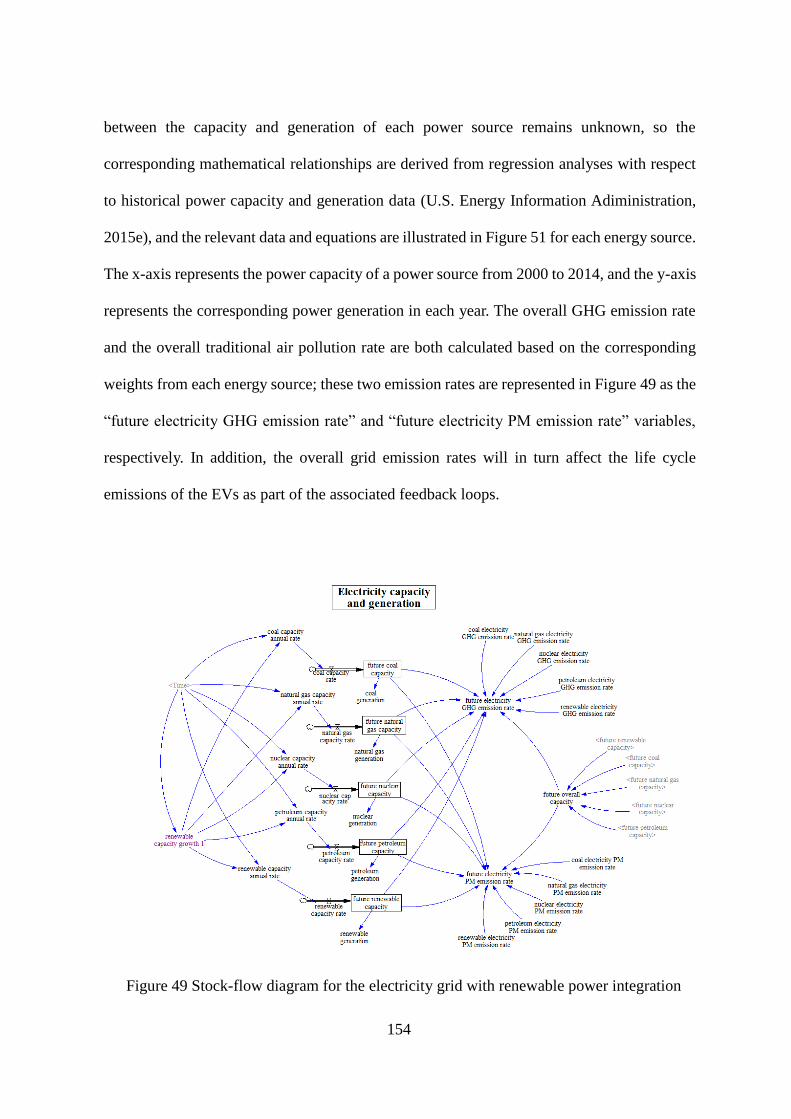
154

between the capacity and generation of each power source remains unknown, so the

corresponding mathematical relationships are derived from regression analyses with respect

to historical power capacity and generation data (U.S. Energy Information Adiministration,

2015e), and the relevant data and equations are illustrated in Figure 51 for each energy source.

The x-axis represents the power capacity of a power source from 2000 to 2014, and the y-axis

represents the corresponding power generation in each year. The overall GHG emission rate

and the overall traditional air pollution rate are both calculated based on the corresponding

weights from each energy source; these two emission rates are represented in Figure 49 as the

“future electricity GHG emission rate” and “future electricity PM emission rate” variables,

respectively. In addition, the overall grid emission rates will in turn affect the life cycle

emissions of the EVs as part of the associated feedback loops.

Figure 49 Stock-flow diagram for the electricity grid with renewable power integration

155

The water consumption rates for power plant cooling are modeled in Figure 50. In Florida,

surface water is the primary source of the water used for electricity generation (Borisova and

Rogers, 2014), and 7% of all water consumed for cooling purposes is fresh water while 93%

is saline water (Scroggs, 2014). Therefore, the water consumption rates of each energy source

are derived from the literature (Macknick et al., 2011; Torcellini et al., 2003), multiplied by

the total generation from each corresponding energy source, and distributed among the two

stock and flow sections in Figure 50 to reflect the respective consumption rates for saline

water and for freshwater. The freshwater is lost through evaporation, and the amount of energy

required for the treatment of the consumed fresh water is obtained using the evaporation rate

and the energy intensity ratio (Copeland, 2014).

The energy consumption and air emission rates due to water consumption and treatment are

calculated in this section, along with the emissions from the passenger car sector due to the

combustion of gasoline (Figure 47), the emission savings from providing V2G services using

PEVs (Figure 48), and the emissions from the power grid and from the charging of the newly

adopted PEVs (Figure 47 and Figure 49, respectively), after which all of the calculated

emission rates and emission savings are connected back to the variable “marginal human

health impact from passenger vehicle transportation”. Lastly, based on the estimated human

health impact factors of GHG emissions and traditional air emissions (Onat et al., 2016a), all

of the aforementioned emissions are translated into human health impacts simulated as

reductions in life expectancy (Figure 52).

156

Figure 50 Stock-flow diagram for water consumption for thermoelectric generation

157

Figure 51 Electricity capacity and generation regression graphs (x-axis = capacity in MW; y-axis = generation in MWh)

y = 2072.4x + 1E+08

0

50,000,000

100,000,000

150,000,000

200,000,000

250,000,000

30,000 35,000 40,000 45,000 50,000 55,000

Coal power capacity and generationy = 4500.3x - 8E+06

0

20,000,000

40,000,000

60,000,000

80,000,000

100,000,000

120,000,000

140,000,000

160,000,000

0 5,000 10,000 15,000 20,000 25,000 30,000 35,000

Natural gas power capacity and generation

y = -184373x + 8E+08

0

5,000,000

10,000,000

15,000,000

20,000,000

25,000,000

30,000,000

35,000,000

40,000,000

3,895 3,900 3,905 3,910 3,915 3,920 3,925 3,930

Nuclear power capacity and generationy = 42140e0.0005x

0

5,000,000

10,000,000

15,000,000

20,000,000

25,000,000

30,000,000

35,000,000

40,000,000

45,000,000

0 2,000 4,000 6,000 8,000 10,000 12,000 14,000

Petroleum power capacity and generation

158

Figure 52 Summary of all the variables with emission impacts

6.3.5 Scenarios

In this model, the future market penetration rates of HEVs and PEVs, the V2G regulation

service participation ratio, and the maximum wind power percentage are all included as

exogenous variables and these variables are critical indicators of the overall sustainability

level of the transportation-water-energy nexus. As indicated by the feedback loops in this

model, these indicators are all positively related; for instance, a larger EV user base would

provide more potential customers and/or market scale for the use of V2G technology; with

the increased adoption of V2G regulation services, the storage capacity and response times of

the power grid would both be improved; furthermore, with more clean energy (e.g. wind

energy) being integrated into the power grid, the overall air pollutant emission rate of

electricity generation can be reduced, further reducing the life cycle emissions of EVs. Hence,

the following assumptions are made in order to test the reaction of the model to different

realistic scenarios and/or policies:

First, based on historical data with respect to HEV and PEV sales (Block et al., 2015), the

159

baseline HEV and PEV percentages are assumed to have an increasing trend in future years,

as illustrated in Figure 53.

Figure 53 Historical and projected HEV and PEV market penetration rates

The solid line in Figure 53 indicates the historical data, while the dashed line indicates the

projected future trend. The assumed increasing rate in the baseline scenario (i.e. the most

likely scenario) is 0.2% for HEV and 0.19% for PEV, based on their respective average

increasing rates from 2010 to 2014. In addition, three more increasing rates are tested to reflect

three other possible scenarios, one scenario being more conservative than the baseline

scenario while the other two scenarios assume higher market penetration rates for both EV

types; the projected increasing rates for both EV types are set at 0.1% for the more

conservative scenario and at 0.3% and 0.4% for the two more optimistic scenarios.

The willingness ratio for V2G regulation service participation has been discussed in the

literature, but can vary significantly. Hidrue and Parsons (2015) have argued that 17.8% of

EV owners would be willing to participate, although this number can also be as high as 52.8 %

(Parsons et al., 2014), while a more conservative participation ratio of 3% to 4% has been

0

1

2

3

4

5

6

7

20

07

20

08

20

09

20

10

20

11

20

12

20

13

20

14

20

15

20

16

20

17

20

18

20

19

20

20

20

21

20

22

20

23

20

24

20

25

20

26

20

27

20

28

20

29

20

30

Per

cen

t

HEV and PEV projection

HEV PEV

160

used in a previous study (Zhao et al., 2017). In this study, the baseline EV owner participation

ratio is conservatively assumed to be 1%; this value is set as 0.5% for the low-projection

scenario and at 2% and 4% for the two more optimistic scenarios.

The National Renewable Energy Laboratory predicts a market share of 20% for wind energy

by 2030 (Lindenberg et al., 2008), so based on this projection, the maximum wind energy

market penetration levels will be set to 15% for the low-projection scenario, 20% for the

baseline scenario, and 25% and 30% for the two high-projection scenarios.

The selected parameters for each of the four scenarios are summarized in Table 19 for three

separate. It should be noted that the values specified in Table 19 apply to both HEVs and

PEVs.

Table 19 Assumptions of the scenarios

HEV and PEV

increasing rate

HEV and PEV

V2G participation

ratio

Maximum

wind ratio

conservative scenario 0.1 0.005 0.15

baseline scenario 0.19 for HEVs

0.20 for PEVs

0.01 0.20

high projection scenario 0.3 0.02 0.30

maximum projection scenario 0.4 0.04 0.40

6.4 Model validation and verification

The model is verified and validated from three different angles:

First, the critical inter-section equations that deliver the environmental and/or economic

impacts to variables such as population in the social section of the model are verified

by plugging in real-world data.

Second, the outputs (i.e. calculation results) of the applicable variables are compared

with real world historical data and/or projections.

Third, since the V2G system (which mainly impacts renewable energy capacity) has

161

not yet been adopted in the real world, the ranges of environmentally oriented results

of the model are compared with the corresponding real world projections.

The first two angles are discussed in this section, and the range check for the third angle is

discussed in more detail in the “Results and discussion” section (Section 6.5).

In the GDP, population, and vehicle market section of the model (Figures 44 and 45),

Equation 24 links the GDP-related variables to the population section through the relationship

between the GDP per capita and the fertility rate of the population. Likewise, Equation 25

links both the GDP section and the population section, and also determines the amount of

passenger vehicle sales (which is a critical element of the model), so to verify the model,

Equations 24 and 25 are first tested by applying both equations with existing data from 2000

to 2015. The historical GDP data for Florida is obtained from the Federal Reserve Bank of St.

Louis (2016), while the historical population data is obtained from the World Population

Review (2015), the life expectancy data is provided by the (Florida Department of Health,

2015), and the real-world fertility rate data for the state of Florida is also likewise derived

from the literature (National Center for Health Statistics, 2017). The existing data sets for

GDP per capita and for life expectancy are both plugged into Equation 24 and are then

compared with the real-world fertility data through a regression analysis. The results of this

analysis indicate that the results of the above-cited calculations are coherent with respect to

the corresponding real-world data (R2 = 0.67). This comparison is also shown visually in

Figure 54.

162

Figure 54 Fertility rate comparison between real-world data and model calculations

Likewise, for Equation 25, the number of potential drivers (Florida population aged 16 or

older), GDP per capita, and overall population data are all derived from the literature as

previously cited, and are then applied to Equation 25 and then compared to the actual annual

vehicle sales from 2000 to 2015 (Federal Reserve Bank of St. Louis, 2017). This comparison

(regression result R2=0.52) is shown visually in Figure 55.

2000 2001 2002 2003 2004 2005 2006 2007 2008 2009 2010 2011 2012 2013 2014 2015

Real-world data 2.11 2.10 2.06 2.06 1.96 2.15 2.06 1.97 1.91 1.79 1.88 1.83 1.84 1.83 1.84 1.84

Model calculation 2.15 2.16 1.99 2 2.02 2.06 2.08 2.11 2.05 1.92 1.83 1.8 1.77 1.77 1.77 1.77

0.00

0.50

1.00

1.50

2.00

2.50

Fertility rate: model calcualtion and real-world data

Real-world data Model calculation

163

Figure 55 Annual vehicle sales comparison between real-world data and model

calculations

In addition to the verification of the two critical equations, ANOVA tests are applied to the

model outputs and actual historical/projected data for GDP and population.

The total GDP as simulated in this model consists of the GDP contribution from the

passenger car sector and the overall GDP contribution from all other economic sectors, so in

order to verify the structure and the mathematical relationships among these variables, the

historical GDP of Florida (Federal Reserve Bank of St. Louis, 2016) and the projected GDP

growth rate (U.S. Department of Commerce, 2017a) are both analyzed along with the GDP

output (in millions of dollars) from the model. The ANOVA test results are summarized in

Table 20, and the results in this table show that the F value is much less than the F critical

value, meaning that there is no significant statistical difference between the real-world data

and the model output.

2000

2001

2002

2003

2004

2005

2006

2007

2008

2009

2010

2011

2012

2013

2014

2015

Model calculation 1.20 1.22 1.25 1.21 1.23 1.31 1.33 1.29 1.14 1.00 1.00 0.98 1.00 1.03 1.07 1.14

Real-world data 1.30 1.28 1.25 1.24 1.26 1.27 1.25 1.20 0.99 0.77 0.86 0.96 1.08 1.16 1.23 1.30

0.60

0.70

0.80

0.90

1.00

1.10

1.20

1.30

1.40M

illio

n

Annual vehicle sales: model calculation and real-world data

Model calculation Real-world data

164

Table 20 ANOVA test of GDP data sets

Groups Count Sum Average Variance

Real-

world

GDP 31 27998326 903171.7979 60758568314 Baseline

output

GDP 31 28808405 929303.3871 66405803858

ANOVA Source of

Variation SS df MS F P-value F crit

Between

Groups 10584329256 1 10584329256 0.166466898 0.684723 4.001191

Within

Groups 3.81493E+12 60 63582186086

Total 3.82552E+12 61

The population is modeled through a series of stocks and flows (Figure 45), so to verify this

section, the historical and projected populations of the State of Florida (World Population

Review, 2015) are compared with the corresponding output from the variable “population” in

the model. The results of the ANOVA test for this comparison are shown in Table 21; this

table shows that the F value for this comparison is significantly less than the critical F value,

indicating that there is no significant statistical difference between the model output for the

population and the actual Florida population data.

165

Table 21 ANOVA test of population data sets


Real-world

population 31 638898995 20609644.99

9.28314E+1

2 Baseline

output

population 31 659131300 21262300

5.14038E+1

2

ANOVA Source of


Between

Groups

6.60236E+1

2 1

6.60236E+1

2 0.915498604

0.34249

9

4.00119

1

Within

Groups

4.32706E+1

4 60

7.21176E+1

2

Total

4.39308E+1

4 61

6.5 Results and discussion

First, the model results for the GDP, population, and overall GHG emissions are shown in

Figure 56, Figure 57 and Figure 58, respectively; these variables serve as the primary

indicators of the economic, social, and environmental aspects of the modeled system. It can

be concluded from Figure 56 that, in the baseline (most likely) scenario, the overall GDP of

Florida increases from $500 billion to $1,400 billion, but it is also evident that the overall

GDP is not affected significantly by increasing/decreasing either the EV market penetration

or the V2G participation ratio. The columns on the right side represent the changes in the

overall GDP in each of the other three scenarios. The conservative assumptions lead to a slight

decrease in GDP; meanwhile, in more optimistic scenarios with respect to EV market

penetration, the V2G participation ratio, and the maximum wind energy market share, the

overall GDP grows accordingly. However, at a trillion-level scale, variations at a hundred-

million-level scale are barely visible on the charts. Also, as previously noted, the GDP as

simulated in this model is divided into that of the passenger car sector and that of all other

sectors combined, the latter of which is simulated as an exogenous lookup function and

therefore does not change under any scenario assumptions, so the variations in GDP indicated

166

in Figure 56 are due entirely to the increased market penetration levels of HEVs and PEVs,

although the market shares of HEVs and PEVs are both still under 10% (Figure 44 and Figure

45), so it can be concluded that, although EVs are considered to have lower maintenance cost,

a relatively small percentage of EV still results in a positive impact on the economy.

Figure 57 shows model results with respect to the population. In the baseline scenario, from

2000 to 2030, the population of Florida gradually increases from 17.3 million to 24.8 million.

As with the GDP results (Figure 56), the impacts from the GDP and the overall emission rates

are almost negligible, with a reduction of approximately 100 relative to a 20-million level

base population). By studying the connections and mathematical relationships between the

applicable variables, two reasons can be found for this result:

First, as a deterministic factor for population, the fertility rate is calculated based on

the variables “GDP per capita” and “adjusted life expectancy”, but since the GDP is only

slightly affected by other variables, the model output for GDP per capita (Figure 58) is

not affected by changing any scenario assumptions.

Second, the variable “marginal human health impact from passenger vehicle

transportation” (first introduced in Figure 45) does reflect changes at a certain scale

(Figure 58) and is a dimensionless factor in the model, but when connected to the

“adjusted life expectancy” variable, the value of the variable is divided by the total

population, meaning that very little of this change translates as a change in the adjusted

life expectancy.

167

Figure 56 GDP results of four scenarios

Figure 57 Population results of four scenarios

-300

-200

-100

0

100

200

300

400

500

600

0

200,000

400,000

600,000

800,000

1,000,000

1,200,000

1,400,000

1,600,000

20

002

001

20

022

003

20

042

005

20

062

007

20

082

009

20

102

011

20

122

013

20

142

015

20

162

017

20

182

019

20

202

021

20

222

023

20

242

025

20

262

027

20

282

029

20

30

mill

ion

$

mill

ion

$Baseline GDP and scenario variations

high projection scenario variation maximum projection scenario variation

conservative variation baseline scenario

-250

-200

-150

-100

-50

0

50

100

150

0

5,000,000

10,000,000

15,000,000

20,000,000

25,000,000

30,000,000

20

00

20

01

20

02

20

03

20

04

20

05

20

06

20

07

20

08

20

09

20

10

20

11

20

12

20

13

20

14

20

15

20

16

20

17

20

18

20

19

20

20

20

21

20

22

20

23

20

24

20

25

20

26

20

27

20

28

20

29

20

30

Baseline population and scenario variations

high projection scenario variation maximum projection scenario variation

conservative variation baseline scenario

168

Figure 58 Results for GDP per capita and the marginal human impact factor

Unlike the results for the GDP and for the population, the overall GHG emission rate from

the entire passenger car section and from water-energy nexus is sensitive to the different

scenario assumptions previously discussed. The overall GHG emission rate is modeled as the

total sum of the life-cycle GHG emissions of all vehicles (including HEVs, PEVs, and ICEVs),

the GHG emissions due to electricity generation, and the GHG emissions resulting from the

necessary energy consumption for water treatment. As shown in Figure 59, with the adoption

of V2G systems in 2015, the increasing trend in overall GHG emissions is visibly slowed

down. According to the result prior to 2015, which were calculated using historical data, the

overall GHG emission rate from both passenger transportation and electricity generation

increased from 202 million tons to 254 million tons, and there is a high possibility that this

number will continue to increase without further policy intervention, as there has currently

been no significant change in energy infrastructure and no significant market shares of clean

power sources for the passenger transportation sector have yet been introduced. Based on

conservative market estimates (conservative scenario in Table 19), the 0.1% HEV and PEV

increasing trend leads to 2030 market penetration levels of 4.3% for HEVs and 2.3% for PEVs.

If 0.5% of these EV owners are willing to participate in V2G regulation services, the overall

GHG emissions can be stabilized at a level of 260 million tons without requiring a significant

169

increase; it must also be noted that this scenario is most likely to be achieved in the future if

large-scale off-shore wind power capacity achieves a market share of up to 15% of the overall

power grid capacity.

The results of the conservative and baseline scenarios are identical, but in scenarios with

more optimistic projections for EV and wind power market penetration, GHG emissions after

the year 2023 decrease to less than the current GHG emission rate of 260 million tons. In the

maximum EV adoption/wind power integration scenario, where the final (2030) market

penetration levels are at their highest estimated values, the corresponding 2030 market shares

are 9.15% for HEVs, 7.12% for PEVs, and 40% for wind power capacity, while the V2G

participation ratio is estimated at 4%; under these conditions, approximately 10 million tons

of GHG emissions can be saved.

In addition, it is noted that the total GHG emission rate of the entire transportation sector

(not just the passenger car sector) and the electricity generation sector is about 268 million

ton in 2007 (Florida Department of Environmental Protection, 2010), confirming that the

results of the model fall within a reasonable range.

170

Figure 59 Overall GHG emission results of four scenarios

Significant amount of GHG emissions can be mitigated in the maximum projection scenario

because of the reinforcing loop activated through the use a V2G system. In this feedback loop,

the growing EV market penetration provides more ancillary service capacity and helps to

encourage the integartion of wind power, while the higher market share of clean energy in the

power grid decreases the overall emissions due to EV usage and cooling water requirements,

and these reduced emissions further encourage the adoption of EVs in future years. Figure 60

illustrates the changes invehicle market penetration under each of the four studied scenarios.

In the baseline scenario, the increase in HEV market penetration starts at around 2001 and

gradually reached to 0.64 million by 2030; in the maximum projection scenario, the number

of HEVs reaches one million by 2030. PEVs are introduced into the market after 2012; the

overall number grows to 320,000 in the baseline scenario, and under the maximum feasible

projections (when the increasing trend in PEV market shares) is set to 4% per year), the final

2030 market share of PEVs reaches up to 689,000. ICEVs are still the domniant vehicle type,

and from 2006 to 2017, the overall number of ICEVs has remained more or less consistent at

around 17 million. However, with the introduction of EVs, the number of ICEVs was reduced

190,000,000

200,000,000

210,000,000

220,000,000

230,000,000

240,000,000

250,000,000

260,000,000

270,000,000

20

00

20

01

20

02

20

03

20

04

20

05

20

06

20

07

20

08

20

09

20

10

20

11

20

12

20

13

20

14

20

15

20

16

20

17

20

18

20

19

20

20

20

21

20

22

20

23

20

24

20

25

20

26

20

27

20

28

20

29

20

30

ton

System GHG emissions

maximum projection scenario high projection scenario

baseline scenario conservative scenario

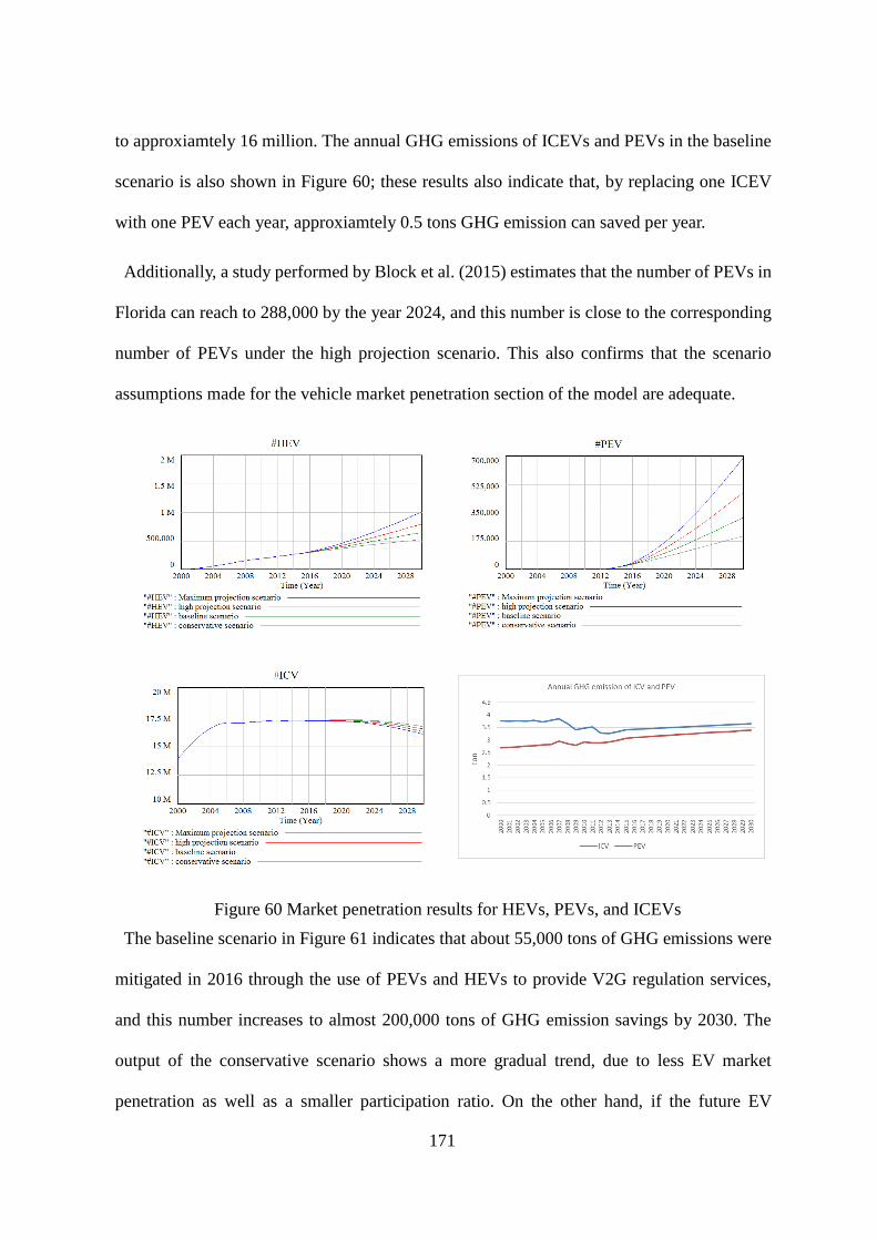
171

to approxiamtely 16 million. The annual GHG emissions of ICEVs and PEVs in the baseline

scenario is also shown in Figure 60; these results also indicate that, by replacing one ICEV

with one PEV each year, approxiamtely 0.5 tons GHG emission can saved per year.

Additionally, a study performed by Block et al. (2015) estimates that the number of PEVs in

Florida can reach to 288,000 by the year 2024, and this number is close to the corresponding

number of PEVs under the high projection scenario. This also confirms that the scenario

assumptions made for the vehicle market penetration section of the model are adequate.

Figure 60 Market penetration results for HEVs, PEVs, and ICEVs

The baseline scenario in Figure 61 indicates that about 55,000 tons of GHG emissions were

mitigated in 2016 through the use of PEVs and HEVs to provide V2G regulation services,

and this number increases to almost 200,000 tons of GHG emission savings by 2030. The

output of the conservative scenario shows a more gradual trend, due to less EV market

penetration as well as a smaller participation ratio. On the other hand, if the future EV

172

adoption rate can reach the maximum projected value and the market can implement a more

sophisticated business mode, a more widely available aggregator, and well-built infrastructure,

the resulting emission savings can be as high as 1.6 million tons.

In addition to mitigating emissions by providing cleaner regulation services, the fundamental

goal of shifting the energy structure away from thermoelectric energy in favor of renewable

energy sources can also be achieved by V2G technology. It can be concluded from the results

in Figure 62 that, by introducing more wind power with the support of the studied V2G system,

the overall emission rate from the power grid can potentially be reduced from 0.68 ton/MWh

to less than 0.55 ton/MWh. This is an important finding with respect to the adoption of V2G

technology because this reduced grid emission rate not only affects the emission rates from

electricity generation alone but also reduces the overall GHG emission rate from the passenger

car sector.

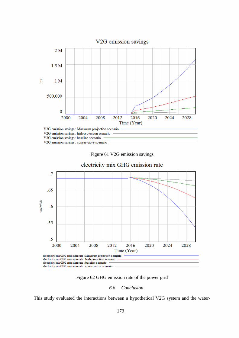
173

Figure 61 V2G emission savings

Figure 62 GHG emission rate of the power grid

6.6 Conclusion

This study evaluated the interactions between a hypothetical V2G system and the water-

174

energy nexus via a combination of the system dynamics modeling approach and the life cycle

assessment method. The underlying complex relationships among the applicable social,

economic, and environmental variables were investigated, and the future development of the

system was predicted accordingly. Four scenarios representing different possible futures for

EV and V2G adoption levels were likewise tested. Some of the important findings from this

study are listed below:

1. V2G technology could be an ideal solution for problems related to the optimization of

the water-energy nexus and for the decarbonization of current electricity grid, as V2G

systems are essentially an aggregation of several idle EV batteries, each of which can

achieve a bidirectional energy transmission with limited modifications and/or investments

from vehicle owners; the additional capacity provided by these batteries can increase the

efficiency of the power grid and accommodate cleaner renewable power sources despite

the inherent intermittency of their power outputs.

2. In addition to lower fuel and maintenance costs, the potential revenue of providing

V2G regulation service may also be appealing to car buyers, making V2G systems a

potentially critical element of a reinforcing feedback loop to facilitate the formation of a

more sustainable system overall, including a larger EV fleet with higher energy

efficiencies and lower tailpipe emissions. Based on the V2G services that can be provided

by this fleet, the efficiency of the grid can also be increased, and more wind power can

therefore be integrated. Subsequently, the newly adopted large-scale wind capacity not

only decreases the emissions of electricity generation and further reduces the life-cycle

emissions of EVs but also consumes less water; the latter in particular leads to less overall

energy consumption within the system.

3. Sophisticated business modes and a good scheduling and controlling mechanism will

175

both be required from system operators, and more importantly, a certain amount of willing

participants among the EV customer base will be essential to ensure an adequate V2G

system. The results under a more conservative scenario indicated that a minimum EV

market share of approximately 10%, combined with an availability/participation ratio for

regulation services of at least 0.5%, would provide sufficient support for large-scale wind

power integration.

4. The results of the simulations in this study indicated that the electrification of the

passenger vehicle fleet will increase the GDP of the passenger car sector, but when

combined with GDP from other sectors, the EV market has a fairly small impact on the

population. Hence, the most effective connection between the environmental and

economic sections of the overall system will be the incentives provided to encourage the

adoption of EVs; in real life, this would most likely be in the form of economic incentives,

such as lower prices for EVs.

5. With all of the relevant life cycle factors taken into consideration, the overall

mitigation potential for GHG emissions was still found to be positively correlated with

the number of EVs and the participation ratios with respect to V2G regulation services.

The result of all four scenarios indicated a certain level of GHG emission mitigation, and

among all of the assumptions made for these four scenarios, increasing wind power

capacity was found to be the most effective way of reducing these emissions from the

system as a whole.

Even though a wide variety of social, economic, and environmental variables have been

investigated and simulated in this study, vehicle configurations and the behavior of the owner

within each vehicle type were still considered within a relatively generic context. To build a

more detailed model that can reflect a person’s decision and the subsequent impacts on the

system, a future study incorporating an agent-based modeling (ABM) approach into the

176

established framework can be performed and thereby analyze the modeled system from a

more realistic perspective.

177

7 THE IMPACT OF VEHICLE-TO-GRID SYSTEM TO THE FUTURE

TRANSPORTATION AND ENERGY SYSTEM – A SYSTEM DYNAMICS

MODELLING APPROACH WITH UNCERTAINTY ANALYSIS

The introduction of clean energy source such as wind or solar power can effectively reduce

the fuel consumption, air emissions and water consumption of the energy system. However,

large-scale clean energy integration requires ancillary services or energy storage capacity to

eliminate the intermittent power output. In this paper electric vehicles are assumed to be the

ancillary service carriers for wind power through Vehicle-to-Grid systems. The connections

and dynamics among electric vehicle adoption, wind power integration, water-energy nexus of

power generation, effects of air emissions to human health, and the economic impacts of

Vehicle-to-Grid technology to vehicle owners are simulated through a system dynamics model.

In addition to the system dynamics model developed from last Section, an uncertainty analysis

is incorporated in this section to address the uncertainties of the studied variables and the

unknown business model or operation details.

7.1 Introduction

Electricity generation and transportation generate the largest and second largest share of

greenhouse gas (GHG) emissions in the U.S. (U.S. Environmental Protection Agency, 2016).

Both sectors rely heavily on fossil fuels, currently more than 80% of U.S. electricity is

generated from fossil fuel or nuclear power, and approximately 90% of the 260 million

registered vehicles are powered by gasoline or diesel. As the economy and population grow,

the increasing commuting needs and poor traffic conditions would further worsen the air

pollution situation, and cause cardiovascular and respiratory issues to urban residents. Other

than air emissions, thermoelectric power plants which generate electric power from petroleum

combustion or nuclear reaction consume significant amount of water for cooling purpose.

178

To increase fuel efficiency, vehicles partially or fully powered by electricity have been

introduced to the market. Hybrid electric vehicles (HEV) capture braking energy and power

utilize it for a certain speed range; some plug-in hybrid electric vehicle (PHEV) models have

larger battery packs and can obtain electric power directly from the grid; the newer plug-in

electric vehicles (PHEV) operate entirely on electric powertrain and are fully independent

from fossil fuel. However, for vehicles using electricity as power source, whether or not air

emissions can really be reduced depends on the percentage of the “clean” power sources in

the energy structure. Electricity is a unique commodity in that it must be generated and

consumed at the same time. So, the electricity market can be generally divided into energy-

related market and power-related market. Electricity in energy-related market is generated by

coal or nuclear power plants at a stable rate. On the other hand, power-related market is

consisted by ancillary services such as regulation service or spinning reserve, and these

services balance the demand and supply and ensure the reliability of the grid. Wind or

photovoltaic power are clean yet intermittent power sources, so comparing with traditional

power generation, wind power plants require more ancillary services to maintain a stable

output.

Vehicle-to-Grid (V2G) system further integrates electricity generation and transportation

sectors by allowing electric vehicles (EV) supplying electricity back to the grid as ancillary

capacity providers. By plugging EVs into the grid, local aggregators can coordinate and

allocate the backup power capacity (in kW or MW) to compensate the fluctuated power output

from wind farms. So, traditional combustion turbines as ancillary service carriers, can be

replaced by the aggregated battery capacity of EVs. Studies have shown that, with a

sophisticated network, commercial fleets (Hill et al., 2012; Zhao et al., 2016a) and private EV

owners (Noori et al., 2016) can gain economic benefits from providing V2G regulation

services. More importantly, the large-scale renewable energy supported by contracted EVs

179

can reduce the emission rate of the entire energy system and further mitigate the carbon

footprint of the transportation sector. In addition, with a higher renewable energy ratio, water

withdrawal and consumption of the energy sector can be mitigated.

As V2G technology connects the electricity generation and transportation sectors, a network

consists of social, environmental, and economic aspects is formed. In this network, elements

from individual scale including vehicle price, operation and maintenance cost, V2G service

revenue, and consumer’s choice, to high-level systems such as GDP, population, GHG

emissions from transportation sector, water consumption from energy structure, and the

integration of wind as energy source interconnect with each other and affect the dynamics of

the network. Therefore in this paper, the transportation-V2G-energy network is simulated by

a system dynamics model; social, environmental, and economic aspects of the model is

represented by GDP/population, GHG/particular matter (PM), and vehicle life cycle cost

respectively. Reinforcing and balancing loops of the systems are identified, and quantitative

relations of all the variables in the model are computed and validated based on historical data.

The uncertainty of critical variables are studied by a sensitivity analysis. The state of Florida

is the study region and the modelling time is from 2000 to 2030. The rest of the study is

categorized in following sessions:

A literate review is conducted in Section 7.2

The main method, the sub-models, and the model verification and validation is

explained in Section 7.3

The results are illustrated and discussed in Section 7.4

The conclusion and findings are summarized in Section 7.5

180

7.2 Literature review

The bulk of the electricity is from the baseload energy market, the baseload electricity is

typically generated from coal or nuclear plants at fairly low cost, however, this type of

generation lacks the ability to alter its output in a short period of time. The other type of

electricity on the energy market is peak power, which typically generated from gas turbine.

Peak power is purchased to cope a seasonal demand peaking. Other than the bulk energy

generation, ancillary regulation service, also known as automatic generation control (AGC)

on the power market is also required to ensure the balance on the grid. In deregulated power

markets, regulation services are commonly provided by independent system operators (ISO)

and regional transmission organizations (RTO). EVs aggregated via V2G system are

promising regulation service providers because of the great potential capacity the future EV

fleet has and the high-efficiency nature of storing and supplying electricity through batteries

(Kempton and Tomić, 2005a). The main advantage of V2G system as regulation service

carrier over traditional gas turbine system to avoid constantly altering the power output of the

gas turbine and mitigate GHG emissions (Lin, 2011). In addition, V2G system is virtually

already exist since the power system is bi-directional, and the implementation of such system

presents great economic value (Kempton et al., 2001). Studies also have shown both

commercial fleets and private EVs can achieve GHG emission reduction and economic

benefits (Noori et al., 2016; Zhao et al., 2016a). The emission source of EVs are mainly in the

electricity generation phase, therefore life cycle assessment (LCA) method combined with

uncertainty analysis has been adopted in V2G studies (Noori et al., 2016; Zhao et al., 2016a).

A study has revealed that significant more backup capacity will be required to accommodate

large-scale wind power output (Korchinski, 2013), yet current energy structure lacks both

storage and transmission ability (Flynn, 2008). In regarding of the integration of V2G and

large-scale wind power, Albadi and El-Saadany (2010) have reached two conclusion, the cost

181

of traditional ancillary services may increase significantly, and fast-responding means such as

energy storage might reduce the operational cost. A study has also be done to consolidate the

quantitative relationships of EVs in a wind power and V2G system (Kempton and Tomić,

2005b). A study conducted by Ekman (2011) also confirmed the feasibility of utilizing V2G

system to provide ancillary regulation service for wind farms. Zhao et al. (2017) analyzed the

environmental impacts of supporting new wind power through V2G systems in various

ISO/RTO regions.

As an important indicator of the scale of the future V2G system, the market penetration of

EVs has been studied. Agent based modelling approaches have been used to simulate

individual potential consumers’ choices (Eppstein et al., 2011) or the interactions between a

group of consumer (Noori and Tatari, 2016). EVs typically have a higher initial cost than that

of internal combustion vehicles (ICV), however, the fuel cost of EVs is lower, and the battery

price is decreasing as technology advances. In addition, federal and most state governments

provide cash incentives or tax credit to EV buyers, which may encourage more potential

buyers to choose EV. A study performed by Jenn et al. (2013) have indicated that, statistically,

gasoline price and government incentives have significant impact to buyers’ choice. Another

study confirmed the significance of gasoline price but argues the incentives’ impacts are not

as high (Diamond, 2009). Based on a survey of consumers’ choices, the study conducted by

Curtin et al. (2009) have summarized that environmental and non-economic factors have

higher influences over economic factors. Other studies have reached conclusions that

charging infrastructure (Sierzchula et al., 2014), financial, and battery-related factors (Krupa

et al., 2014) play important roles in buyers’ decision making.

The water-energy nexus within the electricity generation sector has been studied by (Cooper

and Sehlke, 2012), and their finding is that the mitigation of GHG emission at a system level

also requires changes from economic and social aspects, and the most efficient approaches

182

include incorporating more clean energy and developing vehicles with higher fuel efficiency.

A review study has pointed out that it is critical to identify the underlying improvements in

the water usage of energy generation (Nair et al., 2014). A water-energy nexus research (cite

a literature review) has pointed out that there are great potentials in reducing energy

consumption from water treatment, and the optimization of energy structure is critical to

decrease the consumption of water.

The EV market penetration, social, economic and environmental impacts of renewable

energy integration via a V2G network, and the water-energy nexus within the energy system

have not been studied as a whole, and current literature lacks the uncertainty analysis of the

future energy-transportation system. To this end, a system dynamics model is built to reflect

the quantitative relationships among the single vehicle level variables with system level social,

economic and environmental variables. The goal of this study is to explore the underlying

interconnections and reinforcing and balancing loops of the EV-V2G-wind power network;

and based on the validated model, uncertainties are given to critical parameters (such as

incentive or V2G regulation service price) and the overall future system behavior is explored

and predicted.

7.3 Methods

Exploratory Modeling and Analysis (EMA) is a research approach that uses scenario-based

model to analyze complex and uncertain problems (Kwakkel and Pruyt, 2013). As a future

oriented technology, the specific operation details and business models remain unknown. To

study the system integrated with GDP, population, and air emissions from energy and

transportation sectors, the EMA method is used to construct a system dynamic model and to

answer the following questions:

Will there be sufficient amount of EVs to support large-scale wind power integration?

183

What are the factors that may influence the market penetration of EVs, and will EV

become a favorable option in the future?

Will the economic benefit of V2G system prompt the adoption of EVs?

What would be the GHG and PM emissions of the transportation and energy sector?

What are the impacts of the EV-V2G-wind power network to GDP and population?

Will the V2G system provide the foundations to optimize energy structure?

Will there be positive impacts to the water-energy nexus?

Which variables will have higher influence to the network?

7.3.1 Scope of study, model structure and initial assumptions

The state of Florida is selected as the research region. Florida has the fourth largest economy

in the U.S. with approximately 5% of the overall GDP (U.S. Department of Commerce,

2017a); Florida also has the fourth largest population in the nation, and about 20 million

registered vehicle on the road. As of 2014, natural gas has become the majority of the

electricity sources. Although Florida is currently not one of the deregulated markets where

transmission and generation of electricity are operated by different entities, there’s no physical

obstacle preventing EV owners’ from providing V2G regulation services. The state promotes

EV adoption by exempting high occupancy lane rules for EVs (Florida DMV, 2015) and

provide incentives for purchasing vehicle charging equipment(National Conference of state

Legislatures, 2015). As the electrification of transportation taking place, the infrastructure in

Florida has started to incorporating more features for large-scale electric or autonomous

vehicles in the future (Florida Department of Transportation, 2016).

The system dynamics model in this study is built and utilized in the following steps:

Firstly, the basic logic of the model is preliminary identified based on existing literature. By

identifying a series of reinforcing or balancing effects among the variables, a causal loop

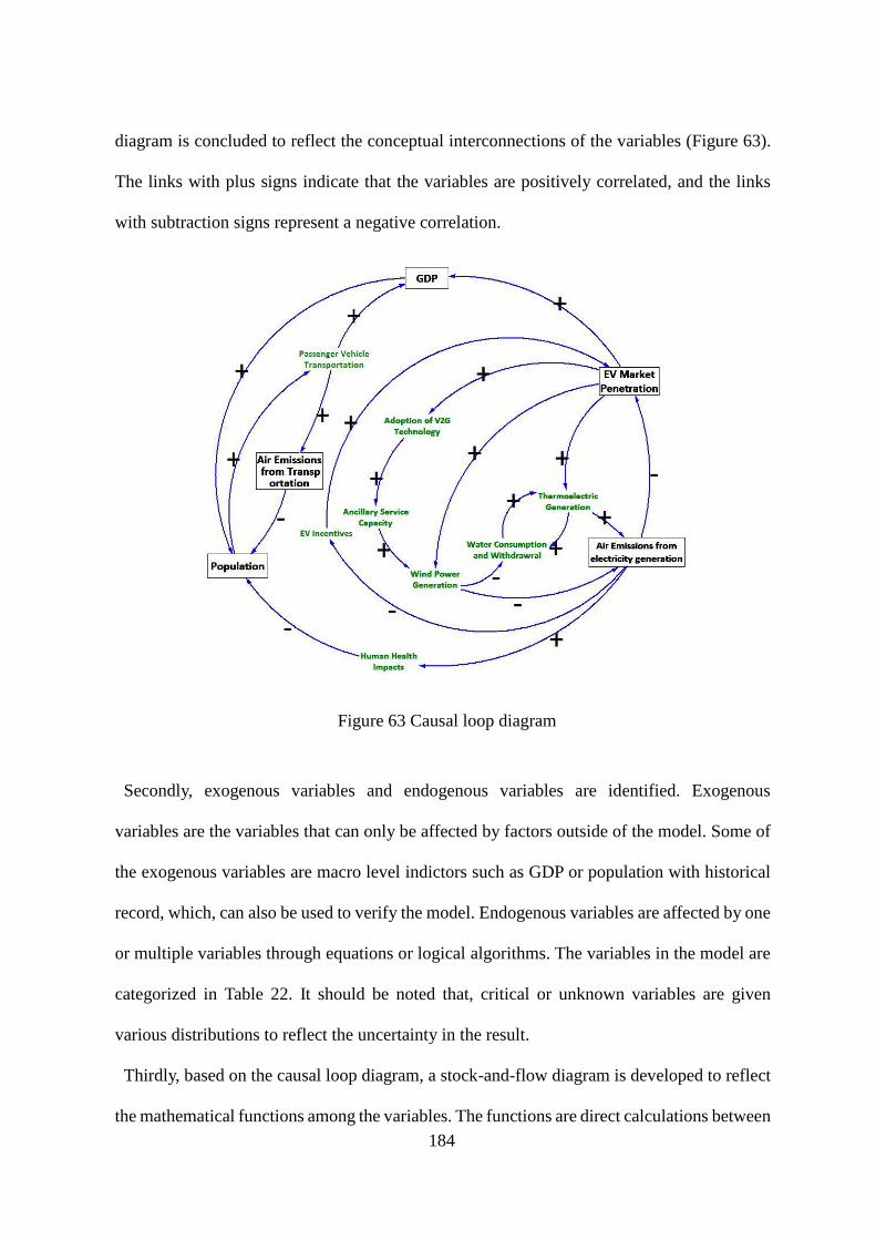
184

diagram is concluded to reflect the conceptual interconnections of the variables (Figure 63).

The links with plus signs indicate that the variables are positively correlated, and the links

with subtraction signs represent a negative correlation.

Figure 63 Causal loop diagram

Secondly, exogenous variables and endogenous variables are identified. Exogenous

variables are the variables that can only be affected by factors outside of the model. Some of

the exogenous variables are macro level indictors such as GDP or population with historical

record, which, can also be used to verify the model. Endogenous variables are affected by one

or multiple variables through equations or logical algorithms. The variables in the model are

categorized in Table 22. It should be noted that, critical or unknown variables are given

various distributions to reflect the uncertainty in the result.

Thirdly, based on the causal loop diagram, a stock-and-flow diagram is developed to reflect

the mathematical functions among the variables. The functions are direct calculations between

185

variables within one sector, i.e. vehicle fuel economy and vehicle annual fuel consumption;

some functions that link different sectors are calculated based on regression of historical data

and then validated, i.e. the economy of vehicle transportation and overall GDP; and there are

also other functions that links micro and macro level variables, i.e. the function that calculate

the potential ancillary service capacity based on individual EV available power output.

Lastly, the model is ran from the year of 2000 to 2030, the results of the first 15 years are

used for model verification and validation, and the possible outcomes of different scenarios

are projected from 2015 to 2030.

186

Table 22 Endogenous and Exogenous variables

Endogenous variables Exogenous variables

Sub-model 1:

Vehicle life

cycle cost and

V2G service

income

annual manufacturing cost of Vehicles manufacturing cost data of Vehicles

annual maintenance and fuel cost of Vehicles maintenance and fuel cost data of

Vehicles

PEV battery degradation multiplier vehicle configuration data of Vehicles

gasoline price increment annual VMT

PEV and HEV available power PEV battery cost

PEV and HEV energy provision/night battery price multiplier

PEV and HEV V2G provision income gasoline and electricity price

PEV and HEV capacity income fuel economy of Vehicles

V2G capacity price

EV plug-in time

Sub-model 2:

GDP,

population, and

vehicle market

penetration

GDP from passenger car transportation GDP from the rest of the sectors

total GDP GDP increasing rate

GDP per capita reproductive lifetime

fertility, maturation and death rate life expectancy

adjusted life expectancy market share of passenger vehicles

population baseline percentage of Vehicles

number of potential drivers

marginal human health impact from

emissions

new passenger vehicle sales

number of HEV, PEV and ICV

V2G promotion effect percentage

mortality rates at various life stage

PEV and HEV incentives

Sub-model 3:

Air emissions

and emission

saving

annual GHG emission of Vehicles average air emission rate before 2015

annual PM emission of Vehicles battery manufacturing air emission rate

electricity mix GHG and PM emission gasoline life cycle GHG emission rate

V2G air emission savings gasoline life cycle PM emission rate

future electricity air emission rate gas turbine GHG and PM emission rate

overall air emission from electricity

consumption

V2G request signal strength

cycle number

Sub-model 4:

Water-energy

nexus

HEV and PEV ancillary service capacity HEV and PEV available power factors

renewable power capacity growth ancillary service requirement ratio

capacity of power sources emission rates of different electricity

sources

annual generation of power sources water withdrawal rates of electricity

sources

saline water withdrawal water evaporation rate

fresh water withdrawal energy intensity ratio of water

treatment

fresh water evaporation renewable generation multiplier

electricity saving of water treatment evaporation rate

fresh water energy intensity ratio

187

The EVs in this study is assumed to be generic, so instead of attribute probability to

indicators, the influence of various factors are interpreted as equations to increase or decrease

the percentage of newly purchased PEVs or HEVs. Since V2G regulation service does not

require deep charging or discharging, both PEVs and HEVs are assumed to be able to connect

to the grid. As the literature shows that V2G ancillary service can be economically appealing

to drivers, it is also assumed that there is a sophisticated service system with aggregators (i.e.

utility companies or vehicle dealers) to gather the power capacity from individual vehicles.

Currently there is limited renewable power capacity in the power system of Florida, the model

is built on the assumption that the newly integrated wind power is supported by the ancillary

service capacity of EVs via V2G system. In the water-energy nexus sub-model, only the water

withdrawal and consumption within the energy generation sector is considered; residential

and irrigation water usage is not included.

Based on the baseline assumptions, the model is divided into several sub-models and

explained through Section 7.3.2 to 7.3.5. The connections of the sub-models are shown in

Figure 64

Figure 64 Sub-models of the system

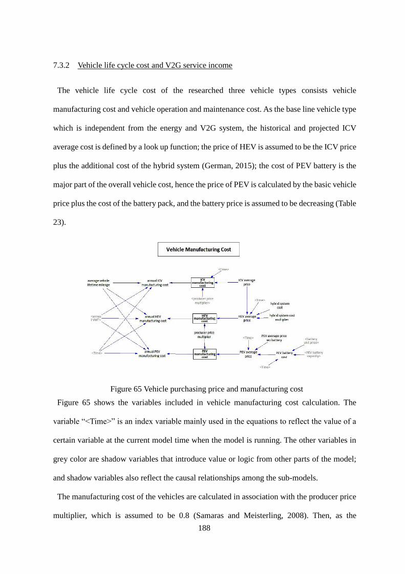
188

7.3.2 Vehicle life cycle cost and V2G service income

The vehicle life cycle cost of the researched three vehicle types consists vehicle

manufacturing cost and vehicle operation and maintenance cost. As the base line vehicle type

which is independent from the energy and V2G system, the historical and projected ICV

average cost is defined by a look up function; the price of HEV is assumed to be the ICV price

plus the additional cost of the hybrid system (German, 2015); the cost of PEV battery is the

major part of the overall vehicle cost, hence the price of PEV is calculated by the basic vehicle

price plus the cost of the battery pack, and the battery price is assumed to be decreasing (Table

23).

Figure 65 Vehicle purchasing price and manufacturing cost

Figure 65 shows the variables included in vehicle manufacturing cost calculation. The

variable “<Time>” is an index variable mainly used in the equations to reflect the value of a

certain variable at the current model time when the model is running. The other variables in

grey color are shadow variables that introduce value or logic from other parts of the model;

and shadow variables also reflect the causal relationships among the sub-models.

The manufacturing cost of the vehicles are calculated in association with the producer price

multiplier, which is assumed to be 0.8 (Samaras and Meisterling, 2008). Then, as the

189

contribution to the GDP of transportation sector, the annual vehicle manufacturing cost is

computed using Equation 30:

𝐴𝑛𝑛𝑢𝑎𝑙 𝑣𝑒ℎ𝑖𝑐𝑙𝑒 𝑚𝑎𝑛𝑢𝑓𝑎𝑐𝑡𝑢𝑟𝑖𝑛𝑔 𝑐𝑜𝑠𝑡𝑗 =𝑉𝑒ℎ𝑖𝑐𝑙𝑒 𝑚𝑎𝑛𝑢𝑓𝑎𝑐𝑡𝑢𝑟𝑖𝑛𝑔 𝑐𝑜𝑠𝑡𝑗×𝐴𝑛𝑛𝑢𝑎𝑙 𝑉𝑀𝑇𝑖

𝑎𝑣𝑒𝑟𝑎𝑔𝑒 𝑣𝑒ℎ𝑖𝑐𝑙𝑒 𝑙𝑖𝑓𝑒𝑡𝑖𝑚𝑒 𝑚𝑖𝑙𝑒𝑎𝑔𝑒 ( 3 0 )

𝐼𝑛𝑑𝑒𝑥𝑒𝑠:

𝑖: 𝑡𝑖𝑚𝑒 𝑖𝑛𝑑𝑒𝑥 (2000 𝑡𝑜 2030)

𝑗: 𝑣𝑒ℎ𝑖𝑐𝑙𝑒 𝑡𝑦𝑝𝑒 𝑖𝑛𝑑𝑒𝑥

The vehicle maintenance and fuel cost, including battery pack replacement cost for PEV, is

calculated based on the annual vehicle mileage travelled (VMT) (Figure 66). The maintenance

and tire cost per mile for HEV and ICV are assumed to be the same since HEVs also have

onboard combustion engines; the unit maintenance cost for PEVs is typically 70% of that of

ICVs considering PEVs have less complex transmission systems (Gallo and Tomic, 2013).

The gasoline and electricity prices are historical and projected data concluded from the

literature. The fuel efficiency of ICV and HEV are also dynamic, increasing gradually as

technology advances in fuel saving. Although the maintenance and fuel cost of PEV might be

lower, the battery replacement of PEV can be a major cost for PEV owners, and V2G

regulation service provision may further accelerate battery degradation. The nature of V2G

regulation service is to respond to the rapid and short-period regulation up (supplying energy

to the grid) and regulation down (storing excessive energy from the grid), and these signals

will only cause shallow charging and discharging of the battery, hence most studies have

concluded that the battery degradation effect of V2G service is minimal (Bishop et al., 2013;

Peterson et al., 2010). In the model, the battery degradation is positively correlated to the

cycle numbers of regulation service a PEV performs per night, and through the “PEV battery

degradation multiplier”, the life time battery replacement is controlled to 1 to 1.5 depending

on the service load. In addition, the battery unit price is assumed to be decreasing, and to

integrate the uncertainty analysis, the variable “battery price multiplier” is used to simulate

190

the level of battery price decrement. The variables with uncertainties are shown in green color

and further discussed in Section 7.3.7.

Figure 66 Vehicle maintenance and fuel cost

The vehicle lifetime cost-related data sources are summarized in Table 23. In addition, the

yearly gasoline price increment is also computed here and linked to the vehicle market

penetration sub-model as a factor that affects HEV and PEV adoption rate.

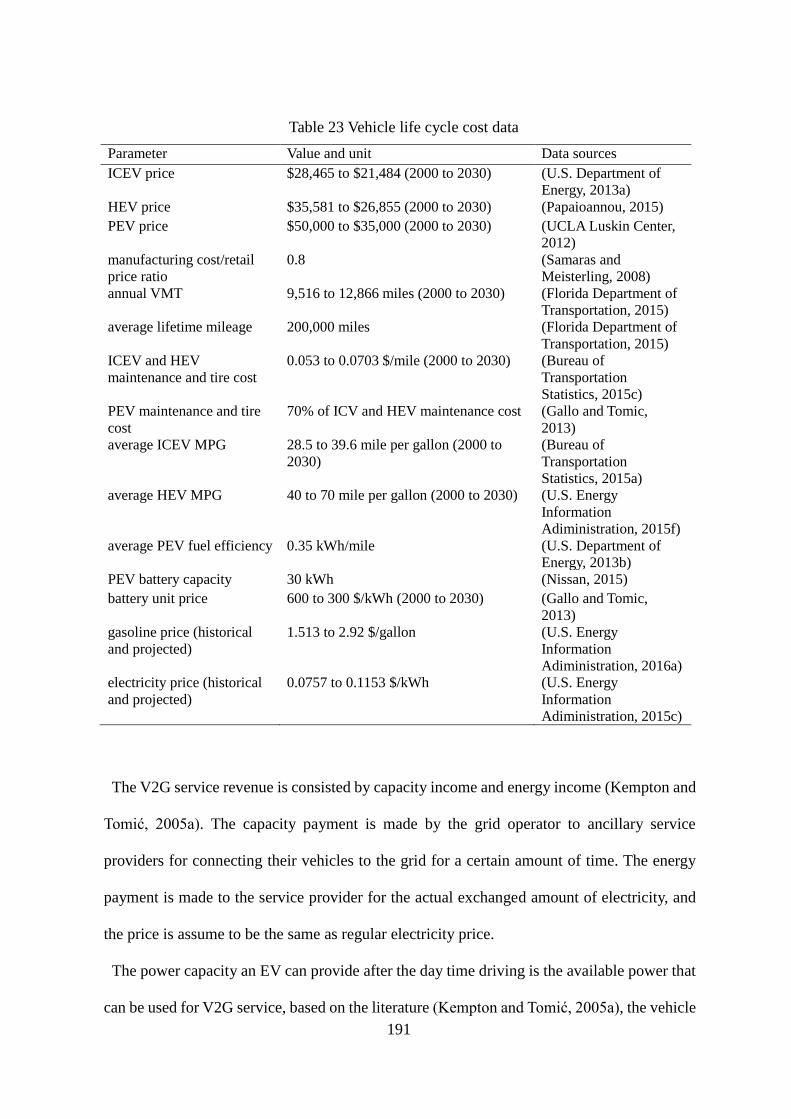
191

Table 23 Vehicle life cycle cost data

Parameter Value and unit Data sources

ICEV price $28,465 to $21,484 (2000 to 2030) (U.S. Department of

Energy, 2013a)

HEV price $35,581 to $26,855 (2000 to 2030) (Papaioannou, 2015)

PEV price $50,000 to $35,000 (2000 to 2030) (UCLA Luskin Center,

2012)

manufacturing cost/retail

price ratio

0.8 (Samaras and

Meisterling, 2008)

annual VMT 9,516 to 12,866 miles (2000 to 2030) (Florida Department of


average lifetime mileage 200,000 miles (Florida Department of


ICEV and HEV

maintenance and tire cost

0.053 to 0.0703 $/mile (2000 to 2030) (Bureau of

Transportation

Statistics, 2015c)

PEV maintenance and tire

cost

70% of ICV and HEV maintenance cost (Gallo and Tomic,

2013)

average ICEV MPG 28.5 to 39.6 mile per gallon (2000 to

2030)

(Bureau of

Transportation

Statistics, 2015a)

average HEV MPG 40 to 70 mile per gallon (2000 to 2030) (U.S. Energy

Information

Adiministration, 2015f)

average PEV fuel efficiency 0.35 kWh/mile (U.S. Department of

Energy, 2013b)

PEV battery capacity 30 kWh (Nissan, 2015)

battery unit price 600 to 300 $/kWh (2000 to 2030) (Gallo and Tomic,

2013)

gasoline price (historical

and projected)

1.513 to 2.92 $/gallon (U.S. Energy

Information


electricity price (historical

and projected)

0.0757 to 0.1153 $/kWh (U.S. Energy

Information

Adiministration, 2015c)

The V2G service revenue is consisted by capacity income and energy income (Kempton and

Tomić, 2005a). The capacity payment is made by the grid operator to ancillary service

providers for connecting their vehicles to the grid for a certain amount of time. The energy

payment is made to the service provider for the actual exchanged amount of electricity, and

the price is assume to be the same as regular electricity price.

The power capacity an EV can provide after the day time driving is the available power that

can be used for V2G service, based on the literature (Kempton and Tomić, 2005a), the vehicle

192

available power of PEV can be calculated by the following equation:

𝐴𝑣𝑎𝑖𝑙𝑎𝑏𝑙𝑒 𝑝𝑜𝑤𝑒𝑟 =𝑏𝑎𝑡𝑡𝑒𝑟𝑦 𝑐𝑎𝑝𝑎𝑐𝑖𝑡𝑦−(

𝑎𝑛𝑛𝑢𝑎𝑙 𝑉𝑀𝑇𝑖365

+𝑏𝑢𝑓𝑓𝑒𝑟𝑖𝑛𝑔 𝑟𝑎𝑛𝑔𝑒𝑖×𝑓𝑢𝑒𝑙 𝑒𝑐𝑜𝑛𝑜𝑚𝑦×𝑐𝑜𝑛𝑣𝑒𝑟𝑠𝑖𝑜𝑛 𝑒𝑓𝑓𝑖𝑐𝑖𝑒𝑛𝑐𝑦)

𝑚𝑎𝑥 𝑑𝑖𝑠𝑝𝑎𝑡𝑐ℎ 𝑡𝑖𝑚𝑒 𝑒𝑎𝑐ℎ 𝑐𝑦𝑐𝑙𝑒( 3 1 )

Where the buffering range is set as 30 miles on average (Kurani et al., 1994) and decreasing

after 2015 as the availability of charging infrastructure increases in the system, and conversion

efficiency is 0.93 (Kempton and Tomić, 2005a). The maximum dispatch time each cycle is

assumed to be 0.3 hour in the literature (Kempton and Tomić, 2005a), and in this model, it is

conservatively set to 0.5 hour for longer dispatching cycles. HEVs, on the other hand,

typically have lower battery capacity yet still consume onboard gas for driving purpose, hence

the available power for HEV is assumed to be 12 kW.

Once vehicle available power is defined, the V2G capacity income can be calculated by

multiplying the available power, EV plug in time, and V2G capacity price (Figure 67). The

plug in time is assume to be 10 hours, and this value is expanded to a range in the uncertainty

analysis. The capacity price can be concluded from wholesale regulation market price

(Shinzaki et al., 2015), so based on previously summarized capacity price in other ISO/RTO

regions (Zhao et al., 2016a), the price is assumed to be $0.03/kWh.

The actual duration of regulation service is obtained by multiplying cycle number and

duration of each cycle. The duration of each cycle is assumed to be 6 minutes (Kempton et

al., 2008). Then, the vehicle energy exchange in kWh is calculated by multiplying vehicle

available power, V2G provision time per night, and the V2G request signal strength, which is

a multiplier for uncertainty analysis. It should be noted here, vehicle plug in time does not

equal to V2G provision time; the former is the time that the vehicle takes to respond to V2G

regulation signal (typically 3.6 to 9 mins each cycle), while the latter is the contracted duration

that the owner connected the vehicle for (usually one night, 8 to 12 hours).

193

Figure 67 Annual V2G service revenue

7.3.3 GDP, population, and vehicle market penetration

The micro level vehicle driving and V2G service providing activities are simulated in

Section 7.3.2, and in this section, the scope of the system is expanded to macro level through

the population amount and percentages of each type of vehicle on the market.

As shown by the stock and flow diagram in Figure 68, the variable “total GDP” is the sum

of “GDP of passenger car transportation” and “GDP from the rest of the sectors”. GDP from

the passenger car transportation summarizes the life cycle cost of each vehicle type and

multiplies with the amount of the vehicle respectively; the GDP from all the other economic

sectors prior to 2015 is reflected by a look-up function of the historical data (Bureau of

Economic and Business Reserve, 2015), and after 2015, the “GDP annual increasing rate”

variable is set to 2.9% based on the GDP growth rate prediction (U.S. Department of

Commerce, 2017a). The per capita GDP is computed by dividing the total GDP by population.

The fertility rate is a deterministic variable for the population model, and the calculation is

shown is Equation 32:

194

𝑓𝑒𝑟𝑡𝑖𝑙𝑖𝑡𝑦 𝑟𝑎𝑡𝑒 = (𝐺𝐷𝑃 𝑝𝑒𝑟 𝑐𝑎𝑝𝑖𝑡𝑎 × 9.57) − (0.233 × 𝑎𝑑𝑗𝑢𝑠𝑡𝑒𝑑 𝑙𝑖𝑓𝑒 𝑒𝑥𝑝𝑒𝑐𝑡𝑎𝑛𝑐𝑦) + 19.97 ( 3 2 )

The adjusted life expectancy is a function that reflects the impact of marginal human health

impact of air emissions to the projected life expectancy (State of Florida Department of Health,

2012). The air emission here includes GHG and PM emissions generated by both

transportation and energy sectors. The verification of this equation is shown in Section 7.3.6.

The adjusted life expectancy also affects the mortality rate of each life stage.

The population mode is a multi-stage stock and flow diagram simulates individuals from

being born and progress through life stages. The births of the population is a function of

fertility rate, population 15 to 44, and reproductive lifetime (assumed to be 30). There are two

important outcomes of the population model, the first is the “population” variable which

influences the “GDP per capita” variable; and the other is the population from 15 to 65 which

consist the potential driver variable.

Figure 68 GDP and population

195

As shown by Figure 69, the new passenger vehicle sales is concluded from the regression of

the historical data of “number of potential drivers”, “GDP per capita”, and “market share of

passenger cars”, the equation is shown below:

𝑛𝑒𝑤 𝑝𝑎𝑠𝑠𝑒𝑛𝑔𝑒𝑟 𝑣𝑒ℎ𝑖𝑐𝑙𝑒 𝑠𝑎𝑙𝑒𝑠 = 𝑚𝑎𝑟𝑘𝑒𝑡 𝑠ℎ𝑎𝑟𝑒 𝑜𝑓 𝑝𝑎𝑠𝑠𝑒𝑛𝑔𝑒𝑟 𝑣𝑒ℎ𝑖𝑐𝑙𝑒 𝑖 ×

(𝐺𝐷𝑃 𝑝𝑒𝑟 𝑐𝑎𝑝𝑖𝑡𝑎×7.3284×107)−(1.2596×𝑛𝑢𝑚𝑏𝑒𝑟 𝑜𝑓 𝑝𝑜𝑡𝑒𝑛𝑡𝑖𝑎𝑙 𝑑𝑟𝑖𝑣𝑒𝑟𝑠)+(3.3242×107)

5 ( 3 3 )

In addition to the potential driver and per capita GDP variables which are derived from the

population and GDP models, the variable “market share of passenger cars” is a look up

function that represents the ratio of passenger cars comparing with all the registered vehicles,

and it is also a look up function varies as model time progresses (Bureau of Transportation

Statistics, 2015b).

Figure 69 Market penetration of HEV, PEV, and ICV

The market penetration of each type of vehicle is calculated as percentages of the overall

new passenger vehicle sales. The percentage of HEV and PEV on the market is affected by

several factors: first, the baseline increasing rate (Block et al., 2015), which is a conservative

rate that reflects the growth of HEV and PEV numbers without the impact of V2G system;

196

second, gasoline price, which is a major factor that affects drivers choice of whether to

purchase an EV or not (Sierzchula et al., 2014), and the correlation is assumed that every 1%

gasoline price increment leads to 1% increase of EV market penetration (Jenn et al., 2013);

third, government incentives (cash or tax credit) also plays important role in the promotion of

EV adoption. Currently there’s no cash incentives in Florida, yet the exemption of HOV rule,

free registration and other discounts can also be considered as promotions. It is assumed that

that will be 4.6% adoption increment per $1,000 incentive (Jenn et al., 2013), and the

uncertainty is also controlled by the “incentive multiplier” variable; fourth, the decreasing

price of EVs can also increase the adoption rate, and based on the literature, per dollar drop

of the price difference between PEV and ICV leads to a 0.5% PEV market penetration

increment (Curtin et al., 2009), and this rate is assumed to be 1% for HEV, identically, the

impact of the maintenance cost is also included, but it may decrease the adoption rate of PEV

since the cost of battery replacement is also included in the maintenance cost. The variables

and their relations are shown in Figure 70.

Figure 70 HEV and PEV market penetration factors

197

7.3.4 Air emissions and V2G emission saving of the system

The air emission and V2G emission saving sub-model includes the annual GHG and PM

emissions generated by passenger cars and electric power generation, and the air emission

saving of the V2G system.

Figure 71 indicates the annual GHG and PM emissions of each type of vehicle. For PEV, the

emissions are mainly generated at the power generation phase. So, in the model, the historical

average grid emission rates are used prior to 2015, and after 2015, the emission rate is dynamic

and correlated to the percentages of each energy source. As an energy intensive process, the

emissions generated by battery manufacturing is also included. To simplify the calculation,

all GHG emissions are converted to CO2, and all traditional air emissions are converted to

PM10.

Figure 71 GHG and PM emissions of HEV, PEV, and ICV

As illustrated by Figure 72, the annual air emissions due to fossil fuel combustion in

transportation sector is summarized by multiplying the GHG or PM emissions of HEVs and

ICVs with the market penetration of the vehicle respectively.

V2G emission savings represents the emissions that are reduced by utilizing the battery of

the EVs to respond the regulation service signals instead of consistently adjusting gas turbines

198

to compensate the fluctuations on the grid. The calculation of V2G GHG emission saving is

shown by Equation 34:

𝐺𝐻𝐺 𝑒𝑚𝑖𝑠𝑠𝑖𝑜𝑛 𝑠𝑎𝑣𝑖𝑛𝑔 = 𝐼𝐹 𝑇𝐻𝐸𝑁 𝐸𝐿𝑆𝐸(𝑇𝑖𝑚𝑒 ≤

2015 , 0,(#𝐻𝐸𝑉×𝐻𝐸𝑉 𝑉2𝐺 𝑒𝑛𝑒𝑟𝑔𝑦 𝑝𝑟𝑜𝑣𝑖𝑠𝑖𝑜𝑛 𝑝𝑒𝑟 𝑛𝑖𝑔ℎ𝑡+#𝑃𝐸𝑉×𝑃𝐸𝑉 𝑉2𝐺 𝑒𝑛𝑒𝑟𝑔𝑦 𝑝𝑟𝑜𝑣𝑖𝑠𝑖𝑜𝑛 𝑝𝑒𝑟 𝑛𝑖𝑔ℎ𝑡)×𝐸𝑉 𝑜𝑤𝑛𝑒𝑟 𝑤𝑖𝑙𝑙𝑖𝑛𝑔𝑛𝑒𝑠𝑠 𝑡𝑜 𝑝𝑎𝑟𝑡𝑖𝑐𝑖𝑝𝑎𝑡𝑒

1000×

𝑎𝑛𝑐𝑖𝑙𝑙𝑎𝑟𝑦 𝑠𝑒𝑟𝑣𝑖𝑐𝑒 𝐺𝐻𝐺 𝑒𝑚𝑖𝑠𝑠𝑖𝑜𝑛 𝑟𝑎𝑡𝑒 × 365) ( 3 4 )

The “If then else” logic ensures the V2G emission saving is zero prior to model time 2015.

After 2015, the low-efficiency energy mitigation is the summation of all the exchanged energy

of HEVs and PEVs during the V2G regulation service provision period. The denominator

1,000 is to convert the unit from kWh to MWh for calculation at the electric grid level. The

ancillary service GHG emission rate is computed by deducting the electricity mix GHG

emission rate by the traditional ancillary service turbine emission rate since the electricity

stored in the vehicle batteries is charged from the grid, and the emission rate of gas turbines

providing ancillary service is typically 2.5 times than that of regular gas turbines (Lin, 2011).

The calculation of V2G PM emission saving follows the same calculation method with PM

emission rate.

Other than the electricity consumed by the newly added EVs, the electricity generation sector

in this sub-model also includes electricity consumptions out of the transportation sector and

the electricity saving due to the integration of wind power. The latter two parts are linked to

the water-energy sub-model. Finally, with all the air emissions summed up, the marginal

human health impact is calculated by multiplying the annual air emissions with GHG and PM

related human health impact factor (Onat et al., 2016a).

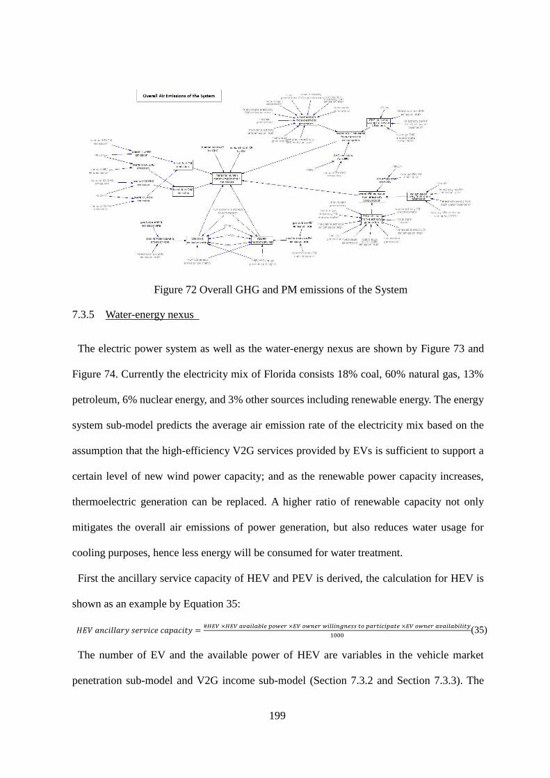
199

Figure 72 Overall GHG and PM emissions of the System

7.3.5 Water-energy nexus

The electric power system as well as the water-energy nexus are shown by Figure 73 and

Figure 74. Currently the electricity mix of Florida consists 18% coal, 60% natural gas, 13%

petroleum, 6% nuclear energy, and 3% other sources including renewable energy. The energy

system sub-model predicts the average air emission rate of the electricity mix based on the

assumption that the high-efficiency V2G services provided by EVs is sufficient to support a

certain level of new wind power capacity; and as the renewable power capacity increases,

thermoelectric generation can be replaced. A higher ratio of renewable capacity not only

mitigates the overall air emissions of power generation, but also reduces water usage for

cooling purposes, hence less energy will be consumed for water treatment.

First the ancillary service capacity of HEV and PEV is derived, the calculation for HEV is

shown as an example by Equation 35:

𝐻𝐸𝑉 𝑎𝑛𝑐𝑖𝑙𝑙𝑎𝑟𝑦 𝑠𝑒𝑟𝑣𝑖𝑐𝑒 𝑐𝑎𝑝𝑎𝑐𝑖𝑡𝑦 =#𝐻𝐸𝑉 ×𝐻𝐸𝑉 𝑎𝑣𝑎𝑖𝑙𝑎𝑏𝑙𝑒 𝑝𝑜𝑤𝑒𝑟 ×𝐸𝑉 𝑜𝑤𝑛𝑒𝑟 𝑤𝑖𝑙𝑙𝑖𝑛𝑔𝑛𝑒𝑠𝑠 𝑡𝑜 𝑝𝑎𝑟𝑡𝑖𝑐𝑖𝑝𝑎𝑡𝑒 ×𝐸𝑉 𝑜𝑤𝑛𝑒𝑟 𝑎𝑣𝑎𝑖𝑙𝑎𝑏𝑖𝑙𝑖𝑡𝑦

1000(35)

The number of EV and the available power of HEV are variables in the vehicle market

penetration sub-model and V2G income sub-model (Section 7.3.2 and Section 7.3.3). The

200

willingness of EV owners participating V2G service is unknown at current stage, so,

uncertainty analysis is also conducted to this variable, and based on the literature, the baseline

value is set as 4% (Parsons et al., 2014). The EV owners’ availability is assumed to be 50%

(Kempton and Tomić, 2005a), meaning half of the participants are available at all time.

In Figure 73, the “ancillary service requirement ratio” (in green color) represents the ratio of

the ancillary service comparing to the new wind capacity. Based on the host area or the scale

of the wind power installation, this ratio may vary from 0.5% to 6% (Kempton and Tomić,

2005b), so, uncertainty analysis is also performed here. With the regulation service capacity

of the passenger car fleet, the annually new wind power capacity that can be supported by

V2G system is derived.

Figure 73 V2G ancillary service capacity and the energy structure

As the EV market penetration varies, the wind power capacity also changes. As is shown by

the links between the variable “renewable capacity growth” with all the other power sources,

it is assumed that the newly integrated renewable power gradually replaces thermoelectric

power sources, and the amount of the capacity of each source being reduced is proportional

to its current percentage in the grid. Based on the historical increasing or decreasing trends,

the annual operation hours of each power source is projected and multiplied with its capacity

201

to obtain the energy generation in MWh. The energy generation of the new wind installation

is unknown, hence a range of 4,000 to 6,000 hours per year is used for uncertainty analysis.

The outcome of the energy system sub-model is the simulation of both historical and future

capacity and generation of each power source, and combining with the GHG and PM emission

rates, the overall electricity mix emission rates are derived and linked to the V2G emission

saving sub-model.

By replacing thermoelectric power sources, wind power generation consumes virtually no

water for cooling. In Florida, surface water are mostly used for electricity generation, and the

majority (93%) of the water consumed is saline water (Scroggs, 2014). Therefore, in the

water-energy sub-model, the replaced thermoelectric power generation is derived from the

energy system sub-model and multiplied with water withdrawal rate of each source to obtain

the amount of water withdrawal mitigated by wind power generation. Depending on the power

source and plant type (once-through or closed loop), the water withdrawal rates vary within

certain ranges, hence uncertainties are also included to these rates, the data are concluded

from the literature (Macknick et al., 2011; Yang and Yamazaki, 2013). The sources of the

water withdrawal is mainly sea water, which leaves 7% of the cooling achieved by utilizing

fresh ground water. Through the variable “evaporation rate” and “fresh water intensity ratio”,

the final outcome of the water-energy nexus sub-model is the mitigated energy consumption

that would otherwise be utilized for water treatment purpose, and the “electricity saving from

fresh water treatment” variable reaches back to the V2G emission saving sub-model.

202

Figure 74 Water-energy Nexus and energy saving

7.3.6 Model validation and verification

Prior to uncertainty analysis, the model is ran with “baseline” or average value given to

uncertainty-related variables, and the model is verified and validated from the following three

angles:

First, the inter-sector equations that derived from regression analysis and include

social or economic influences are verified by plugging in real word data

Second, the output of critical indicators are validated by comparing the model result

prior to 2015 with real-world data

Third, the model is also validated by observing whether the correlation of the variables

comply with initial assumptions

In the GDP and population sub-model, fertility rate is determined by GDP per capita and

adjusted life expectancy; and the parameters of Equation 32 is obtained through a regression

which analyzed the relationship among GDP, life expectancy and fertility rate (with R2=0.67).

203

To verify this equation, the historical GDP data of Florida (Federal Reserve Bank of St. Louis,

2016), the population record (World Population Review, 2015), life expectancy data (Florida

Department of Health, 2015), and the historical fertility data (National Center for Health

Statistics, 2017) are derived from the literature. By plugging in the first three data sets, the

output of Equation 32 is extracted and compared to the real-world fertility data, the

comparison is shown in Figure 75. The ANOVA test indicates there is no significant

differences between the two groups of data.

Figure 75 Fertility equation validation

Similarly, Equation 33 is also derived through a linear regression with the amount of

potential drivers and GDP per capita as independent variables (R2=0.52). The calculation

result is then compared to real-world data of Florida vehicle sales, the result is shown in Figure

76. The ANOVA test indicates there is no significant differences between the two datasets.

2000 2001 2002 2003 2004 2005 2006 2007 2008 2009 2010 2011 2012 2013 2014 2015

Real-world data 2.11 2.10 2.06 2.06 1.96 2.15 2.06 1.97 1.91 1.79 1.88 1.83 1.84 1.83 1.84 1.84

Model calculation 2.15 2.16 1.99 2 2.02 2.06 2.08 2.11 2.05 1.92 1.83 1.8 1.77 1.77 1.77 1.77

0.00

0.50

1.00

1.50

2.00

2.50

Fert

ility

rat

e

Fertility rate: model calcualtion and real-world data

204

Figure 76 Vehicle sales equation validation

In addition to the validation of the equations used for fertility and vehicle sale calculation.

The model output of two macro level indicators: Population and GDP are verified by

comparing to real-world historical data and projections.

Figure 77 shows the extracted population data with baseline assumption and the real-world

population projection (World Population Review, 2015). The result of the ANOVA test is

shown in Table 24, and the F value in of the test is smaller than the F critical value, which

suggests that there is no significant difference between the model output and the real-world

data. It indicates that the population model is relatively accurate.

2000 2001 2002 2003 2004 2005 2006 2007 2008 2009 2010 2011 2012 2013 2014 2015

Model calculation 1.20 1.22 1.25 1.21 1.23 1.31 1.33 1.29 1.14 1.00 1.00 0.98 1.00 1.03 1.07 1.14

Real-world data 1.30 1.28 1.25 1.24 1.26 1.27 1.25 1.20 0.99 0.77 0.86 0.96 1.08 1.16 1.23 1.30

0.00

0.20

0.40

0.60

0.80

1.00

1.20

1.40

Veh

icle

Sal

es (

mill

ion

)Vehicle Sales: model calculation and real-world data

205

Figure 77 Population-model output and real-world data

Table 24 ANOVA test of population


Model 31 627340000

20236774.1

9

2.64961E+

12

Real-world 31

638898994

.7

20609644.9

9

9.28314E+

12

ANOVA Source of


Between

Groups

2.15501E+

12 1

2.15501E+

12

0.36119181

3

0.55010

9

4.00119

1

Within

Groups

3.57982E+

14 60

5.96637E+

12

Total

3.60138E+

14 61

Figure 78 shows the GDP model output and the real-world Florida GDP (Federal Reserve

Bank of St. Louis, 2016; U.S. Department of Commerce, 2017a). The ANOVA test results are

summarized in Table 25, and the smaller F value comparing to F critical value also suggests

that there is no significant differences between the model output and the real-word data. This

0

5,000,000

10,000,000

15,000,000

20,000,000

25,000,000

30,000,000

2000 2005 2010 2015 2020 2025 2030

Population

Model output Real-world data

206

indicates that the assumptions of separating passenger vehicle purchasing and operation cost

from the economic sectors and the calculation of vehicles’ life cycle cost is accurate.

Figure 78 GDP-model output and real-world data

Table 25 ANOVA test of population


Model 31

2980965

0

961601.612

9

7064774320

9

Real-world 31

2799832

6

903171.797

9

6075856831

4

ANOVA

Source of


Between

Groups

5291767079

3 1

5291767079

3

0.80540531

4

0.37306

9

4.00119

1

Within

Groups

3.94219E+1

2 60

6570315576

1

Total

3.99511E+1

2 61

7.4 Results and discussions

The model is first constructed based on variables with average or “most likely” value yet

certain single-value variables may not be able to cover all the possibilities of the system. To

0

200,000

400,000

600,000

800,000

1,000,000

1,200,000

1,400,000

1,600,000

2000 2005 2010 2015 2020 2025 2030

GDP (million $)

Model Real-world

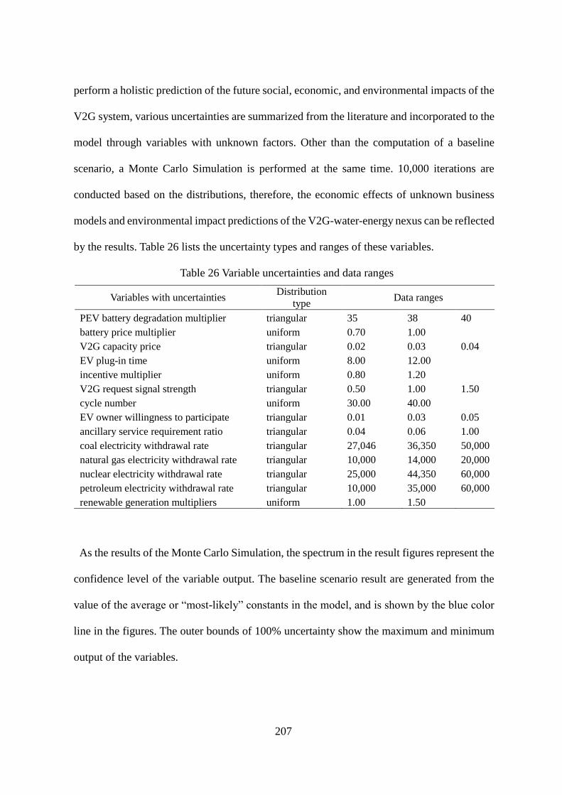
207

perform a holistic prediction of the future social, economic, and environmental impacts of the

V2G system, various uncertainties are summarized from the literature and incorporated to the

model through variables with unknown factors. Other than the computation of a baseline

scenario, a Monte Carlo Simulation is performed at the same time. 10,000 iterations are

conducted based on the distributions, therefore, the economic effects of unknown business

models and environmental impact predictions of the V2G-water-energy nexus can be reflected

by the results. Table 26 lists the uncertainty types and ranges of these variables.

Table 26 Variable uncertainties and data ranges

Variables with uncertainties Distribution

type Data ranges

PEV battery degradation multiplier triangular 35 38 40

battery price multiplier uniform 0.70 1.00 V2G capacity price triangular 0.02 0.03 0.04

EV plug-in time uniform 8.00 12.00 incentive multiplier uniform 0.80 1.20 V2G request signal strength triangular 0.50 1.00 1.50

cycle number uniform 30.00 40.00 EV owner willingness to participate triangular 0.01 0.03 0.05

ancillary service requirement ratio triangular 0.04 0.06 1.00

coal electricity withdrawal rate triangular 27,046 36,350 50,000

natural gas electricity withdrawal rate triangular 10,000 14,000 20,000

nuclear electricity withdrawal rate triangular 25,000 44,350 60,000

petroleum electricity withdrawal rate triangular 10,000 35,000 60,000

renewable generation multipliers uniform 1.00 1.50

As the results of the Monte Carlo Simulation, the spectrum in the result figures represent the

confidence level of the variable output. The baseline scenario result are generated from the

value of the average or “most-likely” constants in the model, and is shown by the blue color

line in the figures. The outer bounds of 100% uncertainty show the maximum and minimum

output of the variables.

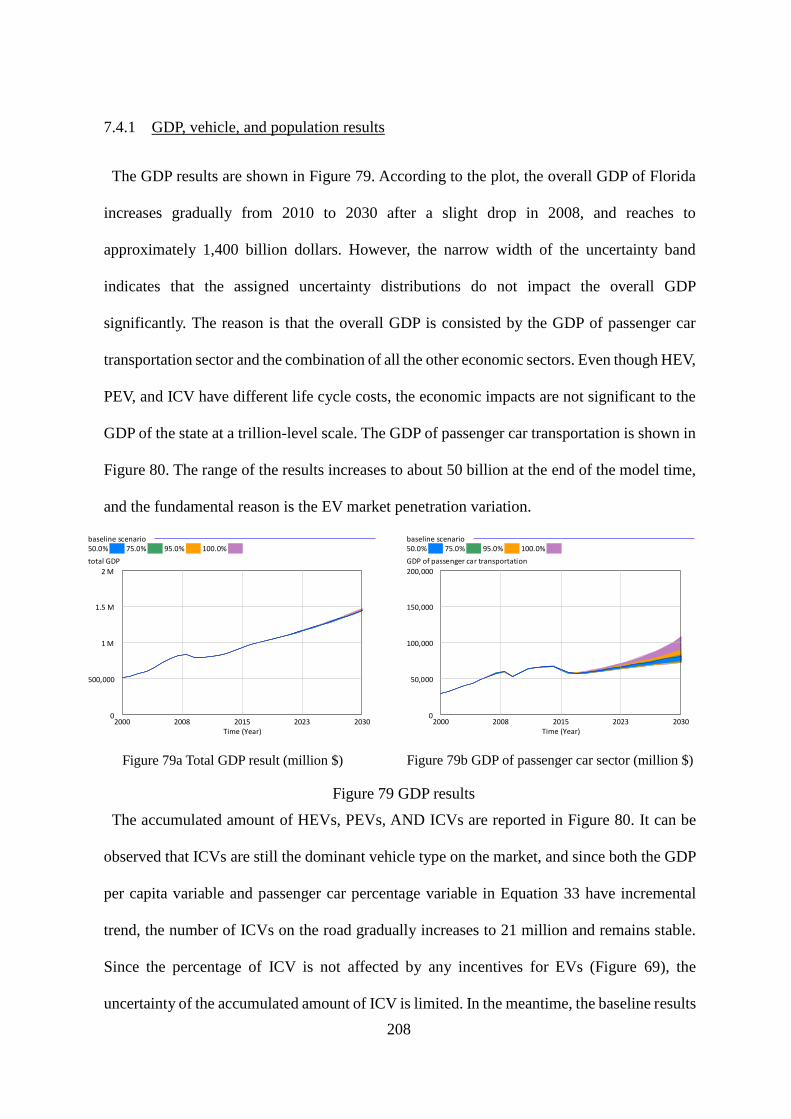
208

7.4.1 GDP, vehicle, and population results

The GDP results are shown in Figure 79. According to the plot, the overall GDP of Florida

increases gradually from 2010 to 2030 after a slight drop in 2008, and reaches to

approximately 1,400 billion dollars. However, the narrow width of the uncertainty band

indicates that the assigned uncertainty distributions do not impact the overall GDP

significantly. The reason is that the overall GDP is consisted by the GDP of passenger car

transportation sector and the combination of all the other economic sectors. Even though HEV,

PEV, and ICV have different life cycle costs, the economic impacts are not significant to the

GDP of the state at a trillion-level scale. The GDP of passenger car transportation is shown in

Figure 80. The range of the results increases to about 50 billion at the end of the model time,

and the fundamental reason is the EV market penetration variation.

Figure 79a Total GDP result (million $)

Figure 79b GDP of passenger car sector (million $)

Figure 79 GDP results

The accumulated amount of HEVs, PEVs, AND ICVs are reported in Figure 80. It can be

observed that ICVs are still the dominant vehicle type on the market, and since both the GDP

per capita variable and passenger car percentage variable in Equation 33 have incremental

trend, the number of ICVs on the road gradually increases to 21 million and remains stable.

Since the percentage of ICV is not affected by any incentives for EVs (Figure 69), the

uncertainty of the accumulated amount of ICV is limited. In the meantime, the baseline results

baseline scenario50.0% 75.0% 95.0% 100.0%

total GDP

2 M

1.5 M

1 M

500,000

02000 2008 2015 2023 2030

Time (Year)


GDP of passenger car transportation

200,000

150,000

100,000

50,000

02000 2008 2015 2023 2030

Time (Year)

209

of HEVs and PEVs indicate that the average number of HEV and PEV reach to 3.48 million

and 3 million respectively in 2030; and the maximum projection can be as high as 8 million

for both vehicle types. In addition, there is a small-scale drop off for both EV type. It is caused

by the assumption that gasoline price has high-influence over the potential buyers’ choice

(Diamond, 2009), and the gasoline market price experienced a major drop down in 2015, and

the functions that convert economic factors to vehicle market penetration is given one year

delay (instead of immediately react to gasoline price or government incentives). Therefore, in

the model time 2016, the low gasoline price has a negative impact to the increment of EV

numbers. As a main factor influencing EV market penetration, Figure 80d depicts the

combined incentive impacts of both gasoline price and government incentives (variables

shown in Figure 70), and the percentage value becomes negative during 2015 to 2017. As

critical components of the vehicle life cycle cost and dependent variables for vehicle market

penetration, the vehicle maintenance and fuel cost comparison are reported in Figure 81. The

annual vehicle maintenance cost of EVs and ICV are shown in Figure 81a. Typically the

maintenance cost of EVs is 70% of average ICV maintenance cost, yet the result indicates

that the annual maintenance cost of PEVs can be approximately $1,400. It is because of the

assumption that the V2G regulation service may cause one or more than one extra battery

replacement, which, may cost as much as $18,000 at the beginning of the model time. The

battery unit price decreases from $600 to $300, hence the overall maintenance cost of PEV

continues to drop after 2015. The battery replacement assumption is a conservative

consideration; because of the much lower life cycle fuel cost (Figure 81b), the market

penetration of EV may increase significantly if one battery is assumed to be sufficient during

the vehicle life cycle. In fact, multiple studies have concluded that V2G regulation services

won’t cause significant battery degradation (Bishop et al., 2013; Peterson et al., 2010). As the

technology of vehicle battery advances and the utilization of second-life battery, it is possible

210

that the market penetration of EVs reach a higher level. Other than the battery replacement

assumption, other assumptions such the government incentives or gasoline price stimulations

are incorporated in the model to reflect the reaction of the market to economic factors, but the

parameters are set at conservative levels based on the literature.

Figure 80a Number of HEV

Figure 80b Number of PEV

Figure 80c Number of ICV

Figure 80d EV incentive impacts

Figure 80 Accumulated vehicle numbers and EV incentive impacts


"#HEV"

8 M

6 M

4 M

2 M

02000 2008 2015 2023 2030

Time (Year)


"#PEV"

8 M

6 M

4 M

2 M

02000 2008 2015 2023 2030

Time (Year)


"#ICV"

30 M

25 M

20 M

15 M

10 M2000 2008 2015 2023 2030

Time (Year)


EV percentage increment

1

.675

.35

.025

-.32000 2008 2015 2023 2030

Time (Year)

211

Figure 81a Maintenance cost comparison

Figure 81b Fuel cost comparison

Figure 81 Vehicle operation cost comparison

The other sub-model affected by the economic sector is the population. The overall

population is determined by a multi-stage stock and flow diagram; and with the input of GDP

per capita variable from the economic sub-model and marginal human impact variable from

the environmental sub-model, the population is projected and shown in Figure 82a. Figure

82b shows the marginal human health impact caused by GHG and conventional air emissions,

the result is dimensionless and reflects the strength of the influence. It can be concluded that

the number of population increased from 17.3 million to 22.7 million gradually even the

marginal health impact varies significantly after 2015. The reason is that the marginal health

impact influences the population sub-model via the variable “adjusted life expectancy”

(Figure 68), where the numeric value shown in Figure 82b is divided by the total number of

population.

Vehicle Annual Maintenance Cost

2000

1500

1000

500

0

2000 2004 2008 2012 2016 2020 2024 2028Time (Year)

do

llar

annual ICV and HEV maintenance and tire cost : baseline scenarioannual PEV maintenance and tire cost : baseline scenario

Vehicle Annual Fuel Cost

2000

1500

1000

500

0

2000 2004 2008 2012 2016 2020 2024 2028Time (Year)

do

llar

HEV annual fuel cost : baseline scenarioICV annual fuel cost : baseline scenarioPEV annual fuel cost : baseline scenario

212

Figure 82a Population

Figure 82b Marginal health impact

Figure 82 Population and health impact results

7.4.2 GHG emission and V2G system results

The overall GHG emission result of the studied system is reported in Figure 83. As

previously illustrated in Figure 72, the overall emission is consisted by the emission from both

passenger car transportation sector and electricity generation sector; and on the other hand,

the operation of V2G system, the overall reduced electricity mix emission rate, and the

decreased water consumption are all factors that contribute to the emission mitigation. As

shown by the figure, the overall GHG emission of the system increases from 142 million ton

in 2000 to 224 million ton in 2015; with the increased adoption of EVs and implementation

of V2G system and wind power generation, the increasing trend of the GHG emission is

changed to decreasing. The baseline scenario indicates that the overall GHG emission can be

reduced to 206 million ton in 2030. In the meantime, the uncertainty spectrum shows that the

maximum emission scenario leads to a rather flat increasing trend at 220 million ton level,

while the minimum emission scenario results in a more drastically decrement to around 175

million ton emission at the end of the model time.


population

30 M

25 M

20 M

15 M

10 M2000 2008 2015 2023 2030

Time (Year)


marginal human health impact from passenger vehicle transportation

400,000

350,000

300,000

250,000

200,0002000 2008 2015 2023 2030

Time (Year)

213

Figure 83 Overall emission (ton)

The average annual GHG emissions of HEV, PEV, and ICV are compared in Figure 84.

Based on the output of the variables, PEV generates the most GHG emissions among all

vehicle types (approximately 6.5 ton per year), and HEV has the lowest annual GHG emission

(approximately 2.4 ton per year). The magnitude as well as the increasing/decreasing trend of

the emission results can be explained by comparing the input variables and assumptions: First,

the GHG emission calculation (Figure 71) includes both upstream (supply) emissions and

downstream (tailpipe) emissions. For vehicles consuming gasoline, both fuel production

phase and tailpipe phase contribute to the overall emission value. For PEV, there is no tailpipe

emission yet the generation of electricity is based on an energy system relies heavily on

thermoelectric power sources (more than 90%). Moreover, the manufacturing of large

capacity battery pack is also environmental-intensive. However, the annual emission of PEV

starts to decrease after 2016, which complies with the percentage change of each power source.

Second, the emission ICV remains stable, because both the fuel economy and annual VMT

assumptions for ICV have limited fluctuation (data sources in Table 23). Third, HEV shows


overall GHG emission

300 M

250 M

200 M

150 M

100 M2000 2008 2015 2023 2030

Time (Year)

214

the best emission performance due to the assumption that the future HEV may have a fuel

efficiency of 70 MPG yet no need to replace large capacity battery pack.

Figure 84 Vehicle GHG emission comparison

The GHG emissions of the entire passenger car sector, GHG emissions of the electricity

generation sector, emission savings from V2G service, and emission savings from reduced

water consumption are summarized in Figure 85. The GHG emissions from the passenger car

sector keeps increasing after 2015 (Figure 85a). Although part of the passenger car fleets is

replaced by HEVs the baseline value indicates the emission reaches to about 83 million ton

in 2030; the reason is the continuous growing overall vehicle number and the increasing

annual VMT. The upstream phase GHG emission of PEVs is allocated to the overall emission

from electricity generation sector (Figure 85b); due to the increasing ratio of wind power

integration, the overall emission from the generation of electricity actually decreases even

part of the energy consumption of the transportation need is shifted to the electricity sector.

This also means that although the life cycle GHG emission of PEVs is higher than that of

HEVs and ICVs, the overall GHG emission in the system can still be mitigated as long as the

electricity mix contains certain percentage of renewable power. Comparing to the overall

Vehicle Annual GHG Emissions

7

5.25

3.5

1.75

0

2000 2004 2008 2012 2016 2020 2024 2028Time (Year)

ton

annual HEV GHG emission : baseline scenarioannual ICV GHG emission : baseline scenarioannual PEV GHG emission : baseline scenario

215

GHG emissions in the system which is around 200 million ton per year, the emission savings

achieved through V2G system can be as high as 20 million ton per year (Figure 85c), mainly

by replacing the low efficiency ancillary gas turbines; and the slightly drop around 2016 is

also due to the changes of EV market penetration. Finally, since wind power generation

requires virtually no water for cooling purpose, the replaced thermoelectric power generation

also leads to less water withdrawal and therefore less water evaporation and consumption;

also, as energy is required to purify such amount of water which could be used for other

purposes, the amount of the energy saved from water treatment is reflected in Figure 85d.

More than 50,000 ton GHG emission can be mitigated in the year of 2030.

216

Figure 85a Overall emission from HEV and

ICV

Figure 85b Overall emission from electricity

generation

Figure 85c V2G emission saving

Figure 85d emission saving from water-energy nexus

Figure 85 GHG emissions and emission savings of transportation and electricity generation

sector (ton)

One of the critical question regarding the implementation of V2G system is whether the EV

number is sufficient to provide a sufficient ancillary service potential. The method of

calculating the available power of a single vehicle for V2G regulation service is discussed in

Section 7.3.2 and Figure 67. The results of the total available power of the passenger car fleet

as well as the potential revenue for EV owner through V2G regulation service is provided in

Figure 86. As shown by Figure 86a, the total regulation service capacity fluctuated slightly

after 2015 and gradually increases to about 2,000 MW, and the maximum scenario might even

reach 9,000 MW; and since the ancillary service-power capacity ratio of wind power is

typically 6%, meaning that more than 30,000 MW wind power can potentially be integrated


fossil fuel GHG emission

100 M

87.5 M

75 M

62.5 M

50 M2000 2008 2015 2023 2030

Time (Year)


overall GHG emission from electricity consumption

200 M

172.5 M

145 M

117.5 M

90 M2000 2008 2015 2023 2030

Time (Year)


V2G GHG emission saving

30 M

22.5 M

15 M

7.5 M

02000 2008 2015 2023 2030

Time (Year)


GHG emission saving from water treatment

90,000

67,500

45,000

22,500

02000 2008 2015 2023 2030

Time (Year)

217

to the grid in 2030. The output of the V2G income variable is also closely related to the

available power of an individual EV. The revenue output of PEV is shown in Figure 86b. It

can be concluded that the revenue of providing V2G service after 2015 is mora than $3,000

per year; and based on Equation 31, this revenue rate is sensitive to the capacity of the battery,

the EV owners’ buffering range decision, EV plug-in duration, and, mostly importantly, the

regulation up/down signal strength. So, from the perspective of the entire transportation-

energy system: a more sophisticated charging infrastructure system will lead to less range

anxiety and more power reservation for V2G service; the more the energy system relies on

V2G system, the stronger the regulation request signals, and hence more revenue for

participants; the large-scale participants will stimulate the EV production, thus lower vehicle

or battery price and more EV buyers; at last, a robust EV market will be able to support more

renewable energy and reduce the environmental impact of driving an EV.

Figure 86a Total ancillary service capacity

(MW)

Figure 86b Potential revenue ($)

Figure 86 Total ancillary service capacity and potential revenue

The energy system outputs are reported in Figure 87. Due to the integration of new wind

power supported by the V2G system, the average electricity mix emission rate declines from

0.8 to 0.5 ton/MWh (Figure 87a), and the uncertainty analysis shows this rate can be as low

as 0.2 ton/MWh. Also, the generation projection is assumed based on historical running time


HEV and PEV ancillary service capacity

10,000

7500

5000

2500

02000 2008 2015 2023 2030

Time (Year)


PEV V2G provision income

6000

4500

3000

1500

02000 2008 2015 2023 2030

Time (Year)

218

of each type of power facility, the projected generation rates are provided in Figure 87b; and

at the end of the model time, about 83 million MWh electricity can be generated through wind

farms, which, will significantly optimize the structure of the V2G-water-energy system.

Figure 87a Electricity mix emission rate

(ton/MWh)

Figure 87b Electricity source generation comparison

(MWh)

Figure 87 Electricity mix results

7.5 Conclusions

This study evaluated the environmental, economic and social interactions within a future

transportation and power generation network connected by V2G system. A system dynamic

modelling approach is used to identify and reflect underlying relationships and causal loops

among critical variables such as population, GDP, vehicle market penetration, GHG emission,

water consumption, wind power, and the V2G system. The model is simulated for 30 years,

the results of the first 15 years is validated with historical data while the output of the last 15

years is explored as a projection for the future system. Due to the unknown operation pattern

of the future V2G system, an uncertainty analysis is incorporated to the model, and the results

are shown with various confidence level to indicate the quantitative result and test the

feasibility of each link of the system.

By constructing the system dynamics model and interpreting the simulation results, the


future electricity GHG emission rate

.8

.6

.4

.2

02000 2008 2015 2023 2030

Time (Year)

Electricity Generation Projection

200 M

150 M

100 M

50 M

0

2000 2004 2008 2012 2016 2020 2024 2028Time (Year)

coal generation : baseline scenarionatural gas generation : baseline scenarionuclear generation : baseline scenariopetroleum generation : baseline scenariorenewable generation : baseline scenario

219

questions raised at the beginning of the study are answered:

Electric vehicles including PEVs and HEVs can be a feasible energy storage solution for

increasing the ancillary service capacity of the energy system. The result indicates

approximately 20% EV ratio can support 30% of the electricity system to be wind power.

However, the electrification of the passenger car fleet cannot impact the GDP and population

sector significantly.

V2G system can reduce the overall emission of the transportation-energy network by

replacing low-efficiency gas turbines, supporting newly integrated wind power, and reducing

the water consumption within the energy system. Based on relatively conservative

assumptions, the total emission savings can be as high as 10 million ton per year; and the

higher ratio of wind power in the electricity grid is the fundamental change of the network.

Government incentives and lower battery unit price are the two most influential factors that

affect the adoption of EVs; the annual income from V2G regulation service can be appealing

to potential vehicle buyers. Hence a sophisticated EV infrastructure with V2G service

aggregators, the reduction of the battery unit price and environmental footprint will facilitate

the implementation of the V2G system.

All the aforementioned results combined together is the most important finding of this study,

a system with reinforcing loops that have positive impacts to environment, economy and

society. The increasing EV adoption rate and the progressing roadway or parking

infrastructure provides an opportunity to implement V2G system; with a much higher

ancillary capacity, the grid is able to integrate more clean energy source; the optimized

electricity mix reduces the life cycle environmental footprint of an EV, and the economic

benefits of V2G service provision also further facilitates the electrification of the

transportation system; finally, the EV or new travelling mode, either autonomous vehicle or

220

vehicle share, provide a robust foundation for the further decarbonization, and ultimately, a

fully developed smart transportation and energy sector.

221

8 CONCLUSIONS

Based on the analysis in Chapter 2, it can be concluded that due to the special driving patterns

and the heavy populated operation areas of parcel delivery trucks, the frequent acceleration and

deceleration as well as long idling times lead to considerably lower fuel efficiency. Problems

related to these driving patterns might be solved by the adoption of battery electric trucks,

which have higher fuel efficiency during low speed driving, and also, the simpler motor and

transmission system makes vehicle maintenance easier and cheaper. With all these advantages,

electric delivery trucks are becoming a very competitive alternative for fleet owners. However,

despite the complete absence of tailpipe emissions, the environmental impacts generated during

other life cycle phases of an electric truck might suggest the opposite. To tackle this issue, the

life cycle GHG emission and energy consumption of diesel, hybrid, CNG and two types of

battery electric trucks have been evaluated by an economic input-output based hybrid life cycle

assessment. And instead of using single value, the uncertainties of key parameters such as the

vehicle manufacturing cost, fuel economy and high capacity battery manufacturing impacts

have been integrated through a Monte Carlo Simulation. In addition, a regional GHG emission

analysis has also been performed based on the adjusted payload factors.

Despite the zero tailpipe emission of electric delivery trucks as opposed to delivery trucks of

other fuel type, electric trucks do not show lower environmental impacts as expected. The

national evaluation indicates that the class 3 electric truck has similar and even slightly larger

life cycle GHG emissions and energy consumption comparing to the diesel, hybrid or CNG

truck. The life cycle CO2-equivalent GHG emission of the aforementioned four types of

vehicle vary approximately from 160 ton to 200 ton, the class 5 electric truck, due to its higher

payload, has higher emission rate, which is about 400 ton. The overall energy consumption of

the diesel and the hybrid truck are less than 2.5 TJ, while that of the CNG and the class 3

222

electric truck is around 4 TJ. It can also be concluded from the result that the majority of

environmental impacts of electric trucks are generated at the electricity generation phase,

meaning that the impacts are moved from downstream to upstream. Therefore, the adoption of

electric truck will not be able to mitigate GHG emission level until more high-emission-rate

power sources are replaced by cleaner power sources.

The regional analysis in Chapter 2 shows that, in regions where electricity generation depends

heavily on coal burning, electric trucks have significantly more GHG emissions than those of

diesel or CNG powered trucks. And the electric vehicle GHG emission saving potential can

only be shown in regions that have large share of cleaner energy as their main electricity

sources. Therefore, it can be concluded that there is a strong relation between the local

electricity generation source and the applicable degree of electric trucks in commercial delivery

truck fleets. Since the year 2000, however, the use of coal as the largest electricity source in

the US has been decreasing continuously, while the use of natural gas and other sources like

wind and solar has been increasing. Therefore, with continuing changes in electric grid

structure and lower manufacturing and retailing prices of electric vehicles due to future

technological improvement, electric trucks may have greater applicability in the future.

This study in Chapter 3 quantitatively compares the GHG emissions of EREVs and BEVs

from a life cycle perspective with and without the use of V2G regulation services, with three

battery wear-out scenarios assumed, analyzed and interpreted to account for uncertainties

related to various degrees of battery wear-out. To address the uncertainties pertaining to

regulation response times, a Monte Carlo Simulation is integrated along with an analysis of

relevant historical data. The results shows that EREVs and BEVs are both viable regulation

service providers for saving GHG emissions from electricity generation if the battery wear-out

from regulation services is assumed to be minimal, but the V2G system becomes less attractive

at higher battery degradation levels.

223

Based on the uncertainty analysis conducted in Chapter 3, it is also observed that the

electricity emission savings with the V2G system are sensitive to regulation signal frequency

and strength, and the total regulation values while providing V2G regulation services are

likewise positively correlated with the emission savings. However, it must also be noted that,

once V2G system is implemented, more electric power exchanges will take place, and more

electricity generation emissions will be avoided as a result. In conclusion, based on the overall

battery degradation levels, ancillary service profits, environmental merits, and future battery

price considerations, regulation/ancillary services are a promising future application for V2G

technology.

However, the widespread implementation of EV and V2G system may face obstacles from

different angles. Firstly, the initial cost of EVs are significantly higher than traditional vehicles

(i.e. the price of the researched BEV is $150,000, which is two times higher than a diesel truck).

Secondly, the lack of EV charging infrastructure may cause the “range anxiety” and prevent

potential customers from purchasing EVs. Thirdly, a sociological research revealed that drivers

seldom consider fuel cost as an important household expenditure and alternative fuel vehicles

ae often related to “low quality” or “cheap” and resisted by customers (Turton and Moura,

2008). Furthermore, the aggressive driving behavior; rural and urban community conflicts due

to moving environmental impact from the city to suburban traditional/renewable power

facilities and impediments from petroleum companies can all obstruct the integration of the EV

and electricity system (Sovacool and Hirsh, 2009). Electric delivery trucks, on the other hand,

are immune to some of the aforementioned problems. For instance: In order to promote clean

delivery trucks, state of New York (New York State Department of Transportation et al., 2015)

and State of California (California Environmental Protection Agency, 2015) initiated “first

come-first served” electric truck incentive programs, which provide $50,000 and $60,000

incentives respectively as well as tax exemptions for EV fleet owners. Delivery trucks operate

224

on a fixed routine and therefore the driver has no range anxiety. And from the perspective of a

fleet operator, when purchasing a new vehicle, the fuel economy and the GHG emission will

be first priorities instead of the shape, color and interior comfortability of the truck. Moreover,

the acceleration or top speed can also be regulated by the fleet operator to optimize the

efficiency of the electric truck. In conclusion, in spite of the obstacles, commercial delivery

fleets can be the first step of a mature V2G system.

The conclusions of the V2G systems, V2G-wind power, and V2G with the transportation-

water-energy network (Chapter 4 to Chapter 7) are summarized below:

While electric passenger car owners as V2G service providers require aggregators to

operate and coordinate due to the low battery capacity and scattered locations of

passenger vehicles, electric delivery truck fleets have inherent advantages as the

preliminary application of V2G technologies, particularly since a fleet with 30 trucks or

above is able to sign contracts with electric grid operators, a delivery truck typically parks

10 to 12 hours a day, and the centralized coordination and fixed routes of standard truck

operation can help to ensure the contractual capacity of the fleet.

For BEVs in the PJM, NYISO, and CAISO regions, a significant total ownership cost

reduction can be achieved by providing V2G regulation services. In areas where

regulation service prices are high, such as the NYISO region, the lifetime V2G regulation

service revenue could even reach as much as $60,000, which leads to a considerably large

amount of profit compared to the initial cost of the EVs.

The total ownership costs of BEVs are significantly lower in the NYISO and CAISO

regions, because the state governments in these two regions are currently promoting the

adoption of electric trucks with a large amount of incentives. However, these funds are

not unlimited and are provided on a first-come-first-serve basis, so as the electrification

225

of truck fleets in these two areas continues, the availability of incentives and the total

ownership costs of electric trucks will inevitably be altered in the future.

For EREVs, the total ownership cost reductions due to regulation services are only

significant in the PJM and NYISO regions, where the revenues are approximately

$20,000 to $30,000 more than the total life cycle ownership cost. However, this is still

profitable given the relatively lower purchasing price of EREVs as opposed to BEVs.

Based on the calculated revenues of each type of vehicle in each region, apart from the

power output availability of the vehicle, the capacity payment revenues of electricity

regulation services will play a crucial role in the net revenue of V2G services, and EVs

in high regulation-capacity-price regions (such as the PJM or NYISO regions) will tend

to have higher V2G service revenues.

Compared to the average net revenue from V2G regulation services, the initial equipment

grid-accessibility upgrade cost (excluding the cost of the EVs themselves) are relatively

small and can typically be repaid in full within the first year.

V2G regulation services are more profitable in regions where the grid is highly fluctuated.

The more electricity processed by the V2G system, the more GHG emissions are reduced,

as the emissions from less efficient gas turbine generators will be mitigated while V2G

service providers receive more revenue.

Even though EREVs have lower battery capacities than BEVs and therefore cannot

provide as much to the grid, EREVs are still able to meet regulation service demand levels.

However, the larger battery capacity of BEVs means that fewer BEVs are needed to meet

the same regulation contract requirement, leading to a more flexible operation schedule

for a BEV fleet than for an EREV fleet.

226

In addition to economic benefits for fleet operators, the use of the V2G system with

delivery truck fleets is proven to have significant GHG emission mitigation effects. On

average a BEV or EREV in each researched region could save approximately 300 tons of

GHG emissions. The GHG emissions of BEVs are mainly generated at electricity

generation and transmission phases, but the life cycle GHG emission savings from

providing V2G services could offset all of the electricity-related or petroleum-related

emissions, as shown in Figure 37. In other words, by integrating EVs into the grid, “zero”

or even “negative” net GHG emissions could be achieved. Furthermore, more savings

will be available for fleet owners once carbon taxes are introduced.

Although BEVs have proven to be more profitable in terms of V2G service revenue,

BEVs did not achieve any significantly greater emission savings than EREVs when V2G

regulation services were considered (Figure 36). This is because, despite the higher power

availability of BEVs, this power availability could not be fully utilized based on the grid

fluctuation balancing demand researched in this study, while the batteries of BEVs are

twice as large as that of EREVs, meaning that each battery replacement for BEVs would

result in a larger GHG impact.

Whether or not the emission savings potential of the V2G-wind power system can be

fully achieved depends heavily on the availability of EVs as V2G regulation providers.

For instance, in the MISO and ERCOT regions, where wind power projections are

considerably higher, the overall emission savings are lower because of the limited EV

population relative to the required number of EVs to meet the regulation demand.

The marginal emissions due to unregulated charging could not outweigh the emission

savings of V2G services in most cases. For example, in the average-case scenario, the

projection wind power integration in the CAISO region is only one-third of the

227

corresponding projection in the MISO region, but the CAISO region still yields a much

larger overall amount of emission savings comparing to the MISO region due to the larger

amount of EVs available in the CAISO region to meet the V2G regulation demand from

increased wind power integration.

The marginal emissions may still offset the environmental benefits of the V2G system

when EVs are adopted on a sufficiently massive scale in a particular region with

unregulated charging schedules, and/or when the region’s regulation requirements are

limited. Hence, the balance between EV projections and wind power projections in any

given region is crucial, especially in regions where a significant degree of wind power

integration is expected, in which case the adoption of EVs and V2G systems should be

promoted to reduce the overall carbon emissions from both sectors.

Once a V2G-wind power system has been properly established in a particular region,

more electricity is exchanged through the system as the regulation requirement signals

become stronger, allowing more additional energy to be saved or given back to the grid.

The results of Chapter 5 indicates that wind power aggregation could effectively mitigate

the variability of the system as a whole and thus reduce the ancillary service burdens

among individual participants, making this aggregation a promising solution for regions

where the projected ancillary service requirements for wind power integration are high

while EV market penetration is low.

V2G technology could be an ideal solution for problems related to the optimization of

the water-energy nexus and for the decarbonization of current electricity grid, as V2G

systems are essentially an aggregation of several idle EV batteries, each of which can

achieve a bidirectional energy transmission with limited modifications and/or

investments from vehicle owners; the additional capacity provided by these batteries can

228

increase the efficiency of the power grid and accommodate cleaner renewable power

sources despite the inherent intermittency of their power outputs.

In addition to lower fuel and maintenance costs, the potential revenue of providing V2G

regulation service may also be appealing to car buyers, making V2G systems a potentially

critical element of a reinforcing feedback loop to facilitate the formation of a more

sustainable system overall, including a larger EV fleet with higher energy efficiencies and

lower tailpipe emissions. Based on the V2G services that can be provided by this fleet,

the efficiency of the grid can also be increased, and more wind power can therefore be

integrated. Subsequently, the newly adopted large-scale wind capacity not only decreases

the emissions of electricity generation and further reduces the life-cycle emissions of EVs

but also consumes less water; the latter in particular leads to less overall energy

consumption within the system.

Sophisticated business modes and a good scheduling and controlling mechanism will

both be required from system operators, and more importantly, a certain amount of

willing participants among the EV customer base will be essential to ensure an adequate

V2G system. The results under a more conservative scenario indicated that a minimum

EV market share of approximately 10%, combined with an availability/participation ratio

for regulation services of at least 0.5%, would provide sufficient support for large-scale

wind power integration.

The results of the simulations in this study indicated that the electrification of the

passenger vehicle fleet will increase the GDP of the passenger car sector, but when

combined with GDP from other sectors, the EV market has a fairly small impact on the

population. Hence, the most effective connection between the environmental and

economic sections of the overall system will be the incentives provided to encourage the

229

adoption of EVs; in real life, this would most likely be in the form of economic incentives,

such as lower prices for EVs.

With all of the relevant life cycle factors taken into consideration, the overall mitigation

potential for GHG emissions was still found to be positively correlated with the number

of EVs and the participation ratios with respect to V2G regulation services. The result of

all four scenarios indicated a certain level of GHG emission mitigation, and among all of

the assumptions made for these four scenarios, increasing wind power capacity was found

to be the most effective way of reducing these emissions from the system as a whole.

The result in Chapter 7 indicates approximately 20% EV ratio can support 30% of the

electricity system to be wind power. However, the electrification of the passenger car

fleet cannot impact the GDP and population sector significantly.

V2G system can reduce the overall emission of the transportation-energy network by

replacing low-efficiency gas turbines, supporting newly integrated wind power, and

reducing the water consumption within the energy system. Based on relatively

conservative assumptions, the total emission savings can be as high as 10 million ton per

year; and the higher ratio of wind power in the electricity grid is the fundamental change

of the network.

Government incentives and lower battery unit price are the two most influential factors

that affect the adoption of EVs; the annual income from V2G regulation service can be

appealing to potential vehicle buyers. Hence a sophisticated EV infrastructure with V2G

service aggregators, the reduction of the battery unit price and environmental footprint

will facilitate the implementation of the V2G system

230

REFERENCES

AFLEET, 2013. Alternative Fuel Life-Cycle Environmental and Economic

Transportation:2013.

Al-Deek, H., Consoli, F., Rogers, J., Tatari, O., Alomari, A., Sandt, A., 2014. Applications of

Transit Signal Priority for Transit Service,” Final Report, National Center for Transportation

Systems Productivity and Management. Contract #DTRT12GUTC12.

Albadi, M., El-Saadany, E., 2010. Overview of wind power intermittency impacts on power

systems. Electric Power Systems Research 80, 627-632.

Alternative Fuel Data Center. U.S. Plug-in Electric Vehicle Sales by Model.2015. See also:

http://www.afdc.energy.gov/data/10567

Amarakoon, S., Smith, J., Segal, B., 2013. Application of life-cycle assessment to nanoscale

technology: Lithium-ion batteries for electric vehicles.

Anylogic, 2015. Anylogic, 7.3 (Multimethod Simulation Software).

Argonne National Laboratory. The Greenhouse Gas, Regulated Emissions, and Energy Use

in Transportation (GREET) Model: 1-2013.2013. See also: https://greet.es.anl.gov/

Argonne National Laboratory. The Greenhouse Gases, Regulated Emissions, and Energy

Use in Transportation Model 2015. See also: https://greet.es.anl.gov/

Argonne National Laboratory. Alternative Fuel Life-Cycle Environmental and Economic

Transportation (AFLEET).2016. See also: https://greet.es.anl.gov/afleet

Bankrate. CD Investment Rates Results 2014. See also:

http://www.bankrate.com/funnel/cd-investments/cd-investment-

results.aspx?&prods=15&local=false

Barnitt, R.A., Brooker, A.D., Ramroth, L., 2010. Model-based analysis of electric drive

options for medium-duty parcel delivery vehicles.

Bilec, M., Ries, R., Matthews, H.S., Sharrard, A.L., 2006. Example of a hybrid life-cycle

assessment of construction processes. Journal of Infrastructure Systems 12, 207-215.

Bird, L., Lew, D., 2012. Integrating Wind and Solar Energy in the US Bulk Power System:

Lessons from Regional Integration Studies. National Renewable Energy Laboratory.

Bishop, J.D., Axon, C.J., Bonilla, D., Tran, M., Banister, D., McCulloch, M.D., 2013.

Evaluating the impact of V2G services on the degradation of batteries in PHEV and EV.

Applied Energy 111, 206-218.

Block, D., Harrison, J., Brooker, P., Center, F.S.E., Dunn, M.D., 2015. Electric vehicle sales

for 2014 and future projections. Florida Solar Energy Center, 1949-3053.

http://www.afdc.energy.gov/data/10567

https://greet.es.anl.gov/

https://greet.es.anl.gov/

https://greet.es.anl.gov/afleet

http://www.bankrate.com/funnel/cd-investments/cd-investment-results.aspx?&prods=15&local=false

http://www.bankrate.com/funnel/cd-investments/cd-investment-results.aspx?&prods=15&local=false

231

Borisova, T., Rogers, J. Water Withdrawals and Their Use in Florida in 2010.2014. See also: https://edis.ifas.ufl.edu/pdffiles/FE/FE94300.pdf

Brooks, A., 2002. Vehicle-to-Grid Demonstration Project: Grid Regulation Ancillary Service

with a Battery Electric Vehicle. California Environmental Protection Agency, Air Resources

Board, Research Division.

Bureau of Economic and Business Reserve. GDP by Industry.2015. See also:

https://www.bebr.ufl.edu/data/7564/state/12000-state-florida

Bureau of Transportation Statistics. Average Fuel Efficiency of U.S. Light Duty Vehicles

2015a. See also:

https://www.rita.dot.gov/bts/sites/rita.dot.gov.bts/files/publications/national_transportation_st

atistics/html/table_04_23.html

Bureau of Transportation Statistics. Individual State Transportation Facts and

Figures.2015b. See also:

https://www.rita.dot.gov/bts/publications/state_transportation_statistics

Bureau of Transportation Statistics. National Transportation Statistics,.2015c. See also:


atistics/index.html

CAISO. Market Processes.2015. See also:

https://www.caiso.com/market/Pages/MarketProcesses.aspx

California Environmental Protection Agency. California Hybrid and Zero-Emission Truck

and Bus Voucher Incentive Project (HVIP).2015. See also: http://www.californiahvip.org/

California HVIP. California Hybrid and Zero-Emission Truck and Bus Voucher Incentive

Project (HVIP).2015. See also: http://www.californiahvip.org/

Carnegie Mellon University Green Design Initiative. Economic input-output life cycle

assessment (EIO-LCA) model.2003. See also: http://www.eiolca.net/cgi-bin/dft/use.pl

CBO. The Budget and Economic Outlook: 2014 to 2024 | Congressional Budget Office

2014.2014. See also: http://www.cbo.gov/publication/45010

Center for Climate and Energy Solutions. Options and Considerations for a Federal Carbon

Tax.2013. See also: http://www.c2es.org/publications/options-considerations-federal-carbon-

tax

Chambers, N. Navistar Officially Begins Production of Its All-Electric Commercial 2-Ton

Truck.2010. See also: http://gas2.org/2010/05/13/navistar-officially-begins-production-of-its-

all-electric-commercial-2-ton-truck/

Chandler, K., Walkowicz, K., Clark, N., 2002. United Parcel Service (UPS) CNG Truck

Fleet: Final Results. NREL.

Chang, D., Erstad, D., Lin, E., Rice, A.F., Goh, C.T., An-An, Tsao, Snyder, J. Financial

https://edis.ifas.ufl.edu/pdffiles/FE/FE94300.pdf

https://www.bebr.ufl.edu/data/7564/state/12000-state-florida

https://www.rita.dot.gov/bts/sites/rita.dot.gov.bts/files/publications/national_transportation_statistics/html/table_04_23.html


https://www.rita.dot.gov/bts/publications/state_transportation_statistics

https://www.rita.dot.gov/bts/sites/rita.dot.gov.bts/files/publications/national_transportation_statistics/index.html

https://www.rita.dot.gov/bts/sites/rita.dot.gov.bts/files/publications/national_transportation_statistics/index.html

https://www.caiso.com/market/Pages/MarketProcesses.aspx

http://www.californiahvip.org/

http://www.californiahvip.org/

http://www.eiolca.net/cgi-bin/dft/use.pl

http://www.cbo.gov/publication/45010

http://www.c2es.org/publications/options-considerations-federal-carbon-tax

http://www.c2es.org/publications/options-considerations-federal-carbon-tax

http://gas2.org/2010/05/13/navistar-officially-begins-production-of-its-all-electric-commercial-2-ton-truck/

http://gas2.org/2010/05/13/navistar-officially-begins-production-of-its-all-electric-commercial-2-ton-truck/

232

Viability Of Non-Residential Electric Vehicle Charging Stations.2012. See also:

http://luskin.ucla.edu/sites/default/files/Non-Residential%20Charging%20Stations.pdf.

Cicconi, P., Landi, D., Morbidoni, A., Germani, M., 2012. Feasibility analysis of second life

applications for Li-ion cells used in electric powertrain using environmental indicators,

Energy Conference and Exhibition (ENERGYCON), 2012 IEEE International. IEEE, pp.

985-990.

Cooper, D.C., Sehlke, G., 2012. Sustainability and energy development: influences of

greenhouse gas emission reduction options on water use in energy production. Environmental

science & technology 46, 3509-3518.

Copeland, C., 2014. Energy-water nexus: the water sector’s energy use. Congressional

Research Service. January 3.

Curtin, R., Shrago, Y., Mikkelsen, J., 2009. Plug-in hybrid electric vehicles.

Reuters/University of Michigan, Surveys of Consumers.

Davis, B.A., Figliozzi, M.A., 2013. A methodology to evaluate the competitiveness of

electric delivery trucks. Transportation Research Part E: Logistics and Transportation Review

49, 8-23.

Diamond, D., 2009. The impact of government incentives for hybrid-electric vehicles:

Evidence from US states. Energy Policy 37, 972-983.

Diem, A., Quiroz, C. How to use eGRID for Carbon Footprinting Electricity Purchases in

Greenhouse Gas Emission Inventories.2012. See also:

http://www.epa.gov/ttnchie1/conference/ei20/session3/adiem.pdf

Duffy, D. Diesel Fuel Price.2006. See also: http://www.cga.ct.gov/2006/rpt/2006-r-

0556.htm

Ekman, C.K., 2011. On the synergy between large electric vehicle fleet and high wind

penetration–An analysis of the Danish case. Renewable Energy 36, 546-553.

Electrification Coalition. Fleet electrification roadmap.2010. See also:

http://www.electrificationcoalition.org/policy/analysis/fleet-electrification-roadmap

Eppstein, M.J., Grover, D.K., Marshall, J.S., Rizzo, D.M., 2011. An agent-based model to

study market penetration of plug-in hybrid electric vehicles. Energy Policy 39, 3789-3802.

Ercan, T., Zhao, Y., Tatari, O., Pazour, J., 2015. Optimization of transit bus fleet's life cycle

assessment impacts with alternative fuel options. Energy 93, 323-334.

ERCOT. Market Price.2015. See also: http://www.ercot.com/mktinfo/prices

Exiobase 2. Environmentally Extended Supply and Use / Input Output Database.2015. See also: http://www.exiobase.eu/index.php/data-download/exiobase2-year-2007-full-data-set

Federal Energy Regulatory Commission. Regional Transmission Organizations

(RTO)/Independent System Operators (ISO).2016. See also:

http://luskin.ucla.edu/sites/default/files/Non-Residential%20Charging%20Stations.pdf

http://www.epa.gov/ttnchie1/conference/ei20/session3/adiem.pdf

http://www.cga.ct.gov/2006/rpt/2006-r-0556.htm

http://www.cga.ct.gov/2006/rpt/2006-r-0556.htm

http://www.electrificationcoalition.org/policy/analysis/fleet-electrification-roadmap

http://www.ercot.com/mktinfo/prices

http://www.exiobase.eu/index.php/data-download/exiobase2-year-2007-full-data-set

233

http://www.ferc.gov/industries/electric/indus-act/rto.asp

Federal Reserve Bank of St. Louis. Total Gross Domestic Product for Florida 2016. See also: https://fred.stlouisfed.org/series/FLNGSP

Federal Reserve Bank of St. Louis. Total Vehicle Sales 2017. See also:

https://fred.stlouisfed.org/series/TOTALSA#0

Feng, K., Chapagain, A., Suh, S., Pfister, S., Hubacek, K., 2011. Comparison of bottom-up

and top-down approaches to calculating the water footprints of nations. Economic Systems

Research 23, 371-385.

Feng, W., Figliozzi, M., 2013. An economic and technological analysis of the key factors

affecting the competitiveness of electric commercial vehicles: A case study from the USA

market. Transportation Research Part C: Emerging Technologies 26, 135-145.

Finnveden, G., Hauschild, M.Z., Ekvall, T., Guinee, J., Heijungs, R., Hellweg, S., Koehler,

A., Pennington, D., Suh, S., 2009. Recent developments in Life Cycle Assessment. Journal of

environmental management 91, 1-21.

Florida Department of Environmental Protection. Inventory of Florida Greenhouse Gas

Emissions: 1990-2007.2010. See also:

https://www.dep.state.fl.us/air/about_air/.../FLGHG%20Inventory_1990thru2007.doc

Florida Department of Health. Florida Vital Statistics Annual Report 2014 2015. See also:

www.flpublichealth.com/VSBOOK/pdf/2014/vscomp.pdf

Florida Department of Transportation. Annual Percent Change of DVMT on Florida's State

Highway System.2015. See also:

http://www.floridatransportationindicators.org/index.php?chart=6c

Florida Department of Transportation. Shaping the Future of Mobility and

Transportation.2016. See also: http://www.suntraxfl.com/

Florida DMV. Green Driver State Incentives in Florida.2015. See also:

http://www.dmv.org/fl-florida/green-driver-state-incentives.php#Tax-Incentives-for-Green-

Drivers

Flynn, J. Transmission Vision for Wind Integration and Expansion.2008. See also:

http://uvig.org/wp-content/uploads/2012/12/TransTech-Flynn.pdf.

Foley, A., Tyther, B., Calnan, P., Gallachóir, B.Ó., 2013. Impacts of electric vehicle charging

under electricity market operations. Applied Energy 101, 93-102.

Gaines, L., Vyas, A., Anderson, J., 2006. Estimation of fuel use by idling commercial trucks.

Transportation Research Record: Journal of the Transportation Research Board, 91-98.

Gallo, J., Tomic, J. Battery electric parcel delivery truck testing and demonstration.2013.

See also:

http://www.calstart.org/Libraries/CalHEAT_2013_Documents_Presentations/Battery_Electric

http://www.ferc.gov/industries/electric/indus-act/rto.asp

https://fred.stlouisfed.org/series/FLNGSP

https://fred.stlouisfed.org/series/TOTALSA#0

https://www.dep.state.fl.us/air/about_air/.../FLGHG%20Inventory_1990thru2007.doc

http://www.flpublichealth.com/VSBOOK/pdf/2014/vscomp.pdf

http://www.floridatransportationindicators.org/index.php?chart=6c

http://www.suntraxfl.com/

http://www.dmv.org/fl-florida/green-driver-state-incentives.php#Tax-Incentives-for-Green-Drivers

http://www.dmv.org/fl-florida/green-driver-state-incentives.php#Tax-Incentives-for-Green-Drivers

http://uvig.org/wp-content/uploads/2012/12/TransTech-Flynn.pdf

http://www.calstart.org/Libraries/CalHEAT_2013_Documents_Presentations/Battery_Electric_Parcel_Delivery_Truck_Testing_and_Demonstration.sflb.ashx

234

_Parcel_Delivery_Truck_Testing_and_Demonstration.sflb.ashx.

German, J., 2015. Hybrid vehicles technology development and cost reduction. Technical

Brief, A series on Technology trends in passenger vehicles in the United States.

Gonzales, J., 2014. Costs Associated With Compressed Natural Gas Vehicle Fueling

Infrastructure.

Gonzales, R., Mukerji, R., Swider, M., Allen, D., Pike, R., Edelson, D., Nelson, E., Adams,

J., 2008. Integration of wind into system dispatch. New York ISO White Paper, Oct.

Green, R.C., Wang, L., Alam, M., 2011. The impact of plug-in hybrid electric vehicles on

distribution networks: A review and outlook. Renewable and Sustainable Energy Reviews 15,

544-553.

Guille, C., Gross, G., 2009. A conceptual framework for the vehicle-to-grid (V2G)

implementation. Energy Policy 37, 4379-4390.

Guinée, J., 2001. Handbook on life cycle assessment—operational guide to the ISO

standards. The international journal of life cycle assessment 6, 255-255.

Hadley, S.W., 2006. Impact of plug-in hybrid vehicles on the electric grid. October.

Hedges & Company. United States vehicle ownership data, automobile statistics and

trends.2015. See also: https://hedgescompany.com/automotive-market-research-

statistics/auto-mailing-lists-and-marketing

Hendrickson, C.T., Lave, L.B., Matthews, H.S., 2006. Environmental life cycle assessment

of goods and services: an input-output approach. Resources for the Future.

Hendrickson, C.T., Lave, L.B., Matthews, H.S., 2010. Environmental life cycle assessment

of goods and services: An input-output approach. Routledge.

Hidrue, M.K., Parsons, G.R., 2015. Is there a near-term market for vehicle-to-grid electric

vehicles? Applied Energy 151, 67-76.

Hill, D.M., Agarwal, A.S., Ayello, F., 2012. Fleet operator risks for using fleets for V2G

regulation. Energy Policy 41, 221-231.

Hirst, E., Hild, J., 2004. Integrating large amounts of wind energy with a small electric-

power system. Bellingham, WA and Xcel Energy, Denver, CO, Tech. Rep.

Hittinger, E.S., Azevedo, I.s.M., 2015. Bulk energy storage increases United States

electricity system emissions. Environmental science & technology 49, 3203-3210.

Hu, X., Johannesson, L., Murgovski, N., Egardt, B., 2015a. Longevity-conscious

dimensioning and power management of the hybrid energy storage system in a fuel cell

hybrid electric bus. Applied Energy 137, 913-924.

Hu, X., Murgovski, N., Johannesson, L., Egardt, B., 2013. Energy efficiency analysis of a

series plug-in hybrid electric bus with different energy management strategies and battery

http://www.calstart.org/Libraries/CalHEAT_2013_Documents_Presentations/Battery_Electric_Parcel_Delivery_Truck_Testing_and_Demonstration.sflb.ashx

https://hedgescompany.com/automotive-market-research-statistics/auto-mailing-lists-and-marketing

https://hedgescompany.com/automotive-market-research-statistics/auto-mailing-lists-and-marketing

235

sizes. Applied Energy 111, 1001-1009.

Hu, X., Murgovski, N., Johannesson, L.M., Egardt, B., 2015b. Optimal dimensioning and

power management of a fuel cell/battery hybrid bus via convex programming. Mechatronics,

IEEE/ASME Transactions on 20, 457-468.

Hudson, R., Kirby, B., Wan, Y., 2001. Regulation requirements for wind generation

facilities, Proceedings of the Windpower 2001 Conference, Washington, DC, American Wind

Energy Association.

ISO-NE. Forward Capacity Market.2015 See also: http://www.iso-ne.com/markets-

operations/markets/forward-capacity-market

Jenn, A., Azevedo, I.L., Ferreira, P., 2013. The impact of federal incentives on the adoption

of hybrid electric vehicles in the United States. Energy Economics 40, 936-942.

Jian, L., Zheng, Y., Xiao, X., Chan, C., 2015. Optimal scheduling for vehicle-to-grid

operation with stochastic connection of plug-in electric vehicles to smart grid. Applied

Energy 146, 150-161.

Jin, L., Shearle, S., Lutsey, N., 2014. EVALUATION OF STATE-LEVEL U.S. ELECTRIC

VEHICLE INCENTIVES.

Jones, K.B., Zoppo, D., 2014. A Smarter, Greener Grid: Forging Environmental Progress

through Smart Energy Policies and Technologies. ABC-CLIO.

Kempton, W., Kubo, T., 2000. Electric-drive vehicles for peak power in Japan. Energy

policy 28, 9-18.

Kempton, W., Tomić, J., 2005a. Vehicle-to-grid power fundamentals: Calculating capacity

and net revenue. Journal of Power Sources 144, 268-279.

Kempton, W., Tomić, J., 2005b. Vehicle-to-grid power implementation: From stabilizing the

grid to supporting large-scale renewable energy. Journal of Power Sources 144, 280-294.

Kempton, W., Tomic, J., Letendre, S., Brooks, A., Lipman, T., 2001. Vehicle-to-grid power:

battery, hybrid, and fuel cell vehicles as resources for distributed electric power in California.

Institute of Transportation Studies.

Kempton, W., Udo, V., Huber, K., Komara, K., Letendre, S., Baker, S., Brunner, D., Pearre,

N., 2008. A test of vehicle-to-grid (V2G) for energy storage and frequency regulation in the

PJM system. Results from an Industry-University Research Partnership, 32.

Kilcarr, S. 100 MPG?2009. See also: http://fleetowner.com/blog/100-mpg

Kim, H.C., Wallington, T.J., Arsenault, R., Bae, C., Ahn, S., Lee, J., 2016. Cradle-to-Gate

Emissions from a Commercial Electric Vehicle Li-Ion Battery: A Comparative Analysis.

Environmental Science & Technology 50, 7715-7722.

Kintner-Meyer, M., Schneider, K., Pratt, R., 2007. Impacts assessment of plug-in hybrid

vehicles on electric utilities and regional US power grids, Part 1: Technical analysis. Pacific

http://www.iso-ne.com/markets-operations/markets/forward-capacity-market

http://www.iso-ne.com/markets-operations/markets/forward-capacity-market

http://fleetowner.com/blog/100-mpg

236

Northwest National Laboratory (a), 1-20.

Kirby, B., Hirst, E., 2000. Customer-specific metrics for the regulation and load-following

ancillary services. ORNL/CON-474, Oak Ridge National Laboratory, Oak Ridge, TN,

January.

Kirby, B., King, J., Milligan, M., 2012. Alternative Approaches To Calculate Benefits of an

Energy Imbalance Market With Wind and Solar Energy.

Kirby, B.J., 2005. Frequency regulation basics and trends. United States. Department of

Energy.

Kiviluoma, J., Meibom, P., 2011. Methodology for modelling plug-in electric vehicles in the

power system and cost estimates for a system with either smart or dumb electric vehicles.

Energy 36, 1758-1767.

Korchinski, W. The limits of wind power.2013. See also:

http://reason.org/files/thelimitsofwindpower.pdf.

Krupa, J.S., Rizzo, D.M., Eppstein, M.J., Lanute, D.B., Gaalema, D.E., Lakkaraju, K.,

Warrender, C.E., 2014. Analysis of a consumer survey on plug-in hybrid electric vehicles.

Transportation Research Part A: Policy and Practice 64, 14-31.

Kucukvar, M., Cansev, B., Egilmez, G., Onat, N.C., Samadi, H., 2016. Energy-climate-

manufacturing nexus: New insights from the regional and global supply chains of

manufacturing industries. Applied Energy.

Kucukvar, M., Egilmez, G., Tatari, O., 2014a. Sustainability assessment of US final

consumption and investments: triple-bottom-line input–output analysis. Journal of Cleaner

Production 81, 234-243.

Kucukvar, M., Noori, M., Egilmez, G., Tatari, O., 2014b. Stochastic decision modeling for

sustainable pavement designs. The International Journal of Life Cycle Assessment 19, 1185-

1199.

Kucukvar, M., Samadi, H., 2015. Linking national food production to global supply chain

impacts for the energy-climate challenge: the cases of the EU-27 and Turkey. Journal of

Cleaner Production 108, 395-408.

Kucukvar, M., Tatari, O., 2013. Towards a triple bottom-line sustainability assessment of the

US construction industry. The International Journal of Life Cycle Assessment 18, 958-972.

Kudoh, Y., Motose, R., Tahara, K., Genchi, Y., 2013. A Potential CO2 Reduction of Vehicle

to Home System from Life Cycle Perspective.

Kurani, K.S., Turrentine, T., Sperling, D., 1994. Demand for electric vehicles in hybrid

households: an exploratory analysis. Transport Policy 1, 244-256.

Kurczewski, N. Doing Delivery Rounds in an Electric Smith Newton.2011. See also:

http://www.edmunds.com/autoobserver-archive/2011/03/doing-delivery-rounds-in-an-

http://reason.org/files/thelimitsofwindpower.pdf

http://www.edmunds.com/autoobserver-archive/2011/03/doing-delivery-rounds-in-an-electric-smith-newton.html

237

electric-smith-newton.html

Kwakkel, J.H., Pruyt, E., 2013. Exploratory Modeling and Analysis, an approach for model-

based foresight under deep uncertainty. Technological Forecasting and Social Change 80,

419-431.

Lammert, M., Walkowicz, K. Thirty-Six Month Evaluation of UPS Diesel Hybrid-Electric

Delivery Vans.2012. See also: http://www.nrel.gov/docs/fy12osti/53503.pdf.

Lee, D.-Y., Thomas, V.M., Brown, M.A., 2013a. Electric urban delivery trucks: energy use,

greenhouse gas emissions, and cost-effectiveness. Environmental science & technology 47,

8022-8030.

Lee, D.Y., Thomas, V.M., Brown, M.A., 2013b. Electric urban delivery trucks: energy use,

greenhouse gas emissions, and cost-effectiveness. Environ Sci Technol 47, 8022-8030.

Lee, S., Geum, Y., Lee, H., Park, Y., 2012. Dynamic and multidimensional measurement of

product-service system (PSS) sustainability: a triple bottom line (TBL)-based system

dynamics approach. Journal of Cleaner Production 32, 173-182.

Letendre, S.E., Kempton, W., 2001. The V2G concept: A new model for power? Public

Utilities Fortnightly 140, 16-27.

Lin, J., 2011. Energy Storage—a Cheaper, Faster, & Cleaner Alternative to Conventional

Frequency Regulation. Prepared for the California Energy Storage Alliance, February 16.

Lindenberg, S., Smith, B., O’Dell, K., 2008. 20% wind energy by 2030. National renewable

energy laboratory (NREL), US department of energy, renewable energy consulting services,

energetics incorporated.

Lund, H., Kempton, W., 2008. Integration of renewable energy into the transport and

electricity sectors through V2G. Energy policy 36, 3578-3587.

Ma, H., Balthasar, F., Tait, N., Riera-Palou, X., Harrison, A., 2012. A new comparison

between the life cycle greenhouse gas emissions of battery electric vehicles and internal

combustion vehicles. Energy Policy 44, 160-173.

Macknick, J., Newmark, R., Heath, G., Hallett, K., 2011. A review of operational water

consumption and withdrawal factors for electricity generating technologies. Contract 303,

275-3000.

Makarov, Y.V., Du, P., Kintner-Meyer, M.C., Jin, C., Illian, H.F., 2012. Sizing energy

storage to accommodate high penetration of variable energy resources. Sustainable Energy,

IEEE Transactions on 3, 34-40.

Mattila, T.J., Pakarinen, S., Sokka, L., 2010. Quantifying the total environmental impacts of

an industrial symbiosis-a comparison of process-, hybrid and input− output life cycle

assessment. Environmental science & technology 44, 4309-4314.

McCarthy, R., Yang, C., 2010. Determining marginal electricity for near-term plug-in and

http://www.edmunds.com/autoobserver-archive/2011/03/doing-delivery-rounds-in-an-electric-smith-newton.html

http://www.nrel.gov/docs/fy12osti/53503.pdf

238

fuel cell vehicle demands in California: Impacts on vehicle greenhouse gas emissions.

Journal of Power Sources 195, 2099-2109.

McCleese, D.L., LaPuma, P.T., 2002. Using Monte Carlo simulation in life cycle assessment

for electric and internal combustion vehicles. The International Journal of Life Cycle

Assessment 7, 230-236.

Morash, S., 2013. Vehicle To Grid: Plugging In the Electric Vehicle. Senior Capstone

Projects 200.

Nair, S., George, B., Malano, H.M., Arora, M., Nawarathna, B., 2014. Water–energy–

greenhouse gas nexus of urban water systems: Review of concepts, state-of-art and methods.

Resources, Conservation and Recycling 89, 1-10.

Nam, B.H., 2014. Investigation of Reflective Cracking Mitigation Techniques. University of

Central Florida.

National Center for Health Statistics. Births: Final Data for 2000-2015.2017. See also:

https://www.cdc.gov/nchs/data/nvsr/nvsr66/nvsr66_01.pdf

National Conference of state Legislatures, 2015. State Efforts Promote Hybrid and Electric

Vehicles

National Cpnference of state Legislatures. State Efforts Promote Hybrid and Electric

Vehicles.2015. See also: http://www.ncsl.org/research/energy/state-electric-vehicle-

incentives-state-chart.aspx

National Renewable Energy Laboratory. Navistar eStar Vehicle Performance

Evaluation.2014a. See also:

http://www.nrel.gov/transportation/fleettest_electric_smith_navistar.html

National Renewable Energy Laboratory. Smith Newton Vehicle Performance

Evaluation.2014b. See also: http://www.nrel.gov/docs/fy15osti/64238.pdf.

National Research Council, 2010. Technologies and Approaches to Reducing the Fuel

Consumption of Medium-and Heavy-Duty Vehicles. National Academies Press.

New York State Department of Transportation, New York City Department of

Transportation , Authority, N.Y.S.E.R.a.D. New York Truck Voucher Incentive Program 2015.

See also: https://truck-vip.ny.gov/NYSEV-VIF-vehicle-list.php

Nissan. Nissan Leaf Features and Specifications.2015. See also:

https://www.nissanusa.com/ev/media/pdf/specs/FeaturesAndSpecs.pdf.

Noel, L., McCormack, R., 2014. A cost benefit analysis of a V2G-capable electric school

bus compared to a traditional diesel school bus. Applied Energy 126, 246-255.

Noori, M., 2013. Sustainability assessment of wind energy for buildings. University of

Central Florida Orlando, Florida.

Noori, M., Gardner, S., Tatari, O., 2015. Electric vehicle cost, emissions, and water footprint

https://www.cdc.gov/nchs/data/nvsr/nvsr66/nvsr66_01.pdf

http://www.ncsl.org/research/energy/state-electric-vehicle-incentives-state-chart.aspx

http://www.ncsl.org/research/energy/state-electric-vehicle-incentives-state-chart.aspx

http://www.nrel.gov/transportation/fleettest_electric_smith_navistar.html

http://www.nrel.gov/docs/fy15osti/64238.pdf

https://truck-vip.ny.gov/NYSEV-VIF-vehicle-list.php

https://www.nissanusa.com/ev/media/pdf/specs/FeaturesAndSpecs.pdf

239

in the United States: Development of a regional optimization model. Energy 89, 610-625.

Noori, M., Kucukvar, M., Tatari, O., 2013. A macro-level decision analysis of wind power

as a solution for sustainable energy in the USA. International Journal of Sustainable Energy,

1-16.

Noori, M., Tatari, O., 2016. Development of an agent-based model for regional market

penetration projections of electric vehicles in the United States. Energy 96, 215-230.

Noori, M., Tatari, O., Nam, B., Golestani, B., Greene, J., 2014. A stochastic optimization

approach for the selection of reflective cracking mitigation techniques. Transportation

Research Part A: Policy and Practice 69, 367-378.

Noori, M., Zhao, Y., Onat, N.C., Gardner, S., Tatari, O., 2016. Light-duty electric vehicles to

improve the integrity of the electricity grid through Vehicle-to-Grid technology: Analysis of

regional net revenue and emissions savings. Applied Energy 168, 146-158.

NYISO. ICAP Data & Information 2015. See also:

http://www.nyiso.com/public/markets_operations/market_data/icap/index.jsp

Onat, N.C., Gumus, S., Kucukvar, M., Tatari, O., 2015a. Application of the TOPSIS and

intuitionistic fuzzy set approaches for ranking the life cycle sustainability performance of

alternative vehicle technologies. Sustainable Production and Consumption.

Onat, N.C., Kucukvar, M., Tatari, O., 2014a. Scope-based carbon footprint analysis of US

residential and commercial buildings: An input–output hybrid life cycle assessment approach.

Building and Environment 72, 53-62.

Onat, N.C., Kucukvar, M., Tatari, O., 2014b. Towards life cycle sustainability assessment of

alternative passenger vehicles. Sustainability 6, 9305-9342.

Onat, N.C., Kucukvar, M., Tatari, O., 2015b. Conventional, hybrid, plug-in hybrid or

electric vehicles? State-based comparative carbon and energy footprint analysis in the United

States. Applied Energy 150, 36-49.

Onat, N.C., Kucukvar, M., Tatari, O., Egilmez, G., 2016a. Integration of system dynamics

approach toward deepening and broadening the life cycle sustainability assessment

framework: a case for electric vehicles. The International Journal of Life Cycle Assessment

21, 1009-1034.

Onat, N.C., Kucukvar, M., Tatari, O., Egilmez, G., 2016b. Integration of system dynamics

approach toward deepening and broadening the life cycle sustainability assessment

framework: a case for electric vehicles. The International Journal of Life Cycle Assessment,

1-26.

Onat, N.C., Kucukvar, M., Tatari, O., Zheng, Q.P., 2015c. Combined application of multi-

criteria optimization and life-cycle sustainability assessment for optimal distribution of

alternative passenger cars in US. Journal of Cleaner Production 30, 1e17.

Osgood, N. Discrete Intra-Agent Dynamics: Statecharts & Messaging.2011. See also:

http://www.nyiso.com/public/markets_operations/market_data/icap/index.jsp

240

http://www.cs.usask.ca/faculty/ndo885/Classes/MIT15879/LectureSlides/Lecture%207%20-

-%20Discrete%20Intra-agent%20Dynamics,%20Statecharts.pdf.

Papaioannou, S.-A. Electric Vehicles: A futrue Projection 2015. See also:

https://web.wpi.edu/Pubs/E-project/Available/E-project-010416.../IQP_FINAL.pdf

Parsons, B.K., Milligan, M., Smith, J.C., DeMeo, E., Oakleaf, B., Wolf, K., Schuerger, M.,

Zavadil, R., Ahlstrom, M., Nakafuji, D.Y., 2006. Grid impacts of wind power variability:

Recent assessments from a variety of utilities in the United States. National Renewable

Energy Laboratory.

Parsons, G.R., Hidrue, M.K., Kempton, W., Gardner, M.P., 2014. Willingness to pay for

vehicle-to-grid (V2G) electric vehicles and their contract terms. Energy Economics 42, 313-

324.

Peterson, S.B., Apt, J., Whitacre, J.F., 2010. Lithium-ion battery cell degradation resulting

from realistic vehicle and vehicle-to-grid utilization. Journal of Power Sources 195, 2385-

2392.

PJM. Capacity Market (RPM).2015. See also: http://www.pjm.com/markets-and-

operations/rpm.aspx

PJM Interconnection LLC. PJM Ancillary Service Data 2014. See also:

http://www.pjm.com/markets-and-operations/ancillary-services.aspx

PJM Interconnection LLC. PJM Metered Load Data.2015. See also:

http://www.pjm.com/markets-and-operations/ops-analysis/historical-load-data.aspx

Plugincars. BMW i3 Review.2015. See also: http://www.plugincars.com/bmw-i3.html

Razer Technologies. RAZER Series PHEV Drive System.2009. See also:

www.rasertech.com

Rogozhin, A., Gallaher, M., McManus, W. Automobile industry retail price equivalent and

indirect cost multipliers.2009. See also: https://www3.epa.gov/otaq/ld-hwy/420r09003.pdf.

Rothschild, S.S., Diem, A. Total, Non-baseload, eGRID Subregion, State?See also:

http://www3.epa.gov/ttnchie1/conference/ei18/session5/rothschild.pdf.

Samaras, C., Meisterling, K., 2008. Life Cycle Assessment of Greenhouse Gas Emissions

from Plug-in Hybrid Vehicles: Implications for Policy. Environmental science & technology

42, 3170-3176.

Scroggs, S. FPL Experience with Alternative Water Sources.2014. See also:

floridaenet.com/wp-content/uploads/2015/10/S.-Scroggs-Env-Permit-FPL.pdf

Shinzaki, S., Sadano, H., Maruyama, Y., Kempton, W., 2015. Deployment of vehicle-to-grid

technology and related issues. SAE Technical Paper.

Short, W., Denholm, P., 2006. A preliminary assessment of plug-in hybrid electric vehicles

on wind energy markets. National Renewable Energy Laboratory.

http://www.cs.usask.ca/faculty/ndo885/Classes/MIT15879/LectureSlides/Lecture%207%20--%20Discrete%20Intra-agent%20Dynamics,%20Statecharts.pdf

http://www.cs.usask.ca/faculty/ndo885/Classes/MIT15879/LectureSlides/Lecture%207%20--%20Discrete%20Intra-agent%20Dynamics,%20Statecharts.pdf

https://web.wpi.edu/Pubs/E-project/Available/E-project-010416.../IQP_FINAL.pdf

http://www.pjm.com/markets-and-operations/rpm.aspx

http://www.pjm.com/markets-and-operations/rpm.aspx

http://www.pjm.com/markets-and-operations/ancillary-services.aspx

http://www.pjm.com/markets-and-operations/ops-analysis/historical-load-data.aspx

http://www.plugincars.com/bmw-i3.html

http://www.rasertech.com/

https://www3.epa.gov/otaq/ld-hwy/420r09003.pdf

http://www3.epa.gov/ttnchie1/conference/ei18/session5/rothschild.pdf

241

Sierzchula, W., Bakker, S., Maat, K., van Wee, B., 2014. The influence of financial

incentives and other socio-economic factors on electric vehicle adoption. Energy Policy 68,

183-194.

Siler-Evans, K., Azevedo, I.L., Morgan, M.G., 2012. Marginal emissions factors for the US

electricity system. Environmental science & technology 46, 4742-4748.

Sioshansi, R., Denholm, P., 2009. Emissions impacts and benefits of plug-in hybrid electric

vehicles and vehicle-to-grid services. Environmental science & technology 43, 1199-1204.

Sioshansi, R., Denholm, P., 2010. The value of plug-in hybrid electric vehicles as grid

resources. Energy Journal 31, 1-23.

Sovacool, B.K., Hirsh, R.F., 2009. Beyond batteries: An examination of the benefits and

barriers to plug-in hybrid electric vehicles (PHEVs) and a vehicle-to-grid (V2G) transition.

Energy Policy 37, 1095-1103.

Sovacool, B.K., Sovacool, K.E., 2009. Identifying future electricity–water tradeoffs in the

United States. Energy Policy 37, 2763-2773.

State of Florida Department of Health. Florida Vital Statistics Annual Report.2012. See also: www.flpublichealth.com/VSBOOK/pdf/2012/vscomp.pdf

Statistic Brain Research Insititute. Commute Statistics.2015. See also:

http://www.statisticbrain.com/commute-statistics/

Suh, S., Lenzen, M., Treloar, G.J., Hondo, H., Horvath, A., Huppes, G., Jolliet, O., Klann,

U., Krewitt, W., Moriguchi, Y., 2004. System boundary selection in life-cycle inventories

using hybrid approaches. Environmental Science & Technology 38, 657-664.

The White House. Improving the Fuel Efficiency of American Trucks-Bolstering Energy

Security, Cutting Carbon Pollution, Saving Money and Supporting Manufacturing

Innovation.2014. See also:

https://www.whitehouse.gov/sites/default/files/docs/finaltrucksreport.pdf.

Tomić, J., Kempton, W., 2007. Using fleets of electric-drive vehicles for grid support.

Journal of Power Sources 168, 459-468.

Torcellini, P.A., Long, N., Judkoff, R., 2003. Consumptive water use for US power

production. National Renewable Energy Laboratory Golden, CO.

Truck Voucher Incentive Program. New York State Electric Vehicle – Voucher Incentive

Fund 2015. See also: https://truck-vip.ny.gov/NYSEV-VIF-vehicle-list.php

Turton, H., Moura, F., 2008. Vehicle-to-grid systems for sustainable development: An

integrated energy analysis. Technological Forecasting and Social Change 75, 1091-1108.

U.S. Bureau of Labor Statistics. 2001 PPI Detailed Report.2001. See also:

http://www.bls.gov/news.release/history/ppi_07132001.txt


http://www.flpublichealth.com/VSBOOK/pdf/2012/vscomp.pdf

http://www.statisticbrain.com/commute-statistics/

https://www.whitehouse.gov/sites/default/files/docs/finaltrucksreport.pdf

https://truck-vip.ny.gov/NYSEV-VIF-vehicle-list.php

http://www.bls.gov/news.release/history/ppi_07132001.txt

242

http://www.bls.gov/news.release/archives/ppi_07172007.pdf.


www.bls.gov/ppi/ppidr200906.pdf


www.bls.gov/ppi/ppidr201306.pdf


http://www.bls.gov/ppi/ppi_dr.htm

U.S. Bureau of Transportation Statistics. Number of U.S. Aircraft, Vehicles, Vessels, and

Other Conveyances 2015. See also:


atistics/html/table_01_11.html

U.S. Department of Commerce. Florida GDP Data.2017a. See also:

www.bea.gov/regional/bearfacts/pdf.cfm?fips=12000&areatype=STATE&geotype=3

U.S. Department of Commerce. U.S. Regional Economic Accounts.2017b. See also:

https://www.bea.gov/regional/index.htm

U.S. Department of Energy. The average price of a new car in 2013.2013a. See also:

cta.ornl.gov/data/tedb34/Spreadsheets/Table10_10.xls

U.S. Department of Energy. eGALLON.2013b. See also:

energy.gov/sites/prod/files/2013/06/f1/eGallon-methodology-final.pdf

U.S. Department of Energy. Alternative Fuels Data Center-Laws and Incentives.2015. See also: http://www.afdc.energy.gov/laws/all?state=

U.S. Department of Transportation. Plug-In Electric Vehicle Handbook for Public Charging

Station Hosts.2012. See also: www.afdc.energy.gov/pdfs/51227.pdf

U.S. DOT. SUMMARY OF TRAVEL TRENDS 2009 National Household Travel

Survey.2009. See also: http://nhts.ornl.gov/2009/pub/stt.pdf.

U.S. Energy Information Adiministration. Inventory of Electric Utility Power Plants in the

United States 1999.2000. See also:

https://www.google.com/#q=Inventory+of+Electric+Utility+Power+Plants+in+the+United+S

tates+1999

U.S. Energy Information Adiministration. U.S. Natural Gas Vehicle Fuel Price 2012. See also: https://www.eia.gov/dnav/ng/hist/na1570_nus_3a.htm

U.S. Energy Information Adiministration. U.S. Average Price of Electricity 2014. See also:

http://www.eia.gov/electricity/annual/html/epa_02_07.html

U.S. Energy Information Adiministration. Annual Energy Outlook 2015.2015a. See also:

http://www.eia.gov/forecasts/aeo/tables_ref.cfm

http://www.bls.gov/news.release/archives/ppi_07172007.pdf

http://www.bls.gov/ppi/ppidr200906.pdf

http://www.bls.gov/ppi/ppidr201306.pdf




http://www.bea.gov/regional/bearfacts/pdf.cfm?fips=12000&areatype=STATE&geotype=3

https://www.bea.gov/regional/index.htm

http://www.afdc.energy.gov/laws/all?state=

http://www.afdc.energy.gov/pdfs/51227.pdf

http://nhts.ornl.gov/2009/pub/stt.pdf

https://www.google.com/#q=Inventory+of+Electric+Utility+Power+Plants+in+the+United+States+1999

https://www.google.com/#q=Inventory+of+Electric+Utility+Power+Plants+in+the+United+States+1999

https://www.eia.gov/dnav/ng/hist/na1570_nus_3a.htm


http://www.eia.gov/forecasts/aeo/tables_ref.cfm

243

U.S. Energy Information Adiministration. Average heat rates for steam-electric generators in

2013.2015b. See also: http://www.eia.gov/tools/faqs/faq.cfm?id=74&t=11

U.S. Energy Information Adiministration. Average retail price of electricity by state,.2015c.

See also: https://www.eia.gov/electricity/data.cfm#sales

U.S. Energy Information Adiministration. Electric Power projections by region 2015.2015d.

See also: http://www.eia.gov/forecasts/aeo/data.cfm.

U.S. Energy Information Adiministration. Table 4. Electric power industry capability by

primary energy source, 1990 through 2014.2015e. See also:

https://www.eia.gov/electricity/data/state/

U.S. Energy Information Adiministration. Today in Energy.2015f. See also:

https://www.eia.gov/todayinenergy/detail.php?id=17211

U.S. Energy Information Adiministration. Florida All Grades Conventional Retail Gasoline

Prices.2016a. See also:

https://www.eia.gov/dnav/pet/hist/LeafHandler.ashx?n=pet&s=emm_epm0u_pte_sfl_dpg&f=

a

U.S. Energy Information Adiministration. U.S. Diesel Retail Price 2016b. See also:

https://www.eia.gov/dnav/pet/hist/LeafHandler.ashx?n=pet&s=emd_epd2d_pte_nus_dpg&f=

m

U.S. Energy Information Adiministration. Annual Energy Outlook 2017, Table: Light-Duty

Vehicle Stock by Technology Type.2017. See also:

https://www.eia.gov/outlooks/aeo/data/browser/#/?id=49-

AEO2017&cases=ref2017&sourcekey=0

U.S. Energy Information Administration. Electricity demand changes in predictable

patterns.2011. See also: http://www.eia.gov/todayinenergy/detail.cfm?id=4190

U.S. Energy Information Administration. Average Retail Price of Electricity to Ultimate

Customers.2013. See also: http://www.eia.gov/electricity/annual/html/epa_02_04.html

U.S. Energy Information Administration. Levelized Cost and Levelized Avoided Cost of

New Generation Resources in the Annual Energy Outlook 2014.2014. See also:

http://www.eia.gov/forecasts/aeo/electricity_generation.cfm

U.S. Environmental Protection Agency. About the U.S. Electricity System and its Impact on

the Environment.2014a. See also: https://www.epa.gov/energy/about-us-electricity-system-

and-its-impact-environment

U.S. Environmental Protection Agency. Year 2010 Summary Tables eGRID 9th edition

Version 1.0.2014b. See also:

http://www.epa.gov/cleanenergy/documents/egridzips/eGRID_9th_edition_V1-

0_year_2010_Summary_Tables.pdf.

U.S. Environmental Protection Agency. eGRID 2012 Summary Tables.2015a. See also:

http://www.eia.gov/tools/faqs/faq.cfm?id=74&t=11

https://www.eia.gov/electricity/data.cfm#sales

http://www.eia.gov/forecasts/aeo/data.cfm

https://www.eia.gov/electricity/data/state/

https://www.eia.gov/todayinenergy/detail.php?id=17211

https://www.eia.gov/dnav/pet/hist/LeafHandler.ashx?n=pet&s=emm_epm0u_pte_sfl_dpg&f=a

https://www.eia.gov/dnav/pet/hist/LeafHandler.ashx?n=pet&s=emm_epm0u_pte_sfl_dpg&f=a

https://www.eia.gov/dnav/pet/hist/LeafHandler.ashx?n=pet&s=emd_epd2d_pte_nus_dpg&f=m

https://www.eia.gov/dnav/pet/hist/LeafHandler.ashx?n=pet&s=emd_epd2d_pte_nus_dpg&f=m

https://www.eia.gov/outlooks/aeo/data/browser/#/?id=49-AEO2017&cases=ref2017&sourcekey=0

https://www.eia.gov/outlooks/aeo/data/browser/#/?id=49-AEO2017&cases=ref2017&sourcekey=0

http://www.eia.gov/todayinenergy/detail.cfm?id=4190


http://www.eia.gov/forecasts/aeo/electricity_generation.cfm

https://www.epa.gov/energy/about-us-electricity-system-and-its-impact-environment

https://www.epa.gov/energy/about-us-electricity-system-and-its-impact-environment

http://www.epa.gov/cleanenergy/documents/egridzips/eGRID_9th_edition_V1-0_year_2010_Summary_Tables.pdf

http://www.epa.gov/cleanenergy/documents/egridzips/eGRID_9th_edition_V1-0_year_2010_Summary_Tables.pdf

244

https://www.epa.gov/energy/egrid-2012-summary-tables

U.S. Environmental Protection Agency. Emissions & Generation Resource Integrated

Database (eGRID) 2015b. See also: http://www.epa.gov/energy/egrid

U.S. Environmental Protection Agency. U.S. electricity sources and percent share 2015c.

See also: https://www.eia.gov/tools/faqs/faq.cfm?id=427&t=3

U.S. Environmental Protection Agency. Sources of Greenhouse Gas Emissions.2016. See also: https://www.epa.gov/ghgemissions/sources-greenhouse-gas-emissions

U.S. EPA. Electricity tends to flow south in North America.2011. See also:

https://www.eia.gov/todayinenergy/detail.cfm?id=4270

U.S. EPA. Sources of Greenhouse Gas Emissions.2015. See also:

https://www.epa.gov/ghgemissions/sources-greenhouse-gas-emissions

UCLA Luskin Center. Early Plug-in Electric Vehicle Sales: Trends, Forecasts, and

Determinants.2012. See also: http://luskin.ucla.edu/sites/default/files/WilliamsEtAl2012-

UCLA%20Luskin%20Deliverable%204.pdf.

US Bureau of Labor Statistics. 2002 PPI Detailed Report.2002. See also:


Vlack, M. Cool Van: The Navistar eStar.2013. See also:

http://fieldservice.com/2013/08/30/cool-van-the-navistar-estar/

Volkswagen. e-Golf Features.2016. See also:

https://www.vw.com/content/dam/vwcom/brochures/2016/VWA-10535745_MY16_e-

Golf_Digital.pdf.

Walkowicz, K., Duran, A., Burton, E. Fleet DNA Project Data Summary Report.2014. See also: www.nrel.gov/transportation/pdfs/fleet_dna_delivery_trucks_report.pdf

Weber, C.L., Jaramillo, P., Marriott, J., Samaras, C., 2010. Life cycle assessment and grid

electricity: what do we know and what can we know? Environmental science & technology

44, 1895-1901.

Wiedmann, T., 2009. A review of recent multi-region input–output models used for

consumption-based emission and resource accounting. Ecological Economics 69, 211-222.

Wiedmann, T.O., Suh, S., Feng, K., Lenzen, M., Acquaye, A., Scott, K., Barrett, J.R., 2011.

Application of hybrid life cycle approaches to emerging energy technologies–the case of

wind power in the UK. Environmental science & technology 45, 5900-5907.

Wiser, R., Lantz, E., Mai, T., Zayas, J., DeMeo, E., Eugeni, E., Lin-Powers, J., Tusing, R.,

2015. Wind Vision: A New Era for Wind Power in the United States. The Electricity Journal

28, 120-132.

Wood, K. Fleet Incentives for Clean Vehicles.2015. See also:

https://energycenter.org/civicrm/event/info?id=2195&reset=1

https://www.epa.gov/energy/egrid-2012-summary-tables

http://www.epa.gov/energy/egrid

https://www.eia.gov/tools/faqs/faq.cfm?id=427&t=3


https://www.eia.gov/todayinenergy/detail.cfm?id=4270


http://luskin.ucla.edu/sites/default/files/WilliamsEtAl2012-UCLA%20Luskin%20Deliverable%204.pdf

http://luskin.ucla.edu/sites/default/files/WilliamsEtAl2012-UCLA%20Luskin%20Deliverable%204.pdf


http://fieldservice.com/2013/08/30/cool-van-the-navistar-estar/

https://www.vw.com/content/dam/vwcom/brochures/2016/VWA-10535745_MY16_e-Golf_Digital.pdf

https://www.vw.com/content/dam/vwcom/brochures/2016/VWA-10535745_MY16_e-Golf_Digital.pdf

http://www.nrel.gov/transportation/pdfs/fleet_dna_delivery_trucks_report.pdf

https://energycenter.org/civicrm/event/info?id=2195&reset=1

245

World Population Review. Florida Population 2017.2015. See also:

http://worldpopulationreview.com/states/florida-population/

Yang, J., Yamazaki, A., 2013. Water and energy nexus: A literature review. Water West,

Stanford Univ, 1-146.

Zhang, Q., Mclellan, B.C., Tezuka, T., Ishihara, K.N., 2013. A methodology for economic

and environmental analysis of electric vehicles with different operational conditions. Energy

61, 118-127.

Zhao, Y., Noori, M., Tatari, O., 2016a. Vehicle to Grid regulation services of electric

delivery trucks: Economic and environmental benefit analysis. Applied Energy 170, 161-175.

Zhao, Y., Noori, M., Tatari, O., 2017. Boosting the adoption and the reliability of renewable

energy sources: Mitigating the large-scale wind power intermittency through vehicle to grid

technology. Energy 120, 608-618.

Zhao, Y., Onat, N.C., Kucukvar, M., Tatari, O., 2016b. Carbon and energy footprints of

electric delivery trucks: A hybrid multi-regional input-output life cycle assessment.

Transportation Research Part D: Transport and Environment 47, 195-207.

Zhao, Y., Tatari, O., 2015. A hybrid life cycle assessment of the vehicle-to-grid application

in light duty commercial fleet. Energy 93, 1277-1286.

Zhong, J., He, L., Li, C., Cao, Y., Wang, J., Fang, B., Zeng, L., Xiao, G., 2014. Coordinated

control for large-scale EV charging facilities and energy storage devices participating in

frequency regulation. Applied Energy 123, 253-262.

Zivin, J.S.G., Kotchen, M.J., Mansur, E.T., 2014. Spatial and temporal heterogeneity of

marginal emissions: Implications for electric cars and other electricity-shifting policies.

Journal of Economic Behavior & Organization 107, 248-268.

http://worldpopulationreview.com/states/florida-population/