a complete multimode equivalent-circuit theory for ... · a complete multimode equivalent-circuit...

Volume 102, Number 4, July–August 1997Journal of Research of the National Institute of Standards and Technology

[J. Res. Natl. Inst. Stand. Technol.102, 405 (1997)]

A Complete Multimode Equivalent-CircuitTheory for Electrical Design

Volume 102 Number 4 July–August 1997

Dylan F. Williams, Leonard A.Hayden,1 and Roger B. Marks

National Institute of Standards andTechnology,Boulder, CO 80303

This work presents a complete equivalent-circuit theory for lossy multimode transmis-sion lines. Its voltages and currents arebased on general linear combinations ofstandard normalized modal voltages andcurrents. The theory includes new expres-sions for transmission line impedance ma-trices, symmetry and lossless conditions,source representations, and the thermalnoise of passive multiports.

Key words: conductor current; conductorrepresentation; conductor voltage; electro-magnetic modes; impedance matrix; modalrepresentation; multiconductor transmissionline.

Accepted: December 4, 1996

Contents

1. Introduction. . . . . . . . . . . . . . . . . . . . . . . 4072. Modal Description. . . . . . . . . . . . . . . . . . 4083. Conductor Representation. . . . . . . . . . . . 4094. Power . . . . . . . . . . . . . . . . . . . . . . . . . . . . 4105. Circuit Design. . . . . . . . . . . . . . . . . . . . . 4106. Determination of Modal Quantities

from Zc andYc . . . . . . . . . . . . . . . . . . . . . 4117. Impedance Matrix . . . . . . . . . . . . . . . . . . 4128. Impedance Matrix of a Multimode

Transmission Line. . . . . . . . . . . . . . . . . . 4129. Reciprocal Junctions. . . . . . . . . . . . . . . . 413

10. Symmetric Impedance and AdmittanceMatrices. . . . . . . . . . . . . . . . . . . . . . . . . . 413

11. Passive and Lossless Junctions. . . . . . . . 41412. Thevenin-Equivalent Voltage Sources . . . 41413. Thermal Noise. . . . . . . . . . . . . . . . . . . . . 41414. Symmetric Coupled Microstrip Lines. . . 41515. Asymmetric Coupled Microstrip Lines. . 41616. Conclusion. . . . . . . . . . . . . . . . . . . . . . . . 41817. Appendix A. Unnormalized Modal

Voltages and Currents. . . . . . . . . . . . . . . 41918. Appendix B. Symmetric and Power-

Orthogonal Modes (X = I ). . . . . . . . . . . . 419

1 Cascade Microtech, Inc., Beaverton, OR.

19. Appendix C. Diagonality ofM vt M i and

Symmetry ofZc andYc . . . . . . . . . . . . . . 42020. Appendix D. Symmetry of the Imped-

ance Matrices of Reciprocal Junctionsand ScalarWc. . . . . . . . . . . . . . . . . . . . . . 421

21. Appendix E. Renormalization Table. . . . 42122. Appendix F. Form ofX andWm for Two

Modes WhenWc = I . . . . . . . . . . . . . . . . 42123. References. . . . . . . . . . . . . . . . . . . . . . . . 422

1. Introduction

This work extends the general waveguide circuit the-ory of Ref. [1] to multiple modes of propagation. Theresulting equivalent-circuit theory mimics the low-frequency theory while rigorously accounting for loss.Unlike earlier treatments, the theory is constructed fromthe standard modal voltages and currents of Ref. [1],which are normalized so that the product of the modalvoltage and current gives the power carried by a singlemode in the absence of other modes in the guide [2] andso that they carry the conventional units volt andampere. This approach easily and consistently general-izes the symmetry relations for reciprocal junctions

405


reported in Refs. [1] and [3] and the noise results of Ref.[4], and maintains all of the conventional modal normal-izations, units, and definitions. We present new condi-tions for lossless and passive devices, impedance matrixrepresentations for multimode transmission lines, andThevenin-equivalent voltage representations for theinternal sources and thermal noise of a circuit, complet-ing the multimode equivalent-circuit theory.

Maxwell’s equations are separable in the longitudinaland transverse directions of uniform waveguides andtransmission lines. This leads to a natural description ofthe electromagnetic fields in the line in terms of theeigenfunctions of the two-dimensional eigenvalue prob-lem. These eigenfunctions form a discrete set of forwardand backward modes which propagate independentlywith an exponential dependence along their lengths; inopen guides, this discrete set of modes is augmented bya continuous set of radiation modes. This modal de-scription has a natural equivalent-circuit representation,even in the presence of loss [1]. In this representationeach unidirectional mode is described by a modalvoltage and current that propagate independently ofthose associated with the other modes of the line; this isthe simplest equivalent-circuit representation of a lossymultimode transmission line from a physical point ofview.

When a circuit can be partitioned into elements thatcommunicate with each other through transmissionlines supporting, in each case, only a single bidirec-tional mode, the modal description of Ref. [1] mimicsclosely the low-frequency theory, in which the complexpowerp is given byvm im*, wherevm is the modal voltageandim is the modal current. This allows the constructionof a low-frequency equivalent-circuit analogy and thestraightforward application of the methods of nodalanalysis familiar to electrical engineers and commonlyused for electrical design. To create the analogy, wespecify reference planes far enough away from the endsof the lines interconnecting the circuit elements toensure that only a single mode is present there. We thenassign a node to each of these modes, setting the nodalvoltages and currents equal to the modal voltages andcurrents. The normalization of Brews [2], which fixesthe relationship between the modal voltages andcurrents, is used to ensure that the power in the actualcircuit corresponds to that in the equivalent-circuitanalogy.

The normalization of Brews leaves open the normal-ization of either the modal voltage or the modal currentin each line, often chosen so as to simplify modeling ofthe circuit elements in the equivalent-circuit analogy.Typically the modal voltage is defined to correspond tothe actual voltage between conductor pairs across whichcircuit elements are attached and the modal current is

determined from the constraint on the power. It is alsopossible to define the modal current to correspond to theactual current in a particular conductor; in this case themodal voltage is determined from the constraint on thepower.

Models of the embedded circuit elements can befurther simplified in the equivalent-circuit analogy byrepresenting them as an interior circuit connected tolines with lengths equal to those physically connected tothe element. This approach results in simple lumped-element circuit models for the interior circuits thatcorrespond closely to those predicted from physicalmodels. While these models are not exact, they areextremely important for circuit design.

When multiple modes of propagation are excited in atransmission line, the total voltage across a given con-ductor pair will in general be a linear combination of allof the modal voltages and currents. Thus the circuitelements, which are usually connected between pairs oftransmission-line conductors, will in general both exciteand be excited by all of the modes propagating down thetransmission line. As a result, the voltage across even thesimplest of circuit elements, such as a resistor connectedbetween a particular conductor pair, will not correspondto any one of the modal voltages but rather to a linearcombination of all of them. This illustrates that themodal voltages and currents, which are associated withthe modes rather than with the connection points of thecircuit elements, do not correspond in even an approxi-mate sense to those across or entering into the deviceterminals.

A number of authors, including those of Refs. [5], [6],[7], [8], and [9], have proposed models and equivalent-circuit theories for lossless multimode transmissionlines. In Ref. [10] Jansen introduced the notion of a“partial power” characteristic impedance matrix forlossless coupled lines, which Tripathi and Lee [11] laterextended to lossy coupled lines. Gardiol [12] considersloss in his development of an equivalent circuit theoryand coupled transmission-line models but begins withassumptions of symmetric transmission-line representa-tions.

Facheand De Zutter [13] proposed the first equivalentcircuit theory applicable to general lossy coupled lines.It is based on power-normalized voltages and currentsconstructed from linear combinations of unnormalizedmodal voltages and currents. While these linear combi-nations may not correspond exactly to physical voltagesbetween conductor pairs or physical currents in a partic-ular conductor, Ref. [13] calls them the “conductor” or“circuit” voltages and currents. We will base our equiv-alent-circuit analogy on these power-normalized con-ductor voltages and currents.

406


Figure 1 illustrates the equivalent-circuit theory ofRef. [13]. In this theory the appropriate choice of theconductor voltages and currents depends on the way inwhich circuit elements are connected to the transmissionline. Figure 1 shows several ways in which discretedevices might be connected to a symmetric pair ofmicrostrip lines. In the first, a single device is connecteddirectly across the two signal conductors. The devicewill mainly excite the mode of the transmission linewith odd electric field symmetry; its even mode is con-sidered to be parasitic. Since the device communicatesdirectly with one mode and parasitically with another, itwould be appropriate to work directly with the modalequivalent-circuit representation of Ref. [1].

conductor voltages to the second connection method ofFig. 1, we would select the first conductor current so thatit is equal to the integral of the total magnetic intensityaround a path enclosing the left signal conductor and thesecond conductor current equal to that integral around apath enclosing the right signal conductor. In fact, thischoice suffers the same ambiguities as the choice ofconductor voltage. For example, if the conductors areembedded in a lossy dielectric, some real current willflow there; it is no longer clear over which path weshould integrate to define the conductor currents. Eachnew choice of integration path enclosing the conductorswill change the currents in the conductor representationwhile leaving their voltages fixed. This simple exampleillustrates a difficulty with this strategy: the expressionfor the power will depend on the choice of the conductorvoltages and currents and may not be compatible withthat of the nodal low-frequency theory that the equiva-lent-circuit analogy is constructed to emulate. Expres-sions for the power are further complicated since thetotal power in the line is not generally the sum of thepowers carried by each mode alone: examples of thisbehavior are discussed in Refs. [14] and [15].

In the single-mode case this difficulty is resolved bythe power normalization of Brews [2], also used inRef. [1]. There either the modal voltage or the modalcurrent is fixed to correspond to an integral of the appro-priate field quantity. The other is then determined sothat the product of the voltage and the conjugate of thecurrent gives the complex power.

Facheand De Zutter [13] developed a similar power-normalization procedure for the lossy multimode case;they picked either the conductor voltages or the conduc-tor currents to correspond to the appropriate field inte-grals. As in the single-mode case, the undeterminedquantity is found from a condition fixing the relationbetween the power and the conductor voltages and cur-rents. This approach allows the construction of a usefulequivalent-circuit analogy to which we can applystraightforward low-frequency nodal analysis methods.

Dhaene and De Zutter [16], Fache´ , Olyslager, andDe Zutter [17], and Olyslager, De Zutter, and de Hoop[18] clarify and extend the theory of Ref. [13] andexplore alternatives to the power normalization usedthere and in this work. However, none of these worksincludes all of the symmetry, noise, and other expres-sions needed to complete the equivalent-circuit theory.They also construct the conductor representation fromunnormalized modal representations that do not resultin the habitual units for the modal quantities and compli-cate their frequency dependence.

Here we examine the power-normalized conductorvoltages and currents of Fache´ and De Zutter [13]constructed from general linear combinations of any

Fig. 1. A symmetric microstrip line, its two dominant modes, andthree methods of connecting devices between the conductors.

In the second connection method of Fig. 1, one deviceis connected between the left signal conductor and theground plane, while the other is connected between theright signal conductor and the ground. Here each deviceexcites both the even and odd modes of the transmissionline. In this case it is easier to work with linear combina-tions of the modal voltages and currents, forming thefirst conductor voltage so that it corresponds to the inte-gral of the electric field between the left signal line andthe ground plane and the second so that it correspondsto that integral between the right signal line and theground. Of course, there is some ambiguity here: differ-ent choices of paths between the conductors will givedifferent voltages. This ambiguity, like its single modecounterpart, seems to be unavoidable.

For the third connection method of Fig. 1 yet evenanother choice of the conductor voltages is appropriate.

The conductor currents must be chosen as well. Ifwe apply the same logic we used for our choice of

407


number of the modal voltages and currents of Ref. [1],which carry conventional units and satisfy the powernormalization of Brews [2]. This straightforward ap-proach incorporates the advances of Refs. [1], [3], and[4] into the theory in a natural way and results in acomplete equivalent-circuit theory for lossy multimodetransmission lines that clearly illustrates and differenti-ates the modal and conductor representations. We de-velop concise definitions of impedance matrices andother circuit quantities and, for the first time, provideexplicit means of incorporating multimode transmissionlines in conductor representations via their impedancematrices: partial-power characteristic impedance ma-trices or symmetric per-unit-length representations arenot required. We also present new symmetry and loss-less conditions and expressions for the thermal noise ofpassive multiports.

2. Modal Description

We assume a time-harmonic dependence e+jvt, wherev is the real angular frequency, and that the transmissionlines are uniform inz. These restrictions ensure that theelectromagnetic boundary-value problem is separable inthe longitudinalz coordinate and the transversex andycoordinates. They also ensure that each line supports acountable set of discrete forward and backward modes[19] and, if the line is open, a continuous set of addi-tional radiation modes [20]. All of these modes have, forsome g , an exponentialz dependence e6gz. We willrestrict our attention to finite or countable sets of modesexcited in the line. In closed guides, we can accounteither for all of the modes or for just the subset ofexcited modes (usually the dominant modes) that enterinto the problem. In open guides, the restriction of finiteor countable sets of modes requires that we restrictourselves to problems in which the continuous spectrumof radiation modes can be ignored.

We will also restrict our attention to lines constructedentirely of materials with isotropic permittivity and per-meability, in which case the total transverse electricfield Et and magnetic field strengthH t in the line due tothe excited modes with modal voltagesvmk and imk andtransverse modal electric fieldsetk and magnetic fieldstrengthshtk can be written as

Et(x, y, z) = Ok

vmk (z)v0k

(etk (x, y) (1)

and

H t(x, y, z) = Ok

imk (z)i0k

htk (x, y) , (2)

where the sums span all of the excited modes in the lineand we have added the dependence on the coordinatesx,y, and z for clarity. Here the subscript m stands for“mode” and signifies the fact that the indicated quantityis associated with the modal, as opposed to the conduc-tor, representation. The introduction of the normalizingfactorsv0k andi0k allows thevmk andv0k to have units ofvoltage, theimk and i0k to have units of current, and theEt, H t, etk, andhtk to have units appropriate to the fields.Appendix A shows that this is not so in the formulationof Ref. [13], which uses unnormalized modal voltagesand currents, and presents conversions between all of themodal quantities in the conventional system of units usedhere and the unconventional system of units used in Ref.[13].

We restrict the normalizing voltagev0k and currenti0k

by

v0k i0k* = p0k ≡ ES

etk 3 htk* ? z dS, (3)

where Re(p0k) $ 0. This normalizes the modal voltagesand currents so that when only thekth mode is present,the complex power carried by thekth mode alone in theforward direction is given byvmk imk*; this is the normal-ization used in Ref. [1] and corresponds to the powercondition suggested by Brews [2].

The characteristic impedance of thekth mode isZ0k

≡ v0k/i 0k = |v0k|2 /p0k* = p0k/ |i0k|2; its magnitude is fixed

by the choice of|v0k| or |i0k| while its phase is fixed by(3). With this definition,Z0k corresponds to the ratio ofthe modal voltage to the modal current in the line whenonly the kth forward mode is present, has units of ohms,and corresponds to accepted definitions [1].

The transmission line equations for thekth bidirec-tional mode are

dvmk

dz= – (gk Z0k)imk ≡ – Zmk imk ≡

– (Rmk + jvLmk) imk (4)

and

dimk

dz= – (gk /Z0k)vmk ≡ –Ymk vmk ≡

– (Gmk + jvCmk)vmk , (5)

where thekth mode has propagation constant6 gk andLmk, Rmk, Cmk, andGmk are real [1] and have the conven-tional units of inductance, resistance, capacitance, andconductance per unit length.

408


For a transmission line in whichn modes propagateindependently, we can express these transmission lineequations in vector form as

dvm

dz= – Zm im (6)

anddim

dz= – Ymvm . (7)

Here vm and im are column vectors of the modalvoltages and currents of the various modes:

vm ≡ (vm1, vm2, vm3, . . .)t (8)

andim ≡ (im1, im2, im3, . . .)t , (9)

where the superscript t indicates the transpose. Thediagonal matricesZm andYm of modal impedances andadmittances per unit length of line are defined by

Zm ≡ diag(Zm1, Zm2, Zm3, . . .)

= diag(g1Z01, g2Z02, g3Z03, . . .) (10)

and

Ym ≡ diag(Ym1, Ym2, Ym3, . . .)

= diag(g1/Z01, g2/Z02, g3/Z03, . . .) . (11)

Equations (6) and (7) imply that

d2vm

dz2 = Zm Ym vm = g2 vm (12)

and

d2 im

dz2 = Ym Zm im = Zm Ym im = g2 im , (13)

where the diagonal matrixg is

g ≡ diag(g1, g2, g3, . . .) . (14)

Figure 2 shows the equivalent-circuit model for a multi-mode transmission line in the modal representation.

Fig. 2. Modal equivalent-circuit model per unit length of transmis-sion line for two modes of propagation.

3. Conductor Representation

The modal representation, upon which the precedingdiscussion was based, is the simplest description of amultimode transmission line: its impedance and admit-tance matricesZm andYm per unit length are not onlysymmetric, but diagonal, and the voltages and currentscorresponding to different modes are decoupled. How-ever, we have already argued that this representation isnot the most convenient for circuit design, wheredevices are connected between transmission line con-ductors. Following Ref. [13] we introduce the columnvectors of conductor voltagesvc and currentsic, wherethe subscript c denotes the conductor or circuit parame-ters. However we definevc andic to be arbitrary invert-ible linear transformations ofvm andim, the convention-ally normalized modal voltages and currents of Ref. [1]:

vc ≡ Mv vm (15)

and

ic ≡ M i im, (16)

where bothMv andM i are unitless.Inserting these expressions into Eqs. (6) and (7)

results in the transmission line equations for theconductor voltages and currents

dvc

dz= – Zc ic (17)

anddicdz

= –Ycvc, (18)

where the matrices of conductor impedances and admit-tances per unit length are defined by

409


Zc ≡ Rc + jvLc ≡ Mv Zm M i–1 (19)

and

Yc ≡ Gc + jvCc ≡ M i Ym Mv–1 , (20)

where Rc, Lc, Gc, and Cc are the transmission line’smatrices of resistances, inductances, conductances, andcapacitances per unit length. Equations (15) and (16)imply that

d2vc

dz2 = Zc Yc vc

= Mv Zm Ym Mv–1vc = Mv g2 Mv

–1vc (21)

andd2ic

dz2 = Yc Zc ic =

M i Ym Zm M i–1 ic = M i g2 M i

–1 ic . (22)

The matricesZc Yc andYc Zc are related tog2(= Zm Ym

= Ym Zm) by similarity transforms; thus all four matriceshave the identical eigenvaluesg2. Mv diagonalizesZc Yc

andM i diagonalizesYc Zc. The equivalent-circuit modelof Fig. 2 does not apply in the conductor representationbecauseZc andYc are not in general diagonal.

4. Power

The total complex powerp transmitted across a refer-ence plane is given by the integral of the Poynting vectorover the transmission-line cross sectionS:

p = ES

Et 3 H t* ? zdS

= Oj,k

vmj (z)v0j

imk* (z)i0k*

ES

etj 3 htk* ? zdS . (23)

This can be put into the form

p = imT X vm , (24)

where the superscriptT indicates the Hermitian adjoint(conjugate transpose) and the elements of the cross-power matrixX are

Xkj ≡ 1v0j i0k*

ES

etj 3 htk* ? z dS . (25)

Reference [14] shows that the off-diagonal elements ofX are often large in lossy quasiTEM multiconductortransmission lines near modal degeneracies. The diago-nal elements ofX are equal to 1 as a result of thenormalization of (3), not used in Refs. [13], [16], [17],or [18].

Equation (24) becomes

p = icT (M i

–1)T X Mv–1 vc (26)

in the conductor representation.

5. Circuit Design

It is not our intention to determine the best choice ofconductor voltages and currents for all situations: wehave already argued that this choice is applicationdependent. However, we will formalize some of thesechoices here and in the next section and explore theirimplications.

5.1 Voltage

Thekth row of Mv determines the conductor voltagevck. TheMvkj can be chosen to set the conductor voltagesvck equal to the integral of the total electric fieldEt alongany given pathlk. The condition is

Mvkj =–1v0j

Elk

etj ? d l ;j ➾ v0k = – Elk

Et ? dl , (27)

where the symbol➾ means implies. Fixing all of theconductor voltages with Eq. (27) completely determinesMv. This voltage normalization is equivalent to that em-ployed in Refs.[13], [16], [17], and [18].

5.2 Current

Likewise, we can force the conductor currentick tocorrespond to the integral of the total magnetic fieldstrengthH t around a closed pathck by fixing thekth rowof M i. The condition is

Mikj =1i0j

Rck

htj ? dl ;j ➾ ick = Rck

H t ? dl . (28)

Again, fixing all of the conductor currents with (28)completely determinesM i. This current normalization isequivalent to that employed in Refs. [13], [16], [17],and [18].

410


5.3 Complex Power

As we discussed in the introduction, one way tochoose the conductor voltages and currents is to fix bothMv andM i with Eqs. (27) and (28) for various choices ofpathslk andck and then to determine the complex powerp from Eq. (26). However, Eq. (26) takes a form notfound in the low-frequency nodal equivalent-circuittheory we want to emulate. This is because in conven-tional nodal analysis, which is used by all of the com-mercial circuit simulators of which these authors areaware, the power flowing into a circuit element is deter-mined aso

kvnk ink*, wherevnk is the nodal voltage at the

kth node,ink is the nodal current flowing from that nodeinto the circuit element, and the sum spans all of thenodes connected to the element. If we assign a node toeach pair of conductor voltages and currents with thesubstitutionsvnk = vck andink = ick, this simple expressiondoes not agree with Eq. (26).

The expression for the powerp in the conductorrepresentation can be simplified by imposing therestrictionM i

T Mv = X :

M iT Mv = X ➾ p = ic

T vc. (29)

This form for p, which is also that of Refs. [13], [16],and [17], is useful because it mimics that of the low-fre-quency nodal equivalent-circuit theory. If we now assigna node to each pair of conductor voltages and currentsand make the substitutionsvnk = vck andink = ick, we findthat the powerp flowing into any circuit element corre-sponds exactly to that in the equivalent-circuit analogy;circuit simulators and computer aided design tools thatdetermine power in the conventional way (i.e.,p = inT vn)can be used without modification. We will show laterthat when this is done at all ports, it leads to some otherconventional results, many of which are summarized inTable 1. Reference [15] shows that device modeling is

simplified as well. We will call representations forwhich M i

T Mv = X “power-normalized” conductor rep-resentations.

The restriction of Eq. (29) leaves open the determina-tion of eitherMv or M i (but not both) by Eqs. (27) or(28). We could fix the conductor voltages, for example,to correspond to the integral of the total electric fieldsbetween the conductors to which we connect circuitelements by choosing the elements ofMv with Eq. (27).ThenM i would be given byM i = (X Mv

–1)T = (MvT)–1 XT.

This is the multimode analogy of selecting the voltage-power normalization of characteristic impedance [1].

Alternatively, we could use Eq. (28) to fix the conduc-tor currents. Then we would determineMv fromMv = (M i

T)–1 X . This is the multimode analogy of select-ing the current-power normalization of characteristicimpedance. Either of these power normalizations resultsin the conductor voltages and currents of Ref. [13].

6. Determination of Modal Quantitiesfrom Zc and Yc

The matrices of impedance and admittance parame-tersZc andYc in the power-normalized conductor repre-sentation can be used to determineMv andM i, matriceswhich relate any modal quantity to its correspondingquantity in the conductor representation: we only need asingle additional relation between each modal voltageand the conductor voltages or between each modal cur-rent and the conductor currents to fix the modal voltageor current paths. For example, since the columns ofMv

are proportional to the eigenvectors ofZcYc, we can fixthem to within a constant. A single additional relationbetween one of the modal voltages and one of the con-ductor voltages then completely determines the corre-sponding columns ofMv. If the paths definingv0j andvck

are equal, for example,Mvkj must be equal to one,completely defining thekth column ofMv.

Table 1. Relations for the power-normalized conductor representation

Complex power p = imT X vm p = icT vc

Mv – Mv = (M iT)–1 X

M i – M i = (X Mv–1)T = (Mv

T)–1 X T

Reciprocal junction Zmt = Wm Zm Wm

–1 Zct = WcZ c(Wc

t)–1

Passive circuit X Zm + (X Zm)T pos. semidef. Zc + ZcT pos. semidef.

Lossless circuit X Zm + (X Zm)T = 0 Zc + ZcT = 0

411


The columns ofM i are proportional to the eigenvec-tors ofYcZc, which also fixes them to within a constant:the columns ofM i could also be fixed to within a con-stant from Eqs. (19) or (20). Equation (29) adds theadditional constraint required to completely determinethe columns ofM i, since it implies that the product ofeach column ofMv and the complex conjugate of thecorresponding column ofM i must be equal to a diagonalelement ofX , all of which are equal to 1.

Finally, the propagation constantsgj are the eigenval-ues ofZcYc, completing the modal description.

Relations between the modal and conductor voltagescan be used in place of relations between the modal andconductor currents in this procedure. This procedureforms the basis for the calibration and measurementalgorithms described in [15], [21], and [22].

7. Impedance Matrix

Figure 3 shows a linear network connecting two mul-timode transmission lines. We define the modal voltagevectorvm and current vectorim by

vm ≡ 3vm1

vm24 ; im ≡ 3 im1

im24 , (30)

wherevmk and imk are the modal voltage and currentvectors at portk. They are related by the network’smodal impedance matrixZm:

vm = Zm im . (31)

We define the network’s conductor impedance matrixZc as

Zc ≡ Mv Zm M i–1 , (32)

whereMv andM i are the block diagonal matrices

Mv ≡ 3Mv1

Mv2 . . .4 ; M i ≡ 3M i1

M i2 . . .4 , (33)

and the matricesMvk andM ik are theMv andM i, respec-tively, for the transmission line at portk. These defini-tions imply that

vc = Zc ic , (34)

wherevc and ic are defined analogously tovm and im.

Fig. 3. Linear network connecting two multimode transmissionlines.

8. Impedance Matrix of a MultimodeTransmission Line

The modal impedance matrixZmt of a section of mul-timode transmission line of lengthl0 is

Z mt = 3 Z0 coth(gl0)

Z0sinh(g l0)–1

Z0sinh(gl0)–1

Z0coth(gl0) 4 , (35)

whereZ0 ≡ diag(Z0j ), coth(gl0) ≡ diag(coth(gj l0)), andsinh(gl0)–1 ≡ diag(1/sinh(gj l0)) are diagonal becauseeach mode propagates independently down the line.

Equation (32) shows that the conductor impedancematrixZct of a section of multimode transmission line oflength l0 is

Zct = 3Mv Z0 coth(gl0)M i–1

Mv Z0sinh(g l0)–1M i–1

Mv Z0sinh(gl0)–1 M i–1

Mv Z0coth(gl0) M i–1 4 .

. (36)

We have already seen that the matrices of impedanceand admittance parametersZc andYc, in addition to asingle relation between each modal voltage and theconductor voltages or between each modal current andthe conductor currents, can be used to determineg , Mv,andM i. It is then possible to findZm andYm, and thusZ0 andZct, from Zc andYc.

......

412


Unlike Z0coth(gl0) and Z0sinh(gl0)–1, the matricesMv Z0coth(g0)M i

–1 and MvZ 0sinh(gl0)–1 M i–1 are not

diagonal; here again we see that the modal descriptionwill provide the simplest view of multimode transmis-sion line behavior. Nevertheless, Eq. (36), which isuseful in frequency-domain circuit simulations, pro-vides a straightforward way to incorporate multimodetransmission lines in the power-normalized conductorrepresentation whenZc andYc are asymmetric.

9. Reciprocal Junctions

References [1] and [3] develop a symmetry relationfor the impedance matrix of a reciprocal junction (apassive junction that is composed only of materials withlinear symmetric permittivity and permeability tensors)connecting transmission lines, each of which supports asingle mode of propagation. This relation can be ex-tended easily to the impedance matrix of a reciprocaljunction connecting multimode transmission lineswithin the context of this theory. When none of themodes at any given port of a closed guide are degener-ate (gj

2 Þ gk2 for j Þ k), then the basis fields at that port

satisfy the orthogonality condition [19]

ES

etj 3 htk ? z dS = 0 (j Þ k) . (37)

In open guides, a similar orthogonality condition issatisfied by the continuous spectrum of radiation modes[20], [23]. These orthogonality conditions allow thearguments of Refs. [1] and [3] to be applied directly,with the result that, for reciprocal junctions,

Z mt = Wm Z m Wm

–1 , (38)

where the diagonal matrixWm is defined by

Wm ≡ 3Wm1

Wm2. . .4 , (39)

and where theWmk, defined by

Wmk ≡ diagS 1v0j i0j

ESk

et j 3 ht j ? z dSD , (40)

are diagonal matrices of the reciprocity factors ofAppendix D of Ref. [1] for the modes at portk.

References [3] and [24] calculate elements ofWm forsome waveguides and Appendix B gives some cases forwhich Wm is the identity matrixI .

Substituting Eq. (32) into Eq. (38) gives the symme-try condition

Zct = Wc Zc (W c

t)–1 (41)

for a reciprocal junction in the conductor representa-tion, where

Wc ≡ (M it)–1 Wm M v

–1 . (42)

The symmetry conditions for the impedance matrices ofone-port terminations can be derived as special cases ofEq. (38) and (41).

10. Symmetric Impedance and Admit-tance Matrices

Olyslager, De Zutter, and de Hoop in Ref. [18]present conductor representations in whichZc and Yc

are always symmetric, in which case the equivalent-circuit description per unit length transmission line ofFig. 4 applies. There is, in fact, a hierarchy of symmetryconditions, which are sometimes treated as being equiv-alent in the literature.

Appendix C examines the weakest of these condi-tions, which simply ensures that, in the absence of de-generate modes (g j

2 Þ gk2 for j Þ k), Zc and Yc are

symmetric. The requirement is thatM vt M i is diagonal:

M vt M i diagonal⇔ Zc = Z c

t ; Yc = Yct , (43)

Fig. 4. Conductor equivalent-circuit model per unit length for atwo-mode transmission line withZc andYc symmetric.

413


where the symbol⇔ means equivalent.Appendix D examines two stronger conditions that

ensure that the impedance matrices of passive junctionscomposed entirely of reciprocal materials are symmet-ric; it shows that the condition ensuring symmetry of allpassive junctions embedded in a given line is

M vt M i = a Wm ⇔ Wc = a I ⇔ Zc = Z c

t , (44)

wherea is a scalar andZc is the impedance matrix ofany passive reciprocal junction embedded in the line.Appendix D also shows that there is a stronger conditionthat not only ensures that these impedance matrices aresymmetric, but that the impedance matrices of junctionsconnecting the lines other lines satisfying the same con-dition are symmetric as well. It is

M vt M i = Wm ⇔ Wc = I ⇔ Zc = Z c

t , (45)

whereZc is the impedance matrix ofanypassive recip-rocal junction embedded in the line or connecting it toany other line withWc = I . This condition is particularlyinteresting because it is the analog of the condition ofEq. (29): choosing either the conductor voltages or cur-rents with Eq. (27) or Eq. (28) and applying the condi-tion in Eq. (29) completely determines bothMv andM i.It is also a natural choice forWc in lossless lines.

All of these conditions require at leastM vt M i diago-

nal, which is not always compatible with the conditionM i

T Mv = X of the power-normalized conductor repre-sentation [18]. Thus enforcing any of these symmetryconditions will, at least in some cases, require abandon-ing the analogy with low-frequency nodal equivalent-circuit theory, in whichp = in

T vn.At first glance a lack of these conventional symmetry

conditions in the power-normalized conductor represen-tation may seem problematic. However, in all losslesslines, for which the cross-power matrixX and modalreciprocity matrixWm are the identity, the conditions ofEqs. (29) and (45) are compatible (see Appendix B). Wewill also show that for the lossy quasi-TEM lines weexamine in Secs. 14 and 15 thatWc is almost exactlyequal to the identity matrix in the power-normalizedconductor representation and so nearly satisfy thestrongest of these symmetry conditions.

If in the power-normalized conductor representationwe cannot achieve even the weakest condition repre-sented by Eq. (43), with the result thatZc and Yc areasymmetric, we can still include a section of line in thepower-normalized conductor representation by way ofits conductor impedance matrix, concisely expressed byEq. (36).

11. Passive and Lossless Junctions

The real powerP flowing into a passive junction mustalways be zero or positive for any external excitation.That is, for any passive junction,

P = Re(p) = Re(i mT Xvm) = Re(i m

T X Zm im)

=12

i mT (X Zm + (X Zm)T) im $ 0 ;im, (46)

which is equivalent to the Hermitian matrixX Zm +(X Z m)T being positive semidefinite [25]. For a losslessjunction P = 0, which implies thatX Zm + (X Zm)T = 0[4].

In the power-normalized conductor representation weobtain the conventional results:Zc + Zc

T is positivesemidefinite for passive circuits andZc + Zc

T = 0 forlossless circuits.

12. Thevenin-Equivalent Voltage Sources

The vectorvmof modal Thevenin-equivalent voltagesources of a linear network with impedance matrixZ m

is defined by

vm = Zm im + vm . (47)

While the vectorvm is general enough to describe elec-trically any linear sources within the network, the ma-trix vm vm

T conveniently expresses the essential proper-ties of the sources from an external point of view whentheir absolute phases are not of importance. Here thej thdiagonal element ofvm vm

T is uvmj u2 and itsjk th off-diag-onal element isvmj vmk*. These off-diagonal elementscontain the relative phases of the sources invm.

The Thevenin-equivalent sources in the conductorrepresentation arevc ≡ Mv vm and satisfy

vc = Zc ic + vc . (48)

The matrixvc vcT is related tovm vm

T by

vc vcT = Mv vm vm

T MvT . (49)

13. Thermal Noise

The thermal noise properties of a network are conve-niently expressed in the modal representation by thematrix < vm vm

T > [4], where the brackets indicate thatwe have taken the spectral density. Thej th diagonalelement of <vm vm

T > is < uvmj u2 >, the Fourier transform

414

Volume 102, Number 4, July–August 1997

Journal of Research of the National Institute of Standards and Technology

of the auto-correlation ofvmj , while thejk th off-diago-nal element is <vmj vmk* >, the Fourier transform of thecross-correlation ofvmj and vmk [26], [27]. These fre-quency-domain quantities may be used to determinenoise power in a circuit from straightforward ac analysesin which the noise sources are replace with nonrandomsinusoidal sources [26].

Reference [4] gives an expression for <vm vmT > for

a passive network embedded deeply enough in a closedwaveguide so that all but the dominant modes have de-cayed at the reference planes where we define thevoltages and currents. The expression is

< vm vmT > = 2

hfehf/kT–1

[ZmQ + (ZmQ )T], (50)

wherevm contains all of the dominant modal voltages,fis the frequency,k is the Boltzmann constant,h is thePlanck constant,T is the absolute temperature of thesystem, andQ = Wm

–1 X t (WmT)–1. Reference [4] presents

practical lines in whichQ differs significantly from theidentity, which we will study further in Sec. 15.

Equation (50) in the conductor representation is

< vc vcT > = 2

hfehf/kT–1

[Zc Mi QMvT + (Zc Mi QMv

T) T].

(51)

Equation (51) takes the conventional form whenWc isthe identity matrix. In that case,Mi

t Mv = Mvt Mi = Wm

and in the power-normalized conductor representaiotnwe haveQ = Mi

–1 (M vT)–1, and Eq. (51) gives the conven-

tional result

Wc = I andMiT Mv = X ⇒

< vcvcT > = 2

hfehf/kT–1

[Zc + ZcT]. (52)

14. Symmetric Coupled Microstrip Lines

Table 2 illustrates the application of this theory to thecoupled symmetric microstrip lines of Fig. 1, for whichcross-power matrixX is the identity due to symmetry(see Appendix B). The first row of the table lists theMv

obtained by applying Eq. (27) to the paths appropriateto the three connection methods of Fig. 1. For the first

Table 2. Circuit parameters for symmetric coupled lines of Fig. 1 in the power-normalized conductor representation specified byEqs. (27) and (29). HereX = I anda, which is plotted in Fig. 5, is approximately equal to 1/2 at low frequencies.

Parameter First method Second method Third method

Mv F10

01G F1

1–aaG F1

0–a1 G

M i F10

01G

12 3 1

–1a*

11

a*4 F 1

a*01G

Zc FZme

00

ZmoG FZme+ ua u2Zmo Zme– ua u2Zmo

Zme– ua u2Zmo Zme+ ua u2ZmoG FZme+ ua u2Zmo

–a*Zmo

–aZmo

ZmoG

Yc FYme

00

YmoG 1

43Yme+1

ua u2Ymo

Yme–1

ua u2Ymo

Yme –1

ua u2Ymo

Yme+1

ua u2Ymo4 F Yme

a*Yme

aYme

Ymo + ua u 2YmeG

Wc FWme

00

WmoG 1

23Wme+a*a

Wmo

Wme–a*a

Wmo

Wme –a*a

Wmo

Wme+a*a

Wmo4 FWme

0aWme–a*Wmo

WmoG

M i Q Mvt FuWmeu–2

00

uWmou–2G 123uWmeu–2 + uWmou–2

uWmeu–2 – uWmou–2

uWmeu–2 – uWmou–2

uWmeu–2 + uWmou–24 F uWmeu–2

a*( uWmeu–2 – uWmou–2)0

uWmou–2G

415


connection method,Mv is simply the identity matrix andthe conductor voltages are equal to the modal voltages.

Mv for the second connection method of Fig. 1reflects the fact that both modes impress voltages on thedevice connection paths. Here the even mode impressesthe same voltage across the two connection paths. Sincethe path defining the even mode voltage corresponds tothat over which the devices are connected, 1’s appear inthe first column ofMv. The odd mode, on the otherhand, impresses voltages of opposite phase on the twoconnection paths, and the odd mode voltage path doesnot correspond to the device connection path. Wedefineda to be the ratio of the voltage impressed by theodd mode between the ground plane and the right signalconductor and the modal voltagevmo of the odd mode,which is defined as the total voltage between the twosignal conductors. This accounts for the factors of6a inthe second column ofMv. Figure 5 plots the magnitudeand phase ofa calculated by the full-wave mode-match-ing method of Ref. [28] for a typical symmetric line andshows that in the low-frequency limita is about one-half.

Mv for the third connection method is definedanalogously. The values in the first row ofMv are thesame as those of the second method because the firstconnection path is the same in both cases. However,Mv21 = 0 because the even mode does not impress anyvoltage between the two signal conductors where the

second device is connected, andMv22 = 1 because theeven mode and second connection paths coincide.

The table also lists theM i, Zc, Yc, andWc obtained inthe power-normalized conductor representation. HereMv andM i are dimensionless, have only a slight depen-dence on frequency, and are easily determined fromstraightforward arguments. This simplifies the determi-nation of the conductor parameters from the standardmodal parameters, which may often be found from con-ventional measurement methods or simple models. Thisconvenient form ofMv andM i is a result of beginningwith the conventionally normalized modal voltages andcurrents of Ref. [1]. Note that the matrices correspond-ing to Mv andM i in Ref. [13] carry the dimensions ofvoltage and current and, even in this symmetric example,will be highly frequency dependent (see Appendix A).

15. Asymmetric Coupled MicrostripLines

Williams and Olyslager [14] show that the off-diago-nal elements ofX are large in lossy quasi-TEM multi-conductor transmission lines near modal degeneracies.Figure 6 shows the asymmetric lines used in Ref. [14] toillustrate this phenomena. These asymmetric coupledlines support two quasi-TEM dominant modes conven-tionally labeled the c andp modes. The c andp modes

Fig. 5. Modal parameters for the symmetric microstrip line of Fig. 1 with two 73mm wide and 0.25mmthick signal conductors separated by a gap of 50mm. The 100mm thick substrate has a relative dielectricconstant of 12.9 and the substrate ground plane is 5mm thick. The metal conductivities are 3.6023 107

V–1 ? m–1. Our calculations show that the magnitudes ofWme and Wmo depart from 1 by less than 10–4.

416


correspond to the even mode and the odd mode of thesymmetric case, respectively.

Appendix F gives a special form forX andWm appro-priate for the c andp modes of the structure of Fig. 6.That form is

X = 3 1

+j uXpcuej(uc–up )/2

–j uXcp ue–j (uc–up )/2

1 4 (53)

and

Wm = Ï1–uXcp Xpcu Fejuc

00

ejupG , (54)

where we have chosen the appropriate signs in the gen-eral expressions given in the appendix for this example.Figure 7 plots the terms which appear in Eqs. (53) and(54) and shows that, despite the quasi-TEM nature ofthe lines and the lossless dielectric, the modal represen-tation is quite complicated. Reference [14] shows thatthis can be attributed to a near degeneracy in the modalpropagation constants. The complicated behavior of themodal representation is also reflected in variations of themodal capacitancesCmc and Cmp, which Fig. 8 showschange significantly with frequency.

The lines of Fig. 6 are simply described in the power-normalized conductor representation. Figure 8 showsthat the elements ofCc are approximately constant, aswould be expected given the lossless substrate. UnlikeCmc andCmp, the elements ofCc are only weakly depen-dent on the metal loss.

Fig. 6. The asymmetric microstrip line and the method of connect-ing devices between the conductors studied here. The 30mm widesignal conductor on the left is separated from the 200mm wide signalconductor on the right by a 50mm wide gap. The 100mm thicksubstrate has a relative dielectric constant of 12.9. The 0.5mm thicksignal conductors and 5mm thick ground plane have a conductivityof 3.6023 107 V–1 ? m–1.

Fig. 7. Modal parameters for the asymmetric coupled lines of Fig. 6. the frequencies at whichIm(gc–gp ) = 0 and at whichugc–gp u /b0 reaches a minimum define the frequency range labeledgc ø gp in the figure.

417


Fig. 8. The elements of the capacitance matricesCm and Cc for the coupled lines ofFig. 6. The calculations show that the elements ofGm andGc are small and thatuCc12 –Cc21u# 2.0 3 10–4 pF/cm.

Figure 9 shows the elementsRc andLc in the power-normalized conductor representation. They display thebehavior typical of conductors at microwave frequen-cies: the elements ofRc increase slowly with frequencyas the fields are expelled from the metals and dependstrongly on the metal loss while the elements ofLc

increase slightly at very low frequencies where the fieldspenetrate deeply into the metals.

Our numerical calculations based on the full-waveanalysis method of Ref. [28] show that the elements ofWc in this case differed from those of the identity matrixby less than 53 10–4 below 40 GHz. This implies thatthe impedance matrix of passive reciprocal devices em-bedded in these transmission lines are very nearly sym-metric and the transmission-line equivalent-circuitmodel of Fig. 4 is appropriate in the power-normalizedconductor representation.

Although Ref. [4] showed thatQ for this structurediffers significantly from the identity, complicating thecalculation of thermal noise in the modal representation,our calculations show that the matrixM i Q M v

T of Eq.(51) is also almost exactly equal to the identity matrixI .Thus in the power-normalized conductor representationthe conventional Eq. (52) for the thermal noise of apassive termination embedded in these lines applies, as

we would anticipate from the fact thatWc is nearly equalto the identity matrixI in this case. Reference [15]shows that the power-normalized conductor representa-tion also simplifies device models. These results illus-trate the advantages of using the conductor rather thanthe modal description when the off-diagonal elementsof X are large.

16. Conclusion

We have investigated a power-normalized multimodeequivalent-circuit theory based on the normalizedmodal voltages and currents of Ref. [1]. Its conductorrepresentation allows the construction of a nodal equiva-lent-circuit analogy suitable for electrical design. The theoryincorporates all of the elements required for design withmultimode transmission lines, including symmetryconditions for reciprocal terminations and junctions,explicit expressions for the impedance matrix of multi-mode transmission lines, source representations, andexpressions for the thermal noise of passive multiports.We illustrated the theory with examples of bothsymmetric and asymmetric coupled lines.

418


Fig. 9. The elements ofRc andLc for the coupled lines of Fig. 6. The calculations show thatuRc12 – Rc21u# 0.1 V/cm anduLc12 – Lc21u # 10–3 nH/cm.

17. Appendix A. Unnormalized ModalVoltages and Currents

Reference [13] forms conductor voltages and currentsfrom linear combinations of unnormalized modalvoltagesvm' and currentsi m' . In those works thevm' andi m'are defined by

Et = Ok

vmk' etk ; H t = Ok

imk htk . (55)

Thevm' andi m' can be obtained fromvm andim by settingthe n0k and i0k of this theory equal to 1, rather thanapplying the power conditionP = v0k i0k* of Brews [2] andnormalizations of Ref. [1]. Table 3 shows how thischanges the various modal parameters and relations pre-sented in this work. For example, the first line of thetable shows thatvm' = (n0)–1 vm. The elementsP given in

the table arePjk ≡ ES

etj 3 h tk* ? zdS.

Reference [13] defines either the conductor voltagesvc' by

vck' = – Elk

Et ? dl (56)

or the conductor currentsi c' by

i ck' = Rck

H t ? dl , (57)

definitions that correspond to those of Eqs. (27) and(28) used here. Either of these definitions, in conjunc-tion with the constraintp = i c'T vc', results invc' = vc andic' = ic. Thus we see that, although the modal parametersof the two systems are quite different, their conductorparameters are equivalent.

18. Appendix B. Symmetric and Power-Orthogonal Modes (X = I )

We can put the elements of the cross-power matrixXin the form

Xkj =n0k

n0j

ES

«* etj ? e*tk dS – ES

mhzjhzk*dS

ES

«* uetk u 2dS – ES

m uhzk u2dS

=

Si0j

i0kD*

ES

mhtj ?h*tk dS – ES

«*ezjezk* dS

ES

m uh tj u2dS – ES

«* uezj u2dS

(58)

419


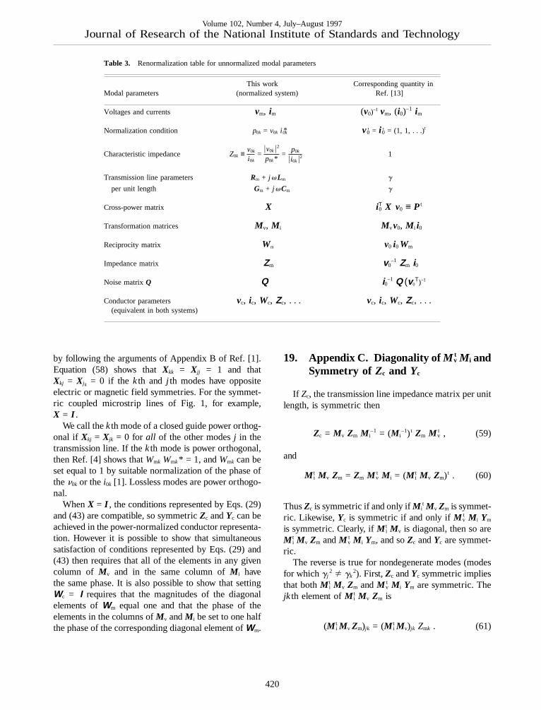
Table 3. Renormalization table for unnormalized modal parameters

This work Corresponding quantity inModal parameters (normalized system) Ref. [13]

Voltages and currents vm, im (v0)–1 vm, (i0)–1 im

Normalization condition p0k = v0k i 0k* v0' = i 0' = (1, 1, . . .)t

Characteristic impedance Z0k ≡ v0k

i0k=

uv0k u2

p0k*=

p0k

ui0k u21

Transmission line parameters Rm + j vLm g

per unit length Gm + j vCm g

Cross-power matrix X i0T X v0 ≡ Pt

Transformation matrices Mv, M i Mvv0, M i i0

Reciprocity matrix Wm v0 i0 Wm

Impedance matrix Zm v0–1 Zm i0

Noise matrixQ Q i0–1 Q (v0

T)–1

Conductor parameters vc, ic, Wc, Zc, . . . vc, ic, Wc, Zc, . . .(equivalent in both systems)

by following the arguments of Appendix B of Ref. [1].Equation (58) shows thatXkk = Xjj = 1 and thatXkj = Xj k = 0 if the kth and j th modes have oppositeelectric or magnetic field symmetries. For the symmet-ric coupled microstrip lines of Fig. 1, for example,X = I .

We call thekth mode of a closed guide power orthog-onal if Xkj = Xjk = 0 for all of the other modesj in thetransmission line. If thekth mode is power orthogonal,then Ref. [4] shows thatWmk Wmk* = 1, andWmk can beset equal to 1 by suitable normalization of the phase ofthen0k or thei0k [1]. Lossless modes are power orthogo-nal.

WhenX = I , the conditions represented by Eqs. (29)and (43) are compatible, so symmetricZc andYc can beachieved in the power-normalized conductor representa-tion. However it is possible to show that simultaneoussatisfaction of conditions represented by Eqs. (29) and(43) then requires that all of the elements in any givencolumn of Mv and in the same column ofM i havethe same phase. It is also possible to show that settingWc = I requires that the magnitudes of the diagonalelements ofWm equal one and that the phase of theelements in the columns ofMv andM i be set to one halfthe phase of the corresponding diagonal element ofWm.

19. Appendix C. Diagonality ofM vt M i and

Symmetry of Zc and Yc

If Zc, the transmission line impedance matrix per unitlength, is symmetric then

Zc = Mv Zm M i–1 = (M i

–1)t Zm M vt , (59)

and

M it Mv Zm = Zm M v

t M i = (M it Mv Zm)t . (60)

ThusZc is symmetric if and only ifM it Mv Zm is symmet-

ric. Likewise,Yc is symmetric if and only ifM vt M i Ym

is symmetric. Clearly, ifM it Mv is diagonal, then so are

M it Mv Zm andM v

t M i Ym, and soZc andYc are symmet-ric.

The reverse is true for nondegenerate modes (modesfor which gj

2 Þ gk2). First,Zc andYc symmetric implies

that bothM it Mv Zm andM v

t M i Ym are symmetric. Thejk th element ofM i

t Mv Zm is

(M it Mv Zm)jk = (M i

t Mv)jk Zmk . (61)

420


Thus M it Mv Zm symmetric implies that (M i

t Mv)jk

Zmk = (M i Mv)kj Zmj . Likewise, M vt M i Ym symmetric

implies (M it Mv)kj Ymk = (M i

t Mv)jk Ymj . Taking theproduct of these two equations and usingZmk Ymk = gk

2

gives (M it Mv)jk (M i

t Mv)kj (gj2 – gk

2) = 0, which leads toeither (M i

t Mv)jk = 0 or (M it Mv)kj = 0. Assume that

(M it Mv)jk = 0. Then, from Eq. (60),

(M it Mv Zm)kj = (M i

t Mv)kj Zmj

= (M it Mv Zm)jk = (M i

t Mv)jk Zmk = 0 , (62)

and so (M it Mv)kj = 0 as well. A similar argument applies

if we assume that it was (M it Mv)kj that was 0. Thus

M it Mv is diagonal.

20. Appendix D. Symmetry of theImpedance Matrices of ReciprocalJunctions and ScalarWc

If Wc is scalar, then Eq. (41) shows that the conductorimpedance matricesZc of all passive junctions con-structed entirely of reciprocal materials embedded in itare symmetric.

If the conductor impedance matrixZc of every pas-sive junction constructed of reciprocal materials embed-ded in it is symmetric, then we can also show thatWc isa scalar. From Eq. (41) we have

Zc = Z ct = Wc Zc (Wc

t)–1 , (63)

which implies that

Zc Wct = Wc Zc . (64)

The ij th element ofZc Wct isO

kZcik Wcjk , while theij th

element ofWc Zc is Ok

Wcik Zckj . Equating these two

elements gives

(Wcjj – Wcii ) Zcij + OkÞj

Wcjk Zcik

– OkÞi

Wcik Zckj = 0, (65)

which must hold true for the conductor impedancematrix of any junction constructed of reciprocal materi-als. For any giveni Þ j , Eq. (65) can only be true for allof theseZc if Wcjj – Wcii and all of the termsWcjk

(k Þ j ) are independently equal to 0, which implies that

Wc is a scalar matrix.Finally, if Wc = aI , wherea is a scalar, then Eq. (42)

shows thatM it Mv = aWm.

If Wc = aI , then Eq. (41) shows that the conductorimpedance matricesZc of all junctions constructedentirely of reciprocal materials connecting the lines toother lines for whichWc = aI will be symmetric. Like-wise, if the conductor impedance matrices of all junc-tions constructed entirely of reciprocal materials con-necting the lines to other lines for whichWc = aI aresymmetric, we must haveWc = aI . This also holds true,of course, whenWc = I in all the lines. This is the mostconvenient normalization sinceWc = I is the naturalchoice in lossless lines.

21. Appendix E. Renormalization Table

We have presented relations between modal andconductor quantities. Here we show how a renormaliza-tion of the conductor voltages and currents thatpreservesM i

T Mv = X affects the other conductorparameters. The second column shows the effect on theelement in the first column after multiplying the voltageeigenvector by the matrixd ≡ diag(dq).

Table 4. Renormalization table for power-normalized conductorparameters

Before normalization After normalization

vc, ic dvc, (d*) –1 ic

Mv, M i d Mv, (d*) –1M i

Zc, Yc d Zc d*, (d*) –1 Yc d–1

Wc, Wc d* Wc d–1, d* Wc d–1

Zc d Zc d*

Mi Q MvT (d*) –1 Mi Q Mv

T d*

22. Appendix F. Form of X and Wm forTwo Modes WhenWc = I

Whenever it is possible to satisfy the power normal-ization condition of Eq. (29) and setWc = I simulta-neously we have bothM i

T Mv = X and M it Mv = Wm.

Thus we can writeX Wm–1 = M i

T Mv Mv–1(M i

t)–1 =M i

T (M it)–1 and so (X Wm

–1)* X Wm–1 = (M i

T (M it)–1)* M i

T

(M it)–1 = I .

Reference [4] shows that the condition (X Wm–1)* X

Wm–1 = I also holds if all the modes in the guide are

accounted for.

421


If, for every modej to which we have assigned avoltage and a current and for every modek for which wehave not, the cross-power integralseetj 3 htk* ? dS =e etk 3 htj * ? zdS = 0, then as a corollary we have(X Wm

–1)* X Wm–1 = I as well.

When (X Wm–1)* X Wm

–1 = I and there are only twomodes, which we will label thec and p modes, then(X Wm

–1)* = (X Wm–1)–1 and we can writeX andWm as

X = F 1Xpc

Xcp

1 G ; Wm = FWmc

00

Wmp

G , (66)

which implies that

3 (Wmc*) –1

Xpc*(Wmc*) –1

Xcp *(Wmp *) –1

(Wmp *) –1 4 =

WmcWmp

1–Xcp Xpc 3 Wmp–1

–XpcWmc–1

–XcpWmp–1

Wmc–1 4 . (67)

Equating the diagonal terms in Eq. (67) implies thatuWmcu2 = uWmp u2 = 1– X cp X pc, which implies that theproductXcp Xpc is real and that we can writeWmc andWmp as Wmc = Ï1–XcpXpc ejuc and Wmp = Ï1–Xcp Xpc

ejup . Equating the upper-right hand off-diagonal termsin Eq. (67) allows us to determine the phase of Xcp interms of uc and up to within a factor of6p , whileequating the lower-left hand off-diagonal terms in Eq.(67) allows us to determine the phase ofXpc. Theseconstraints on the phase ofXcp andXpc, in addition to theconstraint that their product be real, result in the forms

X = 3 1

6j uXpcuej (uc–up )/2

6j uXcp uej (uc–up )/2

1 4 (68)

and

Wm = Ï1–Xcp Xpc Fejuc

00

ejupG (69)

for X andWm, respectively.

Acknowledgments

The authors appreciate the contributions of WolfgangHeinrich and Frank Olyslager to this work.

23. References

[1] R. B. Marks and D. F. Williams, A general waveguide circuittheory, J. Res. Natl. Inst. Stand. Technol.97, 533–561 (1992).

[2] J. R. Brews, Transmission line models for lossy waveguideinterconnections in VLSI, IEEE Trans. Electron Dev.ED-33,1356–1365 (1986).

[3] D. F. Williams and R. B. Marks, Reciprocity Relations inWaveguide Junctions, IEEE Trans. Microwave Theory Tech.41, 11-5–1110 (1993).

[4] D. F. Williams, Thermal noise in lossy waveguides, IEEETrans. Microwave Theory Tech.44 (7), 1067–1073 (1996).

[5] K. D. Marx, Propagation modes, equivalent circuits, and char-acteristic terminations for multiconductor transmission lineswith inhomogeneous dielectrics, IEEE Trans. Microwave The-ory Tech.21 (7), 450–457 (1973).

[6] V. K. Tripathi and J. B. Rettig, A SPICE model for multiplecoupled microstrips and other transmission lines, IEEE Trans.Microwave Theory Tech.33 (12), 1513–1518 (1985).

[7] L. Carin and K. J. Webb, An equivalent circuit model forterminated hybrid-mode multiconductor transmission lines,IEEE Trans. Microwave Theory Tech.37 (7), 1784–1793(1989).

[8] L. Weimer and R. H. Jansen, Reciprocity related definition ofstrip characteristic impedance for multiconductor hybrid-modetransmission lines, Microwave Optical Technol. Lett., 22–25(1988).

[9] L. Carin and K. J. Web, Characteristic impedance of multi-level, multiconductor hybrid mode microstrip, IEEE Trans.Magnetics, 2947–2949 (1989).

[10] R. H. Jansen, Unified user-oriented computation of shielded,covered and open planar microwave and millimeter-wavetransmission-line characteristics, IEE J. Microwaves, Optics,and Acoustics, 14–22 (1979).

[11] V. K. Tripathi and H. Lee, Spectral-domain computation ofcharacteristic impedances and multiport parameters of multiplecoupled microstrip lines, IEEE Trans. Microwave TheoryTech.37 (1), 215–221 (1989).

[12] F. E. Gardiol, Lossy Transmission Lines, Artech House, Inc.,Norwood, MA (1987).

[13] N. Fache´ and D. De Zutter, New high-frequency circuit modelfor coupled lossless and lossy waveguide structures, IEEETrans. Microwave Theory Tech.38 (3), 252–259 (1990).

[14] D. F. Williams and F. Olyslager, Modal cross power in quasi-TEM transmission lines, IEEE Microwave Guided Wave Lett.6 (11), 413–415 (1996).

[15] D. F. Willaims, Calibration in multiconductor transmissionlines, 48th ARFTG Conf. (1996).

[16] T. Dhaene and D. De Zutter, CAD-oriented general circuitdescription of uniform coupled lossy dispersive waveguidestructures, IEEE Trans. Theory Tech.40 (7), 1545–1554(1992).

[17] N. Fache´, F. Olyslager, and D. De Zutter, Electromagnetic andCircuit Modeling of Multiconductor Transmission Lines,Clarendon Press, Oxford (1993).

422


[18] F. Olyslager, D. De Zutter, and A. T. de Hoop, New reciprocalcircuit model for lossy waveguide structures based on the or-thogonality of the eigenmodes, IEEE Trans. Microwave TheoryTech.42 (12), 2261–2269 (1994).

[19] R. E. Collin, Field Theory of Guided Waves, McGraw-Hill,New York (1960).

[20] G. Goubau, On the excitation of surface waves, Proc. I.R.E.,865–868 (1952).

[21] D. F. Williams, Multiconductor transmission line characteriza-tion, submitted to IEEE Trans. Comp. Packag. and Manuf.Tech.20(2), 129–132 (1997).

[22] D. F. Williams, Characterization of embedded multiconductortransmission lines, submitted to 1997 IEEE InternationalMicrowave Theory and Tech. Symp., TH 4D-2.

[23] D. P. Nyquist, D. R. Johnson, S. V. Hsu, Orthogonality andamplitude spectrum of radiation modes along open-boundarywaveguides, J. Opt.. Soc. Am. 49–55 (1981).

[24] T. G. Livernois, On the reciprocity factor for shieldedmicrostrip, Microwave Optical Technol. Lett. (1995).

[25] J. Stoer and R. Bulirsch, Introduction to Numerical Analysis,Springer-Verlag, New York (1980).

[26] H. A. Haus and R. B. Adler, Circuit Theory of Linear NoisyNetworks, John Wiley adn Sons, Inc., New York (1959).

[27] A. van der Zierl, Noise in Measurements, John Wiley & Sons,New York (1976).

[28] W. Heinrich, Full-wave analysis of conductor losses on MMICtransmission lines, IEEE Trans. Microwave Theory Tech.38(10), 1468–1472 (1990).

About the authors: Dylan F. Williams and Roger B.Marks are project leaders in the Electromagnetic FieldsDivision of the Electronics and Electrical EngineeringLaboratory, NIST Boulder. Leonard Hayden joinedNIST as a postdoctoral researcher in 1993. He isnow a Senior Applications Engineer with CascadeMicrotech, Inc. The National Institute of Standards andTechnology is an agency of the Technology Administra-tion, U.S. Department of Commerce.

423

a complete multimode equivalent-circuit theory for ... · a complete multimode equivalent-circuit...

Documents