a comparison study of data assimilation ... -...
TRANSCRIPT

A Comparison Study of Data AssimilationAlgorithms for Ozone Forecasts
CEREA report 2008-6
INRIA-Rocquencourt/ENPC-CEREA, FranceLin Wu, Vivien Mallet, Marc Bocquet, and Bruno Sportisse
lin.wu,[email protected];marc.bocquet,[email protected]
Abstract
The objective of this report is to evaluate the performances of different data assimilationschemes with the aim of designing suitable assimilation algorithms for short-range ozoneforecasts in realistic applications. The underlying atmospheric chemistry-transport modelsare stiff but stable systems with high uncertainties (e.g., over 20% for ozone daily peaks,Hanna et al. [1998]; Mallet and Sportisse [2006b], and much more for other pollutants likeaerosols). Therefore the main difficulty of the ozone data assimilation problem is how toaccount for the strong model uncertainties. In this report, the model uncertainties are ei-ther parameterized with homogeneous error correlations of the model state or estimated byperturbing some sources of the uncertainties, e.g. the model uncertain parameters. Four as-similation methods have been considered, namely optimal interpolation, reduced-rank squareroot Kalman filter, ensemble Kalman filter, and four-dimensional variational assimilation.These assimilation algorithms are compared under the same experimental settings. It isfound that the assimilations significantly improve the one-day ozone forecasts. The compar-ison results reveal the limitations and the potentials of each assimilation algorithm. In ourfour-dimensional variational method, the low dependency of model simulations on initial con-ditions leads to moderate performances. In our sequential methods, the optimal interpolationalgorithm has the best performance during assimilation periods. Our ensemble Kalman filteralgorithm perturbs the uncertain parameters to approximate model uncertainties and hasbetter forecasts than the optimal interpolation algorithm during prediction periods. Thiscould partially be explained by the low dependency on the uncertainties in initial conditions.The sensitivity analysis on the algorithmic parameters is also conducted for the design ofsuitable assimilation algorithms for ozone forecasts.

1 Introduction
A typical Eulerian atmospheric chemistry-transport model (CTM) computes the concentrationsc of a set of chemical species by solving the system of advection-diffusion-reaction equations:
∂ci
∂t= −div(Vci) + div(ρD∇ci
ρ) + χi(c, t) + Ei , ∀i, (1)
where ci is the concentration of the i-th species, V is the wind velocity, ρ is the air density, Dis the turbulent diffusion matrix, χi(c, t) stands for the species production and loss due to thechemical reactions, and Ei stands for the elevated emissions. At ground the boundary conditionis given by
−ρD∇ci
ρ· n = Si − vdep
i ci , (2)
where n is the upward unitary vector, Si stands for the surface emissions and vdepi is the dry
deposition velocity.
In the numerical model (the CTM), the dimension of the discretized system is usually 106–107. The model computes ozone hourly concentrations over Europe (for instance) given theinitial conditions and the input data (also designated herein as parameters).
Data assimilation can be considered as the determination of the initial conditions or ofmodel uncertain parameters by coupling the heterogeneous available information, e.g. modelsimulations, observations, and statistics for errors. Data assimilation methods are roughly cat-alogued into variational and sequential ones [Le Dimet and Talagrand, 1986; Evensen, 1994].The objective of the former can be defined as state estimation by minimizing the quadratic dis-crepancy between model simulation and a block of observations, usually combined with a prioribackground knowledge. This can be formalized and solved efficiently with the optimal controltheory. The sequential methods make use of observations as soon as they are available. Sincethis is a filtering process, filter theory (linear or nonlinear) applies.
Both methods have found their applications for CTMs. The pioneering work dates back toFisher and Lary [1995]. On the variational side, Elbern and Schmidt [2001] use a comprehensivemodel rather than an academical model in order to assimilate real observations with assessmentof ozone forecast. Chai et al. [2007] follow with assimilation of new types of observations, andseveral practical issues, e.g. background error modeling, are investigated with details. Very fewwork deals with the assimilation of initial conditions jointly with uncertain parameters [Elbernet al., 2007]. By contrast, Segers [2002] conducts in-depth studies on the applications of efficientfiltering methods, in which emissions, photolysis rates and deposition are considered to be un-certain. The model state as well as uncertain parameters are estimated. Constantinescu et al.[2007b] report the filtering results obtained with perturbations on emissions and on boundaryconditions, and with distance constraints on the spatial correlations.
All these efforts are part of the recent diffusion of data assimilation expertise from numer-ical weather prediction (NWP) to air quality community. For a review see Carmichael et al.[2008]. The CTMs are stiff but stable systems; the perturbations on initial conditions tend to besmoothed out rather than amplified. Therefore the conclusions from meteorological experiences[Lorenc, 2003; Kalnay et al., 2007] cannot be applied directly.
The objective of this report is to evaluate different assimilation algorithms for ozone forecastsin the same experimental settings. Hopefully this could serve as a base point for the design ofassimilation algorithms suitable for ozone forecasts in realistic applications. Four algorithms,namely optimal interpolation (OI), ensemble Kalman filter (EnKF), reduced-rank square rootKalman filter (RRSQRT) and four-dimensional variational assimilation (4DVar) were imple-mented.
2

We note that this comparison study has its limitations in that: i) Only model state is adjustedand uncertain model parameters remain unchanged. ii) The treatment of uncertainties aredifferent. OI parameterizes aggregate uncertainties using the homogeneous Balgovind correlationfunction. In 4DVar the uncertainties are taken into account, in a way similar to OI (Balgovindcorrelation), but only at the initial date of the assimilation period. The underlying model isassumed to be perfect, that is, we consider a strongly constrained 4DVar. By contrast, EnKFand RRSQRT represent model uncertainties with ensemble generated by Monte Carlo samplingsof uncertain parameters. The reasons for the first limitation are that (1) the adjoint model withrespect to model parameters is not available, and (2) correlations between the model state andparameters are unknown. Clearly this should be a research task in near future. The secondlimitation stems from the unsettled formulation of model error. A novelty of our EnKF andRRSQRT implementation is the perturbation method, originally employed in uncertainty studiesfor air quality models [Hanna et al., 2001].
The report is organized as follows. Section 2 documents the assimilation algorithms andtheir implementations. The experiment setup concerning the model and observations is detailedin Section 3. We report the comparison results in Section 4. Therein sensitivity studies withrespect to the assimilation algorithm settings are also conducted. Conclusions and discussionscan be found in Section 5.
2 Assimilation Algorithms
We rewrite the CTM dynamical differential equation in discrete form from time tk−1 to tk,
xt(tk) = Mk−1
(xt(tk−1)
)+ ǫf (tk−1) , (3)
where xt denotes the true state vector of dimension n, Mk−1 corresponds to the (nonlinear)dynamical operator from k − 1 to k, and ǫf is the model error vector assumed to have a normaldistribution with zero mean and covariance matrix Q. In this study, the state is chosen to bethe vector of concentrations for the concerned species. For simplicity we drop tk to subindex k,e.g. xt
k for xt(tk) and Qk−1 for Q(tk−1). At each time tk, one observes,
yk = Hk
(xt
k
)+ ǫo
k , (4)
where ǫok is the observation error vector assumed to have a normal distribution with zero mean
and covariance matrix R, and Hk is the (possibly nonlinear) operator that maps the state to theobservation space at time tk. The vector yk is of size p, and usually p ≪ n. The error vectorsǫfk−1 and ǫo
k are supposed to be independent.
Let xb be the a priori state estimation (background) with error ǫb = xb − xt of zero meanand covariance matrix B, and let xa be the posterior state estimation (analysis) with errorǫa = xa − xt of covariance matrix A. The data assimilation problem is to determine theoptimal analysis xa and its statistics A given background xb, observation y, and the statisticalinformation in error covariance items R and B.
2.1 Optimal Interpolation
Optimal interpolation [Daley, 1991] searches for an optimal linear combination between back-ground and innovation by minimizing the state-estimation variance. The innovation d is the dif-ference between the observation vector and the state vector, i.e. d = y−H(xb). Under linearityassumption of the observation operator close to the background, i.e. H(x)−H(xb) = H(x−xb)
3

where H is the linearized operator, the estimation formulae are given according to best linearunbiased estimator theory as follows,
xa = xb + K(y − H(xb)) , (5)
K = BHT (HBHT + R)−1 . (6)
In practice, setting the background error covariance remains problematic. In this study B iseither diagonal or in Balgovind form. In the latter case, the error covariance between two pointsis given by
f(d) =
(
1 +d
L
)
e−d
L v , (7)
where L is a characteristic length, d is the distance between the two points, and v is the a priorivariance [Balgovind et al., 1983].
2.2 Ensemble Kalman Filter
Ensemble Kalman filter [Evensen, 1994, 2003] differs from optimal interpolation in that the errorcovariance matrix is time-dependent. The assimilation process follows the cycling of two stepsof forecast and analysis. At forecast step, the model is applied to the r−member ensemble
xa,(i)k−1 , i = 1, . . . , r, and produces the forecast xf,(i)
k , i = 1, . . . , r. The forecast error covari-
ance matrix Pf can be approximated by the ensemble statistics. Whenever observations are
available, the cycling enters into analysis step, and each ensemble member xf,(i)k is updated to
xa,(i)k according to the OI formula (5-6), with background error covariance matrix B replaced
by forecast error covariance matrix Pf . Although not necessary in the algorithm, the analysiserror covariance matrix Pa can then be approximated with the analyzed-ensemble statistics.
We summarize the algorithm as follows,
• Initialization: given the probability density function (PDF) of the initial concentrations,an ensemble of initial conditions is generated. In our experiments, except for the cyclingcontext in Section 4.4 where initial ensemble members are ensemble forecasts from theprevious cycle, we skip this step: all members in the ensemble start with the same initialcondition. The first integration steps are therefore a spin-up period during which theensemble spread is essentially increasing as a result of the perturbations on uncertainparameters.
• Forecast step:
xf,(i)k = Mk−1
(
xa,(i)k−1
)
+ ǫf,(i)k−1 , (8)
Pfk =
1
r − 1
r∑
i=1
(
xf,(i)k − xf
k
) (
xf,(i)k − xf
k
)T
, (9)
where xfk is the mean of the forecast ensemble: xf
k = 1r
∑ri=1 x
f,(i)k .
• Analysis formula:
xa,(i)k = x
f,(i)k + Kk
(
y(i)k − Hk
(
xf,(i)k
))
, (10)
Pak =
1
r − 1
r∑
i=1
(
xa,(i)k − xa
k
) (
xa,(i)k − xa
k
)T
, (11)
4

where xak is the mean of analysis ensemble xa,(i)
k , i = 1, .., r, y(i)k is the observation vector,
and the Kalman gain is approximated by
Kk = PfkH
Tk
(
HkPfkH
Tk + Rk
)−1. (12)
The ensemble initialization and the determination of the model error ǫf,(i)k−1 are entangled
problems. In our implementation, we take identical initial samples, and the model error isapproximated by perturbing model input data and model parameters:
ǫf,(i)k−1 ≃ Mk−1
(
xa,(i)k−1 ,w(i)d
)
− Mk−1
(
xa,(i)k−1 ,d
)
, (13)
where d is the vector of parameters to be perturbed, and for i−th sample, w(i) is the diago-
nal matrix whose diagonal elements are perturbation coefficients (see Section 2.5). Let ef,(i)k
be xf,(i)k − xf
k , one (approximate) direction of the forecast error, and let Efk be the matrix
[ef,(1)k e
f,(2)k . . . e
f,(r)k ]. By formula (9), we have
Pfk =
1
r − 1EET . (14)
In this way, the error covariance matrix is approximated by ensemble statistics.
In the original EnKF algorithm, the observation vector y(i)k is perturbed for consistent analy-
sis statistics [Burgers et al., 1998]. In this report, we present only the assimilation results withoutobservation perturbations, since the variances of observation errors are in general much smallerthan those of model errors. However, in our implementation, the observation perturbation is anoption, and preliminary tests showed that, at least for the reference setting in Section 3, thereare improvements in forecast performance with this option on.
2.3 Reduced-Rank Square Root Kalman Filter
Reduced-rank square root Kalman filter [Heemink et al., 2001] uses a low-rank representationLLT of error covariances matrix P. L = [l1, . . . , lq] is the mode matrix whose columns (modes)are the dominant directions of the forecast error. The evolution of a mode can be approximatedby the differences of the forecasts based on the mean (analyzed) state and its perturbation bythis mode, that is,
lf,(i)k = Mk−1
(
xak−1 + l
a,(i)k−1
)
− Mk−1
(xa
k−1
), (15)
where xak−1 is given by
xak−1 = xf
k−1 + Kk−1
(
yk−1 − Hk−1
(
xfk−1
))
. (16)
The forecast xfk−1 is calculated from previous analyzed state by
xfk−1 = Mk−2
(xa
k−2
). (17)
Assuming that at time tk−1 the error covariance Pak−1 has the square root form La
k−1La,Tk−1,
the propagation of Pak−1 is tractable. The forecast error covariance matrix at time tk is calculated
by
Pfk = Mk−1P
ak−1Mk−1
T + Qk−1
=
[
Mk−1Lak−1 Q
1
2
k−1
] [
Mk−1Lak−1 Q
1
2
k−1
]T
,(18)
5

where Mk−1 is the tangent linear model, that is the Jacobian matrix of Mk−1, Q1
2
k−1 is the
square root of model error covariance matrix. Considering square root form LfkL
f,Tk for Pf
k , wehave the forecast formula for mode matrix Lf :
Lfk = [Mk−1L
ak−1 Q
1
2
k−1], Lfk = Πf
kLfk , (19)
where Πfk projects Lf
k onto the q leading eigenvectors of LfkL
f,Tk using the singular value decom-
position. Recall that analysis error covariance matrix Pa can be calculated by (I−KH)Pf (I−KH)T +KRKT for arbitrary gain K, then rewriting it in square root form we obtain the analysisformula for mode matrix La:
Lak = [(I − KkHk)L
fk KkR
1
2
k ], Lak = Πa
kLak , (20)
where Πak projects La
k onto the q leading eigenvectors of LakL
a,Tk .
We do not use the tangent linear model, but employ (15) to simulate Mk−1Lak−1 at forecast
step. The columns of Q1
2
k−1 are obtained in the same manner as the model error formula (13)in EnKF. The above treatments make the RRSQRT implementation similar to our variant ofEnKF. The difference is that RRSQRT employs square root formulae. In addition, the errorcovariance is approximated in dominant eigenvectors in RRSQRT whereas EnKF bears no suchprocess.
2.4 Four-Dimensional Variational Algorithm
Four-Dimensional Variational Algorithm [Le Dimet and Talagrand, 1986] finds the optimal initialcondition x∗ by minimizing a cost function:
J(x) =1
2(x − xb)TB−1(x − xb)
︸ ︷︷ ︸
Jb
+
1
2
N∑
k=0
(yk − Hk(xk))T R−1
k (yk − Hk(xk))
︸ ︷︷ ︸
Jo
(21)
under the constraint xk = M0→k(x) = Mk−1 (Mk−2 (. . .M1 (M0(x)) . . .)). The assimilationperiod is from t0 to tN . The gradient for Jo is calculated by the backward integration of theadjoint model [Bouttier and Courtier, 1999]:
• xN = 0 ,
• For k = N, . . . , 1, calculates xk−1 = MTk−1
(xk − HT
k dk
), where dk = R−1
k (yk − Hk(xk)) ,
• x0 := x0 − HT0 (d0) gives the gradient of Jo with respect to x.
Assimilations are performed by model integrations starting from the optimal initial conditionx∗. Further integrations from time step N based on the analyzed model state provide the predic-tions. The inverse of B is calculated online or, for high dimensional model configurations, B−1
can also be approximated using SVD truncations and saved on disk for later computations. Theadjoint operator MT
k−1 is obtained using the automatic differentiation software O∂yssee [Faureand Papegay, 1998]. The forward model simulations are saved for the backward integrations ofthe adjoint model. No checkpointing technique is employed in our implementation.
6

2.5 Uncertainties and Model Error
The corrections of the analysis scheme lie in the subspace spanned by covariance matrix offorecast or background errors, i.e., the space induced by the columns of the square root of thematrix B [Kalnay, 2003]. Unrealistic error structure produces spurious corrections, and probablyresults in unbalanced physical model state. Therefore the design of the error structure is of greatimportance.
There are mainly three approaches for error modeling: i) modeling uncertain sources andthen perturbing them in the model [Segers, 2002; Constantinescu et al., 2007a]; ii) using thestatistics of model states, e.g. NMC method [Chai et al., 2007] and ensemble methods; iii) usingparameterizations, e.g. Balgovind correlations for background error covariance [Hoelzemannet al., 2001; Elbern et al., 2007]. Each of the three should be flow-dependent, that is, adaptingto the “error of the day”. The spatial and temporal heterogeneities of the chemistry-transportproblem make the last two approaches difficult issues.
The numerical models are usually assumed unbiased. In our case, we assume that the modeluncertainties only result from the misspecification of model parameters. In our EnKF andRRSQRT implementation, the ensemble is generated by the model integrations with perturbedparameters. The uncertainties and the distributions are introduced for model parameters thatare mainly bidimensional or tridimensional fields under space coordinates. These parametersare modeled as random vectors. In practice, for a field p (a random vector) whose median valueis p, a perturbation is applied to the whole field so that every component pi
k has the prescribeddistribution. For instance, for a lognormal distribution, one writes
pik = pi
k ×√
αγ
, ∀k, i (22)
where γ is sampled according to a standard normal distribution. The quantity γ is independentof the time index k and of the space index i, so that the perturbations increase the ensemblespread. The same sample of γ is used to perturb all values of the field p. The quantity
√α
γ
is the perturbation coefficient for the corresponding parameter in matrix w(i) in formula (13).For normal distributions, perturbations bigger than certain given quantity (by default two timesof the standard deviation) are discarded so that no unrealistic parameters are produced, forinstance, the negative emissions.
A delicate point is having temporal and spatial correlations between the different values ofthe field. With the perturbation applied in (22), the correlation between two field values ln pi
k
and ln pjl is equal to 1. But the uncertainty sources at these two points are not the same; hence
the perturbation should be different. A fine modeling of the uncertainty should lead to haveγ depending on time and position (producing γi
k). Such a fine description of uncertainties ismostly beyond available knowledge.
Examples for continental air quality simulations extracted from Hanna et al. [2001] are shownin Table 1. For many fields (associated with α = 2), a confidence interval that includes 95% ofthe probability density integral is [m2 , 2m] if m is the mean of the field. Uncertainty levels mustbe adjusted to the simulation scale (domain size and temporal discretization). In particular,uncertainties decrease as data is averaged over a larger domain or over a longer period of time.
3 Experiment Setup
3.1 Model and Input Data
The ozone forecasts and the assimilation experiments are performed in the framework of theair quality modeling system Polyphemus [Mallet et al., 2007] whose version 1.2 includes all
7

Field Distribution Uncertainty
Top ozone boundary conditions log-normal α = 1.5Top NOx boundary conditions log-normal α = 3Lateral ozone boundary conditions log-normal α = 1.5Lateral NOx boundary conditions log-normal α = 3Major NOx point emissions log-normal α = 1.5Wind velocity log-normal α = 1.5Wind direction normal ±40
Temperature normal ±3 KVertical diffusion (night) log-normal α = 3Precipitations log-normal α = 2Cloud liquid water content log-normal α = 2Biogenic emissions log-normal α = 2Photolysis constants log-normal α = 2
Table 1: Uncertainties associated with several input fields of a chemistry-transport model atcontinental scale. The uncertainty of a parameter p is measured with a confidence interval thatincludes 95% of the probability density integral. For a log-normal distribution, this interval isdefined by a factor α so that p is in the interval [ p
α, αp] with a probability of 95% (p is the
median value of p). All estimates were derived from Hanna et al. [2001].
algorithms in use in this report and is freely available at http://cerea.enpc.fr/polyphemus/.For this study, the Polyphemus model in use is Polair3D [Boutahar et al., 2004] for which
an adjoint version is available (for gas-phase chemistry). The configuration of the model maybe roughly described as follows:
1. raw meteorological data: ECMWF†1 fields (resolution of 0.36 × 0.36, 60 vertical levels,time step of 3 hours, 12 hours forecast-cycles starting from analyzed fields);
2. land use coverage: GLCF†2 land cover map (14 categories, 1 km Lambert);
3. chemical mechanism: RACM [Stockwell et al., 1997];
4. emissions: the EMEP†3 inventory, converted according to Middleton et al. [1990];
5. biogenic emissions: computed as proposed in Simpson et al. [1999];
6. deposition velocities: the revised parameterization from Zhang et al. [2003];
7. vertical diffusion: the Troen and Mahrt parameterization [Troen and Mahrt, 1986] (in theunstable boundary layer) and the Louis parameterization [Louis, 1979] (elsewhere);
8. boundary conditions: typical concentrations from the global chemistry-transport modelMozart 2 [Horowitz et al., 2003];
9. numerical schemes: a first-order operator splitting, the sequence being advection–diffusion–chemistry; a direct space-time third-order advection scheme with a Koren flux-limiter; asecond-order order Rosenbrock method for diffusion and chemistry [Verwer et al., 2002].
†1European Centre for Medium-Range Weather Forecasts†2Global Land Cover Facility†3Co-operative Programme for Monitoring and Evaluation of the Long-range Transmission of Air Pollutants in
Europe
8

The model domain essentially covers Western Europe ([35.0N, 10.5W] × [57.5N, 22.5E]).Two meshes are considered. The reference mesh has a 0.5 horizontal resolution, and the altitudeof the tops of the vertical layers are 50 m, 600 m, 1200 m, 2000 m and 3000 m. The top layeris high enough to enclose the planetary boundary layer. A time step of 600 s is used. Thecoarse mesh has a 2 horizontal resolution and it includes three levels whose top heights are50 m, 600 m and 1200 m. The time step is set to 1800 s. Both models have 72 chemical species(with RACM) mechanism. Hence the dimension of the state vector is about 1.1 × 10⁶ for thefull-resolution model and 3.8 × 10⁴ for the coarse-resolution model.
An analysis of the simulations with the coarse mesh demonstrates that the main physicalphenomena (at least for ozone) are reasonably reproduced in the context. The model retainsgood predictive capabilities (see the comparisons with observations in Section 4). The coarsecase is used to perform intensive tests. For instance, in the Kalman algorithms that we use,the results depend on random numbers. Thus, they can only be assessed from a large numberof trials, which is not tractable with the full resolution model. Nevertheless the full resolutionstudy will be carried out later to verify some key findings in the coarse case.
The horizontal domain and its coarse discretization are shown in Figure 1.
-10 -5 0 5 10 15 20
Longitude (degrees)
35
40
45
50
55
Lati
tud
e (
deg
rees)
Figure 1: Horizontal coarse discretization of model domain. The squares show the locations ofEMEP monitoring stations, and the disc shows the location of the monitoring station Montandon(east of France).
3.2 Observations
The observations to be assimilated are ozone hourly concentrations. These observations areprovided by the EMEP†4 network (Figure 1). The network is made of 151 ground stations amongwhich 80–90 stations are actually available during the assimilation periods. They deliver pointmeasurements integrated over one hour, but we assume that the observations are instantaneous– as it better fits the algorithms implementation.
The EMEP network includes only regional stations, which ensures a proper comparisonbetween the continental-model outputs and the observations. The model outputs are linearlyinterpolated (on the horizontal, not on the vertical) at the station locations – the observationoperator Hk is therefore linear and its adjoint is easily derived.
†4Co-operative Programme for Monitoring and Evaluation of the Long-range Transmission of Air Pollutants inEurope
9

It is assumed that the error covariance matrix for ground ozone observations is diagonal,which is reasonable as the measurements from two stations are performed by distinct instru-ments. The standard deviation of the observation error is set to 10 µg m−3 [Flemming et al.,2003]. Note that the mean of ozone observations is about 70 µg m−3.
3.3 Reference Settings of the Assimilation Algorithms
In this section, we list our default settings of the assimilation algorithms. Sensitivity studies willbe performed by alternating algorithm settings in later sections. The experiments consist of twosteps: assimilation and prediction. During the assimilation period, say [t0, tN ], the observationsare assimilated, and during the subsequent prediction period, say [tN+1, tT ], the ozone forecastsare the model simulations starting from the analyzed model state at tN . In the reference settingthe assimilation period is one day from 1st July 2001 at 01:00 UT to 2nd July at 00:00 UT. Theprediction period is one day from 2nd July 2001 at 01:00 UT to 3rd July at 00:00 UT.
The model nonlinearity imposes an upper limit on the time length of the assimilation period(hereafter referred to as assimilation window). Previous perturbations out of this upper limitare ignored. In fact, driven by the winds, the pollutants may be transported out of the modelingdomain after a few days. There is also a lower limit during which the impact of the assimilatedobservations propagates over the whole model domain. In meteorology, the assimilation timeinterval is about 6 hours extendable to 12 hours. In this study, the assimilation window is setto one day.
In the reference setting the state vector includes only ozone concentrations of the first twolevels in the model domain. The correlations are supposed to expand gradually, through modelsimulations, to the complete model domain and to the species other than ozone.
In the Balgovind parameterization of the background error covariance matrix, the standardderivation
√v is set to 20 µg m−3 (derived from usual rmse for ozone forecast and from Mallet
and Sportisse [2006b]), and the characteristic length is set horizontally to 3 (Lh), verticallyto 200 m (Lv). The details about the uncertain parameters to be perturbed for EnKF andRRSQRT will be given in Section 4.2.2.
The EnKF ensemble number r is chosen to be 30. For a comparable computational cost,in RRSQRT, the number of columns q of the mode matrix is set to 20, the number of columnsof the square root Q
1
2 is set to 10, and the number of columns of the square root R1
2 is set to10. In 4DVar, we employ the L-BFGS optimization solver [Byrd et al., 1995]. In this study, thecomputational cost of the adjoint model is about 5–7 times larger than that of the forward model,consequently the number of iterations is set to 6 so that the 4DVar cost may be comparable. Notethat less iterations make 4DVar sub-optimal. However, we checked the evolution of the 4DVarcost function against iteration numbers, and found no considerable decrease in cost functionvalues after 6 iterations (results omitted here).
4 Results
4.1 Coarse-Resolution Case
Let s be the vector of model outputs along space and time and o the vector of correspondingobservations, the performance of ozone forecasts or assimilations can be assessed by the rootmean square error (rmse) calculated as
√√√√
1
n
n∑
i=1
(si − oi)2 (23)
10

where n is the total number of available observations. The rmse over a certain period withrespect to all available observations is called score. In this paer, the rmse will always be givenin µg m−3 · Hereafter this unit will be omitted for convenience.
The four assimilation algorithms provide better forecast scores compared to the referencesimulations (model solutions without assimilation of observations), of course during the assimila-tion period (hourly forecasts for sequential assimilations), but also in the subsequent predictionsteps (see Figure 2). OI has the best overall score, probably because the Balgovind parameter-ization of model error applies well to this coarse test case. From Figure 3, 4DVar has betterscores during the early assimilation period but performs worse during the prediction period.The main reason may be that the underlying 4DVar is strongly constrained, that is, there is nomodel error term in its cost function. Only initial concentrations are controlled. The correctionon the initial concentrations tends to be forgotten by the stable chemistry-transport system.EnKF provides the best performances during the late prediction period. It might benefit fromits manner of perturbations on uncertain parameters. In OI, it can be considered that themodel uncertainties are parameterized by the correlation in model states (which will be theinitial conditions for following forecasts). The impact of model uncertainties in these initialconditions gradually fades out, when the model uncertainties in uncertain parameters (listedin Section 4.2.2) play an increasingly important role during the prediction period. RRSQRTshows poor performance against EnKF. This is probably due to the projection of mode matricesonto the leading eigenvectors of error covariance matrices. For a comparison of the assimilationperformance between EnKF and RRSQRT, we refer to Hanea et al. [2004]. Note that in thatpaper, colored gaussian noises were added on several uncertain parameters, which is differentfrom our perturbation method. The ozone forecasts at EMEP stations are plotted in Figure 4and Figure 5. Most forecasts are between the reference simulations and the observations. Allforecasts during the predictions period approach to the reference in the end. This shows againthe rather low dependency of the short-range predictions on the initial conditions.
Caution has to be paid to the conclusions since the assimilation results can still be improvedby optimal tuning of algorithm parameters.
Reference OI EnKF 4DVar RRSQRT14
16
18
20
22
24
26
28
30
32
Score
s
day #1
day #2
Figure 2: Scores of ozone concentrations during the assimilation period (day #1) and the pre-diction period (day #2).
4.2 Sensitivity Studies for the Coarse Case
The first set of tests is carried out in the coarse case. Modifications of configurations on eachcomponent of the data assimilation systems, i.e. model, observation and algorithm, may influ-
11

0 10 20 30 40
Hours
10
15
20
25
30
35
40
RM
SE
ReferenceOIEnKFRRSQRT4DVar
Figure 3: Time evolution of the rmse for the ozone forecasts. The score over two days is 27.76 forreference, 19.90 for OI, 23.11 for EnKF, 21.98 for 4DVar, and 24.63 for RRSQRT. The verticallines delimits the assimilation period from the prediction period.
0 10 20 30 40 50
Hours
40
50
60
70
80
90
100
110
120
3−
m·
gµ
ReferenceOIEnKFRRSQRT4DVarObs.
Figure 4: Time evolution of average ozone forecasts over all available stations. The error barshows the average spread of the EnKF forecast ensemble calculated over these stations.
0 10 20 30 40
Observation numbers
20
40
60
80
100
120
140
160
3−
m·
gµ
ReferenceOIEnKFRRSQRT4DVarObs.
Figure 5: Time evolution of ozone forecasts against available observations over two days atEMEP station Montandon.
12

ence the assimilation performance. The main difficulty to interpret the results is that the errorcovariance structures B and Pf are unsettled subjects.
As for model component, we examine different state vectors to be controlled, alternativemodel physical parameterizations, Balgovind parameterization of background error covariance,and various perturbation settings for model error approximations. As for observation compo-nent, the error variance ratio between observations and background concentrations is examined.Different observation networks are tested. As for algorithm component, we evaluate the impactof the assimilation time length and EnKF ensemble issues, i.e. ensemble size and randomness.Hopefully some clues can be drawn for error modeling from the results of this sensitivity study.If not mentioned, only one factor is changed in each sensitivity study, and all other algorithmsettings remain the same as those in Section 3.3.
4.2.1 Ensemble Randomness and Size
An important parameter for EnKF is its ensemble size. The directions of model error areapproximated by the samples deviations from the ensemble mean. Recall formula (13), thesedirections are related to the outcomes of the parameters perturbations. A key question for thisapproach is how fast the assimilation results converge as the ensemble size increases. The spreadof the model error space is determined not only by the ensemble size but also by the definitionof the parameters set to be perturbed. The latter is addressed in the following section.
In this section, we conduct EnKF assimilations with ensembles of sizes 5, 10, 20, 30, 50, 70,90 and 120. For each ensemble, the randomness of Monte Carlo sampling is accounted for byemploying 10 different seeds for the random number generation. This means that 10 ensemblesare generated for each ensemble size.
The forecast scores over both the assimilation period and prediction period are shown in Fig-ure 6. Both converge as the ensemble size increases. The influence of the ensemble randomnessdecreases with ensemble size (see the errorbars). The augmentation of sample numbers improvesforecast scores, but the improvements are modest probably due to the fast convergence of theprocedure.
5 10 20 30 50 70 90 120
Ensemble size
21
22
23
24
25
26
Fore
cast
score
s
day #1
day #2
Figure 6: Forecast scores of EnKF against the ensemble size. The score for reference simulationwithout assimilation is 29.55 over day #1, and 25.87 over day #2. The curve shows mean scoresand the errorbar shows the standard derivations over 10 random seed numbers.
The computational cost is proportional to the number of samples in the ensemble. Thebalance between computational cost and assimilation performance helps the specification of the
13

ensemble size. For realistic model grids, there is usually a constraint of 30 ∼ 100 ensemblesamples due to computational considerations.
4.2.2 Uncertain Parameters Setting
Different parameters sets and perturbation magnitudes are listed in Table 2. The uncertainparameters are input data to the model. The perturbation magnitudes are kept reasonable(within the confidence interval at the 95% level), so that no instabilities may be produced dueto the physically unrealistic parameter values. Notice that these parameters are only perturbedin Polair3D which chiefly carries out the numerical time integration. For instance, the per-turbation of the temperature has no impact on the deposition velocities which are computedin preprocessing steps. The forecast scores with respect to uncertain parameters settings areshown in Figure 7. The results in the prediction period are slightly sensitive to the differentuncertain parameters sets, which is consistent with the finding in Mallet and Sportisse [2006b]that the turbulent closure introduces the highest uncertainty. The results are more sensitive tothe uncertain parameters sets than to the perturbation magnitudes. This probably indicatesthat the dimensionality of the bases of the perturbation parameter space are more importantthan the lengths of these bases for assimilations.
The perturbation magnitudes are spatiotemporally homogeneous in this study:√
αγ
in equa-tion (22) does not depend on spatial coordinates, and temporal correlations are not taken intoaccount. However this hypothesis is not necessarily true. Refined perturbations might improvethe forecast performances. Furthermore, additional uncertain parameters may be included fora larger model error spread.
Parameter name α0 α1 α2
Ω0
Boundary condition 3. 3. 3.Deposition velocity 1.5 2. 3.Photolysis rate 1.3 1.5 2.Surface emission 1.5 2. 3.Attenuation 1.3 1.5 2.Vertical diff. coef. 1.3 1.5 2.
Ω′
Cloud height 1.3 1.5 2.Vertical wind 1.3 1.5 2.Meridional wind 1.3 1.5 2.Zonal wind 1.3 1.5 2.Specific humidity 1.3 1.5 2.
Ω′′
Pressure 1.3 1.5 2.Air density 1.3 1.5 2.Merid. diff. coef. 1.3 1.5 2.Zonal diff. coef. 1.3 1.5 2.Temperature 0.005 0.01 0.015
Table 2: Definition of uncertain parameters. Let Ω0 be the set of parameter names for thereference setting in Section 3.3. Let Ω′ and Ω′′ be the two sets of additional parameter names.We denote Ω1 as Ω, Ω′, and Ω2 as Ω, Ω′, Ω′′. The perturbation magnitude is characterizedby α defined as in equation (22). The reference magnitudes are listed in α0 column. In α1
and α2 columns, enlarged magnitudes are defined. Note that the distribution of temperature issupposed to be normal, and its magnitude should be interpreted as relative standard derivation.
14

0 0α;Ω 1 0α;Ω 2 0α;Ω 0 1α;Ω 0 2α;Ω 1 1α;Ω
Uncertain parameters set
16
18
20
22
24
26
Fore
cast
score
s
ensemble 30ensemble 90
Figure 7: Forecast scores for EnKF against different uncertain parameter definitions. Theparameter sets and perturbation magnitudes are defined in Table 2; Ω0; α0 is the referencesetting. The EnKF sample number is chosen to be 30 (white columns) and 90 (dark columns)respectively. The two columns of scores for each case show the forecast scores during theassimilation and prediction periods. The bar values are mean scores, and the errorbar showsthe standard derivations over 10 random seed numbers.
4.2.3 Assimilation Window
This determination of an optimal assimilation window is essentially linked with model nonlin-earity, but should be treated separately according to sequential or variational context. In thevariational case, the model nonlinearity makes the cost function nonconvex, and thus the op-timization may suffer from the presence of local minima. Clearly there are constraints on theassimilation window, and for better performance the assimilation window has to be short [Pireset al., 1996]. In the sequential case, the observations are assimilated spontaneously. There arecorrections on the state vector until the end of the assimilation window, which is an advantagefor the subsequent prediction steps. Elegant analysis demands in-depth investigations on howthe information (from observation) propagates among state components.
We perform brute-force tests. In the sequential case, the prediction period is fixed from 8th
July 2001 at 01:00 UT to 9th July at 00:00 UT, whereas the assimilation window varies from 1day to 7 days and always ends at 00:00 UT 8th July. The algorithm settings are the same asthose for the reference case. For EnKF, the random seed is fixed with an ensemble size set to 30and 90. The forecast scores over the prediction period are compared in Figure 8. We observe aconsiderable improvement in forecast scores with a window of 2 days against that with one daywindow. The first day of assimilation could be interpreted as an ensemble initialization, since theinitial conditions of all members are identical in our implementation. We performed ensembleforecasts starting from identical samples and checked the ensemble spread (results not presentedhere), and we found out that the spread reached its maximum within 10 hours. This explainswhy a one-day assimilation with EnKF may be unsatisfactory. EnKF with longer assimilationwindows (more than 2 days) outperforms OI in this experiment. Larger assimilation windows(more than 5 days) tend to be unnecessary long since the corrections are rapidly forgotten bythe model.
In the variational context, we perform an experiment with the setting as that of the sequentialcase. The assimilation windows varies from 1 to 4 days, followed by one day of prediction. Thestart date of the prediction period is fixed at 01:00 UT 8th July 2001. The forecast scores areshown in Figure 9. The performances over prediction period decrease with longer assimilation
15

1 2 3 4 5 6 7
Assimilation days
20
21
22
23
24
25
26
Fore
cast
score
s
EnKF: 30 samples
EnKF: 90 samplesOI
Figure 8: Forecast scores of OI and EnKF (with 30 and 90 members) against the number ofassimilation days.
periods and approach the score of reference simulation without assimilation. These resultsclearly indicate the limitation of strongly constrained 4DVar in which only initial conditions arecontrolled. Model error has to be taken into account to form the weakly constrained 4DVar forbetter forecast performance.
1 2 3 4
Assimilation days
20
22
24
26
28
30
32
34
36
Fore
cast
score
s
Figure 9: Forecast scores against the number of assimilation days for the two experiments using4DVar.
4.2.4 Physical Parameterization
In order to assess the robustness of the assimilation, we apply EnKF to modified models whichdiffer in their physical parameterizations. Several alternatives to the reference parameterizationsare listed in Table 3, and the corresponding assimilation results are shown in Figure 10. Theassimilations are performed using reference EnKF algorithm with 30 samples. The forecastscores are highly sensitive to the chemical mechanism, as in the uncertainty investigations ofMallet and Sportisse [2006b].
16

Parameterization Reference Alternative
Deposition velocities Zhang Wesely [Wesely, 1989]Vertical diffusion Troen and Mahrt Louis [Louis, 1979]Chemistry RACM RADM2 [Stockwell et al., 1990]
Table 3: Physical parameterization settings.
Ref. Dep. Vert. Diff. Chem.
Physical parameterizations
14
16
18
20
22
24
26
28
Fore
cast
score
s
day #1
day #2
Figure 10: Forecast scores of EnKF, for modified models over the assimilation and the predictionperiods.
4.2.5 State Component
It is not straightforward to control all model components, primarily because the correlationsamong them are unavailable. Investigations are needed to determine the most relevant statevector. In this section, we test the impact when including different vertical levels of ozoneconcentrations and different chemical species in the state vector. In Figure 11 we show the timeevolution of the rmse when controlling different vertical levels of ozone concentrations. Onlyincluding the first model level in the state vector is a fairly limited approach as the verticaltransport plays a crucial role in ozone evolution. Consequently it is not surprising that theadvantage of assimilating the first two levels over assimilating only ground level is enormousfor all assimilation algorithms. However, in OI, the improvement of assimilating all levels overthe first two levels is slight. By contrast, in 4DVar the improvement is still considerable duringthe assimilation period when assimilating all levels. This is probably because OI is a localassimilation algorithm in the sense that observations are assimilated instantaneously, whereas4DVar searches global optima over the assimilation period that best fit the observations. InEnKF, the improvement is even considerable during the prediction periods when assimilatingall levels. This might be due to the difference in error modeling. For OI and 4DVar, thevertical correlations are parameterized by the Balgovind correlation function. For EnKF, thevertical correlation structure is represented by the statistics of an ensemble generated by theperturbation method.
Because the correlation among different species is a priori unknown, only EnKF is employedto test the impact of assimilating different species. The ensemble size is 30, and the samerandom seed is used for all experiments. Only the first two levels of the domain are controlled.The species included in the state vector are combinations of O3, NO, and NO2. The results inFigure 12 show modest impact when assimilating different species. It is hard to interpret theseresults in depth. For further investigations, the interactions among model components have to
17

10
15
20
25
30
35
OI
1 level2 levels3 levels
10
15
20
25
30
35
RM
SE
4DVar
0 10 20 30 40
Hours
10
15
20
25
30
35
EnKF
Figure 11: Time evolution of the rmse against different vertical levels of ozone concentration tobe controlled.
be quantified, for instance, by relative entropy [Liang and Kleeman, 2005].
Ref. 3 ON,O 3 2ON,O 3 2ON,ON,O
Species included in state vector
16
18
20
22
24
26
28
Fore
cast
score
s
day #1
day #2
Figure 12: Forecast scores against different state components over assimilation and predictionperiods.
4.2.6 Parameters in Balgovind Correlation Function
Balgovind characteristic lengths Lh and Lv determine the spatial structure of the backgrounderror covariances. We perform assimilations (OI and 4DVar) with different lengths listed inTable 4. The corresponding covariance structures vary from small to large scale correlations.Other experimental settings are the same as those of Section 3.3. The ozone forecast scores areshown in Figure 13 and Figure 14.
The assimilation is quite sensitive to the Balgovind characteristic lengths. For OI, the worstscores over the prediction period are those with the smallest vertical scale parameter (Lv = 30m).In this case, the vertical correlation is too weak. The worst scores over the assimilation period arethose with largest horizontal scale parameter (Lh = 10). There might be spurious correlations
18

Lh () Lv (m)
a 0.1 30b 0.1 200c 0.1 500d 1.5 30Reference 1.5 200e 1.5 500f 10 30g 10 200h 10 500
Table 4: Different configurations for Balgovind scale parameters.
a b c d Ref. e f g h
Settings for Balgovind scale parameters
14
16
18
20
22
24
26
28
30
32
Fore
cast
score
s
day #1
day #2
Figure 13: Forecast scores using OI against different configurations in Table 4.
a b c d Ref. e f g h
Settings for Balgovind scale parameters
14
16
18
20
22
24
26
28
30
32
Fore
cast
score
s
day #1
day #2
Figure 14: Forecast scores using 4DVar against different configurations in Table 4.
19

from distant observations. It seems that the medium scale correlation in the reference setting isa proper choice. The forecast scores, especially those over the assimilation periods, deterioratewhen vertical scale parameter increases.
4.2.7 Observation Effect
The quantity and the quality of the observations are important factors for assimilation/predictionsystems. There might be an optimal relationship between model resolutions and observationavailabilities described implicitly by the optimality system [Le Dimet and Shutyaev, 2005; Boc-quet, 2005]. Preliminary experiments are designed to address the model-observation relation-ships.
In a first experiment, we examine the impact of the observation network on ozone forecastperformance. The original 151 EMEP stations are catalogued into three partitions: i) the centerstations vs. around ones, ii) west stations vs. nonwest ones, and iii) randomly selected stationsvs. the unselected ones. The observations from the center, west and randomly chosen stationsare assimilated respectively. We take their counterparts as validation stations. Two assimilationalgorithms, i.e. OI and EnKF, are employed with the reference settings. The forecast scoresover the assimilation and the prediction periods given different observation networks are listedin Table 5. The corresponding scores without assimilations are listed for comparison in Table 6.The score gains are all positive. There is no clear winner for the two algorithms. OI has betteroverall performance. EnKF shows less disparities and better forecast performance over theprediction period. This may mainly result from the different correlation structures employed bythe two methods (detailed in Section 4.3).
obs. net.day #1 day #2
assim. stations valid. stations assim. stations valid. stationsOI EnKF OI EnKF OI EnKF OI EnKF
center15.80
13.74
19.65
9.89
26.78
2.77
26.67
2.88
19.69
2.12
20.00
1.80
27.79
0.88
26.90
1.78
west13.39
10.50
20.94
2.95
30.63
2.77
26.33
7.07
24.84
2.36
24.02
3.18
23.14
1.64
22.31
2.47
uniform14.92
14.56
23.06
6.42
23.50
6.11
23.67
5.94
22.31
3.55
22.90
2.95
23.52
2.35
23.38
2.50
Table 5: Forecast performances for different observation networks. The numerators are theforecast scores with assimilations, and the denominators are the gains in scores over the cor-responding simulations without assimilation. The scores without assimilation are shown inTable 6.
center around west nonwest uniform rest
day #1 29.54 29.55 23.89 33.40 29.48 29.61day #2 21.81 28.67 27.20 24.78 25.85 25.88
Table 6: Forecast scores of reference simulation without assimilation for different observationnetworks.
The inverse of the observation variance can be interpreted as the measurement accuracies.The assimilation is an optimization process with the objective weighted by the relative accuraciesbetween observations and model simulations. In a second experiment, we examine the forecastperformance using OI and 4DVar with a range of ratios between observation and background
20

error variances. The observation/background ratios, R/B ratio in short, are shown in Table 7.The results are plotted in Figure 15. The assimilation performance is improved by increasingobservation accuracies. However, there are little gains when decreasing the R/B ratio below0.05. 4DVar is less sensitive to the R/B ratio, since the background errors are only considered atinitial conditions. For OI, when the observations are supposed to be extremely accurate (R/Bratio at 0.01) there are artificial fluctuations at some stations where the observations are notcompatible with the chemical state of the model.
R/B R B
R + + 0.01 100 10000R+ 0.05 100 2000Reference 0.25 100 400B+ 1 400 400B + + 10 4000 400
Table 7: Different ratios between observation (R) and background (B) error variances; ’+’means more accuracy.
No assim. 10 1 0.25 0.05 0.01
R/B radio
15
20
25
30
35
Fore
cast
score
s
OI: day #1
OI: day #2
4DVar: day #1
4DVar: day #2
Figure 15: Forecast scores against different R/B ratios shown in Table 7.
4.3 Model Error Covariance Structure for Coarse Case
The model error covariance structure (B or P) is decisive to the assimilation behavior. In manyoccasions we resort to them for explanations of our results. The covariance between the error atthe station Montandon and the error in all ground cells is shown in Figure 16. The covariancefield obtained by the statistics of the EnKF forecast ensemble shows an irregular structure whichbrings detailed information compared to the isotropic Balgovind parameterization. However,spurious correlations may be produced by the homogeneous perturbations (see equation (22)).
In Figure 17, we show the assimilation/prediction performances at several randomly chosenstations. Except for three stations (St. Koloman, Heidenreichstein, and Bottesford), the en-semble predictions fail in the sense that the observations (with their standard deviations set to10 µg m−3) are not within the range of model errors represented by the EnKF ensemble spread.The ensemble spread during the assimilation period is dramatically decreased after assimilatingobservations. In our EnKF implementation, no additional inflations are conducted on the stateerror covariance Pf
k (see equation (14)) as in Constantinescu et al. [2007b].
21

-10 -5 0 5 10 15 2035
40
45
50
55
0 60 120 180 240 300 360 420
(a) Balgovind parameterization
-10 -5 0 5 10 15 2035
40
45
50
55
0 20 40 60 80 100 120 140
(b) Approximations by EnKF forecast ensemble
Figure 16: The covariance between the error at the station Montandon and the error in allground cells at 13:00 UT, 2nd July 2001.
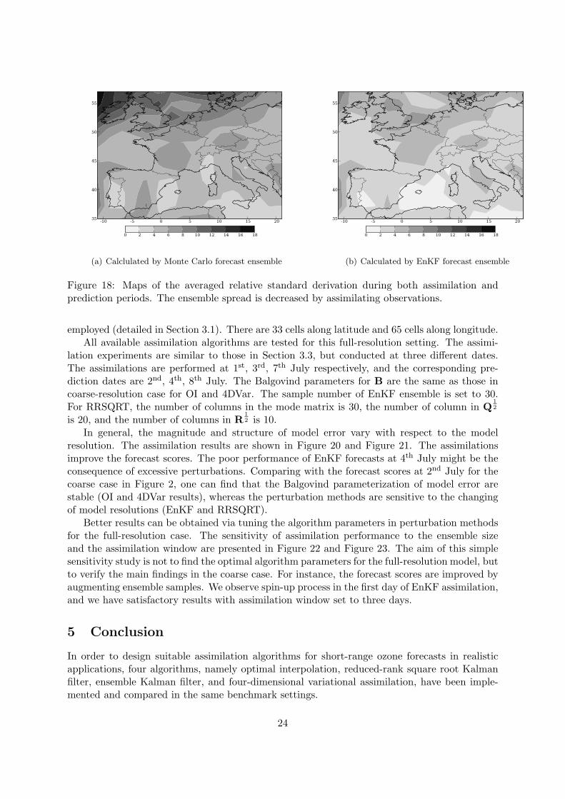
The ensemble relative standard derivations averaged over time are shown in Figure 18. Asexpected, the ensemble spread decreases when the assimilation is applied. One may notice highuncertainties around the coasts, although is not as clear as in Mallet and Sportisse [2006b] wherethe uncertainties were generated by statistics over several months. Our ensemble spread de-scribes an accidental uncertainty configuration that depends not only on the chemistry-transportprocesses, e.g. turbulence, but also on the meteorological scenarios.
4.4 Cycling Forecast for Coarse Case
It is expected that the findings in the previous sections are independent of the assimilationdates. To this end, we perform assimilation/prediction processes consecutively for one week.The length of the assim./predict. periods is chosen to be one day. The first assimilation periodis from 1st July 2001 at 01:00 UT to 2nd July at 00:00 UT, followed by the prediction from 2nd
July at 01:00 UT to 3rd July at 00:00 UT. The assimilation period of the second assim./predict.process is the same as the prediction period of the first assim./predict. process. The secondprediction period is from 3rd July at 01:00 UT to 4th July at 00:00 UT. The cycling continuesuntil the final assim./predict. process. The last prediction period is from 8th July at 01:00 UTto 9rd July at 00:00 UT. The initial conditions for the subsequent assimilation periods are thehourly forecasts based on previously controlled states after assimilations. The performance ofOI, EnKF and 4DVar forecasts over the prediction periods are shown in Figure 19.
The improvement of forecast performance with assimilation is obvious. The Balgovind pa-rameters for OI and 4DVar are constant, so are the perturbation magnitudes for the EnKFsamples. The lesser performance of 4DVar is probably due to the absence of model error duringassimilation. EnKF surpasses OI in forecasts longer than twelve hours. The approximation ofmodel error by refined perturbations is promising for longer forecasts.
4.5 Full-Resolution Case
The previous results are obtained with coarse models at a resolution of 2 × 2 × 1800s with3 vertical levels. In this section, the reference resolution at 0.5 × 0.5 × 600s with 5 levels is
22

0 10 20 30 4050
60
70
80
90
100
110
120
130
140St. Koloman (6, 12)
0 10 20 30 4030
40
50
60
70
80
90
100
110
120Heidenreichstein (6, 13)
0 10 20 30 4020
40
60
80
100
120
140
160Tanikon (6, 9)
0 10 20 30 4040
50
60
70
80
90
100
110
120Schmucke (7, 10)
0 10 20 30 400
20
40
60
80
100
120
140Niembro (4, 3)
0 10 20 30 400
20
40
60
80
100
120
140
160Revin (7, 7)
0 10 20 30 400
20
40
60
80
100
120Bottesford (8, 5)
0 10 20 30 4035
40
45
50
55
60
65
70
75Mace Head (9, 0)
0 10 20 30 4050
60
70
80
90
100
110
120
130Zarodnje (5, 13)
Figure 17: EnKF assimilation/prediction performances at nine stations. The titles read stationnames and their coordinates in model grid indices. The horizontal axis shows the accumulatedavailable observation numbers along time. Along vertical axis, the ozone concentrations areplotted in µg m−3. The diamond points show the observations, the short lines plot assimilatedconcentrations, and the lines with error bars are the means of the forecast ensemble. The errorbars are the relative standard derivations calculated with the forecast ensemble.
23
-10 -5 0 5 10 15 2035
40
45
50
55
0 2 4 6 8 10 12 14 16 18
(a) Calclulated by Monte Carlo forecast ensemble
-10 -5 0 5 10 15 2035
40
45
50
55
0 2 4 6 8 10 12 14 16 18
(b) Calculated by EnKF forecast ensemble
Figure 18: Maps of the averaged relative standard derivation during both assimilation andprediction periods. The ensemble spread is decreased by assimilating observations.
employed (detailed in Section 3.1). There are 33 cells along latitude and 65 cells along longitude.All available assimilation algorithms are tested for this full-resolution setting. The assimi-
lation experiments are similar to those in Section 3.3, but conducted at three different dates.The assimilations are performed at 1st, 3rd, 7th July respectively, and the corresponding pre-diction dates are 2nd, 4th, 8th July. The Balgovind parameters for B are the same as those incoarse-resolution case for OI and 4DVar. The sample number of EnKF ensemble is set to 30.For RRSQRT, the number of columns in the mode matrix is 30, the number of column in Q
1
2
is 20, and the number of columns in R1
2 is 10.In general, the magnitude and structure of model error vary with respect to the model
resolution. The assimilation results are shown in Figure 20 and Figure 21. The assimilationsimprove the forecast scores. The poor performance of EnKF forecasts at 4th July might be theconsequence of excessive perturbations. Comparing with the forecast scores at 2nd July for thecoarse case in Figure 2, one can find that the Balgovind parameterization of model error arestable (OI and 4DVar results), whereas the perturbation methods are sensitive to the changingof model resolutions (EnKF and RRSQRT).
Better results can be obtained via tuning the algorithm parameters in perturbation methodsfor the full-resolution case. The sensitivity of assimilation performance to the ensemble sizeand the assimilation window are presented in Figure 22 and Figure 23. The aim of this simplesensitivity study is not to find the optimal algorithm parameters for the full-resolution model, butto verify the main findings in the coarse case. For instance, the forecast scores are improved byaugmenting ensemble samples. We observe spin-up process in the first day of EnKF assimilation,and we have satisfactory results with assimilation window set to three days.
5 Conclusion
In order to design suitable assimilation algorithms for short-range ozone forecasts in realisticapplications, four algorithms, namely optimal interpolation, reduced-rank square root Kalmanfilter, ensemble Kalman filter, and four-dimensional variational assimilation, have been imple-mented and compared in the same benchmark settings.
24

03 Jul 04 Jul 05 Jul 06 Jul 07 Jul 08 Jul 09 Jul10
15
20
25
30
35
40
45
50
55R
MS
E
Forecast without assimilationOI forecastEnKF forecast4DVar forecast
Figure 19: The one-day forecast performances based on model simulations with/without assim-ilations in the context of cycling assimilation/predictions.
Reference OI EnKF 4DVar RRSQRT16
18
20
22
24
26
28
30
32
34
Fore
cast
score
s
2 July
4 July
8 July
Figure 20: Forecast scores of ozone concentrations during prediction dates.
25

02 Jul 03 Jul 04 Jul 05 Jul 06 Jul 07 Jul 08 Jul 09 Jul0
50
100
150
200
Con
cen
trati
on
s
ReferenceOIEnKFRRSQRT4DVarMeasurements
Figure 21: Time evolution of ozone forecasts against available observations at Montandon sta-tion.
30 50 80 110
Sample numbers
16
18
20
22
24
26
28
Fore
cast
score
s
Figure 22: Forecast scores at 2nd July against EnKF ensemble size.
26

1 2 3
Assimilation days
16
18
20
22
24
26
28
Fore
cast
score
s
Figure 23: EnKF forecast scores at 8th July against the number of assimilation days.
Although the forecasts beyond one day tend to approach the model simulations withoutassimilation (because of the low dependency of model simulations on initial conditions), it hasbeen shown that the assimilation algorithms significantly improve the ozone forecasts. Dataassimilation would be an indispensable part of practical ozone forecast systems as in NWP.
The comparison results have illustrated the limitations and potentials of different assimilationalgorithms. OI provides overall better performances. It benefits from the Balgovind parameteri-zation of model uncertainties during the assimilation periods. In EnKF, the model uncertaintieswere approximated by the statistics of the ensemble generated by perturbing uncertain modelparameters. This perturbation method shows good potential to alleviate the constraint of thelow dependency on initial conditions in ozone forecasts. EnKF produces best forecasts duringthe end of prediction periods. The strongly constrained 4DVar does a moderate job, becauseuncertainties are taken into account only at the initial date of the assimilation. Further studiesare needed, e.g. the estimation of ozone concentrations jointly with the emission rates [Elbernet al., 2007]. We remark that there are no final conclusions because of the unsettled formulationof model error. We paid less attention to RRSQRT, since, in our implementation, it is quitesimilar to EnKF.
We have also conducted sensitivity analysis on algorithm parameters, e.g. ensemble ran-domness and size, assimilation window, perturbation fields, and diverse model settings. Fur-ther refinements of the assimilation algorithms can thus be tested by tuning these algorithmparameters for better forecast performances. This is especially necessary for the case of thefull-resolution model.
It is the complexity of the chemistry-transport phenomena and the limited observationsthat make it difficult for the modeling and assimilation. The approximations of the complexphenomena make CTMs imperfect, and uncertainties arise. If a deterministic model is employed,or if the uncertainties are not realistic, the forecasts of the stable system approach to the referencesimulations without assimilation. Therefore all assimilation algorithms have to be adaptive, inone way or another, so that the uncertainties should be better represented.
For the design of better assimilation algorithms, serious investigations on error modelingare needed. The ensemble could be obtained from more uncertain sources, e.g. numericalapproximations and subgrid physical parameterizations. The statistics of the enlarged ensembleare expected to be more accurate approximations of the model error.
Spatially heterogeneous perturbations, which smooth out the spurious correlations of longdistance, would certainly produce more realistic model errors. Another concern is that the
27

lognormal perturbations might result in non-Gaussian model errors. In this case, assimilationmethods deviating from normal may have to be accounted for. Other methods rely on hybridiza-tions between sequential and variational methods which essentially use the assimilation resultsfrom both methods for error modeling. The comparison of ensemble forecast techniques [Malletand Sportisse, 2006a] and assimilation algorithms would also be an interesting topic for futurestudies.
References
R. Balgovind, A. Dalcher, M. Ghil, and E. Kalnay. A stochastic-dynamic model for the spatialstructure of forecast error statistics. Mon. Wea. Rev., 111(4):701–722, 1983.
M. Bocquet. Grid resolution dependence in the reconstruction of an atmospheric tracer source.Nonlinear Proc. Geoph., 12(2):219–233, 2005.
Jaouad Boutahar, Stephanie Lacour, Vivien Mallet, Denis Quelo, Yelva Roustan, and BrunoSportisse. Development and validation of a fully modular platform for numerical modellingof air pollution: POLAIR. Int. J. Env. and Pollution, 22(1/2):17–28, 2004.
F. Bouttier and P. Courtier. Data assimilation concepts and methods. Meteorological TrainingCourse Lecture Series, ECMWF, 1999.
Gerrit Burgers, Peter Jan van Leeuwen, and Geir Evensen. On the analysis scheme in theensemble Kalman filter. Mon. Wea. Rev., 126:1719–724, 1998.
R. H. Byrd, P. Lu, and J. Nocedal. A limited memory algorithm for bound constrained opti-mization. SIAM J. on Sci. and Stat. Comp., 16(5):1,190–1,208, 1995.
Gregory R. Carmichael, Adrian Sandu, Tianfeng Chai, Dacian N. Daescu, Emil M. Constan-tinescu, and Youhua Tang. Predicting air quality: Improvements through advanced meth-ods to integrate models and measurements. J. Comp. Phys., 227:3540 – 3571, 2008. doi:10.1016/j.jcp.2007.02.024.
T. Chai, G. R. Carmichael, Y. Tang, A. Sandu, M. Hardesty, P. Pilewskie, S. Whitlow, E.V.Browell, M.A. Avery, P. Nedelec, J.T. Merrill, A.M. Thompson, and E. Williams. Four-dimensional data assimilation experiments with international consortium for atmospheric re-search on transport and transformation ozone measurements. J. Geophys. Res., 112, 2007.doi: 10.1029/2006JD007763.
E.M. Constantinescu, T. Chai, A. Sandu, and G.R. Carmichael. Autoregressive models ofbackground errors for chemical data assimilation. J. Geophys. Res., 112:D12309, 2007a. doi:10.1029/2006JD008103.
E.M. Constantinescu, A. Sandu, T. Chai, and G.R. Carmichael. Ensemble-based chemical dataassimilation I: General approach. Quart. J. Roy. Meteor. Soc., 133(626):1229–1243, July2007b. ISSN 0035-9009. doi: 10.1002/qj.76.
R. Daley. Atmospheric data analysis. Combridge University Press, 1991.
H. Elbern and H. Schmidt. Ozone episode analysis by four-dimensional variational chemistrydata assimilation. J. Geophys. Res., 106(D4):3,569–3,590, 2001.
28

H. Elbern, A. Strunk, H. Schmidt, and O. Talagrand. Emission rate and chemical state estima-tion by 4-dimensional variational inversion. Atmos. Chem. Phys., 7(14):3749–3769, 2007.
Geir Evensen. The ensemble Kalman filter: Theoretical formulation and practical implementa-tion. Ocean Dynam., 53:343–367, 2003.
Geir Evensen. Sequential data assimilation with a nonlinear quasi-geostrophic model usingMonte Carlo methods to forecast error statistics. J. Geophys. Res., 99(C5):10,143–10,162,1994.
C. Faure and Y. Papegay. O∂yssee user’s guide – version 1.7. Technical Report 0224, INRIA,1998.
M. Fisher and D. J. Lary. Lagrangian four-dimensional variational data assimilation of chemicalspecies. Quart. J. Roy. Meteor. Soc., 121:1681–1704, 1995.
J. Flemming, M. van Loon, and R. Stern. Data assimilation for CTM based on optimum inter-polation and Kalman filter. paper presented at 26th NATO/CCMS International TechnicalMeeting on Air Pollution Modeling and Its Application, NATO Comm. on the Challenges ofthe Mod. Soc., Istanbul, 2003.
R. G. Hanea, G. J. M. Velders, and A. Heemink. Data assimilation of ground-level ozone inEurope with a Kalman filter and chemistry transport model. J. Geophys. Res., 109, 2004.
Steven R. Hanna, Joseph C. Chang, and Mark E. Fernau. Monte Carlo estimates of uncertain-ties in predictions by a photochemical grid model (UAM-IV) due to uncertainties in inputvariables. Atmos. Env., 32(21):3,619–3,628, 1998.
Steven R. Hanna, Zhigang Lu, H. Christopher Frey, Neil Wheeler, Jeffrey Vukovich, SaravananArunachalam, Mark Fernau, and D. Alan Hansen. Uncertainties in predicted ozone concen-trations due to input uncertainties for the UAM-V photochemical grid model applied to theJuly 1995 OTAG domain. Atmos. Env., 35(5):891–903, 2001.
A. W. Heemink, M. Verlaan, and A. J. Segers. Variance reduced ensemble Kalman filtering.Mon. Wea. Rev., 129:1,718–1,728, 2001.
J. Hoelzemann, H. Elbern, and A. Ebel. PSAS and 4DVar data assimilation for chemical stateanalysis by urban and rural observation sites. Phys. Chem. Earth, 26:807–812, 2001.
Larry W. Horowitz, Stacy Walters, Denise L. Mauzerall, Louisa K. Emmons, Philip J. Rasch,Claire Granier, Xuexi Tie, Jean-Francois Lamarque, Martin G. Schultz, Geoffrey S. Tyndall,John J. Orlando, and Guy P. Brasseur. A global simulation of tropospheric ozone and relatedtracers: description and evaluation of MOZART, version 2. J. Geophys. Res., 108(D24), 2003.
E. Kalnay. Atmospheric modeling, data assimilation and predictability. Cambridge Univ. Press,2003.
E. Kalnay, H. Li, T. Miyoshi, S.-C. Yang, and J. Ballabrera. 4DVar or ensemble Kalman filter.Tellus A, 59A:758–773, 2007.
F.-X. Le Dimet and V.P. Shutyaev. On deterministic error analysis in variational data assimi-lation. Nonlinear Proc. Geoph., 12(4):481–490, May 2005.
Francois-Xavier Le Dimet and Olivier Talagrand. Variational algorithms for analysis and assim-ilation of meteorological observations: theoretical aspects. Tellus A, 38A:97–110, 1986.
29
X. S. Liang and R. Kleeman. Information transfer between dynamical system components. Phys.
Rev. Lett., 95(24):244101, 2005.
Andrew C. Lorenc. The potential of the ensemble Kalman filter for NWP - a comparison with4DVar. Quart. J. Roy. Meteor. Soc., 129(595):3,183–3,203, 2003.
Jean-Francois Louis. A parametric model of vertical eddy fluxes in the atmosphere. Boundary-
Layer Meteor., 17:187–202, 1979.
Vivien Mallet and Bruno Sportisse. Ensemble-based air quality forecasts: A multimodel ap-proach applied to ozone. J. Geophys. Res., 111(D18), 2006a.
Vivien Mallet and Bruno Sportisse. Uncertainty in a chemistry-transport model due to physicalparameterizations and numerical approximations: An ensemble approach applied to ozonemodeling. J. Geophys. Res., 111(D1), 2006b.
Vivien Mallet, Denis Quelo, Bruno Sportisse, Meryem Ahmed de Biasi, Edouard Debry, IreneKorsakissok, Lin Wu, Yelva Roustan, Karine Sartelet, Marilyne Tombette, and Hadjira Foud-hil. Technical Note: The air quality modeling system Polyphemus. Atmos. Chem. Phys., 7(20):5,479–5,487, 2007.
Paulette Middleton, William R. Stockwell, and William P. L. Carter. Aggregation and analysis ofvolatile organic compound emissions for regional modeling. Atmos. Env., 24A(5):1,107–1,133,1990.
C. Pires, R. Vautard, and O. Talagrand. On extending the limits of variational assimilation innonlinear chaotic systems. Tellus A, 48A:96–121, 1996.
Arjo Segers. Data assimilation in atmospheric chemistry models using Kalman filtering. PhDthesis, Delft University, 2002. www.library.tudelft.nl.
D. Simpson, W. Winiwarter, G. Borjesson, S. Cinderby, A. Ferreiro, A. Guenther, C. N. Hewitt,R. Janson, M. A. K. Khalil, S. Owen, T. E. Pierce, H. Puxbaum, M. Shearer, U. Skiba,R. Steinbrecher, L. Tarrason, and M. G. Oquist. Inventorying emissions from nature inEurope. J. Geophys. Res., 104(D7):8,113–8,152, 1999.
W. R. Stockwell, P. Middleton, J. S. Chang, and X. Tang. The second generation regional aciddeposition model chemical mechanism for regional air quality modeling. J. Geophys. Res., 95(D10):16,343–16,367, 1990.
William R. Stockwell, Frank Kirchner, Michael Kuhn, and Stephan Seefeld. A new mechanismfor regional atmospheric chemistry modeling. J. Geophys. Res., 102(D22):25,847–25,879, 1997.
I.B. Troen and L. Mahrt. A simple model of the atmospheric boundary layer; sensitivity tosurface evaporation. Boundary-Layer Meteor., 37:129–148, 1986.
J. G. Verwer, W. Hundsdorfer, and J. G. Blom. Numerical time integration for air pollutionmodels. Surveys on Math. for Indus., 10:107–174, 2002.
M. L. Wesely. Parameterization of surface resistances to gaseous dry deposition in regional-scalenumerical models. Atmos. Env., 23:1,293–1,304, 1989.
L. Zhang, J. R. Brook, and R. Vet. A revised parameterization for gaseous dry deposition inair-quality models. Atmos. Chem. Phys., 3:2,067–2,082, 2003.
30