a comparison of the heft subsurface and … · a comparison of the heft subsurface and delfic...
TRANSCRIPT

A COMPARISON OF THE HEFT SUBSURFACE AND DELFIC PARTICLE SIZE DISTRIBUTIONS
AND EFFECTS IN HPAC
THESIS
Eric T. Skaar, First Lieutenant, USAF
AFIT/GNE/ENP/05-13
DEPARTMENT OF THE AIR FORCE AIR UNIVERSITY
AIR FORCE INSTITUTE OF TECHNOLOGY
Wright-Patterson Air Force Base, Ohio
APPROVED FOR PUBLIC RELEASE: DISTRIBUTION IS UNLIMITED

The views expressed in this thesis are those of the author and do not reflect the official policy or position of the United States Air Force, Department of Defense, or the United States Government.

AFIT/GNE/ENP/05-13
A COMPARISON OF THE HEFT SUBSURFACE
AND DELFIC PARTICLE SIZEDISTRIBUTIONS
AND EFFECTS IN HPAC
THESIS
Presented to the Faculty
Department of Engineering Physics
Graduate School of Engineering and Management
Air Force Institute of Technology
Air University
Air Education and Training Command
In Partial Fulfillment of the Requirements for the
Degree of Master of Science in Nuclear Engineering
Eric T. Skaar, BS
First Lieutenant, USAF
March 2005
APPROVED FOR PUBLIC RELEASE; DISTRIBUTION IS UNLIMITED.


AFIT/GNE/ENP/05-13
Abstract
The Heft subsurface three component lognormal fallout particle size distribution
is compared and contrasted with the single lognormal fallout particle size distribution
used by the Defense Land Fallout Interpretive Code (DELFIC). Comparison of the two
distributions is accomplished with results from the AFIT smear code and the Hazard
Prediction and Assessment Capability (HPAC). The effect of the distributions is
explored in HPAC for varying yield weapons, varying surfaces, precipitation conditions,
varying wind effects and varying dose rate times. The results from the two distributions
are quantitatively compared using the concepts of grounded source normalization
constant and the rate at which activity is being deposited on the ground everywhere at
time t.
The Heft subsurface three component lognormal fallout particle size distribution
results in significantly less activity on the ground than does the DELFIC single lognormal
particle size distribution. The grounded source normalization constant resulting from the
Heft distribution is up to three times smaller than that observed when using the DEFLIC
distribution.
iv

Acknowledgments
I would like to thank my advisor, Dr. Charles J. Bridgman for his time, criticism,
encouragement and humor. It has been an honor and a privilege to work under his
tutelage. I’d also like to thank the members of my thesis committee, Lt. Col Vincent
Jodoin and Lt Col Steve Fiorino for their feedback.
I am also indebted to all of those who went out of their way to help me,
particularly Dr. Joseph T. McGahan and Major D. Brent Morris. Without their insight
and assistance I could not have completed this thesis. A special thanks also to Major
Steven Weber who helped me in the writing and editing of this thesis. Eric T. Skaar
v

Table of Contents
Page Abstract ...................................................................................................................... iv Acknowledgements........................................................................................................v List of Figures .......................................................................................................... viii List of Tables ............................................................................................................ xii I. Introduction ............................................................................................................1 Motivation...............................................................................................................1 Background.............................................................................................................1 Problem...................................................................................................................2 Scope.......................................................................................................................3 General Approach ...................................................................................................3 II. Literature Review...................................................................................................4 Physics of Fallout Formation .................................................................................4 Description of the DELFIC Particle Distribution ..................................................7 Description of the Heft Subsurface Particle Distribution ......................................9 Comparison of the Heft Subsurface Crystalline Distribution with the Baker Airburst Distribution............................................................................................10 Comparison of the Heft Three-Component Subsurface Distribution with the DELFIC Surface Distribution..............................................................................11 HPAC Overview ..................................................................................................12 Cloud Rise in Newfall/DELFIC...........................................................................13 Activity Calculation in DELFIC..........................................................................15 Basic Information Concerning SCIPUFF ............................................................19 III. Methodology 23 Introduction to Source Normalization Constant, k ..............................................23 Method for Calculating Source Normalization Constant from HPAC Output ....24 Introduction to g(t)...............................................................................................25 Method for Calculating the Function g(t) from HPAC Outputs ..........................27 General Information Concerning HPAC Runs ....................................................27 IV. Results and Data Comparison.............................................................................31 Results of the AFIT Smear Code for DELFIC Surface and Heft Subsurface Particle Distributions ...........................................................................................31
vi

A Comparison of the DELFIC and Heft Subsurface Particle Distributions for Varying Yields and Resolutions ..........................................................................39 Variation in the Grounded Source Normalization Constant When Computed from Different Late Time Dose Rates .................................................................48 V. Interaction of Particle Size Distribution with Other Variable Parameters in HPAC...................................................................................................................58 Effects of Varying Surfaces .................................................................................58 Effects of Rain Out ..............................................................................................67 Effects of Different Constant Wind Speeds for DELFIC and Heft Three Component Particle Distributions........................................................................76 VI. Research Summary and Conclusions..................................................................81 Research Summary ..............................................................................................81 Conclusions..........................................................................................................81 Recommendations for Future Research ...............................................................83 Glossary .....................................................................................................................86
Appendix A. Converting a Log10 distribution to a Ln Distribution ...........................89 Appendix B: Summarization of Freiling Ratios and Heft Distributions......................91 Appendix C. Summary of Surface Effects in SCIPUFF ..........................................105 Appendix D. Code for Calculating g(t) ....................................................................111 Appendix E. Code for Calculating the Effective Source Normalization Constant ..122 Bibliography ............................................................................................................134
vii

List of Figures
Figure Page
1. DELFIC Number Distribution ...........................................................................8
2. DELFIC Mass Distribution................................................................................8
3. Volume Distribution for Heft Subsurface Crystalline and Baker Airburst......11
4. Comparison of DELFIC and Heft Three-Component Mass Distributions ......12
5. HPAC Stages (11:4-1) .....................................................................................13
6. Nuclear Weapon Parameters Used in HPAC Runs..........................................28
7. Fixed Wind Parameters Used in HPAC Runs..................................................29
8. General Weather Parameters Used in HPAC Runs .........................................29
9. Typical HPAC Dose Rate Contour with Default Dose Rate Values Shown in Legend .........................................................................................................30
10. AFIT Smear Code 30 Day Dose Contour for 1kt Surface Burst using
DELFIC Distribution with 10kph Constant wind (Units in Roentgen) ...........33
11. AFIT Smear Code 30 Day Dose Contour for 1kt Surface Burst using Heft Subsurface Distrubution with 10kph Constant Wind (Units in Roentgen)......34
12. AFIT Smear Code 30 Day Dose Contour for 1kt Surface Burst using
Crystalline Distribution with 10kph Constant Wind (Units in Roentgen).......35
13. AFIT Smear Code 30 Day Dose Contour for 1kt Surface Burst using Glass Distribution with 10kph Constant Wind (Units in Roentgen) .........................36
14. AFIT Smear Code 30 Day Dose Rate for 1kt Surface Burst using the Local
Distribution with 10kph Constant Wind (Units in Roentgen) .........................37
15. G(t) Comparison for 1kt Surface Burst using Heft Subsurface and DELFIC Particle Distributions in AFIT Smear Code.....................................................38
16. Altitudes of the Stabilized Cloud Top and Cloud Bottom Based on Yield
for Surface Bursts (9: 431)...............................................................................39
viii

17. HPAC 4.03 Dose Rate Contour for 1kt Surface Burst at 12.75 Hours............40
18. HPAC 4.04 Dose Rate Contour for 1kt Surface Burst at 12.25 Hours............40
19. HPAC 4.03 Ground Zero Dose Rate Contour for 1kt Surface Burst at 12 Hours................................................................................................................41
20. HPAC 4.04 Ground Zero Dose Rate Contour for 1kt Surface Burst at 12
Hours................................................................................................................42
21. g(t) for 1kt Surface Burst in HPAC 4.03 and 4.04...........................................43
22. HPAC 4.03 Dose Rate Contour for 10kt Surface Burst at 23 Hours...............45
23. HPAC 4.04 Dose Rate for 10kt Surface Burst at 22 Hours .............................45
24. HPAC 4.03 Dose Rate Contour for 100kt Surface Burst at 48 Hours.............46
25. HPAC 4.04 Dose Rate Contour for 100kt Surface Burst at 48 Hours.............47
26. Dose Rate vs. Time (Dashed Line Represents the Way-Wigner Approximation) (9:392) ...................................................................................49
27. HPAC 4.03 Dose Rate Contour for 100kt Surface Burst at 8 Hours...............50
28. HPAC 4.03 Dose Rate Contour for 100kt Surface Burst at 16 Hours.............50
29. HPAC 4.03 Dose Rate Contour for 100kt Surface Burst at 24 Hours.............50
30. HPAC 4.03 Dose Rate for 100kt Surface Burst at 32 Hours ...........................50
31. HPAC 4.03 Dose Rate Contour for 100kt Surface Burst at 40 Hours.............50
32. HPAC 4.03 Dose Rate Contour for 100kt Surface Burst at 48 Hours.............50
33. HPAC 4.04 Dose Rate Contour for 100kt Surface Burst at 8 Hours...............51
34. HPAC 4.04 Dose Rate Contour for 100kt Surface Burst at 16 Hours.............51
35. HPAC 4.04 Dose Rate Contour for 100kt Surface Burst at 24 Hours.............51
36. HPAC 4.04 Dose Rate Contour for 100kt Surface Burst at 32 Hours.............51
37. HPAC 4.04 Dose Rate Contour for 100kt Surface Burst at 40 Hours.............51
ix

38. HPAC 4.04 Dose Rate Contour for 100kt Surface Burst at 48 Hours.............51
39. HPAC 4.03 Dose Rate Contour for 1kt Surface Burst at 4 Hours...................55
40. HPAC 4.03 Dose Rate Contour for 1kt Surface Burst at 8 Hours...................55
41. HPAC 4.03 Dose Rate Contour for 1kt Surface Burst at 12 Hours.................55
42. HPAC 4.03 Dose Rate Contour for 1kt Surface Burst at 12.75 Hours............55
43. HPAC 4.04 Dose Rate Contour for 1kt Surface Burst at 4 Hours...................56
44. HPAC 4.04 Dose Rate Contour for 1kt Surface Burst at 8 Hours...................56
45. HPAC 4.04 Dose Rate Contour for 1kt Surface Burst at 12 Hours.................56
46. HPAC 4.04 Dose Rate Contour for 1kt Surface Burst at 12.25 Hours............56
47. HPAC 4.03 Dose Rate Contour for 1kt Surface Burst with Cultivated Surface at 12 Hours..........................................................................................59
48. HPAC 4.04 Dose Rate Contour for 1kt Surface Burst with Cultivated
Surface at 12 Hours..........................................................................................59
49. HPAC 4.03 Dose Rate Contour for 1kt Surface Burst with Forest Surface at 12 Hours.......................................................................................................61
50. HPAC 4.04 Dose Rate Contour for 1kt Surface Burst with Forest Surface
at 12 Hours.......................................................................................................61
51. HPAC 4.03 Dose Rate Contour for 1kt Surface Burst with Urban Suface at 12 Hours.......................................................................................................62
52. HPAC 4.04 Dose Rate Contour for 1kt Surface Burst with Urban Surface
at 12 Hours.......................................................................................................62
53. HPAC 4.03 Dose Rate Contour for 1kt Surface Burst with Grassland Surface at 12 Hours..........................................................................................63
54. HPAC 4.04 Dose Rate Contour for 1kt Surface Burst with Grassland
Surface at 12 Hours..........................................................................................63
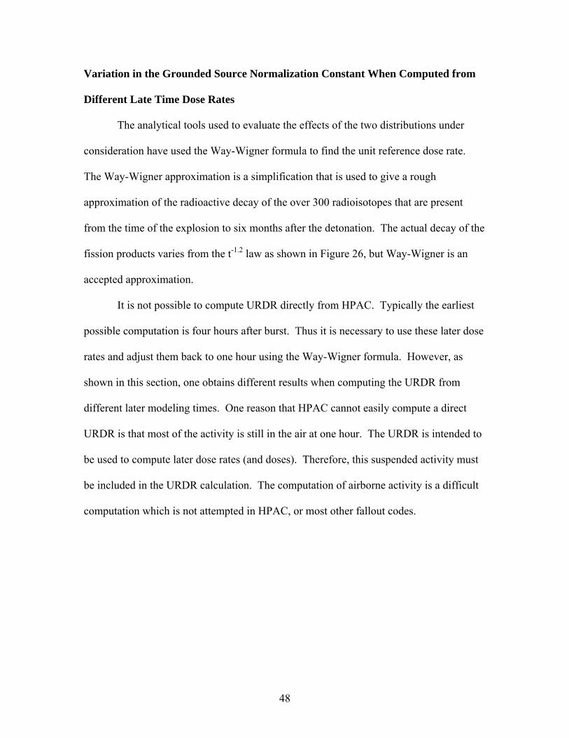
55. HPAC 4.03 Dose Rate Contour 1kt Surface Burst with Desert Surface at 12 Hours...........................................................................................................64
x

56. HPAC 4.04 Dose Rate Contour for 1kt Surface Burst with Desert Surface
at 12 Hours.......................................................................................................64
57. HPAC 4.03 Dose Rate Contour for 1kt Surface Burst with Water Surface at 12 Hours.......................................................................................................65
58. HPAC 4.04 Dose Rate Contour for 1kt Surface Burst with Water Surface
at 12 Hours.......................................................................................................65
59. HPAC 4.03 Dose Rate Contour for 1kt Surface Burst with No Rain ..............72
60. HPAC 4.03 Dose Rate Contour for 1kt Surface Burst with Light Rain at 12 Hours................................................................................................................72
61. HPAC 4.03 Dose Rate Contour 1kt Surface Burst with Heavy Rain at 12
Hours................................................................................................................72
62. HPAC 4.04 Dose Rate Contour for 1kt Surface Burst with No Rain at 12 Hours................................................................................................................72
63. HPAC 4.04 Dose Rate Contour for 1kt Surface Burst with Light Rain at
12 Hours...........................................................................................................72
64. HPAC 4.04 Dose Rate Contour for 1kt Surface Burst with Heavy Rain at 12 Hours...........................................................................................................72
65. HPAC 4.03 Dose Rate Contour for 10kt Surface Burst with No Rain at 23
Hours................................................................................................................74
66. HPAC 4.03 Dose Rate Contour for 10kt Surface Burst with Light Rain at 23 Hours...........................................................................................................74
67. HPAC 4.03 Dose Rate Contour for 10kt Surface Burst with Heavy Rain at
23 Hours...........................................................................................................74
68. HPAC 4.04 Dose Rate Contour for 10kt Surface Burst with No Rain at 22 Hours................................................................................................................74
69. HPAC 4.04 Dose Rate Contour for 10kt Surface Burst with Light Rain at
22 Hours...........................................................................................................74
70. HPAC 4.04 Dose Rate Contour for 10kt Surface Burst with Heavy Rain at 22 Hours...........................................................................................................74
xi

71. HPAC 4.03 Dose Rate Contour for 1kt Surface Blast with 5kph Constant Wind.................................................................................................................77
72. HPAC 4.03 Dose Rate Contour for 1kt Surface Burst with 10kph Constant
Wind.................................................................................................................77
73. HPAC 4.03 Dose Rate Contour for 1kt Surface Burst with 15kph Constant Wind.................................................................................................................77
74. HPAC 4.04 Dose Rate Contour for 1kt Surface Burst with 5kph Constant
Wind.................................................................................................................78
75. HPAC 4.04 Dose Rate Contour for 1kt Surface Burst with 10kph Constant Wind.................................................................................................................78
76. HPAC 4.04 Dose Rate Contour for 1kt Surface Burst with 15kph Constant
Wind.................................................................................................................78
77. G(t) Comparison for HPAC 4.03 1kt Surface Burst with Different Winds.....80
78. G(t) Comparison for HPAC 4.04 1kt Surface Burst with Different Winds.....80
79. Freiling Ratios for Land Surface Detonation Fallout Particles........................95
80. Specific Activity vs Mean Particle Diameter...................................................97
81. Mass Distribution for Heft Two-Component Surface Burst Fallout Particles............................................................................................................98
82. Modified Freiling Plot for 137Cs from Aerial Filters of Surface Burst ..........100
83. Mass Distribution for Heft Three-Component Surface Burst Fallout Particles..........................................................................................................101
84. Volatile Distribution for Heft Tri-Component Surface Burst Fallout
Particles..........................................................................................................103
85. Refractory Distribution for Heft Tri-Component Subsurface Burst Fallout Particles..........................................................................................................103
xii
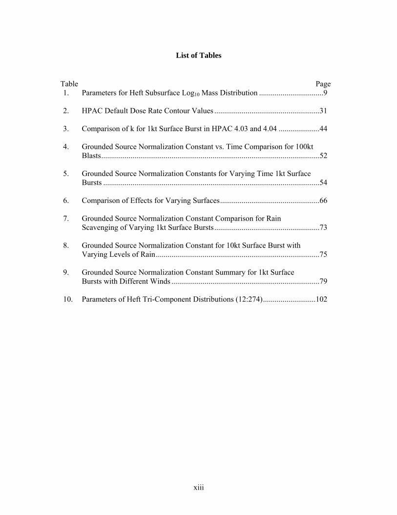
List of Tables
Table Page 1. Parameters for Heft Subsurface Log10 Mass Distribution .................................9
2. HPAC Default Dose Rate Contour Values ......................................................31
3. Comparison of k for 1kt Surface Burst in HPAC 4.03 and 4.04 .....................44
4. Grounded Source Normalization Constant vs. Time Comparison for 100kt Blasts................................................................................................................52
5. Grounded Source Normalization Constants for Varying Time 1kt Surface
Bursts ...............................................................................................................54
6. Comparison of Effects for Varying Surfaces...................................................66
7. Grounded Source Normalization Constant Comparison for Rain Scavenging of Varying 1kt Surface Bursts......................................................73
8. Grounded Source Normalization Constant for 10kt Surface Burst with
Varying Levels of Rain....................................................................................75
9. Grounded Source Normalization Constant Summary for 1kt Surface Bursts with Different Winds ............................................................................79
10. Parameters of Heft Tri-Component Distributions (12:274)...........................102
xiii

A COMPARISON OF THE HEFT SUBSURFACE AND DELFIC PARTICLE SIZE
DISTRIBUTIONS AND EFFECTS IN HPAC
I. Introduction
Motivation
The possibility of a domestic nuclear event due to rogue nations or transnational
threats demands vigilance from our law enforcement, intelligence and military
communities to protect the citizens of this country from that danger. In order to assist
these diverse groups, the scientific community has an obligation to understand the nature
of the threat posed by nuclear weapons and the impacts that would result from a nuclear
detonation.
The nuclear tests conducted in the 40’s, 50’s, and 60’s have left us with a wealth of
scientific knowledge concerning the effects of nuclear weapons. However, despite this
vast amount of data, our ability to model the effects of a nuclear event is limited by our
finite understanding of its physics, our imperfect mathematical tools used to describe the
physics that we do understand, and our limited computational resources. Our limited
computational ability requires that we greatly simplify the mathematics used to analyze
nuclear events. As such, we strive to find the best mathematical representation of
physical phenomena that gives us an understanding of what is happening without being
overly complicated or time consuming.
Background
In order to mathematically represent a chemical, biological, radiological or
1
nuclear (CBRN) event, the Defense Threat Reduction Agency (DTRA) has overseen the
development and maintenance of the Hazard Prediction and Assessment Capability
(HPAC) software. HPAC is a modeling program that attempts to predict the effects from
a CBRN event. HPAC is used for planning purposes by military strategists and
emergency response personnel.
All fallout codes consist of two basic components: source definition and transport.
Source definition takes into account all the variables from the moment of detonation
through cloud rise until the formation of the stabilized nuclear cloud. Transport then
takes the fallout defined in the stabilized nuclear cloud and uses weather and deposition
phenomena to distribute the fallout over the ground. This will be described in greater
detail in Chapter 3.
A single lognormal was suggested by the Defense Land Fallout Interpretative Code
(DELFIC) to model the particle size range of fallout particles for surface bursts (19:16).
A surface burst is a nuclear explosion where the fireball interacts with the surface of the
earth. This single lognormal has been traditionally used to represent the particle size
distribution typical of fallout that results from nuclear bursts in many subsequent fallout
codes including HPAC. In 1968, Heft proposed a series of three lognormal distributions
to represent the particle size distribution that would result from a subsurface nuclear
detonation (12:271). Thanks to the work of McGahan of SAIC, the Heft subsurface tri-
lognormal particle distribution has been incorporated into the most recent version of
HPAC, HPAC 4.04 (14:1). All versions of HPAC previous to 4.04 use the DELFIC
single-lognormal to model the particle size distribution from a nuclear burst.
Problem
This thesis compares and contrasts the Heft distribution with the DELFIC distribution
in order to quantitatively and qualitatively describe the effects of the two particle
distributions on the predictive fallout contours of HPAC.
2
Scope
HPAC can be used to model a variety of CBRN scenarios. HPAC can model
subsurface, surface and near-surface nuclear blasts up to 10 megatons. This research
looks specifically at the differences between predictions of HPAC 4.03 and 4.04
generated by the nuclear weapon module as a result of differing particle size
distributions. While cloud rise dynamics play an important role in fallout prediction, it is
not considered here. Similarly, the discussion of HPAC’s transport module, SCIPUFF, is
limited to explanation as it pertains to fallout particle deposition and a brief critique of
rain scavenging mechanisms in SCIPUFF. Validation of the accuracy of the fallout
modeling by comparison with actual nuclear surface bursts is not considered here. For a
more complete treatment of this subject please see “A Comparison of Hazard Prediction
and Assessment Capability (HPAC) Software Dose Rate Contour Plots to a Sample of
Local Fallout Data from Test Detonations in the Continental United States, 1945-1962”
by Richard Chancellor (4).
General Approach
This research begins with a discussion of the physics of fallout formation. First,
emphasis is placed upon the concept of Freiling ratio and its implications for
determination of radionuclide distribution in fallout particles. Next, particle distributions
are considered with a focus on describing the DELFIC single lognormal and the Heft tri-
lognormal particle size distributions. After this, a brief overview of HPAC is given with
emphasis on particle distributions HPAC uses to model fallout particle sizes. Finally, the
impact of the two particle distributions is considered on varying weapon yields,
resolutions, surfaces, rainout and winds.
3

II. Literature Review
This chapter provides a brief overview of the physics of fallout formation and a
brief description of the DELFIC and Heft subsurface distributions. Finally, an overview
of HPAC is provided with a summary of how components of the nuclear weapons and
transport module are calculated.
Physics of Fallout Formation
When a nuclear weapon is detonated the fission of fuel atoms (either 235U or
239Pu) causes a great deal of energy to be released in a very short amount of time. This
release of energy translates into a dramatic increase in temperature and pressure. The
energy translated into heat is referred to as thermal radiation and the visible light given
off from a nuclear explosion is referred to as the fireball. The temperature of a nuclear
explosion can reach up to tens of millions of degrees. Matter that interacts with this high
temperature within the fireball is vaporized. After the moment of detonation, the
temperature causes the fireball to rise after the pressure comes in to equilibrium with its
surroundings during fireball expansion. The aforementioned expansion results in a
temperature drop within the fireball (8:26-44).
At a bare minimum, debris from the weapon itself is present in the fireball of a
nuclear explosion. This debris includes casing and components from the weapon itself as
well as radioisotopes from the nuclear fuel of the weapon. These radioisotopes will
include both unused atoms of either uranium or plutonium as well as radioisotopes that
are the result of fission products or decay from fission products. However, since both
235U and 239Pu have relatively long half lives, we are primarily concerned with the
activity of the fission products, which have much shorter half lives.
4

In the case of a surface burst the fireball interacts with the ground. As the fireball
rises, it draws up soil from the surface below. As the soil interacts with the fireball it is
vaporized. Eventually, the fireball cools to the boiling point of the local soil material.
When this boiling point is reached, soil material starts to condense together. This
particular temperature varies based on the atomic composition of the soil. The
temperature within the fireball continues to fall below the boiling point of the local soil.
When the fireball temperature reaches the melting point of the soil, the soil particles start
to solidify (20:3-5). The melting point is generally assumed to be around 1400ºC (6:3).
As the soil material starts to condense, radioisotopes from the weapon start to
condense onto the soil. The fission products do not condense onto each other because of
the relative abundance of the soil material in comparison with the fission products.
Fission fragments make up a very small proportion of the mass of debris in a nuclear
explosion. The fraction of fission fragments in a surface burst will be in the range of
parts per ten million (2:402). For this reason, the soil acts as a carrier for the fission
product radioisotopes. Similar to the soil material, the temperature at which a fission
product radioisotope will condense varies. Some radioisotopes have a condensation
temperature that is greater than the melting temperature of the carrier soil material.
Consequently, when the temperature of the fireball reaches the condensation temperature
of the carrier soil material, these radioisotopes immediately begin to condense onto the
carrier soil. These radioisotopes are known as refractories. Because refractories
condense onto carrier while it is still molten and condensing, they have the opportunity to
both condense with the carrier and diffuse throughout the volume of the soil particle. For
this reason, refractories tend to be volume distributed within the condensed soil particles.
5

Conversely, radioisotopes that have boiling temperatures lower than the
solidification point of the local soil, and hence condense at temperatures lower than the
melting point of the local carrier material, are known as volatiles. Volatiles do not
condense onto the local soil particles until the soil particles have formed and solidified.
As a result of this, volatiles are surface distributed over the soil particles (6:3).
The relative abundance of different radioisotopes found in fallout particles varies
based on many factors. One of these factors is the size of the fallout particles. Fallout
particle size ranges from a few tenths of a micron to 1 millimeter or more. The first
particles to be formed grow larger than particles formed at later times. As such, they
scavenge the refractory radioisotopes which condense at a higher temperature, and hence
form at a time sooner than the volatiles. When these early forming particles get large
enough they fall out of the fireball and onto the earth. These early fallout particles often
leave the fireball before it has cooled enough for certain volatiles to condense onto them.
As such, they are refractory rich and volatile poor. Smaller soil particles, however, are
often introduced into the nuclear fireball at a later time and may not even be melted
depending on the temperature of the fireball at the time of their introduction. Because
these smaller particles are formed at a later time, most of the refractories have already
been scavenged and as a result, these smaller particles collect more volatiles.
Fractionation is then the difference in the radioisotopic composition of fallout particles
from the overall composition of fission fragments or as Freiling defines it, “any alteration
of radionuclide composition occurring between the time of detonation and the time of
radiochemical analysis which causes the debris sample to be nonrepresentative of the
detonation products taken as a whole” (7:1991).
6

7
Description of the DELFIC Particle Distribution
The DELFIC lognormal particle distribution for surface bursts is given by the
following equation:
20)ln(
21
21)(
⎥⎦
⎤⎢⎣
⎡ −−
= βα
βπ
d
ed
df (1)
where,
f(d) is the fraction of particles with diameter d
β is the natural logarithm of the standard deviation (ln(4.0))
α B0B is the natural logarithm of the median diameter in microns (ln(0.407)) (19:16).
Two implicit assumptions of most particle distributions are that the fallout
particles are spherical and they have a constant density across the entire distribution.
One fortunate property of the lognormal number distribution is the relative ease of
finding the surface area and volume distributions from the number distribution. The
surface area distribution can be found by substituting αB0 B with α B2B where 202 2βαα += .
The volume distribution can be found by substituting αB0 B with α B3B where
203 3βαα += (2:405-406). It should be noted that volume and mass distributions are
equivalent for spherical particles with constant densities over the distribution.
As seen in Figure 2, most of the mass contained in the distribution is to be found
above 100 microns. Since volume distribution is assumed for larger particles (19:50),
most of the activity will be found in this range as well.

0
0.2
0.4
0.6
0.8
1
1.2
1.4
1.6
1.8
2
0.01 1.01 2.01 3.01 4.01 5.01 6.01
Diameter (Microns)
Perc
ent N
umbe
r
Figure 1: DELFIC Number Distribution
In terms of numbers of particles, 99% of fallout particles, according to the
DELFIC number distribution shown in Figure 1, are found below 10 microns.
0
0.001
0.002
0.003
0.004
0.005
0.006
0.007
1 10 100 1000 10000
Diameter (microns)
Volu
me
Perc
ent
Figure 2: DELFIC Mass Distribution
8

9
Description of the Heft Subsurface Particle Distribution
The Heft subsurface mass distribution is given by the following equation:
∑= ⎥
⎥
⎦
⎤
⎢⎢
⎣
⎡
⎟⎟⎠
⎞⎜⎜⎝
⎛ −−⎟
⎟⎠
⎞⎜⎜⎝
⎛=
3
1
2
2exp
2i i
i
i
im xxdx
dFσπσ
φ (2)
where
iφ is the percentage of mass for the iP
thP population
σ Bi B is the standard deviation of the logB10B(diameter) for the iP
thP population
iχ is the logB10 B of the average diameter in microns for the iP
thP population
χ is the logB10B of the diameter in microns (12:274).
The parameters for equation 5 are shown below in Table 1.
Table 1: Parameters for Heft Subsurface LogB10B Mass Distribution
Population iφ σ Bi B
iχ
1 (Local) 0.40 0.57 2.48
2 (Glass) 0.474 0.23 1.26
3 (Crystalline) 0.126 0.28 0.83
The Heft subsurface distribution can be converted from a lognormal base 10
distribution to a lognormal base e distribution (see Appendix A). This results in the
following formula:
∑=
⎥⎦
⎤⎢⎣
⎡ −−
=3
1
)ln(21 0
2)(
i
d
i
i i
i
ed
df βα
βπφ
(3)

10
where
Population iφ β Bi B α B0B α B3B
1 (Local) 0.40 1.31 0.542 5.71
2 (Glass) 0.474 0.5296 2.06 2.9
3 (Crystalline) 0.126 0.6447 0.6699 1.92
Comparison of Heft Subsurface Crystalline Distribution with Baker Airburst
Distribution
For an airburst, Baker suggests a single lognormal distribution with a Beta equal
to ln(2) and the median radius of 0.1 microns (2:404). This is shown along with the Heft
subsurface crystalline component in Figure 3.
It can be seen from figure Figure 3 that while the crystalline particles are larger as
a whole, there is considerable overlap between the airburst and the crystalline component.
Even though Baker’s small distribution assumes no carrier soil whatsoever, there is some
similarity between the Baker small distribution and the Heft subsurface crystalline
distribution. This means the transport of fallout particles due to the crystalline
component will behave similarly to transport of fallout particles from an airburst. Since
an airburst produces no local fallout, it is not an unreasonable expectation that the

0
0.2
0.4
0.6
0.8
1
1.2
1.4
1.6
1.8
2
0 5 10 15 20 25
Diameter (microns)
dNw
/dd Baker
Airburst
Heft Subsurface Crystalline Distribution
Figure 3: Volume Distribution for Heft Subsurface Crystalline and Baker Airburst
crystalline portion of the Heft three-component subsurface distribution will not contribute
significant amounts of activity to local fallout.
Comparison of the Heft Three-Component Subsurface Distribution with the
DELFIC Surface Distribution
An overlay of the mass distributions for the Heft three-component subsurface
distribution and the DELFIC surface distribution is shown in Figure 4.
It can be readily seen from Figure 4 that the Heft distribution has a much greater
proportion of its mass in particles less than 20 microns than does the DELFIC
11

0
0.005
0.01
0.015
0.02
0.025
0.03
1 10 100 1000 10000
Diameter (microns)
dNw
/dd
Heft Subsurface Distribution
DELFIC Distribution
Figure 4: Comparison of DELFIC and Heft Three-Component Mass Distributions
distribution. Conversely, the DELFIC distribution contains much more of its mass in
particles greater than 20 microns than does the Heft three-component distribution. If the
highest dose rate is created by the fallout closest to ground zero and if the fallout closest
to ground zero is due to the larger particles that fall out faster than the smaller particles,
than the DELFIC distribution will generate higher dose rates close to ground zero than
the Heft three-component distribution.
HPAC Overview
The Hazard Prediction and Assesment Capability software predicts the effects of
a chemical, biological, radiological or nuclear incident and the collateral effects on
civilian population. This thesis concentrates on the nuclear weapon module, in particular
12

the impact of different particle size distributions. All HPAC calculations are composed
of three basic stages: hazard source definition, transport and effects.
Figure 5: HPAC Stages (11: 4-1)
The hazard source definition defines the CBRN incident in terms of the location,
composition, size and time domain of the release. HPAC then uses the Second Order
Closure Integrated PUFF (SCIPUFF) to model the transport of the hazardous material
through the atmosphere and deposition on the ground. After this is accomplished, the
effects stage then calculates the impact the hazardous material would have on the local
civilian population (11:4-1). This thesis will not concern itself with the effects stage.
The nuclear weapon (NWPN) module is the hazard source definition module
within HPAC. This is based upon the cloud rise and activity definition modules of the
research code Newfall (11:6-5-17). Due to improved computer speeds and algorithms,
Newfall is able to replicate the Defense Land Fallout Interpretive Code (DELFIC) in a
faster running code. Newfall’s cloud rise calculations are based on the DELFIC cloud
rise physics calculations (16:3).
Cloud Rise in Newfall/DELFIC
The DELFIC cloud rise initialization time is defined to be the time when the
fireball reaches pressure equilibrium with the atmosphere (19:9). This time is calculated
13

using the weapon yield. After this, the mass of the fallout in the cloud is calculated based
on weapon yield and depth of burst. The mass of fallout in the initially stabilized cloud
includes both weapon debris and lofted soil.
Another important time in DELFIC is when the soil particles in the fallout cloud
stop scavenging fission products from the weapon debris within the volume of the fallout
particle. This is taken to be the time where the average cloud temperature cools down to
the soil solidification temperature. DELFIC distinguishes this temperature based on the
type of soil over which the bomb is detonated. For siliceous soil, such as that found at
the Nevada test site, the temperature is taken to be 2200K. For calcarious soil, such as
the coral of the Pacific test site, the temperature is taken to be 2800ºK (19:12).
The amount of energy available from the explosion to heat the cloud, H, is
determined based on the weapon yield. The mass of air in the cloud at the cloud
initialization time is determined based on the energy available, ambient and virtual
temperature at initialization time and mass of fallout in the cloud. Virtual temperature is
defined as the temperature that dry air must have in order to have the same density as the
moist air at the same pressure (23:52). The mass of water in the cloud at cloud
initialization time is determined based on the energy available, ambient and virtual
temperature at initialization time, latent heat of vaporization of water, the mass of air in
the cloud, the relative humidity, the ratio of molecular weights of air and water, the
ambient pressure, the saturation water vapor pressure and mass of fallout in the cloud
(19:12-15).
The initial shape of the cloud is assumed to be an oblate spheroid (19:26). The
initial height of the cloud center is found based on the following equation:
14

15
3/190Wzzz HOBGZi ++= (3)
where
z BGZB is the altitude of ground zero
z BHOB B is the altitude of the height of burst above ground zero
W is weapon yield in kilotons (19:14).
Initial rise speed of the cloud is determined based on the initial cloud radius.
Cloud rise is calculated using a set of coupled ordinary differential equations that solve
for momentum, cloud center height, temperature, turbulent kinetic energy density, mass,
soil mass mixing ratio, water vapor mixing ratio and condensed water mixing ratio
(19:19-24).
As the initial stabilized cloud is defined, a particle cloud is defined for each
particle size group. Each particle cloud is assumed to be a cylinder with a uniform shape
that has a diameter and height equal to the major and minor axes of the stabilized nuclear
cloud. This cylinder is then subdivided into disks which are then tracked through the
atmosphere by the transport code (19:27-30).
Activity Calculation in DELFIC
This section will provide a brief overview of how activity is calculated and
distributed in Newfall and therefore, by extension, HPAC. Since this thesis is primarily
interested in comparing the Heft particle size distribution with the DELFIC particle size
distribution, the following discussion will focus on the activity associated with the fallout
particles formed from local soil material and bomb debris. Induced activity in the soil is
modeled only for those neutrons that interact with the apparent crater. Induced activity in
the device material is only considered in the case of neutron capture by P
238PU and
subsequent decay. Induced activity in the soil and induced activity in the device
materials will not be considered beyond the above mention. Newfall uses the same basic
technique for activity calculation and distribution as is used in the DELFIC code, except
the user has the option of using the DELFIC, Heft subsurface or other user input particle
size distribution.
12 different fissions are considered in the DELFIC code:
U233 High Energy Neutron Fission
U233 Thermal Neutron Fission
U233 Fission Spectrum Neutron fission
U235 Thermal Neutron Fission
U235 High Energy Neutron Fission
U235 Fission Spectrum Neutron Fission
U238 High Energy Neutron Fission
U238 Thermonuclear Neutron Fission
U238 Fission Spectrum Neutron Fission
P239 High Energy Neutron Fission
P239 Thermal Neutron Fission
P239 Fission Spectrum Neutron Fission.
The decay history of each member of a decay chain is calculated using the
Bateman equation, adjusted for branching (19:42-45).
DELFIC uses Freiling’s simplifying assumption that a refractory will be volume
distributed throughout a fallout particle while a volatile will be surface distributed onto a
fallout particle (19:47). In reality, radionuclides attachment onto soil particles is a
16

17
diffusive process. As discussed in appendix B, Freiling ratios measure the amount of
nuclides in a particular fission product mass chain that are refractory at the time when the
temperature in the stabilized nuclear cloud reaches the soil solidification temperature.
DELFIC and Newfall look at each mass chain and apportions the effective
fissions for each mass chain into the particle size groups based on the Freiling ratio of the
mass chain. For a purely refractory mass chain, where all the isotopes would be volume
distributed in a fallout particle, the equivalent fissions of mass chain i in particle size
group k can be found by the following equation:
( ) ( )kiiTki dmYFdF = (4)
where
FBTB is the total number of equivalent fissions in all size classes
YBi B is the fission yield of the iP
thP mass chain
mBk B(dBkB) is the mass fraction of the kP
thP size group (19:48).
However, most mass chains are not purely refractory meaning that they exhibit a
combination of volume and surface distribution. Therefore, the equivalent fissions from
a particular mass chain for a given particle size group will not be proportional to the mass
fraction of that size group. Instead, the equivalent fissions for a mass chain will be a
combination of refractory atoms from that mass chain that were volume distributed and
volatile atoms that were surface distributed.
In addition, smaller particle sizes favor volatiles and surface distribution while
larger particles favor refractories and volume distribution. DELFIC makes the
assumption that 100 µm is the “crossover point” where the number of apparent fissions
that are volume distributed equals the number of apparent fissions that are surface

18
distributed. Freiling postulated that the specific activity of fallout particles is
proportional to the (bBi B-1) power of the particle diameter where bBi B is the square root of the
Freiling ratio for mass chain i. As a reminder, for a purely refractory mass chain b=1
while for a purely volatile mass chain b=0. Therefore, for a purely refractory chain, the
specific activity is constant while for a purely volatile chain specific activity is radially
distributed.
DELFIC divides the equivalent fissions of mass chain i into particle size group k
by the following equation:
( ) ( ) ( )kkibkiiiTki dmSdERYFdF i += −1 (5)
where
FBTB is the total number of equivalent fissions in all size classes,
YBi B is the fission yield of the iP
thP mass chain,
dBk B is the geometric mean diameter of the kP
thP particle-size group
mBk B(dBkB) is the mass fraction of the kP
thP size group
RBi B is the fration of fissions in the iP
thP mass chain that obeys radial distribution
SBi B is the fraction of fissions in the iP
thP mass chain that appears with constant
specific activity
EBi B is a normalization factor (19:48-51).
It should be noted that SBi B plus RBi PB
Pequals one. SBi B and RBi B takes into account both the
volatile/refractory makeup of a mass chain as well as the tendency for smaller particles to
scavenge volatiles while larger particles are more likely to scavenge refractories.
19
Basic Information Concerning SCIPUFF
After the DELFIC cloud rise model sets up the stabilized nuclear cloud and
populates it with particle disks, these disks are then converted to Gaussian puffs and
transported by the SCIPUFF code.
SCIPUFF is a Lagrangian dispersion model that tracks a collection of Gaussian
puffs through various wind fields. These puffs are allowed to disperse, split, and even
combine as they are transported by wind.
The Gaussian puffs created in SCIPUFF are transported through space according
to the advection-diffusion equation for a scalar quantity in an incompressible flow field
(21:4). The advection-diffusion equation is represented by:
( ) Sccuxt
ci
i
+∇=∂∂
+∂∂ 2ς (6)
where
c is concentration of particulates
t is time
uBi B is the wind velocity in the i direction
xBi B is the distance in the i direction from source
ς is the molecular diffusivity
S is sources and sinks.
As can be seen by equation 6, changes in position for the puff is a function of the
wind velocity and the concentration of the puff. Both the change in position and
concentration of a puff is dependent upon the molecular diffusivity and sources and sinks.
However, since a nuclear explosion has only one instantaneous source, the change in

20
concentration is simply a function of dispersion and particle deposition after the
explosion takes place.
Unlike a disk tosser routine, SCIPUFF allows diffusion in both the vertical and
horizontal axes for its puffs. The diffusion modeled in SCIPUFF is assumed to arise
primarily from buoyancy forces and, in the case of the vertical direction, inhomogeneity
in the boundary layer. SCIPUFF also accounts for changes in the vertical axis due to
wind shear.
SCIPUFF is capable of tracking solid particle materials such as nuclear fallout. In
order to do this, SCIPUFF first requires a description of the particle size distribution.
This description is given to SCIPUFF by assigning a set number of size bins, NBpB. Each
size bin is associated with a unique puff. Puffs are only allowed to merge with other
puffs of the same size bin. In addition to size bins, material density, rBp B, must also be
specified.
The fall velocity of the puffs is found by equating the gravitational force to the
drag force according to:
ppp Frg =3
34 ρπ (7)
where
r BpB is the equivalent spherical particle radius
r BpB is the particle material density B
FBp B is the drag force (21:48).
The drag force is then found using the following equation:
22
21
gpDap vrcF πρ= (8)

21
where
r BaB is the air density
c BDB is the drag coefficient
vBg Bis the particle fall speed.
The drag coefficient, which is a function of velocity, is parameterized as a
function of Reynold’s number (21:49).
From these equations, the fall speed of the particles is determined for the average
radius of each size bin (21:48-49).
SCIPUFF assumes a conservation of mass (21:5):
0=dtdQ . (9)
This is slightly modified by surface deposition of particles due to gravitational
settling so that the conservation of mass equation now becomes:
sFdtdQ
−= (10)
where
FBs B is the mass flux at the surface and is defined by
∫ ==0zDs cdAvF (11)
where
vBDB is the downward velocity of the particles
c is the concentration
A is Area (21:50).

The fall velocity calculated from gravitational settling is continually adjusted for
vertical motions at the individual puffs due to atmospheric dynamics. For further
discussion concerning modeling of dry deposition processes in SCIPUFF, see reference
21 pages 48-53.
22

Chapter 3: Methodology
This section begins with an introduction to the analytical tools grounded source
normalization constant and the function g(t). The methodology for calculating the
grounded source normalization constant and the function g(t) for HPAC outputs is
discussed. This section is concluded with a discussion of the default parameters used in
the HPAC runs presented in chapter four.
Introduction to Source Normalization Constant, k
The unit-time reference dose rate (URDR) is the dose rate that would occur if all
of the activity over the ground were homogeneously distributed over one square
kilometer and then converted to the dose rate one hour after the burst which would occur
at a detector one meter above the ground. The source normalization constant (k) is the
URDR divided by the yield of the nuclear explosion (2:425). The units for the source
normalization constant are [R-km2/hr-kT].
The activity that results from a nuclear explosion is from the fission fragments
and the unused fuel. The particular radioisotopes that make up the fission fragments are a
result of the type of fuel used. The amount of fuel that is used for a particular device is
based upon the yield. Therefore, the source normalization constant should only depend
upon the yield of the device and the type of fuel. However, since fine particles are
carried great distances, they will not be accounted for in local fallout representations.
The integration of activity on the ground due to fallout cannot be extended out infinitely
due to computational limitations. Additionally, SCIPUFF cannot track puffs of fine
particles for extended times. For these reasons, the grounded source normalization
constant calculated from the dose rate data sets generated by HPAC or any fallout code
23

24
will be less than the actual source normalization constant for a particular nuclear
explosion. There is a range of accepted values for the source normalization constant.
These values range from 2590 to 7544 [R-kmP
2P/hr-kt] (2:436). The Castle Bravo test field
measurements, which do not include global fallout, show a source normalization constant
ranging from 2590 to 3880 [R-kmP
2P/hr-kt] (8:494).
Due to the impact of smaller particles on the effective source normalization
constant, it is reasonable to expect HPAC 4.04, with its great number of fine particles, to
exhibit a smaller grounded source normalization constant in comparison with HPAC
4.03, which has less fine particles. This is indeed what is observed between the
comparisons of different contours as will be shown by the results presented in this
chapter.
Method for Calculating Source Normalization Constant from HPAC Output
First a particular set of conditions are input into HPAC and the calculation is
completed. After this, the dose rate at the time of the final puff is plotted using the
default dose rate contours. The boundaries for the longitude and latitude are then
carefully noted. Next, the dose rate at the last puff is exported into a text file using a data
grid (typically 200 by 200 points) defined by the latitude and longitude boundaries.
Then using the Way-Wigner approximation, these dose rates are adjusted to the
unit time, which is assumed to be one hour. The Way-Wigner formula is
( ) 2.11)( −= tDtD GdGd (12)
where
)1(GdD is the Dose Rate on the ground at the unit time (2:424).

25
After this, the distance between latitude points and the distance between longitude
points are calculated in kilometers. Then the unit-time reference dose rate is calculated
by integrating the unit-time dose rates over the entire area using Simpson’s double
integral (3:232-234). Finally, the unit-time reference dose rate is divided by the yield of
the nuclear explosion to find the grounded source normalization constant. For more
detail on these calculations, please see Appendix E.
Introduction to g(t)
g(t) is a quantity which represents the fractional rate of activity deposition on the ground
per unit time everywhere at time t (2:413-414). Clearly it follows from this that g(t)
integrated over all time will yield unity. If the fallout cloud is approximated as a two
dimensional cloud (a wafer) with no distribution of particle size in the vertical direction
and gravitational settling is assumed to be the only particle deposition mechanism, then
only one size group would be arriving on the ground at time t. In this case, g(t) can be
approximated by
⎥⎦⎥
⎢⎣⎢−=
dtdddAtg )()( (13)
where
A(d) is the activity distribution as a function of fallout particle diameter
d is fallout particle diameter
t is time (2:414).
This is the simplifying assumption used in the AFIT smear code. In HPAC A(d)
is determined based on individual mass chains and as such there is not a simply activity
distribution by which to calculate g(t). In addition, dd/dt is not known. However, if a

26
constant wind is input into the model, then the fallout cloud center can be approximated
by assuming that after weapon detonation the fallout cloud travels at the same speed as
the constant wind. It can then be assumed that the activity is deposited on the ground
when the fallout cloud center is directly overhead. If the dose rate of the fallout particle
activity on the ground is integrated in horizontal slices transverse to the constant wind
and then divided by the source normalization constant, g(t) can be approximated for an
HPAC fallout contour with the following equation:
dtdxxgdttg )()( = (14)
where
x is downwind distance in km
t is time in hours.
From this relationship, it follows that
dtdx
kW
UDRtg ⋅=
∫∞
0)( (15)
where
UDR is the unit-time dose rate [R-km/hr]
t it time in hours
k is the source normalization constant in [R-kmP
2P/hr-kT]
Wis yield in kilotons.
This is the basis for the g(t) code found in Appendix D which is used to analyze
the HPAC constant wind fallout contours.

Method for Calculating the Function g(t) from HPAC Outputs
A particular set of conditions are input into HPAC and the calculation is
completed. After this, the dose rate at the time of the final puff is plotted using the
default dose rate contours. The boundaries for the longitude and latitude are then
carefully noted. Next, the dose rate at the last puff is exported into a text file using a data
grid (typically 200 by 200 points) defined by the latitude and longitude boundaries.
Then using the Way-Wigner approximation, these dose rates are adjusted to the
unit time, which is assumed to be one hour.
After this, the distance between latitude points is calculated in kilometers. The
unit-time dose rates transverse to the wind direction are then integrated using Simpson’s
rule. Dividing the integrated unit-time dose rates by the yield times the source
normalization constant (assumed to be 4000 [R-km2/hr-kt]) results in g(x). The function
g(x) can then be multiplied by the speed of the constant wind, which is used to
approximate dx/dt. This results in an estimation of the function g(t). See Appendix D for
the FORTRAN code documenting this calculation.
General Information Concerning HPAC Runs
Unless otherwise noted, the nuclear weapon parameters used in all HPAC runs are
shown in Figure 6. Time of burst is important to note because when a fixed wind is used,
the historical data for humidity, temperature and pressure profile is used based on that
time.
27

Figure 6: Nuclear Weapon Parameters Used in HPAC Runs
Unless otherwise noted, the fixed wind parameters used in all HPAC runs are
shown in Figure 7.
28

Figure 7: Fixed Wind Parameters Used in HPAC Runs
Unless otherwise noted, the general weather parameters used in all HPAC runs
are shown in Figure 8.
Figure 8: General Weather Parameters Used in HPAC Runs
29

There are a number of dose rate contour plots in this chapter. In order to avoid
obscuring any of the features of these plots, the legend is not included on many of them.
Figure 9 shows a typical HPAC dose rate contour plot with the default contour legend
included. Any time that the default contours are not used, a legend indicating the value
of each contour is included.
Figure 9: Typical HPAC Dose Rate Contour with Default Dose Rate Values Shown in
Legend
Unless otherwise noted, the contours in all HPAC figures will be the default dose
rate contour values. These values are summarized in Table 2.
30

Table 2: HPAC Default Dose Rate Contour Values
Color Dose Rate Value (rad/hr)
Yellow 100.0
Dark Blue 10.0
Light Blue 1.0
Dark Grey 0.1
Light Grey 0.01
31

32
IV. Results and Data Comparison
This chapter compares fallout dose rate contours from HPAC 4.03, which uses the
DELFIC particle distribution, with fallout dose rate contours from HPAC 4.04, which
uses the Heft subsurface particle distribution. These contours are compared visually, by
the grounded source normalization constant and by g(t) for selected contours.
Results of the AFIT Smear Code for DELFIC Surface and Heft Subsurface Particle
Distributions
The AFIT Smear Code is a highly simplified fallout code. The only transport
mechanism considered is a constant wind. The only particle collection mechanism
considered is simple gravitational settling. Particle cloud horizontal dispersion is
modeled using a combination of dispersion due to cloud rise, diffusion and wind shear.
The net result is that the nuclear cloud grows and disperses over time. The 30 day dose
on the ground is given by the following equation:
( ) ( ) ( )dt
vtg
tyftkYtyxDx
aafGd ∫ −=
720
0
2.1 ,,, (16)
where
GdD is the dose rate on the ground
k is the source normalization constant in units of kThr
kmR−− 2
YBf B is the fission yield in kilotons
t is time since the nuclear detonation in hours
),( atyf is the effective “time width” of the cloud
g(tBaB) is the rate at which activity is being deposited on the ground everywhere at

time ta
ta is the time of arrival of the nuclear cloud in hours
vx is the velocity of the constant wind (2:425).
It should be noted that the exponent to which the time is raised is the Way-Wigner
approximation. This approximation accounts for radioactive decay. The 30 day dose is
shown in the following smear code contours because it is a convenient activity
comparison in the smear code.
The result of an AFIT smear code 30 day dose calculation for the DELFIC
distribution is shown in Figure 10:
Figure 10: AFIT Smear Code 30 Day Dose Contour for 1kt Surface Burst using DELFIC
Distribution with 10kph Constant wind (Units in Roentgen)
33

Note that the DELFIC particle distribution extends the 500-Roentgen contour out
to 6 km downwind.
The result of the Heft tri-lognormal subsurface burst particle distribution in the
AFIT smear code is shown in Figure 11:
Figure 11: AFIT Smear Code 30 Day Dose Contour for 1kt Surface Burst using Heft
Subsurface Distrubution with 10kph Constant Wind (Units in Roentgen)
As seen in Figure 11, the dose rate contours generated by the AFIT smear code
using the HEFT subsurface distribution is significantly higher close to ground zero than
the DELFIC Particle size distribution. However, farther downwind, the DELFIC
distribution deposits more activity. This is demonstrated by the location of the 500-
34

Roentgen contour from the Heft subsurface distribution only extends to 5.5 km as
compared to 6km for the DELFIC distribution.
The result of exclusively using the crystalline particle component of the Heft
subsurface distribution as the particle size distribution in the AFIT smear code for a 1kt
surface burst is shown in Figure 12:
Figure 12: AFIT Smear Code 30 Day Dose Contour for 1kt Surface Burst using
Crystalline Distribution with 10kph Constant Wind (Units in Roentgen)
As can be seen in Figure 12, the crystalline distribution deposits very little activity
locally and as such makes no meaningful contribution to the activity in the Heft
distribution.
35
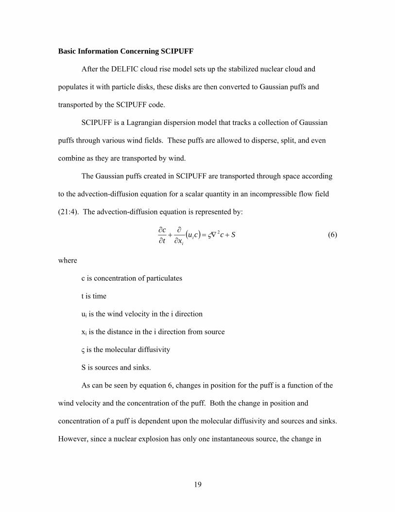
The result of using the glass component of the Heft subsurface distribution as the
particle size distribution in the AFIT smear code for a 1kt surface burst is shown in
Figure 13:
Figure 13: AFIT Smear Code 30 Day Dose Contour for 1kt Surface Burst using Glass
Distribution with 10kph Constant Wind (Units in Roentgen)
Similar to the crystalline distribution, the glass distribution adds very little activity to the
resulting smear from the Heft particle distribution.
The result of using the local particle component of the Heft subsurface
distribution as the particle size distribution in the AFIT smear code with a 1kt surface
burst is shown in Figure 14:
36

Figure 14: AFIT Smear Code 30 Day Dose Rate for 1kt Surface Burst using the Local
Distribution with 10kph Constant Wind (Units in Roentgen)
When compared with the Heft subsurface particle size distribution, the local
particle size distribution is very similar. The AFIT smear code results for both the Heft
tri-component subsurface distribution and the Heft local component subsurface
distribution show a similar shape. However, at similar locations, the smear code results
for the Heft local component show that the contours are approximately twice the value of
the smear code results from the Heft tri-component distribution. This is because the local
component makes up a little less than half, or about 40% of the mass of the Heft tri-
37

component subsurface distribution. Clearly, the local distribution is the driving force for
any significant activity concentrated around ground zero.
0
0.5
1
1.5
2
2.5
3
0 1 2 3 4 5 6
Time [hrs]
g(t)
[1/h
r]
DELFIC
Heft Subsurface
Figure 15: G(t) Comparison for 1kt Surface Burst using Heft Subsurface and DELFIC
Particle Distributions in AFIT Smear Code
Figure 15 shows a g(t) comparison for the Heft subsurface and the DELFIC
subsurface particle distributions. The Heft subsurface distribution clearly has a greater
peak particle deposition than does the DELFIC distribution. As a result it deposits much
more activity in the local area than does the DELFIC distribution. However, starting at
about 30 minutes the DELFIC distribution starts depositing more activity than does the
Heft distribution. Not shown on this graph is that the Heft distribution again deposits
more activity on the ground after 20 hours, which corresponds to 200 km downwind.
38

From this point until the end of the run, the Heft distribution deposits more activity. The
DELFIC distribution deposits its last size bin at about 472 hours while the Heft
subsurface distribution doesn’t deposit its last size bin until 1831 hours. This shows a
significant difference in the amount of small particles between the two distributions.
A Comparison of the DELFIC and Heft Subsurface Particle Distributions for
Varying Yields and Resolutions
As discussed in chapter two, a nuclear weapon surface burst produces a stabilized
cloud. The height of this stabilized cloud as well as its dimensions are dependent upon
several factors including the yield of the nuclear explosion, atmosphere, relative humidity
of the atmosphere and the altitude of the tropopause. In their book The Effects of
Nuclear Weapons, Glasstone and Dolan provide an approximate stabilized cloud height
as a function of the yield of a nuclear device for a surface blast.
Figure 16: Altitudes of the Stabilized Cloud Top and Cloud Bottom Based on Yield for
Surface Bursts (9: 431)
39

For a 1kt surface burst, HPAC 4.03 ran until the last puff was stopped at 12.75
hours. The resulting dose rate contour plot at 12.75 hours is shown in Figure 17.
Figure 17: HPAC 4.03 Dose Rate Contour for 1kt Surface Burst at 12.75 Hours
HPAC 4.04, by comparison, stopped tracking its final puff at 12.25 hours for a 1kt
surface burst. The 4.04 contour plot for a 1kt surface burst at 12.25 hours is shown in
Figure 18.
Figure 18: HPAC 4.04 Dose Rate Contour for 1kt Surface Burst at 12.25 Hours
40

The most noticeable similarity between the two contours is that they both extend
downwind to approximately 120km. However, the 4.03 contour is 30 minutes later than
the 4.04 contour. In those 30 minutes, a small portion of the activity would have decayed
away leaving a smaller total dose rate than is present at the time where the 4.04 contour is
taken from. While both contours extend approximately the same distance downwind, the
4.03 contour shows a larger spread in the north/south direction. This spread is
approximately twice the size of the 4.04 contour. This is apparent in the close up views
of ground zero from 4.03 and 4.04, which are discussed below.
Since the Heft subsurface distribution contains 40% of its mass in the local
distribution, which is made up of large particles with short fall times, it is worth
examining the contours close to ground zero. The dose rate contour at 12 hours for
HPAC 4.03 is shown in Figure 19. Ground Zero is indicated by the yellow dot.
Figure 19: HPAC 4.03 Ground Zero Dose Rate Contour for 1kt Surface Burst at 12
Hours
41

The dose rate increases until it reaches its peak value of 120 rad/hr. For the sake
of readability, the maximum dose rate contour in Figure 19 is 55 rad/hr. However, it is
evident in Figure 19 how sharply the dose rate increases as ground zero is approached.
The dose rate contour at 12 hours for HPAC 4.04 is shown in Figure 20.
Figure 20: HPAC 4.04 Ground Zero Dose Rate Contour for 1kt Surface Burst at 12
Hours
The dose rate increases until it reaches its peak of 55 rad/hr just east of ground
zero. This is a much smaller maximum dose rate at 12 hours than is generated by HPAC
4.03. It should also be noted how much smaller the high dose area is in both the North-
South direction and the East-West direction than the 4.03 contour plot. Not only does the
4.03 contour extend out farther than the 4.04 output, it has a much higher concentration
of radiation close to ground zero than the 4.04 output.
42

Another distinguishing feature is the surge in activity at 20 kilometers east of
ground zero for the 4.04 contour. This surge in activity is a result of the discrete number
of size bins used to model the particle distribution. The 4.03 contour, on the other hand,
appears to decrease monotonically downwind. This feature is confirmed when g(t)
comparisons between the two plots are made.
0
0.2
0.4
0.6
0.8
1
1.2
1.4
1.6
1.8
0 0.5 1 1.5 2 2.5 3 3.5
Time [hrs]
G(t)
[1/h
r]
4
HPAC 4.03
HPAC 4.04
Figure 21: g(t) for 1kt Surface Burst in HPAC 4.03 and 4.04
It should be noted that the g(t) for the HPAC 4.04 run is consistently lower than
the g(t) for HPAC 4.03. This indicates that 4.03 consistently delivers more activity as
activity is integrated transversely to the wind. See Appendix D for details concerning
this calculation.
Due to the sharp dose rate increase close to ground zero, the grounded source
normalization constant was calculated using a series of finer resolutions for both HPAC
43

4.03 and 4.04. A resolution of up to 600 by 600 could be produced by HPAC 4.04,
however, HPAC 4.03 would only produce a resolution of 300 by 300. The results are
shown in Table 3.
Table 3: Comparison of k for 1kt Surface Burst in HPAC 4.03 and 4.04
Resolution HPAC 4.03 HPAC 4.04
100 x 100 3450 1170
200 x 200 3330 1180
300 x300 3460 1190
400 x 400 1190
500 x 500 1210
600 x 600 1210
For a 10kt surface burst, HPAC 4.03 ran until the last puff was stopped at 23 hrs.
The resulting contour is shown in Figure 22.
44

Figure 22: HPAC 4.03 Dose Rate Contour for 10kt Surface Burst at 23 Hours
For a 10kt surface burst, HPAC 4.04 ran until the last puff was stopped at 22hrs.
The resulting contour at 22 hours is shown in.
Figure 23: HPAC 4.04 Dose Rate for 10kt Surface Burst at 22 Hours
45

Many of the features discussed in connection with the set of 1kt bursts are also
present in the set of 10kt bursts. Similar to the 1kt burst set, the 4.03 dose rate contour
for the 10kt burst extends further downwind than does the 4.04 dose rate contour for the
10kt burst. The HPAC 4.03 10kt burst has an grounded source normalization constant of
3020 while the HPAC 4.04 10kt surface burst has a grounded source normalization
constant of 970. These values are much lower than the values of the grounded source
normalization constants found for 1kt blasts. This indicates that as the yield increases,
more activity is lost through dispersion beyond the local area.
For the 100kt run in HPAC 4.03, the run ended when it reached the temporal
domain at 48hrs. The contour plot generated by HPAC 4.03 by the 100kt surface burst is
shown in Figure 24.
Figure 24: HPAC 4.03 Dose Rate Contour for 100kt Surface Burst at 48 Hours
For the 100kt run in HPAC 4.04, the run ended when it reached the temporal
domain of 48hrs.
46

Figure 25: HPAC 4.04 Dose Rate Contour for 100kt Surface Burst at 48 Hours
The difference in the dose rate contours seems to be exaggerated for the 100kt
yield case. For the exact same dose rate time (48 hrs), the DELFIC contour (4.03)
extends out to about 400km while the Heft subsurface contour (4.04) only extends to
approximately 120km. A difference of over 3:1.
The other noticeable feature for the 100kt surface bursts is that the grounded
source normalization constants continue to drop from the values seen with the 1kt surface
bursts. For HPAC 4.03, the grounded source normalization constant for a 100kt surface
burst is 1470 [R-km2/hr-kt], a decrease of 43% from the 1kt grounded source
normalization constant. For HPAC 4.04, the grounded source normalization constant for
a 100kt surface burst is 460 [R-km2/hr-kt], a decrease of 39% from the 1kt grounded
source normalization constant.
47
Variation in the Grounded Source Normalization Constant When Computed from
Different Late Time Dose Rates
The analytical tools used to evaluate the effects of the two distributions under
consideration have used the Way-Wigner formula to find the unit reference dose rate.
The Way-Wigner approximation is a simplification that is used to give a rough
approximation of the radioactive decay of the over 300 radioisotopes that are present
from the time of the explosion to six months after the detonation. The actual decay of the
fission products varies from the t-1.2 law as shown in Figure 26, but Way-Wigner is an
accepted approximation.
It is not possible to compute URDR directly from HPAC. Typically the earliest
possible computation is four hours after burst. Thus it is necessary to use these later dose
rates and adjust them back to one hour using the Way-Wigner formula. However, as
shown in this section, one obtains different results when computing the URDR from
different later modeling times. One reason that HPAC cannot easily compute a direct
URDR is that most of the activity is still in the air at one hour. The URDR is intended to
be used to compute later dose rates (and doses). Therefore, this suspended activity must
be included in the URDR calculation. The computation of airborne activity is a difficult
computation which is not attempted in HPAC, or most other fallout codes.
48

Figure 26: Dose Rate vs. Time (Dashed Line Represents the Way-Wigner
Approximation) (9:392)
For a 100kt explosion in HPAC 4.04, SCIPUFF stops tracking the puffs after
48hrs. The results of the early time decay are evident from examining the decay on the
ground, as shown by the following six figures starting with Figure 27 and ending with
Figure 32. A similar series is shown for HPAC 4.04 starting with Figure 33 and ending
with Figure 38. The red dot on each figure indicates the cloud centerline location for a
constant 10km/hour wind.
49

Figure 27: HPAC 4.03 Dose Rate Contour
for 100kt Surface Burst at 8 Hours
Figure 28: HPAC 4.03 Dose Rate Contour
for 100kt Surface Burst at 16 Hours
Figure 29: HPAC 4.03 Dose Rate Contour
for 100kt Surface Burst at 24 Hours
Figure 30: HPAC 4.03 Dose Rate for 100kt
Surface Burst at 32 Hours
Figure 31: HPAC 4.03 Dose Rate Contour
for 100kt Surface Burst at 40 Hours
Figure 32: HPAC 4.03 Dose Rate Contour
for 100kt Surface Burst at 48 Hours
50

Figure 33: HPAC 4.04 Dose Rate Contour
for 100kt Surface Burst at 8 Hours
Figure 36: HPAC 4.04 Dose Rate Contour
for 100kt Surface Burst at 32 Hours
Figure 34: HPAC 4.04 Dose Rate Contour
for 100kt Surface Burst at 16 Hours
Figure 37: HPAC 4.04 Dose Rate Contour
for 100kt Surface Burst at 40 Hours
Figure 35: HPAC 4.04 Dose Rate Contour
for 100kt Surface Burst at 24 Hours
Figure 38: HPAC 4.04 Dose Rate Contour
for 100kt Surface Burst at 48 Hours
51

In this series of bursts, the dose rate contours grow in the easterly direction (the
direction the wind is blowing to). However, as the fallout contour grows in the easterly
direction with the passing of time, the fallout contour is actually decreasing in the north-
south direction. This is due to the decay of radionuclides.
From these fallout patterns and the grounded source normalization constants in
Table 4, it is once again noticeable how much less activity is deposited on the ground
with HPAC 4.04, which uses the Heft subsurface particle distribution, than with HPAC
4.03, which uses the DELFIC particle distribution. The HPAC 4.03 fallout contour
extend to a much larger maximum east-west distance of 400 km at 24 hours vs. the 300
km distance that the HPAC 4.04 fallout contour extends to in the east-west direction at 24
hours.
Table 4: Grounded Source Normalization Constant vs. Time Comparison for 100kt Blasts
4.03 Hrs 8 16 24 32 40 48
Grounded k 1380 1510 1560 1530 1440 1470
4.04 Hrs 8 16 24 32 40 48
Grounded k 470 500 490 480 470 460
As shown in Table 4, for HPAC 4.03 the maximum value of URDR occurs at 24
hours while the maximum value of the source normalization constant for HPAC 4.04
occurs at 16 hours. The growth of the source normalization constant from 8 hours up
until the maximum value can be attributed to particles falling out of the stabilized cloud.
52

Considering how little activity the crystalline and glass populations add to the local area,
a greater proportion of the activity for the Heft subsurface distribution that makes it to the
ground is found in larger particles than is the case for the DELFIC distribution. This is
because the majority of the activity in the local fallout contours generated by the Heft
subsurface distribution is due to the local fallout lognormal. This means that percentage
wise, a greater proportion of the activity is falling out at an earlier time for the Heft
subsurface distribution than is true for the DELFIC distribution. Because of this, it is
logical that the maximum dose rate for the Heft subsurface distribution would occur at an
earlier time than for the DELFIC distribution, which is observed.
The time when the grounded source normalization constant is at a maximum is
also the time where the center of the stabilized cloud is depositing significant activity to
the outer edge of the 0.01 contour. This is seen in Figure 29 for 4.03 and Figure 34 for
4.04. The stabilized cloud continues to grow with time and the maximum grounded
source normalization constant point is when the smallest particles that add significant
activity are being deposited. After this point, the stabilized nuclear cloud is becoming too
dispersed to add significant fallout to the local area.
The source normalization constant decrease after 24 hours for 4.03 and 16 hours
for 4.04 is less intuitive than the increase up to those times. One possible explanation is
that a proportion of the smaller particles is being resuspended by the constant wind and
therefore being scattered. Smaller particles, which fall out later, would have a greater
probability of resuspension than larger particles. Thus when the source normalization
constant is calculated at later times, these resuspended particles have left the local area
which is being considered. However, to the author’s best knowledge, SCIPUFF does not
53

take resuspension of particles into account. Another possible explanation for this
phenomenon is that when the unit reference dose rate time is calculated using the Way-
Wigner approximation, there is error introduced when some of the activity has decayed
completely away as this lost activity is not corrected back to the unit reference time.
Varying time dose rate contours were also generated for both HPAC 4.03 and
4.04 with 1 kt surface bursts. The results are shown starting in Figure 39 and continuing
through Figure 46.
Similar to the 100kt bursts, the 1kt bursts in the preceding figures show the dose
rate contours grow in the easterly direction (the direction the wind is blowing to) as well
as the decay of short lived radionuclides. The grounded source normalization constants
calculated from the dose rates at various times is reported in Table 5.
Table 5: Grounded Source Normalization Constants for Varying Time 1kt Surface Bursts
4.03 Hrs 4 8 12 12hrs 15min
Grounded k 3080 3650 3580 3460
4.04 Hrs 4 8 12 12hrs 15min
Grounded k 1080 1220 1210 1210
54

Figure 39: HPAC 4.03 Dose Rate Contour
for 1kt Surface Burst at 4 Hours
Figure 40: HPAC 4.03 Dose Rate Contour
for 1kt Surface Burst at 8 Hours
Figure 41: HPAC 4.03 Dose Rate Contour
for 1kt Surface Burst at 12 Hours
Figure 42: HPAC 4.03 Dose Rate Contour
for 1kt Surface Burst at 12.75 Hours
55

Figure 43: HPAC 4.04 Dose Rate Contour
for 1kt Surface Burst at 4 Hours
Figure 45: HPAC 4.04 Dose Rate Contour
for 1kt Surface Burst at 12 Hours
Figure 44: HPAC 4.04 Dose Rate Contour
for 1kt Surface Burst at 8 Hours
Figure 46: HPAC 4.04 Dose Rate Contour
for 1kt Surface Burst at 12.25 Hours
56

In both HPAC 4.03 and 4.04, the highest grounded source normalization constant
occurs at eight hours. This is an indication that most of the activity has fallen from the
stabilized cloud to the ground at the eight hour point for both HPAC 4.03 and 4.04.
Whereas the 100kt bursts showed a different time for max k with an eight hour time
interval, the one kt bursts do not show a difference with a four hour time step. The lower
stabilization altitude of the nuclear cloud may help to account for this since the shorter
fall distance for the particles will compress the fall time differences that different particle
sizes exhibit. While the highest grounded source normalization constant does occur at 8
hours, it should be noted that there is little difference between the eight hour grounded
source normalization constants and the grounded source normalization constants for 12
hours and later since the shorter time steps help to minimize the effects of decay.
57

V. Interaction of Particle Size Distribution with Other Variable Parameters in
HPAC
This section looks at how the particle size distributions in HPAC 4.03 and 4.04
interact with other parameters in HPAC. Specific consideration is given to the effects of
varying surfaces, rain scavenging and varying constant winds.
Effects of Varying Surfaces
In SCIPUFF differing surfaces such as vegetative canopies are affected by dry
deposition processes and so the type of surface over which the fallout cloud is traveling
helps to determine the mass flux of particles at the surface or how fast the fallout is
deposited onto the ground. The roughness of the surface can also result in self-shielding
by the ground of the radiation reaching the one meter high detector.
The default surface in HPAC 4.03 is the cultivated surface. This surface has a
relatively high canopy height as well as a relatively low bowen ratio and albedo (See
Table C-1 in Appendix C). The low bowen ratio indicates that cultivated is a fairly moist
surface. The low albedo means that it absorbs most of the radiation from the sun that is
incident upon it.
When a 1kt blast was run in HPAC 4.03, the last puff was tracked until 12.75
hours. The grounded source normalization constant for this run is 3460 [R-km2/hr-kt].
For HPAC 4.04, the last puff was tracked until 12.25 hours with a grounded source
normalization constant of 1210 [R-km2/hr-kt]. The resulting contour plots for a
cultivated surface at 12 hours are shown in Figure 47 and Figure 48.
58

Figure 47: HPAC 4.03 Dose Rate Contour for 1kt Surface Burst with Cultivated Surface
at 12 Hours
Figure 48: HPAC 4.04 Dose Rate Contour for 1kt Surface Burst with Cultivated Surface
at 12 Hours
The forest surface has the highest canopy of all the surfaces at 10m. It also has a
relatively high Bowen ratio and low Albedo. In HPAC 4.03, the last puff was tracked
until 11.5 hours. In HPAC 4.04, the last puff was tracked until 11.0 hours. This is the
59

shortest run time for any of the surfaces as would be expected since forest has the largest
canopy. The large canopy of forest means there is more friction induced effects, such as
eddies, over that surface as compared to the other surfaces. This results in the fallout
particles traveling slower over this surface and thus being more likely to be deposited per
unit area. The grounded source normalization constant for a forest surface in HPAC 4.03
is 3720 [R-km2/hr-kt] while in HPAC 4.04 it is 1240 [R-km2/hr-kt]. This is the highest
grounded source normalization constant for any surface in both 4.03 and 4.04. This
would seem to indicate that radiation shielding as a result of the surface isn’t being taken
into account in the HPAC dose rate calculations. The contour plots at 12 hours for a 1kt
surface burst with a forest surface for both 4.03 and 4.04 is shown in Figure 49 and
Figure 50. As seen in Figure 49 and Figure 50 the areas of the 0.001 fallout contour is
larger for both the HPAC 4.03 and 4.04 1kt forest runs when compared to their HPAC
4.03 and 4.04 cultivated surface counterparts in Figure 47 and Figure 48 respectively.
This is because of the increased activity deposition on the ground due to the forest
surface in comparison to the cultivated surface.
The urban surface has a canopy height that is smaller than either the forest
surface or the cultivated surface, but it is larger than the water, desert and grassland
surfaces. As such, in HPAC 4.03 the time that its last puff was tracked until was longer
than either forest or cultivated, but shorter than grassland, desert and water. In HPAC
4.03, the last puff was tracked until 13.25 hours. However, in HPAC 4.04, the last puff
was tracked until 11.5 hours, which is the same amount of time that the forest surface was
tracked until and less time than the puff was tracked over the cultivated surface.
60

Figure 49: HPAC 4.03 Dose Rate Contour for 1kt Surface Burst with Forest Surface at
12 Hours
Figure 50: HPAC 4.04 Dose Rate Contour for 1kt Surface Burst with Forest Surface at
12 Hours
One possible explanation for this is that the deposition velocity is increased by having not
only a high canopy, but also a much higher bowen ratio than either the forest surface or
the cultivated surface has. This higher bowen ratio affects the smaller particles by
increasing their deposition velocity. Since the Heft distribution has a greater amount of
these smaller particles than does the DELFIC distribution, HPAC 4.04 tracked the last
61

puff over the urban surface than it did the last puff over the cultivated surface. The
grounded source normalization constant for HPAC 4.03 Urban run is 2730 [R-km2/hr-kt]
while for the HPAC 4.04 run it is 1330 [R-km2/hr-kt].
Figure 51: HPAC 4.03 Dose Rate Contour for 1kt Surface Burst with Urban Suface at 12
Hours
Figure 52: HPAC 4.04 Dose Rate Contour for 1kt Surface Burst with Urban Surface at
12 Hours
62

The grassland surface has a relatively small canopy at only 0.25 meters, but it is a
much higher canopy than either desert or water. For the HPAC 4.03 run the last puff was
tracked until 14.0 hours. For the HPAC 4.04 run the last puff was tracked until 12.25
hours. This follows the general trend of a lower canopy having a slower deposition
velocity. The grounded source normalization constant for 4.03 grassland is 3310 [R-
km2/hr-kt] while for 4.04 it is 1240 [R-km2/hr-kt].
Figure 53: HPAC 4.03 Dose Rate Contour for 1kt Surface Burst with Grassland Surface
at 12 Hours
Figure 54: HPAC 4.04 Dose Rate Contour for 1kt Surface Burst with Grassland Surface
at 12 Hours
63
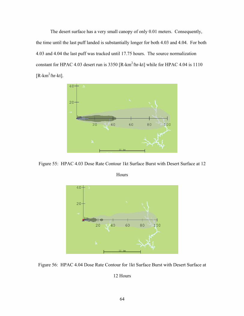
The desert surface has a very small canopy of only 0.01 meters. Consequently,
the time until the last puff landed is substantially longer for both 4.03 and 4.04. For both
4.03 and 4.04 the last puff was tracked until 17.75 hours. The source normalization
constant for HPAC 4.03 desert run is 3350 [R-km2/hr-kt] while for HPAC 4.04 is 1110
[R-km2/hr-kt].
Figure 55: HPAC 4.03 Dose Rate Contour 1kt Surface Burst with Desert Surface at 12
Hours
Figure 56: HPAC 4.04 Dose Rate Contour for 1kt Surface Burst with Desert Surface at
12 Hours
64

Water is a very smooth surface with no canopy. Therefore, like the desert
surface, it will track puffs for a long time in comparison with the other surfaces. For
HPAC 4.03, the last puff was tracked until 16.5 hours while for HPAC 4.04 the last puff
was tracked until 16.25 hours. The grounded source normalization constant for the
HPAC 4.03 water surface is 3230 [R-km2/hr-kt] while for HPAC 4.04 it is 1150 [R-
km2/hr-kt].
Figure 57: HPAC 4.03 Dose Rate Contour for 1kt Surface Burst with Water Surface at
12 Hours
Figure 58: HPAC 4.04 Dose Rate Contour for 1kt Surface Burst with Water Surface at
12 Hours
65
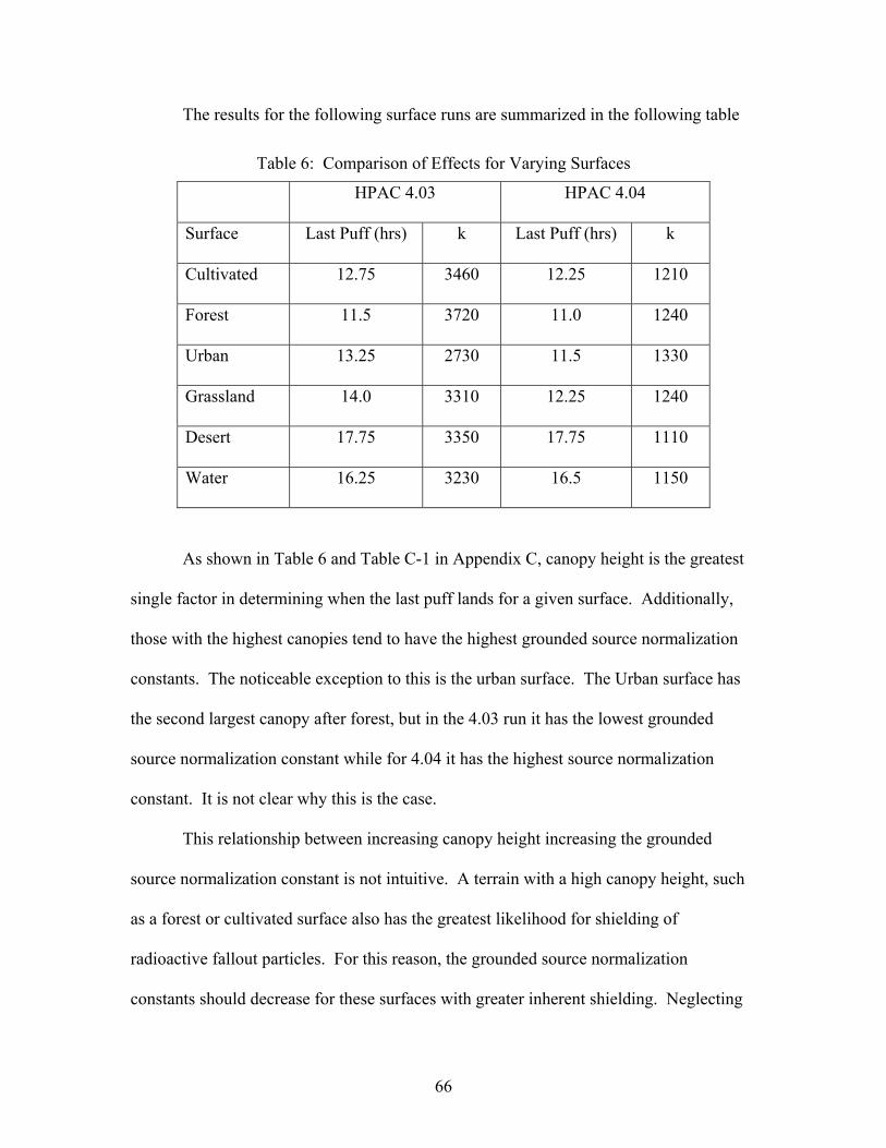
The results for the following surface runs are summarized in the following table
Table 6: Comparison of Effects for Varying Surfaces
HPAC 4.03 HPAC 4.04
Surface Last Puff (hrs) k Last Puff (hrs) k
Cultivated 12.75 3460 12.25 1210
Forest 11.5 3720 11.0 1240
Urban 13.25 2730 11.5 1330
Grassland 14.0 3310 12.25 1240
Desert 17.75 3350 17.75 1110
Water 16.25 3230 16.5 1150
As shown in Table 6 and Table C-1 in Appendix C, canopy height is the greatest
single factor in determining when the last puff lands for a given surface. Additionally,
those with the highest canopies tend to have the highest grounded source normalization
constants. The noticeable exception to this is the urban surface. The Urban surface has
the second largest canopy after forest, but in the 4.03 run it has the lowest grounded
source normalization constant while for 4.04 it has the highest source normalization
constant. It is not clear why this is the case.
This relationship between increasing canopy height increasing the grounded
source normalization constant is not intuitive. A terrain with a high canopy height, such
as a forest or cultivated surface also has the greatest likelihood for shielding of
radioactive fallout particles. For this reason, the grounded source normalization
constants should decrease for these surfaces with greater inherent shielding. Neglecting
66

the effects of washout in water, one would expect desert and water to show the highest
grounded source normalization constants instead of the lowest.
Effects of Rain Out
Precipitation scavenging by rain is a major removal mechanism for aerosols
(particles ranging from 10-4 µm to tens of micrometers). Precipitation scavenging
accounts for the removal of approximately 80-90% of the mass of aerosols in the
atmosphere. Most of the remaining aerosol mass is removed through gravitational
settling (23:153-154). Larger aerosol particles, aerosol particles greater than 1 µm, are
collected more efficiently than smaller ones since the smaller aerosols will follow the
streamlines around the raindrop instead of being impacted by the collecting raindrop
(23:174).
If a fallout cloud encounters precipitation, a large portion of that cloud could be
brought down by the precipitation (8:416). Based on the results of the AFIT smear code,
all of the crystalline particles in the Heft subsurface distribution are dispersed into the
atmosphere and a good portion of the glass distribution as well. One would expect a
significant increase in the activity on the ground when there is precipitation present.
Fallout close to ground zero that is due to larger particles should not be greatly
influenced by precipitation scavenging. This is because precipitation scavenging will not
significantly affect the larger particles that fallout quickly by ground zero. However,
downwind precipitation scavenging should cause surface deposition of smaller particles
that would otherwise totally escape the local area.
Another consideration that should be accounted for is the yield of the blast.
Typically rain clouds can be found between 10,000 to 30,000 feet (9:416). Generally
67

speaking, lighter rain clouds are found at the lower end of the altitude range while heavy
rain clouds are at the higher end of the altitude range. Since that altitude that the nuclear
cloud stabilizes at depends upon the yield of the burst, scavenging has less effect on high
yield weapons. At 10kt the top of the stabilized cloud is usually about 19 kft while the
bottom of the cloud is usually about 10 kft. At this yield, the entire stabilized cloud will
usually be encompassed by the rain cloud or be completely below the rain cloud. At
100kt the top of the stabilized nuclear cloud is at about 40,000 feet while the bottom is at
about 20,000 feet. This would mean that for a light rain there would be little to no
scavenging of a 100kt burst, however, for a heavy rain, there would most likely be at
least some scavenging. For nuclear explosives with yield greater than 100kt, scavenging
will have little effect on the source normalization constant itself but might rearrange
where the fallout lands.
A good historical example of the effect of precipitation scavenging causing fallout
activity on the ground is the precipitation scavenging that occurred after the airburst shot
associated with the bombing of Nagasaki. An airburst is not expected to result in any
appreciable local fallout, however, after the Nagasaki airburst, there were some torrential
rains. Measurements were made after the bombing and appreciable fallout was found on
the ground. Krieser (13:15) assumes that 100% of activity should be scavenged in a rain
storm. McGahan assumes that scavenging is 100% for particles with fall velocities less
than the velocity of the rain itself (15:4).
SCIPUFF, which is the transport model used by HPAC, accounts for precipitation
washout by adding a new sink term that must be accounted for in SCIPUFF’s
68

69
conservation of mass. This new factor further modifies the conservation of mass
equation to
( )Rs FFdtdQ
+−= (17)
where
FBR B is the mass flux due to rain out (21:56). FBR B is defined by the following
equation:
R
RQFτ
= (18)
where
t BR B is the washout time scale.
The washout time scale is the inverse of the scavenging coefficient, wBs B. The
scavenging coefficient is defined by
( )rpr
os DDE
Dp ,3/2
=ω (19)
where
pBo B is the precipitation rate in mmhP
-1P,
DBrB is the raindrop diameter (an assumed range) in microns,
E is the collision efficiency,
DBp B is the particle diameter in microns (21:57).
The precipitation rate, pBoB, is assumed to be 0.5 mmh P
-1P for a light rain, 10 mmhP
-1P
for a moderate rain and 25 mmhP
-1Pfor a heavy rain (21:59-60). These are settings that the
user can specify within HPAC.
The Marshall Palmer raindrop distribution is assumed so that

70
rDr eN ε−= 08.0 (20)
where ε=41(pBo B)P
-21P (21:57).
The average raindrop diameter is then assumed to be
ε3
=rD (21)
The collision efficiency is a function of the raindrop diameter, the Reynold’s
number, the Stokes number and the Schmidt number (21:57-58).
Sykes et al suggest that the model overestimates washout and as such they
multiply the scavenging coefficient by 1/3. The authors of the SCIPUFF Technical
Documentation offer the following to illustrate how the SCIPUFF rain scavenging agrees
with the rain scavenging model proposed by Neito et al.

Th
lines deno
A
surface bu
10−8
10−6
10−4
10−2
100
10−3 10−1 10+1
ωs(s−1)
Dp (µm)
Heavy rain
Drizzle
Figure 59: Scavenging Coefficient vs. Particle Diameter [From Sykes etal 59]
71
e solid lines in Figure 59 denote the model described above and the dashed
te the model of Nieto et al.
series of HPAC runs was conducted for both light rain and heavy rain for a 1kt
rst for both 4.03 and 4.04. The results are shown from Figure 64 to Figure 65:

Figure 63: HPAC 4.04 Dose Rate
Contour for 1kt Surface Burst with No
Rain at 12 Hours
Figure 60: HPAC 4.03 Dose Rate
Contour for 1kt Surface Burst with No
Rain
Figure 61: HPAC 4.03 Dose Rate
Contour for 1kt Surface Burst with Light
Rain at 12 Hours
Figure 64: HPAC 4.04 Dose Rate
Contour for 1kt Surface Burst with Light
Rain at 12 Hours
Figure 65: HPAC 4.04 Dose Rate
Contour for 1kt Surface Burst with
Heavy Rain at 12 Hours
Figure 62: HPAC 4.03 Dose Rate
Contour 1kt Surface Burst with Heavy
Rain at 12 Hours
72
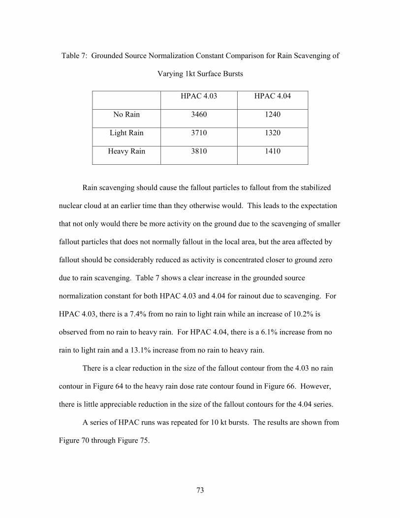
Table 7: Grounded Source Normalization Constant Comparison for Rain Scavenging of
Varying 1kt Surface Bursts
HPAC 4.03 HPAC 4.04
No Rain 3460 1240
Light Rain 3710 1320
Heavy Rain 3810 1410
Rain scavenging should cause the fallout particles to fallout from the stabilized
nuclear cloud at an earlier time than they otherwise would. This leads to the expectation
that not only would there be more activity on the ground due to the scavenging of smaller
fallout particles that does not normally fallout in the local area, but the area affected by
fallout should be considerably reduced as activity is concentrated closer to ground zero
due to rain scavenging. Table 7 shows a clear increase in the grounded source
normalization constant for both HPAC 4.03 and 4.04 for rainout due to scavenging. For
HPAC 4.03, there is a 7.4% from no rain to light rain while an increase of 10.2% is
observed from no rain to heavy rain. For HPAC 4.04, there is a 6.1% increase from no
rain to light rain and a 13.1% increase from no rain to heavy rain.
There is a clear reduction in the size of the fallout contour from the 4.03 no rain
contour in Figure 64 to the heavy rain dose rate contour found in Figure 66. However,
there is little appreciable reduction in the size of the fallout contours for the 4.04 series.
A series of HPAC runs was repeated for 10 kt bursts. The results are shown from
Figure 70 through Figure 75.
73
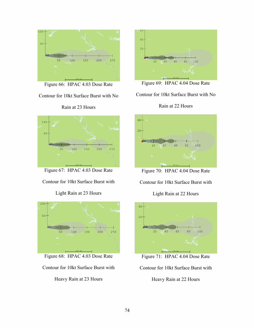
Figure 69: HPAC 4.04 Dose Rate
Contour for 10kt Surface Burst with No
Rain at 22 Hours
Figure 66: HPAC 4.03 Dose Rate
Contour for 10kt Surface Burst with No
Rain at 23 Hours
Figure 70: HPAC 4.04 Dose Rate
Contour for 10kt Surface Burst with
Light Rain at 22 Hours
Figure 67: HPAC 4.03 Dose Rate
Contour for 10kt Surface Burst with
Light Rain at 23 Hours
Figure 68: HPAC 4.03 Dose Rate
Contour for 10kt Surface Burst with
Heavy Rain at 23 Hours
Figure 71: HPAC 4.04 Dose Rate
Contour for 10kt Surface Burst with
Heavy Rain at 22 Hours
74

From a visual standpoint there is very little difference in the 10 kt blast with no
rain, light rain and heavy rain.
Table 8: Grounded Source Normalization Constant for 10kt Surface Burst with Varying
Levels of Rain
HPAC 4.03 HPAC 4.04
No Rain 3030 970
Light Rain 3050 990
Heavy Rain 3090 1000
Table 8 shows very little difference in activity deposition on the ground due to
rainout for a 10kt surface burst. The difference from no rain to heavy rain is only 2% for
4.03 while for 4.04 the difference is only 3.4%. Visually there is some difference in the
sizes of the dose rate contour for the 4.03 sequence, but again, there is no noticeable
difference in the 4.04 10kt series.
While HPAC shows that the rain is a scavenging activity, it is not scavenging
enough activity to be a realistic representation of the effect rainout would have on the
airborne fallout that doesn’t normally fall to the local area. Based on historical examples
of washout, it is not unreasonable to assume that a heavy rain would effectively scavenge
all of the activity in a fallout cloud. It is evident that the true source normalization
constant must be at least 3800 [R-km2/hr-kt] since this is the source normalization
constant that is achieved from an HPAC 4.03 1kt surface burst with heavy rain. The
AFIT smear code indicates that in the Heft subsurface particle distribution, that neither
75

the crystalline nor the glass particles contribute significant activity to the local fallout
area. If it is assumed that none of the crystalline population, which makes up 17% of the
mass, falls in the local area and that the crystalline population makes up 17% of the
activity, then there is at lest 17% of the true activity that should be deposited in the local
area due to rain scavenging. 17% of 3800 gives an increase of 650 in the HPAC 4.04
source normalization constant from no rain to heavy rain. However, there is an increase
of merely 160 [R-km2/hr-kt] for the 1kt surface burst and only 30 [R-km2/hr-kt] for the
10kt surface burst, even though the stabilized clouds for both yields would most likely be
within a rain cloud. The author cannot explain this anomaly.
Effects of Different Constant Wind Speeds for DELFIC and Heft Three Component
Particle Distributions
As discussed earlier, SCIPUFF tracks a Gaussian puff of particle through the
advection-diffusion equation (Equation 19). Wind velocity not only moves the puff, but
also affects the concentration of puffs. The stronger the wind that acts upon an individual
puff, the more diffusion and the lower the concentration that puff will have over time.
A series of runs was accomplished using both HPAC 4.03 and 4.04 using a
constant wind of 5kph, 10kph and 15kph. The results for HPAC 4.03 are shown from
Figure 72 through Figure 74. The results for HPAC 4.04 are shown from Figure 75
through Figure 77.
76

Figure 72: HPAC 4.03 Dose Rate Contour for 1kt Surface Blast with 5kph Constant Wind
Figure 73: HPAC 4.03 Dose Rate Contour for 1kt Surface Burst with 10kph Constant Wind
Figure 74: HPAC 4.03 Dose Rate Contour for 1kt Surface Burst with 15kph Constant Wind
77

Figure 75: HPAC 4.04 Dose Rate Contour for 1kt Surface Burst with 5kph Constant Wind
Figure 76: HPAC 4.04 Dose Rate Contour for 1kt Surface Burst with 10kph Constant Wind
Figure 77: HPAC 4.04 Dose Rate Contour for 1kt Surface Burst with 15kph Constant Wind
78

As can be seen, the slower the wind, the less the fallout cloud is dispersed and the
more activity falls to the ground in amounts significant enough to be counted. As the
wind increases, the fallout smear increases in the east-west direction, but drastically
decreases in the north-south direction.
Table 9: Grounded Source Normalization Constant Summary for 1kt Surface Bursts with
Different Winds
Wind Speed (kph) HPAC 4.03 HPAC 4.04
5 (Dose Rate taken
at 12 hrs)
3510 1310
10 3460 1210
15 3380 1160
Table 9 shows the summarization of grounded source normalization constant for
Different Winds. There is a trend that the less wind, the higher the grounded source
normalization constant. If the wind acts to diffuse the stabilized nuclear cloud, then
slower wind allows more of the activity to be deposited in the local area. While there is a
definite trend for increasing grounded source normalization constant with decreasing
wind, it should be noted that the differences are not major.
Figure 78 and Figure 79 show g(t) for differing winds for HPAC 4.03 and 4.03
respectively.
The noticeable feature of Figure 78 and Figure 79 is that g(t) doesn’t vary much
with different wind speeds. This indicates that gravitational settling is the major
79

deposition mechanism and that the diffusion of the stabilized nuclear cloud is not a major
concern for total activity deposition.
0
0.2
0.4
0.6
0.8
1
1.2
1.4
0 2 4 6 8 10 12
Time [hrs]
G(t)
[1/h
r]
5kph10kph15kph
Figure 78: G(t) Comparison for HPAC 4.03 1kt Surface Burst with Different Winds
0
0.1
0.2
0.3
0.4
0.5
0.6
0 2 4 6 8 10 12
Time [hours]
G(t)
[1/h
r] 5kph10kph15kph
Figure 79: G(t) Comparison for HPAC 4.04 1kt Surface Burst with Different Winds
80

VI. Research Summary and Conclusions This final chapter provides a summation of and conclusions drawn from the
preceding research. Recommendations for further research on related topics are also
included.
Research Summary
This research compared the DELFIC and Heft subsurface particle distributions for
nuclear fallout modeling in HPAC. Since the Heft subsurface particle distribution is
created from a low yield test shot in the Nevada desert, it is important to understand the
implications of using this distribution as the sole distribution in HPAC for all surface
burst fallout modeling. Through a series of HPAC runs using visual analysis, grounded
source normalization constant and the rate of arrival function g(t), the variation in HPAC
output was analyzed for varying yields, varying times, varying surfaces, rainout and
different wind speeds.
Conclusions
HPAC 4.04, which uses the Heft subsurface distribution, consistently deposits
about a third of the activity in the local area as compared to HPAC 4.03, which uses the
DELFIC particle distribution. Based on the CASTLE BRAVO test, the expected source
normalization constant should be between 2590 and 3880 [R-km2/hr-kt] (8:494). It
should be noted that CASTLE BRAVO was a 15 Megaton shot (9:63). Some of Castle
Bravo’s fallout penetrated the tropopause and did not contribute to local fallout. Thus,
the amount of fallout in the local area would be much less per kiloton of yield than for
lower yield bursts, which have no global component. The highest source normalization
constant generated was about 3720 [R-km2/hr-kt] for a 1kt burst with forest surface in
81

HPAC 4.03. This is well within the expected source normalization constant based on
CASTLE BRAVO. The highest source normalization constant generated by HPAC 4.04
is 1240 [R-km2/hr-kt] and this also was for a 1kt surface burst with the forest surface.
This value is far lower than that expected based on the CASTLE BRAVO source
normalization constant.
When varying the yield of the nuclear detonation two things stand out. The first
is that the grounded source normalization constant drops dramatically with increasing
yield. In HPAC 4.03 it drops from 3460 to 1470 [R-km2/hr-kt] and a similar drop is seen
in HPAC 4.04 from 1210 to 458 [R-km2/hr-kt]. These grounded source normalization
constants are very low and seem to indicate that the fallout activity is being
underestimated at higher yields or more of it is escaping the local area. The second
noticeable feature is the area affected by fallout for varying yields. For 1kt, the HPAC
4.03 0.01 rad/hr dose rate contour extends a little less than twice the downwind distance
that the HPAC 4.04 0.01 rad/hr dose rate contour extends. However, for 100kt, the
HPAC 4.03 0.01 rad/hr dose rate contour extends more than three times the downwind
distance that the HPAC 4.04 0.01 rad/hr dose rate contour extends. This indicates that
either HPAC 4.03 is vastly overestimating the area affected by fallout for high yield
weapons, or HPAC 4.04 is grossly underestimating that area.
The effects of varying times on the grounded source normalization constant
showed that HPAC 4.04 stops adding significant activity to the local area at a much
sooner time than does HPAC 4.03. This can also be inferred from the difference in area
affected by fallout between HPAC 4.03 and 4.04.
82

Varying surfaces in HPAC produced differing concentrations of fallout. In
general, the higher the canopy height, the greater the deposition rate of fallout particles is.
While the varying surfaces do appear to affect the deposition rate of fallout, there is no
indication that differing surface roughness factors are taken into consideration amongst
the various surfaces. Surface roughness factors should pose a large contribution to the
grounded source normalization constants seen from fallout modeling. This issue should
be addressed in HPAC.
Rainout is an efficient scavenging mechanism for particles greater than 1 micron
in diameter. Since the Heft distribution places a considerable portion of its mass in the
fine crystalline distribution with a mass median diameter of 6.8 microns, rainout should
greatly increase the grounded source normalization constant observed from HPAC 4.04
and greatly decrease the fallout area seen by both HPAC 4.03 and 4.04. However, the
series of 1kt and 10kt rain runs showed only a slight increase in the grounded source
normalization constant for both HPAC 4.03 and 4.04. Additionally, there was little
difference in the area affected by fallout from surface bursts without rain and surface
bursts with rain.
The effects of different constant winds on HPAC 4.03 and 4.04 is primarily to
change the area affected by fallout. The function g(t) is not greatly influenced by
different constant winds for either HPAC 4.03 or 4.04. This indicates that gravitational
settling is the dominant mechanism for particle deposition in HPAC.
Recommendations for Future Research
This thesis leads to four recommendations for future research.
83

First, the Heft subsurface distribution should be benchmarked against historic test
data for both high yield bursts and bursts over differing soils. The Heft subsurface
distribution should be benchmarked against both the DELFIC distribution and the Heft
two-component surface distribution for Pacific test shots. The research should seek to
answer the question of which distribution is most appropriate for high yields, silicate soil
and coral soil.
Second, the effects of rain scavenging in SCIPUFF should be investigated more
thoroughly. A validation of rain scavenging of airburst and crystalline fallout particles by
SCIPUFF could be accomplished by benchmarking SCIPUFF particle deposition against
the historical example of rainout seen at Nagasaki.
Third, the activity distribution used with the Heft subsurface distribution should
be analyzed. Heft’s activity distribution could be modeled for each equal mass size class
by integrating both the refractory and volatile distributions for each size group to find the
percent of volatile and refractory in each size group. After this, the Freiling ratio for each
mass chain could be determined. Knowing the cumulative yield and the Freiling ratio for
each mass chain, the number of volatiles in a particular mass chain could then be
apportioned for a given equal mass size group based on the percentage of volatiles and
refractories in that equal mass size group determined by the Heft subsurface refractory
and volatile distributions. The results of fallout based on the Heft subsurface activity
distribution could then be compared with the current activity distribution by
benchmarking against historic test shots.
Fourth, the SCIPUFF transport code should be benchmarked against a classic disk
tosser routine (such as DELFIC) for fallout modeling. SCIPUFF may globally disperse
84
more of the activity from a nuclear detonation than a disk tosser and for this reason this
research should focus on the difference in both the amount of activity deposited by each
transport code and the area affected by fallout by benchmarking both transport codes
against historic test shots.
Fifth, comparison should be made between a traditional fallout model such as
HPAC that transports fallout based on current weather conditions and predictions and an
inline weather fallout model that considers the effects a nuclear burst has on the weather
and then transports fallout particles based on the updated weather predictions.
Sixth, SCIPUFF should be examined to track the puffs as a function of time and
space, both vertically and horizontally. In this way, activity could be integrated vertically
in order to determine how much activity is still in the air as a function of time after
detonation. This activity should be tracked until it is grounded. By doing this integration
immediately after detonation, the source normalization constant for HPAC could be
determined. Then by tracking the activity until it lands and integrating the activity over
all ground, a determination could be made of whether or not HPAC conserves activity.
85

86
Glossary
A - Area
A(d) - the activity distribution as a function of fallout particle diameter
a Bi B - the number of atoms of isotope i in a sample
c – concentration of puff
c BDB – coefficient of drag
GdD - Dose Rate on the ground at the unit time.
rD - average raindrop diameter
d – diameter of fallout particle
DELFIC – Defense Land Fallout Interpretative Code
FBTB - the total number of equivalent fissions in all size classes
FBi B - the total number of equivalent fissions in the iP
thP size class
FBp B - the drag force
FBR B - mass flux due to rain out
fBi B - the number of fissions needed to create the number of radioisotopes observed
in the fallout particle
k – grounded source normalization constant [R-kmP
2P/hr-kt]
kt - Kiloton
M - the mass of the puff
mBk B– mass fraction of the k P
thP size group
N(d) –the number of particles of diameter d
Q – total mass of all puffs

87
RBi B - the fration of fissions in the iP
thP mass chain that obeys radial distribution
r Bi,j B - the ratio of the number of fissions needed to create the number of radioisotopes
observed for isotope i to the number of fissions needed to create the number of
radioisotopes observed for isotope j.
r BpB - the equivalent spherical particle radius
SBi B - the fraction of fissions in the iP
thP mass chain that appears with constant specific
Activity
S – Sources and Sinks
t - time
u Bi B - the wind velocity in the i direction
URDR – Unit-Time Reference Dose Rate
vBDB - downward velocity of particles
vBg B- particle fall speed due to gravity
W - weapon yield in kilotons
xBcB, yBcB, z BcB - the location of the Gaussian puff centroid
YBi B - the cumulative fission yield of isotope i in mass chain m
z BGZB - the altitude of ground zero
z BHOB B - the altitude of the height of burst above ground zero
β - the natural logarithm of the standard deviation
α B0B - the natural logarithm of the median diameter in microns
l - the radioactive decay constant
ξ - the direction transverse to the constant wind
r BaB - air density

88
r BpB - particle material density
ς - molecular diffusivity
σ BhB - the standard deviation of a Gaussian puff in the horizontal axis
σ Bi B - the standard deviation of the logB10B(diameter) for the ith population
σ BzB - the standard deviation of a Gaussian puff in the vertical axis
t BR B - washout time scale
iφ - the percentage of mass for the ith population
ix - the logB10 B of the average diameter in microns for the ith population
χ - the logB10 B of the diameter in microns
ψ Bi B - the slope of the Freiling plot for isotope i
ω Bs B – washout timescale
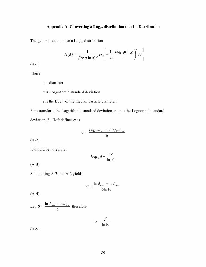
89
Appendix A: Converting a LogB10 B distribution to a Ln Distribution The general equation for a LogB10B distribution
( )⎥⎥⎦
⎤
⎢⎢⎣
⎡⎟⎠⎞
⎜⎝⎛ −
−= dddLog
ddN
210
21exp
10ln21
σχ
σπ
(A-1) where d is diameter σ is Logarithmic standard deviation χ is the LogB10 B of the median particle diameter. First transform the Logarithmic standard deviation, σ, into the Lognormal standard deviation, β. Heft defines σ as
6
min10max10 dLogdLog −=σ
(A-2) It should be noted that
10ln
ln10
ddLog =
(A-3) Substituting A-3 into A-2 yields
10ln6lnln minmax dd −
=σ
(A-4)
Let 6
lnln minmax dd −=β therefore
10lnβσ =
(A-5)

90
Next we transform the exponential from LogB10 B to ln
ββσ
5.0
5.0
5.01010 lnln
10ln
10lnln
10lnln
dddd
dLogdLog −=
−=
−
(A-6) Finally, combining all these things together
( )⎥⎥⎦
⎤
⎢⎢⎣
⎡⎟⎟⎠
⎞⎜⎜⎝
⎛ −−=
25.0lnln
21exp
10ln10ln
2
1ββπ
dddN
which equals
⎥⎥⎦
⎤
⎢⎢⎣
⎡⎟⎟⎠
⎞⎜⎜⎝
⎛ −− dddd
25.0lnln
21exp
21
ββπ
(A-7)

91
Appendix B: Summarization of Freiling Ratios and Heft Distributions\
Fission produces over 300 different types of fission fragments that go through a
series of β/γ decays until they reach stable isotopes. The series of atoms formed through
the fission fragments decay are known as mass chains. Freiling ratios help to
characterize these mass chains in terms of how volatile or refractory they are as a whole.
Freiling ratios are based on the results of radiochemical analysis of fallout
particles. Both the total number of atoms and the number of atoms of each radioisotope
are counted in each fallout particle. The first long lived radioisotope of a given mass
chain is chosen to represent the mass chain.
The number of fissions needed to create the number of radioisotopes observed in
the fallout particle is:
fBi B= aBi B/YBi B (B-1)
where
aBi B is the number of atoms of isotope i in a sample
YBi B is the cumulative fission yield of isotope i in mass chain m (7:1994).
A purely volatile isotope, P
89PSr, is used to reference against other isotopes. A ratio
of any isotope is then set up against P
89PSr (7:1995):
89
89, ff
r ii = . (B-2)
If the fallout particle had all of the fission-fragment isotopes in the same ratios as
what can be expected from fission, then rBi,89 B would equal one. If the isotope i were
distributed in the same proportion as P
89PSr in the fallout particle, then isotope i would be

92
volatile. However, because fractionation alters the isotope proportions, this will not be
the case.
Freiling chose P
95PZr to represent a purely refractory isotope. This leads to a
refractory to volatile ratio (7:1994)
89
9589,95 f
fr = . (B-3)
For each isotope of interest (and by extension each mass chain of interest), r Bi,89B
and rB95,89B are determined for each fallout particle size group. r Bi,89B is then plotted on the
ordinate and r B95,89B is plotted on the abscissa for each mass chain of interest. A straight
line is then fit to the data. The slope of this line determines the classification of the mass
chain. Mass chains with Freiling ratio slopes between 0.98 and 1.0 are considered
refractory. If the slope is between 0.0 and 0.02, the mass chain is considered to be purely
volatile and slopes between 0.02 and 0.98 are considered mixed chains (6:6).
Heft Characterization of Radioactive Particles from Nuclear Tests
In his article “The Characterization of Radioactive Particles from Nuclear
Weapons Tests”, Heft analyzed samples taken from stabilized clouds following nuclear
explosions. Heft proposed a series of logarithmic distributions to fit the particle sizes that
he observed from differing types of nuclear bursts. He created different particle
distributions for airburst detonations, Coral Island surface bursts and cratering
detonations. I will briefly consider Heft’s Coral Island surface distributions and then
focus on his cratering detonation distributions.
Heft asserts that for land surface bursts the particle population divides into two
distinct components, which Heft referred to as crystalline and glass particles. The

crystalline particles are made up of soil material which entered the fireball at a later time
and hence were never melted. Because these particles arrived at a later time, the activity
associated with them is exclusively surface distributed volatiles. Since the crystalline
particles are soil material that has surface deposition of radionuclides from the bomb
debris, the density of the crystalline particles is identical to that of the soil material.
Heft defines the glass population as soil material which entered the fireball at a
time earlier to the crystalline material. As a result the glass particles were at least
partially melted. In addition, the amount of soil material that would be considered glass
particles is much greater than the amount of soil material that would result in crystalline
particles. As a result of increased material and time in the fireball, the mean diameter of
a glass particle is larger than the mean diameter of a crystalline particle. Also, since glass
particles are local soil material that is partially or fully melted, the density of the glass
particles is the same or slightly less than the density of the local soil (12:255-256).
For a land subsurface burst in which the fireball is not contained, Heft adds a third
particle population called local fallout. Heft describes this population as “soil material
which interacted with the fireball at high temperature but which was separated from the
fireball early, before the temperature had fallen below the melting point of the soil”
(12:256). The density of the local particles is much lower than that of the local soil and
the range of particle diameters for the local particles is much greater than the diameter
range for either the crystalline or glass particles. Interestingly, Heft contends that the
relative abundance of radionuclides in the local fallout is independent of particle size and
is constant between samples of local fallout (12:256).
93

94
Shifting back to the two-component lognormal surface burst distribution, Heft
makes Freiling plots of the isotopes found in the aerial filters from the Coral Island
detonations. Heft normalizes the isotopes with a reference refractory isotope according
to the equation:
ref
irefi f
fr =, (B-4)
It should be noted that instead of normalizing the isotope of interest, A, against a
reference volatile as Freiling does, Heft normalizes the reference isotope against a
reference refractory, P
155PEu. Instead of generating rBi,89B and r B95,89 B as Freiling does, Heft
instead uses P
155PEu as a reference refractory and P
137PCs as a reference volatile to generate
r Bi,155B (which Heft calls rP
AP) and rB137,155B (which Heft calls rP
137P). This means that the slope
values are reversed for the mass chains, or in other words, a slope of one represents a
purely volatile mass chain whereas a slope of zero represents a purely refractory mass
chain. Heft finds the slope of each isotope using the following formula:
∑=
⎟⎟⎠
⎞⎜⎜⎝
⎛
−
−=
5
1 155,137
155,
11
51
k
ii r
rψ (B-5)
where
ψBi B is the slope of the Freiling plot for isotope i (12:259) and
k is an index used to reference the different aerial filters from which the particles
were collected.
The normalized isotopic ratios were calculated at all five aerial filters and plotted
vs. the normalized isotopic ratios for P
137PCs. Heft’s results are shown in Figure 3.

0.000
5.000
10.000
15.000
20.000
25.000
0 5 10 15 20 25 30 35
r137,155
r i,15
5
90Sr140Ba91Y141Ce99Mo147Nd144Ce95Zr
Figure 80: Freiling Ratios for Land Surface Detonation Fallout Particles
Heft notes that when the Freiling ratios are plotted, every ri,155 for the normalized
isotopes crosses one when r137,155 crosses one. Although there is not any actual fallout
particle analyzed where r137,155 is one, when r137,155 equals one indicates that the volatile
137Cs and the refractory 155Eu are present in the same proportions as they were created
due to the fission of the weapon fuel. In other words, there is no fractionation of either
isotope at this particular point on the graph. It follows that if ri,155 also is one when r137,155
is unity, then isotope i is also in the same proportion in which it was created and therefore
not fractionated. The significance of every isotope’s ri,155 and r137,155 all crossing at (1,1)
is that it indicates the particle populations collected by the aerial filters are representative
of the entire population. In other words, all of the isotopes are accounted for within the
95

96
particle sample. If there were a class of fallout particles not collected by the filters, then
the absence of the isotopes in this missing particle class would become apparent on the
Freiling plot. This absence would be indicated by the rBi,155B vs r B137,155B of the varying
isotopes not intersecting at the point (1,1) (12:259-260).
The data presented above fits the linear relationship:
( ) 155,137155, 1 rr iii ψψ +−= . (B-6)
Heft suggests that this is evidence that the aerial filters suggest a two-component
isotopic distribution (12:260).
Heft measured the specific activity of his reference refractory, P
155PEu, and plotted
this against the harmonic mean particle diameter <D> of the particle ranges from the
particles collected from the filters.
When specific activity varies by 1/<D>, this implies that the radioisotopes are
being surface distributed onto the particles. There are clearly two regions on Figure 81
where this occurs, 1 to 2 microns and greater than 30 microns. From 1 to 2 microns, Heft
theorizes that the 1/<D> slope can be attributed to late condensation of volatiles onto the
crystalline particles. The 1/<D> slope at the larger mean particle diameters (30 microns
and greater) is attributed to surface attachment of refractories onto glass particles that
entered the cloud earlier than the crystalline particles. The area in between the two areas
of linearity is thought to be either volume distribution of the isotopes or the mixing of
surface deposited particles from both glass and crystalline particles (12:260-262).

97
0.1
1
10
100
1 10 100 1000
Mean Particle Diameter, <D> [µm]
Spec
ific
Act
ivity
155 Eu
[ato
ms
(@ t 0
)/Mg
(x10
-9)]
Figure 81: Specific Activity vs Mean Particle Diameter
Heft also looked at the mass of the particle population from the second coral
island aerial filter and from this data was able to fit the following lognormals in Figure
82.
Based on the linearity of the Freiling data, the specific activity data and the mass
distribution data, Heft concludes that there are two particle populations (crystalline and
glass) which he represents by equation B-7:

98
0
0.1
0.2
0.3
0.4
0.5
0.6
0.7
0.8
0.9
1
0 0.5 1 1.5 2 2.5 3
Log10(diameter)
dNw
/dx
Crystalline Population
Glass Population
Figure 82: Mass Distribution for Heft Two-Component Surface Burst Fallout Particles
( ) ( )⎥⎥⎦
⎤
⎢⎢⎣
⎡
⎟⎟
⎠
⎞
⎜⎜
⎝
⎛ −+
⎥⎥⎦
⎤
⎢⎢⎣
⎡
⎟⎟
⎠
⎞
⎜⎜
⎝
⎛ −= 2
2
2
2
2
221
21
1
1
2exp
22exp
2 σσπφ
σσπφ xxxx
dxdFm (B-7)
where
FBmB is the fraction of mass
1φ is the percentage of mass for the glass population, 0.91
σB1B is the standard deviation of the logB10B(diameter) for the glass population, 0.3895
1x is the logB10 B of the average diameter in microns for the glass population, 1.8315
χ is the logB10B of the diameter in microns
2φ is the percentage of mass for the crystalline population, 0.09

99
σB2B is the standard deviation of the logB10B(diameter) for the crystalline population,
0.3641
2x is the logB10 B of the average diameter in microns for the glass population, 0.5299
(12:265).
Heft also examined fallout particles collected from test shots in the Nevada desert.
Heft looked at fallout particles taken close to ground zero as well as six aerial filters
taken in the aerial cloud at successively later times and a final set of fallout particles
taken from the ground at a location distant from ground zero.
Unlike his analysis of the surface burst, Heft changes the atom ratio to:
1147,
147,1,
i
ii f
fr = (B-8)
where
1147,if is the atom ratio for isotope i relative to the reference refractory P
147PNd for the
fallout particles close to ground zero (12:268).
The numerator for the above equation is the fraction ratio observed from the aerial
filter while the denominator is the fraction ratio from the local fallout. This means that if
the numerator is the close in fallout instead of fallout samples from the aerial filter, rBi,1 B is
always equal to one for all isotopes. The aerial filters and the remote fallout are then
plotted in a modified Freiling plot. The modified Freiling plot for P
137PCs is shown in
Figure 83.

0
50
100
150
200
250
0 50 100 150 200 250
r89,147
r i,14
7 Cs-137Linear (Cs-137)
Figure 83: Modified Freiling Plot for 137Cs from Aerial Filters of Surface Burst
As is evident from the modified Freiling plot, the trendline for r137 vs. r89 does not
cross at (1,1). This is true for all the other isotopes sampled in the aerial filters as well.
This indicates that the sample from the aerial filters does not represent the complete
particle population; therefore the local fallout must be its own particle distribution. If the
close-in fallout particles at (1,1) are treated separately from the modified aerial filter
Freiling ratios then the data fits a linear relationship similar to the surface burst data
above. Once again, this suggests that the particles in the aerial filter have a two-
component isotopic distribution (12:268-269).
Heft also looked at the data for particle mass, treating the close-in fallout particles
as their own distribution and fit the following logarithmic distributions to the data.
100

101
0
0.1
0.2
0.3
0.4
0.5
0.6
0.7
0.8
0.9
1
0 0.5 1 1.5 2 2.5 3 3.5 4
Log10(diameter)
dNw
/dx
Glass Population
Crystalline Population
Local Population
Figure 84: Mass Distribution for Heft Three-Component Surface Burst Fallout Particles
Heft gives the following equation to describe this distribution:
∑= ⎥
⎥
⎦
⎤
⎢⎢
⎣
⎡
⎟⎟⎠
⎞⎜⎜⎝
⎛ −−⎟
⎟⎠
⎞⎜⎜⎝
⎛=
3
1
2
2exp
2i i
i
i
im xxdx
dFσπσ
φ (B-9)
where
iφ is the percentage of mass for the iP
thP population
σBi B is the standard deviation of the logB10B(diameter) for the iP
thP population
iχ is the logB10 B of the average diameter in microns for the iP
thP population
χ is the logB10B of the diameter in microns (12:274).
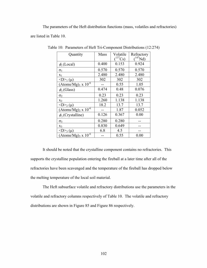
102
The parameters of the Heft distribution functions (mass, volatiles and refractories)
are listed in Table 10.
Table 10: Parameters of Heft Tri-Component Distributions (12:274)
Quantity Mass Volatile ( P
137PCs)
Refractory ( P
147PNd)
1φ (Local) 0.400 0.153 0.924 σB1B 0.570 0.570 0.570 xB1 B 2.480 2.480 2.480 <D>B1 B (µ) 302 302 302 (Atoms/Mg) B1 B x 10P
-6P -- 0.55 1.05
2φ (Glass) 0.474 0.48 0.076 σB2B 0.23 0.23 0.23 xB2 B 1.260 1.138 1.138 <D>B2 B (µ) 18.2 13.7 13.7 (Atoms/Mg) B2 B x 10P
-6P -- 1.87 0.052
3φ (Crystalline) 0.126 0.367 0.00 σB3B 0.280 0.280 -- xB3 B 0.830 0.649 -- <D>B3 B (µ) 6.8 4.5 -- (Atoms/Mg) B3 B x 10P
-6P -- 0.55 0.00
It should be noted that the crystalline component contains no refractories. This
supports the crystalline population entering the fireball at a later time after all of the
refractories have been scavenged and the temperature of the fireball has dropped below
the melting temperature of the local soil material.
The Heft subsurface volatile and refractory distributions use the parameters in the
volatile and refractory columns respectively of Table 10. The volatile and refractory
distributions are shown in Figure 85 and Figure 86 respectively.

0
0.2
0.4
0.6
0.8
1
1.2
0 0.5 1 1.5 2 2.5 3 3.5 4
Log10(diameter)
dNv/
dx Crystalline Distribution
Glass Distribution
Local Distribution
Figure 85: Volatile Distribution for Heft Tri-Component Surface Burst Fallout Particles
0
0.1
0.2
0.3
0.4
0.5
0.6
0.7
0.8
0 0.5 1 1.5 2 2.5 3 3.5
Log10(diameter)
dNr/d
x
4
Glass Population
Local Population
Figure 86: Refractory Distribution for Heft Tri-Component Subsurface Burst Fallout Particles
103

While the local distribution is only approximately 40% of the mass as compared
with 47.4% for the glass distribution, it dominates the refractories, giving the local
distribution more activity per unit mass than the glass distribution. In addition, the Heft
distribution minimizes the amount of activity associated with the crystalline distribution
by not giving it any activity at all from refractories and only 36.7% of the activity
associated with the volatiles even though the crystalline distribution is 17% of the
activity.
104

105
Appendix C. Summary of Surface Effects in SCIPUFF
The conservation of mass equation used by SCIPUFF is
( )Rs FFdtdQ
+−= (C-1)
where
Q is mass,
t is time,
FBs B is the flux of particles at the surface,
FBR B is the flux of particles due to rain scavenging (21:56)
The flux of particles at the surface is defined by:
∫ ==0zDs cdAvF .
where
vBDB is the downward velocity which for particulates is a summation of the average
fall speed of the particle,vBg B, and the deposition velocity of the particle,vBd B (21:56).
For larger particles, vBDB is dominated by the average fall speed of the particles.
The deposition velocity becomes more important the smaller the particle is.
Dry deposition takes into account mechanisms other than gravity and precipitation
that deposit particles from the Gaussian puffs transported by SCIPUFF to the ground or
other surface such as vegetation. Dry deposition is described using the deposition
velocity, vBd B. The deposition velocity is defined at a specific reference height which is
either the vegetative canopy or a height above the surface. For particles, the dry
deposition velocity is found using the following equation:

106
( )⎟⎟⎠
⎞⎜⎜⎝
⎛ −+
+=
0
2/12*
2*
1lnz
zzvuEv
drd
κ (C-2)
where
*u is the surface friction velocity,
*v is the average local friction speed,
κ is the Von Karmans constant (0.4),
zBrB is the reference height,
zB0B is the surface roughness length,
zBdB is the displacement length (20:52).
Finally, E is the collection efficiency which is defined by
( )( )( )IMINB EEEE −−−−= 1111 (C-3)
where
EBB B is the efficiency of the viscous sublayer flow within a millimeter of the surface
elements,
EBINB is the particle interception,
EBIMB is particle impaction (21:52).
The variables that make up the collection efficiency are dependent upon the
surface over which the particles are falling. For vegetative canopies, such as leaves or
grass, where Brownian motion is important, the variables are defined as follows
7.0−= ScfE DB (C-4)
where

107
fBDB is the ratio of the viscous drag to the total canopy drag including pressure
forces. This is assumed to be 1/3,
Sc is the Schmidt number (21:53).
( )⎥⎥⎦
⎤
⎢⎢⎣
⎡⎟⎟⎠
⎞⎜⎜⎝
⎛
+−+⎟
⎟⎠
⎞⎜⎜⎝
⎛
+=
Lp
p
sp
pIN Ar
rf
Arr
fE 1 (C-5)
where
f is the fraction of total particles intercepted by collectors,
r BpB is the radius of the particle,
ABs B is the characteristic radius of small collectors such as vegetative hairs and
ABLB is the characteristic radius of large collectors.
SCIPUFF assumes a value of 0.01 for f, 10 mm for ABs B and 100 mm for ABL B(21:54).
2
2
1 StStEIM +
= (C-6)
where
St is the Stokes number (21:54).
SCIPUFF makes a simplifying assumption and finds the average collection
efficiency, E , in order to find the average local deposition rate.
( ) ββ +−=
EEE
1 (C-7)
where
b is a coefficient between 0.1 and 0.3 that varies with canopy type and velocity
profile (21:54).

108
In addition to the special formulas for collection efficiency SCIPUFF assumes for
vegetative canopies, SCIPUFF assumes the following relationships for vegetative
canopies:
2c
dhz = (C-8)
cr hz 2= (C-9)
where
hBcB is the height of the vegetative canopy (21:55).
For rough surfaces that do not include a vegetative canopy, such as bare soil,
rock, etc., there is no interception, so EBINB is zero. The other collection efficiency terms
are defined as follows (21:55):
7.08.0 −= ScEB (C-10)
IM
IMIM A
AE+
=1
(C-11)
where
( )StIM eStA 42.0108.0 −−= (C-12)
For a rough surface, zBd B is assumed to be zero and z BrB is assumed to be 10m (21:55).
The end result of the dry deposition processes is that the deposition velocity is then added
to the fall velocity and thereby impacts the mass flux at the surface which is used by
SCIPUFF in its conservation of mass equation.
HPAC offers several surfaces over which fallout particles may fall. These
surfaces along with relevant data associated with each surface are presented in table C-1

Table C-1: HPAC Surface Parameters
Surface Canopy Height or Surface Roughness Bowen Ratio Albedo
Desert 0.01 m 4.0 0.3
Urban 0.5 m 1.5 0.16
Cultivated 1 m 0.6 0.16
Grassland 0.25 m 0.9 0.2
Forest 10.0 m 1.0 0.12
Water Roughness = 0.0005 m 0.11 0.12
The Albedo is a measure of the reflectivity of a surface. Specifically, it is the
measure of the radiation of the sun that is reflected to that incident upon a surface.
Albedo is a fraction between 0 and 1. The more reflective a surface is, the higher the
albedo it has. Therefore snow, which tends to reflect a good portion of the sun’s
radiation incident upon it, usually has an albedo of about 0.9. In the realm of fallout
transport, a low albedo would indicate that a surface is likely to retain radiation from the
sun and therefore warm up. This increased temperature at the surface will cause small
thermals which would keep the smaller particles suspended for a longer period of time
than would otherwise occur.
The Bowen Ratio is the ratio of heat conduction to evaporative flux at the air-
water interface. This indicates how much moisture is at the surface compared with the
amount of heat conduction. A high Bowen ratio is usually fairly typical of dry surfaces
while a low Bowen ratio is more typical of moist surfaces.
109

The single most important factor for the surfaces considered here is the canopy
height of the surface. The friction that resists a passing wind encounters is directly
proportional to the canopy height. This friction causes things such as eddies and
turbulence which in turn slows down the rate of travel of the transported puffs. A higher
friction therefore acts to enhance the particle collection efficiency of surfaces with high
canopies. Thus, the higher the canopy is for a particular surface, the more concentrated
the fallout will be over that surface.
110

Appendix D. Code for Calculating g(t)
!*******************************Program HPAC G(t) Maker******************************** Program HPAC_G_t_Maker !************************************************************************************* ! Programer: Timothy Skaar ! Purpose: This program calculates approximate G(t) for HPAC constant wind dose rate fallout
!contour ! Last updated 16 November 2004 ! Last update was to improve integration scheme from Trapezoid to ! Last updated 19 November 2004 ! EW resolution problem found and fixed. ! Updated 23 Nov 2004 - Integration Schemes updated ! Updated 1 Dec 2004 - Lat/Long output fixed
! Updated 16 Dec 2004 - New Lat/Long coordinates added to 1kt Heft to account for Change in Spatial Domain
! Updated 22 Dec 2004 - New Lat/Long coordinates added for 100kt Heft & DELFIC Use Kinds Implicit None Character(len=40)::filename, output_filename Real(dp)::North_Lat Real(dp)::South_Lat Real(dp)::East_Long Real(dp)::West_Long Real(dp)::Grd_Zero_Long Real(dp)::Grd_Zero_Lat Real(dp)::x_resolution, y_resolution Real(dp)::dose_rate_time ! Time dose rate evaluated at in HPAC run Real(dp)::kph ! Wind Speed used in HPAC run Real(dp)::Yield ! [kilotons] Real(dp)::NS_Resolution, EW_resolution ! Resolution (miles then later km) Real(dp)::Longitude_Resolution ! Resolution of Longitude Real(dp)::Starting_Longitude ! Longitude when time is started after grd zero Integer::Long_index ! Index which relates Starting_longitude to dose rate Integer::G_Counter, G_index ! Used for reading 4.03 files Integer::Dimension_Choice Real(dp)::NS_distance, EW_distance ! Dimensions of fallout grid in miles Real(dp),parameter::deg_per_rad = 57.29577951_dp Real(dp)::A,B,C,D ! These are used in lat/long to dist equation Character(len=40)::scratch,scratchdos,scratchtres, scratchquatro Character(len=10)::First_Point Real(dp)::scratch1, scratch2, scratch3 Integer::i,j Integer::ierror
111

Real(dp), allocatable, dimension(:,:)::dose_rate ![rad/hr] Real(dp), allocatable, dimension(:)::Integrate_URDR ! Integrated Unit Reference Dose Rate [R/hr/km] Real(dp), allocatable, dimension(:,:)::Unit_Reference_Dose_Rate !Real(dp), parameter::k=8445._dp ! Surface normalization value [r-km^2/hr-KT] ! There are several possible options for this value. See Bridgman 436 Real(dp)::k Real(dp), allocatable, dimension(:)::G_t !Fractional arrival rate of activity [1/hr] Real(dp), allocatable, dimension(:)::t ! Time [hr] Real(dp)::Distance ! [km] Integer::HPAC_Version Real(dp)::h,XI0, XI1, XI2, X ! Variables for Composite Simpson's rule Integer::Simpson_index Real(dp)::Integrate_G_t Real(dp)::Test_Integrate ! Note 1 R=0.88rad !************************************************************************************************* !The following section of code inputs the long/lat field and calculates resolution and dist. Write(*,*)"Enter Dimension Choice" Write(*,*)"1) 1kt Delfic DR" Write(*,*)"2) 1kt Heft DR" Write(*,*)"3) 10kt Delfic DR" Write(*,*)"4) 10kt Heft DR" Write(*,*)"5) 100kt Delfic DR" Write(*,*)"6) 100kt Heft DR" Write(*,*)"7) User Input Dimension" Read(*,*) Dimension_Choice Select Case (Dimension_Choice) Case(1) !1 kt Delfic DR North_Lat = 33.58611_dp East_Long = -82.91225_dp South_Lat = 33.31649_dp West_Long = -84.26616_dp Case(2) !1 kt Heft DR North_Lat = 33.54073_dp East_Long = -82.92603_dp South_Lat = 33.35937_dp West_Long = -84.25365_dp Case(3) ! 10kt Delfic DR North_Lat = 33.69978_dp East_Long = -81.60902_dp South_Lat = 33.16964_dp
112

West_Long = -84.29636_dp Case(4) ! 10kt Heft DR North_Lat = 33.62621_dp East_Long = -82.78434_dp South_Lat = 33.27465_dp West_Long = -84.25769_dp Case(5) ! 100kt Delfic DR North_Lat = 34.101_dp East_Long = -79.5_dp South_Lat = 32.79871_dp West_Long = -84.34637_dp Case(6) ! 100kt Heft DR North_Lat = 33.93053_dp East_Long = -80.84596_dp South_Lat = 32.98986_dp West_Long = -84.34596_dp Case (7) Write(*,*)"Enter Northern Latitude" Read(*,*)North_Lat Write(*,*)"Enter Eastern Longitude" Read(*,*)East_Long Write(*,*)"Enter Sourthern Latitude" Read(*,*)South_Lat Write(*,*)"Enter Western Longitude" Read(*,*)West_Long End Select Write(*,*)"North Lat is",North_Lat Write(*,*)"East Long is", East_long Write(*,*)"South Lat is", South_lat Write(*,*)"West Long is",West_Long Write(*,*)"Enter Ground Zero Latitude" Read(*,*)Grd_Zero_Lat Write(*,*)"Enter Ground Zero Longitude" Read(*,*)Grd_Zero_Long Write(*,*)"Enter x resolution" Read(*,*)x_resolution Write(*,*)"Enter y resolution" Read(*,*)y_resolution Write(*,*)"Enter Yield" Read(*,*)Yield Write(*,*)"Enter time of dose rate (hrs)" Read(*,*)dose_rate_time Write(*,*)"Enter wind speed (kph)"
113

Read(*,*)kph Write(*,*)"Enter source normalization constant [(R/hr)km^2 per KT at 1 hr](k)" Read(*,*)k !*************************************************************************************************** ! This section is if several runs are to be done and user doesn't want to constantly input data ! Make sure you turn of the read statements in the above section if user wants to use this Grd_Zero_Long=-84.23_dp Grd_Zero_Lat=33.45_dp !x_resolution=150._dp !y_resolution=150._dp !dose_rate_time=23.01_dp !kph=10._dp !Yield=10._dp !*************************************************************************************************** North_Lat=North_Lat/deg_per_rad South_Lat=South_Lat/deg_per_rad East_Long=East_Long/deg_per_rad West_Long=West_Long/deg_per_rad ! Find North South Distance in miles A = North_Lat B = East_Long C = South_Lat D = East_Long !(all converted to radians: degree/57.29577951) If (North_Lat==South_Lat) then NS_Distance=0._dp ElseIf (SIN(A)*SIN(C)+COS(A)*COS(C)*COS(B-D) > 1._dp) THEN NS_Distance = 3963.1_dp * ACOS(1._dp) ! solved a prob I ran into. I haven't fully analyzed it yet NS_Distance=NS_distance*1.609344_dp !Convert from miles to km ELSE NS_Distance = 3963.1_dp*ACOS(SIN(A)*SIN(C)+COS(A)*COS(C)*COS(B-D)) NS_Distance=NS_distance*1.609344_dp !Convert from miles to km End If ! Finds East West Distance in Miles A = North_Lat B = East_Long C = North_Lat D = West_Long !(all converted to radians: degree/57.29577951) If (East_Long==West_Long) then EW_distance = 0._dp ElseIf (SIN(A)*SIN(C)+COS(A)*COS(C)*COS(B-D) > 1._dp) THEN EW_Distance = 3963.1_dp*ACOS(1._dp) ! solved a prob I ran into. I haven't fully analyzed it yet EW_Distance = EW_distance*1.609344_dp !Convert from miles to km
114

ELSE EW_Distance=3963.1_dp*ACOS(SIN(A)*SIN(C)+COS(A)*COS(C)*COS(B-D)) EW_Distance = EW_distance*1.609344_dp !Convert from miles to km End If Write(*,*)"NS Distance is", NS_Distance, "miles" Write(*,*)"EW Distance is", EW_Distance, "miles" Write(*,*)"NS distance is",NS_distance," EW distance is ",EW_distance NS_Resolution = NS_distance/(y_resolution - 1._dp) EW_Resolution = EW_distance/(x_resolution - 1._dp) !************************************************************************************************* ! This section of code reads in the input data Write(*,*)"What Version of HPAC was used?" Write(*,*)"1) 4.03 (Delfic Distribution)" Write(*,*)"2) 4.04 (Heft Distribution)" Read(*,*)HPAC_Version Write(*,*)"Enter filename to read data from" Read(*,*)filename Allocate(dose_rate(1:Int(x_resolution),1:Int(y_resolution))) Allocate(integrate_URDR(1:Int(x_resolution))) Select Case (HPAC_Version) Case(1) If (Int(x_resolution).le.100) then G_index = 1000 Else if ((Int(x_resolution).gt.100).and.(Int(x_resolution).le.300)) then G_index = 10000 Else G_index = 100000 End if Open(unit=4, file=filename, status='old', action='read', iostat=ierror) If (ierror.ne.0) then Write(*,*) "The output file is not opening" End if Do i=1,16 Read(4,*)scratch End Do Read(4,*)First_Point
115

Write(*,*)First_Point Backspace(4) Do i=1,Int(x_resolution) Do j=1,Int(y_resolution) If (j==1.and.First_Point.ne."G0") then G_counter = (Int(x_resolution)-1) - (i-1) Elseif (j==1) then G_counter = i-1 Else G_counter = G_counter + Int(x_resolution) End If If (G_counter.lt.G_index) then Read(4,*)scratch,scratchdos,scratch1,scratch2,dose_rate(i,j) dose_rate(i,j)=dose_rate(i,j)/0.88_dp ! converting from rad to R Else Read(4,*)scratch, scratch1, scratch2, dose_rate(i,j) dose_rate(i,j)=dose_rate(i,j)/0.88_dp ! converting from rad to R End if End Do End Do Close(4) Case(2) Open(unit=4, file=filename, status='old', action='read', iostat=ierror) If (ierror.ne.0) then Write(*,*) "The output file is not opening" End If Do i=1,27 Read(4,*) End Do Do j=1,Int(y_resolution) Do i=1,Int(x_resolution)
116

Read(4,*)scratch, scratchdos, scratchtres, scratchquatro, dose_rate(i,j) dose_rate(i,j)=dose_rate(i,j)/0.88_dp ! Converting from Rad to R End Do End Do Close(4) End Select !************************************************************************************************* ! The following section of Code takes the Way-Wigner approximation to find the unit ! time reference Dose Rate Allocate(unit_reference_dose_rate(1:Int(x_resolution),1:Int(y_resolution))) Do i=1,Int(x_resolution) Do j=1,Int(y_resolution) Unit_Reference_Dose_Rate(i,j) = (Dose_Rate(i,j)/dose_rate_time**-1.2_dp) End Do End Do !************************************************************************************************ !This section of code integrates the dose using trapazoid method Write(*,*) "Starting Trapezoid Method" integrate_URDR=0._dp Do i=1,Int(x_resolution) Do j=2,Int(y_resolution) integrate_URDR(i) = integrate_URDR(i) + (NS_resolution/2._dp)*& &(Unit_Reference_Dose_rate(i,j-1) + Unit_Reference_dose_rate(i,j)) End Do End Do !************************************************************************************************ ! This section of code integrates the dose using composite simpson's method ! See Burden & Faires Pg 199 Write(*,*)"Starting Simpson's method" h = NS_distance/(y_resolution-1) Simpson_index=Int(y_resolution) If ((Real(Simpson_index, dp)/2._dp)==Real((Simpson_index/2),dp)) then Simpson_index=Simpson_index-1
117

End if Do i=1, Int(x_resolution) !Write(*,*)"I is",i XI0 = Unit_Reference_dose_rate(i,1) + Unit_Reference_dose_rate(i, Simpson_Index) XI1=0._dp XI2=0._dp Do j=1, Simpson_index-1 ! Write(*,*)"j is",j If ((Real(j, dp)/2._dp)==Real((j/2),dp)) then XI2 = XI2 + Unit_Reference_dose_rate(i,j) Else XI1 = XI1 + Unit_Reference_dose_rate(i,j) End if End Do XI0 = h*(XI0 + 2._dp*XI2 + 4._dp*XI1)/3._dp Integrate_URDR(i) = XI0 If (Simpson_index.ne.Int(y_resolution)) then Integrate_URDR(i)=Integrate_URDR(i) + (NS_resolution/2._dp)*& &(Unit_Reference_Dose_rate(i,Int(y_resolution)-1) + & &Unit_Reference_dose_rate(i,Int(y_resolution))) End if End Do !************************************************************************************************ !Starting Test integration to check value for k Test_integrate=0._dp Do i=2,Int(x_resolution) test_integrate=test_integrate+(EW_resolution/2._dp)*(Integrate_URDR(i-1)+& &Integrate_URDR(i)) End Do Write(*,*)"The old test integrate value is",Test_Integrate !************************************************************************************************* ! This section converts the Unit_Reference_Integrated_Dose_Rate to g(t) and sets up t(i)
118

Longitude_Resolution = ((West_Long-East_Long)*deg_per_rad)/x_resolution Starting_Longitude = West_Long*deg_per_rad Long_index=0 Do i=1, Int(x_resolution) Starting_Longitude = Starting_Longitude - Longitude_Resolution Long_index=Long_index+1 If (Starting_Longitude.gt.Grd_Zero_Long) then Starting_Longitude=Starting_Longitude + Longitude_Resolution Long_index=Long_index-1 Exit End If End Do Allocate(G_t(1:Int(x_resolution))) Allocate(t(1:Int(x_resolution))) Write(*,*)"Starting G_t calculation" G_t=0._dp t=0._dp Distance=0._dp !Write(*,*)"long index is",long_index Do i=Long_index,Int(x_resolution) !Write(*,*)"i is",i G_t(i)=(Integrate_URDR(i)/(Yield*k))*kph If (i.gt.Long_index) then Distance=Distance + EW_resolution t(i)=Distance/kph End If End Do Distance=0._dp Do i=Long_index-1,1,-1 G_t(i)=(Integrate_URDR(i)/(Yield*k))*kph Distance=Distance - EW_resolution t(i)=Distance/kph End Do !*********************************************************************************************** Test_integrate=0._dp h = Abs(t(1)-t(Int(x_resolution)))/(x_resolution-1) Do i=2,Int(x_resolution) test_integrate=test_integrate+(h/2._dp)*(g_t(i-1)+& &g_t(i)) End Do Write(*,*)"The trap g(t) test integrate value is",Test_Integrate !************************************************************************************************* ! This section of code uses composite Simpson's rule to integrate G_t
119

Write(*,*)"Starting G_t integrate routine" h = Abs(t(1)-t(Int(x_resolution)))/(x_resolution-1) !Write(*,*)"I is",i XI0 = g_t(1) + g_t(Int(x_resolution)) XI1=0._dp XI2=0._dp Do i=1, Int(x_resolution) - 1 ! Write(*,*)"j is",j If ((Real(i+1, dp)/2._dp)==Real(((i+1)/2),dp)) then XI2 = XI2 + G_t(i+1) Else XI1 = XI1 + G_t(i+1) End if End Do XI0 = h*(XI0 + 2._dp*XI2 + 4._dp*XI1)/3._dp Integrate_G_t = XI0 !************************************************************************************************* ! This writes the output file Write(*,*)"Enter output filename" Read(*,*)output_filename Open(unit=5, file=output_filename, status='new', action='write', iostat=ierror) If (ierror.ne.0) then Write(*,*) "The output file is not opening" End if Do i=1,Int(x_resolution) Write(5,2001)t(i), g_t(i) 2001 Format(2es16.7) End Do Write(5,*)"Integrate G_t is",Integrate_G_t Write(5,*)"The file data was read from is",filename Write(5,*)"South Lat is",South_Lat*deg_per_rad Write(5,*)"West Long is",West_Long*deg_per_rad Write(5,*)"North Lat is",North_Lat*deg_per_rad
120

Write(5,*)"East Long is",East_Long*deg_per_rad Write(5,*)"Yield is",yield Write(5,*)"Dose Rate Time is ",Dose_rate_time Write(5,*)"Source Normalization constant is ",k Write(5,*)"This run was completed on 30 Nov 04" Close(5) !************************************************************************************************ End Program HPAC_G_t_Maker
121

Appendix E. Code for Calculating the Grounded Source Normalization Constant
Program HPAC_k_maker ! Programer Timothy Skaar ! Purpose: Input dose rate field from HPAC and calculate grounded source normalization constant ! Created on 22 Nov 04 ! Updated 30 Nov 04 - Added Lat/Long field to output Use Kinds Use Lat_Long_converter Use HPAC_Input Implicit None !********************Variables used in Subroutine HPAC_Parameters********************************* Real(dp)::North_Lat Real(dp)::South_Lat Real(dp)::East_Long Real(dp)::West_Long Real(dp)::Grd_Zero_Long Real(dp)::Grd_Zero_Lat Real(dp)::x_resolution, y_resolution Real(dp)::kph ! Wind Speed used in HPAC run Real(dp)::Yield ! [kilotons] Real(dp)::dose_rate_time !************************************************************************************************* Real(dp)::NS_Resolution, EW_resolution ! Resolution (miles) Real(dp)::NS_distance, EW_distance ! Dimensions of fallout grid in miles Real(dp)::Longitude_Resolution ! Resolution of Longitude in whatever units Longitude is in Real(dp)::Starting_Longitude ! Longitude which time is started at (closest long to grd zero) Integer::Long_index ! Index which relates Starting_longitude to dose rate Integer::i,j Real(dp), allocatable, dimension(:,:)::dose_rate ![rad/hr] Real(dp), allocatable, dimension(:,:)::Unit_Reference_Dose_Rate Real(dp)::Distance ! [km] Call HPAC_Parameters(North_Lat,South_Lat, East_Long, West_Long, Grd_Zero_Long,Grd_Zero_Lat,& &x_resolution, y_resolution, dose_rate_time, yield) Write(*,*)"Finished HPAC Parameters Subroutine" NS_distance=Lat_Long_Distance(North_Lat,East_Long,South_Lat, East_Long)*1.609344_dp EW_distance=Lat_Long_Distance(North_Lat,East_Long,North_Lat,West_Long)*1.609344_dp
122

NS_Resolution = NS_distance/(y_resolution - 1._dp) EW_Resolution = EW_distance/(x_resolution - 1._dp) Allocate(dose_rate(1:Int(x_resolution), 1:Int(y_resolution))) Write(*,*)"Starting HPAC Dose Rate Reader Subroutine" Call HPAC_Dose_Rate_Reader(dose_rate, x_resolution, y_resolution, yield) Write(*,*)"Finished Reading input" !************************************************************************************************* ! The following section of Code takes the Way-Wigner approximation to find the unit ! time reference Dose Rate Allocate(unit_reference_dose_rate(1:Int(x_resolution),1:Int(y_resolution))) Write(*,*)"Finished Allocating URDR" Do i=1,Int(x_resolution) Do j=1,Int(y_resolution) Unit_Reference_Dose_Rate(i,j) = (Dose_Rate(i,j)/dose_rate_time**-1.2_dp) End Do End Do Write(*,*)"Finished creating unit_reference_dose_rate" !************************************************************************************************* Call Integrate(EW_distance, NS_distance, EW_resolution, NS_resolution, Int(x_resolution), & & Int(y_resolution), Unit_Reference_Dose_rate, Yield) End Program HPAC_k_maker !************************************************************************************************** Subroutine Integrate(EW_distance, NS_distance, dgx, dgy, nxmap, nymap, Dose_Rate, Yield) ! Integrate routine is 2-D Simpson's from Burden and Faires Implicit None Integer, Parameter:: dp = Selected_Real_Kind(p=14) Real(dp), Intent(in)::NS_distance ! distance in kilometers from the map center to the left map edge Real(dp), Intent(in)::EW_distance ! distance in kilometers from the map center to the lower map edge Real(dp), Intent(in)::dgx ! resolution in kilometers in the x-direction (left to right across map) Real(dp), Intent(in)::dgy ! resolution in kilometers in the y-direction (top to bottom across map)
123

Integer, Intent(in)::nxmap ! number of points in the x direction across the map Integer, Intent(in)::nymap ! number of points in the y direction across the map Real(dp), Dimension(nxmap,nymap), Intent(in)::Dose_Rate Real(dp)::a,b,n,m Real(dp)::h,x,y Real(dp)::J1, J2, J3, HX Real(dp)::K1, K2, K3 Real(dp)::ymax,xmax,ymin,xmin Real(dp)::Q Real(dp)::L Real(dp)::J Real(dp)::k_eff ! Grounded Source Normalization Constant Integer::i, z ymin=0._dp xmin=0._dp a=xmin b=EW_distance n=Real(nxmap-1, dp) m=Real(nymap-1, dp) ! Step One (Page 233) h=(b-a)/n J1=0._dp J2=0._dp J3=0._dp ! Step Two (Page 233) Do i=0,n ! Step Three x=a+i*h ymax=NS_distance xmax=EW_distance HX = (ymax-ymin)/m K1=dose_rate(i+1,1) + dose_rate(i+1, nymap) K2 = 0._dp K3 = 0._dp ! Step Four Do z=1, m-1 ! Step Five y = 0._dp + z*HX Q=dose_rate(i+1,z+1) ! Step Six If ((Real(z, dp)/2._dp)==Real((z/2),dp)) then K2=K2+Q Else K3=K3+Q End if
124

End Do ! Step Seven L= (K1 + 2._dp*K2 + 4._dp*K3)*HX/3._dp ! Step Eight If (i==0.or.i==Int(n)) then J1=J1+L Else If ((Real(i, dp)/2._dp)==Real((i/2),dp)) then J2=J2+L Else J3=J3+L End if End Do ! Step Nine J=h*(J1+2._dp*J2+4._dp*J3)/3._dp !J= dose Write(*,*)"The integrated Dose Rate is ",J k_eff=J/Yield Write(*,*)"The Grounded Source Normalization Constant is",k_eff Return End Subroutine Integrate
125

Module HPAC_Input ! Modified 16 Dec 2004: Updated 1kt Heft Dimensions to reflect change in Spatial Domain Use Kinds Implicit None Public::HPAC_Parameters, HPAC_Dose_Rate_Reader Private Contains Subroutine HPAC_Parameters(North_Lat,South_Lat, East_Long, West_Long, Grd_Zero_Long,Grd_Zero_Lat,& &x_resolution, y_resolution, dose_rate_time, yield) Real(dp), intent(inout)::North_Lat Real(dp), intent(inout)::South_Lat Real(dp), intent(inout)::East_Long Real(dp), intent(inout)::West_Long Real(dp), intent(inout)::Grd_Zero_Long Real(dp), intent(inout)::Grd_Zero_Lat Real(dp), intent(inout)::x_resolution, y_resolution Real(dp), intent(inout)::dose_rate_time ! Time dose rate evaluated at in HPAC run Real(dp), intent(inout)::yield Integer::Dimension_Choice Write(*,*)"Enter Dimension Choice" Write(*,*)"1) 1kt Delfic DR" Write(*,*)"2) 1kt Heft DR" Write(*,*)"3) 10kt Delfic DR" Write(*,*)"4) 10kt Heft DR" Write(*,*)"5) 100kt Delfic DR" Write(*,*)"6) 100kt Heft DR" Write(*,*)"7) User Input Dimension" Read(*,*) Dimension_Choice Select Case (Dimension_Choice) Case(1) !1 kt Delfic DR !North_Lat = 33.60298_dp !East_Long = -82.93110_dp !South_Lat = 33.2173_dp !West_Long = -84.26808_dp North_Lat = 33.58611_dp East_Long = -82.91225_dp South_Lat = 33.31649_dp West_Long = -84.26616_dp Case(2) !1 kt Heft DR
126

! Old Lat Long for HPAC default Spatial Domain !North_Lat = 33.54320_dp !East_Long = -82.90273_dp !South_Lat = 33.32721_dp !West_Long = -84.32642_dp ! New Lat Long for HPAC with User Adjusted Spatial Domain North_Lat = 33.54073_dp East_Long = -82.92603_dp South_Lat = 33.35937_dp West_Long = -84.25365_dp Case(3) ! 10kt Delfic DR North_Lat = 33.69978_dp East_Long = -81.60902_dp South_Lat = 33.16964_dp West_Long = -84.29636_dp Case(4) ! 10kt Heft DR North_Lat = 33.62621_dp East_Long = -82.78434_dp South_Lat = 33.27465_dp West_Long = -84.25769_dp Case(5) ! 100kt Delfic DR !North_Lat = 33.89648_dp !East_Long = -80.22811_dp !South_Lat = 33.01025_dp !West_Long = -84.34988_dp North_Lat = 34.101_dp East_Long = -79.5_dp South_Lat = 32.79871_dp West_Long = -84.34637_dp Case(6) ! 100kt Heft DR ! North_Lat = 33.70267_dp ! East_Long = -81.41802_dp ! South_Lat = 33.18209_dp ! West_Long = -84.29610_dp North_Lat = 33.93053_dp East_Long = -80.84596_dp South_Lat = 32.98986_dp West_Long = -84.34596_dp Case (7) Write(*,*)"Enter Northern Latitude" Read(*,*)North_Lat
127

Write(*,*)"Enter Eastern Longitude" Read(*,*)East_Long Write(*,*)"Enter Sourthern Latitude" Read(*,*)South_Lat Write(*,*)"Enter Western Longitude" Read(*,*)West_Long End Select Write(*,*)"North Lat is",North_Lat Write(*,*)"East Long is", East_long Write(*,*)"South Lat is", South_lat Write(*,*)"West Long is",West_Long Write(*,*)"Enter Ground Zero Latitude" !Read(*,*)Grd_Zero_Lat Write(*,*)"Enter Ground Zero Longitude" !Read(*,*)Grd_Zero_Long Write(*,*)"Enter x resolution" Read(*,*)x_resolution Write(*,*)"Enter y resolution" Read(*,*)y_resolution Write(*,*)"Enter Yield" Read(*,*)Yield Write(*,*)"Enter time of dose rate (hrs)" Read(*,*)dose_rate_time Write(*,*)"Enter wind speed (kph)" !Read(*,*)kph !*************************************************************************************************** ! This section is if several runs are to be done and user doesn't want to constantly input data ! Make sure you turn of the read statements in the above section if user wants to use this Grd_Zero_Long=-84.23_dp Grd_Zero_Lat=33.45_dp !x_resolution=150._dp !y_resolution=150._dp !dose_rate_time=23.01_dp !Yield=10._dp !*************************************************************************************************** Return End Subroutine HPAC_Parameters Subroutine HPAC_Dose_Rate_Reader(dose_rate, x_resolution, y_resolution, yield) ! This subroutine reads in the Dose Rate from HPAC (which is given in rads) and returns ! the dose rate array to the Main Program in Renken
128

Real(dp), intent(in)::x_resolution, y_resolution Real(dp), dimension(x_resolution,y_resolution), intent(inout)::dose_rate Real(dp), intent(in)::Yield Integer::HPAC_Version Character(len=40)::filename Integer::G_Counter, G_index ! Used for reading 4.03 files Integer::ierror Integer::i,j Character(len=40)::scratch,scratchdos,scratchtres, scratchquatro Real(dp)::scratch1, scratch2, scratch3 Character(len=10)::First_Point Write(*,*)"What Version of HPAC was used?" Write(*,*)"1) 4.03 (Delfic Distribution)" Write(*,*)"2) 4.04 (Heft Distribution)" Read(*,*)HPAC_Version Write(*,*)"Enter filename to read data from" Read(*,*)filename Select Case (HPAC_Version) Case(1) If (Int(x_resolution).le.100) then G_index = 1000 Else if ((Int(x_resolution).gt.100).and.(Int(x_resolution).le.300)) then G_index = 10000 Else G_index = 100000 End if Open(unit=4, file=filename, status='old', action='read', iostat=ierror) If (ierror.ne.0) then Write(*,*) "The output file is not opening" End if Do i=1,16 Read(4,*)scratch End Do Read(4,*)First_Point Write(*,*)First_Point Backspace(4) Do i=1,Int(x_resolution) Do j=1,Int(y_resolution)
129

If (j==1.and.First_Point.ne."G0") then G_counter = (Int(x_resolution)-1) - (i-1) Elseif (j==1) then G_counter = i-1 Else G_counter = G_counter + Int(x_resolution) End If If (G_counter.lt.G_index) then Read(4,*)scratch,scratchdos,scratch1,scratch2,dose_rate(i,j) dose_rate(i,j)=dose_rate(i,j)/0.88_dp ! Converts from rad to R !Write(*,*)"G counter is",G_counter !Write(*,*)scratch Else Read(4,*)scratch, scratch1, scratch2, dose_rate(i,j) dose_rate(i,j)=dose_rate(i,j)/0.88_dp ! Converts from rad to R !Write(*,*)scratch !Write(*,*)"G counter is",G_counter End if End Do End Do Close(4) Case(2) Open(unit=4, file=filename, status='old', action='read', iostat=ierror) If (ierror.ne.0) then Write(*,*) "The output file is not opening" End If Do i=1,27 Read(4,*) End Do Do j=1,Int(y_resolution) Do i=1,Int(x_resolution) Read(4,*)scratch, scratchdos, scratchtres, scratchquatro, dose_rate(i,j)
130

dose_rate(i,j)=dose_rate(i,j)/0.88_dp ! Converts from rad to R End Do End Do Close(4) End Select Return End Subroutine HPAC_dose_rate_reader End Module HPAC_Input
131

Module Lat_Long_Converter Use Kinds Implicit None Public::Lat_Long_Distance Private Contains Function Lat_Long_Distance(Lat1,Long1,Lat2, Long2) Result(distance) ! Purpose ! This subroutine takes a pair of longitude/latitude points and finds the distance ! between them. ! Note 1: Longitude and Latitude points should be input as degrees. ! Note 2: Latitude should always be input as N. Therefore, 33.4S should be input as -33.4N ! Note 3: Longitude should always be input as E. Therefore, 84.23W should be input as -84.23E ! Note 4: Output distance is miles. To convert to kilometers, multiply by 1.609344 Real(dp),parameter::deg_per_rad = 57.29577951_dp Real(dp), intent(in)::Lat1,Long1,Lat2,Long2 ! Latitude and Longitude for points 1 and 2 Real(dp)::Distance Real(dp)::A,B,C,D ! Local Variables A=Lat1/deg_per_rad B=Long1/deg_per_rad C=Lat2/deg_per_rad D=Long2/deg_per_rad If (A==C.and.B==D) then Distance=0._dp ElseIf (SIN(A)*SIN(C)+COS(A)*COS(C)*COS(B-D) > 1._dp) THEN Distance = 3963.1_dp * ACOS(1._dp) ELSE Distance = 3963.1_dp*ACOS(SIN(A)*SIN(C)+COS(A)*COS(C)*COS(B-D)) End If End Function Lat_Long_Distance End Module Lat_Long_Converter
132

Module Kinds Implicit None Integer, Parameter:: dp = Selected_Real_Kind(p=14) Real(dp), Parameter::Pi=3.14159265359_dp End Module Kinds
133
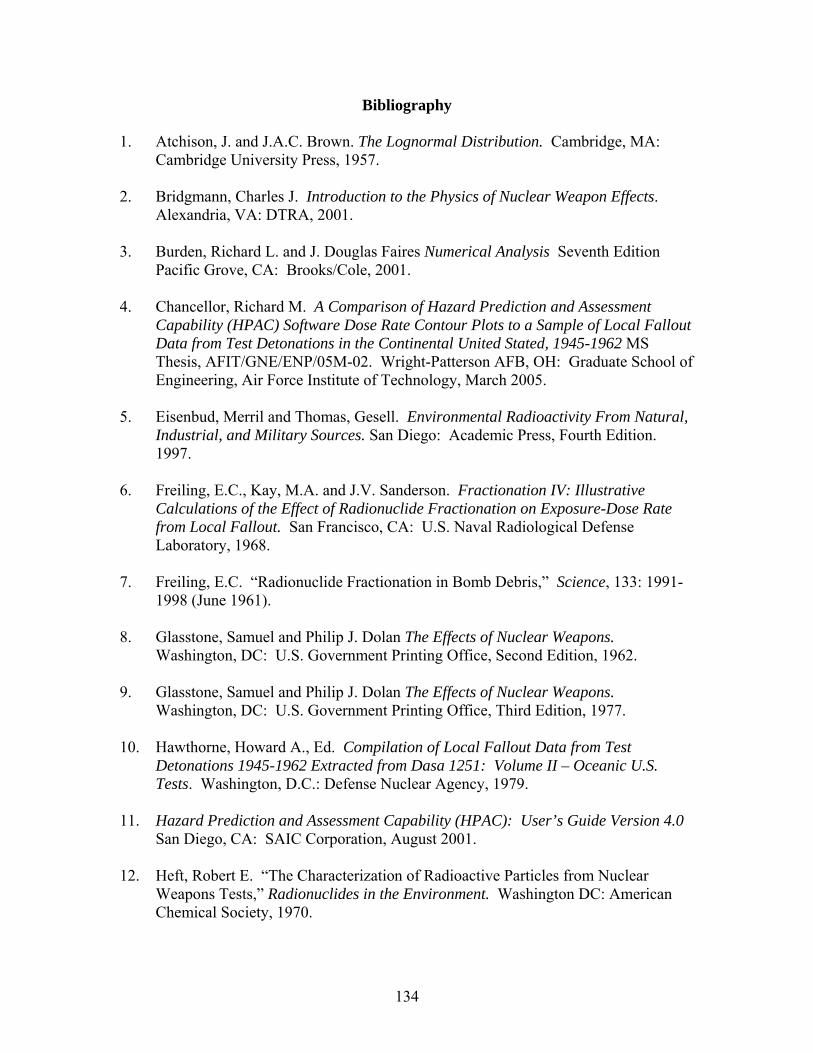
Bibliography 1. Atchison, J. and J.A.C. Brown. The Lognormal Distribution. Cambridge, MA:
Cambridge University Press, 1957. 2. Bridgmann, Charles J. Introduction to the Physics of Nuclear Weapon Effects.
Alexandria, VA: DTRA, 2001. 3. Burden, Richard L. and J. Douglas Faires Numerical Analysis Seventh Edition
Pacific Grove, CA: Brooks/Cole, 2001. 4. Chancellor, Richard M. A Comparison of Hazard Prediction and Assessment
Capability (HPAC) Software Dose Rate Contour Plots to a Sample of Local Fallout Data from Test Detonations in the Continental United Stated, 1945-1962 MS Thesis, AFIT/GNE/ENP/05M-02. Wright-Patterson AFB, OH: Graduate School of Engineering, Air Force Institute of Technology, March 2005.
5. Eisenbud, Merril and Thomas, Gesell. Environmental Radioactivity From Natural,
Industrial, and Military Sources. San Diego: Academic Press, Fourth Edition. 1997.
6. Freiling, E.C., Kay, M.A. and J.V. Sanderson. Fractionation IV: Illustrative
Calculations of the Effect of Radionuclide Fractionation on Exposure-Dose Rate from Local Fallout. San Francisco, CA: U.S. Naval Radiological Defense Laboratory, 1968.
7. Freiling, E.C. “Radionuclide Fractionation in Bomb Debris,” Science, 133: 1991-
1998 (June 1961). 8. Glasstone, Samuel and Philip J. Dolan The Effects of Nuclear Weapons.
Washington, DC: U.S. Government Printing Office, Second Edition, 1962. 9. Glasstone, Samuel and Philip J. Dolan The Effects of Nuclear Weapons.
Washington, DC: U.S. Government Printing Office, Third Edition, 1977. 10. Hawthorne, Howard A., Ed. Compilation of Local Fallout Data from Test
Detonations 1945-1962 Extracted from Dasa 1251: Volume II – Oceanic U.S. Tests. Washington, D.C.: Defense Nuclear Agency, 1979.
11. Hazard Prediction and Assessment Capability (HPAC): User’s Guide Version 4.0
San Diego, CA: SAIC Corporation, August 2001. 12. Heft, Robert E. “The Characterization of Radioactive Particles from Nuclear
Weapons Tests,” Radionuclides in the Environment. Washington DC: American Chemical Society, 1970.
134

13. Krieser, Curtis R. A Rain Scavenging Model for Predicting Low Yield Airburst Weapon Fallout for Operational Type Studies MS Thesis, AFIT/GNE/PH/84M-9. Wright-Patterson AFB, OH: Graduate School of Engineering, Air Force Institute of Technology, Mar 1984.
14. McGahan, Joseph T. Engineer, SAIC, Washington D.C. Personal Correspondance.
13 October 2004. 15. McGahan, Joseph T. “In Cloud Scavening for Low-Intermediate Yields
Preliminary,” Microsoft PowerPoint Presentation, 21 October 2003. 16. McGahan, Joseph T. “Newfall Users Guide and Reference Manual Version 7.5,” 5
March 1996. 17. Morris, Douglass B. A Predictive Technique for Forecasting the Isotopic
Composition of Radioactive Fallout. PhD. dissertation, AFIT/DS/ENP/04-02. Wright-Patterson AFB, OH: Graduate School of Engineering, Air Force Institute of Technology. December 2004.
18. Norment, H.G., Ing, W.Y.G. and J. Zuckerman Department of Defense Land
Fallout Prediction System: Volume II – Initial Conditions Edgewood Arsenal, MD: Defense Atomic Support Agency, 1966.
19. Norment, H.G. DELFIC: Department of Defense Fallout Prediction System Volume
I – Fundamentals. Bedford, MA: Atmospheric Science Associates, 1979. 20. Parker, Edward N. DASA-1188: Radioactive Fallout from Nuclear Explosions
Washington, D.C.: Defense Atomic Support Agency, 1960. 21. Sykes, R.I., Parker, S.F. , Henn, D.S., Cerasoli, C.P. and L.P. Santos PC-SCIPUFF
Version 1.2PD Technical Documentation. Princeton, NJ: Titan Corporation, 1998. 22. Tompkins, Robert C. DASA 1800-V: Department of Defense Land Fallout
Prediction System Volume V – Particle Activity. Edgewood Arsenal, MD: 1968. 23. Wallace, John M. and Peter V. Hobbs Atmospheric Science: An Introductory
Survey. San Diego, CA: Academic Press, 1977.
135

Standard Form 298 (Rev. 8/98)
REPORT DOCUMENTATION PAGE
Prescribed by ANSI Std. Z39.18
Form Approved OMB No. 0704-0188
The public reporting burden for this collection of information is estimated to average 1 hour per response, including the time for reviewing instructions, searching existing data sources, gathering and maintaining the data needed, and completing and reviewing the collection of information. Send comments regarding this burden estimate or any other aspect of this collection of information, including suggestions for reducing the burden, to the Department of Defense, Executive Services and Communications Directorate (0704-0188). Respondents should be aware that notwithstanding any other provision of law, no person shall be subject to any penalty for failing to comply with a collection of information if it does not display a currently valid OMB control number. PLEASE DO NOT RETURN YOUR FORM TO THE ABOVE ORGANIZATION. 1. REPORT DATE (DD-MM-YYYY) 2. REPORT TYPE 3. DATES COVERED (From - To)
4. TITLE AND SUBTITLE 5a. CONTRACT NUMBER
5b. GRANT NUMBER
5c. PROGRAM ELEMENT NUMBER
5d. PROJECT NUMBER
5e. TASK NUMBER
5f. WORK UNIT NUMBER
6. AUTHOR(S)
7. PERFORMING ORGANIZATION NAME(S) AND ADDRESS(ES) 8. PERFORMING ORGANIZATION REPORT NUMBER
9. SPONSORING/MONITORING AGENCY NAME(S) AND ADDRESS(ES) 10. SPONSOR/MONITOR'S ACRONYM(S)
11. SPONSOR/MONITOR'S REPORT NUMBER(S)
12. DISTRIBUTION/AVAILABILITY STATEMENT
13. SUPPLEMENTARY NOTES
14. ABSTRACT
15. SUBJECT TERMS
16. SECURITY CLASSIFICATION OF: a. REPORT b. ABSTRACT c. THIS PAGE
17. LIMITATION OF ABSTRACT
18. NUMBER OF PAGES
19a. NAME OF RESPONSIBLE PERSON
19b. TELEPHONE NUMBER (Include area code)