The Pennsylvania State UniversityThe Graduate SchoolCollege of Engineering

A COMPARISON OF MODELING APPROACHES OF A HIGH

ASPECT CYLINDER IN AXIAL FLOW

A Thesis inEngineering Science and Mechanics

byNicholas LaBarbera

© 2015 Nicholas LaBarbera

Submitted in Partial Fulfillmentof the Requirementsfor the Degree of

Master of Science

December 2015

The thesis of Nicholas LaBarbera was reviewed and approved∗ by the following:

Jonathan S. PittResearch Associate, Applied Research LaboratoryAssistant Professor of Engineering Science and MechanicsThesis Advisor

Robert L. CampbellResearch Associate, Applied Research LaboratoryAssistant Professor of Mechanical Engineering

Judith A. ToddP.B. Breneman Department ChairDepartment of Engineering Science and Mechanics

∗Signatures are on file in the Graduate School.

ii

Abstract

Simulating a fully-coupled fluid-structure interaction system from first-principlescan be very computationally expensive especially for use in design-level analyses;therefore, it is advantageous to explore less computationally expensive methods. Bymaking assumptions about the relevant physics of the problem, simplifications tothe governing equations can be applied. These simplifications result in a reduced-order model that can significantly decrease the computational cost; however, thegoverning equations simplifications result in the reduced-order model neglectingto take into account all the physics of the system. Ideally, the neglected physicswould have little to no impact on the dynamics of the system; however, this is notalways the case for all input parameters. Therefore, it is important to determinethe parameter space for which a reduced order model is valid.

In this thesis, numerical simulations of a slender cylinder in axial flow wereperformed using two different methods. The first is a strongly-coupled fluid-structure interaction simulation based on first-principles. First-principles for thiscase is solving the incompressible Navier-Stokes equations for the fluid and the fullequations of elasticity for the solid domain. The second is a reduced-order model fora cylinder in axial flow that was devised by Paidoussis. It consists of a single linearpartial differential equation that requires significantly less computational resourcesto solve than the non-linear governing equations used in the first-principles model.For certain input parameters, the reduced-order model is capable of predictingstability with comparable accuracy to the first-principles model, but is obtained ina fraction of the time.

The goal of this thesis is to investigate the parameter space for which the lesscomputational expensive reduced order model can be utilized and for which themore computationally expensive first-principles solver is required. To accomplishthe goal, the two models were compared through the variation of input parametersto determine the parameter ranges corresponding to agreement between models.Results are presented and conclusions discussed.

iii

Table of Contents

List of Figures vi

List of Tables viii

List of Symbols ix

Acknowledgments xi

Chapter 1Introduction 11.1 Introduction . . . . . . . . . . . . . . . . . . . . . . . . . . . . . . . 1

Chapter 2Literature Review 52.1 Introduction . . . . . . . . . . . . . . . . . . . . . . . . . . . . . . . 52.2 Existing Models . . . . . . . . . . . . . . . . . . . . . . . . . . . . . 9

2.2.1 String Approximation . . . . . . . . . . . . . . . . . . . . . 102.2.2 Beam Modelling . . . . . . . . . . . . . . . . . . . . . . . . . 112.2.3 Coupled FSI Simulations . . . . . . . . . . . . . . . . . . . . 132.2.4 Recap by Decade . . . . . . . . . . . . . . . . . . . . . . . . 14

2.3 State of the Art . . . . . . . . . . . . . . . . . . . . . . . . . . . . . 162.3.1 Plan to Advance State of the Art . . . . . . . . . . . . . . . 16

Chapter 3First Principle solver 173.1 Introduction . . . . . . . . . . . . . . . . . . . . . . . . . . . . . . . 173.2 Governing equations . . . . . . . . . . . . . . . . . . . . . . . . . . 183.3 Solvers . . . . . . . . . . . . . . . . . . . . . . . . . . . . . . . . . . 18

3.3.1 Solid Solver - FEANL . . . . . . . . . . . . . . . . . . . . . 193.3.2 Fluid Solver - OpenFOAM . . . . . . . . . . . . . . . . . . . 19

iv

3.3.2.1 Derivation of pressure equation . . . . . . . . . . . 203.3.2.2 IcoFoam Algorithm . . . . . . . . . . . . . . . . . . 21

3.4 Verification and Validation . . . . . . . . . . . . . . . . . . . . . . . 22

Chapter 4Reduced-Order Model 254.1 Equation of Motion . . . . . . . . . . . . . . . . . . . . . . . . . . . 254.2 Implementation . . . . . . . . . . . . . . . . . . . . . . . . . . . . . 27

4.2.1 Spatial Discretization . . . . . . . . . . . . . . . . . . . . . . 294.2.2 Temporal Discretization . . . . . . . . . . . . . . . . . . . . 30

4.3 Verification . . . . . . . . . . . . . . . . . . . . . . . . . . . . . . . 314.3.1 Review of Method of Manufactured Solutions . . . . . . . . 314.3.2 Verification . . . . . . . . . . . . . . . . . . . . . . . . . . . 31

4.4 Best Practices . . . . . . . . . . . . . . . . . . . . . . . . . . . . . . 36

Chapter 5Model Comparison 395.1 Introduction . . . . . . . . . . . . . . . . . . . . . . . . . . . . . . . 395.2 Comparison case . . . . . . . . . . . . . . . . . . . . . . . . . . . . 39

5.2.1 Reduced-Order Model Setup . . . . . . . . . . . . . . . . . . 405.2.2 First Principles Simulation Setup . . . . . . . . . . . . . . . 40

5.3 Clamped-free with a blunt end comparison . . . . . . . . . . . . . . 425.4 Clamped-free with a streamlined end comparison . . . . . . . . . . 44

5.4.1 U=1 . . . . . . . . . . . . . . . . . . . . . . . . . . . . . . . 465.4.2 U=2 . . . . . . . . . . . . . . . . . . . . . . . . . . . . . . . 465.4.3 U=4 . . . . . . . . . . . . . . . . . . . . . . . . . . . . . . . 495.4.4 U=6 . . . . . . . . . . . . . . . . . . . . . . . . . . . . . . . 52

Chapter 6Conclusions 566.1 Summary of Work Performed . . . . . . . . . . . . . . . . . . . . . 566.2 Future Work . . . . . . . . . . . . . . . . . . . . . . . . . . . . . . . 57

Appendix ANon Technical Abstract 59

Bibliography 61

v

List of Figures

1.1 Flow chart outlining the thesis . . . . . . . . . . . . . . . . . . . . . 4

2.1 A typical towed array . . . . . . . . . . . . . . . . . . . . . . . . . . 62.2 A towed array close up . . . . . . . . . . . . . . . . . . . . . . . . . 62.3 A picture to show the difference between the continuous distribution

of mass in the beam model(top) as opposed to the lumped massesfound in the cable model (bottom). . . . . . . . . . . . . . . . . . 13

3.1 FSI flow chart . . . . . . . . . . . . . . . . . . . . . . . . . . . . . . 193.2 PISO flow chart . . . . . . . . . . . . . . . . . . . . . . . . . . . . . 223.3 Long Turek setup . . . . . . . . . . . . . . . . . . . . . . . . . . . . 233.4 Vertical tip displacement of Turek cases with different tail lengths . 24

4.1 Physical diagram for the Paidoussis Model . . . . . . . . . . . . . . 274.2 L2 error for displacement for grid refinement study . . . . . . . . . 354.3 L∞ error for displacement for grid refinement study. . . . . . . . . . 354.4 Schematic of vibrating string . . . . . . . . . . . . . . . . . . . . . . 364.5 Backward-Euler Energy Graph . . . . . . . . . . . . . . . . . . . . . 384.6 θ = 0.5 Energy Graph . . . . . . . . . . . . . . . . . . . . . . . . . 38

5.1 Paidoussis Experimental Pictures . . . . . . . . . . . . . . . . . . . 425.2 Schematic of first principle simulation with a blunt tail . . . . . . . 435.3 Grid used for a first principle simulation with a blunt tail . . . . . . 435.4 Tip displacement for full order model with blunt tail and U=4 m/s 445.5 Schematic of first principle simulation with a streamlined tail . . . . 455.6 Grid used for a first principle simulation with a streamlined tail . . 455.7 Tip displacement for full order model with streamlined tail at U=1

m/s . . . . . . . . . . . . . . . . . . . . . . . . . . . . . . . . . . . 465.8 Full order simulation with streamlined tail at U=2 m/s at various

times . . . . . . . . . . . . . . . . . . . . . . . . . . . . . . . . . . . 48

vi

5.9 Tip displacement for full order model with streamlined tail at U=2m/s . . . . . . . . . . . . . . . . . . . . . . . . . . . . . . . . . . . 49

5.10 Full order simulation with streamlined tail at U=4 m/s at varioustimes . . . . . . . . . . . . . . . . . . . . . . . . . . . . . . . . . . . 50

5.11 Tip displacement for full order model with streamlined tail at U=4m/s . . . . . . . . . . . . . . . . . . . . . . . . . . . . . . . . . . . 51

5.12 Tip displacement for both models with streamlined tail at U=4 m/s 515.13 Full order simulation with streamlined tail at U=6 m/s at various

times . . . . . . . . . . . . . . . . . . . . . . . . . . . . . . . . . . . 525.14 Tip displacement for full order model with streamlined tail at U=6

m/s . . . . . . . . . . . . . . . . . . . . . . . . . . . . . . . . . . . 535.15 Tip displacement for both models with streamlined tail at U=6 m/s 535.16 Tip displacement for full order model with streamlined tail at

U=1,2,4,6 m/s . . . . . . . . . . . . . . . . . . . . . . . . . . . . . . 55

vii

List of Tables

2.1 Prakla Array Information . . . . . . . . . . . . . . . . . . . . . . . 7

3.1 Dimensions for the standard and long Turek cases . . . . . . . . . . 23

4.1 Refinement table for verification of y . . . . . . . . . . . . . . . . . 334.2 Refinement table for verification of w . . . . . . . . . . . . . . . . . 334.3 Refinement table for verification of u . . . . . . . . . . . . . . . . . 344.4 Refinement table for verification of v . . . . . . . . . . . . . . . . . 34

5.1 A recap of the results of all the comparison cases performed. . . . . 55

viii

List of Symbols

E Young’s Modulus

I Moment of Inertia

U Free-stream speed of the fluid

D Diameter of the cylinder

L Length of the cylinder

m mass per unit length of the cylinder

M Mass of the displaced fluid

ct Longitudinal drag coefficient

cn Normal drag coefficient

c2 Base drag coefficient

f Measure of tail piece slenderness

l Length of tail piece

t time

ρ density

p pressure

µ viscosity

u fluid velocity vector

ix

um mesh velocity

S Second Piola-Kirchhoff stress

E Lagrangian Green strain

λ Lame Constant

y Displacement of the cylinder

w Slope of the cylinder

u Curvature of the cylinder

v velocity of the cylinder

x

Acknowledgments

I would like to acknowledge Naval Sea Systems Command Advanced SubmarinesSystems Development Office (SEA 073R) and the Penn State Applied ResearchLaboratory for funding to conduct this research. I also owe a major thanks to Dr.Jonathan Pitt & Dr. Scott Miller for advising during this research. Without theirhelp and guidance, this thesis wouldn’t have been possible. Finally, I would liketo thank my family for encouraging me to go back to school to pursue a graduatedegree.

xi

Chapter 1 |Introduction

1.1 IntroductionComputational mechanics has played an important role in the engineering designprocess over the past few decades by providing the necessary tools to go from amathematical model of a complex system to its predicted behavior. The role ofcomputational mechanics is likely to only expand as advancements continue to bemade in both software and hardware.

Increases in computational resource availability have made it possible to simulateproblems and phenomenon that were once too computationally expensive. Inparticular, the demand for coupled multi-physics simulations has been increasingover the years. A multi-physics simulation couples different physical models intoa single model. An example would be coupling thermal effects with a structure’smechanical response.

This thesis focuses on the specific multi-physics problem of fluid-structureinteraction (FSI). A fluid-structure interaction simulation couples the governingequations of solid mechanics with the governing equations of fluid mechanics. Fluid-structure interaction is characterized by the interaction of a deformable solid whosedeformation is dependent on the fluid’s flow field and a fluid whose flow field isdependent on the solid’s deformation. It is this two-way coupling that exemplifiesthe multi-physics nature of a fluid-structure interaction problem.

The physical world is full of examples of fluid-structure interaction such as atree branch swaying in a breeze or a fish swimming in a stream. There are alsofluid-structure interaction problems of practical engineering interest such as the

1

deformation of wind turbine blades (Bazilevs et al., 2011) and the simulation ofartificial heart valves (Dumont et al., 2007).

This thesis will focus on the particular fluid-structure interaction problem of aslender cylinder in axial flow. It has garnered interest from the research communitydue to its application to heat exchangers, nuclear reactor fuel-element bundles andacoustic streamers (Paidoussis, 2004). A cylinder in axial flow may experiencevibrations, due to shedding vortices impinging on the cylinder downstream, causingself-excitation. It is important for engineers to recognize the potential effects ofthese vibrations especially in closely spaced systems. One scenario where axial flowinduced vibrations must be considered is in the design of closely spaced nuclearcooling rods. If the vibrations are not considered during the design phase, thespacing might be too small and the rods could collide during vibrations (Liu et al.,2012). This can result in fretting and long term problems such as fatigue andstress-corrosion cracking (Paidoussis, 2004). Fluid-structure interaction simulationsmodelled with first-principal approaches can accurately capture the physics ofa system; however, this accuracy comes at a price. It requires solving the fullNavier-Stokes equations for the fluid domain and the equations of elasticity forthe solid domain. The result is a very large set of equations that must be solvedeach time step; requiring significant computational resources and time. Thus, itis advantageous to explore less computationally expensive methods. By makingassumptions about the relevant physics of the problem, simplifications to thegoverning equations can be applied. These simplifications result in a reduced-ordermodel of the system that can significantly decrease the computational cost.

Reduced-order model simulations can run orders of magnitude faster, but bynot basing a model on first-principles, some of the physics are lost and theireffects are not captured. In certain situations, these neglected physics can play asignificant role and result in the reduced-order model producing inaccurate results.In other situations, the physics neglected by the reduced-order model can be of littlesignificance. In these situations, the reduced-order model can produce accuratepredictions but in a fraction of the time.

This thesis starts with a literature review of current modelling efforts for towedarrays and cylinders in axial flow. Next, the Paidoussis reduced order model isdiscussed and its implementation into a finite element solver. After that section,the details on the first principles solver are presented. This is followed by a chapter

2

outlining how the comparison cases are set up and results from the simulations.Finally, conclusions are discussed and directions for future work and research areprovided. This is outlined in Figure 1.1.

The goal of this research is to investigate the parameter space that the reduced-order model provides accurate stability predictions and which parameter space isthe more computationally expensive first-principals model necessary. To do this, afirst principles fluid-structure interaction solver was compared to the Paidoussisreduced-order model for a cylinder in axial flow.

The first principles fluid-structure interaction solver used for comparison is anin-house partitioned solver. A partitioned solver uses seperate solves for the fluidand structural domains. To solve the fluid, the open-source finite-volume solver,OpenFOAM (Jasak, 1996) version 2.2 was used. For the fluid, the incompressibleNavier-Stokes equations are solved. The equations of elasticity for a hyper-elasticsolid are solved using an in-house finite element solver, FEANL (Campbell, 2011).The two domains are coupled using an in-house coupling code.

The reduced-order model implemented is the Paidoussis model (Paidoussis,1973) for a cylinder in axial flow. The governing equation for the Paidoussismodel is linear, and therefore requires much less computational resources to solvenumerically. This speed increase comes at the cost of lost physics. One effect notmodeled is the effect of the cylinder’s deformation on the flow field of the fluid.Also effects such as vortex shedding are neglected. A thorough treatment on thePaidoussis model as well the dynamics of structures in axial flow can be foundin (Paidoussis, 2004). The Paidoussis model was numerically implemented forthe test case using the open-source finite element library Deal.ii (Bangerth et al.,2013). A case for comparison was simulated using both approaches and comparedto determine the range of validity for the reduced-order model.

3

Introduction

Cylinder in axial flow modelling overview

Reduced Order Model Implementation and Verification

Conclusions

Stability Comparisons of the First Principles and Reduced Order Model

First Principles Solver Details

Chapter 1

Chapter 2

Chapter 3

Chapter 4

Chapter 5

Chapter 6

Figure 1.1: A flow chart outlining the work presented in this thesis.

4

Chapter 2 |Literature Review

2.1 IntroductionSonar has found many uses in the world. It can be used to map the seabed fornavigational safety maps and cable-laying routes. The oil-industry uses sonar toto explore for potential drill sites and sonar has long been a standard tool usedby the Navy for target detection (Lemon, 2004). In all these applications, it isbeneficial to have the maximum resolution and range possible. This has lead tothe development of towed sonar-array systems or towed arrays for short.

Towed arrays have superior range and resolution in comparison to hull mountedsonars; however, the effectiveness of a towed array is directly proportional to howprecise the instantaneous location of each individual hydrophone on the array isknown (Gerstoft et al., 2003). Therefore, there exists a need to be able to accuratelypredict the shape of an array under various operating conditions. Towed arrayscan be several kilometers long, which makes performing full-scale experiments anextremely difficult task. Due to the high aspect-ratio of towed arrays, it is difficultto perform scaled model experiments. Thus, computer simulations are the mostfeasible option for predicting array shape and motion.

A towed array is a long, slender cable that is towed hundreds of meters behinda ship. Hydrophones are attached to the cable sufficiently far away from the ship toreduce the amount of noise picked up from the ship itself (Barbagelata et al., 2008).The sensor array is typically 2 to 4 inches in diameter and towed by a cable up to8,000 ft long (Pike, 2013; Lasky et al., 2004). A drawing of a towed array is shownin Figure 2.1. Inside the array are wires to carry data and electricity, hydrophones

5

Figure 2.1: A typical towed array (Zhdanov, 2013)

Figure 2.2: Close up of oil filled towed array used for marine biology research(Gogan, 2014)

to pick up sounds, and oil to make the array neutrally buoyant and to help dissipateheat from the electrical equipment (Pike, 2013; Lasky et al., 2004). This is shownin Figure 2.2. A drogue will sometimes be attached to increase tension and stabilityin the line.

Towed arrays come in different lengths and numbers depending on their intendeduse. The oil exploration field will tow up to 16 arrays at once from a single ship(Lemon, 2004). A few dimensions for towed arrays used for oceanography researchare presented below in Table 2.1.

6

Table 2.1: Details of the Prakla Series of Towed Arrays(Barbagelata et al., 2008)

Parameter Prakla 128 Prakla 256

Year Introduced 1979 1991Array Length 45m 254 mHose Diameter 68 mm 90 mmTow cable length 1000 m 1500 mTow cable diameter 62 mm 25.4 mmNumber of Hydrophones 64 128

There are several advantages of a towed array sonar system over a hull mountedsonar. The first advantage is the reduction in interference noise picked up by thearray. Ships are inherently noisy due to vibrations of the engines, the movement ofthe propellers, and the crashing of waves on the hull. By having the hydrophonesof the array located sufficiently far away from the towing vessel, the towed arraypicks up less interference noise. Thus, the resolution and range of the towed arrayis increased over similar hull mounted sonars (Kopp, 2010). Towed Arrays canalso be positioned at various depths, which gives towed arrays the ability to takeadvantage of ocean conditions with better acoustic properties (Barbagelata et al.,2008).

Another advantage of a towed array is its ability to cover the baffles (Lemon,2004). A baffle is the hull-mounted sonar’s blind spot located directly behind theship. This blind spot is due to the sonar’s ineffectiveness in that region from to thenoise created by the engine and the propeller (Kopp, 2010).

Perhaps the greatest benefit of a towed array is the ability to utilize the techniqueof beamforming. Beamforming allows the numerous hydrophones to work togetherto improve gain as well as resolution (Kopp, 2010). However, beamforming requiresthat the position of each hydrophone on the array be known, and uncertainty inposition results in decreased performance (Barbagelata et al., 2008). One way ofhandling the uncertainty in the shape of the array is to consider the array as alwaysbeing in a straight line (Lu et al., 2003), but ocean currents and maneuvering bythe towing ship can cause the shape of the array to deviate from being linear (Luet al., 2003). The uncertainty in the sensor’s position reduces the effectiveness

7

of beamforming, and thus degrades the performance of the array (Gerstoft et al.,2003). There exists a need for the ability to accurately predict an array’s shapeunder various conditions.

There are other disadvantages to using a towed array besides the requirementof knowing the array’s shape. The long length and heavy weight of a towedarray system results in towed arrays requiring large dedicated machinery for theirdeployment and retrieval. This is especially a problem for towed array deploymentfrom vessels where space is limited (Potter et al., 2000). A smaller array diameterwould be lighter and would require smaller machinery for deployment (Barbagelataet al., 2008), but it is difficult to decrease an array’s diameter due to the needfor wires to deliver power and transfer data (Pike, 2013). Complicated telemetryschemes for the internal wiring has been used as a means to reduce the array’sdiameter, but has resulted in higher manufacturing costs and reduced reliability ofthe array (Pike, 2013). The reduction in reliability furthers the need to be able toaccurately predict stresses experienced by the array in various situations.

Another drawback to most single towed arrays is the inability to discern a signal’sdirection. This is because the hydrophones used for towed arrays are omnidirectional(Lemon, 2004). This problem has been addressed by using two towed arrays, a rightand a left array, to discern directivity (Lemon, 2004). Incorporating roll sensorsin the towed array or using hydrophone triplets are alternative methods used fordiscerning directivity (Barbagelata et al., 2008).

Modeling Challenges

Accurately modeling a towed array poses several technical challenges. For example,the aspect ratio for the TB-16 array is roughly 1000:1 (Pike, 2013), and this iswithout factoring in the length from the tow cable. The large aspect ratio and lengthof a towed array makes it difficult to perform experiments to validate simulations( Ni, 1978; Srivastava, 1998; Obligado, 2013). It also presents problems for buildingscale models to be tested in water tunnels and flumes. After scaling the lengthdown to a size that can be tested in a water tunnel, the diameter becomes muchtoo small for accurate scale testing.

A towed array is comprised of different sections made up of different materialswith different properties, which further adds complexity to the problem. Further-

8

more, towed arrays have low bending stiffness which allows them to experiencelarge deviations from a linear configuration.

During maneuvering the flow is not strictly axial flow. Towed arrays experiencea cross flow component as well, and the amount of axial and cross flow can varyalong the length of the array. Cross flow over a cylinder causes vortex sheddingat an increased rate in comparison to axial flow. It is important, and difficult, todetermine to what degree the array is experiencing cross flow and axial flow, forboth self-noise and dynamic analysis.

Natural conditions such as ocean currents and the heaving of the ship by wavesadd stochastic components to the model, while ocean currents add even moredifficulty by varying along the length of the array. These factors all contribute tothe complexity of the system.

2.2 Existing Models

Paidoussis Model

Research on slender and flexible towed bodies began in the 1950’s when W.R.Hawthorne invented the Dracone Barge (Paidoussis, 2004). The Dracone Barge isa long flexible tube used to transport lighter than water liquids (Hawthorne, 1961).The modern Dracone Barge is mainly used to aid in cleaning up oil spills by beinga container that oil is pumped into (Paidoussis, 2004).

Paidoussis, a former graduate student of Hawthorne, built upon Hawthorne’swork and published an analysis of the equations of motion as well as experimentalresults for a fully submerged cylinder in axial flow (Paidoussis, 1968). His model isoften referred to as the "Paidoussis model" or the "Paidoussis equation" (Paidoussis,2004). The equation is a combination of the inviscid forces derived by Lighthill(1960) during his study on the swimming of fish and the viscous forces derivedby Paidoussis (1968). However, Paidoussis’ 1968 paper contained an error in thecalculation of the viscous forces and was corrected in his 1970 paper. The incorrect1968 equation will still produce accurate results for short cylinders in axial flow(Paidoussis, 2004).

The corrected 1970 equation for a uniform cylinder in 2D axial flow is

9

EI∂4y

∂x4 +M( ∂∂t

+ U∂

∂x)2y + 1

2cN(MU

D

)(∂y

∂t+ U

∂y

∂x

)

− 12MU2

[c2 + cT

L− xD

]∂2y

∂x2 +m∂2y

∂t2= 0 (2.1)

where

• EI is the flexural rigidity.

• U is the speed of the fluid.

• D is the diameter of the cylinder.

• L is the length of the cylinder.

• m is the mass per unit length of the cylinder.

• M is the mass of the displaced fluid.

• ct and cn are the longitudinal and normal drag coefficients, respectively.They are typically on the order of magnitude of 0.01. Also the ratio, cn/ctusually ranges between 0.5 for a rough cylinder and 1.5 for a smooth cylinder(De Langre et al., 2007).

• c2 is the base drag coefficient which is typically between 0.1 and 0.7 (Paidoussis,2004). A table of base drag coefficients for various shapes can be found inchapter 10 of (Blevins, 1984).

2.2.1 String Approximation

Given the large aspect ratio of towed arrays, it may be a reasonable approximationto assume there are no internal flexural forces by modeling a towed array as a string(Paidoussis, 2004). This has been investigated by Dowling (1988) and Traintafyllou(1989).

When very long cylinders in axial flow are undergoing vibratory response, thereis a neutral point where the tension caused by drag is equal to the inertial forces(De Langre et al., 2007). Upstream of the neutral point, the cylinder is in tension,but the cylinder is in compression downstream of the neutral point. The neutral

10

point causes a mathematical singularity to arise. This mathematical singularitydoes not arise when using a string model for cylinders shorter than their neutralpoint because the entire cylinder is in tension and there are no points of zerostiffness. Dowling overcame the neutral point phenomenon by using asymptoticexpansions (Dowling, 1988). M.A. Vaz (1995) used this formulation to model atowed array as a string broken into segments to investigate the transient behaviourof a towed array. The results were compared to the full-scale experiments on cablelaying by Hopland (1993) .

Ni & Hansen (1978) conducted experiments for neutrally-buoyant, long, slendercylinders in axial flow. Their results were not in accordance with the string-modelpredictions of Traintafyllou & Chryssostomidis (1989). However, Paidoussis (2004)comments that if you consider the upstream part of the cylinder as rigid dueto tension, then the flexible portion of the cylinder is shorter. The result is adifferent ratio of length to diameter for the flexible portion and can explain thediscrepancies between the experimental observations of Ni & Hansen and thetheoretical predictions of Traintafyllou & Chryssostomidis (Paidoussis, 2004). DeLangre (2007) builds upon this by going into more detail on modeling a longcylinder as rigid until a critical length. His model treats the the portion of thecylinder before the critical length as rigid and the remaining portion as flexible.He models the flexible downstream portion with a simple string model.

An example of a string equation from G.S. Traintafyllou (1989) is displayedbelow.

[MU2 − T0 −12ρDU

2Cf (L− x)]∂2y

∂x2 + 2MU∂2y

∂x∂t+

12ρDUCf

(∂y

∂t+ U

∂y

∂x

)+ (m+M)∂

2y

∂t2= 0 (2.2)

2.2.2 Beam Modelling

To include flexural forces in a towed array model, the towed array must be modelledas a beam. A beam model overcomes the mathematical difficulties encounteredby string models at points of zero tension. This advantage is offset by makingthe numerical model more computational expensive. The reduced order modelimplemented in this thesis falls into the category of a linear beam model. These

11

models are still considered only 1-way coupled because they do not take into accountthe effect the solid’s deformation has on the fluid. Some of the models do useempirical relations to account for the solid’s effect on fluid, such as was done byH.I. Park (2003). Park’s model incorporated drag coefficients that increased withReynolds number to take into account vortex shedding.

An example of a governing equation for a cylinder in axial flow modeled usinga beam is below (Chen, 1970).

EI∂4y

∂x4 + ρAU2 + 14CTρU

2LD∂2y

∂x2 + 12CNρD

∂y

∂t(mρA)∂

2y

∂t2= 0 (2.3)

A subcategory of beam models is cable models. Cable models take into accountbending stiffness, as all beam models do, but instead of having the mass continuouslydistributed, it is instead approximated by a network a lumped masses connectedby massless connections (Gobat, 2006). This is shown in Figure 2.3. Each mass isa rigid body with both rotational and translational degrees of freedom. The resultof making this approximation is the ability to apply the Newton-Euler equationsof motion for each individual mass to obtain a system of equations without theappearance spatial derivatives. The connecting sections are modelled as a collectionof massless linear and torsion spring/damper systems to account for stretching andtorsional forces in the cable (Gobat, 2006). Furthermore, it is possible to modelanisotropic materials by modeling the system as a set of spring/damper systemsin different planes with different properties (Orcina, 2013). By adding additionalmodeling to the system, cable models can simulate things such as contact andhysteresis.

The advantage of cable models are that they are more efficient than solving thefull elasticity equations. Time-savings are also reaped by decoupling the solid’seffect on the fluid’s flow field. The price of these speed increases is a loss of accuracywhen compared to a fully-coupled simulation that solves the elasticity equationsand the Navier-Stokes equations. It is worth noting that cable models still onlyhave one-way coupling. Specifically, the fluid’s effect on the solid is taken intoaccount, but the solid’s effect on the fluid is ignored. Cable models also do notdirectly model some fluid phenomenon such as vortices being shed by the cable.Therefore, a cable model is not a fully-coupled first principles model for a towedarray. Examples of cable models already developed are the Wood’s Hole Oceanic

12

Institute (WHOI) CABLE program (Gobat, 1998) and the commercial programOrcaFlex (Orcina, 2013).

Lumped masses

Cable system

Continuous system

Figure 2.3: A picture to show the difference between the continuous distribution ofmass in the beam model(top) as opposed to the lumped masses found in the cablemodel (bottom).

2.2.3 Coupled FSI Simulations

Another modeling approache is to fully couple the fluid and the solid by modelingboth from first principles. For the case of a towed array, the governing equations arethe incompressible Navier-Stokes equations to model the fluid, and the equationsof elasticity to model the solid. The governing equations for a solid and a fluid arecoupled through the use of appropriate boundary conditions on the interface.

A fully coupled fluid-structure interaction simulation from first principles isconsidered computationally expensive because it requires solving a non-linearcoupled system of partial differential equations. The string approximation and thebeam approximations resulted in solving a single linear differential equation, whichis much less computationally demanding.

Research groups have performed full FSI simulations for cylinders in axial flow,but they have been clamped on both ends such as is found in nuclear fuel rods(Liu et al., 2012). There has also been a full FSI simulation of a clamped-freecylinder in axial flow by Fujita & Ohjuma (2010). However, these simulations have

13

a drastically different aspect ratio when compared to a towed array. To the best ofthe author’s knowledge, a full FSI simulation for a towed array or cylinder with asimilar aspect ratio has not been performed or published.

Recently several research groups have carried out full fluid-structure interactionsimulations for axial flow. Z.G. Liu et al. (2012) of Hong Kong Polytechnic Institutehave performed fully coupled simulations of cylinder clusters clamped at both endsunder axial flow. This work was done to better model nuclear cooling rods. However,these simulations have a drastically different aspect ratio when compared to a towedarray and do not have a free downstream end.

2.2.4 Recap by Decade

A cylinder in axial flow is an important fluid-structure interaction problem. Theimportance became apparent in the 1950’s during the design of heat exchangers andcooling rods in nuclear power plants. The axial flow over nuclear cooling rods cancause them to vibrate. If the cooling rods are too closely spaced, they can collideand be damaged. Axial flow induced vibrations can also cause fatigue damage inmaterials. This is especially important for designing and predicting usable life forlong service parts such as nuclear cooling rods.

In the 1960’s two major papers were published. The first was Lighthill’s paperon slender fish swimming, where he derives the inviscid forces on a fish. The otherwas Paidoussis’ 1968 paper on the equation of motion for a flexible cylinder in axialflow and the experiments he conducted.

Paidoussis (1970) corrects an error in his 1968 paper. The error wasn’t foundduring his experiments because it only has importance for long systems, such asa towed array. This was also the decade in which Ni & Hansen (1978) performedexperiments for long slender cylinders in axial flow. Ni & Hansen’s experimentshad an aspect ratio of 500, which is much less than a towed array, but is one of thefew experiments on large aspect ratio cylinders in axial flow.

In the 1980’s, numerical simulations for towed arrays were becoming more com-mon, such as in (Ablow, 1983; Chapman, 1984; Milinazzo et al., 1987; Traintafyllou,1989). This is also the decade when the neutral point singularity of 1-D string modelwas overcome by A.P. Dowling (1988). Chapman (1984) performed simulations forthe response of towed arrays during turns by using a string model that neglected

14

cable stretching and inertial forces.Gagnon and Paidoussis (1994a; 1994b) published papers on the vibration of a

cluster of cylinders in axial flow. These papers contain both theory and experimentalvalidation. Further work was performed on the response of towed arrays duringturns by Vaz & Patel (1995). Calkin (1999) developed a metamodel based offof curve fitting data to previous results from a large matrix of conditions. Thismetamodel was applied to simulations for the AN/SQR-18A towed array, andfull scale sea trials were performed to validate his model. S.K. Srivastava & C.Ganapathy (1998) performed experiments in a wave basin on a towed array modelto investigate the effects of loop maneuvers on the towed array.

Bhattacharyya (2000) used the finite element model for a towed flexible cylinderand used his model to examine the effect the shape of the downstream end has onstability. Gobat (2006; 2007) at the Woods Hole Oceanographic Institution per-formed numerical simulations with their CABLE program to build upon Chapman’swork on the responses of towed array’s during turns. Park’s (2003) simulations oftowed arrays did not directly simulate vortex shedding, but accounted for it byincreasing the drag coefficients accordingly.

Recently several research groups have carried out full fluid-structure interactionsimulations for axial flow. Z.G. Liu (2012) have performed fully coupled simulationsof cylinder cluster clamped at both ends under axial flow. Their work was performedto improve models of nuclear cooling rods. There has also been full FSI simulationson a clamped-free cylinder in axial flow by Fujita & Ohjuma (2010). However, thesesimulations have a drastically different aspect ratio when compared to a towedarray.

There is very little experimental data for cylinder with a length to diameterratio comparable to that of a towed array. One example was performed by M.Obligado & M. Bourgoin (2013). The experiment was for a cable with an aspectratio of 5 x 104 in a wind tunnel. In their experiments, spheres of different weightswere attached to the end and the stability was examined. Their experiment for acable without a sphere attached on the end was compared to the simulation resultsin (De Langre et al., 2007) and was found to agree.

15

2.3 State of the ArtThe majority of simulations for towed cylinders fall into one of three categories.The first is to ignore bending stiffness and model the array as a 1-D string suchas in (Dowling, 1988; Traintafyllou, 1989). The second category is a model whichincorporates bending stiffness. This can be a simple model that treat the towedarray as a uniform cylinder (Bhattacharyya et al., 2000) or more detailed one thatincorporates aspects such as material non-linearities and non-uniform materialproperties along the length of the towed system (Grosenbaugh, 2007). However,none of these models take into account the effect the cylinder has on the flow of thefluid. Park (2003) does consider the effects of vortex shedding; however, the vortexshedding isn’t directly simulated, and instead the drag coefficients are increased toaccount for presumed vortex shedding.

The third category is fully-coupled first-principles simulations. There are firstprinciple simulations for a cylinder in axial flow, but to the author’s knowledge therehas not been a first principles simulation of a cylinder with a high aspect ratio inaxial flow. As was previously stated, these types of simulations are computationallyexpensive in comparison to reduced order models.

2.3.1 Plan to Advance State of the Art

The author plans to advance the state of the art is to evaluate existing modellingtechniques and select one or a combination of approaches that yield the bestcombination of physical realism and computational efficiency. To that end, afirst principles simulation is compared to a published reduced-order model todetermine situations where the reduced order model provides acceptable results.More specifically, this thesis is more interested in identifying areas where thereduced-order model fails to provide accurate results. Future work will then beperformed to devise a reduced order model with a greater range of validity. Anothergoal of this thesis is to help make the decision on which model to use for a simulationby giving guidelines on how to balance accuracy and computational cost.

16

Chapter 3 |First Principle solver

3.1 IntroductionReduced-order models for towed arrays often assume that the flow field is constant;however, this is not the case because as the cylinder deforms it affects the fluidflow. This change in the fluid flow then affects the deformation of the cylinder,as seen in vortex induced vibrations (Paidoussis, 2004). Therefore a fully coupledfluid-structure interaction simulation is generally necessary to capture the effectsof this two way coupling.

There are two approaches to coupling the governing equations for both thesolid and the fluid. The first approach is to solve the equations for the fluid andsolid simultaneously with one solver during each timestep. This approach is calledmonolithic and has been used in several codes such as Michler (2004) and Bazilevs(2008). The second approach is termed the partitioned approach. In the partitionedapproach, separate solvers are used for the fluid and solid domains as was done inCampbell (2011), Matthies (2003), and Kittler (2006). Iterations are performed ateach timestep until the solutions for both the solid and fluid converge to withinsome tolerance. The advantage to a partitioned approach is the ability to usesolvers well-suited to the particular domain they are solving. The FSI solver usedin this thesis uses a partitioned approach. To solve the fluid, the open sourcefinite-volume solver OpenFOAM (Jasak, 1996) was used. The solid solver is anin-house finite element solver, FEANL (Campbell, 2011).

The primary difficulty in partitioned FSI is the efficient coupling of the disparatedomains. This is due to the fact that the equations governing the solid are

17

often formulated from a Lagrangian frame while the fluid equations are oftenformulated using an Eulerian description. Communicating data between the twosets of governing equations is a non-trivial matter, and consequently, our governingequations are formulated using an Arbitrary Lagrangian-Eulerian method, or ALEmethod for short. The ALE method combines both the Lagrangian and Eulerianviews by allowing grid points to move, but not forcing them to stay attached to amaterial point (Donea et al., 1982).

3.2 Governing equationsThe governing equations for the fluid domain are the Navier-Stokes equations foran incompressible fluid. They are written in the ALE form to handle the meshdeformations (Masud, 1997), such that

ρ∂u∂t

+ ρ(u− um) · 5u = −5 p+ µ52 u

5 · u = 0(3.1)

In the ALE N-S equations, ρ, p, t, µ, u, and um represent fluid density, fluidpressure, time, fluid viscosity, fluid velocity, and mesh velocity respectively.

The cylinder is modeled as a hyperelastic solid by using Saint Venant-Kirchhoffmodel. This results in the solid exhibiting elastic behaviour for large deformations.The solid equation is formulated in the Lagrangian frame of reference as

S = λtr(E)I + 2µE (3.2)

where S is the second Piola-Kirchhoff stress and E is the Lagrangian Greenstrain. λ and µ are the Lamé constants.

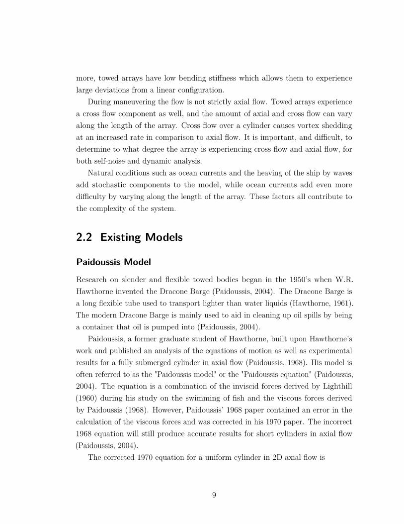
3.3 SolversThe FSI solver uses a partitioned approach. The fluid is solved with the opensource finite-volume solver OpenFOAM that uses the PISO algorithm (Issa, 1986)for an incompressible flow. The solid solver is an in-house finite element solver. Aflow chart of the FSI solver is shown in Figure 3.1.

18

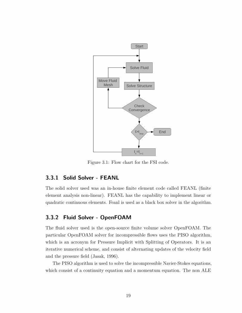
Figure 3.1: Flow chart for the FSI code.

3.3.1 Solid Solver - FEANL

The solid solver used was an in-house finite element code called FEANL (finiteelement analysis non-linear). FEANL has the capability to implement linear orquadratic continuous elements. Feanl is used as a black box solver in the algorithm.

3.3.2 Fluid Solver - OpenFOAM

The fluid solver used is the open-source finite volume solver OpenFOAM. Theparticular OpenFOAM solver for incompressible flows uses the PISO algorithm,which is an acronym for Pressure Implicit with Splitting of Operators. It is aniterative numerical scheme, and consist of alternating updates of the velocity fieldand the pressure field (Jasak, 1996).

The PISO algorithm is used to solve the incompressible Navier-Stokes equations,which consist of a continuity equation and a momentum equation. The non ALE

19

Navier Stokes equations are

∇ · u = 0 (continuity) (3.3)∂u∂t

+∇ · (u⊗ u)−∇ · (ν∇u) = −∇p (momentum) (3.4)

The non-linearity in the convection term is solved iteratively with the followingapproximation

∇ · (u⊗ u) ≈ ∇ · (u0 ⊗ un) (3.5)

In this case u0 is the currently available solution and un is the new solution. Thealgorithm repeats until u0 ≈ un (Jasak, 1996). A flow chart illustrating the PISOalgorithm is shown in Figure 3.2.

3.3.2.1 Derivation of pressure equation

A difficulty with solving the incompressible Navier-Stokes is the lack of a pressureequation. Issa (1986) derived a pressure equation using the momentum equationsand the continuity equation. The semi-discretized momentum equation is

apUp + Σanun −u0

∆t = −∇p. (3.6)

A simplification is made by introducing

H(u) = −Σanun + −u0

∆t . (3.7)

The result isapup = H(u)−∇p, (3.8)

which after dividing by ap is

up = ( 1ap

)(H(u)−∇p). (3.9)

Substituting this into the continuity equation, the pressure equation is obtained,

∇ · [( 1ap

)(H(u)−∇p)] = 0, (3.10)

20

which is rearranged to arrive at the elliptic equation for p,

∇ · [( 1ap

)∇p] = ∇ · [( 1ap

)H(u)]. (3.11)

3.3.2.2 IcoFoam Algorithm

The PISO algorithm is used by the specific OpenFOAM solver called IcoFOAM.IcoFOAM uses the following algorithm to solve the fluid domain.

1. First set boundary conditions for the problem.

2. Next discretize and solve the momentum equation,

∂u∂t

+∇ · (uφ)−∆(ν∇u) = −∇p, (3.12)

to compute an intermediate velocity field where the pressure from the previoustime step is used, and φ is the flux of u from the last known value of u.

3. Then store the discretization coefficients, ap, from the last solution for velocity.

4. Store the velocity solution without the pressure gradient by using

u = 1ap

H(u), (3.13)

and use this approximate velocity to calculate the interpolated face fluxes, φ.

5. Then calculate the new pressure,

∆( 1app) = ∇ · (φ). (3.14)

6. Correct the approximate velocity field by subtracting off the pressure gradientas a corrector

U− = 1ap∇ · p, (3.15)

and update the boundary conditions.

7. If the solution is unconverged, return to step 3, otherwise move to the nexttime step.

21

Solve DiscretizedMomentum Equation

Calculate Mass Flux

Solve Pressure Correction Equation

Correct Velocities andUpdate Bcs

Correct Mass Flux

CheckConvergence

No

Set BCs

Next Timestep

Yes

Figure 3.2: Flow chart for the PISO Algorithm.

3.4 Verification and ValidationThe first principles solver has been verified and numerically validated by comparingto the Turek and Hron benchmark case shown in Figure 3.3 (Miller et al., 2014;Turek, 2006). The Turek-Hron benchmark case consists of a rigid and fixed cylinderin channel flow with a flexible trailing tail. The inlet velocity profile is parabolicand the cylinder is slightly off center to encourage the shedding of vortices. Asvortices are shed from the cylinder they impinge on the flexible tail and excite itinto vibration. A table of model properties is given in Table 3.1.

22

Figure 3.3: The setup for the long Turek case consists of channel flow with aparabolic inlet velocity. The cylinder is rigid and fixed in place. Attached to thecylinder is a flexible tail, and displacements are measured at the tip of the tail

Geometry parameters Standard Turek case [m] Long Turek case [m]channel length 2.5 4.5channel width 0.41 0.41

cylinder center position (0.2,0.2) (0.2,0.2)cylinder radius 0.05 0.05

elastic structure length 0.35 2.0elastic structure thickness 0.02 0.02

Table 3.1: Dimensions for the standard Turek case and for the long Turek case.

The first principles solver was used to simulate a Turek-Hron case but witha flexible tail with a higher aspect ratio of 100. The higher aspect ratio wasachieved by increasing the length of the tail and the domain while keeping all otherdimension the same. The tail length was increased from 0.35 meters to 2.0 meterswhile keeping the width the same as the standard Turek case. The overall domainlength was increased from 2.5 meters to 4.5 meters. The height of the channel is0.41 meters, which is the same as the standard Turek case. All boundary conditions

23

used in the long Turek case are the same as those found in the standard Turek case.This higher aspect ratio is closer to an actual towed array aspect ratio than thestandard Turek case but still an order of magnitude smaller than an actual towedarray.

As can be seen in Figure 3.4, the longer tail resulted in much smaller vibrationamplitudes when compared to the original Turek-Hron benchmark. At first thisseems counter intuitive and incorrect; however, this is in accordance with thePaidoussis model. The longer tail results in an increase in tension for the section ofthe tail closest to the cylinder. The increase in tension causes the section closest tothe cylinder to become more rigid. The vortices shed by the cylinder first impingeon the flag where it is more rigid from tension. As the vortices move downstream,they dissipate and cause less lift on the flexible downstream tail section. ThePaidousssis model would then apply to this flexible downstream section, and thePaidoussis model predicts that a cylinder in axial flow tends to be stable as long asthe tail section is sufficiently blunt (Paidoussis, 2004).

Figure 3.4: Vertical tip displacement versus time is plotted for the standard Turekcase and the long-tail Turek case. It can be seen that there is very little displacementof the tip in the long tail case.

24

Chapter 4 |Reduced-Order Model

4.1 Equation of MotionThe reduced-order model implemented in this thesis is the Paidoussis model fora cylinder in axial flow with uniform cross-sectional area (Paidoussis, 2004). Aschematic of this is shown in Figure 4.1. It is a two dimensional model that givesthe vertical displacement of the cylinder, y(x,t), as a function of position and time.The model was derived using a force balance argument; it is a combination of theinviscid forces derived in Lighthill’s 1960 study on the swimming of fish and theviscous forces derived by Paidoussis. The model consists of a single linear partialdifferential equation:

EI∂4y

∂x4 +M( ∂∂t

+ U∂

∂x)2y + 1

2cN(MU

D

)(∂y

∂t+ U

∂y

∂x

)

− 12MU2

[c2 + cT

L− xD

]∂2y

∂x2 +m∂2y

∂t2= 0 (4.1)

• EI is the flexural rigidity.

• U is the speed of the fluid in the stream-wise direction.

• D is the diameter of the cylinder.

• L is the length of the cylinder.

• m is the mass per unit length of the cylinder.

25

• M is the mass of the displaced fluid.

• ct and cn are the longitudinal and normal drag coefficients, respectively. Theratio, cn/ct usually ranges between 0.5 for a rough cylinder and 1.5 for asmooth cylinder (De Langre et al., 2007).

• c2 is the base drag coefficient which is typically between 0.1 and 0.7 (Paidoussis,2004). A table of drag coefficients for various shapes can be found in chapter10 of (Blevins, 1984).

Furthermore, each term is summarized as followed:

• EI ∂4y∂x4 is from elementary beam theory

• M( ∂∂t

+ U ∂∂x

)2y is the inviscid force

• +12cN(MU

D)(∂y∂t

+ U ∂y∂x

) is the normal viscous force

• −12MU2[c2 + cT

L−xD

] ∂2y∂x2 is the tangential viscous force

• M ∂2y∂t2

is displaced fluid inertia from Newton’s second law.

The boundary conditions for the downstream free end were previously derivedby Paidoussis (Paidoussis, 1973). The first boundary condition, Equation (4.2),incorporates the forces acting on the tail and is dependent on the parameter f thatis a measure of the slenderness of the tail section, and on l2 which is the lengthof the end piece section. The value of f ranges from 0 to 1 where f=0 representsa completely blunt tail and a value of f=1 represents a perfectly streamlined tail.The second boundary condition required for the downstream free end is that thereis no bending moment which is enforced by Equation (4.3).

(−EI ∂

3y

∂x3 − fMU(∂y∂t

+ U∂y

∂x) + (m+ fM)l2

∂2y

∂t2

)x=L

= 0 (4.2)

(∂2y

∂x2

)x=L

= 0 (4.3)

26

As shown by Kheiri (2013), Equation (4.1) can be extended from two to threedimensions. In order to derive the model, certain assumptions had to be made.The first was that it is possible to simply add the inviscid force terms which hadbeen derived earlier by Lighthill with the viscous pressure and friction force terms(Paidoussis, 1968; Lighthill, 1960). Paidoussis justifies the approximation of simplyadding terms, by the reasoning that the viscous forces are not dominating thedynamics at high Reynolds number flows (Paidoussis, 1968). Other assumptionsare:

• There is uniform cross-sectional area, A, mass per unit length m, and flexuralrigidity EI.

• The angle of incidence θ and ∂θ∂x

remain sufficiently small so that no separationsoccur in cross flow.

• Finally, the cylinder is located far enough away from the boundaries such thatthe boundaries have negligible effect on the cylinder’s motion (Paidoussis,1973).

y(x,t)

Figure 4.1: Physical diagram of the problem to be simulated (Singh et al., 2012).The displacement, y(x,t), from the centerline is the dependent variable.

4.2 ImplementationRather than explore an analytical solution, a numerical approach to find an ap-proximate solution is investigated. The finite element method was applied to the

27

Paidoussis equation using the open-source finite element library Deal.ii (Bangerthet al., 2013). Equation 4.1 can be written more compactly as

α∂4y

∂x4 + β∂2y

∂x2 + γ∂y

∂x+ µ

∂2y

∂t∂x+ φ

∂2y

∂t2+ θ

∂y

∂t= 0, (4.4)

where

α = EI,

β = MU2 − 12MU2(c2 + cT

L− xD

),

γ = 12cN

MU2

D,

µ = 2MU,

φ = 2M,

θ = cN(MU)2D .

By introducing y′ − w = 0 , w′ − u = 0 and ∂y∂t− v = 0, it is possible to write

Equation 4.4 as a system of equations:

y′ − w = 0

w′ − u = 0

v − y = 0

αu′′ + βu+ γw + φv + θv + µv′ = 0

(4.5)

Approximate solutions to Equations 4.5 are found by applying the Petrov-Galerkin method. Allow y,w,u,v ∈ H1(Ω) where H1(Ω) is the Hilbert space withfirst order weak derivatives in L2(Ω), and Ω is the range of x. Also let ϕ be anarbitrary test function. Then by using the L2(Ω) inner product which will berepresented as (·, ·), Eqs. 4.5 can be written in weak form as

28

(ϕ, y′)Ω − (ϕ,w)Ω = 0

(ϕ,w′)Ω − (ϕ, u)Ω = 0

(ϕ, v)Ω − (ϕ, y)Ω = 0

(ϕ, αu′′)Ω + (ϕ, βu)Ω + (ϕ, γw)Ω + (ϕ, φv)Ω + (ϕ, θv)Ω + (ϕ, µv′)Ω = 0.

(4.6)

in which the equalities must hold for every ϕ. The system is transformed into afirst order system in space by using integration by parts on the last equation toobtain

(ϕ, y′)Ω − (ϕ,w)Ω = 0

(ϕ,w′)Ω − (ϕ, u)Ω = 0

(ϕ, v)Ω − (ϕ, y)Ω = 0

−(ϕ′, αu′)Ω + (ϕ, βu)Ω + (ϕ, γw)Ω + (ϕ, φv)Ω

+(ϕ, θv)Ω + (ϕ, µv′)Ω + (ϕ, αu′)∂Ω = 0.

(4.7)

4.2.1 Spatial Discretization

Currently, the problem is formulated in an infinite dimensional space, and must bediscretized for the application of numerical techniques. For this reason, define thefinite dimensional subspace, Vh(Ω). Let yh, wh, uh, vh ∈ Vh(Ω) ⊂ H1(Ω) and let ϕibe a basis for Vh(Ω).

The trial solutions can be expressed as a linear combination of the basis functions:

yh = Yjϕj

wh = Wjϕj

uh = Ujϕj

vh = Vjϕj,

where Yj ,Wj ,Uj , and Vj are the coordinates for the trial solution in the given basis.

29

The matrix form for numerical implementation is found to be:

0 0 0 00 0 0 0A 0 0 00 0 0 C

Y

W

U

V

+

B −A 0 00 B −A 00 0 0 −A0 D E F

Y

W

U

V

=

0000

. (4.8)

Here, the entries from the matrices have the following values:

Aij = (ϕi, ϕj)

Bij = (ϕi, ϕ′j)

Cij = (ϕi, φϕj)

Dij = (ϕi, γϕj)

Eij = −(ϕ′i, αϕ′j) + (ϕi, βϕj) + (ϕin, αϕ′j)|x=Lx=0

Fij = (ϕi, θϕj) + (ϕi, µϕ′j).

4.2.2 Temporal Discretization

The theta-method scheme is chosen for time discretization. This method is acombination of the forward-Euler and the backward-Euler method. First, writeEquation (4.8) in the more compact form,

M ξ + Kξ = 0, (4.9)

where M is the mass matrix, K is the stiffness matrix, and ξ is [Y,W,U, V ]T Thetime derivative of ξ is approximated as

ξ = ξn+1 − ξn

∆t = θξn+1 + (1− θ)ξn. (4.10)

In Equation (4.10), θ is a parameter in the range of [0,1] where θ = 0 correspondsto the foward-Euler method and θ = 1 corresponds to the backward-Euler method.Substituting Equation (4.10) into Equation (4.9) yields

M ξn+1 − ξn

∆t + K (θξn+1 + (1− θ)ξn) = 0. (4.11)

30

By multiplying both sides by ∆t and grouping ξk+1 terms together on one side,

(M + ∆tθK )ξn+1 = (M −∆t(1− θ)K )ξn (4.12)

is obtained. The initial condition, ξ0, is known and can be used to solve forsubsequent ξn by using the previous step, ξn−1.

4.3 Verification

4.3.1 Review of Method of Manufactured Solutions

The Method of Manufactured Solutions, or MMS, is a code verification techniqueused in numerical analysis. The word verification will refer to the mathematicalexercise of making sure that the discrete equations are being solved correctly inthe code. A short summary of the technique is presented. For a more detaileddescription please refer to Roache (1998).

The Method of Manufactured Solutions is a technique where an exact solution ischosen beforehand. This exact solution is then substituted back into the differentialequation to obtain a forcing function. The original differential equation is nowsolved numerically with the forcing term included. Because the forcing termwas derived to produce the already chosen exact solution, the exact solution isknown. The advantage of knowing the exact solution is that it can be comparedto the approximate solution arrived at by numerical methods to compute errors.Computed errors enables the ability to perform grid refinement studies to ensurethe proper implementation of the numerical method.

It is worth noting that it is not necessary to choose a realistic exact solution. Thisis purely a mathematical exercise to ensure correct implementation of code. However,a more realistic exact solution might be helpful in convincing less mathematicalexperienced people or people unfamiliar with the technique of MMS.

4.3.2 Verification

The first step is to chose an exact solution. The exact solution used in this thesis is

31

y = 12(1− cos(πt)) sin(4πx) (4.13)

w = 2π(1− cos(πt)) cos(4πx) (4.14)

u = −8π2(1− cos(πt)) sin(4πx) (4.15)

v = 12π sin(πt) sin(4πx). (4.16)

The following values were chosen for the constants: U=1, M=1, D=0.01, L=1,c2=0,and cN=cT=0.008.

Substituting Eqn. 4.13 into Eqn. 4.5 yields the residuals. These residuals areincluded as body forces i.e., right hand sides. The result is the following system ofequations to be solved for verification:

y′ − w = 0

w′ − u = 0

v − y = 0

αu′′ + βu+ γw + φv + θv + µv′ = Fy,

(4.17)

where Fy is the body force. Fy can be found by substituting the exact solution fory, w, u, and v into Equation (4.4). The result is

Fy =128π4α(1− cos(πt)) sin(4πx)− 8π2β(1− cos(πt)) sin(4πx)

+ 2πγ(1− cos(πt)) cos(4πx) + 12π

2φ cos(πt) sin(4πx)

+ 12πθ sin(πt) sin(4πx) + 2π2µ sin(πt) cos(4πx).

Equation (4.17) can be written in discretized weak form as

0 0 0 00 0 0 0A 0 0 00 0 0 C

Y

W

U

V

+

B −A 0 00 B −A 00 0 0 −A0 D E F

Y

W

U

V

=

000Fy

. (4.18)

32

A,B,C,D,E, and F are the same as above and Fy = (ϕi, Fy, ) The boundaryconditions and initial condition for the MMS solution are

y(0, t) = y(1, t) = 0 (4.19)

u(0, t) = u(1, t) = 0 (4.20)

v(0, t) = v(1, t) = 0 (4.21)

y(x, 0) = w(x, 0) = u(x, 0) = v(x, 0) = 0. (4.22)

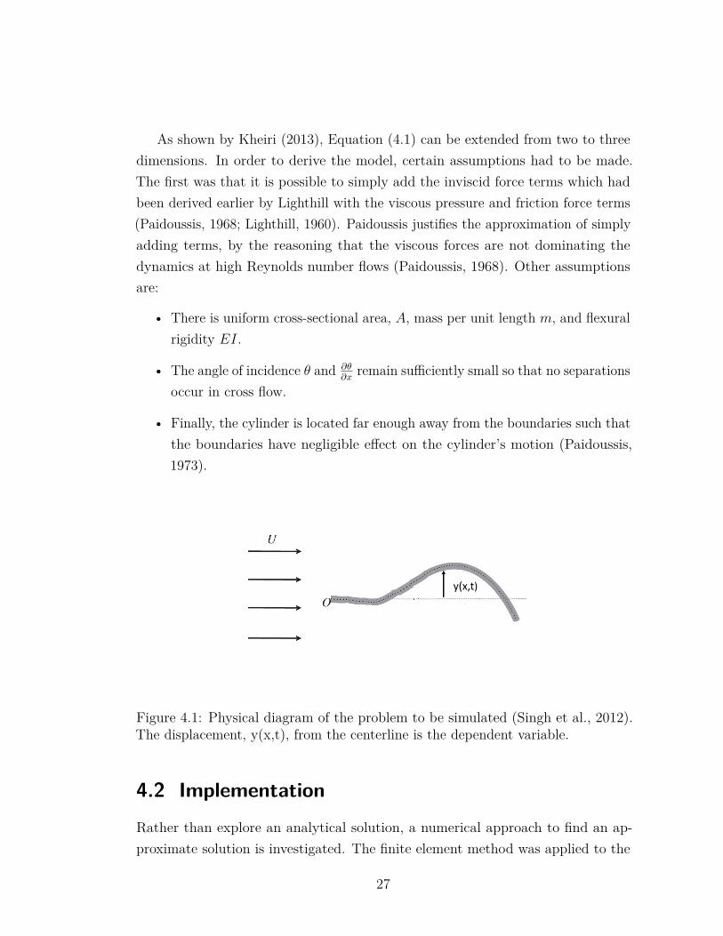
The code was implemented in Deal.ii. The L2 and L∞ errors were computedafter 2,000 time steps with a timestep of dt = 0.001. The number of time stepsand step size was kept constant between the grid refinements. The implementedcode yields the following convergence table for y, w, u, and v. A convergence rateof 2 is found for all variables as expected for Q1 elements. The results are shownin Tables 4.1, 4.2, 4.3, and 4.4. The error in the displacement are shown in Figure4.2 and Figure 4.3 with the correct slop of 2.

Table 4.1: Refinement table for verification of y

cycle # cells # dofs ‖y∗ − yh‖L2 ‖y∗ − yh‖L∞

0 32 132 1.849e-02 - 5.988e-02 -1 64 260 4.603e-03 2.01 1.522e-02 1.982 128 516 1.149e-03 2.00 3.842e-03 1.993 256 1028 2.867e-04 2.00 9.593e-04 2.004 512 2052 7.120e-05 2.01 2.334e-04 2.04

Table 4.2: Refinement table for verification of w

cycle # cells # dofs ‖w∗ − wh‖L2 ‖w∗ − wh‖L∞

0 16 68 6.597e-01 - 1.202e+00 -1 32 132 1.652e-01 2.00 3.152e-01 1.932 64 260 4.135e-02 2.00 7.978e-02 1.983 128 516 1.034e-02 2.00 2.002e-02 1.994 256 1028 2.590e-03 2.00 5.025e-03 1.99

33

Table 4.3: Refinement table for verification of u

cycle # cells # dofs ‖u∗ − uh‖L2 ‖u∗ − uh‖L∞

0 16 68 6.228e+00 - 1.082e+01 -1 32 132 1.573e+00 1.98 2.878e+00 1.912 64 260 3.944e-01 2.00 7.305e-01 1.983 128 516 9.872e-02 2.00 1.834e-01 1.994 256 1028 2.474e-02 2.00 4.599e-02 2.00

Table 4.4: Refinement table for verification of v

cycle # cells # dofs ‖v∗ − vh‖L2 ‖v∗ − vh‖L∞

0 16 68 6.433e-02 - 1.306e-01 -1 32 132 1.570e-02 2.04 3.200e-02 2.032 64 260 3.901e-03 2.01 7.983e-03 2.003 128 516 9.767e-04 2.00 2.003e-03 1.994 256 1028 2.608e-04 1.90 5.875e-04 1.77

34

Figure 4.2: Log-log plot of L2 error for displacement for grid refinement study.Error was calculated after 2,000 timesteps with a step size of 0.001

Figure 4.3: Log-log plot of L∞ error for displacement for grid refinement study.Error was calculated after 2,000 timesteps with a step size of 0.001

35

4.4 Best PracticesIt is important to ensure that a dynamic simulation conserves energy. A simpletest case was used to verify that the energy in the system is being conserved. Thetest case had β = 1, φ = −1, and all other coefficients 0. This corresponds to thewave equation in 1-D. The total energy of the system is equal to the kinetic energyplus the potential energy from stretching the string.

dl dy

dx

x x+dx

y(x+dx)y(x)

Figure 4.4: Close-up of a vibrating string used in the derivation of the energy ofthe system

The formula for the kinetic energy is

Kinetic Energy =∫ L

0

12mv

2dx, (4.23)

where m is the mass per unit length. For this simulation m = 1.The potential energy comes only from the stretching of the string as seen in

Figure 4.4. The change of length of the string over an arbitrary small interval dx isrequired. The length of the string over the interval [x, x+dx] is dl. Assuming smalldeformations, Pythagorean’s theorem can be used to write dl as

dl =√dx2 + dy2 = dx

√√√√1 +(dydx

)2

. (4.24)

36

For small deformations, the square root can be approximated as

dx

√√√√1 +(dydx

)2

≈ dx1 + 1

2

(dydx

)2 . (4.25)

The change in length is then

stretch = new length− old length = dl− dx = 12

(dydx

)2

dx. (4.26)

Energy is force times distance. By assuming constant tension in the string, thepotential energy is then stretch multiplied by tension. For this case, the tension waschosen to be 1. By integrating over the whole length of the string, and substitutingin w = dy

dx the total potential energy can be computed as

Potential Energy =∫ L

0

12w

2dx. (4.27)

By adding the kinetic energy to the potential energy, the total energy of thesystem is

Total Energy = K.E. + P.E =∫ L

0

12mv

2dx +∫ L

0

12w

2dx. (4.28)

The total energy of the system was graphed as a function of time for two differenttime stepping methods. The first was for θ = 1, which corresponds to the implicitbackward-Euler time-stepping scheme. The results are shown in Figure 4.5. It canbe seen from Figure 4.5 that the total energy of the system decays. This is to beexpected for an implicit time-stepping scheme.

37

Figure 4.5: Energy of the system solved using Backward-Euler time-stepping, θ = 1

Next the simulation was performed with θ = 0.5. The kinetic energy, potentialenergy, and total energy were again calculated. As can be seen in Figure 4.6 theenergy for θ = 0.5 is conserved.

Figure 4.6: Energy of the system solved using Crank-Nicholson time-stepping,θ = 0.5

38

Chapter 5 |Model Comparison

5.1 IntroductionIn this chapter, results for the Paidoussis model are compared to results from afull-order model. As explained previously, the reduced order model should be usedto predict stability of set-ups and not specific displacements of the cylinder. If aninstability is formed, the full order model, unlike the reduced-order model, will beable to predict the existence and amplitude of limit cycles.

5.2 Comparison caseThe work of Paidoussis (2002) is followed and in an attempt to recreate hisexperimental results computationally. Therefore, the following parameters are usedfor a cylinder in water.

• D = 1.676 ×10−2 m

• L = 0.330m

• EI = 7.68 ×10−3 Nm2 or E = 1.98 ×106 N/m2

• m = 0.25 kg/m = 1,141 kg/m3

• U ∈ 1,2,4,6 m/s

During these experiments it was recorded by Paidoussis that the dynamics ofthe cylinder were most sensitive to changes in flow velocity. For this reason, flow

39

velocity is the parameter varied. The range for velocity will be between zero andsix meters/second, which is the range that Paidoussis performed his experiments.It has been decided to simulate the cylinder with two different tail pieces. The firstis a cylinder with a blunt downstream end, and the second is a well streamlineddownstream end. These two cases were run at various fluid velocities and thebehaviour of both models are compared in subsequent sections.

For the reduced order model the cylinder must be given an initial displacementor velocity, otherwise the Paidoussis model would return the trivial solution ofzero displacement and zero velocity for all time. This is not the case for the firstprinciples model which can have initial conditions of zero displacement and zerovelocity.

5.2.1 Reduced-Order Model Setup

The reduced order model had an initial displacement of y = x4/24−x3L/6+x2L2/4.This initial displacement was chosen because it satisfies the boundary conditions ofy = 0 and y′ = 0 on the clamped end, x=0, as well as the moment free conditionof y′′ = 0 on the free downstream end, x=L. The simulations were run for 1000timesteps at a timestep of 0.01 seconds. A simulation could usually be completedin about ten minutes.

As previously stated, since a linear model is being used, the displacementof the cylinder either converges to zero or diverges to infinite displacement. Aconvergence to zero represents a stable solution. Divergence is characterized by thetip displacement heading monotonically towards infinity in the reduced order model.Flutter is characterized by a flapping of the tip displacement. Because flutter is aninstability, the amplitude of the oscillations grow exponentially towards infinity.

5.2.2 First Principles Simulation Setup

The full order model had a uniform inlet velocity coming from the left in Figure5.2. The cylinder is clamped on the upstream end and free on the downstreamend. The initial condition for the cylinder is zero displacement and zero velocity.The top and bottom boundaries have slip boundary conditions. The pressure isset to zero for the outlet and the gradient is set to zero for the inlet and for thecylinder-fluid interface. A two-dimensional case was run because the Paidoussis

40

model is a two-dimensional model.The mesh for the full order model consisted of approximately 18,000 hexahedron

cells. Mesh studies were not performed for the full order model. However, Paidoussis’reported experimental data on the instabilities observed for the simulation casesperformed (Paidoussis, 2004). Paidoussis also reported a cylinder tip-displacementof around one to two cylinder diameter lengths (Paidoussis, 2004) for the instabilities.An example of a divergence and flutter instabiltiy from Paidoussis experiments canbe seen in Figure 5.1. Since the full order simulations were within the range observedin Paidoussis’ experiments, it was determined that the meshes were sufficient.

The Reynolds number for the slowest case is 330,000 if the length of the cylinderis used for the characteristic length. This means the simulations are turbulent.However, a turbulence model was not used in the full order simulations. It wasdetermined to be unnecessary to utilize a turbulence model because the full ordersimulations without a turbulence model had instabilities and amplitudes that wereboth in agreement with Paidoussis’ experiments. A turbulence model would havebeen necessary if the precise value of the instability amplitude was of interest. Butthe reduced order model does not predict instability amplitude. Thus, a precisevalue for the instability amplitude is not required to make a comparison betweenthe two models. For this reason, no turbulence model was used during the fullorder simulations.

The time it took for a full order simulation to run was dependent on the velocity.Higher velocity simulations required a smaller timestep to keep the Courant numberdown, and thus resulted in a longer runtime. All simulations were run on a singlecomputer using a quad CPU with 2.83 GHz processor. It took roughly 4 days for asimulation at a velocity of 1 m/s to run. It took about 2 weeks to run a simulationwith a velocity of 6 m/s.

41

Figure 5.1: Pictures from Paidoussis’ experiments for a cylinder in axial flow. Thepicture on the left shows a divergence instability and the picture on the right showsa flutter instability. The center line was drawn in to emphasize the displacementof the cylinder from a neutral position. Both figures show instability amplitudesbetween one and two cylinder diameters. The instability amplitude of the full ordermodel falls within this range.

5.3 Clamped-free with a blunt end comparisonFull order simulations were performed for a cylinder in axial flow with an uncon-strained blunt downstream end. The setup for the simulation is in Figure 5.2. Thereduced order model predicts that this case is stable for all flow speeds tested. Forall speeds simulated, the full order model had a maximum tip displacement of lessthan 1 mm. The displacement for an inlet velocity of four meters per second isshown in Figure 5.4. It is then reasonable to call the cylinder stable which is inagreement with the reduced order model prediction. Although the same solutionwas arrived at for both models, the reduced order model was able to make theseprediction in a matter of minutes as opposed to the full order model that requireddays to run. The grid used for the full order model can bee seen in Figure 5.3.

42

Figure 5.2: Simulation set-up for the the full order model with a blunt downstreamend. The cylinder is clamped on the upstream end and the downstream end isfree. There is also uniform inlet velocity and slip boundary conditions on top andbottom of the channel.

Figure 5.3: The grid used for the first principle simulations with a blunt tailconsisted of approximately 18,000 hexahedron cells.

43

Figure 5.4: Displacement vs time for a blunt end and U= 4 m/s. Similar resultswere obtained for other cases as well.

5.4 Clamped-free with a streamlined end comparisonSimulations were also run for a cylinder with a more streamlined tail. A picture ofthe cylinder shape used in the full order model simulation can be seen in Figure5.5. The number of cells in the full order model simulation is the same as usedin the blunt tail simulations. The f-value in the Paidoussis model is a measure ofhow streamlined the tail section is and ranges from 0 to 1 where f=0 represents aperfectly blunt tail and f=1 represents a perfectly streamlined tail. There is nota precise way of calculating the value of f for a given tail piece. Thus, to directlycompare the two models, it must be done qualitatively. Basic trends can still becompared. The f-value affects the critical velocities that divergence and flutterbegin. It’s noted that the reduced order model used returned the same stabilitypredictions for f values of f=0.6-0.9 for the comparison cases ran. It is reasonableto assume the true f value falls into this range because the tailpiece is fairly wellstreamlined. The grid used by the full order model is shown in Figure 5.6.

44

Figure 5.5: Simulation set-up for the the full order model with a streamlineddownstream end. The cylinder is clamped on the upstream end and the downstreamend is free. There is also uniform inlet velocity.

Figure 5.6: The grid used for the first principle simulations with a streamlined tailconsisted of approximately 18,000 hexahedron cells.

45

5.4.1 U=1

The maximum displacement experienced by the tip in the full order simulation wasapproximately 1 mm after 20 seconds. The reduced order model predicts a stableconfiguration. Although the full order model simulation resulted in the cylinderexperiencing some displacement(see Figure 5.5), it still shows the same conclusionas the reduced order model.

Figure 5.7: Tip displacement (cm) from the full order model for a streamlined tailsetup vs time (s) with U=1 m/s. The figure shows that the configuration can beconsidered stable since the max displacement was roughly only a millimeter after20 seconds.

5.4.2 U=2

As can be seen in Figure 5.8 and Figure 5.9, the full order model simulation isbeginning to show signs of divergence when using an inlet speed of 2 m/s. In thefull order simulation the tip displaces a distance of 1.5 cm and then holds there.The divergence is caused by lift being generated by the streamlined tail piece. Theresults in a force displacing the tip. This is in agreement with the reduced order

46

model which predicts divergence for any f-value between 0.5 and 0.9 with thisconfiguration. It is worth noting again that the reduced order model is unableto predict that the cylinder diverges with an amplitude of 1.5 cm, however it didcorrectly predict that a divergence instability would form. Also Paidoussis doesnot report amplitude of displacement for his experiments but he does mentionfor his experiments there was displacement between 1 to 2 times the cylinderdiameter (Paidoussis, 2004). The simulations had a displacement of around 1.5centimeters which is in agreement with the experimental results of a one to twocylinder diameter displacement. Furthermore, qualitatively the shape is similar tothe divergence experimental result shown in Figure 5.1. This gives us confidencethat our full order simulation is accurate.

Notice that although the simulation was set-up to be symmetrical, round-offerror could be the cause for the cylinder to diverge to a specific side. There arenumerous places where round off could have occurred in the full order model. Onepossibility is in the mesh creation. The node coordinates for the mesh are floatingpoint values which are susceptible to round off error. There could also be round offerror occurring in the solvers. Round-off error could be the cause for the cylinderto initially choose a side to diverge to.

47

Time = 8 s

Time = 10 s

Time = 12 s

Figure 5.8: Results from the full order simulation with a streamlined tail at varioustimes with U=2 m/s shows the cylinder has a divergence instability.

48

Figure 5.9: Tip displacement (cm) from the full order model for a streamlined tailsetup vs time (s) with U=2 m/s. The figure shows the tip displacement having anaverage displacement of roughly 1.5 cm which clearly show a divergence instability.

5.4.3 U=4

The full order model simulation using U=4 m/s still shows divergence as thedominating instability with an average displacement of about 1.2 cm. The shapeof the cylinder can be seen in Figure 5.10. Tip displacement vs time is shown inFigure 5.11. Again, the divergenec is a result of the lift generated by the end piece.Oscillations around the divergence amplitude are greater for U=4 m/s than forU=2 m/s. The oscillations are still small at roughly 0.5 mm, but they show thesystem is beginning to form a flutter instability. Figure 5.12 shows that the reducedorder model predicts that only a divergence instability should form at this speed.Since divergence is still the dominating instability, it is reasonable to say that thefull order model and reduced order model are still in agreement in the instabilityprediction. The divergence amplitude is also still in agreement with Paidoussis’experimental results (Paidoussis, 2004). Again, the choice of instability directioncan be attributed to round-off error.

49

Time = 8 s

Time = 10 s Time = 12 s

Time = 0 s

Figure 5.10: Results from the full order simulation with a streamlined tail at varioustimes with U=4 m/s shows the cylinder forms a divergence instability. This issimilar to the response when U=2 m/s.

50

Figure 5.11: Tip displacement (cm) from the full order model for a streamlinedtail setup vs time (s) with U=4 m/s. The figure shows the tip displacement has adivergence instability but oscillations are starting to grow. This shows that flutteris beginning to form.

Figure 5.12: Tip displacement (cm) from both the full order model and the reducedorder model for a streamlined tail setup vs time (s) with U=4 m/s. The reducedorder model shows the cylinder will diverge by monotonically converging to negativeinfinity

51

5.4.4 U=6

For U=6 m/s, second mode flutter has become the dominating instability in the fullorder model. The cylinder shape for various times is shown in Figure 5.13. Figure5.14 shows the tip displacement as a function of time. Figure 5.16 shows that theflutter is not centered around zero. This provides evidence that the cylinder is alsounstable in the divergence mode as well. The reduced order model predicts flutterat the speed of U=6 m/s. Of course, as has been previously been pointed out, thefull order model is able to predict the amplitude of each instability.

Figure 5.13: Results from the full order simulation with a streamlined tail at varioustimes with U=6 m/s shows the cylinder has a flutter instability.

52

Figure 5.14: Tip displacement (cm) from the full order model for a streamlinedtail setup vs time (s) with U=6 m/s. The figure shows a divergence instabilityforms first but flutter oscillations are starting to grow. The oscillations appear tobe centered around the divergence average displacement of 0.8 cm.

Figure 5.15: Tip displacement (cm) from both the full order model and the reducedorder model for a streamlined tail setup vs time (s) with U=4 m/s. The reducedorder model shows the cylinder will flutter by the amplitude of the tip displacementdiverging non-monotonically

53

There was again good agreement between the reduced order model, the full-order model, and experiments for a streamlined tail. In the reduced order modelflutter forms abruptly, but the full order model shows flutter slowly forming fromdivergence. The general trends are still in agreement because both models predictthat first divergence develops and then becomes flutter at higher speeds. This isalso in accordance with experimental observations by Paidoussis (Paidoussis, 2004).The major differences between the models is that the full-order model is able topredict amplitude of the instabilities and the reduced order model is only ableto predict the existence of an instability. After performing the simulations, thefollowing conclusions can be drawn:

• There is agreement between reduced order model and the full order modelon the instability type for both the blunt end and the streamlined end. Theresults are summarized in Table 5.1.

• Cylinders with blunt tails are more stable than cylinders with streamlinedtails.

• The reduced order model is able to accurately predict if and which instabilitythe cylinder would experience. The reduced order model cannot predictthe existence of limit cycles because it is a linear model. Therefore, if theamplitude of the instability is of interest to the researcher then the full ordermodel is required.

• When the reduced order model predicts the cylinder is stable, it is unnecessaryto run the full order model because they will both return results of near zerodisplacement.

• The time required to perform a reduced order simulation is orders of magnitudefaster than the full order model used herein.

54

Figure 5.16: Tip displacement (cm) from the full order model for a streamlined tailsetup vs time (s) with U=1,2,4,6 m/s.

Table 5.1: A recap of the results of all the comparison cases performed.

Blunt end Streamlined endExperiment ROM FOM Experiment ROM FOM

1 m/s Stable Stable Stable Stable Stable Stable2 m/s Stable Stable Stable Diverge Diverge Diverge4 m/s Stable Stable Stable Diverge Diverge Diverge6 m/s Stable Stable Stable Flutter Flutter Flutter

55

Chapter 6 |Conclusions

6.1 Summary of Work PerformedIn this thesis two different models for a cylinder in axial flow were compared. Thefirst was the Paidoussis model. It required formulating the governing equationinto weak form and then implementing into a custom finite element program. Thecomputer program written to solve the Paidoussis equation was written using theopen source finite element library deal.ii, and was rigorously verified by usingthe method of manufactured solutions. This model coupled the incompressibleNavier-Stokes equations for the fluid with an elastic model for the solid. The secondmodel was implemented using OpenFOAM for the fluid domain and an in-housefinite element solver called FEANL for the solid. These were coupled using anin-house coupling algorithm. The contribution of this work was to provide furtherevidence for the Paidoussis model to predict instability of elastic cylinders in axialflow.

This thesis highlights the strengths and weaknesses of both modeling approaches.The strength of the Paidoussis model is that it is a linear differential equation.This allows it to be implemented and run very quickly. This gives it the abilityto quickly return results on predictions of instabilities. However, the Paidoussisstrength is also its weakness. By being a linear equation, the Paidoussis model isnot able to predict non-linear effects such as limit cycles.

On the other hand, the ability to predict non-linear phenomenon such as limit-cycle amplitude is one of the strengths of the full order model. The price of usingthese non-linear equations is a significantly higher cost in computational resources.

56

This is due to non-linear equations being much more difficult to solve. A recap ofthe work completed in this thesis is provided below.

1. A finite element program to solve the Paidoussis equation.

2. The method of manufactured solutions was used to verify the correct imple-mentation of the reduced order model.

3. The energy of the system for the Paidoussis model was calculated for twodifferent time stepping schemes.

4. Simulations of a cylinder in axial flow using a full order solver were performed.

5. The stability predictions of both models were compared.

6.2 Future WorkThere is more than one way to create a reduced-order model. In this thesis, thereduced-order model made assumptions about the physics being modelled. Theseassumptions were then used to make simplifications to the governing equationsand reduce them down to a linear equation. But this comes at a price; makingassumptions can lead to losing the effects of important physics, and brings intoquestion the validity of the assumptions being made.

Another approach to creating a reduced-order model (ROM) is by takingsnapshots of the solution from the full-order model. A statistical method is thenapplied to the set of snapshots to derive a basis for the system’s response that is"optimal" in some sense. By perturbing the conditions used to create the ROM, itcan be used to simulate different conditions.

This statistical or empirical approach to ROM creation has the advantage ofbeing devised from first principles. It can be thought of as being a method formathematically choosing which physics are to be left out of the model. The majoradvantage of using an empirical reduced order model is that they still retain of thenon-linearity of the original governing equations. This captures some non-lineareffects such as limit cycles. This is in contrast to making educated guesses onwhat assumptions to make so that the governing equations can be simplified. Bothmethods have their strengths and weakness. Empirical ROMs are typically more

57

accurate but take longer to run and have smaller ranges of validity. Reduced-ordermodels devised by making assumptions of the underlying physics, might not offerthe same accuracy of the empirical ROM but can often be computed faster. To theauthor’s knowledge no towed array empirical ROMs exist.

One problem with empirical ROMs is that they are very specific to the conditionsused to create them; i.e. the domain, flow conditions etc. This leads to ROMsunable to handle large deformations because of change to the domain. Unfortunately,towed arrays can have large deformations and it would be prohibitively expensiveto produce a ROM for all the possible configurations the array can deform into.

I propose overcoming this deficiency by using a combination of domain decompo-sition and proper orthogonal decomposition to create a database of “ROM Elements”that can be assembled and coupled into complicated configurations. By dynamicallyupdating the elements as the structure deforms, I hope to be able to handle largedeformations in fluid-structure interaction problems. My idea is similar to thefinite element method. Finite elements decompose the domain into a number ofelements where the governing equations are solved for each element. This techniquewill be similar in that the domain will be broken up into elements, but the shapefunction for the element will be a velocity field throughout the domain. In essence,it’s creating a very large set of reduced order models by assembling reduced ordermodels from a much smaller set of generator reduced-order models. By utilizing amuch smaller generator set, the computation and memory requirements should besignificantly reduced. To keep the generator set small, the simple geometry of atowed array will utilized.

I plan on applying this technique to model a cylinder in axial flow. To the bestof my knowledge, all reduced-order modelling techniques for a cylinder in axialflow have consisted of making assumptions on the physics. There have been noattempts to apply a statistical approach to creating a reduced-order model for acylinder in axial flow.

58

Appendix A|Non Technical Abstract

Computer simulations are playing an increasingly important role in the designprocess for engineers. This has lead to a demand to be able to simulate complexsystems with a high level of accuracy. Advances in computer hardware has greatlyincreased our computational abilities over the years. Problems that used to be toocomputationally expensive can now be routinely solved by simply applying a lot ofcomputing power.

The successful application of computer simulation to engineering has resulted ina demand for accurate solutions at a fraction of the time. To answer that problem,researchers have developed reduced order models by making assumptions on whichphysics of the problem are dominating. The assumptions, simplify the governingequations the computer has to solve, and results in simulations that run orders ofmagnitude faster. The computational savings come at a price. The price being thatthe reduced order model does not capture all the physics of the problem. Therefore,it is of absolute importance to know under what situations the unmodeled physicshave little effect so that a reduced order model can be used to gain a computationalsavings.

This thesis focuses on comparing a first-principles fluid-structure interactionsolver and a reduced order model. A fluid-structure interaction problem was chosenbecause of the high computational cost that is associated with that type of multi-physics problem. The full order model solves the incompressible Navier-Stokesequations for the fluid and elasticity equations for the solid. The reduced order

59

model chosen for comparison in the thesis is the Paidoussis model for a cylinder inaxial flow. The free stream velocity was varied for a cylinder with a blunt tail andfor a streamlined tail. The results were then compared to the predictions by thefull order solver.

60

Bibliography

C. Ablow and S. Schechter. Numerical simulation of undersea cable dynamics.Ocean Engineering, 10(6):443 – 457, 1983.

W. Bangerth, T. Heister, L. Heltai, G. Kanschat, M. Kronbichler, M. Maier,B. Turcksin, and T. D. Young. The deal.ii library, version 8.1. 1:1, 2013.

A. Barbagelata, P. Guerini, and L. Troiana. Thirty years of towed arrays at NURC.Oceanography, 21, No2:24–33, 2008.

Y. Bazilevs, V. Calo, T. Hughes, and Y. Zhang. Isogeometric fluid-structureinteraction: theory, algorithms, and computations. Computational Mechanics, 43(1):3–37, 2008.

Y. Bazilevs, M.-C. Hsu, J. Kiendl, R. Wüchner, and K.-U. Bletzinger. 3d simulationof wind turbine rotors at full scale. part ii: Fluid–structure interaction modelingwith composite blades. International Journal for Numerical Methods in Fluids,65(1-3):236–253, 2011. ISSN 1097-0363.

S. Bhattacharyya, C. Vendhan, and K. Sudarsan. The finite element method forhydroelastic instability of underwater towed cylindrical structures. Journal ofSound and Vibration, 237(1):119 – 143, 2000. ISSN 0022-460X.

R. D. Blevins. Applied Fluid Dynamics Handbook. Van Nostrand Reinhold Company,1984.

S. C. Brenner and L. R. Scott. The Mathematical Theory of Finite Element Methods.Spring, 2002.

D. Calkins. A metamodel-based towed system simulation. Ocean Engineering, 26(11):1183 – 1247, 1999. ISSN 0029-8018.

R. L. Campbell and E. G. Paterson. Fluid–structure interaction analysis of flexibleturbomachinery. Journal of Fluids and Structures, 27(8):1376–1391, 2011.

R. H. C.C. Ni. An experimental study of the flow-induced motions of a flexiblecylinder in axial flow. Journal of Fluids Engineering, 100:389–394, 1978.

61

D. Chapman. Towed cable behaviour during ship turning manoeuvers. OceanEngineering, 11(4):327 – 361, 1984. ISSN 0029-8018.

Y. Chen and M. Weber. Flow-induced vibrations in tube bundle heat exchangerswith cross and parallel flow. In ASME Symposium on Flow Induced Vibrationsin Heat Exchangers, ed., DD Reiff, pages 57–77, 1970.

E. De Langre, M. P. Paidoussis, O. Doare, and Y. Modarres-Sadeghi. Flutter oflong flexible cylinders in axial flow. Journal of Fluid Mechanics, 571:371–389, 02007. ISSN 1469-7645.

J. Donea, S. Giuliani, and J.-P. Halleux. An arbitrary lagrangian-eulerian finiteelement method for transient dynamic fluid-structure interactions. ComputerMethods in Applied Mechanics and Engineering, 1982. ISSN 0045-7825.

A. P. Dowling. The dynamics of towed flexible cylinders part 1. neutrally buoyantelements. Journal of Fluid Mechanics, 187:507–532, 1 1988. ISSN 1469-7645.

K. Dumont, J. Vierendeels, R. Kaminsky, G. Van Nooten, P. Verdonck, andD. Bluestein. Comparison of the hemodynamic and thrombogenic performanceof two bileaflet mechanical heart valves using a cfd/fsi model. Journal of biome-chanical engineering, 129(4):558–565, 2007.

J. Gagnon and M. Paidoussis. Fluid coupling characteristics and vibration ofcylinder cluster in axial flow. part ii: Experiments. Journal of Fluids andStructures, 8(3):293 – 324, 1994a. ISSN 0889-9746.

J. Gagnon and M. Paidoussis. Fluid coupling characteristics and vibration ofcylinder cluster in axial flow. part i: Theory. Journal of Fluids and Structures, 8(3):257 – 291, 1994b. ISSN 0889-9746.

P. Gerstoft, W. S. Hodgkiss, W. Kuperman, H. Song, M. Siderius, and P. L. Nielsen.Adaptive beamforming of a towed array during a turn. Oceanic Engineering,IEEE Journal of, 28(1):44–54, 2003.

J. Gobat and M. Grosenbaugh. Whoi cable: time domain numerical modelingof moored and towed oceanographic systems. In OCEANS ’98 ConferenceProceedings, volume 3, pages 1681–1685 vol.3, 1998.

J. Gobat and M. Grosenbaugh. Time-domain numerical simulation of ocean cablestructures. Ocean Engineering, 33(10):1373 – 1400, 2006. ISSN 0029-8018.

K. Gogan. The sounds of the sea: Marione acoustics, April 2014.

M. A. Grosenbaugh. Transient behavior of towed cable systems during ship turningmaneuvers. Ocean Engineering, 34(11-12):1532 – 1542, 2007. ISSN 0029-8018.

62

C. C. G.S. Traintafyllou. The dynamics of towed arrays. Offshore Mech. Arct. Eng,111:6, 1989.

W. R. Hawthorne. The early development of the dracone flexible barge. Proceedingsof the Institution of Mechanical Engineers, 175(1):52–83, 1961.

S. Hopland. Investigation of cable behaviour in water during laying of fiberopticsubmarine cables. In Proc. International Wire and Cable Symposium, pages734–39, 1993.

R. Issa. Solution of the implicitly discretized fluid flow equations by operatorsplitting. Journal of Computational Physics, 62:6, 1989.

H. Jasak. Error analysis and estimation for the finite volume method with applica-tions to fluid flows. PhD thesis, Imperial College London (University of London),1996.

A. O. Katsuhisa Fujita. Effect of structural dimensions on dynamic stability ofelastic beam subject to axial flow in confined narrow passage. System Designand Dynamics, 4:809–822, 2010.

M. Kheiri, M. Païdoussis, M. Amabili, and B. Epureanu. Three-dimensionaldynamics of long pipes towed underwater. part 1: The equations of motion.Ocean Engineering, 00(0):0– 0, 2013. ISSN 0029-8018.

C. Kopp. Identification underwater with towed array sonar. In Pacifici MaritimeConference, 2010.

U. Kuttler, C. Forster, and W. A. Wall. A solution for the incompressibility dilemmain partitioned fluid–structure interaction with pure dirichlet fluid domains. Com-putational Mechanics, 38(4-5):417–429, 2006.

M. Lasky, R. Doolittle, B. Simmons, and S. Lemon. Recent progress in towedhydrophone array research. Oceanic Engineering, IEEE Journal of, 29(2):374 –387, april 2004. ISSN 0364-9059.

S. G. Lemon. Towed-array history, 1917-2003. IEEE Journal of Oceanic Engineering,29:365–373, 2004.

M. J. Lighthill. Note on the swimming of slender fish. Journal of Fluid Mechanics,9:305–317, 9 1960. ISSN 1469-7645.

Z. Liu, Y. Liu, and J. Lu. Fluid-structure interaction of single flexible cylinder inaxial flow. Computers & Fluids, 56(0):143 – 151, 2012. ISSN 0045-7930.

63

F. Lu, E. Milios, S. Stergiopoulos, and A. Dhanantwari. New towed-array shape-estimation scheme for real-time sonar systems. Oceanic Engineering, IEEEJournal of, 28(3):552 – 563, july 2003. ISSN 0364-9059.

A. Masud and T. J. Hughes. A space-time galerkin/least-squares finite elementformulation of the navier-stokes equations for moving domain problems. ComputerMethods in Applied Mechanics and Engineering, 146(1):91–126, 1997.

H. G. Matthies and J. Steindorf. Partitioned strong coupling algorithms for fluid–structure interaction. Computers & Structures, 81(8):805–812, 2003.

C. Michler, S. Hulshoff, E. Van Brummelen, and R. De Borst. A monolithicapproach to fluid–structure interaction. Computers & fluids, 33(5):839–848, 2004.

F. Milinazzo, M. Wilkie, and S. Latchman. An efficient algorithm for simulatingthe dynamics of towed cable systems. Ocean Engineering, 14(6):513 – 526, 1987.ISSN 0029-8018.

S. T. Miller, R. Campbell, C. Elsworth, J. Pitt, and D. Boger. An overset gridmethod for fluid-structure interaction. World Journal of Mechanics, 2014, 2014.

M. Obligado and M. Bourgoin. An experimental investigation of the equilibriumand stability of long towed cable systems. New Journal of Physics, 15(4):043019,2013.

Orcina. Orcaflex manual version 9.8a.

M. Païdoussis. Dynamics of submerged towed cylinders. McGill University, Me-chanical Engineering Research Laboratories, 1970.

M. Paidoussis. Dynamics of cylindrical structures subjected to axial flow. Journalof Sound and Vibration, 29(3):365 – 385, 1973.

M. P. Paidoussis. Stability of towed, totally submerged flexible cylinders. Journalof Fluid Mechanics, 34:273–297, 10 1968.

M. P. Paidoussis. Fluid-Structure Interactions Slender Structures and Axial FlowVolume 2. Elsevier Academic Press, 2004.

H. Park, D. Jung, and W. Koterayama. A numerical and experimental study ondynamics of a towed low tension cable. Applied Ocean Research, 25(5):289 – 299,2003.

J. Pike. Towed array. http://www.globalsecurity.org, March 2013.

64

J. Potter, E. Delaory, S. Constantin, and S. Badiu. The a lightweight, ultra-thin (8mm od) towed array for use from small vessels of opportunity. In UnderwaterTechnology, 2000. UT 00. Proceedings of the 2000 International Symposium on,pages 49 –53, 2000.

P. Roache. Verification and Validation in Computational Science and Engineering.Hermosa Publishers, 1998.

K. Singh, S. Michelin, and E. De Langre. The effect of non-uniform damping onflutter in axial flow and energy-harvesting strategies. Proceedings of the RoyalSociety A: Mathematical, Physical and Engineering Science, 468(2147):3620–3635,2012.

S. Srivastava and C. Ganapathy. Experimental investigations on loop manoeuvre ofunderwater towed cable-array system. Ocean Engineering, 25(1):85 – 102, 1998.

S. Turek and J. Hron. Proposal for numerical benchmarking of fluid-structureinteraction between an elastic object and laminar incompressible flow. In H.-J. Bungartz and M. Schäfer, editors, Fluid-Structure Interaction, volume 53of Lecture Notes in Computational Science and Engineering, pages 371–385.Springer Berlin Heidelberg, 2006. ISBN 978-3-540-34595-4.

M. Vaz and M. Patel. Transient behaviour of towed marine cables in two dimensions.Applied Ocean Research, 17(3):143 – 153, 1995. ISSN 0141-1187.

M. T. Vineet Kumar Srivastava, YVSS Sanyasiraju. Dynamic behavior of underwa-ter towed-cable in linear profile. International Journal of Scientific & EngineeringResearc, 2:9, July 2011.

M. Zhdanov. 3D inversion of towed streamer EM data: A model study of theHarding field and comparison to 3D CSEM inversion, SEG Exhibition, September2011.

65