a comparison of methods used in flood-frequency … · a comparison of methods used in...
TRANSCRIPT
A Comparison of Methods Used In Flood-Frequency Studies for Coastal Basins in California
GEOLOGICAL SURVEY WATER-SUPPLY PAPER 1580-E
Prepared in cooperation with the California Department of ff^ater Resources
A Comparison of Methods Used In Flood-Frequency Studies for Coastal Basins in CaliforniaBy R. W. CRUFF and S. E. RANTZ
FLOOD HYDROLOGY
GEOLOGICAL SURVEY WATER-SUPPLY PAPER 1580-E
Prepared in cooperation with the California Department of Heater Resources
JNITED STATES GOVERNMENT PRINTING OFFICE, WASHINGTON : 1965

UNITED STATES DEPARTMENT OF THE INTERIOR
STEWART L. UDALL, Secretary
GEOLOGICAL SURVEY
Thomas B. Nolan, Director
For sale by the Superintendent of Documents, U.S. Government Printing Office Washington, D.C. 20402 - Price 70 cents (paper cover)
CONTENTS
Page
Abstract______________________.__-_--_____---___---__ ElIntroduction_.____________________________________________________ 1
Purpose and scope-----_----_-___-__-_-_---___--____----__----_ 3Acknowledgments ____-__-__-_-_-_____----________-___-___-____ 3Statistical equations used in this study___________________________ 5
Description of the methods of analysis used in this study_______________ 5Index-flood method.___________________________________________ 6Multiple correlation_________________________________________ 9Logarithmic normal distribution____-____-_____-_-_-___-____-_-_- 10Extreme-value probability distribution or Gumbel method________ 12Pearson type III distribution_________________________-_________ 13Gamma distribution.__________________________________________ 14
Analysis of flood frequency in the San Diego area._____________________ 17Index-flood method.___________________________________________ 17Multiple correlation_________________________________________ 21Logarithmic normal distribution_________----_---_____-_-_-_____- 22Extreme-value probability distribution or Gumbel method. __ _______ 25Pearson type III distribution.__________--____-____-_--_-_-_-_-- 28Gamma distribution.____-________________._-_-__-__-_-_____-_- 28
Analysis of flood frequency in north coastal California ______________ 29Index-flood method.__________________________---_-__-----_--__ 33Multiple correlation__________________________________________ 41Logarithmic normal distribution__________-____---_____-________- 41Extreme-value probability distribution or Gumbel method__________ 43Pearson type III distribution.__________________________________ 45Gamma distribution.__________________________________________ 45
Discussion of results of the analyses_______________________________ 47Index-flood and multiple-correlation methods.____________________ 51Statistical distributions.___-_-___-----__-----_--_-_-__-----__--_ 51
Summary and conclusions__________________________----_-_-__--__ 54References cited_____-______-_-_____-_____________---_-----_----- 56
m

IV CONTENTS
ILLUSTRATIONS
[All plates are in pocket]
PLATE 1. Map of San Diego area showing location of stream-gagingstations used in this study.
2. Map of north coastal California showing stream-gaging stations and boundaries of hydrologic regions used in this study.
Page FIGURE 1. Index map of California_-______--__----_---__----_-_ El
2. Graph showing relation of C in the gamma distributionto log (M/M0)___-___-______--___---__-_----_-___ 16
3. Bar graph showing period of peak-discharge record forgaging stations in the San Diego area.______________ 19
4. Flood-frequency curve for Santa Ysabel Creek at Suther land Dam__________________________ 20
5. Dimensionless regional flood-frequency curve for the SanDiego area (index-flood method)__________________ 21
6-8. Graph showing relation of 6. Mean annual flood to drainage area in the San Diego
area (index-flood method)__-___--_-----_---___- 227. Mean and standard deviation of logarithms of
annual peak discharges to drainage area in the San Diego area._ _______-_---__-_--_----_----__- 26
8. Mean and standard deviation of annual peak dis charges to drainage area in the San Diego area___ 27
9. Bar graph showing period of peak-discharge record forgaging-stations in north coastal California ___________ 31
10. Flood-frequency curve for Klamath River at Klamath__ 3311. Flood-frequency curve for Eel River at Scotia__________ 3412. Dimensionless regional flood-frequency curves for north
coastal California (index-flood method)______________ 3513-18. Graph showing relation of
13. Mean annual flood to drainage area in the CoastRanges (index-flood method).________________ 37
14. C to mean annual basinwide precipitation in theKlamath Mountains (index-flood method) _____ 38
15. The mean of the logarithms of annual peak dis charges to drainage area in the Coast Ranges___ 42
16. The standard deviation of the logarithms of annual peak discharges to mean annual basinwide pre cipitation in the Klamath Mountains.._______ 44
17. The mean and the standard deviation of annual peakdischarges to drainage area in the Coast Ranges. _ 44
18. C to mean annual basinwide precipitation in theKlamath Mountains (gamma distribution) _____ 46

CONTENTS
TABLES
Page TABLE 1. Pearson type III recurrence curve data, Kgt values, in standard
deviations from the mean_______________________________ E152. Summary of hydrologic parameters for basins in the San Diego
area--__---_---___-_-_-____-__-___-_-_-_-________-____ 183. Qsa for streams in the San Diego area as determined from
graphically derived flood-frequency curves and by various methods of regional flood-frequency analysis._____________ 23
4. Qioo for streams in the San Diego area as determined from graphically derived flood-frequency curves and by various methods of regional flood-frequency analysis_-_-__-_______ 24
5. Summary of pertinent hydrologic parameters for basins innorth coastal California______-____________-____________ 32
6. Qso for streams in north coastal California as determined from graphically derived flood-frequency curves and by various methods of regional flood-frequency analysis.------------- 39
7. Qioo for streams in north coastal California as determined from graphically derived flood-frequency curves and by various methods of regional flood-frequency analysis.-..---------- 40
8. Summary of differences between discharges determined from graphically derived flood-frequency curves and discharges computed by various methods of regional flood-frequency analysis. ______________________________________________ 48
9. Summary of differences between Qso determined from graphically- derived flood-frequency curves and Q50 computed from various distributions using statistical parameters from individual station arrays.________________________________________ 54


FLOOD HYDROLOGY
A COMPARISON OF METHODS USED IN FLOOD- FREQUENCY STUDIES FOR COASTAL BASINS
IN CALIFORNIA
By K. W. GRUFF and S. E. KANTZ
ABSTRACT
This study compares the results of regional flood-frequency studies made by several methods and appraises the relative reliability of these methods. The areas selected for study were the subhumid San Diego area in southwestern California and the humid coastal area in northwestern California. The follow ing six methods of analysis were applied to each region: Index-flood method, multiple correlation, logarithmic normal distribution, extreme-value probability distribution (Gumbel method), Pearson type III distribution, and gamma distri bution. The last four methods named involved not only the computation of the statistics appropriate to the distributions, but also the relating of these statistics to basin and climatologic characteristics. On the basis1 of an empirical, non- statistical test, the following conclusions were reached :
1. All methods of analysis give better results in a humid region than in a sub- humid region because streamflow is less variable in a humid region.
2. If historical data, either qualitative or quantitative, are available concerning the magnitude of floods that occurred in the years prior to the collection of streamflow records, the multiple-correlation method of analysis is preferred. Only this method and the index-flood method benefit from the historical data, which, in effect, extend the time base of the analysis. The multiple-correlation method is superior to the index-flood method be cause it has a far more rational basis and in addition gives better results.
3. Where the peak-discharge data are limited entirely to the period during which streamflow records were collected (no historical data available), a method based on the distribution of the array of peak flows is preferred because of its greater objectivity. Of the four distributions tested, the Pearson type III is the most desirable. It is more flexible than the other three and will generally fit the peak-discharge data best.
Although this comparison study of flood-frequency methods was based on small samples from only one part of the United States, the results and con clusions appear to be meaningful because they can be explained rationally.
INTRODUCTION
The principle of analyzing flood magnitudes on a probability basis is almost universally accepted because its use permits economic con siderations, as well as hydrologic factors, to govern the planning and
El

E2 FLOOD HYDROLOGY
design of projects that are susceptible to flood damage. There is no universal acceptance, however, of any single method of making the flood-frequency analysis. Usually, a basic objective of the analysis is to derive flood magnitude-frequency relations which may be used at a site for estimating the magnitude of rare or unusual flood events, such as the peak discharge that has an average probability of being exceeded only once in 100 years (Qwo ) or of being exceeded only once in 50 years (Q50 ). Because our records of flood discharges are gen erally short less than 30 years, on the average extrapolation by some means is required to estimate the magnitudes of unusual floods. How ever, the magnitudes so determined depend, to a large degree, on the method of frequency analysis that governed the extrapolation. Therefore, it is not unusual for independent workers, using the same short streamflow records but different methods of analysis, to obtain widely differing values of discharge corresponding to Q50 or $100- Furthermore, because of the element of uncertainty that characterizes any extrapolation, it is seldom possible to decide which of the derived discharges are the most accurate or which method of analysis is the most reliable.
For a detailed discussion of the many methods of deriving flood magnitude-frequency relations, the reader is referred to reports by Jarvis and others (1936) and Benson (1962). Several of the meth ods described in those reports are no longer in favor, and others have had varying degrees of popular acceptance over the years. At present (1964), the methods most commonly used in this country are the four listed below. The agency or agencies shown in parentheses are the chief proponents of the methods.
1. Index-flood method (U.S. Geol. Survey).2. Multiple-correlation (U.S. Bur. of Public Roads and U.S. Geol.
Survey).3. Logarithmic normal distribution (U.S. Army, Corps of Engineers).4. Extreme-value probability distribution or Gumbel method (U.S.
Weather Bur.).These four methods and two additional ones the Pearson type III
distribution and the gamma distribution were used in this study. The Pearson type III distribution was included because the authors feel that this method is likely to regain the popularity it once had in probability studies of peak discharge. The gamma distribution was included because it is increasingly being used, both in the United States and abroad, for studying the probability of occurrence of hy- drologic events, including peak discharges.

METHODS USED IN FLOOD-FREQUENCY STUDIES, CALIFORNIA E3
PURPOSE AND SCOPE
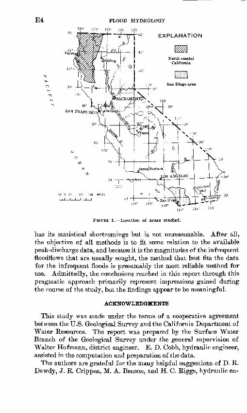
The purpose of this study was to compare the results obtained by applying each of the six methods of flood-frequency analysis to identi cal sets of peak-discharge data. Specifically, it was the values of Q50 and (? 100 , computed by each method, that were compared. One com parison was made for streams in the San Diego area in south coastal California, and another was made for streams in north coastal Cali fornia. (See fig. 1.) There were several reasons for selecting these two areas. First, the comparison is given broader scope by using two areas that differ greatly in the amount of precipitation they receive; the San Diego area is subhumid, whereas the north coastal area is very humid. Second, flood-frequency studies have recently been published for each area, and the hydrologic factors needed in the analyses were therefore readily available. The San Diego area study, published by the California Department of Water Resources (1963), analyzed the data for 18 stream-gaging stations by two methods the index-flood method and multiple correlation. Of the 18 peak-discharge records, 2 were longer than 35 years, 11 were between 20 and 35 years, and 5 were shorter than 20 years. The study for north coastal California published by the U.S. Geological Survey (Rantz, 1964) analyzed the data for 27 stream-gaging stations by the index-flood method. Of the 27 peak-discharge records, 4 were longer than 30 years, 9 were between 10 and 30 years, and 14 were shorter than 10 years.
The principal reason for selecting the two areas lay in the fact that, although the discharge records for the streams were relatively short, the magnitudes of the greatest and second greatest flood peaks in the past 100 years were generally known within reasonable limits of accuracy. With this knowledge it was possible to appraise the results obtained by each of the six methods of analysis and to draw conclusions concerning the relative reliability of the methods.
Many competent statisticians, using long-term discharge records and rigorous statistical treatment, have made comparison studies of the various methods of analyzing flood magnitude-frequency relations without arriving at definitive conclusions concerning the superiority of any one method. Hence the plethora of methods of analysis from which the practicing engineer must choose before making a flood- frequency study. In view of the many uncertainties involved in a comparison study of methods of analysis, the authors have eschewed any rigorous statistical approach, such as an analysis of variance or a determination of confidence limits. They have adopted, instead, a simple pragmatic approach in which the basis of comparison is the relative ability of the various methods to reproduce Q50 and Qi0o at each of the study sites in the two California areas. This approach
770-401 O J©5 2
E4 FLOOD HYDROLOGY
124° 123" 122° 121" 120"
EXPLANATION
117° H6°
FIGURE 1. Location of areas studied.
has its statistical shortcomings but is not unreasonable. After all, the objective of all methods is to fit some relation to the available peak-discharge data, and because it is the magnitudes of the infrequent floodflows that are usually sought, the method that best fits the data for the infrequent floods is presumably the most reliable method for use. Admittedly, the conclusions reached in this report through this pragmatic approach primarily represent impressions gained during the course of the study, but the findings appear to be meaningful.
ACKNOWLEDGMENTS
This study was made under the terms of a cooperative agreement between the U.S. Geological Survey and the California Department of Water Resources. The report was prepared by the Surface Water Branch of the Geological Survey under the general supervision of Walter Hofmann, district engineer. E. D. Cobb, hydraulic engineer, assisted in the computation and preparation of the data.
The authors are grateful for the many helpful suggestions of D. R. Dawdy, J. R. Crippen, M. A. Benson, and H. C. Riggs, hydraulic en-

METHODS USED IN FLOOD-FREQUENCY STUDIES, CALIFORNIA E5
gineers of the Geological Survey, who reviewed the manuscript. How ever, the subject treated here is not one on which unanimity of opinion can be expected. The opinions and assertions in this report are those of the authors and do not, in all particulars, reflect the views of their coworkers in the Geological Survey.
STATISTICAL EQUATIONS USED IN THIS STUDY
We assume that the reader has some knowledge of elementary statistics and is familiar with common statistical nomenclature and with the equations for computing such elemental items as mean, stand ard deviation, correlation coefficient, and linear regression equation. These terms and equations can be found in any standard statistics text (for example, Ezekiel and Fox, 1959). All other statistical equations that are used in this report are explained where they first appear and are thereafter referred to by number as equation 1, equation 2, and so on.
DESCRIPTION OF THE METHODS OF ANALYSIS USED INTHIS STUDY
In this section of the report, the six methods of analysis used in this study are briefly described. In all six methods the streamflow data analyzed consist of the momentary maximum discharge of each year of record. Gaging stations whose peak discharges are seriously affected by manmade storage or diversion are not used. All six methods attempt to make the most efficient use of the data available. The index-flood and multiple-correlation methods are to some extent empirical because the graphical curve-fitting procedures that are basic to both methods require a certain amount of subjectivity on the part of the analyst. These methods have the advantage of permitting the analyst to use whatever qualitative or historical information is avail able for extrapolating the flood-frequency relation. The other four methods are empirical in the sense that a type of distribution loga rithmic normal, extreme-value probability, Pearson type III, or gamma is arbitrarily selected for use. One may theorize concerning the probability distribution that describes the occurrence of flood events, but the lack of agreement among hydrologists indicates that the "true" distribution is not known. Once a distribution is selected for use, however, the analysis becomes strictly objective, and the ex trapolation is automatically made from a mathematical determination of the statistics mean, standard deviation, and coefficient of skew of the station data. Qualitative or historical data cannot be assessed, however, when a rigorous statistical solution is made. On occasion, this type of information is used to define or modify the high-water end

E6 FLOOD HYDROLOGY
of the computed flood-frequency relation; but when this information is so used, the statistical distribution no longer controls the all-impor tant high-water end of the flood-frequency relation. As in the empiri cal index-flood and multiple-correlation methods, the results obtained will depend to a large degree on the judgment of the analyst in inter preting the historical information and assigning probabilities to the peak discharges. In this report, an objective mathematical treatment was used for the four methods involving standard statistical distribu tions, with no consideration given to qualitative or historical information.
Regardless of the method of analysis used, it is customary to develop flood magnitude-frequency relations that are applicable to an entire region rather than to a single gaging station. Because the flood series for a single station is a short random sample, it may not be representa tive of the long-term distribution of flood events at the gaging station. Combining records for all stations in a hydrologically homogenous area tends to reduce the sampling error associated with a nonrepresent- ative sample. Another advantage of the regional flood-frequency relation is that it can be applied to ungaged sites in the region. The boundaries of a homogeneous region must be rationally delineated from a knowledge of the hydrology of the region; commonly, these bound aries will coincide with the boundaries of physiographic sections de lineated by Fenneman (1931, 1938) or with the boundaries of regions delineated on soil classification maps published by the U.S. Soil Con servation Service. In making a regional study, a common base period of years is usually used for each gaging station. This base period is generally the period of record for the older gaging stations in the re gion, and the shorter records are extended by correlation procedures to cover the base period.
Generally, the term "regionalization," as used by engineers engaged in flood-frequency analysis, refers not only to the delineation of the boundaries of hydrologically homogeneous regions, but also to the establishment of relations between pertinent characteristics of the flood-frequency curve and basin or climatologic parameters within the homogeneous region. For example, values of the mean annual flood are said to be regionalized when a relation is found between mean annual flood and size of drainage area in the region being studied. The terms "regionalization," or "regionalized" are used in this broad sense in this report.
INDEX-FLOOD METHOD
The index-flood method (Dalrymple, 1960) has been the standard U.S. Geological Survey method of flood-frequency analysis for the past 15 years. A step-by-step outline of the procedure follows:

METHODS USED IN FLOOD-FREQUENCY STUDIES, CALIFORNIA E7
1. Peak-discharge data within the base period are tabulated for each station with 10 or more years of record.
2. Historical or qualitative information is noted for each station. As an example, suppose the base period is 1930-60. Information of the following types may be available :
"Flood of 1955 is of approximately the same magnitude as that of 1862, the greatest previously known." Or, "Prior to 1955, the flood of 1932 was the greatest known since the flood of 1893."
3. Peak discharges needed for each short-term station to complete the record for all years of the base period are computed from a re gression line or equation. The regression is obtained by graph ically correlating concurrent peak discharges for the short-term station and a nearby long-term station.
4. The peak discharges at each station are ranked in order of magni tude, starting with 1 for the greatest discharge, 2 for the second largest discharge, and so on.
5. The recurrence interval for each observed peak discharge is com puted. This is n6t done for the peak discharges computed by regression equation in step 3. The only purpose of the computed peak discharges is to provide a basis on which to estimate the recurrence interval for the observed peak discharges. The formula used to compute recurrence interval is :
whereRI is the recurrence interval in years,n is the years of record, andm is the order of magnitude of an annual peak discharge.
6. Recurrence intervals are adjusted, where appropriate, on the basis of historical or qualitative information. In the example in step 2, n for the base period is 31 years. The flood of 1955, being the greatest of record during the base period, would normally have its recurrence interval computed as 32 years. However, in the past 99 years, a flood of this magnitude occurred twice in 1862 and in 1955 but has not been exceeded. There fore, a peak discharge equivalent to that of 1955 has orders of magnitude 1 and 2 in 99 years, giving it recurrence intervals of 50 and 100 years, instead of the single recurrence interval of 32 years that was originally computed. From the statement re garding the flood of 1893, we know that the peak discharge of 1932 was not merely the second largest in 31 years, but was the third largest in at least 68 years, and it therefore has a recurrence interval of 23 years rather than the 16 years originally computed.

E8 FLOOD HYDROLOGY
(We assume in this example that the flood of 1893 is greater than that of 1932 but that its peak discharge is unknown.)
7. For each station, the recurrence interval is plotted in relation to peak discharge on extreme-value probability graph paper. A straight line or gentle curve is fitted by eye to the plotted points.
8. The mean annual flood ( Q 2 , 33 ), defined as the discharge correspond ing to a recurrence interval of 2.33 years on the graph described in the preceding step, is selected for each station.
9. The peak discharge corresponding to a 10-year recurrence interval ($10) on the graphs described in step 7 is selected for each station.
10. The comparative slope of the individual curves between Q w and $2.33, or the ratio of Q10 to $2.33, is computed for each station.
11. From a knowledge of the hydrology of the region being studied, areas are delineated that are expected to have similar ratios of Qw to $2.33. Commonly, the boundaries of the areas will be governed by: (a) physiography (similar ratios would be expected where drainage basins have similar shape; where pre cipitation may occur as either rain or snow, high-altitude basins would tend to have one ratio and low-altitude basins another) and (b) mean annual precipitation (generally, the more humid the area, the smaller the ratio).
12. A homogeneity test (Dalrymple, 1960, p. 38-39) is made of the ratios of Qlo to $2.33. On the basis of this test, the boundaries of the areas selected in step 11 may be adjusted, but a rational ex planation for any changes that are made is desirable.
13. At each station all recorded discharges are divided by $2.33; so these discharges are expressed as dimensionless ratios.
14. The median dimensionless discharge ratio for each recurrence in terval is determined for each group of stations in the homoge nous areas selected in step 11 or 12.
15. For each homogeneous area, median dimensionless discharge ratios are plotted in relation to recurrence interval on extreme-value probability paper, and a straight line or curve is fitted by eye to the plotted points.
16. The procedures described in steps 1-15 apply only to those stations with 10 or more years of peak-discharge record. Peak dis charge data are next tabulated for those stations with 5-9 years of record within the base period.
17. Concurrent peak discharges for each of these short-term stations and for a nearby longer term station are correlated graphically. $2.33 for the short-term station is then determined from the regression line, it being the discharge corresponding to $2.33 for the longer term station.

METHODS USED IN FLOOD-FREQUENCY STUDIES, CALIFORNIA E9
18. From a knowledge of the hydrology of the region being studied, areas of probable homogeneity with regard to the mean annual flood are delineated. Generally, this homogeneity refers to a similarity in infiltration characteristics. As mentioned earlier, the boundaries of these homogeneous areas will often coincide with the boundaries of physiographic sections delineated by Fenneman (1931, 1938) or with the boundaries shown on Soil Conservation Service soil classification maps. These bound aries, however, may or may not coincide with those delineated in step 11 or 12.
19. Within each of the areas from step 18, $2.33 for 'both long- and short-term stations (values obtained from steps 8 and 17) is correlated graphically with drainage area and with other signif icant parameters such as mean annual rainfall, areas of lakes and ponds, main-channel slope, and mean basin altitude.
The correlation graph from step 19 and the dimensionless flood- frequency curve from step 15 are the end products of this analysis. Used for the appropriate region, the first graph provides a means of estimating Q 2 . 33 from basin and climatologic parameters; the second graph is a regional flood-frequency curve in which discharges are ex pressed as a ratio to Q->.^.
MULTIPLE CORRELATION
The multiple-correlation method of flood-frequency analysis is be coming increasingly popular in the U.S. Geological Survey. In per forming a flood-frequency analysis by this method, a region of prob able hydrologic homogeneity is first selected as previously described. For each gaging station in the region with 10 or more years of peak- discharge record within the base period of years an individual flood- frequency curve is drawn by following steps 1-7 that are described in the preceding section entitled "Index-flood method." After the station flood-frequency curves have been prepared, discharges are read at selected recurrence intervals, such as 2.33 years ($2.33), 5 years (d)» 10 years (do), 20 years (do), 50 years (do), and 100 years (doo)- Each set of discharges is then correlated with various basin and clima tologic parameters, using a regression equation of the form:
QT =aB*C°D* ....... (2)where
QT is the discharge corresponding to a recurrence interval of Tyears,
«, &, c, d . . . are the constants, and B, C, D . . . are the basin and climatologic parameters.

E10 FLOOD HYDROLOGY
The basin and climatologic parameters that are considered include drainage area, mean annual precipitation, area of lakes and ponds, land slope, main-channel slope, mean basin altitude, a shape factor, and others. The constants in the equation are computed by least squares, and statistical tests are made to eliminate from the equation those parameters that have little or no significance. From the final equa tions for discharges corresponding to selected recurrence intervals, a flood-frequency curve can be constructed for any site in the region, whether gaged or ungaged, once the values of the significant param eters are determined.
The U.S. Bureau of Public Roads uses a variation of this method for analyzing floods from small drainage areas. The Bureau method (Potter, 1961) involves a graphical, correlation between discharges corresponding to a selected recurrence interval and three hydrologic parameters drainage area, a precipitation index, and a topographic index. Standard curves have been prepared for several regions in the country.
LOGARITHMIC NORMAL DISTRIBUTION
In making flood-frequency studies, the U.S. Army, Corps of Engi neers, bases its analysis on the premise that the logarithms of annual peak discharges are normally distributed. Beard (1962) prepared a detailed description of the method used by the Corps of Engineers; a brief step-by-step resume of the method is given below. Only those stations with 10 or more years of peak-discharge record within the base period of years are used in the analysis.1. Logarithms of the peak-discharge data within the base period are
tabulated for each station in a region of probable hydrologic homogeneity.
2. The mean and the standard deviation of the array of data for each station are computed.
3. The mean and the standard deviation for each short-term station are adjusted to cover the complete base period. This is done by first computing a linear correlation for concurrent peak dis charges at the short-term station and at a nearby long-term sta tion. The adjustment of the mean and the standard deviation is then made by means of the following equations :
(3) and __
Mlft-Mla= (Af»-Af*) ( JR) 2OSWS») , (4) where
M is the mean of the logarithms of the peak discharges, S is the standard deviation of the logarithms of the peak
discharges,

METHODS USED IN FLOOD-FREQUENCY STUDIES, CALIFORNIA Ell
R is the coefficient of correlation adjusted for lost degrees of freedom,
1 is the short-term station,2 is the long-term station,a is the short-term period, and6 is the base period.
These formulas have some statistical shortcomings, but they tend to give an unbiased estimate of the all-important long-term standard deviation.
4. To regionalize the statistics of the logarithmic normal distribution, the base-period mean (M) and base-period standard deviation (S) of the logarithms of peak discharge are each correlated with basin and climatologic parameters in the homogeneous region. (Eemember that in a logarithmic normal distribution the antilog of the mean of the logarithms of the peak discharges corresponds to the geometric mean or to the median of the natural values of these discharges and not to their arithmetic mean.)
5. From the relations obtained in step 4, a flood-frequency curve can be constructed for any site in the region, whether gaged or un- gaged, by use of the equation:
QT=M+KTS, (5) where
QT is the logarithm of the discharge corresponding to a re currence interval of T years,
M is the mean of the logarithms of annual peak discharges, S is the standard deviation of the logarithms of annual peak
discharges, andKT is a characteristic of the normal distribution; for the pur
pose of this report it may be defined as a coefficient corre sponding to a recurrence interval of T years. (The fol lowing table gives values of K corresponding to selected values of recurrence interval, RI.}
RI RI(years) K (years) K2____________.________ 0.00 20____________________ 1.645___________.________ . 84 50____________________ 2. 0510____________________ 1.28 100___________________ 2.33
6. If plotted on logarithmic normal probability graph paper, the com puted flood-frequency relation will be a straight line.
770-401 O 65 3
E12 FLOOD HYDROLOGY
EXTREME-VALUE PROBABILITY DISTRIBUTION OR GUMBELMETHOD
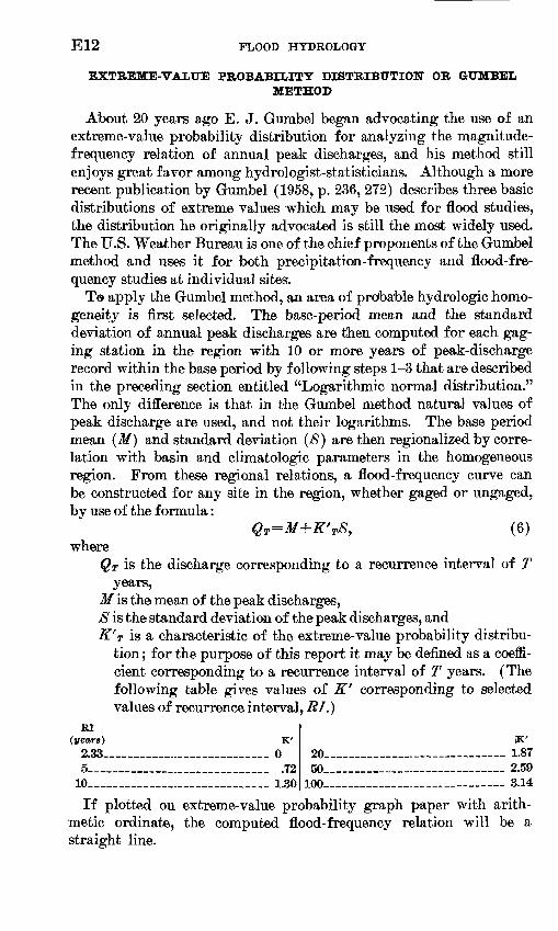
About 20 years ago E. J. Gumbel began advocating the use of an extreme-value probability distribution for analyzing the magnitude- frequency relation of annual peak discharges, and his method still enjoys great favor among hydrologist-statisticians. Although a more recent publication by Gumbel (1958, p. 236, 272) describes three basic distributions of extreme values which may be used for flood studies, the distribution he originally advocated is still the most widely used. The U.S. Weather Bureau is one of the chief proponents of the Gumbel method and uses it for both precipitation-frequency and flood-fre quency studies at individual sites.
To apply the Gumbel method, an area of probable hydrologic homo geneity is first selected. The base-period mean and the standard deviation of annual peak discharges are then computed for each gag ing station in the region with 10 or more years of peak-discharge record within the base period by following steps 1-3 that are described in the preceding section entitled "Logarithmic normal distribution." The only difference is that in the Gumbel method natural values of peak discharge are used, and not their logarithms. The base period mean (M) and standard deviation ($) are then regionalized by corre lation with basin and climatologic parameters in the homogeneous region. From these regional relations, a flood-frequency curve can be constructed for any site in the region, whether gaged or ungaged, by use of the formula:
QT=M+K'T8, (6) where
QT is the discharge corresponding to a recurrence interval of Tyears,
M is the mean of the peak discharges, 8 is the standard deviation of the peak discharges, and K'T is a characteristic of the extreme-value probability distribu
tion ; for the purpose of this report it may be defined as a coeffi cient corresponding to a recurrence interval of T years. (The following table gives values of K' corresponding to selected values of recurrence interval, RI.)
RI (years)
2.33 _______ ..__5_ ________ .
10 ____ __ __.__
K' __ _ _ __ 0
______ .72_ _ _ _ 1.30
20 ___ _ Kt\
100 __ ______ -
IK'
__ ___ _ 1.87_. _ _____ 2.59__ _ _ _ _ 3.14
If plotted on extreme-value probability graph paper with arith metic ordinate, the computed flood-frequency relation will be a straight line.
METHODS USED IN FLOOD-FREQUENCY STUDIES, CALIFORNIA E13
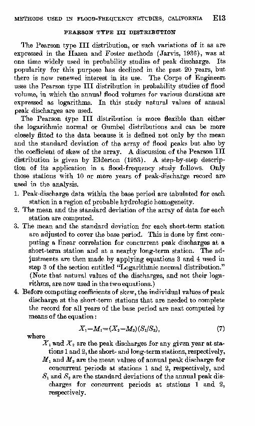
PEARSON TYPE III DISTRIBUTION
The Pearson type III distribution, or such variations of it as are expressed in the Hazen and Foster methods (Jarvis, 1936), was at one time widely used in probability studies of peak discharge. Its popularity for this purpose has declined in the past 20 years, but there is now renewed interest in its use. The Corps of Engineers uses the Pearson type III distribution in probability studies of flood volume, in which the annual flood volumes for various durations are expressed as logarithms. In this study natural values of annual peak discharges are used.
The Pearson type III distribution is more flexible than either the logarithmic normal or Gumbel distributions and can be more closely fitted to the data because it is defined not only by the mean and the standard deviation of the array of flood peaks but also by the coefficient of skew of the array. A discussion of the Pearson III distribution is given by Elderton (1953). A step-by-step descrip tion of its application in a flood-frequency study follows. Only those stations with 10 or more years of peak-discharge record are used in the analysis.1. Peak-discharge data within the base period are tabulated for each
station in a region of probable hydrologic homogeneity.2. The mean and the standard deviation of the array of data for each
station are computed.3. The mean and the standard deviation for each short-term station
are adjusted to cover the base period. This is done by first com puting a linear correlation for concurrent peak discharges at a short-term station and at a nearby long-term station. The ad justments are then made by applying equations 3 and 4 used in step 3 of the section entitled "Logarithmic normal distribution." (Note that natural values of the discharges, and not their loga rithms, are now used in the two equations.)
4. Before computing coefficients of skew, the individual values of peak discharge at the short-term stations that are needed to complete the record for all years of the base period are next computed by means of the equation :
(7) where
JTi and X2 are the peak discharges for any given year at stations 1 and 2, the short- and long-term stations, respectively,
M-L and Mz are the mean values of annual peak discharge forconcurrent periods at stations 1 and 2, respectively, and
$1 and $2 are the standard deviations of the annual peak discharges for concurrent periods at stations 1 and 2,respectively.
E14 FLOOD HYDROLOGY
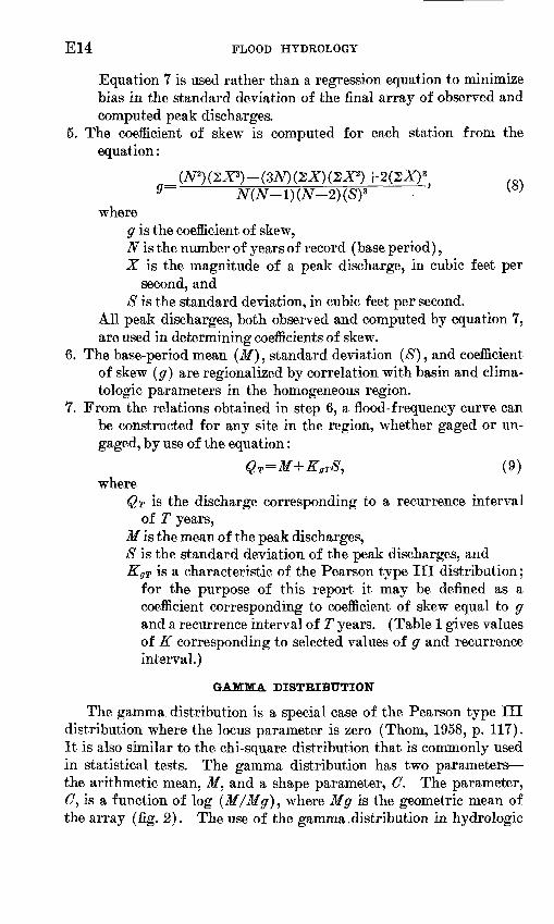
Equation 7 is used rather than a regression equation to minimize bias in the standard deviation of the final array of observed and computed peak discharges.
5. The coefficient of skew is computed for each station from the equation :
9 N(N-l)(N-2)(S)* where
g is the coefficient of skew,N is the number of years of record (base period) ,X is the magnitude of a peak discharge, in cubic feet per
second, andS is the standard deviation, in cubic feet per second.
All peak discharges, both observed and computed by equation 7, are used in determining coefficients of skew.
6. The base-period mean (M) , standard deviation (S) , and coefficient of skew (g) are regionalized by correlation with basin and clima- tologic parameters in the homogeneous region.
7. From the relations obtained in step 6, a flood-frequency curve can be constructed for any site in the region, whether gaged or un- gaged, by use of the equation :
Q T =M+KgTS, (9) where
QT is the discharge corresponding to a recurrence interval of T years,
M is the mean of the peak discharges,S is the standard deviation of the peak discharges, andKg? is a characteristic of the Pearson type III distribution ;
for the purpose of this report it may be defined as a coefficient corresponding to coefficient of skew equal to g and a recurrence interval of T years. (Table 1 gives values of K corresponding to selected values of g and recurrence interval.)
GAMMA DISTRIBUTION
The gamma distribution is a special case of the Pearson type III distribution where the locus parameter is zero (Thorn, 1958, p. 117). It is also similar to the chi-square distribution that is commonly used in statistical tests. The gamma distribution has two parameters the arithmetic mean, M, and a shape parameter, C. The parameter, (7, is a function of log (M/Mg), where Mg is the geometric mean of the array (fig. 2). The use of the gamma .distribution in hydrologic

METHODS USED IN FLOOD-FREQUENCY STUDIES, CALIFORNIA E15
TABLE 1. Pearson type III recurrence curve data, KgT values, in standard deviations from the mean
Skew coefficients (g)
3. 82 i__._ _ <.__ ................3. 0 ..............2.8.............................2.6.... . . -2.4... .... . .... . . ...2.22. 0.... .........................1.9. .... ... ... ........ . ... .1.8 1.7 1.6.............................1.5..... .................1.4... ..... .1.3 . 1.2. 1.11.0.............................0.9 _ __.__..._0.8... . .. ... ....... ..... 0.7 0.6--....--.-...... .... ....0.5 O.4.. ...0.3 0.2 ... . . ... ... ..0.1 0
Recurrence Interval, in years
1.1
-0.65 -.69 -.74 -.80 -.86 -.91 -.93 -.96 -.99
-1.02 -1.04 -1.07 -1.09 -1.11 -1.13 -1.16 -1.18 -1.20 -1.22 -1.24 -1.26 -1.27 -1.29 -1.31 -1.32 -1.33
2
-0.40 -.38 -.37 -.35 -.33 -.31 -.30 -.28 -.27 -.25 -.23 -.22 -.21 -.19 -.18 -.16 -.15 -.13 -.12 -.10 -.08 -.07 -.05 -.03 -.02 0
5
0.45 .48 .51 .55 .58 .61 .62 .64 .66 .68 .70 .72 .73 .74 .75 .76 .77 .78 .79 .80 .81 .82 .82 .83 .84 .84
10
1.18 1.20 1.23 1.25 1.28 1.30 1.31 1.32 1.32 1.33 1.33 1.34 1.35 1.35 1.34 1.34 1.34 1.34 1.33 1.33 1.32 1.32 1.31 1.30 1.29 1.28
20
2.02 2.02 2.01 2.01 2.01 2.00 1.99 1.98 1.97 1.96 1.94 1.93 1.92 1.90 1.89 1.88 1.86 1.84 1.82 1.80 1.77 1.75 1.73 1.70 1.67 1.64
50
23.25 3.13 3.09 3.05 3.00 2.96 2.91 2.88 2.85 2.81 2.77 2.73 2.70 2.67 2.63 2.58 2.54 2.50 2.45 2.41 2.36 2.31 2.26 2.21 2.16 2.11 2.05
100
24.28 4.02 3.95 3.87 3.78 3.70 3.60 3.55 3.50 3.45 3.40 3.34 3.28 3.22 3.15 3.09 3.03 2.96 2.90 2.84 2.77 2.70 2.62 2.55 2.48 2.40 2.33
1 Regional value computed for San Diego area.2 Extrapolated for the purpose of this report.
probability studies has been discussed by Alexander (1962); its ap plication in a flood-frequency study is described below. Only those stations with 10 or more years of peak-discharge record are used in the analysis.
1. Peak-discharge data within the base period are tabulated for each station in a region of probable hydrologic homogeneity.
2. The base-period arithmetic mean (M) for each station in the array is computed, as explained in the earlier discussion of the Gumbel method.
3. The base-period geometric mean (Mg) for each station in the array is computed, as explained in the earlier discussion of the logarith mic normal distribution. (Mg is the antilog of the mean of the logarithms of the peak discharges.)
4. Log (M/Mg) is first computed for each station, and is then used with the curve given in figure 2 to obtain values of the shape parameter, C.
5. The base-period arithmetic mean (M) and the shape parameter (C) are regionalized by correlation with basin and climatologic parameters in the homogeneous region.
6. The regionalized values of M and C are then used with a table of chi-square to obtain the flood-frequency curve for any site in the region whether gaged or ungaged. A table of chi-square can be

E16 FLOOD HYDROLOGY
~l I I FT
0.01 0.1
Log IO (WMg)
FIGURE 2. Relation of C in the gamma distribution to log (M/Mg).
found in any handbook of statistical tables (for example, Arkin and Colton, 1950, p. 121). The number of degrees of freedom (n) to be used in the table is equal to 2(7. Each value of chi- square corresponding to 2(7 degrees of freedom is multiplied by M/2C to give the ordinates of the flood-frequency curve.
7. The use of both logarithms and natural values of discharge in this method is confusing, at first glance. Logarithms are used only in the computation of C; natural values of the peak discharges are used in all other computations.
METHODS USED IN FLOOD-FREQUENCY STUDIES, CALIFORNIA E17
ANALYSIS OF FLOOD FREQUENCY IN THE SAN DIEGOAREA
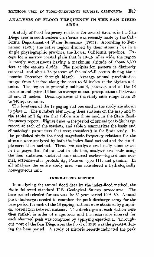
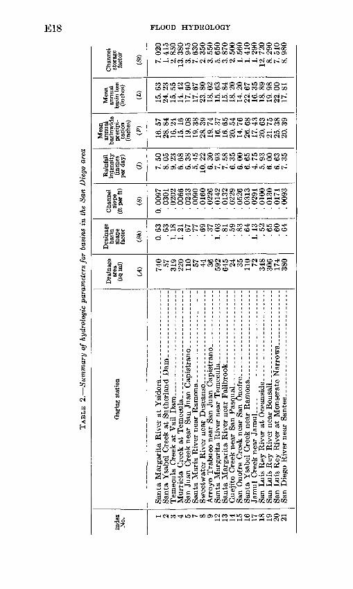
A study of flood-frequency relations for coastal streams in the San Diego area in southwestern California was recently made by the Cali fornia Department of Water Resources (1963). According to Fen- neman (1931) the entire region drained by these streams lies in a single physiographic province, the Lower California province. Ex cept for a narrow coastal plain that is 10-15 miles wide, the region is mostly mountainous having a maximum altitude of about 6,500 feet at the eastern divide. The precipitation pattern is distinctly seasonal, and about 75 percent of the rainfall occurs during the 4 months December through March. Average annual precipitation ranges from 8 inches along the coast to 45 inches at the highest alti tudes. The region is generally subhumid, however, and of the 18 basins investigated, 13 had an average annual precipitation of between 15 and 21 inches. Drainage areas at the study sites range from 24 to 740 square miles.-
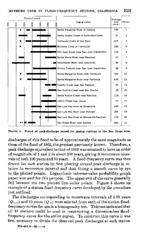
The locations of the 18 gaging stations used in the study are shown in plate 1. The numbers identfying these stations on the map and in the tables and figures that follow are those used in the State flood- frequency report. Figure 3 shows the period of annual peak-discharge record at each of the stations, and table 2 summarizes the basin and climatologic parameters that were considered in the State study. In the published study the flood magnitude-frequency relations for the streams were analyzed by both the index-flood method and the multi ple-correlation method. These two analyses are briefly summarized in the pages that follow, and in addition, analyses are made using the four statistical distributions discussed earlier logarithmic nor mal, extreme-value probability, Pearson type III, and gamma. In all analyses the entire study area was considered a hydrologically homogeneous unit.
INDEX-FLOOD METHOD
In analyzing the annual flood data by the index-flood method, the State followed standard U.S. Geological Survey procedures. The base period selected for use was the 55-year period 1906-60. Annual peak discharges needed to complete the peak-discharge array for the base period for each of the 18 gaging stations were obtained by graphi cal correlation between stations. The discharges at each station were then ranked in order of magnitude, and the recurrence interval for each observed peak was computed by applying equation 1. Through out most of the San Diego area the flood of 1916 was the greatest dur ing the base period. A study of historic records indicated the peak
00
TAB
LE 2.
Sum
mar
y of
hyd
rolo
gic
para
met
ers
for
basi
ns i
n th
e Sa
n D
iego
are
a
Inde
x N
o.
1 2 3 4 5 7 8 9 12 13 14 15 16 17 18 19 20 21
Gag
ing
stat
ion
San
ta M
arga
rita
Riv
er a
t Y
sido
ra _
____
____
__
__
_ _
San
ta Y
sabe
l C
reek
at
Sut
herl
and
Dam
_ __
__
____
____
_T
emec
u la
Cre
ek a
t V
ail
Dam
. _
_ _
_ __
_ __
__
_ __
_M
urri
eta
Cre
ek a
t T
emec
ula.
_ ___
__
__
__
_
San
ta M
aria
Riv
er n
ear
Ram
ona_
___
____
_ __
_ __
_ _
_S
wee
twat
er R
iver
nea
r D
esca
nso_
_
_ __
_ __
____
____
_A
rroy
o T
rabu
co
near
San
Jua
n C
apis
tran
o __
__
____
___
San
ta M
arga
rita
Riv
er n
ear
Fal
lbro
ok__
__
____
_ __
__G
ueji
to C
reek
nea
r S
an P
asqual
. _
_ __
____
____
___
San
Ono
fre
Cre
ek n
ear
San
Ono
fre_
__
_ _
_ __
____
____
_
Jam
ul
Cre
ek n
ear
Jam
ul__
_
____
____
____
____
___
_S
an L
uis
Rey
Riv
er a
t O
cean
side
__
_ -
___
____
___
San
Lui
s R
ey R
iver
at
Mon
sera
te N
arro
ws.
. ___
____
___
_S
an D
iego
Riv
er n
ear
San
tee_
_ _
____
__
_ _
____
____
_
Dra
inag
e ar
ea
(sq
mi)
(A) 74
0 57 319
220
110 57 44 36 592
645 24 35 110 72 348
306
174
380
Dra
inag
e ba
sin
shap
e fa
ctor
(Sft) 0.63 .63
1. 18
1. 2
1.6
7. 7
7.6
9. 3
71.
03 .81
.59
. 83
. 64
1. 13
. 52
.65
.60
.64
Cha
nnel
sl
ope
(ft p
er f
t)
(S)
0. 0
097
.030
1. 0
202
.006
6.0
243
. 009
0.0
16
0. 0
226
. 014
2. 0
132
. 022
9.0
526
. 031
3. 0
291
.01
00
.0130
. 017
1.0
093
Rai
nfal
l in
tens
ity
(inc
hes
per
day)
(/) 7.5
08.
05
9. 2
36.6
86.3
85
.45
10.
226.
30
7.9
37.
58
6. 3
56.
00
6.65
4. 7
55.
93
6. 0
06.
63
7. 3
5
Mea
n an
nual
ba
sin w
ide
prec
ipi
ta
tion
(i
nche
s)
(P)
16.
5728
. 84
16.
2415
. 16
19.
0819
. 38
28.
3919
. 74
16.
3716
.65
20.5
414
. 76
26.6
817
.43
20.
6321
. 75
25.
3820
. 39
Mea
n an
nual
ba
sin
loss
(i
nche
s)
(£)
15.6
324
. 23
15.5
514
.42
17.6
017
.67
23.
8018
.02
15.6
315
. 84
18.
2014
. 20
22.6
716
. 35
18.
8919
. 98
22.
0017
. 81
Cha
nnel
st
orag
e fa
ctor
(SO 7.02
01.
415
2. 8
5013
. 38
03.
945
7.63
02.
350
3. 5
505.6
50
3. 8
702.
500
1. 56
01.
410
1. 29
012
. 72
08.
290
7.51
08.
980
METHODS USED IN FLOOD-FREQUENCY STUDIES, CALIFORNIA E19
Period of record
3000000 Gaging station) f« CM CO *) \C1 <0
«
^
«
t^m
ii
i
^H
^H
_HH .
^^
i
__
^^H
1
t
^H
1
^^H
^^m
mmm
Santa Margarita River at Ysidora
Santa Ysabel Creek at Sutherland Dam
i Temecula Creek at Vail Dam
Murrieta Creek at Temecula
San Juan Creek near San Juan Capistrano
Santa Maria River near Ramona
Sweetwater River near Descanso
Arroyo Trabuco near San Juan Capistrano
Santa Margarita River near Temecula
Santa Margarita River near Fallbrook
Guejito Creek near San Pasqual
San Onofre Creek near San Onofre
Santa Ysabel Creek near Ramona
Jamul Creek near Jamul
San Luis Rey River at Oceanside
San Luis Rey River near Bonsall
San Luis Rey River at Monserate Narrows
San Diego River near Santee
Drainage area
(sq mi)
740
57
319
220
110
57
44
36
592
645
24
35
110
72
348
306
174
380
Station
1
2
3
4
5
7
8
9
12
13
14
15
16
17
18
19
20
21
FIGURE 3. Period of peak-discharge record for gaging stations In the San Diego area.
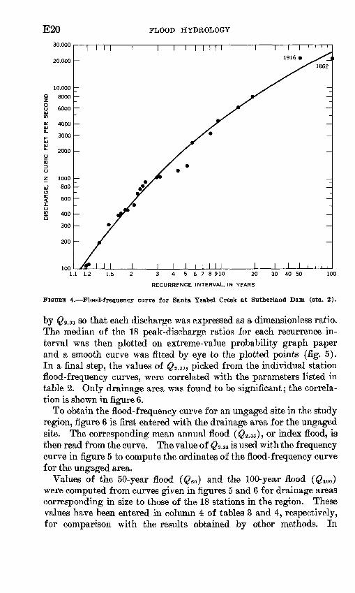
discharges of this flood to be of approximately the same magnitude as those of the flood of 1862, the greatest previously known. Therefore, a peak discharge equivalent to that of 1916 was assumed to have an order of magnitude of 1 and 2 in about 100 years, giving it recurrence inter vals of both 100 years and 50 years. A flood-frequency curve was then drawn for each station by first plotting annual peak discharge in re lation to recurrence interval and then fitting a smooth curve by eye to the plotted points. Logarithmic extreme-value probability graph paper was used for this purpose. The upper end of the curve generally fell between the two plotted first-order points. Figure 4 shows an example of a station flood-frequency curve developed by the procedure just outlined.
The discharges corresponding to recurrence intervals of 2.33 years ($2.33) and 10 years (Qw ) were selected from each of the station flood- frequency curves for use in a homogeneity test. This test indicated that all 18 stations could be used in constructing a dimensionless flood- frequency curve for the entire region. To construct this curve it was first necessary to divide the observed peak discharges at each station
TtfO-401i
E2030,000
20,000
10,000
Q 8000
8 6000LJwg 4000o.
3000
FLOOD HYDROLOGY
2000
1000800
600
400
300
100
i i n
i i i1.1 1.2 3 45678910 20
RECURRENCE INTERVAL, IN YEARS
30 40 50
FIGUEB 4. Flood-frequency curve for Santa Ysabel Creek at Sutherland Dam (sta. 2).
by $2.33 s° that each discharge was expressed as a dimensionless ratio. The median of the 18 peak-discharge ratios for each recurrence in terval was then plotted on extreme-value probability graph paper and a smooth curve was fitted by eye to the plotted points (fig. 5). In a final step, the values of $2.33, picked from the individual station flood-frequency curves, were correlated with the parameters listed in table 2. Only drainage area was found to be significant; the correla tion is shown in figure 6.
To obtain the flood-frequency curve for an ungaged site in the study region, figure 6 is first entered with the drainage area for the ungaged site. The corresponding mean annual flood ($2.33)? or index flood, is then read from the curve. The value of $2.33 is used with the frequency curve in figure 5 to compute the ordinates of the flood-frequency curve for the ungaged area.
Values of the 50-year flood (Q50 ) and the 100-year flood ($100) were computed from curves given in figures 5 and 6 for drainage areas corresponding in size to those of the 18 stations in the region. These values have been entered in column 4 of tables 3 and 4, respectively, for comparison with the results obtained by other methods. In

METHODS USED IN FLOOD-FREQUENCY STUDIES, CALIFORNIA E21
column 3 of these tables are listed the values ofQ50 and ^100? picked from the individual station curves, such as the curve shown in figure 4.
MULTIPLE CORRELATION
The same 18 stations in the San Diego area were also analyzed by the California Department of Water Resources (1963), using the multiple-correlation method. The 55-year base period, 1906-60, was again used, and the entire region was considered hydrologically homogeneous. From the individual station flood-frequency curves (such as the curve given in fig. 4) constructed for the index-flood method of analysis, discharges corresponding to various recurrence intervals were read. For this study we are interested only in the discharges corresponding to recurrence intervals of 50 years (Q50 ) and 100 years (Qi00 ). All values of Q 50 were correlated with the basin and climatologic parameters shown in table 2; similar correlations were made for values of $100- It was found that the only statistically
Q
O 10
1.0
0.11.2 1.3 1.5 3 4 5678910 20
RECURRENCE INTERVAL, IN YEARS
30 40 50 100
FIGURE 5. Dimensionless regional flood-frequency curve for the San Diego area (index- flood method).

E22 FLOOD HYDROLOGY
O 2000
OCD 800
a 400
10 20 50 100 200 500 1000
DRAINAGE AREA, IN SQUARE MILES
FIGURE 6. Relation of mean annual flood to drainage area in the San Diego area (index- flood method).
significant parameters were drainage area (A) and a drainage basin shape factor (Sh). This shape factor is defined as the ratio of the diameter of a circle of area equal to basin area to the length of the basin measured parallel to the principal channel. The following regression equations were obtained:
^5 o = 1016^L 0 - 59^-0 - 44 (10)
and^100 =1288^0 - 60^-0 - 57 . (11)
For each equation the coefficient of correlation was 0.954.For later comparison in the section entitled, "Discussion of results
of the analysis," the values of Q50 and $100, computed for the 18 sta tions by application of these equations, have been entered in column 6 of tables 3 and 4, respectively.
LOGARITHMIC NORMAL DISTRIBUTION
A regional flood-frequency curve for the San Diego region was com puted by fitting a logarithmic normal distribution to the original base data. This was done to compare the results with those obtained by other methods. The first step in the computation was to convert the natural values of peak discharge to logarithms. None of the 18 gag ing stations had peak-discharge records that were complete for the

TAB
LE 3
. Q
so f
or s
trea
ms
in t
he S
an D
iego
are
a as
det
erm
ined
fro
m g
raph
ical
ly d
eriv
ed f
lood
-fre
quen
cy c
urve
s an
d by
var
ious
met
hods
of
regi
onal
floo
d-fr
eque
ncy
anal
ysis
Inde
x N
o. 1 1 2 3 4 5 7 8 9 12
13
14
15
16
17
18
19
20
21
Stat
ion
2
Qso
from
gr
aph
ic
ally
- de
rive
d st
atio
n cu
rves
(c
fs) 3
54,0
00
17,0
00
24,0
00
24,5
00
26,0
00
9,30
0 10
,500
13
,400
36
,500
50
,000
5,
500
9,90
0 23
,600
13
,000
32
,000
36
,000
27
,000
54
,000
Inde
x-flo
od
met
hod
Qso
(cfs
)
4
50,8
00
13,3
00
32,9
00
27,3
00
18,9
00
13,3
00
11,6
00
10,5
00
45,4
00
47,7
00
8,52
0 10
,400
18
,900
15
,200
34
,400
32
,100
24
,000
36
,400
Perc
ent
diff
er
ence
fr
om
col.
3
5 -6
-22
+
37
+11
-2
7
+43
+
10
-22
+
24
-5
+55
+
5
-20
+17
+
8
-11
-1
1
-33
Mul
tiple
co
rrel
atio
n
Qso
(cfs
)
6
60,0
00
13,5
00
28,0
00
22,0
00
19,0
00
12,5
00
11,0
00
13,0
00
42,5
00
50,0
00
8,40
0 8,
900
19,5
00
12,0
00
42,0
00
36,0
00
27,0
00
40,0
00
Perc
ent
diff
er
ence
fr
om
col.
3
7 +11
-21
+17
-10
-27
+34
±1
+16 0
+53
-10
-17 -8
+31 0 0
-26
Log
arith
mic
no
rmal
di
stri
butio
n
Qso
(cfs
)
8
99,8
00
15,5
00
53,2
00
42,3
00
25,4
00
15,5
00
13,0
00
11,4
00
83,6
00
89,0
00
8,59
0 11
,100
25
,400
18
,600
56
,200
52
,400
35
,400
60
,400
Perc
ent
diff
er
ence
fr
om
col.
3
9 +85
-9
+
122
+73
-2
+
67
+24
-1
5
+12
9 +
78
+56
+12
+
8
+43
+
76
+46
+
31
+12
Ext
rem
e-va
lue
prob
abili
ty
dist
ribu
tion
Qso
(cfs
)
10
28,7
00
8,53
0 19
,300
16
,200
11
,600
8,
530
7,53
0 6,
830
25,7
00
26,9
00
5,67
0 6,
730
11,6
00
9,51
0 19
,900
18
,800
14
,500
21
,000
Perc
ent
diff
er
ence
fr
om
col.
3
11 -47
-5
0
-20
-34
-55
-8
-28
-49
-30
-46
+3
-32
-5
1
-27
-38
-48
-46
-61
Pear
son
type
II
I di
stri
butio
n
Qso
(cfs
)
12
34,6
00
10,4
00
23,4
00
19, 7
00
14,1
00
10,4
00
9,16
0 8,
300
31,1
00
32,6
00
6,90
0 8,
180
14,1
00
11,6
00
24,1
00
22,8
00
17,6
00
25,4
00
Perc
ent
diff
er
ence
fr
om
col.
3
13 -36
-39
-2
-20
-46
+12
-1
3
-38
-15
-35
+25
-1
7
-40
-11
-25
-37
-35
-53
Gam
ma
dist
ribu
tion
Qso
(cfs
)
14
28,9
00
7,59
0 18
,600
15
,200
10
,600
7,
590
6,60
0 5,
960
25,7
00
26,9
00
4,79
0 5,
840
10,6
00
8,58
0 19
,400
18
,200
13
,600
20
,400
Perc
ent
diff
er
ence
fr
om
col.
3
15 -46
-55
-22
-38
-59
-18
-37
-56
-30
-46
-13
-41
-55
-34
-39
-49
-50
-62
O O to GO

fe)
TABL
E 4
. Qi
oo f
or s
trea
ms
in t
he S
an D
iego
are
a as
det
erm
ined
fro
m g
raph
ical
ly
deri
ved
flood
-fre
quen
cy
curv
es
and
by v
ario
usm
etho
ds o
f re
gion
al f
lood
-fre
quen
cy a
naly
sis
Inde
xN
o. 1
1 2 3 4 5 7 8 9 12
13
14
15
16
17
18
19
20
21
Sta
tion
2
Tem
ecul
a C
reek
at
Vai
l D
am..
__
__
__
__
_ _
__
Qioo
fro
m
gran
h-
deri
ved
stat
ion
curv
es
(cfs
) 3
72,0
00
26,0
00
34,0
00
27,5
00
36,5
00
12,8
00
15,5
00
18,5
00
49,0
00
67,0
00
7,20
0 13
,300
30
,500
17
,000
52
,000
50
,000
39
,000
75
,000
Inde
x-flo
od
met
hod
Qioo
(o
b) 4
70,5
00
18,5
00
45,7
00
37,8
00
26,2
00
18,5
00
16,2
00
14,6
00
63,0
00
66,2
00
11,8
00
14,4
00
26,2
00
21,1
00
47,7
00
44,5
00
33,3
00
50,4
00
Per
cent
di
ffer
en
ce
from
co
l. 3
5 -2
-29
+34
+
37
-28
+
45
+5
-2
1 +
29
-1
+64
+
8
-14
+
24
-8
-11
-15
-33
Mul
tiple
co
rrel
atio
n
Qioo
(c
fs)
6
86,0
00
18,5
00
37,0
00
28,5
00
26,5
00
16,5
00
15,5
00
19,0
00
57,0
00
68,5
00
11,5
00
12,0
00
27,0
00
15,5
00
60,0
00
50,0
00
37,0
00
56,0
00
Per
cent
di
ffer
en
ce
from
co
l. 3
7 +19
-2
9
+9
+4
-2
7
+29
0 +
3
+16
+
2
+60
-1
0
-11
-9
+15
0 -5
-2
5
Log
arith
mic
no
rmal
di
stri
buti
on
Qioo
(c
fs)
8
190,
000
27,0
00"
98,2
00
77,4
00
45,4
00
27,0
00
22,4
00
19,6
00
158,
000
168,
000
14,6
00
19,1
00
45,4
00
32,7
00
104,
000
96,6
00
64,2
00
112,
000
Per
cent
di
ffer
en
ce
from
co
l. 3
9
+16
4 +
4
+18
9 +
181
+24
+
111
+45
+
6
+22
2 +
151
+10
3 +
44
+49
+
92
+10
0 +
93
+65
+
49
Ext
rem
e-va
lue
prob
abil
ity
dist
ribu
tion
Qioo
(c
fs)
10
33,6
00
10,0
00
22,6
00
19,1
00
13,7
00
10,0
00
8,88
0 8,
050
30,1
00
31,6
00
6,69
0 7,
930
13,7
00
11,2
00
23,4
00
22,1
00
17,0
00
24,7
00
Per
cent
di
ffer
en
ce
from
co
l. 3
11 -53
-62
-34
-31
-62
-22
-4
3
-56
-39
-5
3
-7
-40
-5
5
-34
-55
-5
6
-56
-6
7
Pear
son
type
II
I di
stri
buti
on
Qioo
(c
fs)
12
44,2
00
13,2
00
29,7
00
25,1
00
18,0
00
13,2
00
11,7
00
10,6
00
39,5
00
41,4
00
8,82
0 10
,500
18
,000
14
,800
30
,700
29
,000
22
,400
32
,400
Per
cent
di
ffer
en
ce
from
co
l. 3
13 -39
-4
9
-13
-9
5
1
+3
-25
-4
3
-19
-3
8
+22
-2
1 -4
1 -1
3
-41
-42
-43
-57
Gam
ma
dist
ribu
tion
Qioo
(c
fs)
14
35,3
00
9,26
0 22
,700
18
,600
12
,900
9,
260
8,05
0 7,
270
31,3
00
32,8
00
5,84
0 7,
120
12,9
00
10,5
00
23.7
00
22,2
00
16,5
00
24,9
00
Per
cent
di
ffer
en
ce
from
co
l. 3
15 -51
-64
-33
-3
2
-65
-2
8
-48
-6
1 -3
6
-51
-19
-4
6
58
-38
-54
-5
6
-58
-67
METHODS USED IN FLOOD-FREQUENCY STUDIES, CALIFORNIA E25
entire 55-year base period, 1906-60. The next step was to select a few stations that were strategically located for use as base stations, and then to estimate the logarithms of the annual peak discharges needed to complete the 55-year array for these stations. Three of the stations having comparatively long records, stations 2, 3, and 8, were chosen as base stations, and the required individual logarithms of peak discharge were computed by use of equation 7. (Note that logarithms are used at this time in equation 7 and not natural values.) The use of equation 7, instead of a regression equation, results in a less biased estimate of the standard deviation of the 55-year array of annual peak discharges, not all of which are observed.
The mean and the standard deviation for the 55-year array at each of the three base stations were then computed. After this was done, the mean and the standard deviation of each of the remaining 15 short-term records were first computed and then adjusted to the 55- year base period by correlation with a base station. Equations 3 and 4 were then applied to the results. At this stage of the computa tions the base-period mean (M) and standard deviation ($) were available for all 18 stations. The values of M and $, still in loga rithmic units, were next regionalized by correlation with the basin and climatologic parameters in table 2. Of these parameters, only drainage area was statistically significant. The two graphs in figure 7 show the relations between (1) drainage area and M, the mean of the logarithms of peak discharge; and (2) drainage area and $, the standard deviation of the logarithms of discharge. By use of these two graphs and equation 5, a flood-frequency curve can be computed for any site in the region. Specific equations for computing Q50 and $10o, in logarithmic units, are:
<? 60 =M+2.05£ (12) and
<? 100 =Jl/+2.33£. (13)
Values of Q50 and $100, in logarithms, were computed from curves given in figure 7 and by application of equations 12 and 13, respec tively, for drainage areas corresponding in size to those of the 18 gaging stations. The antilogarithms of Q50 and Quo have been en tered in column 8 of tables 3 and 4, respectively, for later comparison.
EXTREME-VALUE PROBABILITY DISTRIBUTION OB GUMBELMETHOD
A regional flood-frequency study of the San Diego region was also made by fitting an extreme-value probability distribution to the original base data. In this analysis natural values of the discharges were used, and not their logarithms. Stations 2, 3, and 8 were again

E26 FLOOD HYDROLOGY
50 100 200
DRAINAGE AREA, IN SQUARE MILES
500 1000
FIGURE 7. Relation of mean and standard deviation of logarithms of annual peak discharges to drainage area in the San Diego area.
made the base stations for the study and their records were completed for the 55-year base period by use of equation 7. The mean and the standard deviations for the 3 base stations and the 15 short-term sta tions were then computed. These statistics for the short-term records were adjusted to the 55-year base period by correlations with a base station. Equations 3 and 4 were then applied to the results. (Note that natural values are used in this method in equations 3 and 4.) The resulting base-period values of the mean (M) and standard devi ation ($) were regionalized by correlation with the basin and clima- tologic parameters listed in table 2. Again, drainage area was the only statistically significant parameter. The two graphs in figure 8 show the relation between (1) drainage area and J/, and (2) drainage area and S. By use of these two graphs and equation 6, a flood-f requen-

METHODS USED IN FLOOD-FREQUENCY STUDIES, CALIFORNIA E27
cy curve can be computed for any site in the region. Specific equations for computing Q5Q and Qwo are:
and
10,000
8000
6000
5000
4000
3000
2000
1000
800
600
20,000
10,000
8000
6000
5000
4000
3000
2000
21
20
1000
,16
8«
20 50 100 200 500 1000
DRAINAGE AREA, IN SQUARE MILES
FIGURE 8. Relation of mean and standard deviation of annual peak discharges to drainage area in the San Diego area.
770-401 O - 65 - 5

E28 FLOOD HYDROLOGY
Values of Q50 and QW o were computed from curves given in figure 8 and by application of equations 14 and 15, respectively, for drainage areas corresponding in size to those of the 18 gaging stations. These values are listed in column 10 of tables 3 and 4, respectively, for later comparison.
PEABSON TYPE III DISTBIBUTION
A fifth flood-frequency analysis was made for the San Diego area streams by fitting a Pearson type III distribution to the peak- discharge data. The computation and regionalization of the base- period mean (M) and standard deviation ($) for this study are identical with those for the extreme-value probability analysis. Con sequently, the graphs in figure 8 were applicable to this analysis. The next step was to determine the coefficient of skew for each station. This was done by first using equation 7 to compute the annual peak discharges needed to complete the 55-year array at each short- term station and then using equation 8 to compute the coefficient of skew (g) for each station. The individual values of g ranged from 2.39 to 5.35 but showed no correlation with basin or climatologic parameters. Consequently, the average value of g, 3.82, was assumed to be its regional value. A flood-frequency curve can be computed for any site in the region, gaged or ungaged, by first entering figure 8 with drainage area to obtain M and /S and then using equation 9 and table 1 with the regional skew of 3.82.
Values of Q50 and Q100 were computed by use of the relations and table just mentioned for drainage areas corresponding in size to those of the 18 gaging stations. These values have been entered in column 12 of tables 3 and 4, respectively, for later comparison with the results obtained by the other methods of analysis.
GAMMA DISTBIBUTION
The gamma distribution was also used to analyze the flood magni tude-frequency relation for streams in the San Diego area. A pre requisite to the use of this method was a determination of the base-period arithmetic mean (M) and geometric mean (Mg) for each of the 18 stations. Values of M were available from the previous use of the Gumbel-method analysis, and the logarithms of Mg were available from the previous use of the logarithmic normal distribution. The logarithms of Mg were then converted to natural values. The logarithm of the ratio M/Mg was next computed for each station, and the curve given in figure 2 was then used to obtain corresponding values of C. The next step was to regionalize the values of M and C. This had been done for M in the Gumbel method of analysis and the results are found in figure 8. The individual values of C ranged from
METHODS USED IN FLOOD-FREQUENCY STUDIES, CALIFORNIA E29
0.31 to 0.89, but showed no correlation with basin or climatologic parameters. Consequently, the average value of £7, 0.43, was assumed to be its regional value. The regional values of M and O can be used with a table of chi-square to compute a flood-frequency curve for any site in the region, whether gaged or ungaged.
Values of Q$Q and QWQ were computed by use of curves given in figure 8, a regional value of O of 0.42, and a chi-square table, for drainage areas corresponding in size to those of the 18 gaging stations. These values are listed in column 14 of tables 3 and 4, respectively, for later comparison with the results obtained by the other five methods of analysis.
ANALYSIS OF FLOOD FREQUENCY IN NORTH COASTALCALIFORNIA
A study of flood-frequency relations for coastal streams in northern California was recently made by the U.S. Geological Survey (Eantz, 1964, p. 60-73). According to Fenneman (1931), the region drained by these streams lies in two physiographic sections the northern California Coast Ranges and the Klamath Mountains. Except for a narrow coastal plain, the region is very mountainous with many peaks above an altitude of 6,000 feet. The precipitation is distinctly seasonal and about 75 percent of it occurs during the 5 months, Novem ber through March. Snow falls in moderate amounts at altitudes above 2,000 feet, but only at altitudes above 4,000 feet does snow remain on the ground for appreciably long periods. Average annual precipi tation increases from east to west, ranging from a low of 10 inches in the Shasta Eiver valley to a high of 120 inches in the upper Smith River basin. The region as a whole is very humid; and of the 27 basins investigated, only 5 had an average annual precipitation of less than 50 inches. Drainage areas at the study sites ranged from 6 to 12,000 square miles.
The locations of the 27 gaging stations used in the study are shown in plate 2. The numbers identifying these stations on the map and in the tables and figures that follow are those listed in the Geological Survey study. Figure 9 shows the period of annual peak-discharge record at each of the stations, and table 5 lists the two hydrologic parameters drainage area and mean annual precipitation that were found to have a significant effect on the flood magnitude-frequency relation. In the Geological Survey study this relation was analyzed by the index-flood method. That analysis is summarized in the pages that follow, and in addition, analyses were made by five other meth ods multiple correlation, logarithmic normal distribution, extreme- value probability distribution, Pearson type III distribution, and the

Pe
rio
d o
f re
cord
-> o
o
o
o
o
Gagin
g s
tation
-H CM
co
^-
m
io
n
CTI
o>
CTI
CTI
ff>
I
1_ m
^ B
IMH
H
IM
IHB
H
__
Co
ast
Ra
ng
es
East
Fork
Russ
ian R
iver
near
Calp
ella
Mid
dle
Fork
Eel
Riv
er
belo
w B
lack
Bu
tte
Riv
er
near
Cove
lo
Eel
Riv
er
belo
w D
os R
ios
No
rth
For
k E
el R
iver
near
Min
a
South
For
k E
el R
iver
near
Bra
nsc
om
b
South
For
k E
el R
iver
near
Miranda
Eel
Riv
er
at
Sco
tia
Van
Duz
en R
ive
r near
Din
smo
res
Van
Duz
en R
iver
near
Brid
ge
ville
Yager
Cre
ek
near
Ca
rlo
tta
Jaco
by
Cre
ek
near
Fre
shw
ate
r
Ma
d R
iver
near
Fo
rest
Gle
n
Mad
Riv
er
near
Arc
ata
Re
dw
oo
d C
ree
k near
Blu
e L
ake
Re
dw
oo
d C
ree
k at
Orick
Dra
ina
ge
are
a
(sq
mi)
93
367
1481 251 43
.9
537
3113
80.2
214
127 6.
07
144
485 67
.5
278
Sta
tion
4615
47
30
4740
4745
4755
4765
4770
4775
4785
4790
4800
4805
4810
4815
4825
CO o

METHODS USED IN FLOOD-FREQUENCY STUDIES, CALIFORNIA E31
DO (0C
(0
Q
oo
iod of rec
q)
O.
c o
(0
co
ra g
o !n^
c o<n
Gaging st:
0961
0961
0*6 1
OE6I
0261
DTfiT
if) If) if) u tv o> CM ui-H i-l CM C
If) IT) If) u
tv CM IO I If) Id <* C10 10 rv r
inC
5
|
^ 4) (5£ _ C jara S o «
I 1 r E :^ *" o o
>- U- C/5 *" k. +J -5. TO W H
<" k.SJ >. > 1 .1 = c^ ^ 0to t; p (5 t> i£ 0 (5C/5 C/5 C/5 h
1
1
.
nooif)oof)oif) niorvOoooocMCMMCMCMCMCMrorororoDiDiDLniDiniDiDin
orvooooioof)^Nl I-H CO f^ O^ ^ O O^ I""1 vo^rooooOrtCMio
- CM CM
^
b.
Ck. 0) 0) O> in (u
£ S E ^ « gO c o «j £ O
» £ p £ « 1 ?-WC(OC C Q
2S?E>Sio ff'«w ^oa^'-o^.Stt)
1 ° ? > ^ « " «J » Q) ^i tl fl)-^ ^
- 8 8 c c 8 £ | g\)cc^-cc>-Ec
k.k.<U|-k.5W^
^55g^^|^5 eircc^oa:.cO£
^cc'x'ScE^--z 'z 'c w o 'ki J2 o c-Hl-IWI-yWW
1 1 1 1I
1
1
|M
j"
t4^
t
iic\t4
1<(
(*
I (1
5i i i i
i
« c*
1
iiiji ic
<bc
1 i«p
0E BCte

E32 FLOOD HYDROLOGY
gamma distribution. In differentiating regional characteristics of Qz.zz in the index-flood method and in all subsequent analyses of the data for north coastal California, each of the two physiographic sections the Coast Ranges and the Klamath Mountains was con sidered separately as a hydrologic entity.
TABLE 5. Summary of pertinent hydrologic parameters for basins in northcoastal California
[Asterisk indicates long-term station]
Index No.
Gaging station Drainage area (sq mi)
Mean annual
basin wide precip itation (inches)
Coast Ranges
*4615 East Fork Russian River near Calpella__________ 93. 04730 Middle Fork Eel River below Black Butte River,
near Covelo_______.______________________ 3674740 Eel River below Dos Rios____________________ 1,4814745 North Fork Eel River near Mina_____________ 251
*4755 South Fork Eel River near Branscomb_________ 43. 9*4765 South Fork Eel River near Miranda___________ 537*4770 Eel River at Scotia_____________.______ 3,1134775 Van Duzen River near Dinsmores.______________ 80. 2
*4785 Van Duzen River near Bridgeville_____________ 2144790 Yager Creek near Carlotta__________--._-____ 1274800 Jacoby Creek near Freshwater._________________ 6. 074805 Mad River near Forest Glen_________________ 1444810 Mad River near Arcata_______________--------_ 4854815 Redwood Creek near Blue Lake_______________ 67. 54825 Redwood Creek at Orick_______________ 278
Elamath Mountains
*5175 Shasta River near Yreka_________________ » 657*5195 Scott River near Fort Jones________________ 662*5225 Salmon River at Somesbar______________-_---_- 746*5255 Trinity River at Lewiston________________ 726
5260 Trinity River near Douglas City_____________ 1,017*5270 Trinity River near Burnt Ranch._______________ 1, 4385285 Hayfork Creek near Hyampom_________________ 3795290 South Fork Trinity River near Salyer_______ _ 899
*5300 Trinity River near Hoopa__________________ 2,846*5305 Klamath River near Klamath._______________ 12, 100
5320 South Fork Smith River near Crescent City__ __ 295*5325 Smith River near Crescent City_______________ 613
40
6053587970597472605460648080
19335759565743505542116111
1 Actual drainage area above gage is 796 sq mi, but 139 sq mi above Dwinnell Reservoir is noncontributing.

METHODS USED IN FLOOD-FREQUENCY STUDIES, CALIFORNIA E33
INDEX-FLOOD METHOD
In analyzing the annual flood data by the index-flood method, Rantz (1964) used a 28-year base period, 1932-59. Of the 27 gaging stations studied, only 13 had records with 10 or more years within the base period. Annual peak discharges needed to complete the discharge array for the base period for these 13 stations were obtained by graphi cal correlation. The discharges at each of the stations were then ranked in order of magnitude, and the recurrence interval for each observed peak was computed by applying equation 1. A flood-frequency curve was next drawn on extreme-value probability graph paper for each of the 13 stations by first plotting annual peak discharge against re currence interval and then fitting a smooth curve by eye to the plotted points.
It was possible to extrapolate the flood-frequency curves beyond the base period with considerable confidence because of the availability of historical records, both qualitative and quantitative, of major floods that occurred in years prior to 1932. For Klamath Eiver at Klamath (sta. 5305), the magnitudes of all major flood peaks in the past 106 years are known and were used in the construction of the flood- frequency curve (fig. 10). For other stations, where it was known only that the flood peaks of 1956 were roughly equivalent to those of 1862 and greater than any other since at least 1854, the magnitude of
500,000
450,000
400,000
y 250,000
? 200,000
EXPLANATION
Peak discharges that oc
curred within the base period, 1932-59
OPeak discharges that oc
curred prior to the base period
3 4 5 6 8 10 20
RECURRENCE INTERVAL, IN YEARS
FIGURE 10. Flood-frequency curve for Klamath River at Klamath (sta. 5305).
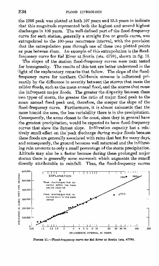
E34 FLOOD HYDROLOGY
the 1956 peak was plotted at both 107 years and 53.5 years to indicate that this magnitude represented both the highest and second highest discharges in 106 years. The well-defined part of the flood-frequency curve for each station, generally a straight line or gentle curve, was extrapolated to the 100-year recurrence interval, with the provision that the extrapolation pass through one of these two plotted points or pass between them. An example of this extrapolation is the flood- frequency curve for Eel Eiver at Scotia (sta. 4770), shown in fig. 11.
The slopes of the station flood-frequency curves were next tested for homogeneity. The results of this test are better understood in the
'light of the explanatory remarks that follow. The slope of the flood- frequency curve for northern California streams is influenced pri marily by the difference in severity between the storms that cause the milder floods, such as the mean annual, flood, and the storms that cause the infrequent major floods. The greater the disparity between these two types of storm, the greater the ratio of major flood peak to the mean annual flood peak and, therefore, the steeper the slope of the flood-frequency curve. Furthermore, it is almost axiomatic that the more humid the area, the less variability there is in the precipitation. Consequently, the areas closest to the coast, since they in general have the greatest precipitation, would be expected to have flood-frequency curves that show the flattest slope. Infiltration capacity has a rela tively small effect on the peak discharge during major floods because these floods are generally associated with rains that last for many days, and consequently, the ground becomes well saturated and the infiltrat ing rain amounts to only a small percentage of the storm precipitation. Altitude may also be a factor because during these prolonged major storms there is generally some snowmelt which augments the runoff directly attributable to rainfall. Thus, the flood-frequency curves
600,000
O 300,000
5 200,000
I Inil i iEXPLANATION
I I I I
Peak discharges that oc curred within the base period, 1932-59
OPeak discharges that oc
curred prior to the base period
3 4 5 6 8 10 20
RECURRENCE INTERVAL, IN YEARS
FIGURE 11. Flood-frequency curve for Bel River at Scotia (sta. 4770).

METHODS USED IN FLOOD-FREQUENCY STUDIES, CALIFORNIA. E35
for the basins of higher altitude in northwestern California tend to have steeper slopes.
The statistical tests for homogeneity of slope of the flood-frequency curves bore out these premises. These tests resulted in the establish ment of the three areas of homogeneity shown in plate 2. The dimen sions flood-frequency curves for the three subregions are plotted in figure 12. Subregion 1 has the flattest station flood-frequency curves; lying closest to the ocean, it is the most humid area and has the lowest altitude. Its dimensionless flood-frequency curve is based on the eight gaging stations in subregion 1 that had been in operation for at least 10 years. The slope of the dimensionless flood-frequency curve for subregion 2 is steeper than that of the flood-frequency curve for sub- region 1 owing «& the generally more variable storm precipitation and higher altitudes found in subregion 2. Only three stations have 10 or more years of record in subregion 2, and consequently the flood- frequency curve representative of this subregion lacks the high degree of confirmation obtainable from a large number of gaging stations. The fact that the dimensionless flood-frequency curve for subregion 3 has the steepest slope of the three regional curves reflects that sub- region 3 is the least humid of the three subregions. Only two stations in the subregion have the requisite 10 or more years of record.
The magnitude of the mean annual flood ($2.33) was next investi gated. For the 13 stations with 10 or more years of peak-discharge record, $2.33 was picked from the individual station flood-frequency
I I I TIT
6 7 8 9 10 20
RECURRENCE INTERVAL, IN YEARS
FIGURE 12. Dimensionless regional flood-frequency curves for north coastal California(index-flood method).
E36 FLOOD HYDROLOGY
curves that had been previously plotted. For the 14 stations with less than 10 years of record, correlation procedures were used to determine $2.33- Concurrent peak discharges for each of these short-term sta tions and for a nearby longer term station were correlated graphi cally. $2.33 for the short-term station was then determined from the regression line, it being the discharge corresponding to $2.33 for the longer-term station. The values of Q 2.33 for both long-term and short- term stations were then analyzed.
The magnitude of the mean annual flood in basins in northwestern California is related primarily to the size of drainage area and to the magnitude of the mean annual storm. Mean annual precipitation is an excellent index of the relative magnitude of the mean annual storm because the bulk of the annual precipitation in the region occurs during several general storms each year, and all stations experience the same number of general storms in any given year. Subsurface storage also exerts a significant influence on the magnitude of the mean annual flood. Surface storage, on the other hand, is a negligible factor in this study because there are no sizable lakes or reservoirs that are uncon trolled, and streams that are seriously affected by artificially regulated storage were excluded from the analysis. Because subsurface storage is related to the infiltration capacity, or the permeability of the soil and mantle rock, and because much greater permeability is associated with the Klamath Mountains than with the Coast Ranges, it is logical to expect the mean annual flood to differ in these two physiographic sections, when all other factors are equal.
In figure 13 the mean annual floods for basins in the Coast Eanges have been plotted in relation to the drainage area. Each point is la beled with (1) the number of the gaging station for identification, and (2) the mean annual precipitation for the basin upstream from the station. (Drainage area and mean annual basin wide precipitation are given in table 5.) Precipitation in the Coast Ranges basins ranges from 40 to 80 inches, and within this range no significant correlation is apparent between mean annual flood ancTmean annual precipitation. A straight line averaging the plotted points has the equation:
Mean annual flood (£2 . 33 ) = 130J.0- 91, (16)
where A is the drainage area in square miles.The wide range in mean annual precipitation in the Klamath Moun
tains, 19-116 inches, has a very pronounced effect on the magnitude of the mean annual flood. The relation of $2.33 to drainage area and mean annual precipitation in this physiographic section can be ex pressed by a means of a family of curves, each of which has an equa tion similar to equation 16. The equation for this family of curves is

METHODS USED IN FLOOD-FREQUENCY STUDIES, CALIFORNIA E37
200,000
100,000
80,00070,00060,00050,000
40,000
30,000
20,000
10,000
8000700060005000
4000
3000
2000
1000
800700600500
T I I I IT
EXPLANATION
80
Upper number is gaging station. Lower number is mean annual basin- wide precipitation, in inches.
Equation of curve: Q 2.33 =130A°»
10 10 Is* oo o o oooooo oo «* in 10 rv oo o
DRAINAGE AREA, IN SQUARE MILES
FIGURE 13. Relation of mean annual flood to drainage area in the Coast Ranges (index- flood method).
where C is a variable that is related to mean annual precipitation. The relation of C to mean annual basinwide precipitation is shown graphically in figure 14. From a comparison of the graphs in figures 13 and 14, it is concluded that for the same size of drainage area and the same mean annual precipitation, mean annual floods are greater in the Coast Ranges than in the Klamath Mountains. The basis for this conclusion is the fact that the coefficient of 130 in the Coast Ranges formula is equivalent to C corresponding to about 90 inches of mean annual precipitation in the formula for the Klamath Mountains, yet the precipitation in the Coast Ranges ranged from only 40 to 80 inches. This result is not surprising in view of the fact that the Klamath Mountains have the more permeable soil and mantle rock.
Values of the 50-year flood (Q 50 ) and the 100-year flood ($100) were computed from curves given in figures 12-14 and equation 17 for sites whose drainage areas correspond in size and in mean annual basinwide
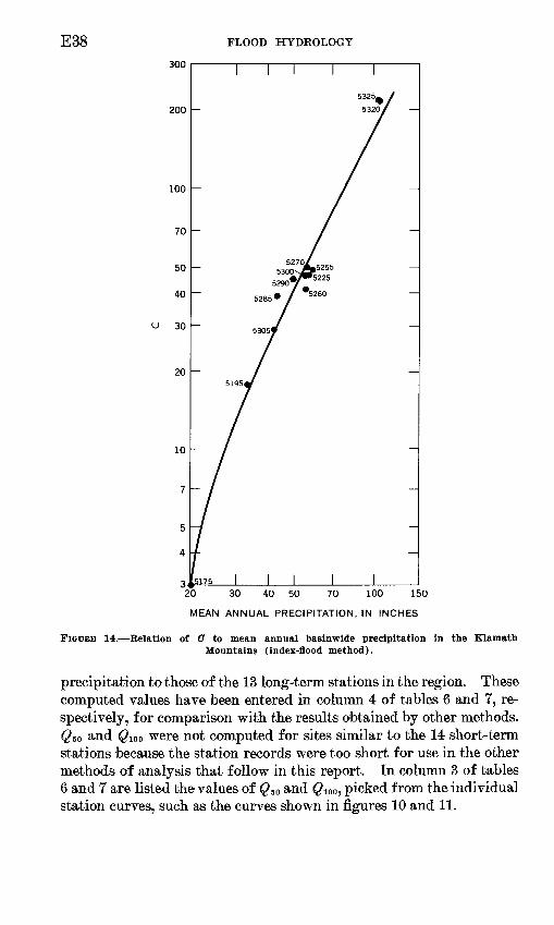
E38 FLOOD HYDROLOGY
300
200 -
100 -
10 -
20 30 40 50 70 100 150
MEAN ANNUAL PRECIPITATION, IN INCHES
FIGURE 14. Relation of G to mean annual basinwide precipitation in the Klamath Mountains (index-flood method).
precipitation to those of the 13 long-term stations in the region. These computed values have been entered in column 4 of tables 6 and 7, re spectively, for comparison with the results obtained by other methods. Qso and QW o were not computed for sites similar to the 14 short-term stations because the station records were too short for use in the other methods of analysis that follow in this report. In column 3 of tables 6 and 7 are listed the values of Q50 and $i00 , picked from the individual station curves, such as the curves shown in figures 10 and 11.

METHODS USED IN FLOOD-FREQUENCY STUDIES, CALIFORNIA E39
"53
Se
<e,"53
-Sft
!
'3-fe'§
2«|
<*5 < a> d wfisls
+ 1 I ' +
+ 1
+ 1
., _,+ 1
sssss
+ 1 ++
I++
03,Q
3!O]_|
SnS q s ia sis
S3 '
2SSSS
I I I I I I I
CO CO * Ofc; «0 10
+777i+ +
fs'sgl^
+ 1 I I I
Ti-J'ia'crf'^iH'ffl'TiJ'oo' (NtcSS^gS
S s a s s| 2

TABL
E 7.
Qio
o fo
r st
ream
s in
nor
th c
oast
al C
alif
orni
a as
det
erm
ined
fro
m g
raph
ical
ly d
eriv
ed f
lood
-fre
quen
cy c
urve
s an
d l>
y va
riou
sm
etho
ds o
f re
gion
al f
lood
-fre
quen
cy a
naly
sis
Inde
x N
o. 1
Sta
tion
2
Qioo
from
gr
aph
ic
ally
- de
rive
d st
atio
n cu
rves
(c
fs)
3
Inde
x-fl
ood
met
hod
Qioo
(c
fs)
4
Per
cent
di
ffer
en
ce
from
co
l. 3
5
Mul
tipl
e co
rrel
atio
n
Qioo
(c
fs)
6
Per
cent
di
ffer
en
ce
from
co
l. 3
7
Log
arith
mic
no
rmal
di
stri
buti
on
Qioo
(c
fs)
8
Per
cent
di
ffer
en
ce
from
co
l. 3
9
Ext
rem
e- va
lue
prob
abil
ity
dist
ribu
tion
Qioo
(c
fs)
10
Per
cent
di
ffer
en
ce
from
co
l. 3
11
Pear
son
type
III
di
stri
buti
on
Qioo
(c
fs)
12
Per
cent
di
ffer
en
ce
from
co
l. 3
13
Gam
ma
dist
ribu
tion
Qioo
(c
fs)
14
Per
cent
di
ffer
en
ce
from
co
l. 3
15
Cal
ifor
nia
Coa
st R
ange
s
4615
4755
47fi5
4770
4785
22,1
0020
,900
170
000
530,
000
43,6
00
23,0
0011
,600
EQO
nnn
49,5
00
+4
_ 44
-32
+10
+14
29,5
0015
,700
545,
000
59,0
00
+3
3-2
5-2
61
0
+35
29,4
00IE
Q
AA
131,
000
560,
000
58,6
00
+3
3-2
4-2
3+
61
QA
25,6
0013
,500
115,
000
535,
000
53,2
00
+16
-35
-32
+1
+22
26,5
0013
,900
no
nnn
554,
000
55,0
00
+20 qq
-30
+5
+26
25,6
00tO
7
AA
111,
000
507,
000
51,5
00
o+
16
<5-3
4
°q.
t"1
-4
o+
18
£j
Kla
mat
h M
ount
ains
5175
5195
5225
5255
5270
5300
5305
5325
6,00
037
,500
QO
K
flfl
76,7
0017
0,00
019
2,00
044
5,00
018
6,00
0
4,28
036
,000
net
nnn
101
000
174,
000
207,
000
431,
000
200,
000
_ O
Q
-4 +16
1 00
1 0
1 ,q
-3 10
8,42
024
,300
76,4
0079
,800
132,
000
220,
000
445,
000
231,
000
-1.4
A-3
5-7 +
4-2
2+
15 0
-1.9
.4
9,70
026
,200
78,6
0081
,800
149,
000
272,
000
695,
000
202,
000
+6
2-3
0 5 +
7-1
2+
42
+5
6 10
6,65
019
,400
61,8
0064
,400
111,
000
193,
000
423,
000
188,
000
+1
1-4
8-2
5-1
6-3
5+
1-5 +1
7,30
021
,200
67,4
0070
,200
122,
000
210,
000
461,
000
204,
000
i n
n
-43 is
_ Q
-28
-L.O
1 A
+1
0
5,95
014
,500
40 5
0041
,900
75,0
0013
4,00
033
5,00
011
0,00
0
-1 -61
-51
-45
-56
-30
-25
-41

METHODS USED IN FLOOD-FREQUENCY STUDIES, CALIFORNIA E41
MULTIPLE CORRELATION
In analyzing the flood magnitude-frequency relation for north coastal California by the multiple-correlation method it was neces sary to eliminate 14 of the 27 gaging stations from consideration because the records for these stations were shorter than 10 years. Of the remaining 13 stations, 5 were in the Coast Ranges and 8 were in the Klamath Mountains. (See table 5.) The fact that so few records were available for study severely handicapped the analysis. Because there were only five stations in the Coast Ranges, no more than one independent variable could be used in a linear correlation, if the correlation were to have any significance at all. Because there were only eight stations in the Klamath Mountains, no more than two independent variables could be used in the correlation.
The first step in the analysis was to obtain the discharges corre sponding to recurrence intervals of 50 years (Q 5o) and 100 years ($100) from the 13 individual station flood-frequency curves. These curves (see, for example, figs. 12 and 13) had been constructed earlier for the index-flood method of analysis. The values of Q 5o and $100 were then correlated with the hydrologic parameters listed in table 5. For the Coast Ranges, drainage area (A) was by far the most signifi cant parameter, and it was used as the sole independent variable in the correlation for the five stations in that physiographic region. Two independent variables drainage area (A) and mean annual basin- wide precipitation (P) were used in the multiple correlation for the eight stations in the Klamath Mountains. Regression equations for $50 and $100 were obtained as follows:
Coast Ranges:(18)(19)
Klamath Mountains:$50 = 0.075 J.o.seepi.965 (20)
^100 =0.128J.°- 842P1 - 912. (21)
For later comparison, the values of Q 50 and $100? computed for the 13 stations by application of these equations, have been entered in column 6 of tables 6 and 7, respectively.
LOGARITHMIC NORMAL DISTRIBUTION
Regional flood-frequency curves for north coastal California were computed by fitting logarithmic normal distributions to the original base data for the 13 stations used in the previous multiple-correlation analysis. The first step in the computation was to convert the natural values of peak discharge to logarithms. The mean and the standard deviation for each station array were then computed. It was neces-

E42 FLOOD HYDROLOGY
sary to adjust the computed mean and the standard deviation for those stations whose peak-discharge records were incomplete for the 28-year base period, 1932-59. The adjustment was accomplished by first correlating concurrent records for each short-term station and a nearby long-term station and then applying equations 3 and 4. At this stage of the computations, the base-period mean (M) and standard deviation ($) were available for all 13 stations.
The values of M and /#, still in logarithmic units, were next region alized by correlation with the hydrologic parameters listed in table 5. In the Coast Ranges region, there was a definite relation between M and drainage area (fig. 15), but S was apparently independent of any measured hydrologic parameters. It was expected that S might vary inversely with mean annual basinwide precipitation, but no correlation was evident. An average value of $=0.235 was therefore used for the Coast Ranges. In the Klamath Mountains, M was found to vary with both drainage area and mean annual basinwide precipitation. No graph has been provided to illustrate the relation, which is expressed by the equation:
M= -2.837 + 0.978,4 + 2.421P, (22) where
M is the base-period mean of the logarithms of annual peak dis charges,
A is the logarithm of the drainage area, andP is the logarithm of the mean annual basinwide precipitation.
CO 5-4UJC3 {£.
I 5.2OCOQ^ 5.0
20.
_l 4.8
D
1 4.6
u. O CO 4.4
I h-
% 4.2
3u. 4.0O
i3.8
I___I200 300 500 1000
DRAINAGE AREA, IN SQUARE MILES
FIGURE 15. .Relation of the mean of the logarithms of annual peak discharges to drainagearea in the Coast Ranges.
METHODS USED IN FLOOD-FREQUENCY STUDIES, CALIFORNIA E43
Values of S in the Klamath Mountains were closely related to mean annual basinwide precipitation as shown graphically in figure 16. By use of these relations, an isohyetal map of mean annual precipitation, and equation 5, a flood-frequency curve can be computed for any site in north coastal California.
By use of the relations just mentioned and equations 12 and 13, values of Q50 and $100, in logarithms, were computed for drainage areas corresponding in size and mean annual basinwide precipitation to those of the 13 long-term gaging stations in the region. The anti- logarithms of Q50 and Qwo have been entered in column 8 of tables 6 and 7, respectively, for later comparison.
EXTREME-VALUE PROBABILITY DISTRIBUTION1 OR GUMBELMETHOD
A regional flood-frequency study of the north coastal region of California was also made by fitting an extreme-value probability dis tribution to the base data for the 13 long-term gaging stations in the region. In this analysis natural values of the discharges were used, not their logarithms. The mean and the standard deviation for each station array were computed, and these two statistics were adjusted for those stations whose peak-discharge records were incomplete for the 28-year base period, 1932-59. To make this adjustment, concurrent records for each short-term station and a nearby long-term station were first correlated, and then equations 3 and 4 were applied. (Note that natural values, and not logarithms, are now used in equations 3 and 4.) After making the adjustment, the base-period mean (M) and standard deviation (S) were available for all 13 stations.
The values of M and S were next regionalized by correlation with the hydrologic parameters listed in table 5. In the Coast Eanges region, both M and /S were related to drainage area (fig. IT). In the Klamath Mountains both M and S were related to drainage area and mean annual basinwide precipitation. No graphs have been provided to illustrate the two multiple relations, which are expressed by the equations:
J/=0.0044d°-944P2 - 164 (23)
S= 0.022 J.°.89ipi.86i? (24) where
M is the base-period mean of annual peak discharges,S is the base-period standard deviation of annual peak dis
charges,A is the drainage area, andP is the mean annual basinwide precipitation.

E44 FLOOD HYDROLOGY
Q 2
z o
T" I
|5255
20 30 40 60 80
MEAN ANNUAL BASINWIDE PRECIPITATION, IN INCHES
FIGURE 16. Relation of the standard deviation of the logarithms of annual peak discharges to mean annual basinwide precipitation in the Klamath Mountains.
300,000
200,000
100,000
80,000
60,000
50,000
40,000
1°* O 30,000
!2 o- 20,000
0 g 10,000Q _o: z 8000
Q
< 6000
W 5000
4770 -\
30 50 100 200 300 500 1000 2000 3000 500C
DRAINAGE AREA, IN SQUARE MILES
FIGURE 17. Relation of the mean and the standard deviation of annual peak discharges to drainage area in the Coast Ranges.

METHODS USED IN FLOOD-FREQUENCY STUDIES, CALIFORNIA E45
By use of the relations expressed in figure 17 and in equations 23, 24, and 6, a flood-frequency curve can be computed for any site in north coastal California.
By use of the foregoing relations and equations 14 and 15, values of Qso and Q1W were computed for drainage areas corresponding in size and mean annual basin wide precipitation to those of the 13 long- term gaging stations in the region. These values are listed in column 10 of tables 6 and 7, respectively, for later comparison.
PEARSON TYPE III DISTRIBUTION
A fifth flood-frequency analysis was made for the north coastal region of California by fitting a Pearson type III distribution to the peak-discharge data for the 13 long-term gaging stations in the region. The computation and regionalization of the base period (M) and standard deviation (8) for this study are identical with those for the Gumbel method of analysis. Consequently, the graphs for the Coast Ranges (fig. 17) and equations 23 and 24 for the Klamath Mountains were applicable for this analysis. The next step was to determine the coefficient of skew for each station. This was done by first using equation 7 to compute the annual peak discharges needed to complete the 28-year array at each short-term station, and then applying equa tion 8 to compute the coefficient of skew (g) for each station. For the streams in the Coast Ranges, the individual values of g ranged from 0.84 to 2.04; for the streams in the Klamath Mountains they ranged from 1.07 to 3.00. In neither region did g correlate with the selected hydrologic parameters. Consequently, the average value of g in each region was assumed to be the regional value of that statistical param eter. Under this assumption the regional value of g for the Coast Ranges is 1.46, and for the Klamath Mountains, 1.83.
By use of the regional relations for M and S as indicated by curves given in figure 17 and equations 23 and 24, the appropriate regional value of <7, table 1, and equation 9, a flood-frequency curve can be computed for any site in the region, whether gaged or ungaged. Val ues of Qso and Q100 were computed by use of the relations and table just mentioned for drainage areas corresponding in size and mean annual basinwide precipitation to those of the 13 long-term gaging stations in the region. These values have been entered in column 12 of tables 6 and 7, respectively, for later comparison with the results obtained by the other methods of analysis.
GAMMA DISTRIBUTION
The gamma distribution was also used to analyze the flood magni tude-frequency relation for streams in north coastal California. A
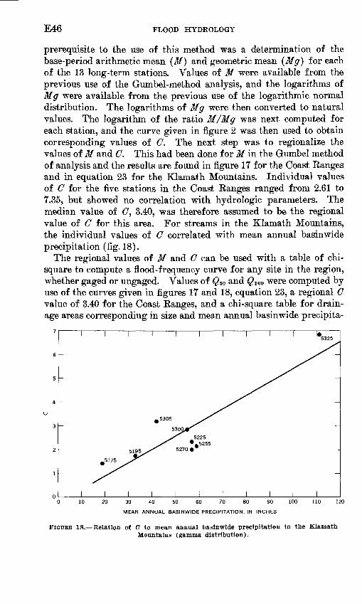
E46 FLOOD HYDROLOGY
prerequisite to the use of this method was a determination of the base-period arithmetic mean (M) and geometric mean (Mg) for each of the 13 long-term stations. Values of M were available from the previous use of the Gumbel-method analysis, and the logarithms of Mg were available from the previous use of the logarithmic normal distribution. The logarithms of Mg were then converted to natural values. The logarithm of the ratio M/Mg was next computed for each station, and the curve given in figure 2 was then used to obtain corresponding values of C. The next step was to regionalize the values of M and C. This had been done for M in the Gumbel method of analysis and the results are found in figure 17 for the Coast Ranges and in equation 23 for the Klamath Mountains. Individual values of C for the five stations in the Coast Eanges ranged from 2.61 to 7.35, but showed no correlation with hydrologic parameters. The median value of £7, 3.40, was therefore assumed to be the regional value of C for this area. For streams in the Klamath Mountains, the individual values of C correlated with mean annual basinwide precipitation (fig. 18).
The regional values of M and C can be used with a table of chi- square to compute a flood-frequency curve for any site in the region, whether gaged or ungaged. Values of Q50 and Q100 were computed by use of the curves given in figures 17 and 18, equation 23, a regional C value of 3.40 for the Coast Eanges, and a chi-square table for drain age areas corresponding in size and mean annual basinwide precipita-
5225 -5255
5270
0 10 20 30 40 50 60 70 80 90 100 110 12
MEAN ANNUAL BASINWIDE PRECIPITATION, IN INCHES
FIGURE 18. .Relation of C to mean annual basinwide precipitation in the Klamath Mountains (gamma distribution).

METHODS USED IN FLOOD-FREQUENCY STUDIES, CALIFORNIA E47
tion to those of the 13 long-term gaging stations in the region. These values are listed in column 14 of tables 6 and 7, respectively, for later comparison with the results obtained by the other five methods of analysis.
DISCUSSION OF RESULTS OF THE ANALYSES
Because of the short period covered by most records of peak dis charge in California, the true values of the 50-year flood (Q50 ) and the 100-year flood ( Qwo ) are not known. Although the peak discharges of the greatest and second greatest floods in the past 100 years can often be deduced within fairly close limits by the use of qualitative historical information, utilization of this information provides, at best, only a single 100-year sample of flood events. This sample may or may not be representative of long-term flood activity. Furthermore, in each of the two California regions studied, the greatest flood in the past 100 years at each station was caused by a single meteorological event. This was generally true, also, of the second greatest flood in the past 100 years. Thus, all stations experienced the same major flood events and, therefore, regionalization of the data has had little effect in re ducing the sampling error that results from having a nonrepresentative sample of floods at a gaging station. We can do nothing about the sampling error, however, and must proceed on the assumption that our sampling of flood events adequately represents the norm of flood ac tivity and that our values of Q50 and Qwo for each station, as deduced with the help of historic information, have only random scatter from their true values.
Tables 3 and 4 present a summary of values of Q50 and $100, respec tively, for streams in the San Diego.area, obtained by various methods of flood-frequency analysis. Similar tabulations for north coastal California are given in tables 6 and 7. Because all methods attempt to fit some relation to the single flood array that is available for each station in a region, it is presumed that the method that fits the observed data best is the most reliable one for use. In this study the values of Q50 and Qwo obtained from the graphically-derived individual station flood-frequency curves (col. 3 in tables 3,4,6, and 7) are considered the standard for judging the reliability of the various methods of analysis. Note that these values of Q50 and Q 100 in column 3 are more than mere extrapolations; they have been determined from a careful assessment of qualitative historical information. Tables 3, 4, 6, and 7 also list the differences, in percent, between the values of Q50 and Qwo as deter mined by each of the six methods of regional flood-frequency analysis, and the values of Q50 and Qwo in column 3. These differences are sum marized in table 8. Ideally, split-sample testing should have been

TABL
E 8
. Su
mm
ary
of d
iffer
ence
s be
twee
n di
scha
rges
det
erm
ined
fro
m g
raph
ical
ly d
eriv
ed f
lood
-fre
quen
cy c
urve
s an
d di
scha
rges
com
pute
d by
var
ious
met
hods
of
regi
onal
flo
od-f
requ
ency
ana
lysi
s
Ran
ge o
f diff
eren
ces
(per
cent
)
Num
ber
of si
tes
with
diff
eren
ces
in in
dica
ted
rang
e
Quo
Inde
x-
flood
m
etho
dM
ultip
le
corr
elat
ion
Log
arith
m
ic n
orm
al
dist
ribu
tion
Ext
rem
e-
valu
e pr
obab
ilit
y di
stri
butio
n
Pear
son
type
III
di
stri
butio
nG
amm
a di
stri
butio
n
Qioo
Inde
x-
flood
m
etho
dM
ultip
le
corr
elat
ion
Log
arith
m
ic n
orm
al
dist
ribu
tion
Ext
rem
e-
valu
e pr
obab
ilit
y di
stri
butio
n
Pear
son
type
III
di
stri
butio
nG
amm
a di
stri
butio
n
San
Die
go a
rea
+ + + + + + + + 0
,151
-222
). _
_,126-150) .--
(101-125) __
__ -_
81-100)- .--
61-8
0)..
- _ .-
21-40).. __ .-
(1-2
0)..
..
(1-20). __
____
__
(21-
40).
---
----
(61-
80).
.
Tota
l ___
___
2 2 5 0 5 4 18
1 2 4 3 5 3 18
1 1 1 4 3 2 3 0 3 18
1 0 2 5 9 1 18
1 1 0 6 8 2 18
2 6 9 1 18
1 1 4 2 0 6 4 18
r
1 1 7 2 4 3 18
5 0 2 3 1 4 1 2
18
1 6 8 3 18
1 1 0 4 4 8 18
1 5 8 4 18

METHODS USED IN FLOOD-FREQUENCY STUDIES, CALIFORNIA E49
COOIN I CO
<NCO I COOCO I (N
COi-4<N I CO
FT
+++
E50 FLOOD HYDROLOGY
used in comparing computed and recorded values of Q50 and Q100. In split-sample testing, half the stations would be used to derive the rela tions necessary to compute Q50 and Qwo, and the remaining stations would be used to compare computed and recorded values. Unfor tunately, there were too few stations to permit split-sample testing, and consequently all stations were used both in the derivation of the relations and in the comparison of Q50 and Qw
It should be pointed out that the percentage differences listed in table 8 do not, in themselves, give a complete picture of the relative reliability of the various methods; another factor is the number of degrees of freedom lost in each analysis. The details of this loss will not be discussed. Suffice it to say that the index-flood method, as used in the analysis for north coastal California, has more lost degrees of freedom than the other methods because of the numerous areal sub divisions that were established for the region. Consequently, the results obtained in north coastal California by this method have some what less statistical significance than those obtained by the other five methods.
Table 8 shows that all methods of analysis gave better results for north coastal California than for the San Diego area. This is to be expected because the San Diego area, being generally subhumid, has highly variable streamflow, and it is almost axiomatic that the more variable the streamflow, the more difficult it is to make a reliable deter mination of the flood magnitude-frequency relation. The difficulty is compounded when the period of record is short. A comparative meas ure of the variability of an array of data is the coefficient of variation, which is defined as the ratio of the standard deviation of the array to its mean, or S/M. The greater variability of the San Diego area streams is shown by the fact that the coefficient of variation for these streams ranged from 1.5 to 2.8, whereas in the north coastal area the range was from OA to 1.1.
Table 8 shows that for the San Diego area the two empirical meth ods the index-flood method and multiple correlation gave results that are in much closer agreement with the "standard" values of Q50 and $100 than are the values obtained by any of the four methods using statistical distributions. This agreement is not surprising because the two empirical methods are the only ones that made use of the qualita tive historical data that were available, and it is on these data that the standard values of Q50 and Qwo are based. In effect, the period of observed data for the two empirical methods was 100 years or more, as opposed to the much shorter period of observed data used with the other four methods. For the north coastal area, the difference in the quality of results between the two empirical methods and the methods using statistical distributions is less pronounced. The gamma distri-

METHODS USED IN FLOOD-FREQUENCY STUDIES, CALIFORNIA E51
bution gave the poorest results, but of the other five methods, no single method was outstandingly superior. The implication is that in a humid area where all streams are subject to the same general storms, most methods of analysis will give satisfactory results.
INDEX-FLOOD AND MULTIPLE-CORRELATION METHODS
The multiple-correlation method is superior to the index-flood method, particularly in subhumid areas. Not only did the multiple- correlation method give generally better results in this study, as in dicated in table 8, but it has a more rational basis than the index-flood method. The weakness of the index-flood method is that it assumes that the slopes of the flood-frequency curves for the streams in a given region vary randomly from some median value. The Geological Sur- very test for homogeneity of slope in a region has some serious short comings and often indicates homogeneity of slope where none exists (Benson, 1962, p. 21). Actually, there are many physiographic and climatologic factors that affect the slope of the flood-frequency curve, and it is often a matter of fortuity that the curves for all streams in a region have similar slopes. In several previous studies the delinea tion of the boundaries of regions of homogeneous slope, based on the homogeneity test, has resulted in maps that resemble political gerry manders. The index-flood method can be used to advantage, however, for a region where there are insufficient stations with 10 or more years of record to permit a significant multiple correlation to be made. In addition, those records that are shorter than 10 years are helpful in defining the regional relation for the mean annual flood ($2.33)-
STATISTICAL DISTRIBUTIONS
We turn our attention now to the four methods of analysis that are based on statistical distributions logarithmic normal, extreme-value probability, Pearson type III, and gamma. As already mentioned, these methods are empirical in the sense that one of the four distribu tions must be arbitrarily selected for use. However, once a distribu tion has been selected, the analysis becomes strictly objective. Because these methods did not make use of the available historical information, the results obtained from their application were not as satisfactory as those obtained by use of either the index-flood or multiple-correlation methods. This was particularly true in the subhumid San Diego area. If the high-water ends of these distributions had been later modified on the basis of the historical information, as is often done, the results would have been more satisfactory, but there would then have been little point in using one of the theoretical distributions. The all-im portant high-water end of the flood magnitude-frequency relation
E52 FLOOD HYDROLOGY
would no longer be controlled by the statistics of the selected distribu tion, but would depend on the judgment of the analyst in interpreting the historical information and assigning probabilities to the peak dis charges. Table 8 shows that the logarithmic normal distribution gave results that were generally high; the other three distributions gave results that tended to be low. The logarithmic normal distribu tion also had a greater spread of differences from the standard values of Q5 o and Q10o than did the other three distributions. It is not to be inferred, however, that this is a general rule. It is of interest that the flood-frequency handbook used by the U.S. Army, Corps of Engineers, which recommends the logarithmic normal distribution method, cau tions against its use in subhumid areas (Beard, 1962, p. 22).
Tables 3, 4, 6, and 7 show that the four statistical distributions, when applied to the same peak-discharge data, gave widely differing results for individual stations. These distributions have all been ex tensively used elsewhere and each has the support of reputable stat- istician-hydrologists as being the distribution that best describes the occurrence of flood events. Obviously all methods cannot be best, and the inescapable conclusion is either that the true distribution that de scribes the occurrence of flood events is not known or that no single distribution is best for all of the many widely varying hydrologic con ditions found in a country as large as the United States. In the United States most of the long-term discharge records are for large streams draining humid areas, and it is these records that have been used in the past to test the adequacy of the various distributions. In this study we have seen that in a humid area all methods give results that are generally satisfactory. Therefore, it is not surprising that each distribution has strong proponents among hydrologists. Examina tion of the various distributions shows that within the range of prob abilities usually used in flood-frequency studies, the extreme-value probability distribution may be considered a special case of the Pear- son type III distribution, one in which the coefficient of skew is 1.14. The gamma distribution is likewise a special case of the Pearson type III distribution, one in which the locus parameter is zero.
From the preceding paragraph, it would appear that the most de sirable distribution for use would be the one that is most flexible and can therefore fit the peak-flow data closest. Of the four distributions studied, the Pearson type III distribution is the least rigid because the Pearson type III distribution uses three statistical parameters, whereas the other three distributions use two parameters, with the third

METHODS USED IN FLOOD-FREQUENCY STUDIES, CALIFORNIA E53
parameter either constant or determined by one or both of the others. We know too little of the laws governing the occurrence of flood events to hazard a guess concerning the value of the third parameter, and it therefore seems reasonable to use a general or flexible distribution, such as the Pearson type III, rather than some rigid distribution, such as one of the other three, which has a built-in restriction on the value of the third parameter.
If we exclude the two empirical methods and confine our comparison of results to the four statistical distributions, we should concern our selves only with the values of Q50 and not $100- In this study, the values obtained for Q50 result primarily from the distribution of peak dis charges during the base periods; they are not seriously affected by the consideration of qualitative historical data, as are the values of $100- Examination of the percent differences for Q50 in table 8 shows that the Pearson type III distribution fitted the array of observed data better than any of the other three statistical distributions.
The principal objection to the use of Pearson type III distribution has been the fact that the skew statistic, which is used in the distri bution, has a large standard error when there are relatively few items in the array of peak discharges. It has been claimed that under these circumstances the coefficient of skew has little or no significance. Whether or not the coefficient of skew computed for an isolated station is statistically significant may be debatable, but it seems reasonable to accept as significant a regionalized value of the coefficient based on numerous station records, even though the records may not be entirely independent.
Because regionalization of the statistics for the individual station arrays might have obscured the relative abilities of the four distribu tions to fit the station data, the individual statistics for each station array were used to compute individual stition flood-frequency curves. The computed value of Q50 from each of these curves was compared with the "standard" values of Q50 listed in column 3 of tables 3, 4, 6, and 7. The comparison is summarized in table 9. The Pearson type III distribution gave results that were superior to those obtained by use of the other three distributions.
Although this comparison study of flood-frequency methods was based on small samples 18 stations in southwest California and 13 stations in northwest California the results and conclusions appear to be meaningful because they can be explained rationally.

E54 FLOOD HYDROLOGY
TABLE 9. Summary of differences between Qso determined from graphically derived flood-frequency curves and Q50 computed from various distributions using statistical parameters from individual station arrays
Range of differences (percent)
Number of sites with differences in indicated range
Logarithmic normal dis tribution
Extreme-value probability distribution
Pearson type III distribu
tion
Gamma distribution
San Diego area
+ (121-373). __ __. __ _______+ (101-120)___-_____ _ _______+ (81-100)________ ____________+ (61-80)_____-----___________+ (41-60)-____----____________+ (21-40). _.__-._________.____
+ (1-20)_____ _________________0____-__- _ _._.-(1-20)______ ________________
-(21-40)_____________________-(41-60).... _ ______ _ _____-(61-84). ____________________
Total... ___ _ ____ __
320241
004
011
18
100
001862
18
10000
106
712
18
10
002
672
18
North coastal area
+ (31-34)________. ____________+ (21-30)_____._______________+ (11-20). ____________________
+ (1-10)__. ___________________0__ _________________________-(1-10)...... __....__..._..._
-(11-20)... __________________-(21-26)_--_------.__________
Total._________ ______ _
103
503
1
13
10
11
1
13
804
01
13
05
71
13
SUMMARY AND CONCLUSIONS
Regional flood-frequency studies were made by six different meth ods for the subhumid San Diego area in southwestern California and for the humid coastal area in northwestern California. A 55-year base period was used for 18 peak-discharge records in the San Diego area; a 28-year base period was used for 13 peak discharge records in north coastal California. All flood-frequency curves were extrap olated to the discharges corresponding to the 50-year recurrence in terval ($50) and to the 100-year recurrence interval ($100) Two of the six methods of analysis the index-flood and multiple-corre lation methods are to some extent empirical and permit the analyst

METHODS USED IN FLOOD-FREQUENCY STUDIES, CALIFORNIA E55
to use whatever qualitative or historical information is available for extrapolating the flood-frequency relation. The other four methods are based on statistical distributions the logarithmic normal, ex treme-value probability, Pearson type III, and gamma distributions. These four methods are empirical in the sense that one of the distri butions is arbitrarily selected for use; but once selected, the analysis becomes strictly objective and the extrapolation is automatically made from a determination of the statistics of the array of peak discharges.
There is a lack of agreement among hydrologists as to which method or which distribution is the most reliable for defining the flood magni tude-frequency relation at a site. The purpose of this study was to compare the results obtained by applying each of the six methods of analysis to the basic data and to appraise the relative reliability of the methods. The magnitude of the greatest and second greatest flood peaks in the past 100 years in the two study areas were generally known within reasonable limits of accuracy, and with this knowledge it was possible to derive values of Q5n and Qwo for each gaging station that are representative of flood activity during the past century. These values of Q50 and $10 o were used as standards for the com parison and appraisal of the methods of analysis.
It was concluded that all methods of analysis give better results in a humid region, such as north coastal California, than in a sub- humid region, such as the San Diego area, because streamflow is usually less variable in a humid region.
A decision as to the preferred method of flood-frequency analysis depends on whether or not historical data, either quantitative or qualitative, are available concerning the magnitude of floods that oc curred in the years prior to the collection of streamflow records. If such information is available, the empirical methods the index-flood and multiple-correlation methods are superior to any of the four methods using statistical distributions owing to the fact that only the empirical methods use historical data, and use of these data gives a longer time base for the analysis. In this study, our knowledge of the magnitude of the greatest and second greatest flood peaks in the past 100 years extended the period of observed data, in effect, to 100 years or more for the empirical methods. This is a much longer period than the base periods that were used with the other four methods of analysis. Of the two empirical methods, the multiple-regression method is superior because it has a much more rational basis than the index-flood method and in addition gives better results.
Where the peak-discharge data are limited entirely to the period during which streamflow records were collected (no historical data available), a method based on the distribution of the array of peak flows is preferred because of its greater objectivity. Of the four dis-

E56 FLOOD HYDROLOGY
tributions tested, the Pearson type III is the most desirable. It is more flexible than the other three and will generally fit the peak-dis charge data best because the Pearson type III distribution is a three- parameter distribution with no built-in restriction on the value of the third, or skew, parameter. The other distributions are two-parameter distributions with an implied constant value for the third parameter. Objection to the Pearson type III distribution has been based on the large standard error of the coefficient of skew, but this objection can be overcome by using a regional value of the coefficient based on numerous station records.
Although this comparison study of flood-frequency methods was based on small samples from only one part of the United States, the results and conclusions appear to be meaningful because they can be explained rationally.
REFERENCES CITED
Alexander, G. N., 1962, The use of the gamma distribution in estimating regu lated output from storages: Australian Inst. of Engineers, Civil Engineers Trans., v. CE 4, no. 1, p. 29-34.
Arkin, Herbert and Colton, R. R., 1950, Tables for statisticians: New York, Barnes & Noble, 152 p.
Beard, L. R., 1962, Statistical methods in hydrology: U.S. Army Corps of Engi neers, Civil Works Investigations Project CW-151, 62 p.
Benson, M. A., 1962, Evolution of methods for evaluating the occurrence of floods: U.S. Geol. Survey Water-Supply Paper 1580-A, 30 p.
California Department of Water Resources, 1963, Flood hazard investigation, San Diego County: Bull. 112, app. A, 78 p.
Dalrymple, Tate, 1960, Flood-frequency analyses: U.S. Geol. Survey Water- Supply Paper 1543-A, 80 p.
Elderton, W. P., 1953, Frequency curves and correlation; Washington, Harren Press, 272 p.
Ezekiel, Mordecai and Fox, K. A., 1959, Methods of correlation and regression analysis: New York, John Wiley & Sons, 548 p.
Fenneman, N. M.. 1931, Physiography of western United States: New York, McGraw-Hill Book Co., 534 p.
1938, Physiography of eastern United States: New York, McGraw-Hill Book Co., 714 p.
Gumbel, E. J., 1958, Statistics of extremes: New York, Columbia Univ. Press, 375 p.
Jarvis, C. S., and others, 1936, Floods in the United States, magnitude and fre quency: U.S. Geol. Survey Water-Supply Paper 771, 497 p.
Potter, W. D., 1961, Peak rates of runoff from small watersheds: U.S. Bur. Public Roads, Hydraulic Design Series No. 2, 35 p.
Rantz, S. E., 1964, Surface-water hydrology of coastal basins of ^northern Cali fornia : U.S. Geol. Survey Water-Supply Paper 1758, 77 p.
Thorn, H. C. S., 1958, A note on the gamma distribution: Monthly Weather Rev., v. 86, no. 4, p. 117-122.
o

Flood Hydrology
GEOLOGICAL SURVEY WATER-SUPPLY PAPER 1580
This volume was published as separate chapters A-E
UNITED STATES DEPARTMENT OF THE INTERIOR
STEWART L. UDALL, Secretary
GEOLOGICAL SURVEY
Thomas B. Nolan, Director
CONTENTS
[Letters designate the separately published chapters]
(A) Evolution of methods for evaluating the occurrence of floods, by Manuel A. Benson.
(B) Factors influencing the occurrence of floods in a humid region of diverse terrain, by Manuel A. Benson.
(C) Effect of reservoir storage on peak flow, by William D. Mitchell.(D) Factors affecting the occurrence of floods in the Southwest, by M. A. Benson. (E) A comparison of methods used in flood-frequency studies for coastal basins
in California, by R. W. Gruff and S. E. Rantz.