a comparison of local and wide area differential corrections disseminated using ... · corrections...

A COMPARISON OF LOCAL AND WIDE AREA GNSS

DIFFERENTIAL CORRECTIONS DISSEMINATED USING THE NETWORK TRANSPORT OF

RTCM VIA INTERNET PROTOCOL (NTRIP)

GEORGE MCKESSOCK

April 2007

TECHNICAL REPORT NO. 249

A COMPARISON OF LOCAL AND WIDE AREA

GNSS DIFFERENTIAL CORRECTIONS DISSEMINATED USING THE NETWORK

TRANSORT OF RTCM VIA INTERNET PROTOCOL (NTRIP)

George McKessock

Department of Geodesy and Geomatics Engineering University of New Brunswick

P.O. Box 4400 Fredericton, N.B.

Canada E3B 5A3

April 2007

© George McKessock 2007

PREFACE

This technical report is a reproduction of an undergraduate senior technical report

submitted in partial fulfillment of the requirements for the degree of Bachelor in Science

in Engineering in the Department of Geodesy and Geomatics Engineering, April 2007.

The research was supervised by Dr. Richard Langley and was supported by Cansel

Survey Equipment Inc. and Bundesamt für Kartographie und Geodäsie (BKG)

As with any copyrighted material, permission to reprint or quote extensively from this

report must be received from the author. The citation to this work should appear as

follows:

McKessock, G. (2007). A Comparison of Local and Wide Area GNSS Differential

Corrections Disseminated using the Network Transport of RTCM via Internet Protocol (NTRIP). Senior technical report, Department of Geodesy and Geomatics Engineering Technical Report No. 249, University of New Brunswick, Fredericton, New Brunswick, Canada, 66 pp.

Abstract

Psuedorange corrections (PRCs) have long been used to improve the accuracy of

GNSS solutions in real time. Today, they continue to be useful for sub-metre level

requirements, such as when setting ground control for satellite imagery and for en route

navigation on land, in the air and at sea. The transmission of these corrections has

traditionally been facilitated using either radio or satellite communications. The

Networked Transport of RTCM via Internet Protocol (NTRIP) specification takes

advantage of the availability of Internet over digital mobile phones to disseminate PRCs.

In this report, NTRIP has been used to transmit both localized wide area and local

PRC corrections over the Internet to a client receiver where they have been applied. The

accuracy of different solutions is compared. In addition, the convergence of different

solutions is analyzed. This analysis will enable potential users to determine the position

and height accuracy that they can expect to achieve under various scenarios as well as the

observation times which they should employ.

Results for horizontal positions showed errors at a 95% confidence level to be at

the 2-metre level for uncorrected GNSS, 30 cm for GNSS augmented with local

corrections generated at UNB and 1.0 m for corrections generated 430 km away. The

Canadawide Differential GPS (CDGPS) wide area system produced errors of 60 cm.

Results for heights were of a similar order. However, we found that height

solutions were significantly more correlated with observation time than were horizontal

positions.

Abstract Page: ii

Our work showed that NTRIP could be used easily to both disseminate and use

localized wide area and local differential corrections. We believe that as costs for digital

mobile service becomes cheaper and more widely available, NTRIP will become

commonly used.

In addition, we recommend that the CDGPS service consider supporting NTRIP.

Currently, CDGPS has a limited user-base because it is accessible only with the use of

receivers containing NovAtel®-based chipsets. We believe that NTRIP can potentially

bring CDGPS to a much wider object.

Finally, by far, the best position and height accuracies achieved were with the use

of local differential corrections. Even when the reference receiver was 430 km from the

user receiver, resulting solutions were better in both accuracy and precision than

uncorrected solutions. Canada and New Brunswick each operate an Active Control

Network, consisting of many continuously operating GNSS receivers that are already

connected to the Internet. We believe that with very little effort, this network can be

extended, using NTRIP, to disseminate DGNSS corrections.

Abstract Page: iii

Acknowledgements

I would like to thank the following people for their help with this project:

Dr. Richard Langley, Department of Geodesy and Geomatics at UNB, Fredericton.

Dr. Langley suggested this topic and provided significant support along the way. He provided help with equipment setup, advice and his door was always open. I very much appreciate that he took time to oversee this project!

Mike Wolfe, BScE (UNB, GGE), MScF (UNB, Forestry), GPS Infrastructure Engineer, CanSel®

Mike provided help from the initial conception of this project. Through CanSel®

he provided equipment and software including a Trimble® NetR5 reference station, a Trimble® GeoXT mapping-grade GPS receiver, a GSM mobile phone with service and software to interface with the GeoXT. Mike also configured the equipment for me, showed me how to use it and answered many questions.

Christian Waese, EUREF-IP & IGS-IP Team, BKG, Germany Mr. Waese, in association with George Weber and Denise Dettmering, provided

us with mountpoints on the BKG NTRIP caster. Without this help, I would likely have been unable to carry out the CDGPS portion of this work.

Rodrigo Leandro, PhD student, Department of Geodesy and Geomatics, UNB, Fredericton

Rodrigo configured and maintained the Trimble® NetR5 receiver at UNB. He

also provided the “known” coordinates for our antenna.

Sandi McKessock Sandi proofread the draft of this report. Any remaining errors are my own.

Acknowledgements Page: iv

Table of Contents

Abstract ............................................................................................................................... ii Acknowledgements............................................................................................................ iv Table of Contents.................................................................................................................v Table of Figures ................................................................................................................ vii Table of Abbreviations .................................................................................................... viii 1.0 INTRODUCTION .........................................................................................................1 2.0 DIFFERENTIAL GNSS AND STANDARDS .............................................................5

2.1 Pseudorange Corrections .........................................................................................5 2.1.1 Determination of user position using GNSS...................................................5

2.2 DGNSS Sources of Error .........................................................................................9 2.2.1 Sources of Error ..............................................................................................9

2.2.1.1 Satellite clock error .............................................................................9 2.2.1.2 Satellite ephemeris error ...................................................................10 2.2.1.3 Ionospheric Refraction Error ............................................................11 2.2.1.4 Tropospheric Refraction Error..........................................................12 2.2.1.5 Multipath Error .................................................................................13 2.2.1.6 Code, Antenna and Electronic Noise Errors .....................................14

2.2.2 Range Rate Corrections ................................................................................15 2.2.3 Spatial Correlation ........................................................................................16 2.2.4 Temporal Correlation....................................................................................18

2.3 Wide Area versus Local DGNSS...........................................................................19 2.3.1 Wide Area DGNSS (Vector) ........................................................................19

2.3.1.1 RTCA Specification..........................................................................21 2.3.2 Local-Area/Regional DGNSS (Scalar) .........................................................22

2.3.2.1 RTCM Specification .........................................................................22 3.0 THE NTRIP STANDARD ..........................................................................................23

3.1 Overview................................................................................................................23 3.2 NTRIP Sources ......................................................................................................24 3.3 The NTRIP Server .................................................................................................24 3.4 The NTRIP Caster..................................................................................................25 3.5 The NTRIP Client ..................................................................................................26 3.8 NTRIP Administration...........................................................................................26 3.9 Currently Available Resources ..............................................................................27

Table of Contents Page: v

4.0 DATA COLLECTION AND ANALYSIS..................................................................28 4.1 The NTRIP Caster..................................................................................................28 4.2 Setup of NTRIP Servers and Sources ....................................................................29

4.2.1 The CanSel® Caster .....................................................................................29 4.2.2 The BKG Caster............................................................................................29 4.2.3 CDGPS Issues Encountered..........................................................................33

4.2.3.1 ePing Receivers Are No Longer Manufactured................................33 4.2.3.2 Intermittent Problems Encountered with the ePing receiver ............34

4.3 Data Collection Procedures....................................................................................34 4.3.1 GNSS Receiver Selection .............................................................................34 4.3.2 Collecting Data with the Trimble® GeoXT .................................................35

4.3.2.1 Establishing A Bluetooh® “Bond” With a GSM Mobile Phone......35 4.3.2.2 Configuring COM ports for NMEA .................................................37 4.3.2.3 Configuring the NTRIP client...........................................................37 4.3.2.4 Starting data collection. ....................................................................38 4.3.2.5 Capturing NMEA with Hyperterminal® ..........................................39 4.3.2.6 Problems Encountered with the Trimble® GeoXT ..........................39

4.4 Solution Comparisons............................................................................................40 4.4.1 Datum Changes.............................................................................................41 4.4.2 Conversion From Degrees To Metres...........................................................42 4.4.3 2D Position Scatter Plot ................................................................................43 4.4.4 Height Time Series Plot ................................................................................47

4.5 Precision Versus Observation Time.......................................................................49 4.5.1 Horizontal Positioning ..................................................................................50 4.5.2 Height Positioning ........................................................................................52

4.6 Latency Comparisons.............................................................................................53 5.0 CONCLUSIONS..........................................................................................................58

5.1 NTRIP....................................................................................................................58 5.2 CDGPS...................................................................................................................59 5.3 Local DGPS ...........................................................................................................61

References..........................................................................................................................63 Selected Bibliography........................................................................................................67

Table of Contents Page: vi

Table of Figures

2.1.1 Determining position through trilateration ................................................................5 2.2.1 Spatial Correlation of Errors....................................................................................17 3.1.1 The parts of an NTRIP system.................................................................................23 4.2.1 NTRIP server main screen. ......................................................................................30 4.2.2 NTRIP server TCP/IP input configuration screen. ..................................................31 4.2.3 NTRIP server NTRIP caster output configuration screen. ......................................31 4.2.4 A CDGPS Receiver which receives CDGPS modified RTCA corrections and

optionally converts them to RTCM v2.3 corrections ...............................................32 4.2.5 NTRIP server COM input configuration screen for ePing Receiver. ......................32 4.2.6 NTRIP server NTRIP caster output configuration screen for CDGPS corrections.32 4.3.1 The Trimble® GeoXT Series Handheld ..................................................................35 4.4.1 Output of the TRNOBS 3D coordinate transformation program.............................42 4.4.2 2D position solutions with uncertainties at 95% confidence. ..................................44 4.4.3 Ellipsoid height solutions with uncertainties at 95% confidence. ...........................48 4.5.1 Moving average-window algorithm used to compare uncertainty with collection

time. ..........................................................................................................................49 4.5.2 2D position uncertainties versus observation time at 95% confidence....................50 4.5.3 Height uncertainties at 95% confidence. .................................................................52 4.6.2 Latency comparison of differential corrections. .......................................................54 4.6.2 Correlation of CDGPS 2DRMS with correction latency..........................................55 4.6.3 Close-up of correlation of CDGPS 2DRMS with correction latency at a correction

outage........................................................................................................................57

Table of Figures Page: vii

Table of Abbreviations

ACN Active Control Network BKG Bundesamt für Kartographie und Geodäsie

(The German Federal Agency of Cartography and Geodesy) CDGPS Canada-wide Differential GPS CSRS Canadian Spatial Reference System DGNSS Differential Global Navigation Satellite System DGPS Differential Global Positioning System € Currency of the European Union (the “Euro”) EGNOS European Geostationary Navigation Overlay Service FAA Federal Aviation Administration GEO Geostationary Satellite GNSS Global Navigation Satellite System GPS Global Positioning System GPS*C The approach used by CDGPS to compute differential corrections. GSM Global System for Mobile Communications HTTP Hypertext Transfer Protocol IP Internet Protocol ITRF International Terrestrial Reference Frame MRTCA A modified version of RTCA/DO-229 protocol used by CDGPS to

encapsulate vector differential corrections NABU Notice Advisory to Broadcast Users NAD83 North American Datum of 1983 NMEA National Marine Electronics Association NRCan Natural Resources Canada NTRIP Networked Transport of RTCM via Internet Protocol PPP Precise Point Positioning PRC Pseudorange Correction RINEX Receiver Independent Exchange Format RRC Range-Rate Correction RTCM Radio Technical Commission For Maritime Services RTK Real-Time Kinematic SNB Service New Brunswick TCP/IP Transport Control Protocol / Internet Protocol TEC Total Electron Content UNB University of New Brunswick UNBF University of New Brunswick at Fredericton WAAS Wide Area Augmentation System WGS-84 World Geodetic System

Table of Acronyms Page: viii

CHAPTER 1 1.0 INTRODUCTION

A vast range of techniques enables users to obtain point positions using a Global

Navigation Satellite System (GNSS) at various levels of accuracy. At one end of the

spectrum lies code-based autonomous GNSS yielding accuracies in the range of several

metres, while at the other end lies dual-frequency phase post-processed static solutions

yielding accuracies of a few millimeters. Somewhere in the middle lie techniques of

pseudorange correction (PRC) often called “differential correction”. Accompanying each

technique is a cost in both time and dollars. A cheap handheld GPS unit can compute

autonomous solutions in real time for a cost of less than two hundred dollars, while static

solutions might require equipment costing tens of thousands of dollars with solutions

only becoming available after-the-fact.

In this report, accuracy will be defined as the bias, or difference, of an observed

position from a known position. For horizontal positions this bias will be the horizontal

RMS distance of an observation from its known position. For vertical positions, the

height observed above the known position will be used. Uncertainty, or precision, will be

defined as the difference between the observed value and the mean of all observed

values. In addition, all uncertainties will be presented at a 95% confidence level. Thus,

the uncertainty presented is the value inside which 95% of all observations lie. A

statement that a position was measured at mm 8.12.1 ± means that the mean difference

between the observed value and the known value was 1.2m while the 95% of the

observations lie within 1.8m of the mean position of all observations in the data set.

Chapter 1: Introduction Page: 1

Differential corrections are often used to improve autonomous GNSS positions.

The resulting combination is known as differential GNSS* (DGNSS). Pseudorange

corrections (PRCs), to be employed in this report, generally produce horizontal

accuracies in the 0.5m to 2.0m range and can be applied to either code or phase

measurements. Real Time Kinematic (RTK) methods can result in accuracies in the

centimetre range but can only be used in conjunction with phase measurements.

Although less accurate than RTK, PRCs still occupy a solid position in the

modern GNSS market because of their relative low cost and ease of use when compared

to RTK. Applications that are appropriate for these corrections are in establishing ground

control for satellite imagery, providing positioning information for hydrographic surveys,

and providing en route positioning for land, ocean and aerial navigation.

Pseudorange corrections can be broken down into two broad categories: wide

area and regional. Typical examples of wide area DGNSS systems are WAAS (Wide

Area Augmentation System) and CDGPS (Canada-wide Differential GPS). As the name

implies, wide area systems are intended to cover large regions such as all states of the

U.S.A, as in the WAAS case, and most of Canada, as in the CDGPS case. Regional

systems are intended for use in a specific region, such as within the vicinity of a city or

airport. In general, local corrections provide better accuracy than wide area corrections.

* The term DGPS (differential global positioning system) is in common use. However, this term

specifically applies to the United States’ GPS system. Since there are now other systems worldwide, such

as Russia’s GLONASS and the European Union’s Galileo system (which is currently under development),

the more generic term DGNSS will be used here since differential techniques apply to all systems.


For DGNSS corrections to be applied in real time, they must first be computed

and then transmitted to the roving GNSS receiver. Both WAAS and CDGPS use

geostationary satellites (GEOs) to broadcast corrections to users. This may cause

significant problems for some terrestrial users since GEOs can be low on the horizon in

northern latitudes, such as Fredericton, causing the signals to be blocked by terrain and

buildings. For example, GEO-based signals were unavailable for 51.8% of the positions

computed during a 6100 km course driven in Finland (>60ºN) [Chen and Li, 2004].

Due to the wide availability of digital mobile phone availability in both North

America and Europe, this technology has recently come under close scrutiny as a viable

transmission medium for differential corrections. The German Federal Agency of

Cartography and Geodesy has defined and implemented a method of employing the

Hypertext Transport Protocol (HTTP) to disseminate DGNSS corrections via an Internet

Protocol (IP) connection [Weber, 2005]. To accomplish this, they have devised a client-

server model; chosen the Radio Technical Commission For Maritime Service (RTCM)

standard [RTCM, 2001] as a correction format (allowing both PRC and RTK-type

corrections); and devised syntax to extend the ubiquitous HTTP protocol. This model is

known as Network Transport of RTCM via Internet Protocol (NTRIP). In experiments

carried out by Chen and Li, it was found that NTRIP-delivered differential corrections

were available for 98.6% of the position solutions during a 6100km course driven in

Finland (>60ºN).

For the work described in this report, both local and localized wide area

pseudorange corrections were disseminated using NTRIP. The accuracy and

convergence of position and height solutions was analyzed. In addition, some


consideration is given to the latency of corrections since they must travel through the

Internet in a manner that is not under the control of either the purveyor of the DGNSS

corrections or the end user.

Chapter 2 provides background information on DGNSS. Pseudorange corrections

are discussed, as are errors expected and their correlation with the distance between user

and reference station. Chapter 3 provides background information on the NTRIP

specification. Each component of the model is discussed so that the reader can become

familiarized with a technology that will likely become prevalent in the near future.

Chapter 4 discusses the procedures followed when collecting data, as well as

computational procedures and results obtained. Chapter 5 contains conclusions and

recommendations for future work.


CHAPTER 2 2.0 DIFFERENTIAL GNSS AND STANDARDS

2.1 Pseudorange Corrections

2.1.1 Determination of user position using GNSS

Trilateration is a technique used to determine position through the measurement

of ranges. As shown in Figure 2.1.1, a user measures the distance between himself and

several reference stations whose coordinates are known.

ρ1

ρ3

ρ2

Figure 2.1.1: Determining position through trilateration.

Mathematically, each range is represented by the following equation:

( ) ( ) ( )222 zzyyxx iiii −+−+−=ρ (2.1)

Chapter 2: Differential DGNSS and Standards Page: 5

Where: iρ Is the distance observed between the user and a reference

station whose coordinates are known. zyx ,, Are the coordinates of the user in some Cartesian coordinate

system. iii zyx ,,

Are the coordinates of a reference station.

Equation (2.1) fits nicely into a parametric least squares paradigm, with:

a) Three unknowns – the coordinates of the user position

b) One observation – the distance between the user and the reference station, and

c) Three constants – the coordinates of the reference station.

Obviously, with only one observation and three unknowns, the user position cannot be

uniquely determined. For each additional observation, no new unknowns are added.

Hence, by adding observations to two additional reference stations, a unique solution can

be obtained. Adding still more observations results in redundancies that allow

uncertainties to be estimated.

This technique can be used to compute a user position from orbiting satellites.

Each satellite continuously broadcasts a signal at a well-known frequency. Modulated on

the signal is a coded message that contains information including: the location of the

satellite, the time at which the message was sent, and orbital parameters for all satellites.

The receiver can determine which satellite is being observed by means of a pseudo-

random number (PRN) that is used to decode messages, and that uniquely identifies each

satellite. Upon receiving and decoding this message, the user can determine the length of

time that the signal took to travel from the satellite to the user. Using the speed of light in

a vacuum, the range to the satellite can be approximated. Since this range contains

significant error it is called the pseudorange.


Pseudorange observations are commonly modeled as follows [Misra and Enge,

2001]:

( ) iiiiii TIdTdtcr ερ +++−+= (2.2)

Where: iρ Is the observed range between the user and satellite ‘i’.

ir Is the geometric range between the user and the satellite (shown in equation 2-1).

c Is the speed of light in a vacuum. dt Is the difference between the user’s receiver’s clock and true

GNSS time. idT

Is the difference between the satellite’s clock and true GNSS time.

iI Is extra effective distance traveled by the satellite signal due to refraction in the ionosphere.

iT Is the extra effective distance traveled by the satellite signal due to the troposphere.

iε Represents any terms not modeled, such as noise caused by the receiver’s electronics and multipath.

In order to employ a parametric least squares approach to equation (2.2), it is

necessary to somehow deal with the clock and atmosphere terms. The general

prescription is to:

a) Treat receiver clock error as an unknown parameter and solve for it.

b) Use parameters encoded in the GNSS signal to approximate satellite clock error

and model the ionosphere.

c) Model the troposphere based on approximate location and time of day and year.

Using this approach, it is typically possible to achieve a position accuracy of 10 metres at

95% confidence in most situations [RTCM, 2001].

While this level of accuracy may be quite acceptable for en route navigation in

open seas or aloft, it is generally not sufficient for applications such as runway approach

or in-harbour navigation [RTCM, 2001]. In an attempt to improve accuracy, researchers


have developed a considerable number of approaches. The central method considered in

this report is that of differential correction using pseudoranges.

Under this method, a “reference” GNSS receiver is placed at a location whose

coordinates are known by means of a survey or some other external process.

Using the satellite’s broadcast ephemeris, satellite coordinates can be

computed and thus, the “true” range between the user and satellite can be determined:

),,( zyx

),,( iii zyx

( ) ( ) ( )222 zzyyxxr iiii −+−+−= (2.3)

The word “true” is put in quotations because, as will be discussed shortly, broadcast

ephemeredes contain error. The reference receiver next observes the pseudorange ( iρ )

and computes the difference between this and equation (2.3) [Misra and Enge, 2001]:

iii r ρρ −=Δ (2.4)

These corrections are broadcast to the user (or “roving”) receiver and are added to locally

observed pseudoranges:

iii ρρρ Δ+=~ (2.5)

Finally, the user receiver utilizes the following mathematical model in performing a

parametric least squares adjustment to arrive at an estimation of user location : ),,( zyx

( ) ( ) ( )222~ zzyyxx iiii −+−+−=ρ (2.6)

Using such techniques, it is possible to obtain uncertainties of 1m to 10m at 95%

confidence [RTCM, 2001]. However, typically for separations between user and base of

less than 100km, uncertainties in the metre range are obtained [Monteiro et al., 2005].


2.2 DGNSS Sources of Error

Two key assumptions are made when applying pseudorange corrections:

1. Pseudorange corrections ( iρΔ ) change slowly with time, so that the time

required for their computation and broadcast to the user does not render them

useless.

2. Because the user and reference stations are “near” each other, pseudorange

errors are strongly correlated. Hence, errors in the pseudorange observed at

the reference receiver are substantially the same as those observed at the user

receiver.

2.2.1 Sources of Error

A brief discussion of the individual errors in a pseudorange measurement follows.

With each, is included estimates of size, techniques for mitigation, and rates at which

each is expected to change.

2.2.1.1 Satellite clock error

In the case of the U.S. GPS system, each satellite contains redundant cesium

and/or rubidium atomic clocks [USNO, 2007]. These free-running clocks are monitored

continuously by a Master Control Station, which builds a parametric model of the

difference between the on-board clock time and GPS Time. The resulting parameters are

uploaded to the satellite and transmitted to all GPS users who can apply them to


transmitted satellite clock times. Adjusted values are generally within 5 nanoseconds (ns)

of GPS Time [Monteiro et al., 2005]. It is this time that is used together an ephemeris to

compute the instantaneous position of a satellite. Thus, a 5ns clock error could result in a

1.5m error in satellite position.

Since time is used to find the position of a satellite along its orbital path, and since

pseudranges are generally measured at an angle near ninety degrees to the orbital path,

satellite clock error is not likely to contribute significantly to pseudorange error.

More importantly, when both a reference station and a user station compute the

position of a satellite, they do it solely based on data broadcast from the satellite. Thus,

both receivers should compute exactly the same orbital position so long as they are using

exactly the same satellite message. For this reason, the pseudorange correction computed

at the reference station, which includes the error due to satellite clock error, when applied

to a user pseudorange, completely removes the effect (this will be revisited during

discussions on spatial decorrelation).

2.2.1.2 Satellite ephemeris error

Each satellite broadcasts an ephemeris, which is a set of Keplarian orbital

elements that can be used to compute the position of the satellite at any given time. As

with the satellite clock discussed above, the orbit of each satellite is continuously

monitored and modeled by the Control Segment. Whenever the orbit changes enough

that the current ephemeris is unsuitable, a new ephemeris is uploaded to the satellite. In

the current era, GPS ephemeredes generally produce orbital positions with uncertainties


in the 2 metre range [Monteiro et al., 2005], though this value may vary substantially

with other GNSS systems.

As with satellite clock error, reference and user receivers use the same ephemeris

and GPS time to compute satellite position. Thus, as long as each are using the same

ephemeris, they should calculate exactly the same satellite position. This implies that the

errors in pseudorange due to orbital positions are the same at both the reference and user

receivers, and hence, application of the pseudorange correction at the user receiver

completely removes these errors.

2.2.1.3 Ionospheric Refraction Error

Satellite signals traveling through the ionosphere suffer refraction in much the

same way as light suffers refraction when traveling through media with varying speeds of

light. However, in the ionospheric case, speed is a function of the total electron content

(TEC) encountered along the path of the signal. Electrons are freed from their molecules

when solar radiation is absorbed. Thus, TEC is higher during daylight hours and during

periods of high solar activity.

The net effect of refraction is that satellite signals must travel a longer distance to

arrive at an Earth-based GNSS receiver. Longer distance means longer time for signals

to travel from satellite to receiver and hence, the effect is often referred to as ionospheric

delay.


In general, vertical ionospheric delay has been found to be 3-6m at night and 20-

30m during the day [Monteiro et al., 2005]. This effect is therefore a significant factor in

the accuracy of any receiver’s position solution.

As with optical refraction, ionospheric refraction is a function of signal frequency.

Thus, by observing the arrival times of signals on two different frequencies, the delay can

be quantified to a high degree of accuracy. However, most mapping and navigation-

grade receivers operate on only a single frequency and this error must be dealt with

through different methods.

With pseudorange corrections, the assumption is made that signals received at the

reference and user locations have traveled the same path through the ionosphere.

However, since the ionosphere is relatively low (e.g. 300km) when compared to the

height of GNSS satellites (e.g. 25,000km) this assumption is clearly not true. The extent

to which errors observed at the reference receiver correlate with those observed at the

user receiver depend on the current stability of the ionosphere and the separation of the

two receivers. Thus, on a stable day pseudorange corrections can virtually eliminate

ionospheric delay for rover receivers sufficiently close to a reference receiver, while on

other days the removal might be substantially less.

2.2.1.4 Tropospheric Refraction Error

Like the ionosphere, signals traveling through the troposphere (particularly

through the lower 18km) suffer refraction. However, unlike the ionosphere, refraction is

not a function of signal frequency because the troposphere is electrically neutral.


The refraction effect can be decomposed into two components [Monteiro et al.,

2005]:

a) A dry component, which is a function of air pressure and temperature

b) A wet component, which is a function of water vapour distribution.

The dry component accounts for about 80% to 90% of the total effect and is less variable

and therefore easier to model than the wet component. Thus, the usual approach for an

autonomous receiver to employ, is to use a mathematical model based on location, time

of year, and date to approximate the effect. This can be a very important source of error,

since delays can be between approximately 3m vertically and up to about 50m at an

elevation of 3 degrees above the horizon [RTCM, 2001].

The extent to which the delay at a reference receiver correlates with that at a user

receiver is heavily dependent on their relative elevations. Correlations between two

ground-based receivers at sea level may be high, while correlations between a ground-

based receiver and an airborne receiver are lower. One author [Misra and Enge, 2001]

quantifies residual tropospheric error after pseudorange correction as 0.2m + 2 to

7mm/metre height difference.

2.2.1.5 Multipath Error

Ideally, broadcast from a satellite travels a straight path to an antenna where it is

received. However, in reality signals may reflect off nearby objects before impinging on

the antenna. Simple antennas have no way of differentiating these two cases and so


reflected signals interfere with each other [Wells et al., 1986]. This effect is commonly

known as multipath error.

Since multipath error is due to reflective surfaces near the antenna, one can expect

no correlation between that seen at the reference receiver and that seen at the user

receiver. Not only do pseudorange corrections not reduce this effect at all, any multipath

error included in the correction is actually added to the user’s pseudorange. For this

reason, it is extremely important that the reference station take all actions possible to

remove multipath before computing corrections.

2.2.1.6 Code, Antenna and Electronic Noise Errors

Several other sources of error exist which are not mitigated by pseudorange

corrections. Although various methods have been developed to deal at least partially

with each, these are beyond the scope of this report. Often these phenomenon are left

unmodelled and treated as random errors.

C/A code, which is used to compute pseudoranges, is modulated onto the

microwave signals transmitted from GPS satellites. It has been found that a receiver can

resolve timings in this code to approximately 1% of its wavelength [Wells et al., 1986].

Thus, since C/A code has a wavelength of 100m, the errors associated with timings are of

the order of 3m.

GNSS solutions are computed at the phase center of the antenna used. Due to the

advanced electronics integrated with an antenna, the phase center wanders slightly with

time [Wells et al., 1986]. The nature of this change is entirely equipment dependent and


cannot be generalized other than to say that higher quality antennas produce better

results.

Finally, the receiver itself is an electronic device. It is composed of many

elements, which serve to amplify and filter the very weak signal transmitted by satellites.

These elements add random noise to measurements.

2.2.2 Range Rate Corrections

One of the core principles making pseudorange corrections viable is that they

change slowly with time. If this were not the case, corrections would be invalid by the

time they reached the user. One researcher found that corrected positions generated by

pseudoranges from Portuguese naval coastal stations degraded at a rate of approximately

2 mm per second [Monteiro et al., 2005]. Thus, even after 4 minutes, position estimates

had only degraded by one half metre. (It is noted that the situation was much worse when

Selective Availability was in effect.)

To help account for the drift in pseudorange corrections, reference stations may

monitor corrections over time and generate a range rate correction (RRC). Before

subsequently applying the correction, a user must modify the correction using the time

elapsed since the correction was originally generated:

)()(~00 ttRRCPRCtt

dtd

iiii

iii −++=−Δ

+Δ+= ρρρρρ (2.6)


Where: iρ~ Is the user’s adjusted pseudorange after applying

reference receiver corrections. iρ Is the user’s observed pseudorange.

ii PRC=Δρ Is the pseudorange correction generated by the reference receiver.

ii RRC

dtd

=Δρ

Is the rate at which the pseudorange correction is changing.

0t Is the time at which the pseudorange and range-rate corrections were generated.

t Is the time at which the user is applying the correction.

It is noted that if the reference station is generating corrections at a high rate, it is possible

for the receiver to deduce a range rate correction itself. However, since the reference

station has a steady and reliable stream of corrections available, it is best if it computes

this rate.

2.2.3 Spatial Correlation

A core principle of pseudorange corrections is that errors affecting observations at

the reference receiver are highly correlated to those affecting the user receiver. Figure

2.2.1 shows an exaggerated view of the path a satellite signal travels to arrive at each

location.


Reference Receiver User

Receiver

Satellite

Neutral Atmosphere (<50km)

Ionosphere (100 – 2000km)

Clock and

Ephemeris (~22,000km)

Baseline Separation

Figure 2.2.1 – Spatial Correlation of Errors

Recall that the pseudorange is a measurement of distance from receiver to satellite. We

can see that the signal paths diverge as they move away from the satellite. Thus, near the

satellite, signals are spatially close to each other, but as they approach the receivers they

move apart. This implies that the errors that suffer the greatest decorrelation are those

associated with atmospheric refraction because they are significantly closer to the

receiver and therefore the signals travel through different portions of the atmosphere.

The rate of decorrelation is therefore extremely dependent on existing

atmospheric conditions. Under good conditions in a coastal region, one group of

researchers found that at a 95% confidence level pseudorange corrections as a function of

baseline length were: 0.7247 m + 0.0040 S (where S is the baseline distance in nautical

miles) [Monteiro et al., 2005]. This translates to about 1 m for a separation of 100 km.


One factor not considered thus far is the intervisibility of satellites. That is, as

distances increase it is likely that the user receiver will not be able to see all of the

satellites that the reference receiver sees. This is an important issue since a user receiver

can only make use of satellites for which it has a correction and must discard the rest.

This error is hard to quantify. Monteiro et al. report that from their literature search, a

“very rough” approximation would suggest that for every additional 100 km of

separation, the user should subtract one degree from their elevation mask to

accommodate this problem.

2.2.4 Temporal Correlation Range-rate corrections and the aging of corrections have already been discussed.

However, of further importance is the necessity of the reference and user receivers to use

the same epochs for satellite ephemeris information. Using GPS terminology, both the

rover and reference station must use the same Issue of Data Ephemeris (IODE) when

computing orbital positions; otherwise corrections computed at the reference station will

not correlate with errors experienced at the rover.


2.3 Wide Area versus Local DGNSS

Up to this point, we have discussed pseudorange corrections as a scalar number

which is added to a user’s observed pseudoranges. Such corrections decrease in validity

as the separation between user and reference receivers increase. If one were to attempt

coverage of a large region, such as an entire country, one has to trade off between

accuracy (as a function of baseline distance) and cost (as a function of the number of

reference stations). One way to approach this dilemma is to break pseudorange

corrections into components so that local users can construct a customized correction for

their own purposes.

When one keeps pseudorange corrections intact as a scalar, the system is known

as a local or regional DGNSS system. When one breaks corrections into components,

with the intension that they be used over an extended area, the system is known as a wide

area DGNSS system.

2.3.1 Wide Area DGNSS (Vector)

With a wide area DGNSS system, pseudorange corrections are decomposed into

components that are highly dependent on a user’s location and components that are not.

Because corrections are sent in this manner, these systems are sometimes referred to as

vector DGNSS systems.

As discussed previously, satellite clock and ephemeris errors affect most users

uniformly so long as they are based on values broadcast at the same epoch. Ionosphere

and troposphere errors, conversely, are highly dependent on user position.


Because the ionosphere is high above the Earth’s surface (i.e. > 100 km), it is

possible for a small number of reference stations distributed throughout the intended

coverage area to monitor the ionosphere. Generally, a mean height, such as 350 km is

chosen to represent this entire atmospheric layer. At each reference station, a dual

frequency receiver performs carrier phase observations. For each satellite, a pierce-

point, representing the intersection of a straight line drawn from the reference station

location to the satellite with a sphere whose radius puts it at 350 km above the surface of

the Earth, is computed. Because ionospheric refraction is frequency dependent, dual-

frequency observations can be used to compute the ionospheric delay for each satellite.

Using a mapping function, the observed slant delay (i.e. the delay along the signal path)

is converted to a vertical delay (i.e. the delay a user would experience if the satellite was

at his local zenith). Vertical delays from all reference stations are combined to produce

an instantaneous model of the ionosphere over the coverage area. From this, a regular

grid of points where the vertical delays are known is formed. This is broadcast to the

user, who must use his own position to deduce the pierce-point for each satellite he is

observing and compute the slant delays that he should be experiencing.

Because the troposphere varies significantly by location and altitude, a dense

three-dimensional grid representation would be required. For this reason, tropospheric

corrections are not typically transmitted. Instead, a mathematical model based on

location, time of day and date is used.


2.3.1.1 RTCA Specification

The Radio Technical Commission for Aeronautics (RTCA) was formed in 1935.

Known as RTCA Inc., it serves as an advisory committee to the United States of America

Federal Aviation Administration (FAA) as well as serving as an international body that

develops recommendations regarding communications, navigation, surveillance and air

traffic management [RTCA, 2007]. RTCA Document Number DO-229c [RTCA, 1996]

describes a vector-based messaging scheme for communication of differential corrections

for wide area augmentation systems. Originally developed for use with the FAA’s Wide

Area Augmentation System (WAAS), it is now also the basis for Canada’s CDGPS (with

slight modifications) and the European Union’s European Geostationary Navigation

Overlay Service (EGNOS).

Because of bandwidth limitations in communicating with satellites, position

independent corrections are broken into two parts: fast corrections and long-term

corrections. The only real difference between these is the frequency with which the user

receives updates. The ionospheric corrections are handled via a grid of vertical errors as

described above. The tropospheric correction is handled by means of a simple model and

therefore not transmitted.

It is also noted that the RTCA specification adds error estimation to the

differential corrections. Whereas DGNSS alone allows a user to improve the accuracy of

their position, RTCA also gives them an indication of the uncertainty in this value. It is

this addition that makes RTCA useful for applications such as aeronautics where safety is

of prime importance.


2.3.2 Local-Area/Regional DGNSS (Scalar)

The theory behind the computation of pseudorange corrections (PRCs) was

detailed in Section 2.1.1. In addition, the concept of range rate corrections (RRCs) was

detailed in Section 2.2.2.

Unlike wide area corrections, local corrections are intended for use only in the

vicinity of the reference station. Because errors due to the satellite clock, satellite orbit,

ionosphere and troposphere are assumed correlated between the user(s) and reference

station, a single correction number (a PRC) can be transmitted. For this reason, local

differential systems are often called “scalar”.

2.3.2.1 RTCM Specification

The Radio Technical Commission For Maritime Services (RTCM) is a non-profit

organization charged with developing standards for maritime applications. Since its

original publication, the “RTCM Recommended Standards for Differential GNSS” has

become the de facto standard for transmitting differential corrections [RTCM, 2001].

This document describes a binary format for packaging pseudorange corrections (PRCs)

and their associated range-rate corrections (RRCs). In addition, it clearly describes how

users should apply these to improve their own position solutions.


3.0 THE NTRIP STANDARD

3.1 Overview

NTRIP (Networked Transport of RTCM via Internet Protocol) is a standard

specification defining a client-server model for transmitting DGNSS corrections from a

reference station to users in the field [RTCM, 2004]. Contrary to the formal title, the

design is based on techniques commonly used to stream multimedia over the Internet and

is therefore able to stream any type of data and not simply RTCM data. Figure 3.1.1

shows the main building blocks of an NTRIP system. Each will be discussed in the

sections that follow.

NTRIP Servers

NTRIP Sources

NTRIP Clients

Monitor

Administor

NTRIP Caster

Administration

Figure 3.1.1 – The parts of an NTRIP system.

Chapter 3: The NTRIP Standard Page: 23

3.2 NTRIP Sources

In the most generic sense, NTRIP sources generate streams of binary information

to be transported to clients. Although these sources can include any type of information,

the original intention was for the streams to be comprised of RTCM DGNSS corrections.

For example, in the work carried out for this report, three NTRIP sources were

employed:

1. A Trimble® NetR5 receiver was configured to output raw observations

to a TCP/IP port for use with the CanSel® NTRIP caster.

2. The same Trimble® NetR5 was configured to output RTCM local

DGNSS corrections to a TCP/IP port for use with the BKG caster (to be

explained shortly).

3. A CDGPS receiver was configured to output RTCM local DGNSS

corrections to an RS-232C serial port for use with the BKG caster.

Any device can be used as a source without any knowledge of NTRIP.

3.3 The NTRIP Server

An NTRIP server is a software program that acts as a liaison been an NTRIP

Source and NTRIP caster. In software engineering terms, the server can be described as

an abstraction layer. It allows devices that have no understanding of NTRIP to serve data

into an NTRIP environment.

The NTRIP server must be prepared to communicate with the NTRIP source in a

manner that the source understands. For our CDGPS receiver, this means RS-232C serial


port communications. For our Trimble® NetR5 receiver, this means TCP/IP

communications. Communications with the NTRIP caster is always via TCP/IP and uses

a customized version of the Hypertext Transfer Protocol (HTTP) 1.1 protocol.

3.4 The NTRIP Caster

The NTRIP caster is the central block in the NTRIP architecture. All data streams

are transmitted through this software program. NTRIP servers connect to the caster using

HTTP 1.1 and register their respective data streams by means of a unique identifier

known as a “mountpoint”. NTRIP clients may acquire access to data streams only

through the caster. The caster is capable of serving many clients from the same data

stream simultaneously, or serving many different streams simultaneously.

The simple design of the caster has many important features. It acts as a central

warehouse for all information regarding data sources. Upon request, a caster can provide

a client with a “source table”. This table contains an entry for every mountpoint

available. For each, information regarding the type of data and the owner is provided.

The caster also serves a security role. It implements a simple username/password

scheme that can provide a certain level of control to the system (though secure HTTP --

HTTPS -- is a more thorough solution). More importantly, the caster acts as an

intermediary between sources and clients. This means that clients never have direct

access to the actual source devices, which makes malicious activities much more difficult

to initiate.


3.5 The NTRIP Client

The NTRIP client is a software program that essentially carries out the reverse

roll of the NTRIP server. It is an abstraction layer that interfaces with the NTRIP caster

to provide data streams to a user. Because of the client, a typical user does not need any

knowledge of NTRIP.

The NTRIP client allows for username and password exchange, as well as the

receipt of a source-table from the caster. Once a stream is initialized, data is transferred

from the caster to a user.

3.8 NTRIP Administration

The NTRIP specification does not formally define the functions of an

administration module. However, for large systems, this should be considered to be a

essential feature. The administration functionality should include but not be limited to:

a) Maintaining usernames and passwords.

b) Maintaining source-tables and mountpoints.

c) Monitoring data streams. This includes recording when they start and stop, the

rate of data transfer and the aggregate amounts of data transferred.

d) Providing notifications. These notifications should be sent to subscribed users

when events that they have chosen to monitor occur. In our case, we received

notifications from the BKG caster when either of our streams started or stopped.


e) Providing periodic statistics. This might include monthly availability rates for

the caster and individual data streams, amounts of data transferred and number of

client users.

3.9 Currently Available Resources

BKG provides a free set of utilities for NTRIP users [BKG, 2007]. These include

NTRIP clients, NTRIP servers and various utilities for manipulating RTCM and RINEX

data. Different versions of programs are available to support Windows®, Linux,

Windows® CE and Palm® OS. BKG also maintains an exhaustive list of third-party

vendors for various NTRIP products.

Trimble® has been involved with the design of the NTRIP specification along

with BKG. To this end, much of their equipment supports NTRIP at a native level. The

Trimble® NetR5 receiver that we used, for example, has an internal NTRIP server

[Trimble, 2007b]. The Trimble® GeoXT we used to compute user positions had an

NTRIP client embedded internally. Finally, Trimble®’s Virtual Reference System

[Trimble, 2007c] appears to implement both an NTRIP caster and an administration

model.


4.0 DATA COLLECTION AND ANALYSIS

4.1 The NTRIP Caster

The original intent for this work was to route all differential corrections through a

single NTRIP caster maintained by CanSel®. By having all corrections travel through a

single caster, routing effects should be similar and therefore a direct comparison of

position solutions is possible. If some corrections travel through a caster located in

Canada, for example, while others travel through a caster located in Germany, there is an

additional concern that the difference in network routing paths will add latency to the

corrections and thus add a bias between position solutions.

In practice, after many attempts, CanSel® was unable to route our CDGPS

corrections through its caster. This is likely because NTRIP is constantly evolving, and

the CanSel® caster was of an older vintage than the standard to which this report

attempts to conform. It appears that the Cansel® software expects raw GNSS

observations as inputs and then internally converts these to RTCM v2.3 for broadcast. In

contrast, the NTRIP standard requires that we take our RTCM v2.3 CDGPS output and

route it via an NTRIP server to the caster.

In the end, two casters were employed for our observations: The CanSel® caster

routed corrections from our UNB-based Trimble® NetR5 and a similar receiver based in

Halifax, Nova Scotia; and, a caster operated by BKG in Germany [BKG, 2007] routed

corrections from our UNB-based Trimble® NetR5 and CDGPS receivers.

Chapter 4: Data Collection and Analysis Page: 28

4.2 Setup of NTRIP Servers and Sources

4.2.1 The CanSel® Caster

The Trimble® NetR5 receiver [Trimble, 2007b] was connected to an antenna

located on the roof of Head Hall. This receiver was configured by Rodrigo Leandro (a

UNB PhD student) to stream raw observations to a local port that was accessible outside

the UNB network. Cansel® then configured their NTRIP software to retrieve these

observations through the Internet, convert them to RTCM v2.3, and assign the resulting

differential correction stream to a NTRIP caster mountpoint.

Cansel® also already had a mountpoint defined for a Trimble® NetR5 receiver

located in Halifax. This receiver was configured in the same manner as for the UNB-

based receiver.

4.2.2 The BKG Caster

As already mentioned, it was not possible to use the Cansel® caster exclusively

due to configuration problems. This left us with the option of either establishing our own

NTRIP caster or piggybacking off an existing caster. Although caster software is

available from BKG, it comes at a cost of 500€. We were thus, very happy when

Christian Waese and his colleagues at BKG agreed to grant us access to their caster

during the several weeks of our data collection.

The same UNB-based Trimble® NetR5 receiver discussed in §4.2.1 was

configured to simultaneously stream RTCM v2.3 corrections to a local TCP/IP port.


These were captured and forwarded to the BKG caster via NTRIP server software.

Several server programs are available from BKG at no cost [BKG, 2007]. We chose to

use “GNSS Surfer Version 1.06b” since, through experimentation, we found that it also

was able to work with our CDGPS solution (discussed below).

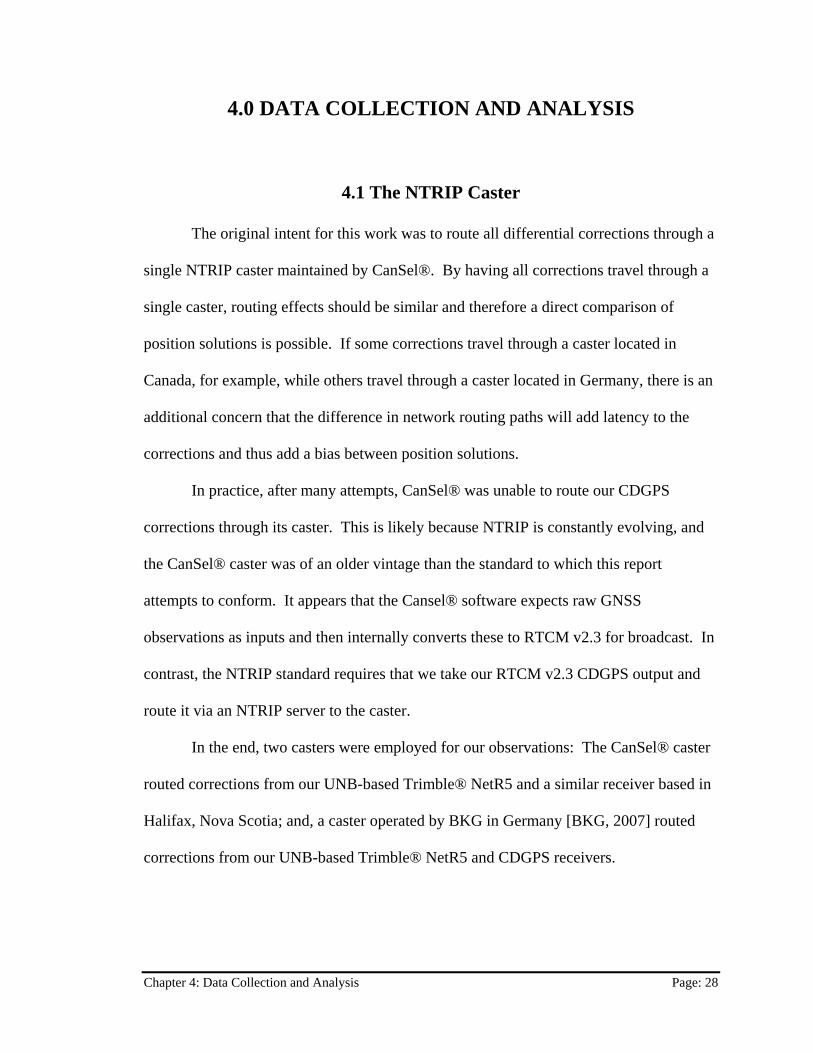
Figure 4.2.1 shows the main screen of the NTRIP server as it is receiving data via

TCP/IP from the UNB Trimble® NetR5 receiver and transmitting to the NTRIP caster

operated by BKG. Figure 4.2.2 shows the input settings to collect data from the receiver

(outlined in red). Figure 4.2.3 shows the output settings to transmit data to the caster

(outlined in red).

Figure 4.2.1 – The main screen of the “GNSS Surfer” NTRIP server software as it transmits local differential corrections in RTCM v2.3 format from a TCP/IP port to an NTRIP caster located in Germany.


*******

Figure 4.2.2 – The “GNSS Surfer” TCP/IP input configuration screen set to retrieve data from a Trimble® NetR5 receiver located at UNB.

Figure 4.2.3 – The “GNSS Surfer” TCP/IP output configuration screen set to send data to an NTRIP caster operated by BKG in Germany.

CDGPS corrections were received via an existing antenna at UNB. These

corrections are broadcast in a modified version of the RTCA format called MRTCA. As

discussed in Chapter 2, RTCA corrections contain vector corrections that apply over a

wide geographic region (in this case, over the entire country of Canada). These

corrections must be converted into pseudorange corrections (PRCs) utilizing the user’s

current location. This was accomplished using a “CDGPS Receiver” (also know as an

“ePing” receiver) as shown in Figure 4.2.4. This unit uses an internal GPS receiver to

determine its own location and outputs RTCM v2.3 via a RS-232C serial

communications port.


Figure 4.2.4 – A CDGPS Receiver which receives modified RTCA corrections and converts them to RTCM v2.3 corrections. [CDGPS, 2003].

The ePing receiver was connected through a RS-232C serial cable to a

Windows® computer running the GNSS Surfer software already mentioned. Figure 4.2.5

shows the COM port settings employed. Figure 4.2.6 shows the settings to transmit

corrections to the BKG NTRIP caster.

*******

Figure 4.2.5 – The “GNSS Surfer” COM input configuration screen set to retrieve data from a CDGPS ePing receiver located at UNB.

Figure 4.2.6 – The “GNSS Surfer” TCP/IP output configuration screen set to send CDGPS corrections to an NTRIP caster located in Germany.


4.2.3 CDGPS Issues Encountered

4.2.3.1 ePing Receivers Are No Longer Manufactured

Two important factors should be mentioned here. Firstly, the ePing receiver as a

stande-alone unit is no longer commercially available. In the past, a CDGPS user needed

to carry an ePing receiver to generate corrections which would then be fed into a GPS

receiver for application. Although cumbersome, this had the advantage of the user being

able to choose from a wide variety of GPS receivers that had no native support for

CDGPS themselves.

CDGPS receivers are now integrated with GPS receivers built by NovAtel®

[NovAtel, 2007]. (At this time, NovAtel® is the only vendor listed as an “integrator” on

the CDGPS website. A limited number of third-party vendors incorporate NovAtel

solutions into their own receivers.) From a positive point of view, this is much less

cumbersome than the traditional ePing unit solution. From a negative point of view, this

severely limits the number of users who will be able to employ CDGPS solutions, since

mainstream vendors such as Trimble® and Magellan® have not chosen to integrate (yet).

NTRIP could move CDGPS into the mainstream since more and more mapping-

grade GNSS units support digital communications. However, it is not clear how one

would obtain CDGPS corrections to disseminate using NTRIP in the absence of an ePing

receiver. Likely such a solution would require the participation of CDGPS as an entity.


4.2.3.2 Intermittent Problems Encountered with the ePing receiver

After the NTRIP server streams were configured, the intention was to let them run

continuously for the duration of the project. However, we found that the ePing receiver

intermittently ceased functioning every two or three days. In its default mode, the

receiver would power off when certain error conditions arose. This required restarting

both the receiver and the GNSS Surfer NTRIP server software. This also resulted in a

“Notice Advisory Broadcaster Users (NABU)” email being sent to all subscribed users of

the stream noting that the stream was unavailable.

The “CDGPS Receiver Configuration Utility” program [CDGPS, 2007] was

downloaded and used to reconfigure the ePing receiver to stay powered on in the event of

a problem. While this did provide more stability in our streams, it did not deal with the

issue that the ePing receiver apparently fails to work at arbitrary times.

It is noted that another ePing receiver working nearby does not appear to have

such frequent problems. It may be that this particular receiver has hardware problems.

4.3 Data Collection Procedures

4.3.1 GNSS Receiver Selection

From the outset, we were interested in comparing differential corrections

disseminated using the NTRIP protocol. To this end, we looked for a receiver with an

integrated NTRIP client. Cansel® was very gracious in its offer to lend us such a unit

and supplied us with a Trimble® GeoXT handheld as shown in Figure 4.3.1. This is a


single-frequency receiver with a Windows® Mobile PC operating system. Although the

unit has an embedded antenna, we chose to use an existing geodetic quality antenna at

UNB because the GeoXT did not work well in –20C weather.

Figure 4.3.1 – The Trimble® GeoXT Series Handheld. [Trimble, 2007a].

4.3.2 Collecting Data with the Trimble® GeoXT

4.3.2.1 Establishing A Bluetooh® “Bond” With a GSM Mobile Phone

Since the GeoXT that we were using did not have either an integrated GSM data

services or a wireless connection we used a Sony Ericsson T616 GSM-enabled mobile

phone with Bluetooth® connectivity (This phone, with service, was graciously provided

by CanSel®). GSM (Global System for Mobile Communications) is a standard for

cellular phone communications on digital networks. It is arguably the most widely used


cellular standard in the world [GSM, 2007] and is supported in New Brunswick by

Rogers® [Rogers, 2007]. Using this technology, a TCP/IP Internet connection could be

established.

The costs for this service vary based on the amount of data transferred. In March

2007, for example, 200MB of data per month costs approximately C$110. Using our

CDGPS data rate of 0.5 kB/s, 200MB is equivalent to approximately 114 hours of

continual use. It is unlikely that even a daily user would exceed this quantity of data.

Bluetooth® [Bluetooth, 2007] is a standard that allows for wireless data and voice

communications over short distances (under 10 metres). Both the Trimble® GeoXT and

the Sony T616 units support this standard. Once the devices are “bonded” or “paired”,

the GeoXT can seamlessly communicate with the mobile phone to establish a TCP/IP

internet connection.

“Bonding” is a procedure carried out only once between any two Bluetooth®

devices. In our case, the GeoXT (“client” device) scans the Bluetooth® radio frequencies

looking for available “hosts” (our GSM phone). Once discovered, a user enters identical

passwords into both devices and a permanent bond is established. Passwords guarantee

that both users intend a bond to be formed [Trimble®, 2004].

To complete connectivity, a “dial-up network” connection is configured on the

GeoXT. This process tells the receiver to use the Bluetooth® connection as a modem,

includes the GSM dialing sequence required by the mobile phone to connect to the

Internet, and includes the username and account password required to log onto the mobile

service.


4.3.2.2 Configuring COM ports for NMEA

Position solutions can be logged on the GeoXT by either storing them on the local

media or by emitting them in the NMEA-0183 format [NMEA, 2007] through a serial

port and logging them remotely. For normal operations, a user would likely choose to

store solutions locally. However, for this work we specifically want information

regarding the latency of differential corrections. Since we were unable to extract this

information from the locally stored solutions, we elected to capture emitted NMEA

strings.

To enable RS-232C serial output, the Windows® Mobile PC operating system

onboard the GeoXT must be used to enable the serial port. Once this is done, the

TerraSync® software installed on the GeoXT must be configured to output NMEA

strings. In our case, we were interested in receiving NMEA “GGA” messages, which

contain time, position, latency and other relevant data.

TerraSync® [Trimble, 2006] is a user program provided by Trimble® which runs

under the Windows® Mobile PC operating system on the GeoXT. It is through this

software that all GPS data collection operations are carried out. Aside from the system

configurations discussed above, all further GeoXT work is carried out inside TerraSync®

4.3.2.3 Configuring the NTRIP client.

When collecting data using differential corrections, we configured the GeoXT

using the TerraSync® software. This software contains an NTRIP client. Selection of

the data stream (mountpoint) is a two step process. First, the client requests a source-


table containing available mountpoints from the NTRIP caster and then the user selects

the mounpoint they wish to use. Before starting configuration, the GeoXT must already

be connected to the Internet as discussed above.

Although we were able to connect to all desired data sources from both the

Cansel® caster and the BKG caster, we did find nuances with the BKG caster. In

particular, one attribute that NTRIP assigns to a mountpoint is the “Station Number”.

The GeoXT client allows a number to be entered, or the selection “Any” to be chosen.

For the Cansel® caster, “Any” always worked. For the BKG caster “Any” worked only

for our CDGPS stream while a value of zero was required for our NetR5 stream. We

could find no obvious reason for this issue.

In general, once configured correctly, the GeoXT was able to connect to a caster

and establish a differential correction stream in approximately one minute.

4.3.2.4 Starting data collection.

Because we were capturing NMEA strings, very little configuration was needed to

collect data. We chose 5 second epochs since we intended to collect data over long

periods. In addition, when differential corrections were to be applied, we configured the

GeoXT so that it would emit no data at all during epochs when corrections were not

available.


4.3.2.5 Capturing NMEA with Hyperterminal®

NMEA strings were captured to a text file using the Microsoft® Hyperterminal®

program integrated with the Windows® operating system.

4.3.2.6 Problems Encountered with the Trimble® GeoXT

Several problems were encountered while collecting data with the GeoXT. The

most serious of these was the inability to collect data for long periods of time while

differential corrections were being applied. A number of different scenarios arose which

resulted in data sets from the order of one-half hour to eleven hours. It was difficult to

determine the cause of the problem, so the states in which the equipment was found are

described:

1. The GeoXT is still in data collection mode, but the dial-up network

connection is lost.

2. The GeoXT is still powered on but it appears that the GPS unit is

disconnected. That is, it appears that TerraSync® can no longer

communicate with the internal GPS unit.

3. The GeoXT is powered off.

Near the end of our observations, the second problem became dominant. It

became increasingly hard to acquire data for more than one half hour.

A second problem was with regard to NMEA output. Although the NMEA

standard specifies that 4,800 baud is to be used, it was found that data overruns occurred

occasionally. As an experiment the baud rate was changed to 38,400. It was found that


at this setting the Windows® Mobile PC operating system crashed. In order to recover, a

system reset was required. Although no data was lost, all settings were lost, including

Bluetooth® bonding, dial-up networking and NTRIP-related data.

Finally, early on it was found that the screen on the unit became faded and

sluggish in temperatures of -10ºC or lower. Since observations were made in the month

of February when temperatures were routinely lower than this, we were not able to use

the unit outside. This meant that we had to use an external antenna. The Trimble®

GeoXT Datasheet [Trimble, 2007a] says that this unit has a lower limit of -10ºC, thus,

users should beware if they intend to use this unit outdoors during the Canadian winter.

4.4 Solution Comparisons

Although GPS solutions are generally carried out in the WGS-84 datum, RTCM

corrections can be used to translate the final solution to a different datum (see Appendix

E of [RTCM, 2001]). In our case, final solutions are in WGS-84 for uncorrected GPS,

NAD83 (CSRS) for CDGPS and the NetR5 located at Halifax, and ITRF2005 (epoch

2007.0) for the NetR5 located at UNB. Section 4.4.1 will show how solutions were

transformed into ITRF2005 (epoch 2007.0). It is noted that the uncorrected GPS

solutions were left in WGS-84 because it is so close to ITRF [Langley, 2007].

GPS solutions were obtained in geodetic coordinates (latitude, longitude, ellipsoid

height). Since most people have a better feeling for position differences in metres rather

than degrees or seconds, all differences were converted to metres. Section 4.4.2

describes the formulae used for these conversions.


4.4.1 Datum Changes

Solutions derived using differential corrections from CDGPS and the Trimble®

NetR5 located in Halifax were in NAD83 (CSRS). These were converted to ITRF2005

(epoch 2007.0) using the TRNOBS 3D coordinate transformation online application

provided by Natural Resources Canada [NRCan, 2007c].

Established ITRF coordinates for the UNBN antenna [Leandro, 2007] were

entered into the application and subsequently transformed into NAD83 (CSRS). The

difference between these geodetic coordinate values was used to shift all observations.

This operation was valid since our observations were static. Figure 4.4.1 shows the

TRNOBS program screen after execution.


Figure 4.4.1: Output of the TRNOBS 3D coordinate transformation program [NRCan, 2007c].

4.4.2 Conversion From Degrees To Metres

Two-dimensional results shown in this report were computed as follows starting

with geodetic (latitude φ , longitude λ ) values [Santos, 2006]:

Step 1: Compute the difference from a known point

knownobserved φφφ −=Δ (4.1)

knownobserved λλλ −=Δ (4.2)


Step 2: Convert degree differences to distances

( )( ) 2

322

2

sin1

1

φe

eaM−

−= (4.3)

φφ 2222

2

sincos baaN+

= (4.4)

( hM +Δ°

= φ )πδφ180

(metres) (4.5)

( ) φλπδλ cos180

hN +Δ°

= (metres) (4.6)

Step 3: Compute the 2DRMS difference

222 δλδφ +=DRMS (metres) (4.7)

4.4.3 2D Position Scatter Plot

Figure 4.4.2 shows the NMEA position solutions collected between February 2,

2007 and February 12, 2007. It should be noted that, due to equipment problems, data

sets were of different lengths. As will be discussed in Section 4.5, both accuracy and

precision are correlated with collection time. Although all of our data sets are of

sufficient length that the uncertainties have converged to their smallest values, one should

be careful when attempting a direct comparison of the uncertainties shown in this graph.

In general, the scatter plot is not surprising. Uncorrected GPS solutions were at

the few metre level while all corrected solutions were of an improved quality. Local

differential corrections provided the best result: a bias of 20 cm and an uncertainty of


30 cm at 95% confidence. (In this report, “accuracy” or “bias” refers to the horizontal

root-mean-square (RMS) distance of a solution from its known point. “Uncertainty” or

“uncertainty at 95% a confidence level” was determined by computing the RMS distance

of an observation from the mean of the entire set and then ordering these from smallest to

largest and choosing the value 95% into the list. These are presented as

uncertainty). ±=Δ accuracy

Figure 4.4.2: 2D position solutions with uncertainties at 95% confidence.

CDGPS generated the next best solution with a bias of 60 cm and an uncertainty

of 50 cm at 95% confidence. However, is clear from the scatter plot that there is a


northwesterly bias present. It is possible that this is due to datum issues. Appendix E of

the RTCM v2.3 specification allows for a datum change in user position to be made

through the addition of pseudorange corrections [RTCM, 2001]. Normally a GPS

receiver carries out its computations in the WGS-84 datum, and thus solutions obtained

are also relative to this datum. If a reference station generating differential corrections

computes PRCs based on its known position in the WGS-84 datum, then resulting

solutions will continue to be in the same datum. However, if the user computes PRCs

based on its known position in a local datum, then the resulting receiver solutions will be

in the local datum. However, Appendix E warns that this datum transformation brings

with it an error that is proportional to the shift between the local datum and WGS-84.

This error will grow linearly as the user moves away from the reference station. With

CDGPS, reference stations are located throughout Canada. It is possible that the bias we

are seeing is an artifact of this datum change.

The only local corrections that were not statistically equivalent to the known

value of the antenna at a 95% confidence level were generated by the Trimble® NetR5

receiver located in Halifax (approximately 430km from where the solutions were

computed). In this case, two major considerations come into play: the validity of local

differential corrections at such a distance, and the effects of a datum shift, since this

unit’s position was specified in NAD83 (CSRS).

In the work carried out by Monteiro et al., it was found that at this distance from a

DGPS reference station (430 km), the 95% uncertainty was approximately 1.5m

[Monteiro et al., 2004, Figure 7a]. In our case, we have an error of 1.0 m ± 0.7 m at 95%

confidence. Even though we have different equipment and observation times, we can see


that our bias is well within the bounds of expectation. To explore this more fully,

intermediate reference stations should be set up, perhaps every 100 km and in various

directions.

Again, with the Halifax NetR5, a datum shift comes into play. Although we did

not oversee the implementation of this receiver ourselves, the vendor states that the

coordinates of this station were computed through both a three-day set of observations

processed with the “CSRS – PPP” program provided by Natural Resources Canada

[NRCan, 2007b] and through baseline observations with nearby Canadian Active Control

Stations [NRCan, 2007a]. Resulting coordinates were entered into the unit in NAD83

(CSRS) and thus, receiver solutions were in this datum also.

Knowing this information, it is interesting to note that before the datum shift from

NAD83 to ITRF (described in §4.4.1) was applied, the solution set statistically agreed

with the known coordinate values. Once the shift was applied, the solution no longer

agreed. This would lead one to question the configuration of the receiver in Halifax.

However, as will be seen in the next section, the height solutions exhibited the opposite

behaviour.


4.4.4 Height Time Series Plot

Figure 4.4.3 shows the height solutions extracted from the NMEA observations.

As with the 2D solutions, we see a clear improvement in quality between different

techniques. Uncorrected GPS was the worst, wide area was significantly improved, and

local differential corrections were the best. Unlike the horizontal case, all solutions were

in statistical agreement with the known height of the antenna at a 95% confidence level.

It is observed that height uncertainties were about 50% greater than the

corresponding horizontal certainties for uncorrected solutions. This follows the general

rule of thumb that horizontal positions are more accurate than heights because

geometrically satellites are always above the user, whereas, horizontally they virtually

surround the user. For corrected solutions, the uncertainties remained constant. This

would imply that differential corrections also account for the geometrical weakness in the

satellite constellation.

With the height solutions, we see the opposite behaviour seen with the 2D

position solutions with the NetR5 receiver located in Halifax. In this case, after

performing the datum shift from NAD83 (CSRS) to ITRF, a bias of only 50 cm

remained. If this shift was not made, the bias increases to 80 cm. Though both solutions

are within the confidence region computed, it seems that applying the shift is better than

not applying it. Thus, whereas the 2D solution indicated that reference receiver

configuration issues might be present, the height solution indicates that the configuration

is correct.

From this data, we also see that although the Halifax corrections result in

solutions centred on the correct value, both the bias and the uncertainty have increased


five-fold from the local corrections generated at UNB. As discussed in Chapter 2, this

decrease in accuracy and precision with increasing receiver separation is exactly the

behaviour expected.

Figure 4.4.3: Ellipsoid height solutions with uncertainties at 95% confidence.


4.5 Precision Versus Observation Time

Up to this point we have examined position and height solutions that resulted

from long observation periods. A more pragmatic question pertains to the amount of

time required to achieve a particular accuracy with and without differential corrections.

To address this question, data sets were submitted to a moving average window

process. In the first iteration, the observation with the largest horizontal RMS error was

found and stored. In the second iteration, each neighbouring set of epochs was averaged

and the worst average epoch was stored. With each successive iteration, the window-size

was increased by one epoch. When window sizes increased past 10 epochs in length (that

is, for the majority of the processing), the RMS values for each window were ordered,

and the 95th-percentile value was stored. Figure 4.5.1 illustrates this process.

1 2 3 4 5 6 7 Iteration 1: a) Compute mean horizontal RMS for

neighbouring epochs b) Keep the worst value

1,2σ

2,2σ

3,2σ

1 2 3 4 5 6 7

1,3σ

2,3σ

3,3σ

Epoch Solution – Known Position

Iteration 2: a) Compute mean horizontal RMS for

neighbouring epochs b) Keep the worst value

> 10 iterations: a) Compute mean horizontal RMS for

neighbouring epochs b) Order values smallest to largest. c) Keep the 95th percentile value

Figure 4.5.1: Moving average-window algorithm used to compare uncertainty with collection time.


4.5.1 Horizontal Positioning

Figure 4.5.2 illustrates the convergence of corrected and uncorrected solutions as

collection time increases. It should be recalled that the data sets were not of uniform

length. This means that the complete set of horizontal error values for uncorrected

solutions came from an 11-hour sample, while data sets for corrected positions came

from samples of only a few hours in length. As will be discussed shortly, this should not

cause much concern because corrected solutions appeared to converge on their best

values at a faster rate than the uncorrected solutions.

Figure 4.5.2: 2D position uncertainties versus observation time at 95% confidence.


The uncorrected solution actually worsens in accuracy over the first 20 minutes of

observation. In fact, it is only after about 40 minutes that the solutions approach the 2-

metre level and begin to slowly but steadily decrease with time. The solutions

augmented with differential corrections generated at UNB show a similar behaviour,

however, they achieve a stable 30 cm-level after only about 10 minutes.

CDGPS and the solutions augmented with corrections generated 430 km away in

Halifax, show a different behaviour. The Halifax-corrected solutions start at a 1.7-metre

level of accuracy and then increase in accuracy approximately linearly over the next two

hours until they reach a 1.3-metre level. Conversely, CDGPS immediately achieves an

80 cm-level accuracy, which it maintains throughout the data collection period with very

little improvement.


4.5.2 Height Positioning

Figure 4.5.3 shows the 95-percentile height uncertainties from the corrected and

uncorrected observations. As can be seen, the situation with heights is dramatically

different than that with horizontal positions.

Figure 4.5.3: Height uncertainties at 95% confidence.

As in the horizontal case, for early periods height accuracy actually worsens for

the uncorrected solutions. However, after approximately 10 minutes, the accuracy


improves in an exponential manner, reaching the 1.5-metre level after two hours of

observation.

Solutions augmented by local corrections generated at UNB do not share this

behaviour. They appear to immediately achieve the 30 cm level and make only slight

improvements over the next two hours.

CDGPS height solutions improve in accuracy by 0.5 metres over a two-hour

observation period. This is in contrast to the horizontal situation, where a steady error

level was maintained throughout the observation period.

Finally, solutions augmented by corrections generated in Halifax start at the

metre-level and actually reach the same 30 cm level of accuracy achieved by the UNB

corrections after two hours of observations.

4.6 Latency Comparisons

Latency is the elapsed time between when a PRC initially becomes valid and the

time when it is actually applied to observations. Range-rate corrections (RRCs), supplied

by the source of differential corrections, may be generated to account for the change in

PRC during the latent period. In our case, RRCs were generated for NetR5 corrections

but not for CDGPS corrections. Latencies are included in the GGA sentence of NMEA

output. These are plotted in Figure 4.6.1. (Note that our receiver was programmed to

cease computing solutions if corrections were unavailable for greater than four minutes.)

As can be seen, latencies were generally under 10 seconds. The CDGPS


corrections had uniformly higher latencies than either of the other solutions. The NetR5

receiver located in Halifax had the lowest latencies, in the order of 3 seconds. Using

packet-watching software owned by CanSel® it was determined that the UNB network

contributed approximately 3 seconds to the latency values.

We see also that the mean of the CDGPS latencies is only 0.4s larger than the

mean of the NetR5 at UNB. However, the CDGPS uncertainty spread is almost double

that of the local NetR5.

Figure 4.6.1: Latency comparison of differential corrections.

Spikes on the latency graph denote points in time where corrections were

disrupted. CDGPS had the worst problem with this issue. Figure 4.6.2 shows the


correlation between latency and position solutions. From this we can see that there were

three occasions during the data collection where corrections ceased for more than 4

minutes, each causing the unit to stop producing position solutions. The reasons for these

disruptions were unclear but were due either to the ePing receiver itself or to the CDGPS

system.

During the data collection we saw 3 periods where the Halifax data was latent by

approximately 10 seconds. The final spike shown in Figure 4.6.1, however, was caused

by a loss of Bluetooth® connection between the GNSS receiver and the mobile phone.

Figure 4.6.2 compares latency with 2D position solutions.

Figure 4.6.2: Correlation of CDGPS 2DRMS with correction latency.


The cross-correlation was computed using the standard formula [Wolf and

Dewitt, 2000, Eq. 15-1]:

( )( )

( ) ( )∑ ∑

∑∑

−−

−−=

i jji

i jji

BBAA

BBAAc

22 (4.8)

Where: A and B Are the two vectors being compared

A and B Are the mean values of these two vectors.

For all data sets, the cross-correlation between latency and accuracy was very

nearly zero, indicating that under normal conditions the position solutions were not

significantly affected by latency. However, as shown in Figure 4.6.3, the solution

accuracy can quickly degrade once corrections stop arriving.

Monteiro et al., note that most GNSS receivers are configured to cease using

PRCs and their associated RRCs after a latency period of 4 minutes [Monteiro et al.,

2004]. They propose that this limit was chosen in an era when Selective Availability was

in place and that in the common era, a 4 minute cap on PRCs is unwarranted. However,

here we see that error doubled during this 4 minute period. It would be interesting to see

how much more the solution would degrade with time. If the observed trend were to

continue as shown in our figure, errors would likely meet the uncorrected GNSS levels at

a latency of approximately 10 minutes.


Figure 4.6.3: Close-up of correlation of CDGPS 2DRMS with correction latency at a correction outage.


5.0 CONCLUSIONS

In this report, an examination of the dissemination of pseudorange corrections

(PRCs) using the NTRIP specification over the Internet has been carried out. Of interest

have been both the comparison of wide area corrections versus local corrections and the

ability of NTRIP to facilitate the transport of corrections into the field for real-time

application.

Although NTRIP is also able to carry real-time kinematic (RTK) corrections, it is

felt that PRCs still maintain a significant relevance in modern work due to their

significantly cheaper cost and ease of application. Many applications, such as

establishing ground control for satellite imagery and positioning for hydrographic surveys

require only sub-metre-level accuracies. These accuracies were realized in this work

using differential corrections and NTRIP.

In the following sections, comments will be made regarding NTRIP, CDGPS and

local DGNSS.

5.1 NTRIP

NTRIP is still in its formative stage. Due to this, we encountered problems such

as the inability to connect our NTRIP server to the CanSel® network, and difficulty in

configuring freeware NTRIP server software to accept corrections from a local serial

port. However, the specification itself seems strong and the fact that the open-ended

design allows dissemination of any type of binary stream, and not simply RTCM, will

ensure its relevance in the future.

Chapter 5: Conclusions Page: 58

In the current market, the biggest obstacle is connectivity. The availability of

GSM in Canada is a relatively recent advent and the cost is still fairly high. The Rogers®

GSM service used for this work is available on the order of $110/month or $1320/year

plus phone equipment. In addition to this cost, the expense of either producing

differential corrections or subscribing to a commercial service must be considered.

This report did not explore the current geographical coverage for mobile phone

connectivity in New Brunswick. However, before one committed to this technology, one

would want to ensure that cell phone coverage was available in the intended regions of

use. To date, one can be confident of coverage in the corridor occupied by the Trans

Canada Highway, while more remote regions may not provide sufficient signal.

The future for NTRIP and other Internet-based services is bright. The last twenty

years has seen a rapid rise of the Internet. The last ten years has seen cell phone

technology gain popularity to the stage where we now see elementary school children

with mobile phones. Today, we are seeing a rapid merging of the two technologies as the

entertainment industry strives to provide music and movies through the mobile network.

In addition, wireless Internet is coming into age. Projects such as the Fredericton eZone

[City of Fredericton, 2007] allow free Internet access from many public places within the

city limits. As time passes, Internet access will become ubiquitous in our environment.

Under these circumstances, NTRIP will flourish.

5.2 CDGPS

Currently CDGPS is of limited use to the general population of Canada because it

is not supported by the mainstream GNSS receiver market. In the past, users have had to


purchase an external ePing receiver, which could receive satellite broadcasts and forward

them in RTCM format to a GNSS receiver. Today, ePing receivers are no longer in

production, and so new users must typically buy a NovAtel®-based GNSS receiver

solution. When one compares this to the FAA’s Wide Area Augmentation System

(WAAS), which is integrated into virtually every receiver solution now on the market,

one sees why the general public has never heard of CDGPS.

NTRIP could be the technology to bring CDGPS to the mass population, since

virtually all GNSS receivers do accept RTCM PRC corrections. Such a solution would

still be cumbersome for receiver units that do not support NTRIP natively. One could

envision two scenarios for implementation. In the first, CDGPS would stream raw wide

area (that is, GPS*C) corrections over the Internet via NTRIP. Clients would need a

mobile PC unit with an NTRIP client embedded and a software program to localize these

corrections to RTCM and forward them to the GNSS receiver. In the second scenario,

CDGPS would set up a full NTRIP caster system. In requesting a mountpoint, NTRIP

clients would transmit their own approximate location. The CDGPS caster would then

localize the corrections and transmit RTCM. The latter scenario might be what is

required to encourage more users to employ the system.

Another issue that should be addressed for CDGPS to become a mainstream

solution is its interaction with the public. The CDGPS website [CDGPS, 2007] appears

to have not been updated in quite some time. It still appears to promote the ePing

receiver, though this avenue has been terminated. In addition, there are apparently

software toolkits available for end-users to support CDGPS, but there is no mention of


them on the website. CDGPS needs to provide an environment where the general public

can interact.

Finally, CDGPS needs to provide more analysis of performance on their website.

Currently, the most recent document is dated in 2003 and provides an indication of initial

performance of the system. The types of questions that most potential end-users will

have are more of the form addressed in this report: what accuracy can be expected, what

observation times are required, and how can various types of equipment can be

configured to accept corrections? Some comment on the datum shift from WGS-84 to

NAD83 (CSRS) should also be made, along with the variation effects across the country.

5.3 Local DGPS

Local DGPS vastly outperformed all other solutions tested in this report. Partly,

this was due to the fact that our corrections were generated at the same location as the

position solutions were obtained. This does not give a true sense of the accuracy of

corrections, as is seen by the Halifax results. The effects of increasing distance on

corrections have been examined by Monteiro et al., but should be examined by any user

intending to make use of local corrections.

NTRIP provides an interesting opportunity in the Canadian and New Brunswick

context. Canada currently operates 46 active control stations [NRCan, 2007a]. New

Brunswick also operates a more densified network of several active control stations [SNB

NRCan, 2007a]. Each of these stations consists of a dual-frequency GNSS receiver and

is connected to the Internet such that users can obtain observation files on an hourly or

daily basis. By simply forwarding the raw observations through a NTRIP caster, users


would be able to generate their own RTK or PRC corrections. Alternatively, RTCM

streams could be generated by the stations and streamed through an NTRIP caster, further

simplifying the user experience. Given that the infrastructure is already in place in both

jurisdictions, a huge gain could be made for very little cost. Extra effort should be made

by a service organization to provide studies to guide end-users regarding accuracy

expectations and observation time requirements.


References

Bluetooth (2007). “Bluetooth® Basics” [On-Line] March 2007 http://www.bluetooth.com/Bluetooth/Learn/Basics/

Bundesamt für Kartographie und Geodäsie (BKG) (2005). “NTRIP: Networked

Transport of RTCM via Internet Protocol” [On-Line] March 2007 http://igs.bkg.bund.de/index_ntrip_down.htm

Bundesamt für Kartographie und Geodäsie (BKG) (2007). “NTRIP Software

Downloads” [On-Line] March 2007 http://igs.bkg.bund.de/index_ntrip_down.htm

CDGPS (2003). “CDGPS Receiver: User’s Guide, Version 1.0 August 15, 2003”

Base Mapping and Geomatic Services, Ministry of Sustainable Resource Management, Province of British Columbia, Canada. [On-line] March, 2007. http://www.cdgps.com/e/cdgps_documents/cdgpsradiousersmanualv1.pdf

CDGPS (2007). http://www.cdgps.com Chen, Ruizhi and Xiyin Li (2004). “Virtual Differential GPS based on SBAS signal”,

GPS Solutions, Vol. 8, pp.238-244. City of Fredericton (2007). “Fred-eZone: Free WiFi for Fredericton”

[On-Line] March 2007 http://www.fred-ezone.ca

Dare, P. (2005) “GGE 2012 Class Notes, Fall, 2005”

Department of Geodesy and Geomatics, University of New Brunswick, Canada. Garmin (2007). Garmin® eTrex Legend

[On-Line] March 2007 http://www.garmin.com/products/etrexLegend/

GSM (2007). “Global System for Mobile Communications”

[On-Line] March 2007 http://en.wikipedia.org/wiki/Global_System_for_Mobile_Communications

Leandro, Rodrigo (2007). Personal communications: Coordinates for the UNBN

Antenna. Department of Geodesy and Geomatics, University of New Brunswick, Canada.

References Page: 63

http://www.bluetooth.com/Bluetooth/Learn/Basics/

http://igs.bkg.bund.de/index_ntrip_down.htm

http://www.cdgps.com/e/cdgps_documents/cdgpsradiousersmanualv1.pdf

http://www.cdgps.com/

http://www.fred-ezone.ca/

Misra, P., and P. Enge (2001). Global Positioning System: Signals, Measurements, and

Performance. Ganga-Jamuna Press, Massachusetts, U.S.A.Monteiro, L.S., T. Moore, C. Hill (2005). “What is the accuracy of DGPS?” The Journal of Navigation, Vol 58, pp. 207-225.

Monteiro, L.S., T. Moore, C. Hill (2005). “What is the accuracy of DGPS?”

The Journal of Navigation, Vol 58, pp. 207-225. National Marine Electronics Association (2007). NMEA 0183 Standard

National Marine Electronics Association, Maryland, U.S.A. [On-Line] March 2007 http://www.nmea.org/pub/0183/

Natural Resources Canada (2007a). “CSRS Active Networks Summary”

[On-Line] March 2007 http://www.geod.nrcan.gc.ca/network_a/active_e.php

Natural Resources Canada (2007b). “CSRS-PPP Online Application”

[On-Line] March 2007 http://www.geod.nrcan.gc.ca/ppp_e.php

Natural Resources Canada (2007c). “TRNOBS 3-D Coordinate Transformation Program”

[On-Line] March 2007 http://www.geod.nrcan.gc.ca/apps/trnobs/index_e.php

NovAtel (2007). http://www.novatel.ca/ Rogers (2007). Rogers GSM/GPRS Products

[On-Line] March 2007 http://www.shoprogers.com

RTCA (1996). Minimum Operational Performance Standards For Global Positioning

System / Wide Area Augmentation System Airborne Equipment. RTCA, Inc. Washington, D.C., U.S.A.

RTCA (2007). RTCA Main Web Page

[On-Line] March 2007 http://rtca.org

Radio Technical Commission For Maritime Services (2001). “RTCM Recommended

Standards For Differential GNSS Service, Version 2.3” Radio Technical Commission For Maritime Services, Virginia, U.S.A.

References Page: 64

http://www.nmea.org/pub/0183/

http://www.geod.nrcan.gc.ca/network_a/active_e.php

http://www.geod.nrcan.gc.ca/ppp_e.php

http://www.geod.nrcan.gc.ca/apps/trnobs/index_e.php

http://www.novatel.ca/

http://www.shoprogers.com/

http://rtca.org/

Radio Technical Commission For Maritime Services (2004). “RTCM Standard 10410.0 For Networked Transport of RTCM via Internet Protocol (NTRIP)” Radio Technical Commission For Maritime Services, Virginia, U.S.A.

Santos, Marcelo C. (2006). “GGE 4042 Kinematic Positioning Laboratory Manual, September 2006”. Department of Geodesy and Geomatics, University of New Brunswick, Canada.

Service New Brunswick (2007). “The New Brunswick Active Control Network

(NBACN)” [On-Line] March 2007 https://www.web11.snb.ca/snb7001/e/2000/2922e.asp

Trimble (2004). “GeoExplorer® Series: Getting Started Guide, Version 3.00, February

2004” [On-Line] March 2007 http://www.trimble.com/geoxt_ts.asp?Nav=Collection-10645

Trimble (2006). “TerraSync software: Getting Started Guide, Version 2.60, Revision A,

August 2006” [On-Line] March 2007 http://www.trimble.com/geoxt_ts.asp?Nav=Collection-10645

Trimble (2007a). “GeoXT Handheld Datasheet”

[On-Line] March 2007. http://trl.trimble.com/docushare/dsweb/Get/Document- 262825/13305J_GeoXT_DS_1106_lr.pdf

Trimble (2007b). “Trimble NetR5 Reference Station”

[On-Line] March 2007 http://www.trimble.com/netr5_ds.asp

Trimble (2007c). “Trimble Virtual Reference Station”

[On-Line] March 2007 http://www.trimble.com/vrs.shtml

United States Naval Observatory (2007). NAVSTAR GPS Operation

United States Naval Observatory, Washington, D.C. USA. [Online]: January 2007. http://tycho.usno.navy.mil/gpsinfo.html#st

Weber, G. (2005). “Networked Transport of RTCM via Internet Protocol (Ntrip) – IP-Streaming for Real-Time GNSS Applications”. Presented at the ION GNSS 2005, the 18th International Technical Meeting of the Satellite Division, September 13-16, 2005, Long Beach, C.A., U.S.A.

References Page: 65

https://www.web11.snb.ca/snb7001/e/2000/2922e.asp

http://www.trimble.com/geoxt_ts.asp?Nav=Collection-10645

http://www.trimble.com/geoxt_ts.asp?Nav=Collection-10645

http://trl.trimble.com/docushare/dsweb/Get/Document-%20262825/13305J_GeoXT_DS_1106_lr.pdf

http://trl.trimble.com/docushare/dsweb/Get/Document-%20262825/13305J_GeoXT_DS_1106_lr.pdf

http://www.trimble.com/netr5_ds.asp

http://www.trimble.com/vrs.shtml

http://tycho.usno.navy.mil/gpsinfo.html#st

Wells, D. et. al (1986). Guide To GPS Positioning. Department of Geodesy and Geomatics Engineering Lecture Note No. 58, University of New Brunswick, Fredericton, New Brunswick, Canada, 291pp.

Wolf, Paul R. and B.A. Dewitt (2000). “Elements of Photogrammetry with Applications

in GIS, 3rd Ed.”. McGraw Hill, Toronto, Canada.

References Page: 66

Selected Bibliography

Bates, Regis J. (2002). GPRS: General Packet Radio Service, McGraw-Hill, U.S.A. Chen, Ruizhi and Xiyin Li (?). “Test Results of and Internet RTK System Based on the

NTRIP Protocol”, From BKG website – I am looking for a proper reference as I believe this has been submitted for publication. Finnish Geodetic Institute, Masala, Finland.

Gontran, H., J. Skaloud, P.Y. Gillieron (?). “Photobus: Towards Real-Time Mobile

Mapping”. Geodetic Engineering Laboratory, Lausanne, Switzerland.

Horvath, Tamas (2002). “Performance Comparison of Wide Area Differential GPS

Systems”, Technical Report No. 212. Department of Geodesy and Geomatics, University of New Brunswick, Canada.

Lenz, Elmar (2004). “Networked Transport of RTCM via Internet Protocol (NTRIP) –

Application and Benefit in Modern Surveying Systems”. Presented at FIG Working Week 2004, Athens, Greece, May 22-27, 2004.

Macleod, K. and P. Heroux (2006). “GPS-C Distribution Using NTRIP”. Slides from

paper presented at the NTRIP Symposium and Workshop, Frankfurt, Germany, February 6 & 7, 2006. Author is from Geodetic Survey Division, Natural Resources Canada.

Milner, James (2004). “The development and enhancement of GNSS/GPS infrastructure

to support Location Based Service Positioning Systems in Victoria”. Presented at the 2004 International Symposium on GNSS/GPSS, December 6-8, 2004, Sydney, Australia.

Pala, A., G. Sanna, G. Vacca (?). “Real Time Mapping with DGPS-Enabled Navigation

Equipment”. Department of Structural Engineering, University of Cagliari, Cagliari, Italy.

Peterzon, Martin (2004). “Distribution of GPS Data via Internet”. Geodetic Research

Department, National Land Survey of Sweden. RTCM (2004). “RTCM Recommended Standards For Differential GNSS Service,

Version 3.0” Radio Technical Commission For Maritime Services, Virginia.

Rus, Tiberiu, Johan Neuner (?). “D-GNSS Accuracy Tests At BUCU EPN Station”.

Faculty of Geodesy, Technical University of Civil Engineering, Bucharest, Romania.

Selected Bibliography Page: 67

Stöcker, Dirk (). “Improving L1/CA-GPS receiver performance with a wide area GPS

network and internet technology”, EuroNav Service, GmbH. Waltersdorf, Germany. (Referenced on BKG website.)

Weber, G., H. Gebhard, D. Dettmering (2003). “Networked Transport of RTCM via Interent Protocol (Ntrip).” Presented at the IAG meeting, Saporro, Japan, June 30 – July 11, 2003.

Yan, T.S. (2004). “Benefits of Telecommunications Technology to GPS Users”.

Presented at the 2004 International Symposium on GNSS/GPSS, December 6-8, 2004, Sydney, Australia.

Selected Bibliography Page: 68

a comparison of local and wide area differential corrections disseminated using ... · corrections...

Documents