Cornell University School of Hotel AdministrationThe Scholarly Commons

Articles and Chapters School of Hotel Administration Collection

9-2003

A Comparison of Forecasting Methods for HotelRevenue ManagementLarry R. WeatherfordUniversity of Wyoming

Sheryl E. KimesCornell University School of Hotel Administration, sek6@cornell.edu

Follow this and additional works at: http://scholarship.sha.cornell.edu/articles

Part of the Hospitality Administration and Management Commons

This Article or Chapter is brought to you for free and open access by the School of Hotel Administration Collection at The Scholarly Commons. It hasbeen accepted for inclusion in Articles and Chapters by an authorized administrator of The Scholarly Commons. For more information, please contacthlmdigital@cornell.edu.

Recommended CitationWeatherford, L. R., & Kimes, S. E. (2003). A comparison of forecasting methods for hotel revenue management [Electronic version].Retrieved [insert date], from Cornell University, School of Hotel Administration site: http://scholarship.sha.cornell.edu/articles/753

A Comparison of Forecasting Methods for Hotel Revenue Management

AbstractThe arrivals forecast is one of the key inputs for a successful hotel revenue management system, but noresearch on the best forecasting method has been conducted. In this research, we used data from ChoiceHotels and Marriott Hotels to test a variety of forecasting methods and to determine the most accuratemethod. Preliminary results using the Choice Hotel data show that pickup methods and regression producedthe lowest error, while the booking curve and combination forecasts produced fairly inaccurate results. Themore in-depth study using the Marriott Hotel data showed that exponential smoothing, pickup, and movingaverage models were the most robust.

Keywordsforecasting competitions, forecasting practice, comparative methods, time series, univariate: exponentialsmoothing, holt-winters, regression

DisciplinesHospitality Administration and Management

CommentsRequired Publisher Statement© Elsevier. Final version published as: Weatherford, L. R., & Kimes, S. E. (2003). A comparison of forecastingmethods for hotel revenue management. International Journal of Forecasting , 19(3), 401-415. doi:10.1016/S0169-2070(02)00011-0.

This version of the work is released under at Creative Commons Attribution-NonCommercial-NoDerivatives4.0 International License. Reprinted with permission. All rights reserved.

This article or chapter is available at The Scholarly Commons: http://scholarship.sha.cornell.edu/articles/753

A comparison of forecasting methods for hotel revenue management

Larry R. Weatherford Corresponding Author University of Wyoming

Sheryl E. Kimes

Cornell University

Abstract

The arrivals forecast is one of the key inputs for a successful hotel revenue management system, but no research on the

best forecasting method has been conducted. In this research, we used data from Choice Hotels and Marriott Hotels to

test a variety of forecasting methods and to determine the most accurate method. Preliminary results using the Choice

Hotel data show that pickup methods and regression produced the lowest error, while the booking curve and combination

forecasts produced fairly inaccurate results. The more in-depth study using the Marriott Hotel data showed that

exponential smoothing, pickup, and moving average models were the most robust.

Keywords: Forecasting Competitions; Forecasting practice; Comparative methods, time series; Time series, univariate:

exponential smoothing; Holt-Winters, regression

1. Introduction

Yield, or revenue, management, as commonly practiced in the hotel industry helps hotels decide on the most profitable

mix of transient business. The transient forecast is the key driver of any revenue management system, yet no published

research addresses the accuracy of hotel forecasting methods for transients. Kimes (1999) has previously studied the issue

of hotel group forecasting accuracy.

Accurate forecasts are crucial to good revenue management. Lee (1990) found that a 10% increase in forecast accuracy

in the airline industry increased revenue by 0.5-3.0% on high demand flights. A recent Wall Street Journal article said that

Continental Airlines increased profits by $50 to $100 million per year from the use of their revenue management system

(McCartney, 2000). Detailed forecasts are the major input to most revenue management systems, and without accurate

forecasts, the rate and availability recommendations produced by the revenue management system may be highly

inaccurate.

The data that is used for hotel forecasting has two dimensions to it: when the reservation was booked and when the

room was consumed. The booking information gives the manager additional detail which can be used to update the

forecast. Without this information, the manager would have to rely solely on the historical information on the daily

number of arrivals or rooms sold.

In this research, we tested a variety of different forecasting methods on data from four hotels operated by Choice

Hotels and two hotels operated by Marriott Hotels. The accuracy of the various methods was determined and methods

providing the most accurate and stable forecast were identified. By having this information, hotels can more effectively

and profitably use their revenue management systems. In addition, improved forecast accuracy can lead to better staffing,

purchasing and budgeting decisions.

We will begin with a description of the forecasting methods available, followed by a discussion of the other important

issues associated with forecasting for revenue management. In addition to the method selection, other important

questions which must be addressed include the type of forecast (arrivals or room nights), the level of aggregation (total,

by rate category, by length of stay, or some combination), the type of data (constrained or unconstrained), the amount of

data, the treatment of outliers, and the measurement of accuracy.

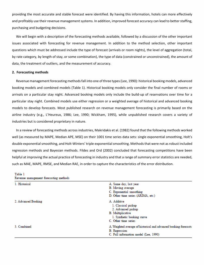
2. Forecasting methods

Revenue management forecasting methods fall into one of three types (Lee, 1990): historical booking models, advanced

booking models and combined models (Table 1). Historical booking models only consider the final number of rooms or

arrivals on a particular stay night. Advanced booking models only include the build-up of reservations over time for a

particular stay night. Combined models use either regression or a weighted average of historical and advanced booking

models to develop forecasts. Most published research on revenue management forecasting is primarily based on the

airline industry (e.g., L’Heureux, 1986; Lee, 1990; Wickham, 1995), while unpublished research covers a variety of

industries but is considered proprietary in nature.

In a review of forecasting methods across industries, Makridakis et al. (1982) found that the following methods worked

well (as measured by MAPE, Median APE, MSE) on their 1001 time series data sets: single exponential smoothing, Holt’s

double exponential smoothing, and Holt-Winters’ triple exponential smoothing. Methods that were not as robust included

regression methods and Bayesian methods. Fildes and Ord (2002) concluded that forecasting competitions have been

helpful at improving the actual practice of forecasting in industry and that a range of summary error statistics are needed,

such as MAE, MAPE, RMSE, and Median RAE, in order to capture the characteristics of the error distribution.

2.1. Historical models

Traditional forecasting methods such as exponential smoothing in its various forms, moving average methods (simple

and weighted), as well as linear regression can be used to derive forecasts based solely on historical arrivals. Early research

relied on fairly simple approaches, while later research advocated ARIMA time series methods. In the ‘classic’ Makridakis

forecasting competition (Makridakis et al., 1982), it was found that complex or statistically sophisticated methods (like

ARIMA) did not, in general, outperform simple ones.

Typical of the simple methods used in industry, Littlewood (1972) proposed that a mean of historical bookings on

previous departures of the same flight be used to estimate the number of bookings on future flights. In 1974, Duncanson,

in his study of forecasting at Scandinavian Airlines System (SAS), incorporated seasonal analysis and exponential

smoothing into his forecasting methods and also studied the use of historical time series analysis. His research

concentrated on stable European markets and did not disaggregate the demand by rate category or consider

unconstrained demand.

Sa (1987) studied ARIMA methods for a single fare class on a single flight number. The results were not promising, and

he switched his study to the use of multiple regression. Lee (1990) also suggested using an ARIMA method to develop a

historical booking forecast.

Unpublished hotel industry research shows two methods being used to estimate historical demand. Some companies

use the number of rooms or arrivals for the same day of the previous year to estimate the historical forecast, while other

companies use the Holt-Winters exponential smoothing method to estimate the long-term forecast.

2.2. Advanced booking models

Advanced booking models can be divided into additive models and multiplicative models. Additive models assume that

the number of reservations on hand at a particular day before arrival (or reading day) is independent of the final number

of rooms sold, while multiplicative models assume that the number of reservations yet to come is dependent on the

current number of reservations on hand.

2.2.1. Additive models

Adams and Vodicka (1987), in their study of forecasting at Qantas Airlines, developed short-term forecasts for just 1

week before departure. They used fairly simple methods which relied on subjective marketing estimates and simple

averages of segment class reservations.

L’Heureux (1986) discussed the classical ‘pickup’ (pickup is defined as the number of reservations picked up from a

given point in time to a different point in time over the booking process) method and the advanced pickup method in an

airline context. The classical pickup method determines the average (or weighted average) of reservations picked up

between different reading days (e.g., between 120 days out and 90 days out) for departed flights (e.g., CP 121 Calgary-

Montreal) for a particular day of week to forecast the future pickup between the same reading days for the same flight

number on the same day of week in the future. The advanced pickup method is similar to the classical pickup method,

with the extension that it includes relevant data from all flights, even those that have not yet departed.

2.2.2. Multiplicative and time-series methods

Lee (1990) suggested two types of advanced booking methods: (1) the synthetic booking curve model and (2) a time

series of advanced booking models. The synthetic booking curve model attempts to describe the shape of the booking

curve (e.g., piecewise linear or nonlinear), while the time series method expresses the total bookings at time t before

departure as a time series of total bookings at earlier points.

2.3. Combined forecast methods

Combined forecasting methods can use regression methods, or a weighted average of a historical forecast and an

advanced booking forecast, or a full information model. Fildes and Ord (2002) concluded from the research literature that

combination forecasts generally yielded greater forecast accuracy. Ben-Akiva (1987) developed fare-class-specific and

flight-specific forecasts using a time series method for historical bookings, a regression method for advanced bookings,

and a combined model with both advanced bookings and historical data. He found that the combined approach worked

better, but he did not consider unconstrained demand (i.e., demand unconstrained by the capacity of the plane or hotel).

In addition, his forecasts were made on monthly data, and therefore do not provide the necessary level of detail.

Sa (1987) used multiple regression to develop a combined forecast. The dependent variable used was reservations

remaining while the independent variables included the number of reservations on hand, a seasonal index, a weekly index,

and an average of historical reservations remaining. The regression method was run for various days before departure (t

= 7, 14, 21, and 28). Unfortunately Sa did not test the accuracy of his methods and did not consider the impact of

unconstrained demand.

Lee (1990) modeled the airline booking process as a stochastic process with interspersed reservations and cancellations.

He tested two combined methods including: (1) a weighted average of the advanced bookings and historical bookings

models, and (2) a full information model that views the booking process as a time series of historical bookings. The full

information combined (FIC) model found maximum likelihood estimates for parameters that combined information on

bookings on hand, previous flights’ bookings-to-come, previous flights’ final bookings and a ratio of seats sold in discount

buckets into a single model. He found that the FIC method outperformed the ‘standard’ eight period moving average

method (i.e., it reduced the mean absolute error by 31% from 6.91 to 4.74).

Wickham (1995) presented a simple linear regression method in which the independent variable was the number of

reservations on hand for a flight at a particular reading day and the dependent variable was the final number of seats sold.

Skwarek (1996), Weatherford (1997) and Zickus (1998) have presented a similar approach.

Unpublished, proprietary hotel industry methods advocate a weighted average of the historical forecast and the

advanced booking forecast. When the day of arrival is far in the future, more weight is put on the historical forecast,

whereas when the day of arrival is imminent, more weight is put on the advanced booking forecast.

2.4. Method comparison

Wickham (1995) studied the accuracy of a variety of forecasting methods for a set of airline data. He studied both (a)

historical forecasting methods (simple averages and weighted averages) and (b) pickup- based forecasting methods

(classical and advanced pickup methods) and found that in general, pickup- based forecasting methods provided the most

accurate forecasts of the two groups he studied.

Weatherford (1998) compared additive methods, multiplicative methods, and regression in an airline context and

found that additive methods and regression out-performed multiplicative methods.

Zickus (1998) found that the choice of unconstraining method, combined with the choice of forecasting method and

optimization method impacted revenue produced.

2.5. Forecasting methods used in this paper

In this research, we tested seven different forecasting methods:

1. Simple exponential smoothing, using a values between 0.05 and 0.95.

2. Moving average methods with the number of periods in the average varying between 2 and 8.

3. Linear regression methods which assumed that there was a correlation between the number of reservations on

hand currently (day n) and final number of reservations (day 0) (e.g., Forecast@Day 0 = a + b X Bookings@Day n).

4. Logarithmic linear regression methods (e.g., log(Forecast@Day 0) = a + b X log(Bookings at Day n).

5. Additive, or ‘pickup’, method which adds the current bookings to the average historical pickup in bookings from the

current reading day to the actual stay night (e.g., Forecast@Day 0 = Bookings@Day n + Average Pickup(Day n to Day

0).

6. Multiplicative method, which multiplies the current bookings by the average historical pickup ratio in bookings from

the current reading day to the actual stay night. (e.g., Forecast@Day 0 = Bookings@Day n X Average Pickup Ratio(Day

n to Day 0).

7. Holt’s Double Exponential smoothing, using a values between 0.05 and 0.95, ß values between 0.05 and 0.95.

3. Other forecasting issues

As mentioned earlier, the choice of forecasting method is not the only issue which must be addressed. Managers must

also consider what to forecast (arrivals or room nights), the level of aggregation (total, by rate category (RC), by length of

stay (LOS), or some combination), the type of data (constrained or unconstrained), the number of periods to include in

the forecast, which data to use, outliers and the measurement of accuracy (see Table 2). Because airline and hotel data

contain atypical events (e.g., promotions, conventions, weather, holiday weekends, crashes, wars), outliers must be

removed.

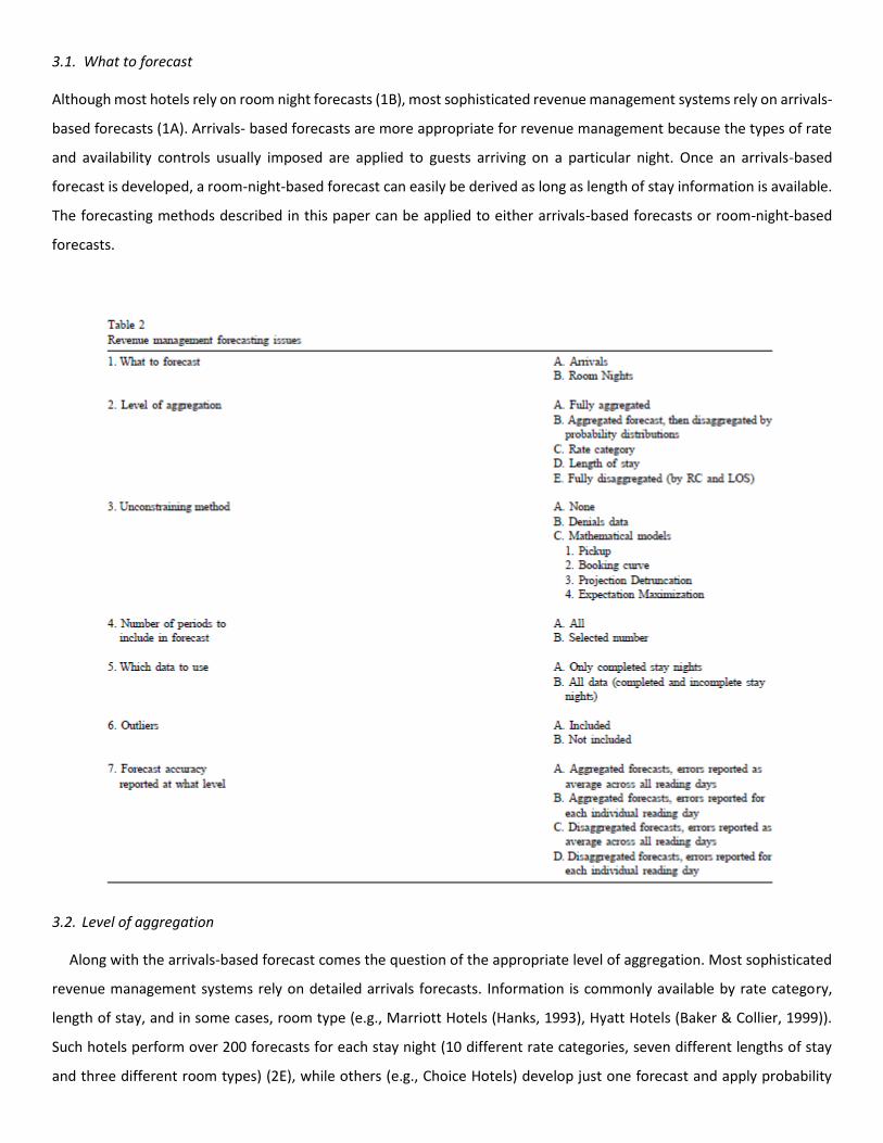
3.1. What to forecast

Although most hotels rely on room night forecasts (1B), most sophisticated revenue management systems rely on arrivals-

based forecasts (1A). Arrivals- based forecasts are more appropriate for revenue management because the types of rate

and availability controls usually imposed are applied to guests arriving on a particular night. Once an arrivals-based

forecast is developed, a room-night-based forecast can easily be derived as long as length of stay information is available.

The forecasting methods described in this paper can be applied to either arrivals-based forecasts or room-night-based

forecasts.

3.2. Level of aggregation

Along with the arrivals-based forecast comes the question of the appropriate level of aggregation. Most sophisticated

revenue management systems rely on detailed arrivals forecasts. Information is commonly available by rate category,

length of stay, and in some cases, room type (e.g., Marriott Hotels (Hanks, 1993), Hyatt Hotels (Baker & Collier, 1999)).

Such hotels perform over 200 forecasts for each stay night (10 different rate categories, seven different lengths of stay

and three different room types) (2E), while others (e.g., Choice Hotels) develop just one forecast and apply probability

distributions of rate category and length of stay (2B). Research on forecast disaggregation for hotels has shown that

detailed disaggregate forecasts outperform more general aggregate forecasts that are then broken down to the

disaggregated level by any reasonable scheme (Weatherford et al., 2001). The airlines face a similar problem with origin-

destination forecasting and observed errors have been high when forecasts are highly disaggregated (Weatherford, 1998).

3.3. Unconstraining method

Another important issue for revenue management forecasts is the need to provide both constrained (3A) and

unconstrained (3B and 3C) forecasts. Historical room sales are constrained by the capacity of the hotel and by the booking

limits placed on various rate categories and lengths of stay. Some method of determining the true, unconstrained demand

is necessary for most revenue management optimization methods. Lee (1990) and Wickham (1995) tested the impact of

truncated and censored data on the accuracy of the forecast and found that forecasts made with unconstrained data were

more accurate.

Demand can be unconstrained by using either reservation denial data (3B in Table 2) (Orkin, 1998) or by using

mathematical models (3C in Table 2). According to the authors’ industry knowledge, denial data maintained by most hotels

and airlines is considered to be unreliable, so most revenue management consulting firms have turned to mathematical

models. The appropriate mathematical model to use depends on the underlying probability distribution of reservation

data. Belobaba (1985), in his study of TWA reservations data, found that demand was approximately normally distributed.

Other published research (Smith and Penn, 1988; Lee, 1990) has suggested either a Poisson, lognormal or g distribution.

Normal distributions present practical difficulties because of the truncation at zero (there cannot be negative reservations)

and capacity or booking limit constraints. In addition, the normal, lognormal and g distributions are continuous

distributions, while reservations data are inherently discrete. If truncation or censoring does occur, a maximum likelihood

estimation should be used to determine the parameters. Maddala (1983) and Schneider (1986) discussed estimating

censored and truncated models with normally distributed data.

A variety of methods have been suggested for unconstraining demand including pickup detruncation (3C1) (Skwarek,

1996), booking curve detruncation (3C2) (Wickham, 1995) and projection detruncation (3C3) (Hopperstad, 1995). Pickup

detruncation and booking curve detruncation are similar in that both look at the number (in the case of pickup) or

percentage (in the case of booking curve) of reservations which were turned away for constrained days. Projection

detruncation assumes a normal distribution and then attempts to iteratively determine the true mean and standard

deviation (Hopperstad, 1995). Weatherford and Polt (2001) investigated three naive methods commonly used by airlines,

as well as booking curve detruncation and projection detruncation (PD) mentioned earlier, and a new statistical method

known as Expectation Maximization (3C4) (abbreviated as EM). They found that both EM and PD performed significantly

better than all other methods as measured by the fact that their estimate of the unconstrained mean was 20-80% larger

than the other methods and much closer to the true mean value.

3.4. Number of periods to include in forecast

Hotels usually face a high degree of seasonality. If only a smaller number of periods (4B) are used (e.g., only the most

recent 8-12 weekly observations) to determine the optimal parameters and generate the forecast, seasonality may not be

adequately addressed. If all available periods (4A) are used (possibly several years worth of observations), seasonality may

be better handled, but the most appropriate number of periods still must be determined. This is a very rich topic that has

not yet been adequately addressed by researchers. It basically involves the tradeoff between including too little data

(missing possible seasonal influences and creating an unstable forecast) versus too much data (creating an unresponsive

forecast that is not dynamic enough).

3.5. Which data to use

Hotels have booking data for not only completed stay nights but also for stay nights which have not yet occurred. The

classical pickup method (L’Heureux, 1986) uses booking data for only completed stay nights (5A) while the advanced

pickup method (L’Heureux, 1986) uses all booking data, even from incomplete stay nights (5B). As an example of an

incomplete stay night, consider a stay night that will occur 2 weeks in the future, for which we do not yet have complete

data (i.e., we have not yet observed the last 2 weeks of the booking process), but for which we have observed the bookings

from 120 days out down to 14 days (2 weeks) out. A similar logic could be applied to other forecasting methods.

3.6. Outliers

When developing forecasts, hotels must decide how to treat holidays, special events and unusual days. In fact, this is

generally true for forecasting in any industry. If outliers are included when developing forecasts (6A), the resulting

forecasts may have increased error. Conversely, if regular stay nights are used to develop the forecasts for holidays and

special events, the forecasts may be extremely inaccurate. Some method of outlier detection and adjustment should be

employed to correct for this problem (6B). An outlier is typically defined as any observation that exceeds the mean± 3

standard deviations. For example, suppose we have 100 observations of demand for a Tuesday night for a particular hotel

with a mean value of 400 and a standard deviation of 20. Based on the above definition of an outlier, we would remove

any observations from our sample of 100 that either exceeded 460 or were smaller than 340.

3.7. Reporting forecast accuracy

When measuring forecast accuracy, the impact on the hotel’s decision making and financial results must be considered.

The level of aggregation of the forecast error is also crucial. Most sophisticated revenue management systems rely on

accurate forecasts of demand by length of stay and rate category. This reliance leads to an emphasis on the accuracy of

very detailed demand forecasts. Unfortunately, the small numbers associated with some of the detailed forecasts (e.g.,

the actual demand for a 6-night length of stay in rate category 4 on a given Thursday night might well be 0) may lead to

higher errors, and if the error is measured as a percentage (as in the case of the Mean Absolute Percentage Error), the

error may appear unusually high (7C in Table 2). For example, if the forecast for a given RC/LOS combination was 0.2 and

the actual value was 0, then the MAPE would be infinite. Therefore, it may be that the MAE is the error measure which is

most meaningful and relevant to the financial losses incurred from inaccurate forecasts. If only overall error is calculated

(7A in Table 2), it would mean that all arrivals for a given night were lumped together (all rate categories and lengths of

stay) and that only the forecast error for this aggregate number was reported. Therefore, the impact on the detailed rate

and availability controls created by the revenue management system, that attempts to manage accept/reject decisions at

the rate category/length of stay level, will be ignored.

Hotels using revenue management typically update forecasts on a daily basis for occupancy dates in the near future (1-

2 weeks) and update on a weekly basis for dates farther away (2-8 weeks). Obviously, errors will vary depending on when

the forecasts are made. When calculating forecast error, hotels can either calculate forecast error for only a particular

forecast update (reading day) (7B and 7D) or average over all reading days (7A and 7C).

3.8. Revenue impact of forecast accuracy

Lee (1990) studied the impact of forecast accuracy on revenue generated for a major US airline. He varied the mean

and standard deviation of the forecast error for four different demand scenarios (low, medium, high and very high),

effectively studying the impact of bias or error in forecasts of airline passengers. Variations in the standard deviation had

little impact on ‘expected’ revenues, but variations in the mean produced substantial changes in expected revenues in

high and very high demand situations. Over-forecasting errors (forecast> actual) caused a larger decline in revenue than

under-forecasting errors. When demand in the higher fare classes was over-forecast, lower fares were then overly

restricted, resulting in a slightly higher yield (equivalent to average daily rate in hotel industry), but a greatly reduced load

factor and a statistically significant decrease in revenue. When demand in the higher fare classes was under-forecast,

higher fares were not sufficiently restricted, resulting in a decrease in yield, an increase in load factor and only a slight,

yet statistically significant decrease in revenue. On high and very high demand flights, he found that a 10% improvement

in forecast accuracy increased revenue by 0.5-3.0%. Because this increase in revenue could be generated by either a higher

yield per passenger (no incremental cost) or higher load factor (a very small incremental variable cost), which is equivalent

to higher average daily rate and higher occupancy rate in the hotel industry, the increased revenue leads to an even higher

percentage increase in profits. Although no airline has as many high/very high demand flights as they would like, all airlines

have some flights that fall into these categories.

Weatherford (1997) reported results using data from Continental Airlines and confirmed that there is a significant

impact on revenue as a result of both under- and over-forecasting. However, he found that the impact of under-

forecasting is worse in cases of high demand/capacity ratios (> = 1.2), with the opposite effect at lower demand/capacity

ratios, albeit a smaller magnitude. He also found the exact opposite effect at Lufthansa Airlines. So, clearly, the result as

to whether over- or under-forecasting is worse depends on the carrier.

4. Methodology

The research was divided into two stages. In the first stage, advanced booking models and combination forecasting

methods were used to develop forecasts for four hotels operated by Choice Hotels. In the second stage, historical booking

models, advanced booking models and combination forecasts methods were used to develop forecasts for two hotels

operated by Marriott Hotels. The purpose of the first stage was to make a preliminary study with the smaller data set of

the first hotel and then in stage two to refine those results with a more complete, in-depth study with the larger amount

of data available for the second hotel.

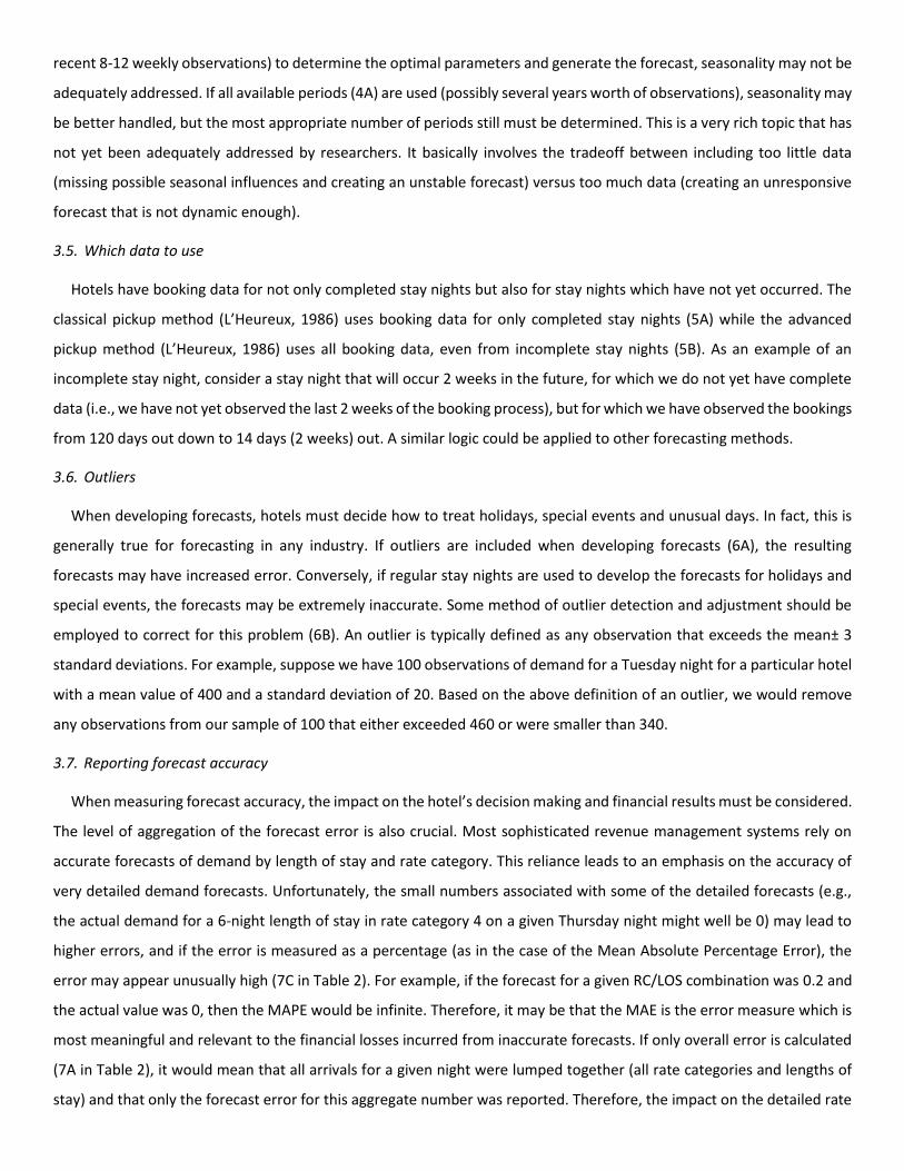
4.1. Stage 1: Choice hotels1

The Choice hotels studied were primarily small roadside hotels (under 150 rooms) with a large amount of walk-in

business (approximately 50% of rooms sold). The amount of data varied by hotel and ranged from 4 months to over 10

months of daily unconstrained arrivals data by reading day. Length of stay information was provided, but not used as the

numbers were so small (i.e., lots of zeroes), that only overall, aggregated arrivals forecasts were developed.

In terms of the forecasting typology presented in Table 2, the Choice Hotels data used were arrivals- based (1A), were

aggregated across all rate categories and lengths of stay (2A) and had been unconstrained using a booking curve approach

(3C2). Forecasts were developed using a select number of periods that varied from 1 to 12 (4B) and

for most of the forecasting methods, only completed stay nights were used (5A). We removed outliers (6B) using the

standard statistical techniques and when calculating forecast error, aggregated the error by reading day (7B).

Forecasts were developed for each reading day (daily for the week before arrival and weekly for 1-8 weeks before

arrival) for Wednesday night stays. The mean absolute error (MAE) of each method for each reading day was determined,

and the methods giving the most accurate results were identified. This forecasting error measure was chosen because the

literature (see Armstrong & Collopy, 1992; and Fildes & Ord, 2002) argues that in applications such as this, the best error

measure is one that approximates the costs of forecast error and here MAE is the best proxy. A better error measure for

such a hotel application as this might weight the errors by the room price.

We tested four different forecasting methods: (1) classical pickup, (2) advanced pickup, (3) multiplicative, and (4)

regression. Due to data difficulties (booking information was arrivals-based and historical information was room nights-

based), historical booking models were not tested. Two parameters were tested for each method: (A) the number of

weeks of data, and (B) the optimal forecast parameters (number of periods, moving average; weights, weighted moving

1We would like to acknowledge and thank Darren Scott and Meghan O’Sullivan, two undergraduates at the Cornell University school of hotel administration, for their work with the Choice hotels data. They received an undergraduate research award for their efforts.

average; and the exponential smoothing parameters). In each case, the data was divided into two parts—a training set

and a holdout sample. The parameters were selected based on the ‘best’ performance (e.g., lowest MAE) on the training

set of data, and then held constant as forecasts were made on the holdout sample and the error statistics were calculated.

To be clear about exactly how the absolute error was measured, we offer the following formula (for a particular hotel i,

reading day j, arrivals on day t, summed over the n arrival dates):

4.1.1. Results

Advanced pick-up and regression methods outperformed multiplicative methods for all four hotels (see Fig. 1 for a

typical graph). Errors (MAE) for the pick-up and regression methods were fairly similar for all reading days, but the

performance of the multiplicative booking method deteriorated when used more than 7 days before arrival (especially for

hotels 2 and 3).

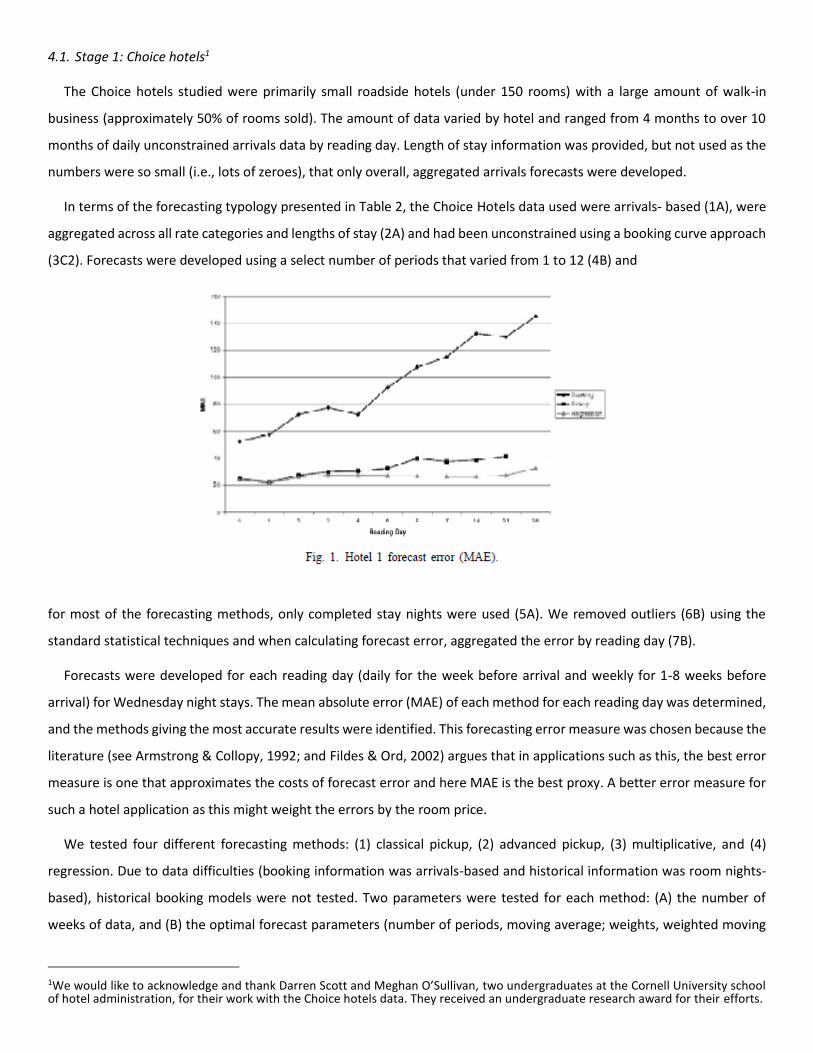
The number of weeks of data used in the training set to determine the parameter values was varied for each method to

determine the best amount of data to use (see Table 3) for each of four different hotel properties. Six weeks of data

produced the lowest error in the holdout sample for regression methods, 3 -6 weeks of data provided the best

performance for pickup methods, and 3 -5 weeks of data resulted in the best performance of the multiplicative forecasts.

For example, for the exponential smoothing method, suppose 6 weeks of data were used to identify the best value of a.

This parameter value was then held constant when forecasting for the observations in the holdout sample (week 7 and

beyond).

4.2. Stage 2: Marriott hotels data

Preliminary results from Choice Hotel data showed that the pickup and regression methods worked relatively well. To

validate and extend this finding, we obtained additional data from Marriott Hotels for two large business hotels without

a large amount of group business (less than 10%). The data contained unconstrained transient arrivals data on a daily basis

over a nearly 2-year period of time. The detailed arrivals data included the pattern of reservations booked at 16 different

reading days (84 days out, 70, 56, 42, 35, 28, 21, 14, 7, and daily to 0) for arrivals by length of stay (seven different

categories) and rate category (eight different categories). This meant that for any day-of-week, we had 101 observations

of the buildup in reservations for a given rate category and length of stay. Note: because of strong day-of-week seasonality,

it is standard practice in the hotel industry to only use Monday nights’ data to forecast other Mondays, only use Thursday

nights’ data to forecast other Thursdays, etc.

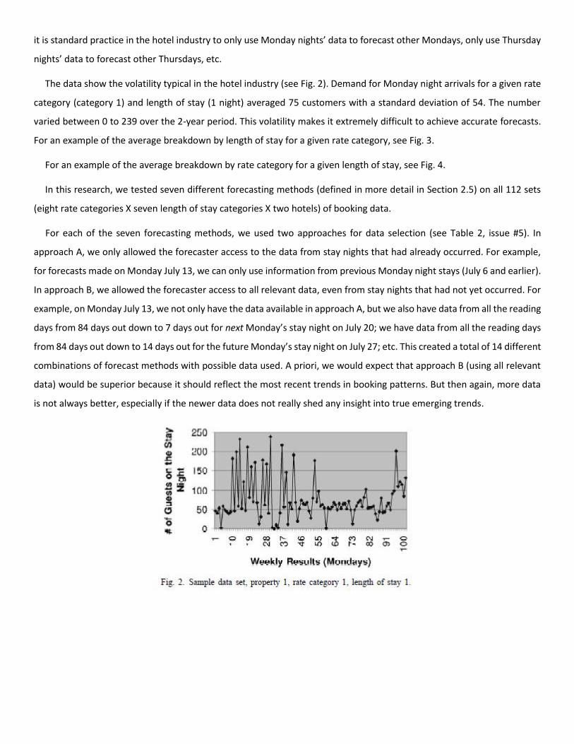
The data show the volatility typical in the hotel industry (see Fig. 2). Demand for Monday night arrivals for a given rate

category (category 1) and length of stay (1 night) averaged 75 customers with a standard deviation of 54. The number

varied between 0 to 239 over the 2-year period. This volatility makes it extremely difficult to achieve accurate forecasts.

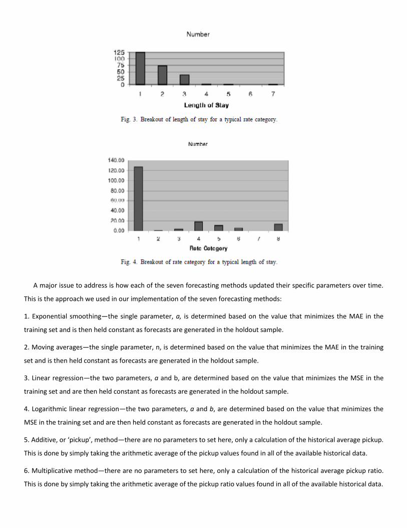
For an example of the average breakdown by length of stay for a given rate category, see Fig. 3.

For an example of the average breakdown by rate category for a given length of stay, see Fig. 4.

In this research, we tested seven different forecasting methods (defined in more detail in Section 2.5) on all 112 sets

(eight rate categories X seven length of stay categories X two hotels) of booking data.

For each of the seven forecasting methods, we used two approaches for data selection (see Table 2, issue #5). In

approach A, we only allowed the forecaster access to the data from stay nights that had already occurred. For example,

for forecasts made on Monday July 13, we can only use information from previous Monday night stays (July 6 and earlier).

In approach B, we allowed the forecaster access to all relevant data, even from stay nights that had not yet occurred. For

example, on Monday July 13, we not only have the data available in approach A, but we also have data from all the reading

days from 84 days out down to 7 days out for next Monday’s stay night on July 20; we have data from all the reading days

from 84 days out down to 14 days out for the future Monday’s stay night on July 27; etc. This created a total of 14 different

combinations of forecast methods with possible data used. A priori, we would expect that approach B (using all relevant

data) would be superior because it should reflect the most recent trends in booking patterns. But then again, more data

is not always better, especially if the newer data does not really shed any insight into true emerging trends.

A major issue to address is how each of the seven forecasting methods updated their specific parameters over time.

This is the approach we used in our implementation of the seven forecasting methods:

1. Exponential smoothing—the single parameter, a, is determined based on the value that minimizes the MAE in the

training set and is then held constant as forecasts are generated in the holdout sample.

2. Moving averages—the single parameter, n, is determined based on the value that minimizes the MAE in the training

set and is then held constant as forecasts are generated in the holdout sample.

3. Linear regression—the two parameters, a and b, are determined based on the value that minimizes the MSE in the

training set and are then held constant as forecasts are generated in the holdout sample.

4. Logarithmic linear regression—the two parameters, a and b, are determined based on the value that minimizes the

MSE in the training set and are then held constant as forecasts are generated in the holdout sample.

5. Additive, or ‘pickup’, method—there are no parameters to set here, only a calculation of the historical average pickup.

This is done by simply taking the arithmetic average of the pickup values found in all of the available historical data.

6. Multiplicative method—there are no parameters to set here, only a calculation of the historical average pickup ratio.

This is done by simply taking the arithmetic average of the pickup ratio values found in all of the available historical data.

7. Holt’s Double Exponential smoothing—the two parameters, a and ß, are determined based on the values that minimize

the MAE in the training set and are then held constant as forecasts are generated in the holdout sample.

In terms of the forecasting typology presented in Table 2, the Marriott Hotels project used data that was arrivals-based

(1A), were disaggregated by rate categories and by length of stay (2E) and had been unconstrained using denials data (3B).

Forecasts were developed using all periods (4A) and all forecasting methods were tested with both all data (5B) and only

completed stay nights (5A). Outliers were removed (6B) and forecast errors were averaged and reported over all reading

days (7C).

Forecasts were developed for each reading day. The mean absolute error (MAE) and mean absolute percentage error

(MAPE) of each method for each reading day was determined, and the methods giving the most accurate results (averaged

over all the reading days) were identified.

5. Results and discussion

Because of the large number of data sets for which forecasts were made, we will report the results on a summarized

basis even though the forecasting was done at the property/rate category/length of stay level (e.g., for property 1, rate

category 1, all seven lengths of stay (LOS) will be grouped into one summary chart showing the average MAE by forecasting

method for the set). The summary results for all eight rate categories are shown in Table 4 (the actual MAEs for each of

the 14 forecasting approaches are shown as Table 5) and Figs. 5 and 6 show sample graphs for two different rate

categories. The best method varied by property, rate category and length of stay, but the forecasting method which

minimized the MAE across all 112 data sets was 1a (exponential smoothing method using only completed stay night data),

and the method that minimized the MAPE was 5a (pickup method using only completed stay night data). Table 7

summarizes the percentage of the time that a particular forecast method was the best (i.e., lowest MAE) for a given

property/RC/LOS.

The most robust methods (as measured by the percentage of the cases that they had the lowest MAE) were exponential

smoothing (1a/b) and pickup (5a/b) methods with 33.3 and 25.1%, respectively. Next most robust were the moving

average (2a/b), Holt’s method (7a/b) and linear regression (3a/b) methods with 15.4, 12.9 and 10.9%, respectively.

Log linear methods (4a/b) and multiplicative methods (6a/b) performed poorly. Whether the methods used only

completed stay night data or all available stay nights (i.e., approach ‘A’ vs. ‘B’) did not seem to matter: about 52.5% of the

cases did better with approach A (only completed stay night data) and 47.5% did better with approach B (using all relevant

data). Furthermore, using the most robust method overall (exponential smoothing) does not seem to lead to much

deterioration if applied across hotel properties, rate categories and lengths of stay. These results are consistent with the

Makridakis et al. (1982) competition which found that moving averages and exponential smoothing methods were among

the most robust.

As a recommendation to hotel revenue managers, we would suggest the following:

A similar analysis to that presented here should be carried out on the hotel’s own data; differences exist across

companies and even across different properties within the same company.

Data: using completed stay night information is unlikely to lead to a deterioration in accuracy.

The choice of forecasting method: we would suggest any one of the five most robust methods (exponential

smoothing, pickup, moving average, Holt’s method and linear regression) or maybe even generate forecasts using

all five methods and then combine them in some way. (See Clemen (1989) for a good review of the literature on

combination forecasts.)

As Fildes and Lusk (1984) said, ‘‘no reasonable forecaster can identify the ‘best’ method from the various forecasting

competitions and adopt that method for his/her specific forecasting problem.... Typically, the forecaster should consider

a range of methods, and analyse their comparative performance over a random sample of those series of interest.’’ Future

research should include a study of combination forecasts using the five robust methods identified here to see what, if any,

additional forecast accuracy can be gained. Finally, a study of the optimal amount of historical data to use in setting the

forecast parameters would be helpful.

5.1. Note

The Marriott data can be made available to any interested researcher at the International Institute of Forecasters’

website or by contacting the lead author at his email address.

References

Adams, W., & Vodicka, M. (1987). Short-term forecasting of passenger demand and some applications in Qantas. In Proceedings of the 27 Annual AGIFORS Symposium. Armstrong, J. S., & Collopy, F. (1992). Error measures for generalizing about forecasting methods: empirical comparisons. International Journal of Forecasting, 8, 99-111.

Baker, T. K., & Collier, D. A. (1999). A comparative revenue analysis of hotel yield management heuristics. Decision Sciences, 30, 239-263.

Ben-Akiva, M. (1987). Improving airline passenger forecasts using reservation data. In Presentation at Fall ORSA/TIMS Conference. St. Louis.

Belobaba, P P (1985). TWA reservations analyses: demand distribution patterns. In MIT Flight Transportation Lab Report. Cambridge.

Clemen, R. T. (1989). Combining forecasts: a review and annotated bibliography. International Journal of Forecasting, 5, 559-584.

Duncanson, A. V (1974). Short-term forecasting. In Proceedings of the 14th Annual AGIFORS Symposium.

Fildes, R., & Lusk, E. J. (1984). The choice of a forecasting model. Omega, 12, 427-435.

Fildes, R., & Ord, K. (2002). Forecasting competitions—their role in improving forecasting practice and research. In Clements, M., & Hendry, D. (Eds.), A Companion to Economic Forecasting. Oxford: Blackwell.

Hanks, R. D. (1993). Revenue management at Marriott. In Proceedings of the IATA’s 5th International Revenue Management Conference, Montreal, Canada, pp. 246-282.

Hopperstad, C. (1995). An Alternative Detruncation Method. Boeing Commercial Aircraft Company Internal Document.

Kimes, S. E. (1999). Group forecasting accuracy for hotels. Journal of the Operational Research Society, 50(11), 11041110.

L’Heureux, E. (1986). A new twist in forecasting short-term passenger pickup. In Proceedings of the 26th Annual AGIFORS Symposium.

Lee, A.O. (1990). Airline Reservations Forecasting: Probabilistic and Statistical Models of the Booking Process. Flight Transportation Laboratory Report R90-5. Massachusetts Institute of Technology.

Littlewood, K. (1972). Forecasting and control of passenger bookings. In Proceedings of the 12th Annual AGIFORS Symposium.

Maddala, G. S. (1983). In Limited-Dependent and Qualitative Variables in Econometrics. Cambridge: Cambridge University Press.

Makridakis, S., Andersen, A., Carbone, R., Fildes, R., Hibon, M., Lewandowski, R., Newton, J., Parzen, E., & Winkler, R. (1982). The accuracy of extrapolation (time series) methods: results of a forecasting competition. Journal of Forecasting, 1, 111-153.

McCartney, S. (2000). In Airlines Find a Bag ofHigh-Tech Tricks to Keep Income Aloft, January Wall Street Journal, p. A1.

Orkin, E. (1998). Wishful thinking and rocket science: the essential matter of calculating unconstrained demand for revenue management. Cornell Hotel and Restaurant Administration Quarterly, 39, 15 -19.

Sa, J. (1987). Reservations forecasting in airline yield management. In MIT Flight Transportation Lab Report R87-1. Cambridge, MA.

Schneider, H. (1986). In Truncated and Censored Samples from Normal Populations. New York: Marcel Dekker.

Skwarek, D.K. (1996). Competitive Impacts of Yield Management System Components: Forecasting and Sell-Up Models. MIT Flight Transportation Lab Report R96-6.

Smith, B., & Penn, C. (1988). Analysis of alternate origindestination control strategies. In Proceedings of the 28th Annual AGIFORS Symposium.

Weatherford, L. R. (1997). A review of optimization modeling assumptions and their impact on revenue. In Presentation at Spring INFORMS Conference, San Diego, CA.

Weatherford, L. R. (1998). Forecasting issues in revenue management. In Presentation at Spring INFORMS Conference, Montreal, Canada.

Weatherford, L. R., Kimes, S. E. & Scott D. A. (2001). Forecasting for hotel revenue management: testing aggregation against disaggregation. Cornell Hotel and Restaurant Administration Quarterly. Forthcoming

Weatherford, L. R. & Polt, S. (2001). Better unconstraining of airline demand data in revenue management systems for improved forecast accuracy and greater revenues, unpublished manuscript in possession of the authors.

Wickham, R. R. (1995). Evaluation of forecasting techniques for short-term demand of air transportation. MIT Thesis: Flight Transportation Lab.

Zickus, J. (1998). Forecasting for Airline Network Revenue Management: Revenue and Competitive Impacts. MIT Flight Transportation Lab Report R98-4.

Biographies: Larry WEATHERFORD is an Associate Professor at the University of Wyoming. He holds a Ph.D. from the Darden Graduate Business School, University of Virginia. Larry teaches undergraduate and MBA classes in Operations Management and Quantitative Methods. He has received several Outstanding Teaching Awards from the College of Business and the University of Wyoming. He also has a best-selling textbook, Decision Modeling with Microsoft Excel, published by Prentice Hall, Inc. in 2001. He has published 17 articles in such journals as Operations Research, Decision Sciences, Naval Research Logistics, Transportation Science, Omega, International Journal of Technology Management, Cornell Hotel and Restaurant Administration Quarterly, Journal of Combinatorial Optimization, International Journal of Operations and Quantitative Management and OR/MS Today and presented 51 papers on five different continents to professional organizations. He has consulted with such major corporations as American Airlines, Northwest Airlines, Lufthansa German Airlines, Swissair, Scandinavian Airlines, Air New Zealand, South African Airways, Unisys Corporation, Walt Disney World, Hilton Hotels and Choice Hotels, as well as many other smaller corporations.

Sheryl E. KIMES is Professor of Operations Management in the School of Hotel Administration at Cornell University. She holds a Ph.D. in operations management from the University of TexasAustin. She specializes in revenue management and has worked with a variety of industries around the world. Her research has appeared in Interfaces, Journal of Operations Management, Journal of Service Research and other journals.