IN DEGREE PROJECT ELECTRICAL ENGINEERING,SECOND CYCLE, 30 CREDITS

, STOCKHOLM SWEDEN 2016

A comparison of 5G candidate waveforms subject to phase noise impairment at mm-wave frequencies

VICENT MOLÉS CASES

KTH ROYAL INSTITUTE OF TECHNOLOGYSCHOOL OF ELECTRICAL ENGINEERING

Acknowledgments

I would specially like to express my sincere gratitude to my Ericsson’s supervisor Ali Zaidi forall his help, advise and encouragements during the thesis work, without whom I would not havedone this thesis.

I would also like to thank the Radio Access Technologies Department of Ericsson Research forgiving me the opportunity to carry out this thesis, providing all the support needed.

I am very grateful to Gema Pinero and Tobias Oechtering for being my supervisors at UPVand KTH respectively, giving always all the needed advise.

My friends and master thesis mates Adrian, Matyas and Gabri deserve here a special recogni-tion too, since the talks and moments with them definitely inspired my thesis.

I can not forget my lifelong friends, who provided some badly needed distraction from allwork-related thoughts; my parents, who always supported me in my life and work; my sister,who provided a very useful help and Marisol, who gave me very useful advice and inspiration.Finally, I would like to thank Marıa Jose for her unconditional support and love.

Abstract

Frequencies above 6 GHz are being considered by mobile communication industry for the deploy-ment of future 5G networks. Large channel bandwidths above 6 GHz are likely to be used to servediverse use cases and meet extreme user requirements. However in the higher carrier frequencies,especially the millimeter-wave frequencies (above 30 GHz), there can be severe degradations inthe transmitted and received signals due to Radio-Frequency (RF) impairments such as phasenoise introduced by the local oscillators. 5G radio interface, operating higher carrier frequencies,has to be robust against phase noise. In this thesis, the effect of phase noise has been investigatedfor three different multi-carrier waveforms, namely Orthogonal Frequency Division Multiplexing(OFDM), Offset QAM Filter-Bank Multi-Carrier (OQAM-FBMC) and QAM Filter-Bank Multi-Carrier (QAM-FBMC). These waveforms have been considered as potential candidates for 5Gradio interface. We develop analytical tools to evaluate the performance of these three waveformssubject to phase noise in terms of Signal-to-Interference Ratio (SIR). The derived tools can beused to obtain SIR under any phase noise model with a known phase noise spectral density.We have used a specific phase noise model (the mmMagic phase noise model) in our waveformevaluations and comparisons at three different carrier frequencies: 6 GHz, 28 GHz, and 82 GHz.The theoretical results are further verified using Monte Carlo evaluations for SIR and SymbolError Rate (SER). The evaluation results reveal that OFDM is relatively more robust to phasenoise than OQAM-FBMC and QAM-FBMC. It has been also observed that the choice of theoverlapping factor in FBMC based waveforms can play a role in the performance. For the givenphase noise model, OFDM has been observed to be robust to phase noise even at very highfrequency (up to 82 GHz), which makes it a strong candidate for 5G radio interface.

Sammanfattning

Frekvenser over 6 GHz overvags av mobilkommunikationsbranschen for utbyggnaden av framtida5G natverk. Men i frekvenser over 30 GHz kan det finnas allvarliga forsamringar i signalernapagrund av fasbruset som infors genom lokala oscillatorer. Rapporten presenterar effekten avfasbruset undersokts for tre olika multi-carrier vagformer, namligen Orthogonal Frequency Divi-sion Multiplexing (OFDM), Offset QAM Filter-Bank Multi-Carrier (OQAM-FBMC), och QAMFilter-Bank Multi- Carrier (QAM-FBMC). Vi utvecklar analysverktyg for att utvardera ochjamfora prestanda for dessa tre vagformer som omfattas av fasbrus vid 6 GHz, 28 GHz, och82 GHz. De teoretiska resultaten verifieras ytterligare med hjalp av Monte Carlo-simuleringar.Utvarderingsresultaten visar att OFDM ar relativt mer robust att fasbrus an OQAM-FBMC ochQAM-FBMC.

Contents

Index 2

1 Introduction 31.1 Motivation . . . . . . . . . . . . . . . . . . . . . . . . . . . . . . . . . . . . . . . 31.2 Previous work . . . . . . . . . . . . . . . . . . . . . . . . . . . . . . . . . . . . . . 31.3 Goals . . . . . . . . . . . . . . . . . . . . . . . . . . . . . . . . . . . . . . . . . . 41.4 Societal Aspects . . . . . . . . . . . . . . . . . . . . . . . . . . . . . . . . . . . . 41.5 Tasks sequence . . . . . . . . . . . . . . . . . . . . . . . . . . . . . . . . . . . . . 41.6 Outline . . . . . . . . . . . . . . . . . . . . . . . . . . . . . . . . . . . . . . . . . 51.7 Acronyms and Nomenclature . . . . . . . . . . . . . . . . . . . . . . . . . . . . . 6

2 Background 82.1 Multi-Carrier Modulations . . . . . . . . . . . . . . . . . . . . . . . . . . . . . . . 8

2.1.1 OFDM . . . . . . . . . . . . . . . . . . . . . . . . . . . . . . . . . . . . . 112.1.2 QAM-FBMC . . . . . . . . . . . . . . . . . . . . . . . . . . . . . . . . . . 142.1.3 OQAM-FBMC . . . . . . . . . . . . . . . . . . . . . . . . . . . . . . . . . 17

2.2 Phase noise . . . . . . . . . . . . . . . . . . . . . . . . . . . . . . . . . . . . . . . 202.2.1 Effect of phase noise in a generic signal . . . . . . . . . . . . . . . . . . . 22

3 OFDM 233.1 Continuous time Modulated and Demodulated signal . . . . . . . . . . . . . . . . 233.2 Continuous time Demodulated signal subject to phase noise . . . . . . . . . . . . 24

3.2.1 Interference power . . . . . . . . . . . . . . . . . . . . . . . . . . . . . . . 253.2.2 Signal-to-Interference Ratio due to phase noise . . . . . . . . . . . . . . . 26

3.3 Discrete time Modulated and Demodulated signal . . . . . . . . . . . . . . . . . . 263.4 Discrete time Demodulated signal subject to phase noise . . . . . . . . . . . . . . 27

3.4.1 Interference power . . . . . . . . . . . . . . . . . . . . . . . . . . . . . . . 283.4.2 Signal-to-Interference Ratio due to phase noise . . . . . . . . . . . . . . . 29

3.5 Weighting functions . . . . . . . . . . . . . . . . . . . . . . . . . . . . . . . . . . 293.5.1 Shape analysis . . . . . . . . . . . . . . . . . . . . . . . . . . . . . . . . . 303.5.2 Comparison between continuous and discrete time . . . . . . . . . . . . . 32

3.6 Signal-to-Interference Ratio evaluations . . . . . . . . . . . . . . . . . . . . . . . 353.6.1 Theoretical results . . . . . . . . . . . . . . . . . . . . . . . . . . . . . . . 353.6.2 Simulations results . . . . . . . . . . . . . . . . . . . . . . . . . . . . . . . 36

3.7 Symbol Error Rate simulations . . . . . . . . . . . . . . . . . . . . . . . . . . . . 37

1

4 QAM-FBMC 404.1 Modulated and demodulated signal . . . . . . . . . . . . . . . . . . . . . . . . . . 404.2 Demodulated signal subject to phase noise . . . . . . . . . . . . . . . . . . . . . . 41

4.2.1 Interference power . . . . . . . . . . . . . . . . . . . . . . . . . . . . . . . 434.2.2 Signal-to-Interference Ratio . . . . . . . . . . . . . . . . . . . . . . . . . . 45

4.3 Weighting functions . . . . . . . . . . . . . . . . . . . . . . . . . . . . . . . . . . 454.3.1 Shape analysis . . . . . . . . . . . . . . . . . . . . . . . . . . . . . . . . . 46

4.4 Signal-to-Interference Ratio evaluations . . . . . . . . . . . . . . . . . . . . . . . 48

5 OQAM-FBMC 515.1 Modulated and Demodulated signal . . . . . . . . . . . . . . . . . . . . . . . . . 515.2 Demodulated signal subject to phase noise . . . . . . . . . . . . . . . . . . . . . . 52

5.2.1 Interference power . . . . . . . . . . . . . . . . . . . . . . . . . . . . . . . 545.2.2 Signal-to-Interference Ratio . . . . . . . . . . . . . . . . . . . . . . . . . . 56

5.3 Weighting functions . . . . . . . . . . . . . . . . . . . . . . . . . . . . . . . . . . 575.3.1 Shape analysis . . . . . . . . . . . . . . . . . . . . . . . . . . . . . . . . . 57

5.4 Signal-to-Interference Ratio evaluations . . . . . . . . . . . . . . . . . . . . . . . 605.4.1 Theoretical results . . . . . . . . . . . . . . . . . . . . . . . . . . . . . . . 605.4.2 Simulation results . . . . . . . . . . . . . . . . . . . . . . . . . . . . . . . 64

5.5 Symbol Error Rate evaluations . . . . . . . . . . . . . . . . . . . . . . . . . . . . 66

6 Comparison of waveforms subject to phase noise 68

7 Conclusions and future work 737.1 Conclusions . . . . . . . . . . . . . . . . . . . . . . . . . . . . . . . . . . . . . . . 737.2 Future work . . . . . . . . . . . . . . . . . . . . . . . . . . . . . . . . . . . . . . . 74

Appendices 75

A OFDM Derivations 76A.1 Derivation of E

[|ϕi,l|2

]. . . . . . . . . . . . . . . . . . . . . . . . . . . . . . . . 76

A.2 Derivation of E[|ϕi,l|2

]. . . . . . . . . . . . . . . . . . . . . . . . . . . . . . . . 78

B QAM-FBMC Derivations 80B.1 Derivation of |λi,l,d|2 . . . . . . . . . . . . . . . . . . . . . . . . . . . . . . . . . . 80

B.2 Derivation of E[|βi,l,d|2

]. . . . . . . . . . . . . . . . . . . . . . . . . . . . . . . . 82

C OQAM-FBMC Derivations 83C.1 Derivation of |γi,l,d|2 . . . . . . . . . . . . . . . . . . . . . . . . . . . . . . . . . . 83

C.2 Derivation of E[|ρi,l,d|2

]. . . . . . . . . . . . . . . . . . . . . . . . . . . . . . . . 86

2

Chapter 1

Introduction

1.1 Motivation

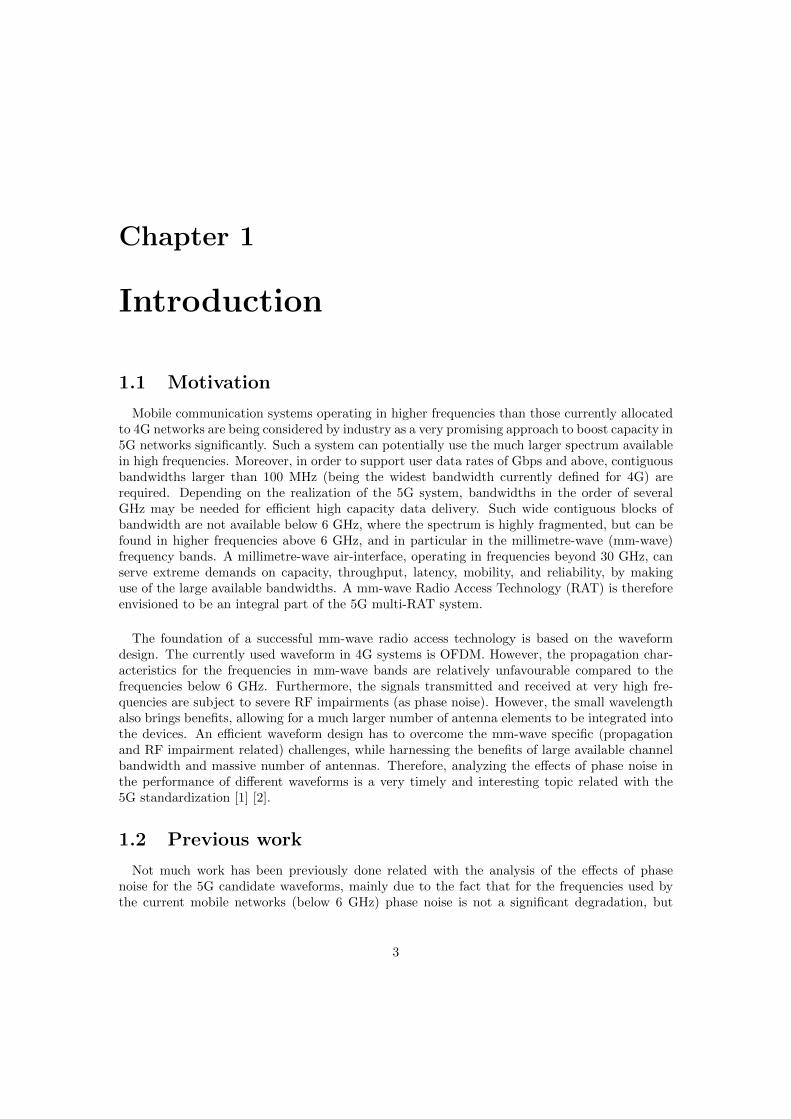
Mobile communication systems operating in higher frequencies than those currently allocatedto 4G networks are being considered by industry as a very promising approach to boost capacity in5G networks significantly. Such a system can potentially use the much larger spectrum availablein high frequencies. Moreover, in order to support user data rates of Gbps and above, contiguousbandwidths larger than 100 MHz (being the widest bandwidth currently defined for 4G) arerequired. Depending on the realization of the 5G system, bandwidths in the order of severalGHz may be needed for efficient high capacity data delivery. Such wide contiguous blocks ofbandwidth are not available below 6 GHz, where the spectrum is highly fragmented, but can befound in higher frequencies above 6 GHz, and in particular in the millimetre-wave (mm-wave)frequency bands. A millimetre-wave air-interface, operating in frequencies beyond 30 GHz, canserve extreme demands on capacity, throughput, latency, mobility, and reliability, by makinguse of the large available bandwidths. A mm-wave Radio Access Technology (RAT) is thereforeenvisioned to be an integral part of the 5G multi-RAT system.

The foundation of a successful mm-wave radio access technology is based on the waveformdesign. The currently used waveform in 4G systems is OFDM. However, the propagation char-acteristics for the frequencies in mm-wave bands are relatively unfavourable compared to thefrequencies below 6 GHz. Furthermore, the signals transmitted and received at very high fre-quencies are subject to severe RF impairments (as phase noise). However, the small wavelengthalso brings benefits, allowing for a much larger number of antenna elements to be integrated intothe devices. An efficient waveform design has to overcome the mm-wave specific (propagationand RF impairment related) challenges, while harnessing the benefits of large available channelbandwidth and massive number of antennas. Therefore, analyzing the effects of phase noise inthe performance of different waveforms is a very timely and interesting topic related with the5G standardization [1] [2].

1.2 Previous work

Not much work has been previously done related with the analysis of the effects of phasenoise for the 5G candidate waveforms, mainly due to the fact that for the frequencies used bythe current mobile networks (below 6 GHz) phase noise is not a significant degradation, but

3

also because some of the waveforms proposed for 5G have been presented recently and notmuch previous research related with them has been done. In [3] the effects of phase noise incontinuous time OFDM were presented and the concept of weighting functions (what will belater on explained) was introduced. In [4] the effects of phase noise in OFDM were studiedfor different phase noise models and different receiver types (coherent and differential receiver).In [5] expressions for the power of the interferences produced by phase noise in OQAM-FBMCwere presented, however without taking into account the effects of the intrinsic interferences thataffect OQAM-FBMC.

1.3 Goals

The main goal of this master’s thesis is to analyse and compare the effects of phase noise inOFDM, QAM-FBMC and OQAM-FBMC for the mm-wave band. The mentioned waveforms arethree of the most promising candidate Multi-Carrier Modulation (MCM) for 5G. The comparisonshould give a clear idea of which waveform offers better performance in the presence of phasenoise for frequencies above 6 GHz. The performance is evaluated using as metrics the Signal-to-Interference Ratio (SIR) and the Symbol Error Rate (SER).

In order to carry out the comparison, we derive a method to evaluate the performance of thedifferent MCM subject to phase noise. The most significant strength of the developed method isthat it provides tools to analyse the effects of phase noise for any oscillator whose Power SpectralDensity (PSD) is known and with any set of waveform parameters (as the signal bandwidthor the symbol length). So the method can be used to compare the performance of the threewaveforms subject to phase noise for any case, which is a very helpful tool when deciding whichis the best waveform for 5G in terms of robustness against phase noise.

1.4 Societal Aspects

Usually people think that the main difference between 4G and 5G is only related with trans-mission speed. However, 5G will not only offer higher transmission speed than 4G, it is supposedto offer other important properties, as higher energy efficiency and a big variety of services andcases (as machine-to-machine and vehicle-to-vehicle). These new properties will help to the de-velopment of different innovations that will have high impact in the society, as the drive-less car,the smart cities, the remote surgery and many other. One important aspect in order to achievethese innovations is the study of the communications in the mm-Wave band. Therefore, thestudy of the effects of phase noise in the communications in the mm-Wave band is a key aspectin order to achieve the previous mention innovations.

1.5 Tasks sequence

In this section we present the time distribution of the different stages in which the thesis hasbeen divided:

• Stage 1: Bibliographic research and state of the art about 5G, MCM, OFDM, QAM-FBMC,OQAM-FBMC and phase noise, in order to get a solid background regarding the thesistopics.

4

• Stage 2: Study of the effects of phase noise in OFDM, deriving tools that allow us toevaluate the SIR theoretically. Perform simulations to check the accuracy of the theoreticalresults.

• Stage 3: Analysis of the effects of phase noise in QAM-FBMC, deriving tools that allow usto evaluate the SIR theoretically.

• Stage 4: Examination of the effects of phase noise in OQAM-FBMC, deriving tools thatallow us to evaluate the SIR theoretically. Performance of simulations to check the accuracyof the theoretical results.

• Stage 5: Performance of simulations to study the effect of phase noise in the SER for thedifferent waveforms.

• Stage 6: Analysis of the results and report writing.

• Stage 7: Preparation of the master’s thesis presentation, including the slides elaboration.

1.6 Outline

The rest of the report is organized as follows:

• Chapter 2 presents the theoretical background needed to follow the rest of the thesis.Concretely, concepts about MCM, OFDM, QAM-FBMC, OQAM-FBMC and phase noiseare discussed.

• Chapter 3, 4 and 5 contain the derivations needed to study the effect of phase noise inOFDM, QAM-FBMC and OQAM-FBMC respectively.

• Chapter 6 presents the comparison of the results obtained for the three waveforms.

• Chapter 7 summarizes the thesis, presents the conclusions and gives some ideas of likelyfuture work.

• Appendix A, B and C contain derivations related with Chapter 3, 4 and 5 respectively.

5

1.7 Acronyms and Nomenclature

Acronyms

Acronym DescriptionAWGN Additive White Gaussian NoiseCP Cyclic PrefixDTFT Discrete Time Fourier TransformFFT Fast Fourier TransformFIR Finite impulse responseICI Inter-Carrier InterferenceIDTFT Inverse Discrete Time Fourier TransformIFFT Inverse Fast Fourier TransformISI Inter-Symbol InterferenceLPF Low Pass FilterLTE Long Term EvolutionMCM Multi-Carrier ModulationOFDM Orthogonal Frequency Division MultiplexingOQAM-FBMC Offset Quadrature Amplitude Modulation - Filter Bank Multi-CarrierPLL Phase-Locked LoopPN-CPE Phase Noise - Common Phase ErrorPN-ICI Phase Noise - Inter-Carrier InterferencePN-ISI Phase Noise - Inter-Symbol InterferencePSD Power Spectral DensityQAM-FBMC Quadrature Amplitude Modulation - Filter Bank Multi-CarrierRAT Radio Access TechnologySCM Single-Carrier ModulationSER Symbol Error RateS-ICI Self - Inter-Carrier InterferenceSIR Signal-to-Interference RatioS-ISI Self - Inter-Symbol InterferenceSNR Signal-to-Noise RatioVCO Voltage Controlled OscillatorWSS Wide-Sense Stationary Stochastic

6

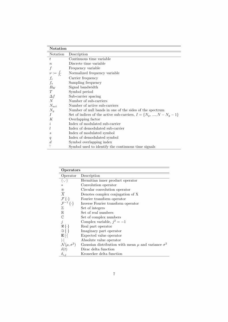
Notation

Notation Descriptiont Continuous time variablen Discrete time variablef Frequency variable

ν := ffs

Normalized frequency variable

fc Carrier frequencyfs Sampling frequencyBW Signal bandwidthT Symbol period∆f Sub-carrier spacingN Number of sub-carriersNact Number of active sub-carriersNg Number of null bands in one of the sides of the spectrumI Set of indices of the active sub-carriers, I = Ng, ..., N −Ng − 1K Overlapping factori Index of modulated sub-carrierl Index of demodulated sub-carriers Index of modulated symbolq Index of demodulated symbold Symbol overlapping index· Symbol used to identify the continuous time signals

Operators

Operator Description〈·, ·〉 Hermitian inner product operator∗ Convolution operator~ Circular convolution operatorX Denotes complex conjugation of XF · Fourier transform operatorF−1 · Inverse Fourier transform operatorZ Set of integersR Set of real numbersC Set of complex numbersj Complex variable, j2 = −1<· Real part operator=· Imaginary part operatorE [·] Expected value operator|·| Absolute value operatorN (µ, σ2) Gaussian distribution with mean µ and variance σ2

δ(t) Dirac delta functionδi,j Kronecker delta function

7

Chapter 2

Background

In this chapter we provide a brief discussion of the essential theoretical background neededthroughout the thesis. First the concept of Multi-Carrier Modulations (MCM) is presented,followed by a detailed explanation of the different properties for the three MCM studied in thisthesis (OFDM, QAM-FBMC and OQAM-FBMC). Finally, the concept of phase noise and itseffects on a modulated signal are presented.

2.1 Multi-Carrier Modulations

In classical Single-Carrier modulations (SCM), the information is transmitted over one singlecarrier frequency using high transmission rates, i.e., wide signal bandwidth and short symbolduration. Multi-Carrier Modulations (MCM) is a group of waveforms in which the informationis split and transmitted simultaneously over different carrier frequencies (called sub-carriers) eachone with low transmission rates (compared to SCM), i.e., narrow sub-carrier bandwidth and longsymbol duration [6, pp. 27-30].

The main advantage of MCM over SCM which makes them preferred for high speed wirelesstransmissions is their robustness against frequency selective fading channels. Their robustnessis explained because a selective fading channel can be divided into parallel frequency flat fadingnarrow subchannels in MCM (one for each sub-carrier). This effect can be seen in Figure 2.1.Thus, the channel equalization for MCM is an easy process performed in the frequency domainseparately for each subchannel. Contrary, in SCM subject to a frequency selective fading channelthe equalization is performed in the time domain using complex procedures.

f

BW

(a) Selective Fading Channel

BW

f

∆f

(b) Flat Fading Subchannels

Figure 2.1: Effect of dividing a selective fading channel in narrow subchannels.

8

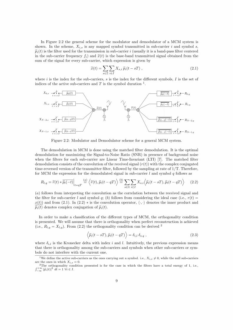
In Figure 2.2 the general scheme for the modulator and demodulator of a MCM system isshown. In the scheme, Xi,s is any mapped symbol transmitted in sub-carrier i and symbol s,pi(t) is the filter used for the transmission in sub-carrier i (usually it is a band-pass filter centeredin the sub-carrier frequency fi) and x(t) is the base-band transmitted signal obtained from thesum of the signal for every sub-carrier, which expression is given by

x(t) =∑

s∈Z

∑

i∈IXs,i pi(t− sT ) , (2.1)

where i is the index for the sub-carriers, s is the index for the different symbols, I is the set ofindices of the active sub-carriers and T is the symbol duration 1.

⊕

p0(t)

p1(t)

pN−2(t)

pN−1(t)

⊕

p0(−t)

p1(−t)

pN−2(−t)

pN−1(−t)

x(t) r(t)

X0,s

X1,s

XN−2,s

XN−1,s

t = s T

t = s T

t = s T

t = s T

t = q T

t = q T

t = q T

t = q T

R0,q

R1,q

RN−2,q

RN−1,q

⊗

fc

⊗

fc

Figure 2.2: Modulator and Demodulator scheme for a general MCM system.

The demodulation in MCM is done using the matched filter demodulation. It is the optimaldemodulation for maximizing the Signal-to-Noise Ratio (SNR) in presence of background noisewhen the filters for each sub-carrier are Linear Time-Invariant (LTI) [7]. The matched filterdemodulation consists of the convolution of the received signal (r(t)) with the complex conjugatedtime-reversed version of the transmitter filter, followed by the sampling at rate of 1/T. Therefore,for MCM the expression for the demodulated signal in sub-carrier l and symbol q follows as

Rl,q = r(t) ∗ pl(−t)∣∣∣t=qT

(a)=⟨r(t), pl(t− qT )

⟩(b)=∑

s∈Z

∑

i∈IXs,i

⟨pi(t− sT ), pl(t− qT )

⟩(2.2)

(a) follows from interpreting the convolution as the correlation between the received signal andthe filter for sub-carrier l and symbol q; (b) follows from considering the ideal case (i.e., r(t) =x(t)) and from (2.1). In (2.2) ∗ is the convolution operator, 〈·, ·〉 denotes the inner product andpi(t) denotes complex conjugation of pi(t).

In order to make a classification of the different types of MCM, the orthogonality conditionis presented. We will assume that there is orthogonality when perfect reconstruction is achieved(i.e., Rl,q = Xl,q). From (2.2) the orthogonality condition can be derived 2

⟨pi(t− sT ), pl(t− qT )

⟩= δi,l δs,q , (2.3)

where δi,l is the Kronecker delta with index i and l. Intuitively, the previous expression meansthat there is orthogonality among the sub-carriers and symbols when other sub-carriers or sym-bols do not interfere with the current one.

1We define the active sub-carriers as the ones carrying out a symbol. i.e., Xi,s 6= 0, while the null sub-carriersare the ones in which Xi,s = 0.

2The orthogonality condition presented is for the case in which the filters have a total energy of 1, i.e.,∫+∞−∞ |pi(t)|

2 dt = 1 ∀i ∈ I.

9

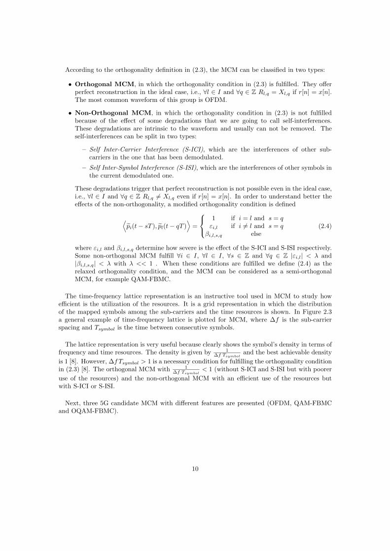
According to the orthogonality definition in (2.3), the MCM can be classified in two types:

• Orthogonal MCM, in which the orthogonality condition in (2.3) is fulfilled. They offerperfect reconstruction in the ideal case, i.e., ∀l ∈ I and ∀q ∈ Z Rl,q = Xl,q if r[n] = x[n].The most common waveform of this group is OFDM.

• Non-Orthogonal MCM, in which the orthogonality condition in (2.3) is not fulfilledbecause of the effect of some degradations that we are going to call self-interferences.These degradations are intrinsic to the waveform and usually can not be removed. Theself-interferences can be split in two types:

– Self Inter-Carrier Interference (S-ICI), which are the interferences of other sub-carriers in the one that has been demodulated.

– Self Inter-Symbol Interference (S-ISI), which are the interferences of other symbols inthe current demodulated one.

These degradations trigger that perfect reconstruction is not possible even in the ideal case,i.e., ∀l ∈ I and ∀q ∈ Z Rl,q 6= Xl,q even if r[n] = x[n]. In order to understand better theeffects of the non-orthogonality, a modified orthogonality condition is defined

⟨pi(t− sT ), pl(t− qT )

⟩=

1 if i = l and s = qεi,l if i 6= l and s = q

βi,l,s,q else(2.4)

where εi,l and βi,l,s,q determine how severe is the effect of the S-ICI and S-ISI respectively.Some non-orthogonal MCM fulfill ∀i ∈ I, ∀l ∈ I, ∀s ∈ Z and ∀q ∈ Z |εi,l| < λ and|βi,l,s,q| < λ with λ << 1 . When these conditions are fulfilled we define (2.4) as therelaxed orthogonality condition, and the MCM can be considered as a semi-orthogonalMCM, for example QAM-FBMC.

The time-frequency lattice representation is an instructive tool used in MCM to study howefficient is the utilization of the resources. It is a grid representation in which the distributionof the mapped symbols among the sub-carriers and the time resources is shown. In Figure 2.3a general example of time-frequency lattice is plotted for MCM, where ∆f is the sub-carrierspacing and Tsymbol is the time between consecutive symbols.

The lattice representation is very useful because clearly shows the symbol’s density in terms offrequency and time resources. The density is given by 1

∆f Tsymboland the best achievable density

is 1 [8]. However, ∆f Tsymbol > 1 is a necessary condition for fulfilling the orthogonality conditionin (2.3) [8]. The orthogonal MCM with 1

∆f Tsymbol< 1 (without S-ICI and S-ISI but with poorer

use of the resources) and the non-orthogonal MCM with an efficient use of the resources butwith S-ICI or S-ISI.

Next, three 5G candidate MCM with different features are presented (OFDM, QAM-FBMCand OQAM-FBMC).

10

f

tTSymbol

∆f

Symbol

Figure 2.3: Time-Frequency lattice representation for MCM.

2.1.1 OFDM

Orthogonal Frequency Division Multiplexing (OFDM) is the most popular and used MCM.The scheme for the modulator and the demodulator of an OFDM system is shown in Figure 2.4,where each sub-carrier carries a symbol Xi,s ∈ C.

ej2πf0t

ej2πf1t

ej2πfN−1t

ej2πfN−2t

⊗

⊗

⊗

⊗

⊕

p(t)

p(t)

p(t)

p(t)

X0,s

X1,s

XN−2,s

XN−1,s

e−j2πf0t

⊗

⊕

p(−t) R0,q

e−j2πf1t

⊗ p(−t) R1,q

e−j2πfN−2t

⊗ p(−t) RN−2,q

e−j2πfN−1t

⊗ p(−t) RN−1,q

t = sT

t = sT

t = sT

t = sT

t = qT

t = qT

t = qT

t = qT

⊗

fc fc

⊗

Figure 2.4: Continuous time OFDM Modulator and Demodulator.

If one compares Figure 2.4 and Figure 2.2, it is obvious that in OFDM the filter for eachsub-carrier is a frequency shift version of a base filter (p(t)), so it is defined as

pi(t) := p(t) ej2πfit , (2.5)

where p(t) is a rectangular filter with length T and fi is the frequency for sub-carrier i. The

11

base filter is defined as

p(t) :=

1√T

if 0 ≤ t ≤ T0 else

, (2.6)

in which the amplitude 1√T

is used to achieve a total energy of 1 for the base filter, i.e.,∫ +∞−∞ |p(t)|

2dt = 1.

Next, the orthogonality for OFDM is discussed. One important fact that has to be takeninto consideration is that in OFDM different symbols do not overlap each other. Therefore, noS-ISI effect appears and the orthogonality condition in (2.3) can be simplified by removing thecondition related with the symbol index (which is always true for OFDM), obtaining

⟨pi(t), pl(t)

⟩= δi,l (2.7)

From (2.7), the orthogonality for OFDM is studied

〈pi(t), pl(t)〉 =

∫ T

0

pi(t) pl(t) dt

=

∫ T

0

p(t) ej2πfit p(t) e−j2πflt dt

=

∫ T

0

ej2π(fi−fl)t dt

From the previous expression, the relation between sub-carriers needed to fulfill the orthogonalitycondition in (2.7) (and avoid S-ICI) can be deduced

fi − fl =i− lT

= (i− l) ∆f ,

in which ∆f is the sub-carrier spacing, ∆f := 1T . Therefore, OFDM is an orthogonal MCM

when the sub-carrier spacing is equal to the inverse of the symbol period. Finally, taking intoaccount the orthogonality condition the expression for the filter in sub-carrier i is given by

pi(t) = p(t) ej2πiT t (2.8)

In Figure 2.5 the shape of the frequency response for three orthogonal sub-carriers is rep-resented. The filter used for each sub-carrier has a rectangular impulse response of length T .Therefore, its frequency response has a sinc shape with null values in increments of ∆f = 1

T ,avoiding S-ICI.

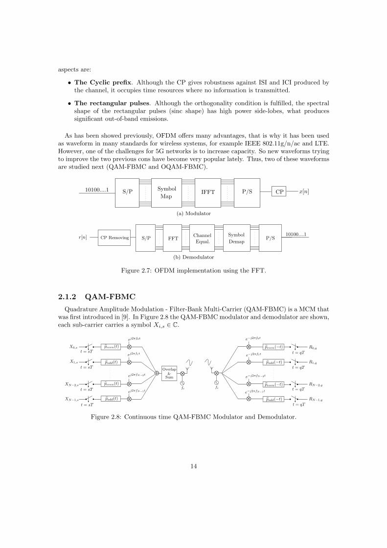
Another important characteristic of OFDM is Cyclic Prefix (CP). It is a repeated version ofthe last TCP seconds of the OFDM symbol in its beginning. The main goal of the CP is toavoid the ISI produced by channel multi-paths and keeping the orthogonality among sub-carriers(avoiding ICI). ISI and ICI produced by the channel are avoided when the spread delay of thechannel is shorter than the duration of the CP. If the spread delay is longer than the CP, ISIappears and the orthogonality among sub-carriers is lost.

In Figure 2.6 the lattice representation for OFDM has been plotted. The symbol density forOFDM is T

T+TCP< 1, it reflects that OFDM does not offer the most efficient use of the resources.

12

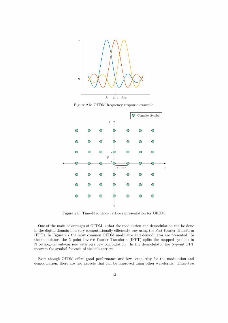
fi fi+1 fi+2

0

1

Figure 2.5: OFDM frequency response example.

f

tT + TCP

1T

Complex Symbol

Figure 2.6: Time-Frequency lattice representation for OFDM.

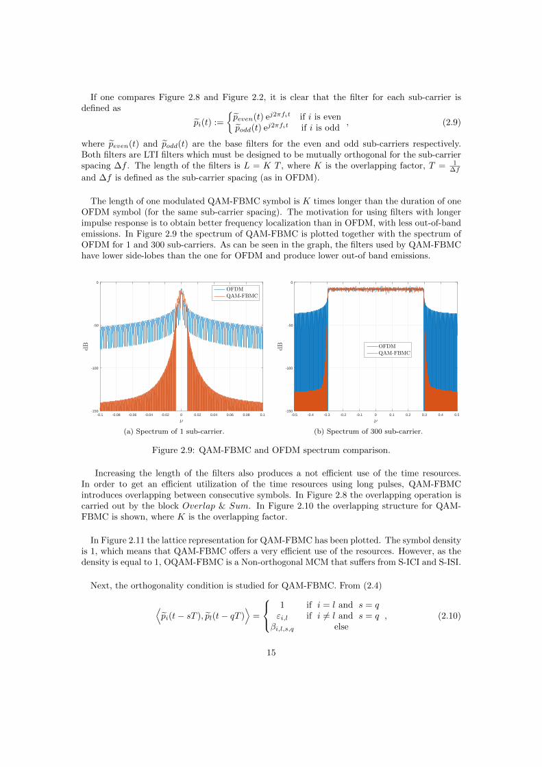
One of the main advantages of OFDM is that the modulation and demodulation can be donein the digital domain in a very computationally efficiently way using the Fast Fourier Transform(FFT). In Figure 2.7 the most common OFDM modulator and demodulator are presented. Inthe modulator, the N-point Inverse Fourier Transform (IFFT) splits the mapped symbols inN orthogonal sub-carriers with very few computation. In the demodulator the N-point FFTrecovers the symbol for each of the sub-carriers.

Even though OFDM offers good performance and low complexity for the modulation anddemodulation, there are two aspects that can be improved using other waveforms. These two

13

aspects are:

• The Cyclic prefix. Although the CP gives robustness against ISI and ICI produced bythe channel, it occupies time resources where no information is transmitted.

• The rectangular pulses. Although the orthogonality condition is fulfilled, the spectralshape of the rectangular pulses (sinc shape) has high power side-lobes, what producessignificant out-of-band emissions.

As has been showed previously, OFDM offers many advantages, that is why it has been usedas waveform in many standards for wireless systems, for example IEEE 802.11g/n/ac and LTE.However, one of the challenges for 5G networks is to increase capacity. So new waveforms tryingto improve the two previous cons have become very popular lately. Thus, two of these waveformsare studied next (QAM-FBMC and OQAM-FBMC).

10100....1 S/P Symbol

MapIFFT P/S CP x[n]

(a) Modulator

10100....1S/P

ChannelEqual.

FFT P/SCP RemovingDemap

r[n] Symbol

(b) Demodulator

Figure 2.7: OFDM implementation using the FFT.

2.1.2 QAM-FBMC

Quadrature Amplitude Modulation - Filter-Bank Multi-Carrier (QAM-FBMC) is a MCM thatwas first introduced in [9]. In Figure 2.8 the QAM-FBMC modulator and demodulator are shown,each sub-carrier carries a symbol Xi,s ∈ C.

peven(t)

ej2πf0t

t = sT

podd(t)

ej2πf1t

ej2πfN−1t

podd(t)

peven(t)

ej2πfN−2t

Overlap&

Sum

⊗

⊗

⊗

⊗

⊕

X0,s

XN−1,s

XN−2,s

X1,s

peven(−t)

t = qT

podd(−t)

⊗R0,q

RN−1,q

RN−2,q

R1,q⊗

⊗

⊗

peven(−t)

podd(−t)

t = sT

t = sT

t = sT

e−j2πf0t

e−j2πf1t

e−j2πfN−2t

e−j2πfN−1t

t = qT

t = qT

t = qT

⊗

fc

⊗

fc

Figure 2.8: Continuous time QAM-FBMC Modulator and Demodulator.

14

If one compares Figure 2.8 and Figure 2.2, it is clear that the filter for each sub-carrier isdefined as

pi(t) :=

peven(t) ej2πfit if i is evenpodd(t) ej2πfit if i is odd

, (2.9)

where peven(t) and podd(t) are the base filters for the even and odd sub-carriers respectively.Both filters are LTI filters which must be designed to be mutually orthogonal for the sub-carrierspacing ∆f . The length of the filters is L = K T , where K is the overlapping factor, T = 1

∆f

and ∆f is defined as the sub-carrier spacing (as in OFDM).

The length of one modulated QAM-FBMC symbol is K times longer than the duration of oneOFDM symbol (for the same sub-carrier spacing). The motivation for using filters with longerimpulse response is to obtain better frequency localization than in OFDM, with less out-of-bandemissions. In Figure 2.9 the spectrum of QAM-FBMC is plotted together with the spectrum ofOFDM for 1 and 300 sub-carriers. As can be seen in the graph, the filters used by QAM-FBMChave lower side-lobes than the one for OFDM and produce lower out-of band emissions.

-0.1 -0.08 -0.06 -0.04 -0.02 0 0.02 0.04 0.06 0.08 0.1

ν

-150

-100

-50

0

dB

OFDM

QAM-FBMC

(a) Spectrum of 1 sub-carrier.

-0.5 -0.4 -0.3 -0.2 -0.1 0 0.1 0.2 0.3 0.4 0.5

ν

-150

-100

-50

0dB OFDM

QAM-FBMC

(b) Spectrum of 300 sub-carrier.

Figure 2.9: QAM-FBMC and OFDM spectrum comparison.

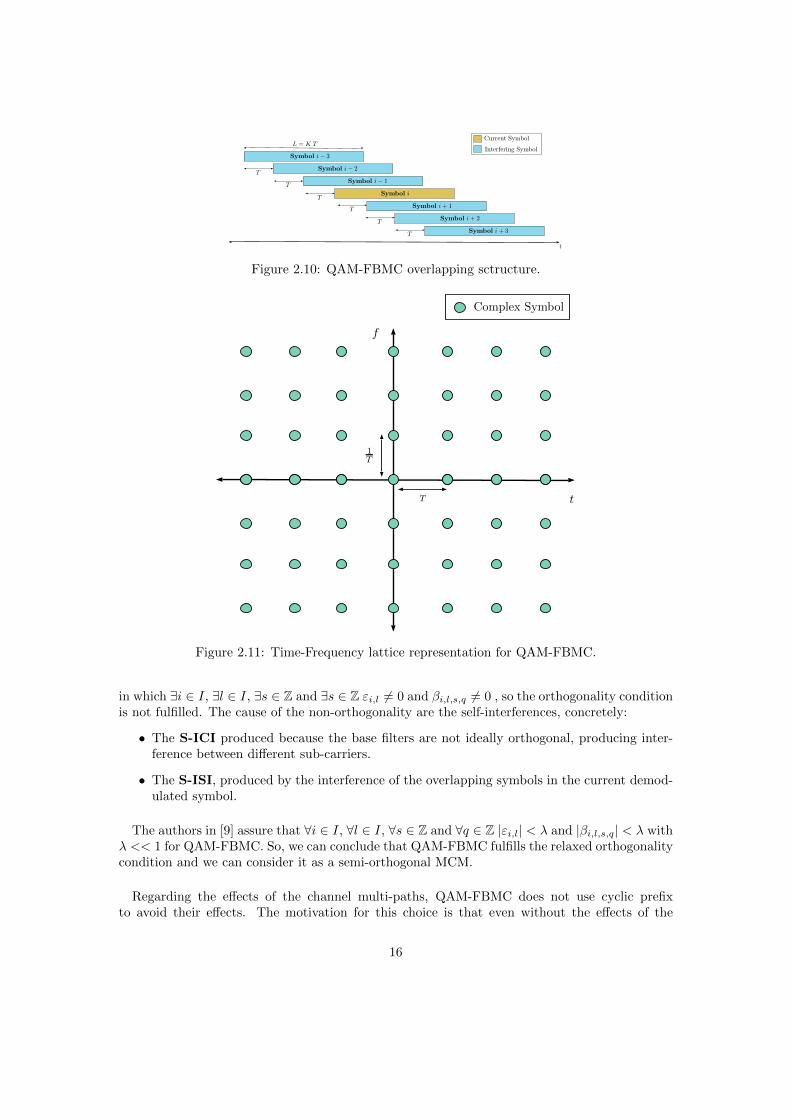
Increasing the length of the filters also produces a not efficient use of the time resources.In order to get an efficient utilization of the time resources using long pulses, QAM-FBMCintroduces overlapping between consecutive symbols. In Figure 2.8 the overlapping operation iscarried out by the block Overlap & Sum. In Figure 2.10 the overlapping structure for QAM-FBMC is shown, where K is the overlapping factor.

In Figure 2.11 the lattice representation for QAM-FBMC has been plotted. The symbol densityis 1, which means that QAM-FBMC offers a very efficient use of the resources. However, as thedensity is equal to 1, OQAM-FBMC is a Non-orthogonal MCM that suffers from S-ICI and S-ISI.

Next, the orthogonality condition is studied for QAM-FBMC. From (2.4)

⟨pi(t− sT ), pl(t− qT )

⟩=

1 if i = l and s = qεi,l if i 6= l and s = q

βi,l,s,q else, (2.10)

15

Symbol i− 3

Symbol i− 2

Symbol i− 1

Symbol i

Symbol i+ 1

Symbol i+ 2

Symbol i+ 3

T

T

T

T

T

T

L = K T

t

Current Symbol

Interfering Symbol

Figure 2.10: QAM-FBMC overlapping sctructure.

f

tT

1T

Complex Symbol

Figure 2.11: Time-Frequency lattice representation for QAM-FBMC.

in which ∃i ∈ I, ∃l ∈ I, ∃s ∈ Z and ∃s ∈ Z εi,l 6= 0 and βi,l,s,q 6= 0 , so the orthogonality conditionis not fulfilled. The cause of the non-orthogonality are the self-interferences, concretely:

• The S-ICI produced because the base filters are not ideally orthogonal, producing inter-ference between different sub-carriers.

• The S-ISI, produced by the interference of the overlapping symbols in the current demod-ulated symbol.

The authors in [9] assure that ∀i ∈ I, ∀l ∈ I, ∀s ∈ Z and ∀q ∈ Z |εi,l| < λ and |βi,l,s,q| < λ withλ << 1 for QAM-FBMC. So, we can conclude that QAM-FBMC fulfills the relaxed orthogonalitycondition and we can consider it as a semi-orthogonal MCM.

Regarding the effects of the channel multi-paths, QAM-FBMC does not use cyclic prefixto avoid their effects. The motivation for this choice is that even without the effects of the

16

channel, QAM-FBMC suffers S-ISI and S-ICI. Adding the CP would improve the robustness ofthe waveform against the ICI and ISI effect produced by the multipaths, but it would worsenthe orthogonality conditions because of the overlap (producing more S-ICI and S-ISI). Thereforeit is reasonable not to use CP. Moreover, not using CP leads to a more efficient use of the timeresources (one of the weakness of OFDM).

In [9] a computationally efficient version of the modulator and demodulator in the digitaldomain can be found, it is based on using the FFT.

To sum up, QAM-FBMC improves the use of the time resources and achieves a lower level ofout-of-band emissions than OFDM. However, it suffers from S-ICI and S-ISI, so perfect recon-struction is not achieved. Studying the robustness of QAM-FBMC against phase noise can behelpful to decide which waveform is more suitable for 5G.

2.1.3 OQAM-FBMC

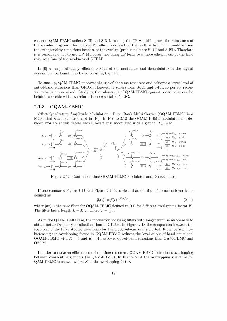
Offset Quadrature Amplitude Modulation - Filter-Bank Multi-Carrier (OQAM-FBMC) is aMCM that was first introduced in [10]. In Figure 2.12 the OQAM-FBMC modulator and de-modulator are shown, where each sub-carrier is modulated with a symbol Xi,s ∈ R.

p(t)

ej2πf0t

t = sT2 ej2πf1t

Overlap

&Sum

⊕

⊗

⊗

⊗

⊗

ej2πfN−2t

ej2πfN−1t

X0,s

X1,s

XN−2,s

XN−1,s

θ0,s⊗

⊗

⊗

⊗

θ1,s

θN−2,s

θN−1,s

e−j2πf0t

e−j2πf1t

⊗

⊗

⊗

⊗

e−j2πfN−2t

e−j2πfN−1t

R0,q q evenθ0⊗

θ1

θN−2

θN−1

⊗

⊗

⊗

ℜ

ℑ

ℜ

ℑ

ℜ

ℑ

ℜ

ℑ

R0,q q odd

R1,q q even

R1,q q odd

RN−2,q q even

RN−2,q q odd

RN−1,q q even

RN−1,q q odd

p(−t)

t = sT2

t = sT2

t = sT2

p(t)

p(t)

p(t)

t = q T2

t = q T2

t = q T2

t = q T2

p(−t)

p(−t)

p(−t)

⊗

fc

⊗

fc

Figure 2.12: Continuous time OQAM-FBMC Modulator and Demodulator.

If one compares Figure 2.12 and Figure 2.2, it is clear that the filter for each sub-carrier isdefined as

pi(t) := p(t) ej2πfit , (2.11)

where p(t) is the base filter for OQAM-FBMC defined in [11] for different overlapping factor K.The filter has a length L = K T , where T = 1

∆f .

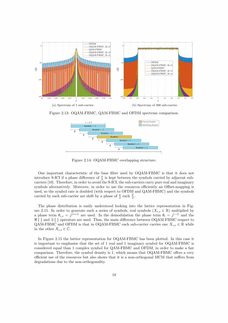
As in the QAM-FBMC case, the motivation for using filters with longer impulse response is toobtain better frequency localization than in OFDM. In Figure 2.13 the comparison between thespectrum of the three studied waveforms for 1 and 300 sub-carriers is plotted. It can be seen howincreasing the overlapping factor in OQAM-FBMC reduces the level of out-of-band emissions.OQAM-FBMC with K = 3 and K = 4 has lower out-of-band emissions than QAM-FBMC andOFDM.

In order to make an efficient use of the time resources, OQAM-FBMC introduces overlappingbetween consecutive symbols (as QAM-FBMC). In Figure 2.14 the overlapping structure forQAM-FBMC is shown, where K is the overlapping factor.

17

-0.1 -0.08 -0.06 -0.04 -0.02 0 0.02 0.04 0.06 0.08 0.1

ν

-150

-100

-50

0

dB

OFDM

OQAM-FBMC, K=2

QAM-FBMC

OQAM-FBMC, K=3

OQAM-FBMC, K=4

(a) Spectrum of 1 sub-carrier.

-0.5 -0.4 -0.3 -0.2 -0.1 0 0.1 0.2 0.3 0.4 0.5

ν

-150

-100

-50

0

dB

OFDM

OQAM-FBMC, K=2

QAM-FBMC

OQAM-FBMC, K=3

OQAM-FBMC, K=4

(b) Spectrum of 300 sub-carrier.

Figure 2.13: OQAM-FBMC, QAM-FBMC and OFDM spectrum comparison.

Symbol i− 3

Symbol i− 2

Symbol i− 1

Symbol i

Symbol i+ 1

Symbol i+ 2

Symbol i+ 3

T2

L = K T

t

Current Symbol

Interfering Symbol

T2

T2

T2

T2

T2

Figure 2.14: OQAM-FBMC overlapping structure.

One important characteristic of the base filter used by OQAM-FBMC is that it does notintroduce S-ICI if a phase difference of π

2 is kept between the symbols carried by adjacent sub-carriers [10]. Therefore, in order to avoid the S-ICI, the sub-carriers carry pure real and imaginarysymbols alternatively. Moreover, in order to use the resources efficiently an Offset-mapping isused, so the symbol rate is doubled (with respect to OFDM and QAM-FBMC) and the symbolscarried by each sub-carrier are shift by a phase of π

2 each T2 .

The phase distribution is easily understood looking into the lattice representation in Fig-ure 2.15. In order to generate such a series of symbols, real symbols (Xi,s ∈ R) multiplied bya phase term θi,s = j(i+s) are used. In the demodulation the phase term θl = j(−l) and the< and = operators are used. Thus, the main difference between OQAM-FBMC respect toQAM-FBMC and OFDM is that in OQAM-FBMC each sub-carrier carries one Xi,s ∈ R whilein the other Xi,s ∈ C.

In Figure 2.15 the lattice representation for OQAM-FBMC has been plotted. In this case itis important to emphasise that the set of 1 real and 1 imaginary symbol for OQAM-FBMC isconsidered equal than 1 complex symbol for QAM-FBMC and OFDM, in order to make a faircomparison. Therefore, the symbol density is 1, which means that OQAM-FBMC offers a veryefficient use of the resources but also shows that it is a non-orthogonal MCM that suffers fromdegradations due to the non-orthogonality.

18

f

tT2

1T

Imaginary Symbol

Real Symbol

Figure 2.15: Time-Frequency lattice representation for OQAM-FBMC.

Next, the orthogonality condition is studied for OQAM-FBMC. Due to the use of the Offset-mapping, the orthogonality condition in (2.4) has to be modified including the phase terms andthe < operator, giving 3

<⟨

θi,s pi

(t− sT

2

), θl pl

(t− T

2

)⟩=

1 if i = l and s = qεi,l if i 6= l and s = q

βi,l,s,q else, (2.12)

in which εi,l and βi,ls,q are related with the S-ICI and S-ISI degradations respectively. As hasbeen studied previously, OQAM-FBMC is not affected by S-ICI if the phase difference betweenneighbour sub-carriers is π

2 , so ∀i ∈ I and ∀l ∈ I εi,l = 0. However, due to the overlap betweenconsecutive symbols it is affected by S-ISI effect, so ∃i ∈ I, ∃l ∈ I, ∃s ∈ Z and ∃s ∈ Z βi,l,s,q 6= 0.Thus the orthogonality condition is not fulfilled because of the S-ISI effect.

The authors in [11] assure that ∀i ∈ I, ∀l ∈ I, ∀s ∈ Z and ∀q ∈ Z |βi,l,s,q| < λ with λ << 1 .Therefore, we can conclude that OQAM-FBMC fulfills the relaxed orthogonality condition andwe can consider it as a semi-orthogonal MCM.

Regarding the effects of the multipaths in the channel, OQAM-FBMC does not use cyclicprefix to avoid them. The motivation is the same than for the case of QAM-FBMC.

3The expression in (2.12) is only valid for even l. For odd l the = operator would replace the < operator.

19

One of the weakness of OQAM-FBMC compared to (OFDM and QAM-FBMC) is its perfor-mance in complex channels. When the channel has complex coefficients the phase difference ofπ2 between neighbour sub-carriers could be modified, producing the appearance of S-ICI.

In [10] a computationally efficient version of the modulator and demodulator in the digitaldomain can be found, it is based in the use of the FFT and poly-phase networks.

To sum up, OQAM-FBMC improves the use of the time resources respect to OFDM andachieves lower level of out-of-band emissions than OFDM (but higher than QAM-FBMC). More-over, for real channels it is not affected by S-ICI, so it suffers less degradations than QAM-FBMCbut more than OFDM. However, for complex channels it suffers from severe S-ICI.

2.2 Phase noise

Oscillators are important elements of transmitters and receivers in wireless systems. The mainfunction of oscillators is to up-convert a base-band signal to a radio-frequency signal at the trans-mitter and down-convert a radio-frequency signal to a base-band signal at the receiver. Ideally,an oscillator generates a perfect sinusoidal signal with frequency fo. In practical situations, thesignal generated by oscillators is not perfect and has low random fluctuations in the phase, whichare usually called phase noise. An oscillator with a central frequency fo and the effects of phasenoise can be modelled as

V (t) = ej(2πtfo+φ(t)) ,

in which φ(t) is an stochastic process that modifies the phase of the ideal sinusoidal signal, calledphase noise.

The main effect of phase noise in the oscillator output signal is an spreading on its PowerSpectral Density (PSD), which ideally is a Dirac Delta in the central frequency fo. This effectcan be seen in Figure 2.16.

ffo

PSD

(a) Ideal oscillator

ffo

PSD

(b) Real oscillator

Figure 2.16: Spreading produced by phase noise in the PSD of the oscillator.

The specific properties of phase noise depend on each particular oscillator. There are severaltypes of oscillator, but the most used ones for Wireless systems are the ones using a Phase-Locked Loop Synthesizer (PLL). In Figure 2.17 the main structure of an oscillator based on PLLis shown. In this model, the phase of the Voltage Controlled Oscillator (VCO) is compared witha reference signal produced by a Free-Running Oscillator (Reference oscillator), the differencebetween both phases is filtered using a low pass-filter (LPF) and applied as a control signal to the

20

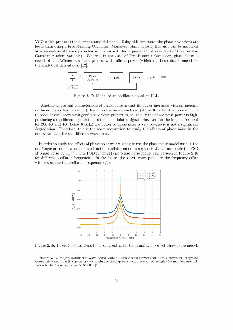
VCO which produces the output sinusoidal signal. Using this structure, the phase deviations arelower than using a Free-Running Oscillator. Moreover, phase noise in this case can be modelledas a wide-sense stationary stochastic process with finite power and φ(t) ∼ N (0, σ2) (zero-meanGaussian random variable). Whereas in the case of Free-Running Oscillator, phase noise ismodelled as a Wiener stochastic process with infinite power (which is a less suitable model forthe analytical derivations) [12].

Phasedetector

LPF VCO ej(2πtfo+φ(t))

ReferenceOscillator

fR

Figure 2.17: Model of an oscillator based on PLL.

Another important characteristic of phase noise is that its power increases with an increasein the oscillator frequency (fo). For fo in the mm-wave band (above 30 GHz) it is more difficultto produce oscillators with good phase noise properties, so usually the phase noise power is high,producing a significant degradation in the demodulated signal. However, for the frequencies usedfor 2G, 3G and 4G (below 6 GHz) the power of phase noise is very low, so it is not a significantdegradation. Therefore, this is the main motivation to study the effects of phase noise in themm-wave band for the different waveforms.

In order to study the effects of phase noise we are going to use the phase noise model used in themmMagic project 4, which is based on the oscillator model using the PLL. Let us denote the PSDof phase noise by Sφ(f). The PSD for mmMagic phase noise model can be seen in Figure 2.18for different oscillator frequencies. In the figure, the x-axis corresponds to the frequency offsetwith respect to the oscillator frequency (fo).

-50 -40 -30 -20 -10 0 10 20 30 40 50

Frequency Offset [MHz]

-160

-140

-120

-100

-80

-60

-40

Sφ(f

)[dBW

]

fo = 82 GHzfo = 28 GHzfo = 6 GHz

Figure 2.18: Power Spectral Density for different fo for the mmMagic project phase noise model.

4mmMAGIC project (Millimetre-Wave Based Mobile Radio Access Network for Fifth Generation IntegratedCommunications) is a European project aiming to develop novel radio access technologies for mobile communi-cation in the frequency range 6-100 GHz [13]

21

2.2.1 Effect of phase noise in a generic signal

Let us consider x(t) as the base-band modulated signal. In the transmitter, the base-bandsignal is up-converted to a radio-frequency signal using an oscillator with frequency fc

xc(t) = x(t) ej(2πfct+φt(t)) , (2.13)

where φt(t) is the phase noise impulse response for the transmitter oscillator.

In the receiver, the received radio-frequency signal is given by

rc(t) = xc(t) ∗ h(t) + w(t) ,

where ∗ denotes convolution operation, h(t) is the impulse response of the radio-channel andw(t) is AWGN noise.

Although in a real transmission the effects of the channel can not be disregarded, in all thefollowing derivations an ideal flat channel with non additive noise will be assumed, i.e., h(t) = δ(t)and w(t) = 0 for any t. Taking this assumption, the previous expression can be modified as

rc(t) = xc(t) (2.14)

The motivation for this assumption is to study the effects only produced by phase noise.

Next, the received radio-frequency signal is down-converted in order to get base band signal

r(t) = rc(t) e−(j2πfc+φr(t)) (a)= xc(t) e−(j2πfc+φr(t)) (b)

= x(t) ej(φt(t)−φr(t)) , (2.15)

where φr(t) is the phase noise introduced by receiver’s oscillator; (a) follows from (2.14); (b)follows from (2.13).

A random variable with the effect of phase noise of both oscillators is included in (2.14),resulting in the following expression

r(t) = x(t) ejφ(t) , (2.16)

in which φ(t) = φt(t)− φr(t).

As φ(t) ∼ N (0, σ2) with very small σ2 and sin(x) ≈ x if |x| 1, we are going to use thefollowing approximation

ejφ(t) ≈ 1 + jφ(t) (2.17)

This approximation has been widely used in the literature [3] [4] and simplifies significantly theanalysis of the effect of phase noise in the different waveforms. Finally, the expression for thereceived base-band signal with the effects of phase noise is given by

r(t) ≈ x(t) (1 + jφ(t)) (2.18)

22

Chapter 3

OFDM

Orthogonal Frequency Division Multiplexing (OFDM) is an orthogonal MCM widelyused in wireless systems (for example IEEE 802.11g/n/ac and LTE) as discussed in Section 2.1.1.An important feature of a waveform for 5G is its robustness against phase noise (as was explainedin Chapter 1). So, this chapter presents the derivations and evaluations carried out in order tostudy the effects of phase noise in OFDM. Concretely, the effects of phase noise are studied for thecontinuous and discrete time OFDM with the objective of showing the effects of sampling. So, forboth cases, we start deriving the expressions for the modulated and demodulated signals. Nextwe study the effect of phase noise in the demodulated signal, deriving expressions for the powerof interference terms produced by phase noise. In the following we derive the expressions for theSymbol-to-Interference Ratio (SIR). Once the expression for the SIR for both cases (continuousand discrete) are obtained, an analysis of the functions that determine the value of the SIR iscarried out (we refer to these functions as weighting functions). Next, a comparison between thecontinuous and discrete time is done. Finally, the SIR and SER are evaluated for some concreteimplementation parameters.

3.1 Continuous time Modulated and Demodulated signal

Modulated signal The continuous time base-band modulated signal for an OFDM symbol isgiven by

x(t) =∑

i∈IXi p(t) ej2π

iT t =

∑

i∈IXi pi(t) , (3.1)

where Xi is any mapped symbol that modulates sub-carrier i, I is the set of indices for the activesub-carriers, T is the length of the OFDM symbol (without the contribution of the CP), p(t) isthe base filter defined in (2.6) and pi(t) is the filter for sub-carrier i defined in (2.8).

Demodulated signal In Section 2.1 the demodulation using matched filter was presented, itis the most common demodulation procedure for MCM. OFDM uses the matched filter demod-ulation, so the demodulated symbol in sub-carrier l follows from (2.2) and it is given by

Rl = r(t) ∗ gl(t)∣∣∣∣t=0

, (3.2)

where gl(t) is the matched filter used in sub-carrier l. It is defined as

gl(t) := pl(−t) (3.3)

23

3.2 Continuous time Demodulated signal subject to phasenoise

Once the expressions for the modulated and demodulated signal are known, we are going tostudy the effects of phase noise in the demodulated signal.

The demodulated signal subject to phase noise is given by

Rl(a)= r(t) ∗ gl(t)

∣∣∣∣t=0

(b)=[x(t)

(1 + jφ(t)

)]∗ gl(t)

∣∣∣∣t=0

(c)=

[∑

i∈IXi pi(t)

(1 + jφ(t)

)]∗ gl(t)

∣∣∣∣t=0

(d)=∑

i∈IXi

[pi(t) ∗ gl(t)

∣∣∣∣t=0

]+∑

i∈IXi

[jφ(t) pi(t) ∗ gl(t)

∣∣∣∣t=0

]

(e)=∑

i∈IXiλi,l +

∑

i∈IXiϕi,l (3.4)

(a) follows from the definition of the demodulated signal in (3.2) while ∗ is the convolutionoperator; (b) follows from the effect of phase noise in the received signal in (2.18); (c) followsfrom (3.1); (d) follows from the distributivity property of the convolution; (e) follows by defining

λi,l := pi(t) ∗ gl(t)∣∣t=0

and ϕi,l :=[jφ(t)pi(t)

]∗ gl(t)

∣∣t=0

.

The terms in (3.4) that only depend on the impulse response of the transmitter and receiverfilter are

λi,l = pi(t) ∗ gl(t)∣∣∣∣t=0

(a)= 〈pi(t), pl(t)〉

(b)= δi,l (3.5)

(a) follows from the convolution definition in t = 0 and from (3.3); (b) follows from the orthogo-nality condition for OFDM in (2.7). This is a very important result, because it means that whenthe orthogonality condition is fulfilled there are no self-interferences in the demodulation.

The terms in (3.4) that do not only depend on the impulse response of the transmitter andreceiver filter but also on the phase noise are

ϕi,l =[jφ(t) pi(t)

]∗ gl(t)

∣∣∣∣t=0

(a)=

∫ ∞

−∞jφ(τ)pi(τ) gl(−τ) dτ

(b)=

∫ ∞

−∞jφ(τ)pi(τ) pl(τ) dτ (3.6)

(a) follows from the convolution definition in t = 0; (b) follows from (3.3). These terms arerelated with the interference terms produced by phase noise.

Taking into consideration the previous definitions in (3.5) and (3.6), we can rewrite (3.4) as

Rl = Xl + NCPEl + N ICI

l , (3.7)

24

where NCPEl and N ICI

l are two interference terms produced by phase noise. They are definedas

NCPEl := Xl ϕl,l (3.8)

N ICIl :=

∑

i∈IICIXi ϕi,l (3.9)

where IICI is the set of indices for the interfering sub-carriers. It is defined as IICI = I\l.

As shown in (3.7), phase noise introduces two interference terms in the demodulated signal.We are going to classify these interferences as:

• Phase noise - Common Phase Error (PN-CPE). It is identified with the term NCPEl

and it is a rotated version of the ideally transmitted symbol Xl. The rotation is given bythe term ϕl,l, which is equal for every sub-carrier l. This fact makes the PN-CPE correctiona very easy process using pilot symbols.

• PN - Inter-Carrier Interference (PN-ICI). The introduction of phase noise worsensthe orthogonality between sub-carriers, so interference from the rest of the sub-carriersappears in the demodulated sub-carrier, producing the interference term N ICI

l .

3.2.1 Interference power

In this section the power of the interference terms NCPEl and N ICI

l produced by phase noiseare derived.

The power of the interference terms is given by

PNCPEl:= E

[|Xlϕl,l|2

]= E

[|Xl|2

]E[|ϕl,l|2

]= EX

(E[|ϕl,l|2

])(3.10)

PNICIl:= E

∣∣∣∣∣∑

i∈IICIXiϕi,l

∣∣∣∣∣

2 =

∑

i∈IICIE[|Xi|2

]E[|ϕi,l|2

]= EX

( ∑

i∈IICIE[|ϕi,l|2

])(3.11)

In (3.10) and (3.11) it has been assumed that Xi ∀i ∈ I is a sequence of zero-mean independentrandom variables and ϕi,l is a sequence of random variables whose elements are independentfrom the elements of Xi ∀i ∈ I and ∀l ∈ I. Moreover, EX is the power of the mapped symbol

and it is defined as EX = E[|Xl|2

]∀l ∈ I.

The expression for the power of the interference terms in (3.10) and (3.11) is dependent on

the term E[|ϕi,l|2

]. According to Appendix A.1, E

[|ϕi,l|2

], can be expressed as

E[|ϕi,l|2

]=

∫ +∞

−∞Sφ(f) Wi,l(f) df , (3.12)

where Sφ(f) is the PSD of phase noise and Wi,l(f) is defined as

Wi,l(f) :=

∣∣∣∣sinc

((f − i− l

T

)T

)∣∣∣∣2

(3.13)

25

Applying the previous result in (3.12) to (3.10) and (3.11) the final expressions for the powerof the interference terms is obtained as

PNCPEl= EX

(∫ ∞

−∞WCPEl (f) Sφ(f)df

)(3.14)

PNICIl= EX

(∫ ∞

−∞W ICIl (f) Sφ(f)df

)(3.15)

in which

WCPEl (f) : = Wl,l(f) (3.16)

W ICIl (f) : =

∑

i∈IICIWi,l(f) (3.17)

3.2.2 Signal-to-Interference Ratio due to phase noise

From (3.7) the expression for the SIR in the demodulated signal in sub-carrier l subject tophase noise is easily derived, giving

SIRl =EX

PNCPEl+ PNICIl

(a)=

1∫∞−∞

[WCPEl (f) + W ICI

l (f)]Sφ (f) df

(3.18)

(a) follows from (3.14) and (3.15). Moreover, PNCPEland PNICIl

are the power of the interferenceterms produced by the PN-CPE and PN-ICI respectively and EX is the power of the transmitted

symbol in the active sub-carrier l, and it is defined as EX := E[|Xl|2

].

Effect of removing PN-CPE The expression for the SIR without the effect of PN-CPE insub-carrier l is easily derived from (3.18) by removing the CPE contribution, giving

SIRl =1∫∞

−∞ W ICIl (f)Sφ (f) df

(3.19)

3.3 Discrete time Modulated and Demodulated signal

Modulated signal The discrete time modulated signal for an OFDM symbol is given by

x[n] =

√T

Nx(t)

∣∣∣t= n

fs

=∑

i∈IXi p[n]ej2π

iN n =

∑

i∈IXi pi[n] , (3.20)

where N is the total number of samples of one OFDM symbol (without the CP length), Xi isthe modulated symbol in sub-carrier i, I is the set with the index of active sub-carriers, fs isthe samlping frequency, p[n] is the discrete time base filter, pi[n] is the discrete time filter for

sub-carrier i and√

TN is a scaling term whose goal is to have the same total energy for x[n] as

for x(t).

The base filter for the discrete time implementation can be considered as a sampled and scaledversion of the filter in (2.6), defined as

p[n] :=

√T

Np(t)

∣∣∣t= n

fs

=

1√N

if 0 ≤ n ≤ N − 1

0 else(3.21)

The scaling is motivated by having a filter with a total energy equal to 1, i.e.,∑+∞n=−∞ |p[n]|2 = 1.

26

The filter for sub-carrier i for the discrete time implementation is a shifted version of the basefilter in (3.21), given by

pi[n] := p[n] ej2πiN n (3.22)

Demodulated signal As in the continuous time case, the demodulation in the discrete timecase is performed using the matching filter demodulation. Therefore, the demodulated signal insub-carrier l follows from (2.2) and it is given by

Rl = r[n] ∗ gl[n]

∣∣∣∣n=0

, (3.23)

where r[n] is the sampled base-band received signal, ∗ is the convolution operator and gl[n] isthe matched filter for sub-carrier l, which is defined as

gl[n] := pl[−n] (3.24)

3.4 Discrete time Demodulated signal subject to phasenoise

In this section we study the effect that has the sampling of the continuous signal and thefollowing discrete time demodulation in the degradations produced by phase noise.

The sampled base-band received signal with a sample rate fs subject to phase noise is givenby

r[n] =

√T

Nr(t)

∣∣∣∣t= n

fs

(a)=

√T

Nx(t) (1 + jφ(t))

∣∣∣∣t= n

fs

(b)= x[n] (1 + jφ[n]) (3.25)

(a) follows from the definition of the received signal with the effects of phase noise in (2.18); (b)

follows from (3.20) and from the sampled version of φ(t), which is

φ[n] = φ(t)

∣∣∣∣t= n

fs

(3.26)

The demodulated signal subject to phase noise using a discrete time demodulator is given by

Rl(a)= r[n] ∗ gl[n]

∣∣∣∣n=0

(b)= Xl +NCPE

l +N ICIl (3.27)

(a) follows from the definition of the demodulated signal for the discrete time implementationin (3.23); (b) follows from the same procedure as in (3.4) and (3.7) but replacing the continuoussignals by the sampled ones. Therefore, the noise terms for the discrete case are defined as

NCPEl := Xl ϕl,l (3.28)

N ICIl :=

∑

i∈IICIXi ϕi,l (3.29)

27

In the previous expressions (3.28) and (3.29), ϕi,l is a random variable that contains the phasenoise terms for the discrete case. Similarly to the case of ϕi,l in (3.6), ϕi,l is defined as

ϕi,l :=(jφ[n] pi[n]

)∗ gl[n]

∣∣∣∣n=0

=

∞∑

s=−∞jφ[s] pi[s] pl[s] , (3.30)

where we have the same derivation as in (3.6) replacing the continuous signals by its sampledversion.

From the previous results in (3.28) and (3.29) we can conclude that the two different kindof interferences produced in the discrete time case are the same than in the continuous timecase, i.e., the interference types are PN-CPE and PN-ICI. In the following sections we study thedifferences on the power of this interferences between the discrete and continuous time cases.

It is important to say that in the sampling no anti-aliasing filter has been used. The motivationfor this decision is that for frequencies outside the sampling bandwidth neither the signal nor thephase noise have significant components, so the aliasing introduced by the sampling is negligible.Not considering the anti-aliasing filter gives a more suitable set of equations.

3.4.1 Interference power

In this section the power of the interference terms NCPEl and N ICI

l is derived. The derivationfollows the same steps than (3.10) and (3.11). Therefore, the power of the noise terms is givenby

PNCPEl:= EX

(E[|ϕl,l|2

])(3.31)

PNICIl:= EX

( ∑

i∈IICIE[|ϕi,l|2

])(3.32)

According to Appendix A.2, E [ϕi,l] is given by

E [ϕi,l] =

∫ +0.5

−0.5

Sφ(ν)Wi,l(ν) dν , (3.33)

in which ν is the normalized frequency (ν := ffs

), Sφ(ν) := fs∑∞k=−∞ Sφ((ν − k) fs) is the PSD

of the sampled phase noise and Wi,l(ν) is defined as

Wi,l(ν) :=1

N2

∣∣∣∣∣∣

sin(π(ν − i−l

N

)N)

sin(π(ν − i−l

N

) )

∣∣∣∣∣∣

2

(3.34)

Applying the previous result in (3.33) to (3.31) and (3.32) the final expressions for the powerof the interference terms is obtained

PNCPEl= EX

(∫ +0.5

−0.5

Sφ(ν)WCPEl (ν) dν

)(3.35)

PNICIl= EX

(∫ +0.5

−0.5

Sφ(ν)W ICIl (ν) dν

)(3.36)

28

where

WCPEl (ν) : = Wl,l(ν) (3.37)

W ICIl (ν) : =

∑

i∈IICIWi,l(ν) (3.38)

3.4.2 Signal-to-Interference Ratio due to phase noise

From (3.27) the expression for the SIR in the demodulated signal in sub-carrier l subject tophase noise is easily derived, obtaining

SIRl =EX

PNCPEl+ PNICIl

(a)=

1∫ +0.5

−0.5

[WCPEl (ν) +W ICI

l (ν)]Sφ (ν) dν

(3.39)

(a) follows from (3.35) and (3.36). PNCPEland PNICIl

are the power of the interference termsproduced by the PN-CPE and PN-ICI respectively and EX is the power of the transmitted

symbol in the active sub-carrier l, and it is defined as EX := E[|Xl|2

].

Effect of removing PN-CPE The expression for the SIR without the effect of PN-CPE insub-carrier l is easily derived from (3.39) by removing the PN-CPE contribution, giving

SIRl =EXPNICIl

=1∫ +0.5

−0.5W ICIl (ν)Sφ (ν) dν

(3.40)

3.5 Weighting functions

In this section we present the tools usually used in MCM to compute the power of the inter-ferences caused by phase noise. In general, in the literature these tools are known as weightingfunctions. Previously they were used in [3].

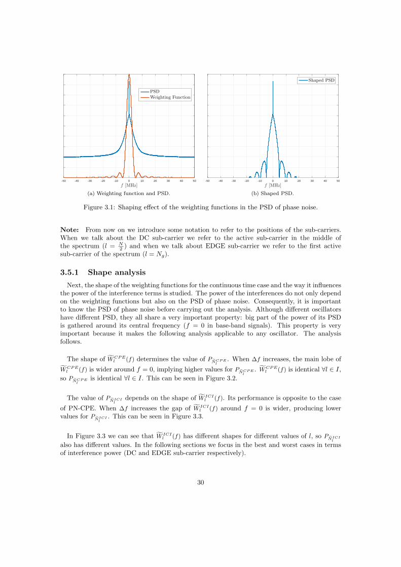
Weighting functions provide a graphical understanding of the level of the interferences pro-duced by phase noise. They shape its PSD in order to get the total power of the interferences,i.e., they indicate for which frequencies the PSD of phase noise has less and more influence in thetotal power of the interference terms. This effect can be seen in Figure 3.1. Thus, if the shapeof the weighting functions and the PSD of phase noise are known, it can be understood how thepower of the interference terms changes as a function of different parameters of the waveforms(as ∆f).

In Section 3.2.1 we derived the expressions for the power of the interferences produced byphase noise for continuous time OFDM. The final expressions were

PNCPEl= EX

(∫ ∞

−∞WCPEl (f) Sφ(f)df

)

PNICIl= EX

(∫ ∞

−∞W ICIl (f) Sφ(f)df

)

In the previous expression Sφ(f) is multiplied by some functions that change its shape. This

functions are WCPEl (f) and W ICI

l (f), which we are going to call weighting functions for thePN-CPE and PN-ICI effects respectively. They were previously defined in (3.16) and (3.17).

29

-50 -40 -30 -20 -10 0 10 20 30 40 50

f [MHz]

PSDWeighting Function

(a) Weighting function and PSD.

-50 -40 -30 -20 -10 0 10 20 30 40 50

f [MHz]

Shaped PSD

(b) Shaped PSD.

Figure 3.1: Shaping effect of the weighting functions in the PSD of phase noise.

Note: From now on we introduce some notation to refer to the positions of the sub-carriers.When we talk about the DC sub-carrier we refer to the active sub-carrier in the middle ofthe spectrum (l = N

2 ) and when we talk about EDGE sub-carrier we refer to the first activesub-carrier of the spectrum (l = Ng).

3.5.1 Shape analysis

Next, the shape of the weighting functions for the continuous time case and the way it influencesthe power of the interference terms is studied. The power of the interferences do not only dependon the weighting functions but also on the PSD of phase noise. Consequently, it is importantto know the PSD of phase noise before carrying out the analysis. Although different oscillatorshave different PSD, they all share a very important property: big part of the power of its PSDis gathered around its central frequency (f = 0 in base-band signals). This property is veryimportant because it makes the following analysis applicable to any oscillator. The analysisfollows.

The shape of WCPEl (f) determines the value of PNCPE

l. When ∆f increases, the main lobe of

WCPEl (f) is wider around f = 0, implying higher values for PNCPE

l. WCPE

l (f) is identical ∀l ∈ I,

so PNCPEl

is identical ∀l ∈ I. This can be seen in Figure 3.2.

The value of PNICIl

depends on the shape of W ICIl (f). Its performance is opposite to the case

of PN-CPE. When ∆f increases the gap of W ICIl (f) around f = 0 is wider, producing lower

values for PNICIl

. This can be seen in Figure 3.3.

In Figure 3.3 we can see that W ICIl (f) has different shapes for different values of l, so PNICI

l

also has different values. In the following sections we focus in the best and worst cases in termsof interference power (DC and EDGE sub-carrier respectively).

30

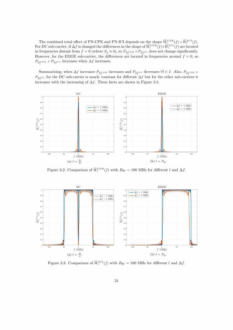
The combined total effect of PN-CPE and PN-ICI depends on the shape WCPEl (f) + W ICI

l (f).For DC sub-carrier, if ∆f is changed the differences in the shape of WCPE

l (f)+W ICIl (f) are located

in frequencies distant from f = 0 (where Sφ ≈ 0), so PNCPEl

+PNICIl

does not change significantly.

However, for the EDGE sub-carrier, the differences are located in frequencies around f = 0, soPNCPE

l+ PNICI

lincreases when ∆f increases.

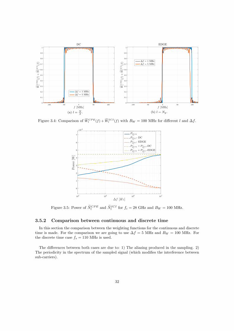
Summarizing, when ∆f increases PNCPEl

increases and PNICIl

decreases ∀l ∈ I. Also, PNCPEl

+

PNICIl

for the DC sub-carrier is nearly constant for different ∆f but for the other sub-carriers it

increases with the increasing of ∆f . These facts are shown in Figure 3.5.

-100 -50 0 50 100

f [MHz]

0

0.1

0.2

0.3

0.4

0.5

0.6

0.7

0.8

0.9

1

WCPE

l(f)

DC

∆f = 1 MHz∆f = 5 MHz

(a) l = N2

.

-100 -50 0 50 100

f [MHz]

0

0.1

0.2

0.3

0.4

0.5

0.6

0.7

0.8

0.9

1

WCPE

l(f)

EDGE

∆f = 1 MHz∆f = 5 MHz

(b) l = Ng .

Figure 3.2: Comparison of WCPEl (f) with BW = 100 MHz for different l and ∆f .

-100 -50 0 50 100

f [MHz]

0

0.1

0.2

0.3

0.4

0.5

0.6

0.7

0.8

0.9

1

WICI

l(f)

DC

∆f = 1 MHz∆f = 5 MHz

(a) l = N2

.

-100 -50 0 50 100

f [MHz]

0

0.1

0.2

0.3

0.4

0.5

0.6

0.7

0.8

0.9

1

WICI

l(f)

EDGE

∆f = 1 MHz∆f = 5 MHz

(b) l = Ng .

Figure 3.3: Comparison of W ICIl (f) with BW = 100 MHz for different l and ∆f .

31

-100 -50 0 50 100

f [MHz]

0

0.1

0.2

0.3

0.4

0.5

0.6

0.7

0.8

0.9

1

WCPE

l(f)+

WICI

l(f)

DC

∆f = 1 MHz∆f = 5 MHz

(a) l = N2

.

-100 -50 0 50 100

f [MHz]

0

0.1

0.2

0.3

0.4

0.5

0.6

0.7

0.8

0.9

1

WCPE

l(f)+

WICI

l(f)

EDGE

∆f = 1 MHz∆f = 5 MHz

(b) l = Ng .

Figure 3.4: Comparison of WCPEl (f) + W ICI

l (f) with BW = 100 MHz for different l and ∆f .

104 105 106 107

∆f [Hz]

0

1

2

3

4

5

6

7

Pow

er[W

]

×10-4

PNCPE

l

PN ICI

l

- DC

PN ICI

l

- EDGE

PNCPE

l

+ PN ICI

l

-DC

PNCPE

l

+ PN ICI

l

-EDGE

Figure 3.5: Power of NCPEl and N ICI

l for fc = 28 GHz and BW = 100 MHz.

3.5.2 Comparison between continuous and discrete time

In this section the comparison between the weighting functions for the continuous and discretetime is made. For the comparison we are going to use ∆f = 5 MHz and BW = 100 MHz. Forthe discrete time case fs = 110 MHz is used.

The differences between both cases are due to: 1) The aliasing produced in the sampling. 2)The periodicity in the spectrum of the sampled signal (which modifies the interference betweensub-carriers).

32

In Figure 3.6, WCPEl and WCPE

l have been plotted. The differences in the shape of bothweighting functions are insignificant. Taking into consideration that Sφ(f) ≈ 0 for |f | > fs

2 , wecan state that PNCPE

l≈ PNCPE

l∀l ∈ I.

-50 -40 -30 -20 -10 0 10 20 30 40 50

f [MHz]

0

0.1

0.2

0.3

0.4

0.5

0.6

0.7

0.8

0.9

1

WCPE

l(f)

(a) Continuous time.

-0.5 -0.4 -0.3 -0.2 -0.1 0 0.1 0.2 0.3 0.4 0.5

ν

0

0.1

0.2

0.3

0.4

0.5

0.6

0.7

0.8

0.9

1

WCPE

l(ν)

(b) Discrete time.

Figure 3.6: Comparison of WCPEl and WCPE

l .

In Figure 3.7 we have plotted W ICIl and W ICI

l for the DC sub-carrier. As in the case of PN-CPE, the differences in the shape of W ICI

l and W ICIl are negligible. Taking into consideration

that Sφ(f) ≈ 0 for |f | > fs2 , we can consider PNICI

l≈ PNICI

lfor the DC sub-carrier.

-50 -40 -30 -20 -10 0 10 20 30 40 50

f [MHz]

0

0.1

0.2

0.3

0.4

0.5

0.6

0.7

0.8

0.9

1

WICI

l(f)

DC

(a) Continuous time.

-0.5 -0.4 -0.3 -0.2 -0.1 0 0.1 0.2 0.3 0.4 0.5

ν

0

0.1

0.2

0.3

0.4

0.5

0.6

0.7

0.8

0.9

1

WICI

l(ν)

DC

(b) Discrete time.

Figure 3.7: Comparison of W ICIl and W ICI

l in the DC sub-carrier.

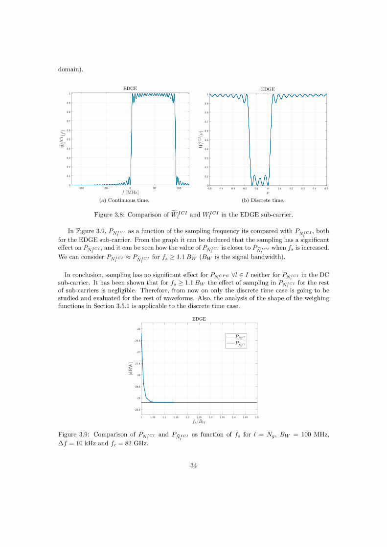
In Figure 3.8, W ICIl and W ICI

l for the EDGE sub-carrier have been plotted. This case isthe one in which the differences between the shapes of W ICI

l and W ICIl are higher and more

noticeable. Therefore, for the EDGE sub-carrier it is important to study the differences betweenPNICIl

and PNICIl(which are produced by the periodicity of the sampled signal in the frequency

33

domain).

-100 -50 0 50 100

f [MHz]

0

0.1

0.2

0.3

0.4

0.5

0.6

0.7

0.8

0.9

1

WICI

l(f)

EDGE

(a) Continuous time.

-0.5 -0.4 -0.3 -0.2 -0.1 0 0.1 0.2 0.3 0.4 0.5

ν

0

0.1

0.2

0.3

0.4

0.5

0.6

0.7

0.8

0.9

1

WICI

l(ν)

EDGE

(b) Discrete time.

Figure 3.8: Comparison of W ICIl and W ICI

l in the EDGE sub-carrier.

In Figure 3.9, PNICIlas a function of the sampling frequency its compared with PNICIl

, both

for the EDGE sub-carrier. From the graph it can be deduced that the sampling has a significanteffect on PNICIl

, and it can be seen how the value of PNICIlis closer to PNICIl

when fs is increased.

We can consider PNICIl≈ PNICIl

for fs ≥ 1.1BW (BW is the signal bandwidth).

In conclusion, sampling has no significant effect for PNCPEl∀l ∈ I neither for PNICIl

in the DCsub-carrier. It has been shown that for fs ≥ 1.1BW the effect of sampling in PNICIl

for the restof sub-carriers is negligible. Therefore, from now on only the discrete time case is going to bestudied and evaluated for the rest of waveforms. Also, the analysis of the shape of the weighingfunctions in Section 3.5.1 is applicable to the discrete time case.

1 1.05 1.1 1.15 1.2 1.25 1.3 1.35 1.4 1.45 1.5

fs/BW

-29.5

-29

-28.5

-28

-27.5

-27

-26.5

-26

[dBW

]

EDGE

PN ICIl

PN ICI

l

Figure 3.9: Comparison of PNICIland PNICIl

as function of fs for l = Ng, BW = 100 MHz,

∆f = 10 kHz and fc = 82 GHz.

34

3.6 Signal-to-Interference Ratio evaluations

In this section we evaluate the SIR using the derived expressions, also using simulations. Theparameters BW = 100 MHz and fs = 110 MHz have been used.

3.6.1 Theoretical results

The theoretical evaluations for the Signal-to-Interference Ratio produced by phase noise arepresented in this section. The results have been obtained with the expressions derived in Sec-tion 3.4.2 and taking as phase noise model the mmMagic project phase noise model introducedin Section 2.2.

SIR due to phase noise In Figure 3.10 the SIR as a function of ∆f including the effectsof PN-CPE and PN-ICI has been plotted (for the EDGE and DC sub-carrier). In the graphit is obvious that degradations produced by phase noise are more important for high carrierfrequencies. Also, the SIR does not change much in relation with ∆f .

101 102 103

∆f [kHz]

20

25

30

35

40

45

50

55

60

SIR

l[dB]

fc = 82 GHz - DCfc = 82 GHz - EDGEfc = 28 GHz - DCfc = 28 GHz - EDGEfc = 6 GHz - DCfc = 6 GHz - EDGE

Figure 3.10: SIR due to phase noise (including PN-CPE and PN-ICI effects) for three differentfc and two different values of l, with BW = 100 MHz and fs = 110 MHz.

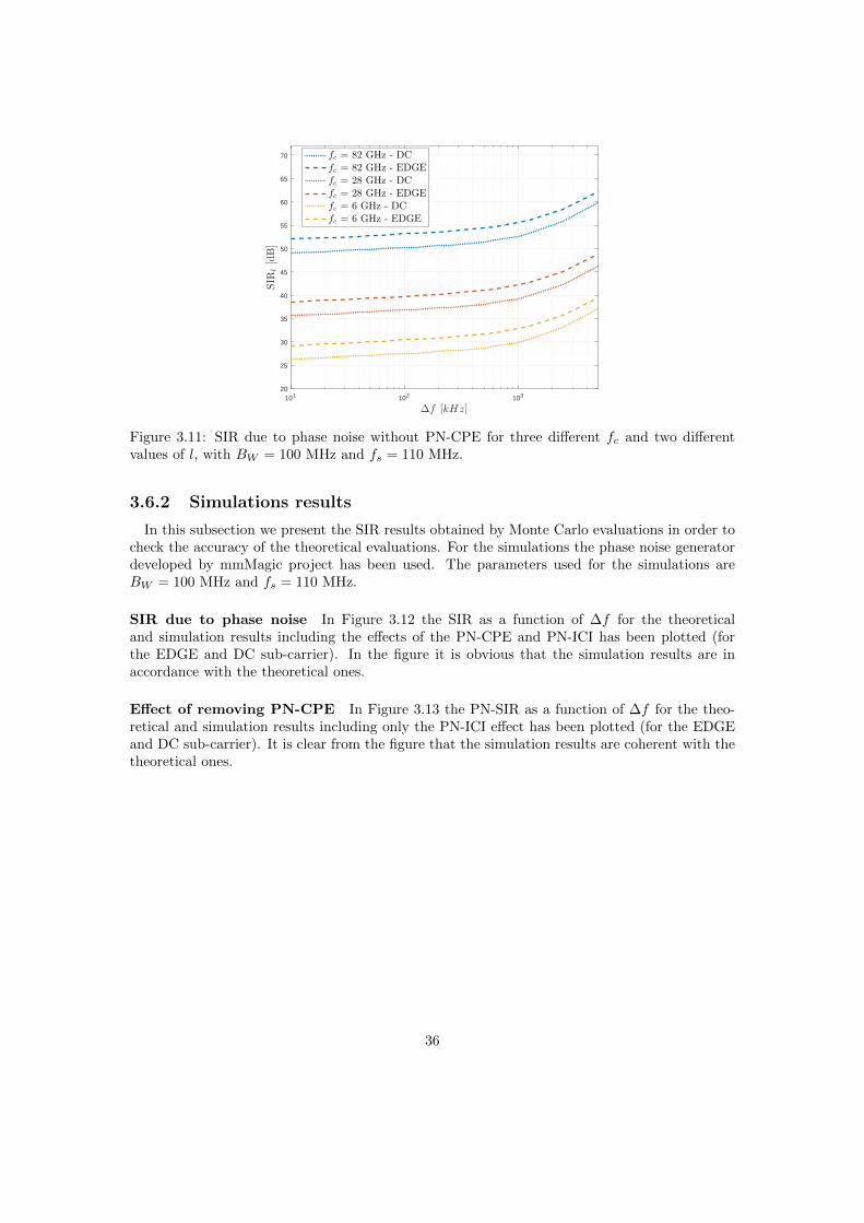
In OFDM the interference term produced by the PN-CPE is easily removed (as was explainedin Section 3.2). There are different methods to remove the PN-CPE (all of them make use ofpilot symbols) as the one presented in [14]. So, as the PN-CPE correction is an easy process, itmakes sense to study the effect of phase noise when PN-CPE is removed.

Effect of removing PN-CPE In Figure 3.11 the SIR as a function of ∆f including onlythe PN-ICI effect has been plotted (for the EDGE and DC sub-carrier). Removing the PN-CPEcontributions has a high impact in the SIR, specially for high sub-carrier spacings in which PNICIl

is quite low compared with PNCPEl. After removing the PN-CPE contribution, the SIR increases

when ∆f increases.

35

101 102 103

∆f [kHz]

20

25

30

35

40

45

50

55

60

65

70

SIR

l[dB]

fc = 82 GHz - DCfc = 82 GHz - EDGEfc = 28 GHz - DCfc = 28 GHz - EDGEfc = 6 GHz - DCfc = 6 GHz - EDGE

Figure 3.11: SIR due to phase noise without PN-CPE for three different fc and two differentvalues of l, with BW = 100 MHz and fs = 110 MHz.

3.6.2 Simulations results

In this subsection we present the SIR results obtained by Monte Carlo evaluations in order tocheck the accuracy of the theoretical evaluations. For the simulations the phase noise generatordeveloped by mmMagic project has been used. The parameters used for the simulations areBW = 100 MHz and fs = 110 MHz.

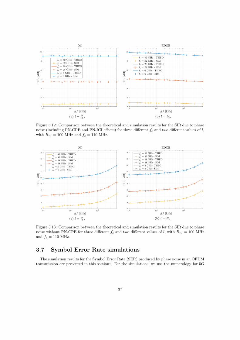
SIR due to phase noise In Figure 3.12 the SIR as a function of ∆f for the theoreticaland simulation results including the effects of the PN-CPE and PN-ICI has been plotted (forthe EDGE and DC sub-carrier). In the figure it is obvious that the simulation results are inaccordance with the theoretical ones.

Effect of removing PN-CPE In Figure 3.13 the PN-SIR as a function of ∆f for the theo-retical and simulation results including only the PN-ICI effect has been plotted (for the EDGEand DC sub-carrier). It is clear from the figure that the simulation results are coherent with thetheoretical ones.

36

101 102 103

∆f [kHz]

20

25

30

35

40

45

50

SIR

l[dB]

DC

fc = 82 GHz - THEOfc = 82 GHz - SIMfc = 28 GHz - THEOfc = 28 GHz - SIMfc = 6 GHz - THEOfc = 6 GHz - SIM

(a) l = N2

.

101 102 103

∆f [kHz]

20

25

30

35

40

45

50

SIR

l[dB]

EDGE

fc = 82 GHz - THEOfc = 82 GHz - SIMfc = 28 GHz - THEOfc = 28 GHz - SIMfc = 6 GHz - THEOfc = 6 GHz - SIM

(b) l = Ng

Figure 3.12: Comparison between the theoretical and simulation results for the SIR due to phasenoise (including PN-CPE and PN-ICI effects) for three different fc and two different values of l,with BW = 100 MHz and fs = 110 MHz.

101 102 103

∆f [kHz]

25

30

35

40

45

50

55

60

65

70

SIR

l[dB]

DC

fc = 82 GHz - THEOfc = 82 GHz - SIMfc = 28 GHz - THEOfc = 28 GHz - SIMfc = 6 GHz - THEOfc = 6 GHz - SIM

(a) l = N2

.

101 102 103

∆f [kHz]

25

30

35

40

45

50

55

60

65

70

SIR

l[dB]

EDGE

fc = 82 GHz - THEOfc = 82 GHz - SIMfc = 28 GHz - THEOfc = 28 GHz - SIMfc = 6 GHz - THEOfc = 6 GHz - SIM

(b) l = Ng .

Figure 3.13: Comparison between the theoretical and simulation results for the SIR due to phasenoise without PN-CPE for three different fc and two different values of l, with BW = 100 MHzand fs = 110 MHz.

3.7 Symbol Error Rate simulations

The simulation results for the Symbol Error Rate (SER) produced by phase noise in an OFDMtransmission are presented in this section1. For the simulations, we use the numerology for 5G

37

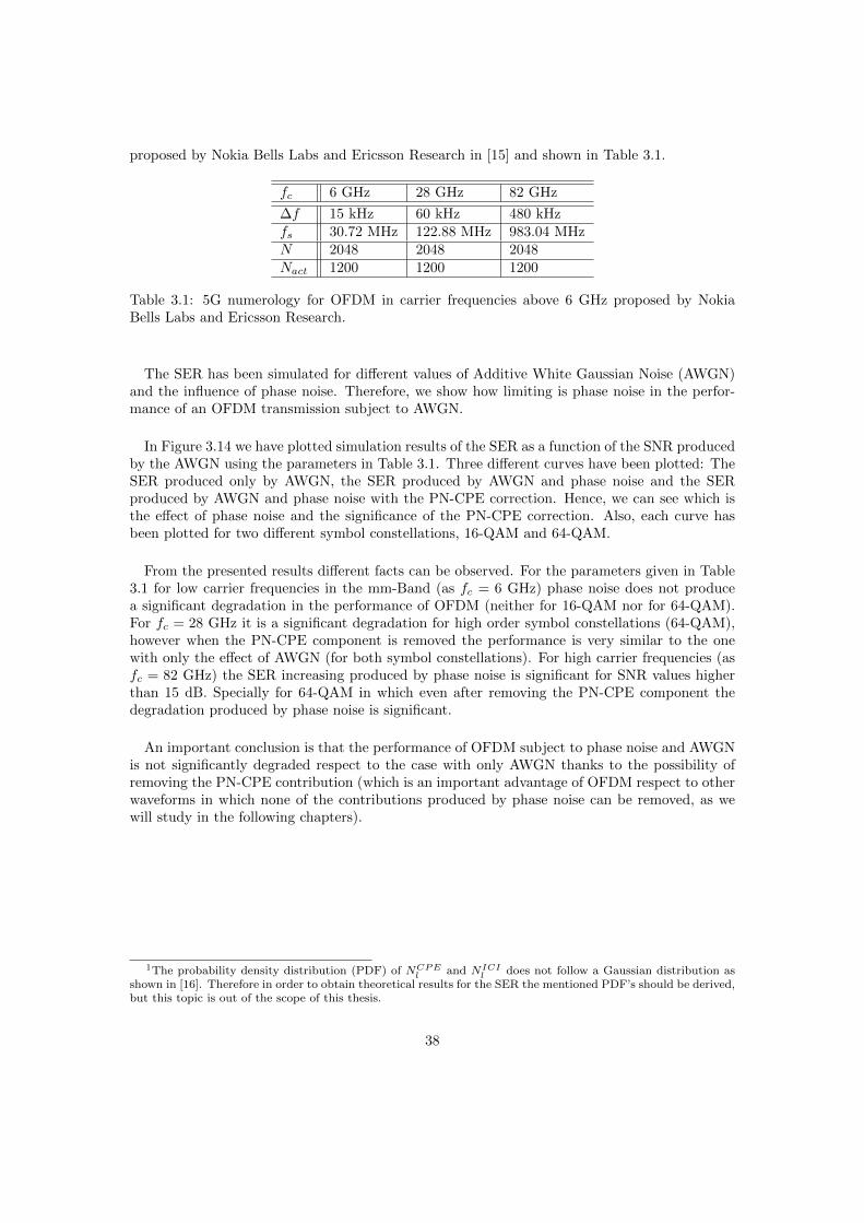
proposed by Nokia Bells Labs and Ericsson Research in [15] and shown in Table 3.1.

fc 6 GHz 28 GHz 82 GHz

∆f 15 kHz 60 kHz 480 kHzfs 30.72 MHz 122.88 MHz 983.04 MHzN 2048 2048 2048Nact 1200 1200 1200

Table 3.1: 5G numerology for OFDM in carrier frequencies above 6 GHz proposed by NokiaBells Labs and Ericsson Research.

The SER has been simulated for different values of Additive White Gaussian Noise (AWGN)and the influence of phase noise. Therefore, we show how limiting is phase noise in the perfor-mance of an OFDM transmission subject to AWGN.

In Figure 3.14 we have plotted simulation results of the SER as a function of the SNR producedby the AWGN using the parameters in Table 3.1. Three different curves have been plotted: TheSER produced only by AWGN, the SER produced by AWGN and phase noise and the SERproduced by AWGN and phase noise with the PN-CPE correction. Hence, we can see which isthe effect of phase noise and the significance of the PN-CPE correction. Also, each curve hasbeen plotted for two different symbol constellations, 16-QAM and 64-QAM.

From the presented results different facts can be observed. For the parameters given in Table3.1 for low carrier frequencies in the mm-Band (as fc = 6 GHz) phase noise does not producea significant degradation in the performance of OFDM (neither for 16-QAM nor for 64-QAM).For fc = 28 GHz it is a significant degradation for high order symbol constellations (64-QAM),however when the PN-CPE component is removed the performance is very similar to the onewith only the effect of AWGN (for both symbol constellations). For high carrier frequencies (asfc = 82 GHz) the SER increasing produced by phase noise is significant for SNR values higherthan 15 dB. Specially for 64-QAM in which even after removing the PN-CPE component thedegradation produced by phase noise is significant.

An important conclusion is that the performance of OFDM subject to phase noise and AWGNis not significantly degraded respect to the case with only AWGN thanks to the possibility ofremoving the PN-CPE contribution (which is an important advantage of OFDM respect to otherwaveforms in which none of the contributions produced by phase noise can be removed, as wewill study in the following chapters).

1The probability density distribution (PDF) of NCPEl and NICI

l does not follow a Gaussian distribution asshown in [16]. Therefore in order to obtain theoretical results for the SER the mentioned PDF’s should be derived,but this topic is out of the scope of this thesis.

38

10 15 20 25 30 35 40 45 50

SNR [dB]

10-6

10-5

10-4

10-3

10-2

10-1

100

SER

AWGN and PNAWGN and PN, PN-CPE removedAWGN

(a) fc = 6 GHz and 16-QAM.

10 15 20 25 30 35 40 45 50

SNR [dB]

10-6

10-5

10-4

10-3

10-2

10-1

100

SER

AWGN and PNAWGN and PN, PN-CPE removedAWGN

(b) fc = 6 GHz and 64-QAM.

10 15 20 25 30 35 40 45 50

SNR [dB]

10-6

10-5

10-4

10-3

10-2

10-1

100

SER

AWGN and PNAWGN and PN, PN-CPE removedAWGN

(c) fc = 28 GHz and 16-QAM.

10 15 20 25 30 35 40 45 50

SNR [dB]

10-6

10-5

10-4

10-3

10-2

10-1

100

SER

AWGN and PNAWGN and PN, PN-CPE removedAWGN

(d) fc = 28 GHz and 64-QAM.

10 15 20 25 30 35 40 45 50

SNR [dB]

10-6

10-5

10-4

10-3

10-2

10-1

100

SER

AWGN and PNAWGN and PN, PN-CPE removedAWGN

(e) fc = 82 GHz and 16-QAM.

10 15 20 25 30 35 40 45 50

SNR [dB]

10-6

10-5

10-4

10-3

10-2

10-1

100

SER

AWGN and PNAWGN and PN, PN-CPE removedAWGN

(f) fc = 82 GHz and 64-QAM.

Figure 3.14: Simulation results for the SER due to phase noise and AWGN for the parametersin Table 3.1.

39

Chapter 4

QAM-FBMC

Quadrature Amplitude Modulation - Filter-Bank Multi-carrier (QAM-FBMC) is anon-orthogonal MCM proposed for 5G as alternative to OFDM. Its main features were introducedin Section 2.1.2. This chapter presents the derivations and evaluations carried out in order tostudy the effects of phase noise in QAM-FBMC. Also the effects produced by the self-interferencespresented in Section 2.1.2 are studied. First we start deriving the expressions for the modulatedand demodulated signals. Next we study the effects of phase noise and self-interferences in thedemodulated signal, deriving expressions for the power of the interference terms. Following wederive the expressions for the Symbol-to-Interference Ratio (SIR). Once the expressions for theSIR are obtained, an analysis of the functions that determine the value of the SIR is carriedout (we refer to these functions as weighting functions). Finally, the SIR is evaluated for someconcrete implementation parameters.

4.1 Modulated and demodulated signal

Modulated signal The discrete time modulated signal for a QAM-FBMC symbol with Nsub-carriers follows the expression

x[n] =∑

d∈D

∑

i∈IXi,d pi[n− dN ] , (4.1)

where Xi,d is any symbol modulated in sub-carrier i and overlap index d, I is the set withthe index of active sub-carriers, D is the set with the index of the overlapping symbols (D =−K + 1, ...,K − 1) and pi[n] is the transmitter filter for sub-carrier i.

The filter for sub-carrier i is defined as

pi[n] :=

peven[n] ej2π

iN n if i is even

podd[n] ej2πiN n if i is odd

, (4.2)

where peven[n] and podd[n] are the base filters for even and odd sub-carriers respectively. Thebase filters are FIR filters with L = K N real-valued time coefficients and total energy equal to1, i.e.,

∑∞n=−∞ |peven[n]|2 =

∑∞n=−∞ |podd[n]|2 = 1.

40

Demodulated signal The demodulation is performed using the matched filter demodulation.So, the demodulated signal in sub-carrier l follows from (2.2) and it is given by

Rl = r[n] ∗ gl[n]

∣∣∣∣n=0

, (4.3)

in which r[n] is the sampled base-band received signal, ∗ is the convolution operator and gl[n] isthe matched filter for sub-carrier l, which is defined as

gl[n] := pi[−n] (4.4)

Note: Ideally the demodulation should produce Rl = Xl,0, however this equality is not possibledue to the intrinsic self-interferences of the waveform.

4.2 Demodulated signal subject to phase noise

The sampled base-band received signal with a sample rate fs subject to phase noise is givenby

r[n] = x[n] (1 + jφ[n]) , (4.5)

which follows from the sampled version of (2.18) while φ[n] is the sampled phase noise, defined

as φ[n] = φ(t)∣∣t= n

fs

.

The demodulated signal subject to phase noise follows

Rl(a)= r[n] ∗ gl[n]

∣∣∣∣n=0

(b)=[x[n]

(1 + jφ[n]

)]∗ gl[n]

∣∣∣∣n=0

(c)=

[∑

d∈D

∑

i∈IXi,d pi[n− dN ]

(1 + jφ[n]

)]∗ gl[n]

∣∣∣∣n=0

(d)=∑

d∈D

∑

i∈IXi,d

[pi[n− dN ] ∗ gl[n]

∣∣∣∣n=0

]+∑

d∈D

∑

i∈IXi,d

[jφ[n] pi[n− dN ] ∗ gl[n]

∣∣∣∣n=0

]

(e)=∑

d∈D

∑

i∈IXi,d λi,l,d +

∑

d∈D

∑

i∈IXi,d βi,l,d

(f)= Xl,0 +

∑

i∈IICIXi,0 λi,l,0 +

∑

d∈DISI

∑

i∈IXi,d λi,l,d +

+Xl,0 βl,l,0 +∑

i∈IICIXi,0 βi,l,0 +

∑

d∈DISI

∑

i∈IXi,d βi,l,d (4.6)

(a) follows from (4.3); (b) follows from (4.5); (c) follows from (4.1); (d) follows from the dis-tributivity property of the convolution; (e) follows by defining λi,l,d := pi[n−dN ]∗ gl[n]

∣∣n=0

and

βi,l,d := [jφ[n] pi[n− dN ]]∗gl[n]∣∣n=0

; (f) follows from separate the different terms according to itscause. Two new sets of indices have been introduced in (4.6), IICI = I\l and DISI = D\0,which contain the indices of the interfering sub-carriers and symbols respectively.

41

The terms in (4.6) that only depend on the impulse response of the filter are

λi,l,d = pi[n− dN ] ∗ gl[n]

∣∣∣∣n=0

(a)=

∞∑

s=−∞pi[s− dN ] gl[0− s]

(b)=

∞∑

s=−∞pi[s− dN ] pl[s] (4.7)

(a) follows from the convolution definition evaluated in n = 0; (b) follows from (4.4). It isimportant that ∀i ∈ I, ∀l ∈ I and ∀d ∈ D λi,l,d is a deterministic parameter.

An important result that has been applied in (4.6) related with the term in (4.7) is

λl,l,0 =

∞∑

s=−∞pl[s] pl[s] =

∑∞s=−∞ |peven[s]|2 = 1 if l even∑∞s=−∞ |podd[s]|

2= 1 if l odd

(4.8)

The terms in (4.6) that not only depend on the impulse response of the filter but also in phasenoise are

βi,l,d = [jφ[n] pi[n− dN ]]∗gl[n]

∣∣∣∣n=0

=

∞∑

s=−∞jφ[s]pi[s−dN ]gl[0−s] =

∞∑

s=−∞jφ[s]pi[s−dN ]pl[s]

(4.9)where the same steps than in (4.7) have been followed. In this case ∀i ∈ I, ∀l ∈ I and ∀d ∈ Dβi,l,d is a random variable because it depends on φ[n].

The expression in (4.6) can be rewritten by defining a interference term for each of the effectsproduced by self-interferences and phase noise

Rl = Xl,0 + IICIl + IISIl +NCPEl +N ICI

l +N ISIl , (4.10)

where IICIl , IISIl , NCPEl , N ICI

l and N ISIl are defined next from (4.11) to (4.15).

The interference terms in (4.10) can be classified according to its cause:

• Interference terms produced by self-interferences

IICIl :=∑

i∈IICIXi,0 λi,l,0 (4.11)

IISIl :=∑

d∈DISI

∑

i∈IXi,d λi,l,d (4.12)

which are the interference terms related with the effects presented in 2.1.2.

• Interference terms produced phase noise

NCPEl := Xl,0 βl,l,0 (4.13)

N ICIl :=

∑

i∈IICIXi,0 βi,l,0 (4.14)

N ISIl :=

∑

d∈DISI

∑

i∈IXi,d βi,l,d (4.15)

42

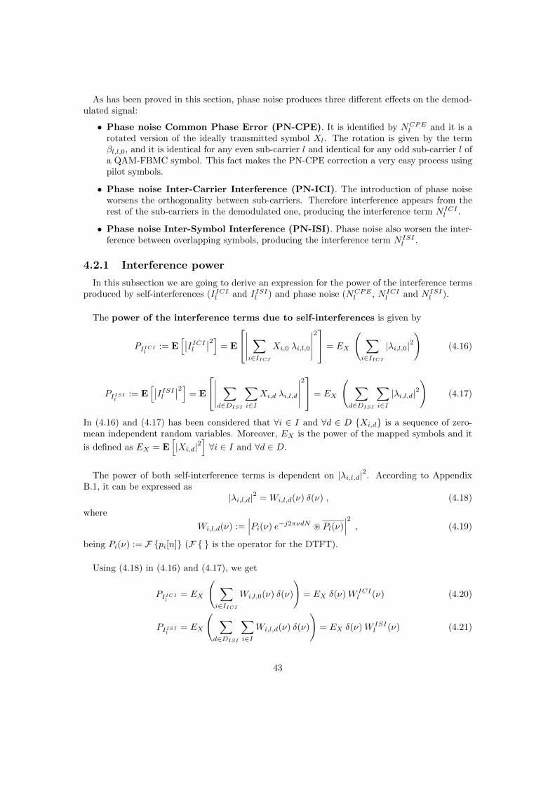
As has been proved in this section, phase noise produces three different effects on the demod-ulated signal:

• Phase noise Common Phase Error (PN-CPE). It is identified by NCPEl and it is a

rotated version of the ideally transmitted symbol Xl. The rotation is given by the termβl,l,0, and it is identical for any even sub-carrier l and identical for any odd sub-carrier l ofa QAM-FBMC symbol. This fact makes the PN-CPE correction a very easy process usingpilot symbols.

• Phase noise Inter-Carrier Interference (PN-ICI). The introduction of phase noiseworsens the orthogonality between sub-carriers. Therefore interference appears from therest of the sub-carriers in the demodulated one, producing the interference term N ICI

l .

• Phase noise Inter-Symbol Interference (PN-ISI). Phase noise also worsen the inter-ference between overlapping symbols, producing the interference term N ISI

l .

4.2.1 Interference power

In this subsection we are going to derive an expression for the power of the interference termsproduced by self-interferences (IICIl and IISIl ) and phase noise (NCPE

l , N ICIl and N ISI

l ).

The power of the interference terms due to self-interferences is given by

PIICIl:= E

[∣∣IICIl

∣∣2]

= E

∣∣∣∣∣∑

i∈IICIXi,0 λi,l,0

∣∣∣∣∣

2 = EX

( ∑

i∈IICI|λi,l,0|2

)(4.16)

PIISIl:= E

[∣∣IISIl

∣∣2]

= E

∣∣∣∣∣∑

d∈DISI

∑

i∈IXi,d λi,l,d

∣∣∣∣∣

2 = EX

( ∑

d∈DISI

∑

i∈I|λi,l,d|2

)(4.17)

In (4.16) and (4.17) has been considered that ∀i ∈ I and ∀d ∈ D Xi,d is a sequence of zero-mean independent random variables. Moreover, EX is the power of the mapped symbols and it

is defined as EX = E[|Xi,d|2

]∀i ∈ I and ∀d ∈ D.

The power of both self-interference terms is dependent on |λi,l,d|2. According to AppendixB.1, it can be expressed as

|λi,l,d|2 = Wi,l,d(ν) δ(ν) , (4.18)

where

Wi,l,d(ν) :=∣∣∣Pi(ν) e−j2πνdN ~ Pl(ν)

∣∣∣2

, (4.19)

being Pi(ν) := F pi[n] (F is the operator for the DTFT).

Using (4.18) in (4.16) and (4.17), we get

PIICIl= EX

( ∑

i∈IICIWi,l,0(ν) δ(ν)

)= EX δ(ν)W ICI

l (ν) (4.20)

PIISIl= EX

( ∑

d∈DISI

∑

i∈IWi,l,d(ν) δ(ν)

)= EX δ(ν)W ISI

l (ν) (4.21)

43

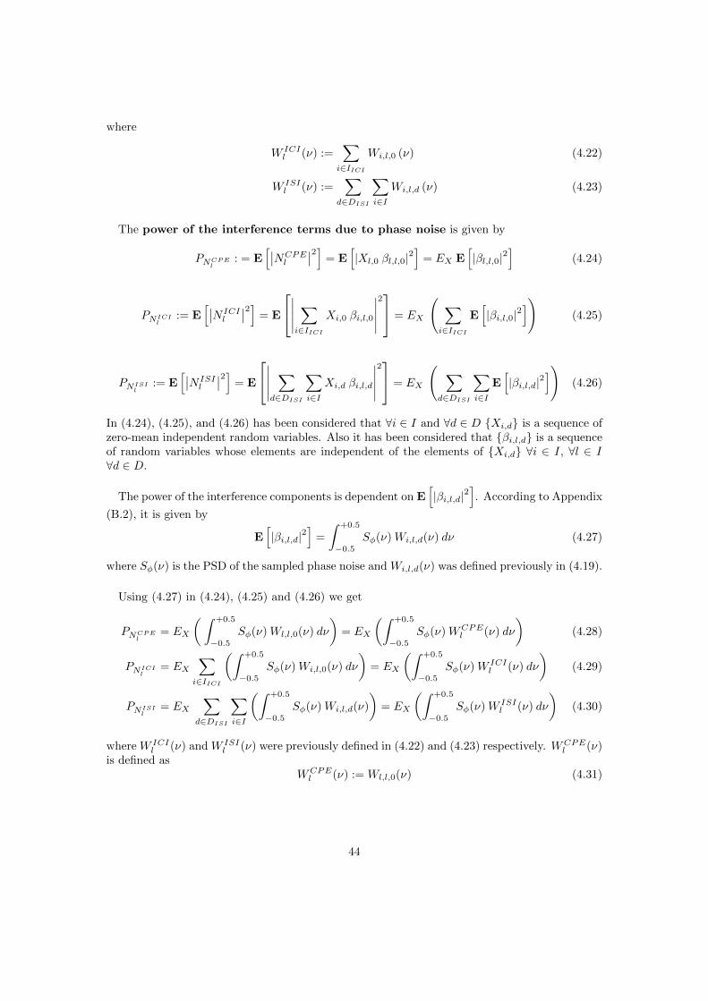
where

W ICIl (ν) :=

∑

i∈IICIWi,l,0 (ν) (4.22)

W ISIl (ν) :=

∑

d∈DISI

∑

i∈IWi,l,d (ν) (4.23)

The power of the interference terms due to phase noise is given by

PNCPEl: = E

[∣∣NCPEl

∣∣2]

= E[|Xl,0 βl,l,0|2

]= EX E

[|βl,l,0|2

](4.24)

PNICIl:= E

[∣∣N ICIl

∣∣2]

= E

∣∣∣∣∣∑

i∈IICIXi,0 βi,l,0

∣∣∣∣∣

2 = EX

( ∑

i∈IICIE[|βi,l,0|2

])(4.25)

PNISIl:= E

[∣∣N ISIl

∣∣2]

= E

∣∣∣∣∣∑

d∈DISI

∑

i∈IXi,d βi,l,d

∣∣∣∣∣

2 = EX

( ∑

d∈DISI

∑

i∈IE[|βi,l,d|2

])(4.26)

In (4.24), (4.25), and (4.26) has been considered that ∀i ∈ I and ∀d ∈ D Xi,d is a sequence ofzero-mean independent random variables. Also it has been considered that βi,l,d is a sequenceof random variables whose elements are independent of the elements of Xi,d ∀i ∈ I, ∀l ∈ I∀d ∈ D.

The power of the interference components is dependent on E[|βi,l,d|2

]. According to Appendix

(B.2), it is given by

E[|βi,l,d|2

]=

∫ +0.5

−0.5

Sφ(ν)Wi,l,d(ν) dν (4.27)

where Sφ(ν) is the PSD of the sampled phase noise and Wi,l,d(ν) was defined previously in (4.19).

Using (4.27) in (4.24), (4.25) and (4.26) we get

PNCPEl= EX

( ∫ +0.5

−0.5

Sφ(ν)Wl,l,0(ν) dν

)= EX

(∫ +0.5

−0.5

Sφ(ν)WCPEl (ν) dν

)(4.28)

PNICIl= EX

∑

i∈IICI

(∫ +0.5

−0.5

Sφ(ν)Wi,l,0(ν) dν

)= EX

(∫ +0.5

−0.5

Sφ(ν)W ICIl (ν) dν

)(4.29)

PNISIl= EX

∑

d∈DISI

∑

i∈I

(∫ +0.5

−0.5

Sφ(ν)Wi,l,d(ν)

)= EX

(∫ +0.5

−0.5

Sφ(ν)W ISIl (ν) dν

)(4.30)

where W ICIl (ν) and W ISI

l (ν) were previously defined in (4.22) and (4.23) respectively. WCPEl (ν)

is defined asWCPEl (ν) := Wl,l,0(ν) (4.31)

44

4.2.2 Signal-to-Interference Ratio

In this subsection the effect of self-interferences and phase noise in the Signal-to-InterferenceRatio (SIR) is studied. First, the expression with only the effect of self-interferences is derived.Next, the expression with both effects (self-interferences and phase noise) is obtained. Finally,we derive the expression for the SIR when the PN-CPE effect is removed.

SIR due to self-interferences From (4.10) the expression for the SIR in the demodulatedsignal in sub-carrier l produced by the self-interferences is easily. Taking into account only theinterference terms produced by the self-interferences (IICIl and IISIl ), the SIR is given by

SIRl =EX

PIICIl+ PIISIl

(a)=

1[W ICIl (ν) +W ISI

l (ν)]δ(ν)

(4.32)

(a) follows from (4.20) and (4.21). PIICIland PIISIl

are the power of the interferences producedby S-ICI and S-ISI. EX is the power of the transmitted symbol in sub-carrier l, it is defined as

EX := E[|Xl,0|2

].

SIR due to self-interferences and phase noise From (4.10) the expression for the SIR inthe demodulated signal in sub-carrier l produced by the combined effect of self-interferences andphase noise is obtained

SIRl =EX

PIICIl+ PIISIl

+ PNCPEl+ PNICIl

+ PNISIl

(a)=

1∫ +0.5

−0.5WCPEl (ν)Sφ(ν)dν +

∫ +0.5

−0.5

[W ICIl (ν) +W ISI

l (ν)]

[δ(ν) + Sφ(ν)] dν(4.33)

(a) follows from (4.20), (4.21), (4.28) , (4.29), and (4.30). PNCPEl, PNICIl

and PNISIlare the

power of PN-CPE, PN-ICI, and PN-ISI respectively.

Effect of removing PN-CPE Assuming that the PN-CPE effect is completely removed, theexpression for the SIR produced by the combined effect of self-interferences and phase noise insub-carrier l is given by

SIRl =EX

PIICIl+ PIISIl

+ PNICIl+ PNISIl

(a)=

1∫ +0.5

−0.5

[W ICIl +W ISI

l (ν)]

[δ(ν) + Sφ(ν)] dν(4.34)

(a) follows from (4.20), (4.21), (4.29) and (4.30).

4.3 Weighting functions

In Section 3.5 the concept of weighting function was presented. They are tools used in MCMcompute the level of the interferences produced by phase noise. In QAM-FBMC, the weightingfunctions are also used to compute the level of the interferences produced by self-interferences.

45

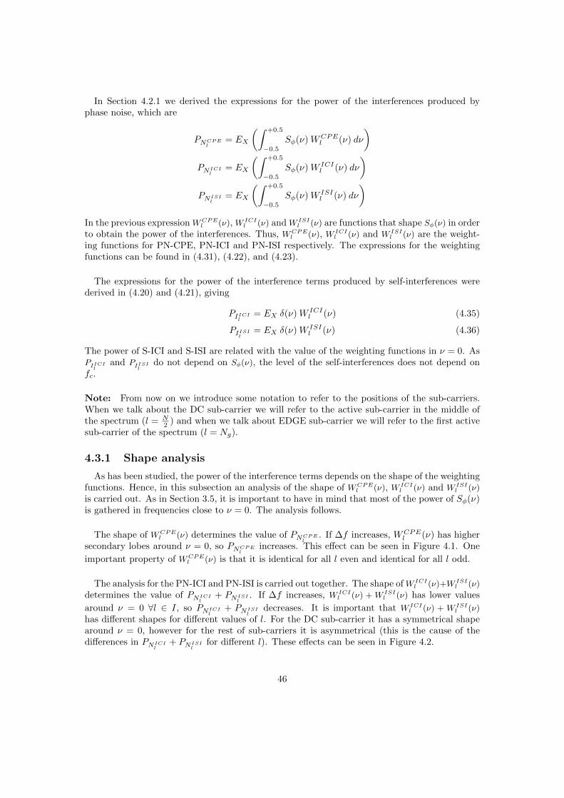
In Section 4.2.1 we derived the expressions for the power of the interferences produced byphase noise, which are

PNCPEl= EX

(∫ +0.5

−0.5

Sφ(ν)WCPEl (ν) dν

)

PNICIl= EX

(∫ +0.5

−0.5

Sφ(ν)W ICIl (ν) dν

)

PNISIl= EX

(∫ +0.5

−0.5

Sφ(ν)W ISIl (ν) dν

)

In the previous expression WCPEl (ν), W ICI

l (ν) and W ISIl (ν) are functions that shape Sφ(ν) in order

to obtain the power of the interferences. Thus, WCPEl (ν), W ICI

l (ν) and W ISIl (ν) are the weight-

ing functions for PN-CPE, PN-ICI and PN-ISI respectively. The expressions for the weightingfunctions can be found in (4.31), (4.22), and (4.23).

The expressions for the power of the interference terms produced by self-interferences werederived in (4.20) and (4.21), giving

PIICIl= EX δ(ν)W ICI

l (ν) (4.35)

PIISIl= EX δ(ν)W ISI

l (ν) (4.36)

The power of S-ICI and S-ISI are related with the value of the weighting functions in ν = 0. AsPIICIl

and PIISIl

do not depend on Sφ(ν), the level of the self-interferences does not depend onfc.

Note: From now on we introduce some notation to refer to the positions of the sub-carriers.When we talk about the DC sub-carrier we will refer to the active sub-carrier in the middle ofthe spectrum (l = N

2 ) and when we talk about EDGE sub-carrier we will refer to the first activesub-carrier of the spectrum (l = Ng).

4.3.1 Shape analysis

As has been studied, the power of the interference terms depends on the shape of the weightingfunctions. Hence, in this subsection an analysis of the shape of WCPE

l (ν), W ICIl (ν) and W ISI

l (ν)

is carried out. As in Section 3.5, it is important to have in mind that most of the power of Sφ(ν)is gathered in frequencies close to ν = 0. The analysis follows.

The shape of WCPEl (ν) determines the value of PNCPEl

. If ∆f increases, WCPEl (ν) has higher

secondary lobes around ν = 0, so PNCPElincreases. This effect can be seen in Figure 4.1. One

important property of WCPEl (ν) is that it is identical for all l even and identical for all l odd.

The analysis for the PN-ICI and PN-ISI is carried out together. The shape of W ICIl (ν)+W ISI

l (ν)

determines the value of PNICIl+ PNISIl

. If ∆f increases, W ICIl (ν) + W ISI

l (ν) has lower values

around ν = 0 ∀l ∈ I, so PNICIl+ PNISIl

decreases. It is important that W ICIl (ν) + W ISI

l (ν)

has different shapes for different values of l. For the DC sub-carrier it has a symmetrical shapearound ν = 0, however for the rest of sub-carriers it is asymmetrical (this is the cause of thedifferences in PNICIl

+ PNISIlfor different l). These effects can be seen in Figure 4.2.

46

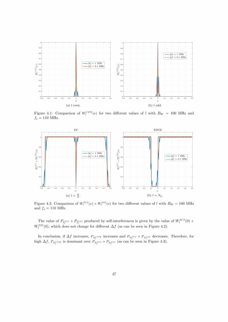
-0.5 -0.4 -0.3 -0.2 -0.1 0 0.1 0.2 0.3 0.4 0.5

ν

0

0.1

0.2

0.3

0.4

0.5

0.6

0.7

0.8

0.9

1

WCPE

l(ν) ∆f = 1 MHz

∆f = 0.1 MHz

(a) l even.

-0.5 -0.4 -0.3 -0.2 -0.1 0 0.1 0.2 0.3 0.4 0.5

ν

0

0.1

0.2

0.3

0.4

0.5

0.6

0.7

0.8

0.9

1

WCPE

l(ν)

∆f = 1 MHz∆f = 0.1 MHz

(b) l odd.

Figure 4.1: Comparison of WCPEl (ν) for two different values of l with BW = 100 MHz and

fs = 110 MHz.

-0.5 -0.4 -0.3 -0.2 -0.1 0 0.1 0.2 0.3 0.4 0.5

ν

0

0.2

0.4

0.6

0.8

1

WICI

l+W

ISI

l(ν)

DC

∆f = 1 MHz∆f = 0.1 MHz

(a) l = N2

.

-0.5 -0.4 -0.3 -0.2 -0.1 0 0.1 0.2 0.3 0.4 0.5

ν

0

0.2

0.4

0.6

0.8

1

WICI

l+W

ISI

l(ν)

EDGE

∆f = 1 MHz∆f = 0.1 MHz

(b) l = Ng .

Figure 4.2: Comparison of W ICIl (ν) +W ISI

l (ν) for two different values of l with BW = 100 MHzand fs = 110 MHz.

The value of PIICIl+ PIISIl

produced by self-interferences is given by the value of W ICIl (0) +

W ISIl (0), which does not change for different ∆f (as can be seen in Figure 4.2).

In conclusion, if ∆f increases, PNCPEl

increases and PNICIl

+ PNISIl

decreases. Therefore, for

high ∆f , PNCPEl

is dominant over PNICIl

+ PNISIl

(as can be seen in Figure 4.3).

47

101 102 103

∆f [kHz]

1

2

3

4

5

6

7

Pow

er[W

]

×10-4

PNCPEl

PN ICIl

+ PN ISIl

- DC

PN ICIl

+ PN ISIl

- EDGE

PNCPEl

+ PN ICIl

+ PN ISIl

- DC

PNCPEl

+ PN ICIl

+ PN ISIl

- EDGE

Figure 4.3: Power of the interference terms produced by phase noise with fc = 28 GHz, BW = 100MHz and fs = 110 MHz for two different sub-carrier locations.

4.4 Signal-to-Interference Ratio evaluations

In this section we evaluate the SIR using the derived expressions. The parameters BW = 100MHz and fs = 110 MHz have been used. The base filters proposed in [17] for K = 4 are the onesused to obtain the results. As in Chapter 3, the mmMagic project phase noise model introducedin Section 2.2 has been used.

SIR due to self-interferences In Figure 4.4 the SIR produced by the self-interferences (S-ICI and S-ISI) as a function of ∆f is shown. The difference in the SIR for the DC and EDGEsub-carriers is explained because in the EDGE sub-carrier one of the two closest neighbour sub-carriers is a null band, however in the DC sub-carrier both closest sub-carriers are not null bands.The closest neighbours are the sub-carriers that higher level of interference produce, so for theEDGE sub-carrier the interference level is lower. As was explained in Section 4.3, the level ofthe self-interferences is constant for different values of ∆f .

SIR due to self-interferences and phase noise Once the effect of the self-interferenceshas been studied, we present the evaluations with the combined effect of the self-interferencesand phase noise. In Figure 4.5 the SIR with the effects of self-interferences and phase noise as afunction of ∆f is shown. It can be seen how the effect of phase noise produces a decreasing inthe SIR respect to the case in Figure 4.4. One important fact is that the effect of phase noise isnot very significant because the power of the self-interferences is dominant. Only for high carrierfrequencies, where the PSD of phase noise has higher values, the decreasing produced by phasenoise in the SIR is significant.

Effect of removing PN-CPE As in the case of OFDM, in QAM-FBMC the interferenceterm produced by the CPE is easily removed because it is a rotated version of the transmittedsymbol. In Figure 4.6 the SIR with the effects of self-interferences and phase noise withoutPN-CPE as a function of ∆f is shown. Removing the effect of PN-CPE increases the SIR. The

48

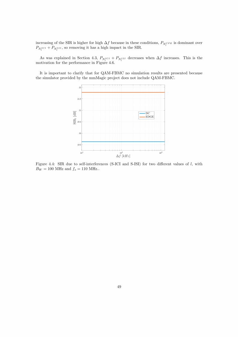
increasing of the SIR is higher for high ∆f because in these conditions, PNCPElis dominant over

PNICIl+ PNISIl

, so removing it has a high impact in the SIR.

As was explained in Section 4.3, PNICIl+ PNISIl

decreases when ∆f increases. This is themotivation for the performance in Figure 4.6.

It is important to clarify that for QAM-FBMC no simulation results are presented becausethe simulator provided by the mmMagic project does not include QAM-FBMC.

101 102 103

∆f [kHz]

19.5

20

20.5

21

21.5

22

SIR

l[dB]

DCEDGE

Figure 4.4: SIR due to self-interferences (S-ICI and S-ISI) for two different values of l, withBW = 100 MHz and fs = 110 MHz..

49

101 102 103

∆f [kHz]

17

17.5

18

18.5

19

19.5

20

20.5

21

21.5

22

SIR

l[dB]

DC

fc = 6 GHz

fc = 28 GHz

fc = 82 GHz

(a) l = N2

.

101 102 103

∆f [kHz]

17

17.5

18

18.5

19

19.5

20

20.5

21

21.5

22

SIR

l[dB]

EDGE

fc = 6 GHzfc = 28 GHzfc = 82 GHz

(b) l = Ng .

Figure 4.5: SIR due to self-interferences (S-ICI and S-ISI) and phase noise (PN-CPE, PN-ICIand PN-ISI) for three different fc and two different values of l, with BW = 100 MHz and fs = 110MHz.

101 102 103

∆f [kHz]

17

17.5

18

18.5

19

19.5

20

20.5

21

21.5

22

SIR

l[dB]

DC

fc = 6 GHz

fc = 28 GHz

fc = 82 GHz

(a) l = N2

.

101 102 103

∆f [kHz]

17

17.5

18

18.5

19

19.5

20

20.5

21

21.5

22

SIR

l[dB]

EDGE

fc = 6 GHz

fc = 28 GHz

fc = 82 GHz

(b) l = Ng .

Figure 4.6: SIR due to self-interferences (S-ICI and S-ISI) and phase noise after PN-CPE re-moving (PN-ICI and PN-ISI) for three different fc and two different values of l, with BW = 100MHz and fs = 110 MHz.

50

Chapter 5

OQAM-FBMC

Offset Quadrature Amplitude Modulation - Filter-Bank Multi-carrier(OQAM-FBMC) is a non-orthogonal MCM proposed as waveform for 5G which main featureswere introduced in Section 2.1.3. As in the case of OFDM and QAM-FBMC, it is very importantto study the robustness of OQAM-FBMC against phase noises. This chapter presents the deriva-tions and evaluations carried out in order to study the effects of phase noise in OQAM-FBMC.Also the effects produced by the self-interferences presented in the Section 2.1.3 are studied.First we start deriving the expressions for the modulated and demodulated signals. Next westudy the effects of phase noise and self-interferences in the demodulated signal, deriving ex-pressions for the power of the interference terms. Following we derive the expressions for theSymbol-to-Interference Ratio (SIR). Once the expressions for the SIR are obtained, an analysisof the functions that determine the value of the SIR is carried out (we refer to these functions asweighting functions). Finally, the SIR and SER are evaluated for some concrete implementationparameters.

5.1 Modulated and Demodulated signal

Modulated signal The discrete time modulated signal for an OQAM-FBMC symbol with Nsub-carriers is given by

x[n] =∑

d∈D

∑

i∈IXi,d θi,d pi

[n− dN

2

], (5.1)

where Xi,d is any mapped symbol in the real field which modulates sub-carrier i and overlapindex d (Xi,d ∈ R), θi,d := ji+d is the phase related with the offset-mapping of sub-carrier i andoverlap index d, I is the set with the indices of active sub-carriers, D is the set with the indicesof the overlapping symbols (D = −2K + 1, ..., 2K − 1) and pi[n] is the transmitter filter forsub-carrier i.

The expression for the filter in sub-carrier i is given by

pi[n] := p[n] ej2πiN n , (5.2)

in which p[n] is the base filter for OQAM-FBMC. It is a FIR filter with L := K N real-valued

time coefficients and total energy equal to 1, i.e.,∑+∞−∞ |p[n]|2 = 1.

51

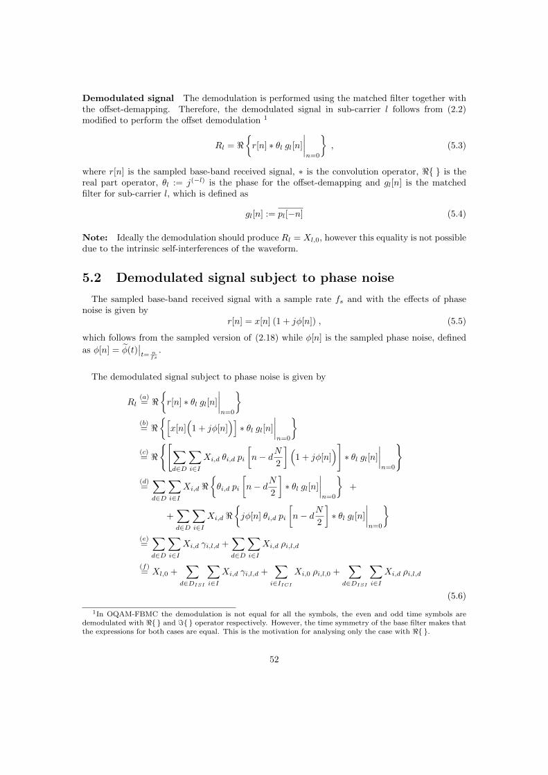
Demodulated signal The demodulation is performed using the matched filter together withthe offset-demapping. Therefore, the demodulated signal in sub-carrier l follows from (2.2)modified to perform the offset demodulation 1

Rl = <r[n] ∗ θl gl[n]

∣∣∣∣n=0

, (5.3)

where r[n] is the sampled base-band received signal, ∗ is the convolution operator, < is thereal part operator, θl := j(−l) is the phase for the offset-demapping and gl[n] is the matchedfilter for sub-carrier l, which is defined as

gl[n] := pl[−n] (5.4)

Note: Ideally the demodulation should produce Rl = Xl,0, however this equality is not possibledue to the intrinsic self-interferences of the waveform.

5.2 Demodulated signal subject to phase noise

The sampled base-band received signal with a sample rate fs and with the effects of phasenoise is given by

r[n] = x[n] (1 + jφ[n]) , (5.5)

which follows from the sampled version of (2.18) while φ[n] is the sampled phase noise, defined

as φ[n] = φ(t)∣∣t= n

fs

.

The demodulated signal subject to phase noise is given by

Rl(a)= <

r[n] ∗ θl gl[n]

∣∣∣∣n=0

(b)= <

[x[n]

(1 + jφ[n]

)]∗ θl gl[n]

∣∣∣∣n=0

(c)= <

[∑

d∈D

∑

i∈IXi,d θi,d pi

[n− dN

2

](1 + jφ[n]

)]∗ θl gl[n]

∣∣∣∣n=0

(d)=∑

d∈D

∑

i∈IXi,d <

θi,d pi

[n− dN

2

]∗ θl gl[n]

∣∣∣∣n=0

+

+∑

d∈D

∑

i∈IXi,d <

jφ[n] θi,d pi

[n− dN

2

]∗ θl gl[n]

∣∣∣∣n=0

(e)=∑

d∈D

∑

i∈IXi,d γi,l,d +

∑

d∈D

∑

i∈IXi,d ρi,l,d

(f)= Xl,0 +

∑

d∈DISI

∑

i∈IXi,d γi,l,d +

∑

i∈IICIXi,0 ρi,l,0 +

∑

d∈DISI

∑

i∈IXi,d ρi,l,d

(5.6)

1In OQAM-FBMC the demodulation is not equal for all the symbols, the even and odd time symbols aredemodulated with < and = operator respectively. However, the time symmetry of the base filter makes thatthe expressions for both cases are equal. This is the motivation for analysing only the case with < .

52

(a) follows from (5.3); (b) follows from (5.5); (c) follows from (5.1); (d) follows from the distribu-tivity property of both the convolution operator and the < operator ; (e) follows by definingγi,l,d := <

θi,d pi

[n− dN2

]∗ θlgl[n]

∣∣n=0

and ρi,l,d := <

jφ[n] θi,d pi

[n− dN2

]∗ θlgl[n]

∣∣n=0

;

(f) follows from separate the different terms according to its cause. Similarly to Chapter 4, twosets of indices have been introduced in (5.6), IICI = I\l and DISI = D\0, containing theindices of the interfering sub-carriers and symbols respectively.

The terms in (5.6) that only depend on the impulse response of the filters and the phase termsare

γi,l,d = <θi,d pi

[n− dN

2

]∗ θlgl[n]

∣∣n=0

(a)= <

∞∑

s=−∞θi,d pi

[s− dN

2

]θlgl[0− s]

(b)= <

∞∑

s=−∞θi,d pi

[s− dN

2

]θlpl[s]

(c)=

∞∑

s=−∞<θi,d pi

[s− dN

2

]θlpl[s]

(5.7)

(a) follows from the convolution evaluated in n = 0; (b) follows from (5.4); (c) follows fromthe distributivity property of < . It is important that ∀i ∈ I, ∀l ∈ I and ∀d ∈ D γi,l,d is adeterministic parameter.

An important result that has been applied in (5.6) related with the term in (5.7) is

γi,l,0(a)=

∞∑

s=−∞<θi,0 pi [s] θlpl[s]

(b)=

∞∑

s=−∞pi [s] pl[s]<

j(i−l)

= δi,l

(a) follows from (5.7); (b) follows from θi,0 θl = ji+0 j−l. The previous expression is alignedwith the state that OQAM-FBMC is not affected by S-ICI. In the previous expression δi,l is theKronecker delta. An important property applied in the previous derivation is that in OQAM-FBMC only neighbour sub-carriers overlap each other in the frequency domain.

The terms in (5.6) that not only depend on the impulse response of the filters and the phaseterms but also in phase noise are

ρi,l,d = <jφ[n] θi,d pi

[n− dN

2

]∗ θlgl[n]

∣∣n=0

= < ∞∑

s=−∞jφ[s] θi,d pi

[s− dN

2

]θlgl[0− s]

= < ∞∑

s=−∞jφ[s] θi,d pi

[s− dN

2

]θlpl[s]

=

∞∑

s=−∞<jφ[s] θi,d pi

[s− dN

2

]θlpl[s]

(5.8)

in which the same steps than in (5.7) have been followed. In this case, ∀l ∈ I and ∀d ∈ D ρi,l,dis a random variable because it depends on φ[n].

53

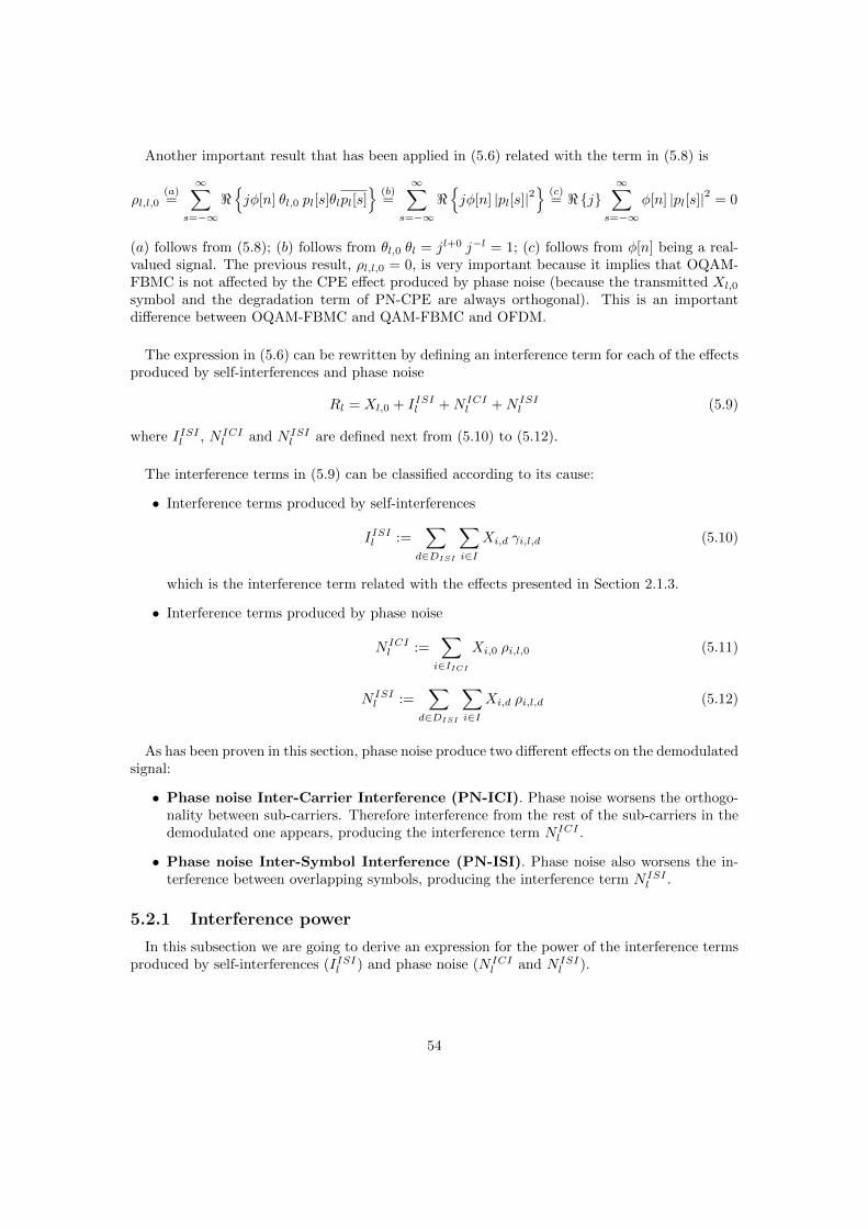
Another important result that has been applied in (5.6) related with the term in (5.8) is

ρl,l,0(a)=

∞∑

s=−∞<jφ[n] θl,0 pl[s]θlpl[s]

(b)=

∞∑

s=−∞<jφ[n] |pl[s]|2

(c)= <j

∞∑

s=−∞φ[n] |pl[s]|2 = 0

(a) follows from (5.8); (b) follows from θl,0 θl = jl+0 j−l = 1; (c) follows from φ[n] being a real-valued signal. The previous result, ρl,l,0 = 0, is very important because it implies that OQAM-FBMC is not affected by the CPE effect produced by phase noise (because the transmitted Xl,0

symbol and the degradation term of PN-CPE are always orthogonal). This is an importantdifference between OQAM-FBMC and QAM-FBMC and OFDM.

The expression in (5.6) can be rewritten by defining an interference term for each of the effectsproduced by self-interferences and phase noise

Rl = Xl,0 + IISIl +N ICIl +N ISI

l (5.9)

where IISIl , N ICIl and N ISI

l are defined next from (5.10) to (5.12).

The interference terms in (5.9) can be classified according to its cause:

• Interference terms produced by self-interferences

IISIl :=∑

d∈DISI

∑

i∈IXi,d γi,l,d (5.10)

which is the interference term related with the effects presented in Section 2.1.3.

• Interference terms produced by phase noise

N ICIl :=

∑

i∈IICIXi,0 ρi,l,0 (5.11)

N ISIl :=

∑

d∈DISI

∑

i∈IXi,d ρi,l,d (5.12)

As has been proven in this section, phase noise produce two different effects on the demodulatedsignal:

• Phase noise Inter-Carrier Interference (PN-ICI). Phase noise worsens the orthogo-nality between sub-carriers. Therefore interference from the rest of the sub-carriers in thedemodulated one appears, producing the interference term N ICI

l .

• Phase noise Inter-Symbol Interference (PN-ISI). Phase noise also worsens the in-terference between overlapping symbols, producing the interference term N ISI

l .

5.2.1 Interference power

In this subsection we are going to derive an expression for the power of the interference termsproduced by self-interferences (IISIl ) and phase noise (N ICI

l and N ISIl ).

54

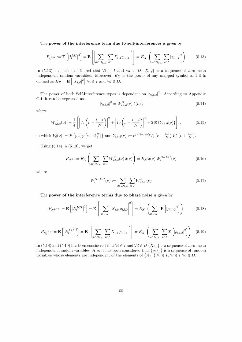
The power of the interference term due to self-interferences is given by

PIISIl:= E

[∣∣IISIl

∣∣2]

= E

∣∣∣∣∣∑

d∈DISI

∑

i∈IXi,dγi,l,d

∣∣∣∣∣

2 = EX

( ∑

d∈DISI

∑

i∈I|γi,l,d|2

)(5.13)

In (5.13) has been considered that ∀i ∈ I and ∀d ∈ D Xi,d is a sequence of zero-meanindependent random variables. Moreover, EX is the power of any mapped symbol and it is

defined as EX = E[|Xi,d|2

]∀i ∈ I and ∀d ∈ D.

The power of both Self-Interference types is dependent on |γi,l,d|2. According to AppendixC.1, it can be expressed as

|γi,l,d|2 = WSi,l,d(ν) δ(ν) , (5.14)

where

WSi,l,d(ν) :=

1

4

[∣∣∣∣Vd(ν − i− l

N

)∣∣∣∣2

+

∣∣∣∣Vd(ν +

i− lN

)∣∣∣∣2

+ 2 <Yi,l,d(ν)], (5.15)

in which Vd(ν) := Fp[s] p

[s− dN2

]and Yi,l,d(ν) := ejπ(i−l+d)Vd

(ν − i−l

N

)V ∗d(ν + i−l

N

).

Using (5.14) in (5.13), we get

PIISIl= EX

( ∑

d∈DISI

∑

i∈IWSi,l,d(ν) δ(ν)

)= EX δ(ν)WS−ISI

l (ν) (5.16)

where

WS−ISIl (ν) :=

∑

d∈DISI

∑

i∈IWSi,l,d (ν) (5.17)

The power of the interference terms due to phase noise is given by

PNICIl:= E

[∣∣N ICIl

∣∣2]

= E

∣∣∣∣∣∑

i∈IICIXi,0 ρi,l,0

∣∣∣∣∣

2 = EX

( ∑

i∈IICIE[|ρi,l,0|2

])(5.18)

PNISIl:= E

[∣∣N ISIl

∣∣2]

= E

∣∣∣∣∣∑

d∈DISI

∑

i∈IXi,d ρi,l,d

∣∣∣∣∣

2 = EX

( ∑

d∈DISI

∑

i∈IE[|ρi,l,d|2

])(5.19)

In (5.18) and (5.19) has been considered that ∀i ∈ I and ∀d ∈ D Xi,d is a sequence of zero-meanindependent random variables. Also it has been considered that ρi,l,d is a sequence of randomvariables whose elements are independent of the elements of Xi,d ∀i ∈ I, ∀l ∈ I ∀d ∈ D.

55

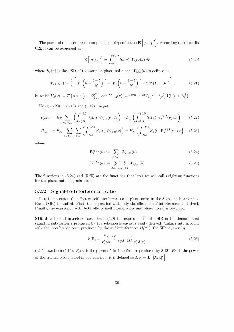
The power of the interference components is dependent on E[|ρi,l,d|2

]. According to Appendix

C.2, it can be expressed as

E[|ρi,l,d|2

]=

∫ +0.5

−0.5

Sφ(ν)Wi,l,d(ν) dν (5.20)

where Sφ(ν) is the PSD of the sampled phase noise and Wi,l,d(ν) is defined as

Wi,l,d(ν) :=1

4

[∣∣∣∣Vd(ν − i− l

N

)∣∣∣∣2

+

∣∣∣∣Vd(ν +

i− lN

)∣∣∣∣2

− 2 <Yi,l,d(ν)], (5.21)

in which Vd(ν) := Fp[s] p

[s− dN2

]and Yi,l,d(ν) := ejπ(i−l+d)Vd

(ν − i−l

N

)V ∗d(ν + i−l

N

).

Using (5.20) in (5.18) and (5.19), we get

PNICIl= EX

∑

i∈IICI

(∫ +0.5

−0.5

Sφ(ν)Wi,l,d(ν) dν

)= EX

(∫ +0.5

−0.5

Sφ(ν)W ICIl (ν) dν

)(5.22)

PNISIl= EX

∑

d∈DISI

∑

i∈I

(∫ +0.5

−0.5

Sφ(ν)Wi,l,d(ν)

)= EX

(∫ +0.5

−0.5

Sφ(ν)W ISIl (ν) dν

)(5.23)

where

W ICIl (ν) :=

∑

i∈IICIWi,l,0 (ν) (5.24)

W ISIl (ν) :=

∑

d∈DISI

∑

i∈IWi,l,d (ν) (5.25)

The functions in (5.24) and (5.25) are the functions that later we will call weighting functionsfor the phase noise degradations.

5.2.2 Signal-to-Interference Ratio

In this subsection the effect of self-interferences and phase noise in the Signal-to-InterferenceRatio (SIR) is studied. First, the expression with only the effect of self-interferences is derived.Finally, the expression with both effects (self-interferences and phase noise) is obtained.

SIR due to self-interferences From (5.9) the expression for the SIR in the demodulatedsignal in sub-carrier l produced by the self-interferences is easily derived. Taking into accountonly the interference term produced by the self-interferences (IISIl ), the SIR is given by

SIRl =EXPIISIl

(a)=

1

WS−ISIl (ν) δ(ν)

(5.26)

(a) follows from (5.16). PIISIlis the power of the interference produced by S-ISI. EX is the power

of the transmitted symbol in sub-carrier l, it is defined as EX := E[|Xl,0|2

].

56

SIR due to self-interferences and phase noise From (5.9) the expression for the SIR inthe demodulated signal in sub-carrier l produced by the combined effect of self-interferences andphase noise is obtained

SIRl(a)=

EXPIISIl

+ PNICIl+ PNISIl

(b)=

1

WS−ISIl (ν) δ(ν) +

∫ +0.5

−0.5

[W ICIl (ν) +W ISI

l (ν)]Sφ(ν) dν

(5.27)

(a) follows from (5.16), (5.22), and (5.23). PNISIland PNISIl

are the power of PN-ICI and PN-ISIrespectively.

5.3 Weighting functions

In Section 3.5 the concept of weighting function was presented. As was previously explained,they are tools used in MCM to compute the level of the interferences produced by phase noise.In OQAM-FBMC, contrary to QAM-FBMC, the weighting functions used for the phase noisedegradations can not be used for the self-interferences degradations.

In Section 5.2.1 we derived the expressions for the power of the interferences produced byphase noise, which were

PNICIl= EX

(∫ +0.5

−0.5

Sφ(ν)W ICIl (ν) dν

)

PNISIl= EX

(∫ +0.5

−0.5

Sφ(ν)W ISIl (ν) dν

)

In the previous expression W ICIl (ν) and W ISI

l (ν) are functions that shape Sφ(ν) in order to obtainthe power of the interferences. Thus, W ICI

l (ν) and W ISIl (ν) are the weighting functions for PN-

ICI and PN-ISI respectively. The expressions for the weighting functions can be found in (5.24)and (5.25).

Note: From now on we introduce some notation to refer to the positions of the sub-carriers.When we talk about the DC sub-carrier we refer to the active sub-carrier in the middle ofthe spectrum (l = N

2 ) and when we talk about EDGE sub-carrier we refer to the first activesub-carrier of the spectrum (l = Ng).

5.3.1 Shape analysis

As has been studied, the power of the interference terms depend on the shape of the weightingfunctions. Next we are going to analyse the shape of W ICI

l (ν) and W ISIl (ν). As in Section 3.5

and Section 4.3, it is important to have in mind that most of the power of Sφ(ν) is gathered infrequencies close to ν = 0. The analysis follows.

The shape of W ICIl (ν) determines the value of PNICI

l. If ∆f increases, the gap of W ICI

l (ν)

around ν = 0 is wider, so PNICIl

decreases ∀l ∈ I. This effect can be seen in Figure 5.1.

57

-0.5 -0.4 -0.3 -0.2 -0.1 0 0.1 0.2 0.3 0.4 0.5

ν

0

0.2

0.4

0.6

0.8

1

WICI

l(ν)

DC

∆f = 1 MHz∆f = 5 MHz

(a) l = N2

.

-0.5 -0.4 -0.3 -0.2 -0.1 0 0.1 0.2 0.3 0.4 0.5

ν

0

0.2

0.4

0.6

0.8

1

WICI

l(ν)

EDGE

∆f = 1 MHz

∆f = 5 MHz

(b) l = Ng .

Figure 5.1: Comparison of W ICIl (ν) for two different l, with BW = 100 MHz and fs = 110 MHz.

-0.5 -0.4 -0.3 -0.2 -0.1 0 0.1 0.2 0.3 0.4 0.5

ν

0

0.2

0.4

0.6

0.8

1

WISI

l,(ν)

DC

∆f = 1 MHz∆f = 5 MHz

(a) l = N2

.

-0.5 -0.4 -0.3 -0.2 -0.1 0 0.1 0.2 0.3 0.4 0.5

ν

0

0.2

0.4

0.6

0.8

1

WISI

l(ν)

EDGE

∆f = 1 MHz∆f = 5 MHz

(b) l = Ng .

Figure 5.2: Comparison of W ISIl (ν) for two different l, with BW = 100 MHz and fs = 110 MHz.

The value of PNISIl

is dependent on the shape of W ISIl (ν). If ∆f increases, the main lobe of

W ISIl (ν) around ν = 0 is wider, so PNISI

lincreases ∀l ∈ I. This effect can be seen in Figure 5.2.

One important property of W ICIl (ν) and W ISI

l (ν) is that they have different shapes for differentvalues of l, so PNICI

land PNISI

lalso have different values. We focus in the best and worst case

in terms of interference power (DC and EDGE sub-carrier respectively).

The shape of W ICIl (ν) + W ISI

l (ν) has been plotted in Figure 5.3. If ∆f increases, the valuesof W ICI

l (ν) + W ISIl (ν) for the DC sub-carrier around ν = 0 are not modified, so the change in

PNICIl

+PNISIl

is not significant. Contrary, in the EDGE sub-carrier the lobe of W ICIl (ν)+W ISI

l (ν)

58

around ν = 0 is wider, producing an increasing in PNICIl

+ PNISIl

.

-0.5 -0.4 -0.3 -0.2 -0.1 0 0.1 0.2 0.3 0.4 0.5

ν

0

0.2

0.4

0.6

0.8

1

WICI

l(ν)+

WISI

l(ν)

DC

∆f = 1 MHz

∆f = 5 MHz

(a) l = N2

.

-0.5 -0.4 -0.3 -0.2 -0.1 0 0.1 0.2 0.3 0.4 0.5

ν

0

0.2

0.4

0.6

0.8

1

WICI

l(ν)+

WISI

l(ν)

EDGE

∆f = 1 MHz∆f = 5 MHz

(b) l = Ng .

Figure 5.3: Comparison of W ICIl (ν) + W ISI

l (ν) for two different l, with BW = 100 MHz andfs = 110 MHz.

Summarizing, when ∆f increases PNISIl

increases and PNICIl

decreases ∀l ∈ I. Also, PNICIl

+

PNISIl

for the DC sub-carrier is nearly constant for different ∆f but for other sub-carriers itincreases if ∆f increases. These facts can be seen in Figure 5.4.

101 102 103

∆f [kHz]

0

1

2

3

4

5

6

7

Pow

er[W

]

×10-4

PN ICIl

+ PN ISIl

- DC

PN ICIl

+ PN ISIl

- EDGE

PN ISIl

- DC

PN ISIl

- EDGE

PN ICIl

- DC

PN ICIl

- EDGE

Figure 5.4: Power of the interference terms produced by phase noise for fc = 28 GHz, BW = 100MHz and fs = 110 MHz.

59

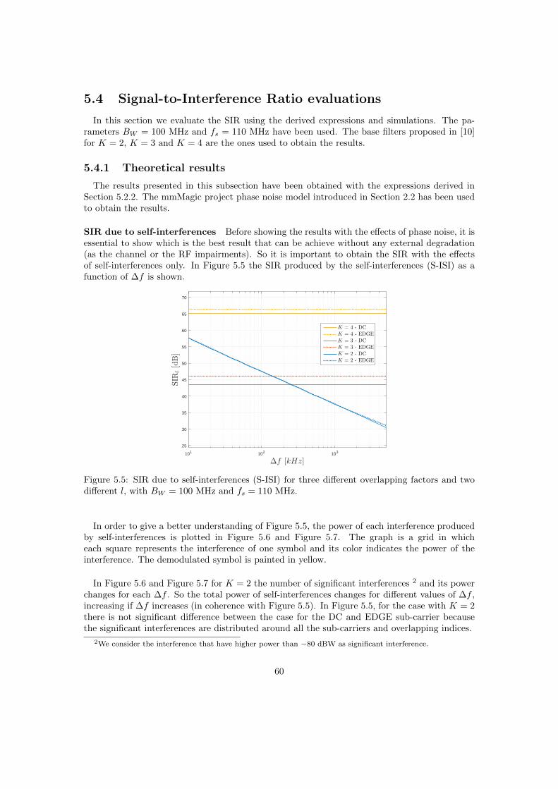
5.4 Signal-to-Interference Ratio evaluations

In this section we evaluate the SIR using the derived expressions and simulations. The pa-rameters BW = 100 MHz and fs = 110 MHz have been used. The base filters proposed in [10]for K = 2, K = 3 and K = 4 are the ones used to obtain the results.

5.4.1 Theoretical results

The results presented in this subsection have been obtained with the expressions derived inSection 5.2.2. The mmMagic project phase noise model introduced in Section 2.2 has been usedto obtain the results.

SIR due to self-interferences Before showing the results with the effects of phase noise, it isessential to show which is the best result that can be achieve without any external degradation(as the channel or the RF impairments). So it is important to obtain the SIR with the effectsof self-interferences only. In Figure 5.5 the SIR produced by the self-interferences (S-ISI) as afunction of ∆f is shown.

101 102 103

∆f [kHz]

25

30

35

40

45

50

55

60

65

70

SIR

l[dB]

K = 4 - DCK = 4 - EDGEK = 3 - DCK = 3 - EDGEK = 2 - DCK = 2 - EDGE

Figure 5.5: SIR due to self-interferences (S-ISI) for three different overlapping factors and twodifferent l, with BW = 100 MHz and fs = 110 MHz.

In order to give a better understanding of Figure 5.5, the power of each interference producedby self-interferences is plotted in Figure 5.6 and Figure 5.7. The graph is a grid in whicheach square represents the interference of one symbol and its color indicates the power of theinterference. The demodulated symbol is painted in yellow.

In Figure 5.6 and Figure 5.7 for K = 2 the number of significant interferences 2 and its powerchanges for each ∆f . So the total power of self-interferences changes for different values of ∆f ,increasing if ∆f increases (in coherence with Figure 5.5). In Figure 5.5, for the case with K = 2there is not significant difference between the case for the DC and EDGE sub-carrier becausethe significant interferences are distributed around all the sub-carriers and overlapping indices.

2We consider the interference that have higher power than −80 dBW as significant interference.

60

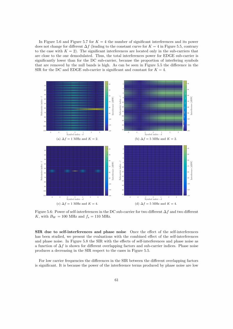
In Figure 5.6 and Figure 5.7 for K = 4 the number of significant interferences and its powerdoes not change for different ∆f (leading to the constant curve for K = 4 in Figure 5.5, contraryto the case with K = 2). The significant interferences are located only in the sub-carriers thatare close to the one demodulated. Thus, the total interferences power for EDGE sub-carrier issignificantly lower than for the DC sub-carrier, because the proportion of interfering symbolsthat are removed by the null bands is high. As can be seen in Figure 5.5 the difference in theSIR for the DC and EDGE sub-carrier is significant and constant for K = 4.

-3 -2 -1 0 1 2 3

Symbol index - d

10

20

30

40

50

60

70

80

90

100

110

Subcarrierindex

-l

-120

-110

-100

-90

-80

-70

-60

-50

-40

Interferen

ce[dBW

]

(a) ∆f = 1 MHz and K = 2.

-3 -2 -1 0 1 2 3

Symbol index - d

2

4

6

8

10

12

14

16

18

20

22

Subcarrierindex

-l

-120

-110

-100

-90

-80

-70

-60

-50

-40

Interferen

ce[dBW

]

(b) ∆f = 5 MHz and K = 2.

-6 -4 -2 0 2 4 6

Symbol index - d

10

20

30

40

50

60

70

80

90

100

110

Subcarrierindex

-l

-120

-110

-100

-90

-80

-70

-60

-50

-40

Interferen

ce[dBW

]

(c) ∆f = 1 MHz and K = 4.

-6 -4 -2 0 2 4 6

Symbol index - d

2

4

6

8

10

12

14

16

18

20

22

Subcarrierindex

-l

-120

-110

-100

-90

-80

-70

-60

-50

-40

Interferen

ce[dBW

]

(d) ∆f = 5 MHz and K = 4.

Figure 5.6: Power of self-interferences in the DC sub-carrier for two different ∆f and two differentK, with BW = 100 MHz and fs = 110 MHz.

SIR due to self-interferences and phase noise Once the effect of the self-interferenceshas been studied, we present the evaluations with the combined effect of the self-interferencesand phase noise. In Figure 5.8 the SIR with the effects of self-interferences and phase noise asa function of ∆f is shown for different overlapping factors and sub-carrier indices. Phase noiseproduces a decreasing in the SIR respect to the cases in Figure 5.5.

For low carrier frequencies the differences in the SIR between the different overlapping factorsis significant. It is because the power of the interference terms produced by phase noise are low

61

-3 -2 -1 0 1 2 3

Symbol index - d

10

20

30

40

50

60

70

80

90

100

110

Subcarrierindex

-l

-120

-110

-100

-90

-80

-70

-60

-50

-40

Interferen

ce[dBW

]

(a) ∆f = 1 MHz and K = 2.

-3 -2 -1 0 1 2 3

Symbol index - d

2

4

6

8

10

12

14

16

18

20

22

Subcarrierindex

-l

-120

-110

-100

-90

-80

-70

-60

-50

-40

Interferen

ce[dBW

]

(b) ∆f = 5 MHz and K = 2.

-6 -4 -2 0 2 4 6

Symbol index - d

10

20

30

40

50

60

70

80

90

100

110

Subcarrierindex

-l

-120

-110

-100

-90

-80

-70

-60

-50

-40Interferen

ce[dBW

]

(c) ∆f = 1 MHz and K = 4.

-6 -4 -2 0 2 4 6

Symbol index - d

2

4

6

8

10

12

14

16

18

20

22

Subcarrierindex

-l

-120

-110

-100

-90

-80

-70

-60

-50

-40

Interferen

ce[dBW

]

(d) ∆f = 5 MHz and K = 4.

Figure 5.7: Power of self-interferences in the EDGE sub-carrier for two different ∆f and twodifferent K, with BW = 100 MHz and fs = 110 MHz.

in comparison to the power of the interferences produced by self-interferences. However, for highfrequencies (as 82 GHz), the power of the interferences produced by phase noise are dominantover the ones produced by self-interferences, resulting in very similar SIR results for the threeoverlapping factors (because the power of the interference produced by phase noise is similar forthe three cases, but not the power of the interferences produced by self-interferences).

62

101 102 103

∆f [kHz]

20

25

30

35

40

45

50SIR

l[dB]

DC

fc = 6 GHz

fc = 28 GHz

fc = 82 GHz

(a) K = 2.

101 102 103

∆f [kHz]

20

25

30

35

40

45

50

SIR

l[dB]

EDGE

fc = 6 GHzfc = 28 GHzfc = 82 GHz

(b) K = 2.

101 102 103

∆f [kHz]

20

25

30

35

40

45

50

SIR

l[dB]

DC

fc = 6 GHz

fc = 28 GHz

fc = 82 GHz

(c) K = 3.

101 102 103

∆f [kHz]

20

25

30

35

40

45

50

SIR

l[dB]

EDGE

fc = 6 GHzfc = 28 GHzfc = 82 GHz

(d) K = 3.

101 102 103

∆f [kHz]

20

25

30

35

40

45

50

SIR

l[dB]

DC

fc = 6 GHz

fc = 28 GHz

fc = 82 GHz

(e) K = 4.

101 102 103

∆f [kHz]

20

25

30

35

40

45

50

SIR

l[dB]

EDGE

fc = 6 GHz

fc = 28 GHz

fc = 82 GHz

(f) K = 4.

Figure 5.8: SIR due to self-interferences (S-ISI) and phase noise (PN-ICI and PN-ISI) for threedifferent fc and three different overlapping factors for the DC and EDGE sub-carrier, withBW = 100 MHz and fs = 110 MHz.

63

5.4.2 Simulation results

The results presented in this subsection have been obtained by Monte Carlo evaluations usingthe phase noise generator developed by mmMagic project. The simulation results have beenobtained in order to check the accuracy of the theoretical evaluations.

SIR due to self-interferences In Figure 5.10 the SIR as a function of ∆f for the theoreticaland simulation results including the effects of self-interferences. In the figure it is obvious thatthe simulation results are in accordance with the theoretical ones.

101 102 103

∆f [kHz]

30

35

40

45

50

55

60

65

70

SIR

l[dB]

DC

K = 4 - THEOK = 4 - SIMK = 3 - THEOK = 3 - SIMK = 2 - THEOK = 2 - SIM

(a) l = N2

.

101 102 103

∆f [kHz]

30

35

40

45

50

55

60

65

70

SIR

l[dB]

EDGE

K = 4 - THEOK = 4 - SIMK = 3 - THEOK = 3 - SIMK = 2 - THEOK = 2 - SIM

(b) l = Ng .

Figure 5.9: Comparison between the theoretical and simulation results for the SIR due to self-interferences (S-ISI) for three different overlapping factors and for the DC and EDGE sub-carrier,with BW = 100 MHz and fs = 110 MHz.

SIR due to self-interferences and phase noise In Figure 5.10 the SIR as a function of∆f for the theoretical and simulation results including the effects of self-interferences and phasenoise. In the figure it is clear that the simulation results are in accordance with the theoreticalones.

64

101 102 103

∆f [kHz]

20

25

30

35

40

45

50

55SIR

l[dB]

DC

fc = 6 GHz - THEOfc = 6 GHz - SIMfc = 28 GHz - THEOfc = 28 GHz - SIMfc = 82 GHz - THEOfc = 82 GHz - SIM

(a) K = 2.

101 102 103

∆f [kHz]

20

25

30

35

40

45

50

55

SIR

l[dB]

EDGE

fc = 6 GHz - THEOfc = 6 GHz - SIMfc = 28 GHz - THEOfc = 28 GHz - SIMfc = 82 GHz - THEOfc = 82 GHz - SIM

(b) K = 2.

101 102 103

∆f [kHz]

20

25

30

35

40

45

50

55

SIR

l[dB]

DC

fc = 6 GHz - THEOfc = 6 GHz - SIMfc = 28 GHz - THEOfc = 28 GHz - SIMfc = 82 GHz - THEOfc = 82 GHz - SIM

(c) K = 3.

101 102 103

∆f [kHz]

20

25

30

35

40

45

50

55

SIR

l[dB]

EDGE

fc = 6 GHz - THEOfc = 6 GHz - SIMfc = 28 GHz - THEOfc = 28 GHz - SIMfc = 82 GHz - THEOfc = 82 GHz - SIM

(d) K = 3.

101 102 103

∆f [kHz]

20

25

30

35

40

45

50

55

SIR

l[dB]

DC

fc = 6 GHz - THEOfc = 6 GHz - SIMfc = 28 GHz - THEOfc = 28 GHz - SIMfc = 82 GHz - THEOfc = 82 GHz - SIM

(e) K = 4.

101 102 103

∆f [kHz]

20

25

30

35

40

45

50

55

SIR

l[dB]

EDGE

fc = 6 GHz - THEOfc = 6 GHz - SIMfc = 28 GHz - THEOfc = 28 GHz - SIMfc = 82 GHz - THEOfc = 82 GHz - SIM

(f) K = 4.

Figure 5.10: Comparison between the theoretical and simulation results for the SIR due to self-interferences (S-ISI) and phase noise (PN-ICI and PN-ISI) for three different fc and three differentoverlapping factors for the DC and EDGE sub-carrier, with BW = 100 MHz and fs = 110 MHz.

65

5.5 Symbol Error Rate evaluations

In this section we present the simulation evaluations for the Symbol Error Rate (SER) producedby phase noise. For the simulations we use the numerology presented in [15] and shown in Table5.1, as in Chapter 3. The SER has been simulated for different values of AWGN and the influenceof phase noise and self-interferences.

fc 6 GHz 28 GHz 82 GHz

∆f 15 kHz 60 kHz 480 kHzfs 30.72 MHz 122.88 MHz 983.04 MHzN 2048 2048 2048Nact 1200 1200 1200

Table 5.1: 5G numerology in frequencies above 6 GHz proposed by Nokia Bells Labs and EricssonResearch.

In Figure 5.11 we have plotted the results of the simulations of the SER as a function of theSNR produced by the AWGN using the parameters in Table 5.1. Two different curves have beenplotted: the SER produced by AWGN and self-interferences and the SER produced by AWGN,self-interferences and phase noise. Each curve has been plotted for K = 2 and K = 4, which arethe best overlapping factors in terms of achievable SIR. Also, two different symbol constellationshave been used, 16-QAM and 64-QAM.

From the presented evaluations different facts can be observed. For the parameters in Table5.1, for low carrier frequencies in the mm-Band (as fc = 6 GHz) phase noise does not producea significant degradation in the performance of OQAM-FBMC (neither for 16-QAM nor for 64-QAM). For fc = 28 GHz it is a significant degradation for high order symbol constellations(64-QAM) in values of SNR higher than 20 dB. For high carrier frequencies (as fc = 82 GHz)the SER increasing produced by phase noise is significant for both symbol constellations in SNRvalues higher than 15 dB, specially for 64-QAM.

The evaluation results show how the differences in the performance for K = 2 and K = 4 arenot very significant. Only for the case of Figure 5.11d the differences between both cases aresignificant, being the performance of the case with K = 4 slightly better than with K = 2.

66

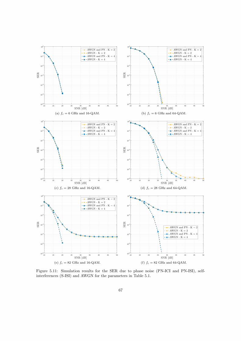
10 15 20 25 30 35 40 45 50

SNR [dB]

10-6

10-5

10-4

10-3

10-2

10-1

100

SER

AWGN and PN - K = 2

AWGN - K = 2

AWGN and PN - K = 4

AWGN - K = 4

(a) fc = 6 GHz and 16-QAM.

10 15 20 25 30 35 40 45 50

SNR [dB]

10-6

10-5

10-4

10-3

10-2

10-1

100

SER

AWGN and PN - K = 2

AWGN - K = 2

AWGN and PN - K = 4

AWGN - K = 4

(b) fc = 6 GHz and 64-QAM.

10 15 20 25 30 35 40 45 50

SNR [dB]

10-6

10-5

10-4

10-3

10-2

10-1

100

SER

AWGN and PN - K = 2

AWGN - K = 2

AWGN and PN - K = 4

AWGN - K = 4

(c) fc = 28 GHz and 16-QAM.

10 15 20 25 30 35 40 45 50

SNR [dB]

10-6

10-5

10-4

10-3

10-2

10-1

100

SER

AWGN and PN - K = 2

AWGN - K = 2

AWGN and PN - K = 4

AWGN - K = 4

(d) fc = 28 GHz and 64-QAM.

10 15 20 25 30 35 40 45 50

SNR [dB]

10-6

10-5

10-4

10-3

10-2

10-1

100

SER

AWGN and PN - K = 2

AWGN - K = 2

AWGN and PN - K = 4

AWGN - K = 4

(e) fc = 82 GHz and 16-QAM.

10 15 20 25 30 35 40 45 50

SNR [dB]

10-6

10-5

10-4

10-3

10-2

10-1

100

SER

AWGN and PN - K = 2

AWGN - K = 2

AWGN and PN - K = 4

AWGN - K = 4

(f) fc = 82 GHz and 64-QAM.

Figure 5.11: Simulation results for the SER due to phase noise (PN-ICI and PN-ISI), self-interferences (S-ISI) and AWGN for the parameters in Table 5.1.

67

Chapter 6

Comparison of waveforms subjectto phase noise

In Chapters 3, 4, and 5 we derived weighting functions to evaluate the effects of phase noisein OFDM, QAM-FBMC, and OQAM-FBMC, respectively. At the end of each chapter theseweighting functions were used to evaluate the performance of the three waveforms using commonparameters. In this chapter we use the obtained results to compare the effects of phase noisein the studied waveforms and determine which one offers better performance for the mmMagicphase noise model.

On the one hand, we will compare the achievable SIR after PN-CPE compensation. It is themost relevant case since PN-CPE is easily removed using pilot symbols, without increasing thecomplexity or the overhead of the system (because pilot symbols are needed anyway for channelestimation). It is important that OQAM-FBMC is not affected by PN-CPE, as explained inChapter 5. On the other hand, we will compare the achievable SIR after PN-CPE compensationwithout taking into account the effect of self-interferences. This case shows which is the trueeffect of phase noise in the achievable SIR (because it does not show the degradations due to thenon-orthogonalities of QAM-FBMC and OQAM-FBMC).

Achievable SIR after PN-CPE compensation In Figure 6.1 we show a comparison of theachievable SIR after PN-CPE compensation for the three waveforms. It includes the effect ofphase noise, but also the effect of the self-interferences for the non-orthogonal waveforms (QAM-FBMC and OQAM-FBMC). In the graph it can be seen how QAM-FBMC offers the worstperformance in all the cases, mainly because its high level of self-interferences. For the caseof OQAM-FBMC, we can find big differences in the performance for each overlapping factor.These differences are produced by the different level of self-interferences that OQAM-FBMChas for each overlapping factor (as studied in Chapter 5). The case with K = 4 outperformsthe cases with K = 2 and K = 3. Finally, it can be seen that OFDM outperforms QAM-FBMC and OQAM-FBMC, mainly because it is an orthogonal MCM which is not affected byself-interferences, but also because it offers a very good sensitivity against phase noise (as wewill show next).

Achievable SIR after PN-CPE compensation excluding Self-Interefences In Fig-ure 6.2 we have plotted a comparison of the achievable SIR after PN-CPE compensation ex-

68

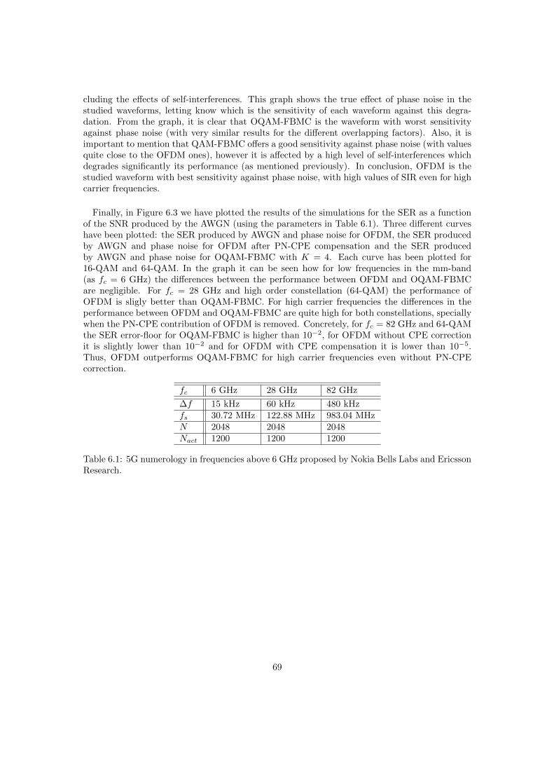
cluding the effects of self-interferences. This graph shows the true effect of phase noise in thestudied waveforms, letting know which is the sensitivity of each waveform against this degra-dation. From the graph, it is clear that OQAM-FBMC is the waveform with worst sensitivityagainst phase noise (with very similar results for the different overlapping factors). Also, it isimportant to mention that QAM-FBMC offers a good sensitivity against phase noise (with valuesquite close to the OFDM ones), however it is affected by a high level of self-interferences whichdegrades significantly its performance (as mentioned previously). In conclusion, OFDM is thestudied waveform with best sensitivity against phase noise, with high values of SIR even for highcarrier frequencies.

Finally, in Figure 6.3 we have plotted the results of the simulations for the SER as a functionof the SNR produced by the AWGN (using the parameters in Table 6.1). Three different curveshave been plotted: the SER produced by AWGN and phase noise for OFDM, the SER producedby AWGN and phase noise for OFDM after PN-CPE compensation and the SER producedby AWGN and phase noise for OQAM-FBMC with K = 4. Each curve has been plotted for16-QAM and 64-QAM. In the graph it can be seen how for low frequencies in the mm-band(as fc = 6 GHz) the differences between the performance between OFDM and OQAM-FBMCare negligible. For fc = 28 GHz and high order constellation (64-QAM) the performance ofOFDM is sligly better than OQAM-FBMC. For high carrier frequencies the differences in theperformance between OFDM and OQAM-FBMC are quite high for both constellations, speciallywhen the PN-CPE contribution of OFDM is removed. Concretely, for fc = 82 GHz and 64-QAMthe SER error-floor for OQAM-FBMC is higher than 10−2, for OFDM without CPE correctionit is slightly lower than 10−2 and for OFDM with CPE compensation it is lower than 10−5.Thus, OFDM outperforms OQAM-FBMC for high carrier frequencies even without PN-CPEcorrection.

fc 6 GHz 28 GHz 82 GHz

∆f 15 kHz 60 kHz 480 kHzfs 30.72 MHz 122.88 MHz 983.04 MHzN 2048 2048 2048Nact 1200 1200 1200

Table 6.1: 5G numerology in frequencies above 6 GHz proposed by Nokia Bells Labs and EricssonResearch.

69

101 102 103

∆f [kHz]

15

20

25

30

35

40

45

50

55

60

65

SIR

l[dB]

DC

OFDM

OQAM-FBMC K = 4

OQAM-FBMC K = 3

OQAM-FBMC K = 2

QAM-FBMC

(a) fc = 6 GHz.

101 102 103

∆f [kHz]

15

20

25

30

35

40

45

50

55

60

65

SIR

l[dB]

EDGE

OFDM

OQAM-FBMC K = 4

OQAM-FBMC K = 3

OQAM-FBMC K = 2

QAM-FBMC

(b) fc = 6 GHz.

101 102 103

∆f [kHz]

15

20

25

30

35

40

45

50

55

60

65

SIR

l[dB]

DC

OFDM

OQAM-FBMC K = 4

OQAM-FBMC K = 3

OQAM-FBMC K = 2

QAM-FBMC

(c) fc = 28 GHz.

101 102 103

∆f [kHz]

15

20

25

30

35

40

45

50

55

60

65

SIR

l[dB]

EDGE

OFDM

OQAM-FBMC K = 4

OQAM-FBMC K = 3

OQAM-FBMC K = 2

QAM-FBMC

(d) fc = 28 GHz.

101 102 103

∆f [kHz]

15

20

25

30

35

40

45

50

55

60

65

SIR

l[dB]

DC

OFDM

OQAM-FBMC K = 4

OQAM-FBMC K = 3

OQAM-FBMC K = 2

QAM-FBMC

(e) fc = 82 GHz.

101 102 103

∆f [kHz]

15

20

25

30

35

40

45

50

55

60

65

SIR

l[dB]

EDGE

OFDM

OQAM-FBMC K = 4

OQAM-FBMC K = 3

OQAM-FBMC K = 2

QAM-FBMC

(f) fc = 82 GHz.

Figure 6.1: Comparison of the SIR due to the interferences produced by self-interferences andphase noise after PN-CPE correction for three different fc and two sub-carrier locations, withBW = 100 MHz and fs = 110 MHz.

70

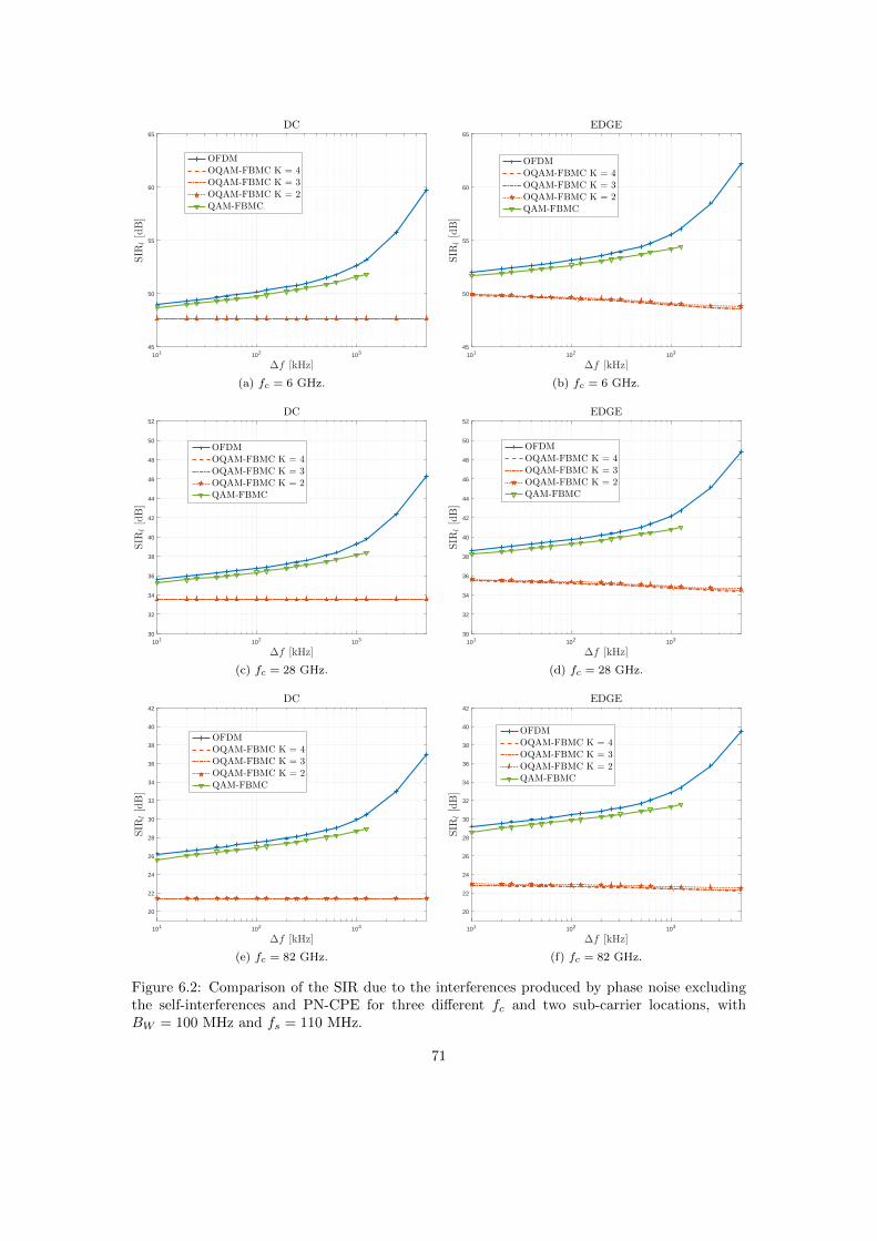
101 102 103

∆f [kHz]

45

50

55

60

65SIR

l[dB]

DC

OFDM

OQAM-FBMC K = 4

OQAM-FBMC K = 3

OQAM-FBMC K = 2

QAM-FBMC

(a) fc = 6 GHz.

101 102 103

∆f [kHz]

45

50

55

60

65

SIR

l[dB]

EDGE

OFDM

OQAM-FBMC K = 4

OQAM-FBMC K = 3

OQAM-FBMC K = 2

QAM-FBMC

(b) fc = 6 GHz.

101 102 103

∆f [kHz]

30

32

34

36

38

40

42

44

46

48

50

52

SIR

l[dB]

DC

OFDM

OQAM-FBMC K = 4

OQAM-FBMC K = 3

OQAM-FBMC K = 2

QAM-FBMC

(c) fc = 28 GHz.

101 102 103

∆f [kHz]

30

32

34

36

38

40

42

44

46

48

50

52

SIR

l[dB]

EDGE

OFDM

OQAM-FBMC K = 4

OQAM-FBMC K = 3

OQAM-FBMC K = 2

QAM-FBMC

(d) fc = 28 GHz.

101 102 103

∆f [kHz]

20

22

24

26

28

30

32

34

36

38

40

42

SIR

l[dB]

DC

OFDM

OQAM-FBMC K = 4

OQAM-FBMC K = 3

OQAM-FBMC K = 2

QAM-FBMC

(e) fc = 82 GHz.

101 102 103

∆f [kHz]

20

22

24

26

28

30

32

34

36

38

40

42

SIR

l[dB]

EDGE

OFDM

OQAM-FBMC K = 4

OQAM-FBMC K = 3

OQAM-FBMC K = 2

QAM-FBMC

(f) fc = 82 GHz.

Figure 6.2: Comparison of the SIR due to the interferences produced by phase noise excludingthe self-interferences and PN-CPE for three different fc and two sub-carrier locations, withBW = 100 MHz and fs = 110 MHz.

71

10 15 20 25 30 35 40 45 50

SNR [dB]

10-6

10-5

10-4

10-3

10-2

10-1

100

SER

OFDM

OFDM, PN-CPE removed

OQAM-FBMC, K=4

(a) fc = 6 GHz and 16-QAM.

10 15 20 25 30 35 40 45 50

SNR [dB]

10-6

10-5

10-4

10-3

10-2

10-1

100

SER

OFDMOFDM, PN-CPE removedOQAM-FBMC, K=4

(b) fc = 6 GHz and 64-QAM.

10 15 20 25 30 35 40 45 50

SNR [dB]

10-6

10-5

10-4

10-3

10-2

10-1

100

SER

OFDM

OFDM, PN-CPE removed

OQAM-FBMC, K=4

(c) fc = 28 GHz and 16-QAM.

10 15 20 25 30 35 40 45 50

SNR [dB]

10-6

10-5

10-4

10-3

10-2

10-1

100

SER

OFDM

OFDM, PN-CPE removed

OQAM-FBMC, K=4

(d) fc = 28 GHz and 64-QAM.

10 15 20 25 30 35 40 45 50

SNR [dB]

10-6

10-5

10-4

10-3

10-2

10-1

100

SER

OFDM

OFDM, PN-CPE removed

OQAM-FBMC, K=4

(e) fc = 82 GHz and 16-QAM.

10 15 20 25 30 35 40 45 50

SNR [dB]

10-6

10-5

10-4

10-3

10-2

10-1

100

SER

OFDMOFDM, PN-CPE removedOQAM-FBMC, K=4

(f) fc = 82 GHz and 64-QAM.

Figure 6.3: Simulation results for the SER due to phase noise, self-interferences and AWGN forthe parameters in Table 6.1.

72

Chapter 7

Conclusions and future work

7.1 Conclusions

In this thesis we have derived the weighting functions for OFDM, QAM-FBMC and OQAM-FDMC, three of the most promising waveform candidates for 5G. The weighting functions allowus to evaluate the effects of phase noise in the performance of the different waveforms in a veryintuitive way. Thus, the derived weighting functions have been used together with the mmMagicphase noise model to obtain different results for the achievable SIR of OFDM, QAM-FBMC andOQAM-FBMC subject to phase noise. Also, Monte Carlo evaluations have been done to verifythe accuracy of the results obtained with the weighting functions. Moreover, the effects of phasenoise in the Symbol Error Rate have been obtained by simulation for OFDM and OQAM-FBMCwith K = 4. Finally, the results for all the waveforms have been compared.

After analysing the results obtained in this thesis, we can conclude that phase noise is only asignificant degradation for very high frequencies in the millimetre-wave bands. We have shownthat QAM-FBMC offers good sensitivity against phase noise (with values quite similar to theOFDM ones). However, it is a non-orthogonal MCM highly degraded by its self-interferences andit offers very poor performance (even without the effect of phase noise). In addition, OQAM-FBMC is a non-orthogonal MCM with worst sensitivity against phase noise than QAM-FBMCbut it is less degraded by its self-interferences, leading to a better performance than QAM-FBMCfor the mmMagic phase noise model. It is important to highlight that the performance of OQAM-FBMC is related with the selected overlapping factor. The sensitivity against phase noise is verysimilar for different overlapping factors, but the power of the self-interferences is different foreach one. It has been shown that OQAM-FBMC with K = 4 outperforms the cases with K = 2and K = 3. Finally, OFDM is an orthogonal MCM and it is not affected by self-interferences.Moreover, it has been shown that its sensitivity against phase noise is very good, mainly becausethe PN-CPE can be easily removed using pilot symbols (without increasing the complexity of thesystem). Thus, OFDM offers a very good performance in the presence of phase noise. We haveexposed that for 64-QAM and 82 GHz the error-floor in the case of OFDM with CPE correctionis lower than 10−5, but in the case of OQAM-FBMC with K = 4 it is higher than 10−2 (for themmMagic phase noise model). After the analysis of all the results, we can conclude that OFDMoutperforms OQAM-FBMC and QAM-FBMC in terms of phase noise effects (for the mmMagicphase noise model) but OQAM-FBMC and QAM-FBMC offer higher spectral density.

73

7.2 Future work

The study presented in this thesis might be continued by extending the comparison of theeffects of phase noise to other waveforms, using similar derivations to the ones presented inChapter 3, 4 and 5. Concretely it might be suitable to derive tools to study the effect of phasenoise in Window-OFDM and DFTS-OFDM (promising waveforms for 5G). It would be alsointeresting to study the shape of the filters used by the different waveforms and how to optimizethem to be more robust against phase noise. Also, the study and analysis of different phasenoise correction methods may be interesting (not only for the PN-CPE, but also for PN-ICI andPN-ISI). Finally, particularly interesting might be to study the probability distribution functionof the interference terms produced by phase noise in order to obtain a method to theoreticallyevaluate the Symbol Error Rate, since the Gaussian assumption is not accurate in this case.

74

Appendices

75

Appendix A

OFDM Derivations

A.1 Derivation of E[|ϕi,l|2

]

In this appendix an expression for E[|ϕi,l|2

]is derived. First, we are going to define a new

filter that will simplify the following derivations

hi,l(t) := pi(t) pl(t) = p2(t) ej2πi−lT t , (A.1)

in which the definition in (2.8) has been used.

Next, the derivation of E[|ϕi,l|2

]follows.

E[|ϕi,l|2

](a)= E

[∣∣∣∣j∫ +∞

−∞φ(τ) pi(τ) pl(τ) dτ

∣∣∣∣2]

(b)= E

[∣∣∣∣j∫ +∞

−∞φ(τ) hi,l(τ) dτ

∣∣∣∣2]

(c)= E

[∫ +∞

−∞

∫ +∞

−∞φ(τ) hi,l(τ) φ(τ + t) hi,l(τ + t) dτ dt

]

=

∫ +∞

−∞

∫ +∞

−∞E[φ(τ)φ(τ + t)

]hi,l(τ) hi,l(τ + t) dτ dt

(d)=

∫ +∞

−∞Rφ(−t)

(∫ +∞

−∞hi,l(τ) hi,l(τ + t) dτ

)dt

(e)=

∫ +∞

−∞Rφ(−t)

(hi,l(t) ∗ hi,l(−t)

)dt

(f)=

∫ +∞

−∞

(∫ +∞

−∞Sφ(f)e−j2πtf df

)(hi,l(t) ∗ hi,l(−t)

)dt

=

∫ +∞

−∞Sφ(f)

(∫ +∞

−∞

(hi,l(t) ∗ hi,l(−t)

)e−j2πtf dt

)df

(g)=

∫ +∞

−∞Sφ(f) Wi,l(f) df (A.2)

76

(a) follows from the definition of ϕi,l in (3.6); (b) follows from (A.1); (c) follows from the appli-

cation of the absolute value operator (| |2); (d) follows from the definition of the autocorrelationof a stochastic process, i.e., RX(t) = E [X(τ)X(τ − t)] (being X an stochastic process); (e)follows from the definition of the convolution (∗ is the convolution operator); (f) follows fromthe definition of the autocorrelation of a WSS sthocastic process as the Fourier transform of itsPSD (Sφ(f) is the PSD of phase noise, which is a WSS stochastic process); (g) follows from the

definition of a new function Wi,l(f), which is defined in (A.6).

What follows next is the definition and simplification of Wi,l(f)

Wi,l(f) : =

∫ +∞

−∞

(hi,l(t) ∗ hi,l(−t)

)e−j2πtf dt

(a)= F

hi,l(t) ∗ hi,l(−t)

(b)= F

hi,l(t)

Fhi,l(−t)

(c)= F

hi,l(t)

Fhi,l(t)

(d)=∣∣∣Fhi,l(t)

∣∣∣2

(e)=∣∣∣Fp2(t) ej2π

i−lT t∣∣∣

2

(f)=

∣∣∣∣Fp2(t)

∗ δ(f − i− l

T

)∣∣∣∣2

(g)=

∣∣∣∣sinc(fT ) ∗ δ(f − i− l

T

)∣∣∣∣2

=

∣∣∣∣sinc

((f − i− l

T

)T

)∣∣∣∣2

(A.3)

(a) follows from the definition of the continuous Fourier transform (denoted by the operatorF ); (b) follows from the convolution theorem; (c) follows from the complex conjugate sym-

metry of the real signals and X denotes complex conjugate of X (hi,l(t) is a real-valued signal);

(d) follows from the definition of absolute value; (e) follows from the definition of hi,l(t) in (A.1);(f) follows from the convolution theorem [18, pp. 297]; (g) follows from the Fourier transformof p2(t) (which is a rectangular pulse of amplitude and duration T ).

77

A.2 Derivation of E[|ϕi,l|2

]

In this appendix an expression for E[|ϕi,l|2

]is derived. First, we are going to define a new

filter that will simplify the following derivations

hi,l[n] := pi[n] pl[n] = p2[n] ej2πi−lN n , (A.4)

in which the definition in (3.22) has been used.

Next, the derivation of E[|ϕi,l|2

]follows

E[|ϕi,l|2

](a)= E

∣∣∣∣∣j

+∞∑

s=−∞φ[s] pi[s] pl[s]

∣∣∣∣∣

2

(b)= E

∣∣∣∣∣j

+∞∑

s=−∞φ[s] hi,l[s]

∣∣∣∣∣

2

(c)= E

[+∞∑

n=−∞

+∞∑

s−∞φ[s] hi,l[s] φ[s+ n] hi,l[s+ n]

]

=

+∞∑

n=−∞

+∞∑

s−∞E [φ[s]φ[s+ n]] hi,l[s] hi,l[s+ n]

(d)=

+∞∑

n=−∞Rφ[−n]

(+∞∑

s=−∞hi,l[s] hi,l[s+ n]

)

(e)=

+∞∑

n=−∞Rφ[−n]

(hi,l[n] ∗ hi,l[−n]

)

(f)=

+∞∑

n=−∞

(∫ +0.5

−0.5

Sφ(ν)e−j2πνn dν

)(hi,l[n] ∗ hi,l[−n]

)

=

∫ +0.5

−0.5

Sφ(ν)

(+∞∑

n=−∞

(hi,l[n] ∗ hi,l[−n]

)e−j2πνn

)dν

(g)=

∫ +0.5

−0.5

Sφ(ν)Wi,l(ν) dν (A.5)

(a) follows from (3.30); (b) follows from (A.4); (c) follows from the definition of the absolutevalue; (d) follows from the definition of the autocorrelation of a discrete stochastic process,i.e., RX [n] = E [X[s]X[s− n]] (being X a discrete stochastic process); (e) follows from thedefinition of the convolution (∗ is the convolution operator); (f) follows from the definition ofthe autocorrelation of a discrete WSS sthocastic process as the Inverse Discrete Time FourierTransform (IDTFT) of its PSD (Sφ(ν) is the PSD of sampled phase noise, which is a WSSdiscrete stochastic process); (g) follows from the definition of a new function Wi,l(ν).

78

What follows next is the definition and simplification of Wi,l(ν)

Wi,l(ν) : =

+∞∑

n=−∞

(hi,l[n] ∗ hi,l[−n]

)e−j2πνn

(a)= F hi,l[n] ∗ hi,l[−n](b)= F hi,l[n]F hi,l[−n](c)= F hi,l[n])F hi,l[n](d)= |F hi,l[n]|2

(e)=∣∣∣Fp2[n] ej2π

i−lN n∣∣∣

2

(f)=

∣∣∣∣Fp2[n]

~ δ

(ν − i− l

N

)∣∣∣∣2

(g)=

∣∣∣∣(

1

N

sin (πνN)

sin(πν)eπν(N−1)

)~ δ

(ν − i− l

N

)∣∣∣∣2

=1

N2

∣∣∣∣∣sin(π(ν − i−l

N

)N)

sin(π(ν − i−l

N

))∣∣∣∣∣

2

(A.6)

(a) follows from the definition of the DTFT (denoted by the operator F ); (b) follows fromthe convolution theorem [18, pp. 297]; (c) follows from the complex conjugate symmetry of thereal signals and X denotes complex conjugate of X (hi,l[N ] is a real-valued signal); (d) followsfrom the definition of absolute value; (e) follows from the definition of hi,l[n] in (A.4); (f) followsfrom the convolution theorem (~ is the operator for the circular convolution); (g) follows fromthe DTFT of p2[n] (which is a discrete rectangular pulse with N samples and amplitude N).

Wi,l(ν) : =∣∣∣Fp[n] ej2π

i−lN n∣∣∣

2

=1

N2

∣∣∣∣∣sin(π(ν − i−l

N

)N)

sin(π(ν − i−l

N

))∣∣∣∣∣

2

(A.7)

79

Appendix B

QAM-FBMC Derivations

B.1 Derivation of |λi,l,d|2

In this appendix an expression for |λi,l,d|2 is derived. First, we are going to define a new filterthat will simplify the following derivations

hi,l,d[n] := pi[n− dN ] pl[n] (B.1)

The derivation of |λi,l,d|2 follows.

|λi,l,d|2(a)=

∣∣∣∣∣∞∑

s=−∞pi[s− dN ] pl[s]

∣∣∣∣∣

2

(b)=

∣∣∣∣∣∞∑

s=−∞hi,l,d[s]

∣∣∣∣∣

2

(c)=

∞∑

n=−∞

∞∑

s=−∞hi,l,d[s] hi,l,d[s+ n]

(d)=

∞∑

n=−∞(hi,l,d[n] ∗ hi,l,d[−n])

(e)= F hi,l,d[n] ∗ hi,l,d[−n] (ν = 0)

(f)= Wi,l,d(ν) δ(ν) (B.2)

(a) follows from (4.7); (b) follows from (B.1); (c) follows from definition of the absolute value

(whose operator is | |2); (d) follows from convolution’s definition (whose operator is ∗); (e) fol-lows from the interpretation of the infinite sum as a DTFT in ν = 0 (where ν := f

fsand

F is the DTFT operator); (f) follows from the definition of a new function Wi,l,d(ν) :=F hi,l,d[n] ∗ hi,l,d[−n].

80

What follows next is the definition and simplification of Wi,l,d(ν)

Wi,l,d(ν) : = F hi,l,d[n] ∗ hi,l,d[−n](a)= F hi,l,d[n] F hi,l,d[−n](b)= F hi,l,d[n] F hi,l,d[n](c)= |F hi,l,d[n]|2

(d)=∣∣∣Fpi[n− dN ] pl[n]

∣∣∣2

(e)=∣∣∣F pi[n− dN ]~ F

pl[n]

∣∣∣2

(f)=∣∣∣F pi[n] e−j2πνdN ~ F

pl[n]

∣∣∣2

(g)=∣∣∣Pi(ν) e−j2πνdN ~ Pl(ν)

∣∣∣2

(B.3)

(a) follows from the convolution theorem; (b) follows from the complex conjugate symmetry of theDTFT for a real signal; (c) follows from the definition of absolute value; (d) follows from (B.1);(e) follows from the convolution theorem (where ~ is the circular convolution operator) [18,pp. 297]; (f) follows from the DTFT of a time shift [18, pp. 296]; (g) follows from definingPi(ν) = F pi[n] (ν).

Next, a detailed expression for Pi(ν) is given

Pi(ν) = F pi[n] (ν)(a)=

Fpeven[n] ej2π

iN n

(ν) = Peven(ν − i

N

)if i even

Fpodd[n] ej2π

iN n

(ν) = Podd(ν − i

N

)if i odd

(B.4)

where the frequency shift property of the DTFT has been applied [18, pp. 300]. Also, we definePeven(ν) := F peven[n] and Podd(ν) := F podd[n].

81

B.2 Derivation of E[|βi,l,d|2

]

In this appendix an expression for E[|βi,l,d|2

]is derived. The derivation follows.

E[|βi,l,d|2

](a)= E

∣∣∣∣∣j

+∞∑

s=−∞φ[s] pi[s− dN ] pl[s]

∣∣∣∣∣

2

(b)= E

∣∣∣∣∣j

+∞∑

s=−∞φ[s] hi,l,d[s]

∣∣∣∣∣

2

(c)= E

[+∞∑

n=−∞

+∞∑

s−∞φ[s] hi,l,d[s] φ[s+ n] hi,l,d[s+ n]

]

=

+∞∑

n=−∞

+∞∑

s−∞E [φ[s]φ[s+ n]] hi,l,d[s] hi,l,d[s+ n]

(d)=

+∞∑

n=−∞Rφ[−n]

(+∞∑

s=−∞hi,l,d[s] hi,l,d[s+ n]

)

(e)=

+∞∑

n=−∞Rφ[−n]

(hi,l,d[n] ∗ hi,l,d[−n]

)

(f)=

+∞∑

n=−∞

(∫ +0.5

−0.5

Sφ(ν)e−j2πνn dν

)(hi,l,d[n] ∗ hi,l,d[−n]

)

=

∫ +0.5

−0.5

Sφ(ν)

(+∞∑

n=−∞

(hi,l,d[n] ∗ hi,l,d[−n]

)e−j2πνn

)dν

(g)=

∫ +0.5

−0.5

Sφ(ν)F hi,l,d[n] ∗ hi,l,d[−n] dν

(h)=

∫ +0.5

−0.5

Sφ(ν)Wi,l,d(ν) dν (B.5)

(a) follows from (4.9); (b) follows from (B.1); (c) follows from the definition of the absolutevalue; (d) follows from the definition of the autocorrelation of a discrete stochastic process,i.e., RX [n] = E [X[s]X[s− n]] (being X a discrete stochastic process); (e) follows from thedefinition of the convolution (∗ is the convolution operator); (f) follows from the definition ofthe autocorrelation of a discrete WSS sthocastic process as the IDTFT of its PSD (Sφ(ν) is thePSD of sampled phase noise, which is a WSS discrete stochastic process); (g) follows from thedefinition of Wi,l(ν) := F hi,l,d[n] ∗ hi,l,d[−n] previously derived in (B.3).

82

Appendix C

OQAM-FBMC Derivations

C.1 Derivation of |γi,l,d|2

In this appendix an expression for |λi,l,d|2 is derived. First, we are going to define a new filterthat will simplify the following derivations

hRi,l,d[n] : = <θi,d pi

[n− dN

2

]θl pl[n]

(a)= <

ji−l+d p[n] p

[n− dN

2

]ej2π

i−lN n

(b)= <

p[n] p

[n− dN

2

]ej(2π i−lN n+(i−l+d)π2 )

(c)= p[n] p

[n− dN

2

]<

ejΩi,l,d[n]

(d)= p[n] p

[n− dN

2

]cos(Ωi,l,d[n]) (C.1)

(a) follows from θi,d θl = ji−l+d and from (5.2); (b) follows from ji−l+d = ej(i−l+d)π2 ; (c) followsby defining Ωi,l,d[n] := 2π i−lN n+ (i− l + d)π2 and takes into account that p[n] ∈ R, ∀n ∈ R; (d)follows from Euler’s formula, i.e., ejx = cos(x) + j sin(x) ∀x ∈ R.

83

The derivation of |λi,l,d|2 follows

|γi,l,d|2(a)=

∣∣∣∣∣∞∑

s=−∞<θi,d pi

[s− dN

2

]θlpl[s]

∣∣∣∣∣

2

(b)=

∣∣∣∣∣∞∑

s=−∞hRi,l,d[s]

∣∣∣∣∣

2

(c)=

∞∑

n=−∞

∞∑

s=−∞hRi,l,d[s] h

Ri,l,d[s+ n]

(d)=

∞∑

n=−∞

(hRi,l,d[n] ∗ hRi,l,d[−n]

)

(e)= F

hRi,l,d[n] ∗ hRi,l,d[−n]

(ν = 0)

(f)= WS

i,l,d(ν) δ(ν) (C.2)

(a) follows from (5.7); (b) follows from (C.1); (c) follows from definition of the absolute value; (d)follows from convolution’s definition (whose operator is ∗); (e) follows from the interpretationof the infinite sum as a DTFT in ν = 0 (where ν := f

fsand F is the DTFT operator); (f)

follows by defining WSi,l,d(ν) := F

hRi,l,d[n] ∗ hRi,l,d[−n]

which is derived in (C.3).

What follows next is the definition and simplification of WSi,l,d(ν)

WSi,l,d(ν) : = F

hRi,l,d[n] ∗ hRi,l,d[−n]

(a)= F

hRi,l,d[n]

FhRi,l,d[−n]

(b)= F

hRi,l,d[n]

FhRi,l,d[n]

(c)=∣∣FhRi,l,d[n]

∣∣2

(d)=

∣∣∣∣Fp[n] p

[n− dN

2

]cos(Ωi,l,d[n])

∣∣∣∣2

(e)=

∣∣∣∣Fp[n] p

[n− dN

2

]~ F cos(Ωi,l,d[n])

∣∣∣∣2

(f)=

∣∣∣∣Vd(ν) ~ F

cos

(2πi− lN

n+ (i− l + d)π

2

)∣∣∣∣2

(g)=

∣∣∣∣∣Vd(ν) ~

(δ(ν − i−l

N

)ej(i−l+d)π2 + δ

(ν + i−l

N

)e−j(i−l+d)π2

2

)∣∣∣∣∣

2

(h)=

∣∣∣∣∣Vd(ν − i−l

N

)ej(i−l+d)π2 + Vd

(ν + i−l

N

)e−j(i−l+d)π2

2

∣∣∣∣∣

2

(i)=

1

4

[∣∣∣∣Vd(ν − i− l

N

)∣∣∣∣2

+

∣∣∣∣Vd(ν +

i− lN

)∣∣∣∣2

+ 2 <Yi,l,d(ν)]

(C.3)

84

(a) follows from the convolution theorem [18, pp. 297]; (b) follows from the complex conjugatesymmetry of the DTFT for a real signal; (c) follows from the definition of absolute value; (d)follows from (C.1); (e) follows from the convolution theorem (where ~ is the circular convolution

operator); (f) follows by defining Vd(ν) := Fp[n] p

[n− dN2

]= P (ν)~

(P (ν)e−2πν N2 d

), being

P (ν) := F p[n]; (g) follows from the DTFT of a cosine; (h) follows from the application of thecircular convolution operator; (i) follows from the application of the absolute value operator andYi,l,d(ν) is defined as

Yi,l,d(ν) := ejπ(i−l+d)Vd

(ν − i− l

N

)V ∗d

(ν +

i− l

N

)

85

C.2 Derivation of E[|ρi,l,d|2

]

In this appendix an expression for E [|ρi,l,d|]2 is derived. First, we are going to define a newfilter that will simplify the following derivations

hIi,l,d[n] : = <j θi,d pi

[n− dN

2

]θl pl[n]

(a)= <

j ji−l+d p[n] p

[n− dN

2

]ej2π

i−lN n

(b)= <

j p[n] p

[n− dN

2

]ej(2π i−lN n+(i−l+d)π2 )

(c)= p[n] p

[n− dN

2

]<j ejΩi,l,d[n]

(d)= −p[n] p

[n− dN

2

]sin(Ωi,l,d[n]) (C.4)

(a) follows from θi,d θl = ji−l+d and from (5.2); (b) follows from ji−l+d = ej(i−l+d)π2 ; (c) followsby defining Ωi,l,d[n] := 2π i−lN n+ (i− l + d)π2 and takes into account that p[n] ∈ R, ∀n ∈ R; (d)follows from Euler’s formula, i.e., ejx = cos(x) + j sin(x) ∀x ∈ R.

86

Next, the derivation of a suitable expression for E[|ρi,l,d|2

]follows.

E[|ρi,l,d|2

](a)= E

∣∣∣∣∣j

+∞∑

s=−∞<j φ[s] θi,d pi

[s− dN

2

]θl pl[s]

∣∣∣∣∣

2

(b)= E

∣∣∣∣∣j

+∞∑

s=−∞φ[s] hIi,l,d[s]

∣∣∣∣∣

2

(c)= E

[+∞∑

n=−∞

+∞∑

s−∞φ[s] hIi,l,d[s] φ[s+ n] hIi,l,d[s+ n]

]

=

+∞∑

n=−∞

+∞∑

s−∞E [φ[s]φ[s+ n]] hIi,l,d[s] h

Ii,l,d[s+ n]

(d)=

+∞∑

n=−∞Rφ[−n]

(+∞∑

s=−∞hIi,l,d[s] h

Ii,l,d[s+ n]

)

(e)=

+∞∑

n=−∞Rφ[−n]

(hIi,l,d[n] ∗ hIi,l,d[−n]

)

(f)=

+∞∑

n=−∞

(∫ +0.5

−0.5

Sφ(ν)e−j2πνn dν

)(hIi,l,d[n] ∗ hIi,l,d[−n]

)

=

∫ +0.5

−0.5

Sφ(ν)

(+∞∑

n=−∞

(hIi,l,d[n] ∗ hIi,l,d[−n]

)e−j2πνn

)dν

(g)=

∫ +0.5

−0.5

Sφ(ν)FhIi,l,d[n] ∗ hIi,l,d[−n]

dν

(h)=

∫ +0.5

−0.5

Sφ(ν)Wi,l(ν) dν (C.5)

(a) follows from (5.8); (b) follows from (C.4); (c) follows from the definition of the absolutevalue; (d) follows from the definition of the autocorrelation of a discrete stochastic process,i.e., RX [n] = E [X[s]X[s− n]] (being X a discrete stochastic process); (e) follows from thedefinition of the convolution (∗ is the convolution operator); (f) follows from the definition ofthe autocorrelation of a discrete WSS sthocastic process as the IDTFT of its PSD (Sφ(ν) is thePSD of sampled phase noise, which is a WSS discrete stochastic process); (g) follows by defining

Wi,l(ν) := FhIi,l,d[n] ∗ hIi,l,d[−n]

, which is derived next in (C.6).

87

What follows next is the definition and simplification of Wi,l,d(ν)

Wi,l,d(ν) : = FhIi,l,d[n] ∗ hIi,l,d[−n]

(a)= F

hIi,l,d[n]

FhIi,l,d[−n]

(b)= F

hIi,l,d[n]

FhIi,l,d[n]

(c)=∣∣FhIi,l,d[n]

∣∣2

(d)=

∣∣∣∣Fp[n] p

[n− dN

2

]sin(Ωi,l,d[n])

∣∣∣∣2

(e)=

∣∣∣∣Fp[n] p

[n− dN

2

]~ F sin(Ωi,l,d[n])

∣∣∣∣2

(f)=

∣∣∣∣Vd(ν) ~ F

sin

(2πi− lN

n+ (i− l + d)π

2

)∣∣∣∣2

(g)=

∣∣∣∣∣Vd(ν) ~

(δ(ν − i−l

N

)ej(i−l+d)π2 − δ

(ν + i−l

N

)e−j(i−l+d)π2

2j

)∣∣∣∣∣

2

(h)=

∣∣∣∣∣Vd(ν − i−l

N

)ej(i−l+d)π2 − Vd

(ν + i−l

N

)e−j(i−l+d)π2

2j

∣∣∣∣∣

2

(i)=

1

4

[∣∣∣∣Vd(ν − i− l

N

)∣∣∣∣2

+

∣∣∣∣Vd(ν +

i− lN

)∣∣∣∣2

− 2 <Yi,l,d(ν)]

(C.6)

(a) follows from the convolution theorem [18, pp. 297]; (b) follows from the complex conjugatesymmetry of the DTFT for a real signal; (c) follows from the definition of absolute value; (d)follows from (C.4); (e) follows from the convolution theorem (where ~ is the circular convolution

operator); (f) follows by defining Vd(ν) := Fp[n] p

[n− dN2

]= P (ν)~

(P (ν)e−2πν N2 d

), being

P (ν) := F p[n]; (g) follows from the DTFT of a sine; (h) follows from the application of thecircular convolution operator; (i) follows from the application of the absolute value operator andYi,l,d(ν) is defined as

Yi,l,d(ν) := ejπ(i−l+d)Vd

(ν − i− l

N

)V ∗d

(ν +

i− l

N

)

88

Bibliography

[1] J. Luo, A. A. Zaidi, J. Vihriala, D. Giustiniano, Y. Qi, H. Halbauer, D. Ktnas, R. Weiler,H. Miao, and J. Lorca, “Millimetre-Wave Air-Interface for 5G: Challenges and design prin-ciples,” in ETSI Workshop on future radio technologies - Air interfaces, January 2016.

[2] J. Luo, A. A. Zaidi, J. Vihriala, and D. Giustiniano, “Preliminary radio interface concepts formm-wave mobile communications,” tech. rep., Millimetre-Wave Based Mobile Radio AccessNetwork for Fifth Generation Integrated Communications (mmMAGIC), Deliverable D4.1,June 2016. [Online]. Available: https://5g-mmmagic.eu/results. Accessed: 2016-09-11.

[3] J. Stott, “The effects of phase noise in COFDM,” tech. rep., BBC Research and Devel-opment, July 1998. [Online]. Available: https://tech.ebu.ch/docs/techreview/trev_

276-stott.pdf. Accessed: 2016-09-11.

[4] L. Piazzo and P. Mandarini, “Analysis of phase noise effects in OFDM modems,” IEEETransactions on Communications, vol. 50, pp. 1696–1705, Oct 2002.

[5] A. Ishaque and G. Ascheid, “On the sensitivity of SMT systems to oscillator phase noiseover doubly-selective channels,” in 2015 IEEE Wireless Communications and NetworkingConference (WCNC), pp. 545–550, March 2015.

[6] S. Hara and R. Prasad, Multicarrier techniques for 4G mobile communications. ArtechHouse, 2003.

[7] G. Turin, “An introduction to matched filters,” IRE Transactions on Information Theory,vol. 6, pp. 311–329, June 1960.

[8] K. Grchenig, Foundations of Time-Frequency Analysis. Springer, 1st ed., 2001.

[9] H. Nam, M. Choi, C. Kim, D. Hong, and S. Choi, “A new filter-bank multicarrier systemfor QAM signal transmission and reception,” in 2014 IEEE International Conference onCommunications (ICC), pp. 5227–5232, June 2014.

[10] M. Bellanger, “FBMC physical layer: a primer,” tech. rep., PHYDYAS PHYsical layer forDYnamic AccesS and cognitive radio, 2010. [Online]. Available: http://www.ict-phydyas.org/teamspace/internal-folder/FBMC-Primer_06-2010.pdf. Accessed: 2016-09-11.

[11] J. Louveaux, L. Baltar, and D. Waldhauser, “D3.1 - Equalization and demodulation inthe receiver (single antenna),” tech. rep., PHYDYAS PHYsical layer for DYnamic Ac-cesS and cognitive radio, July 2008. [Online]. Available: http://www.ict-phydyas.org/

delivrables/PHYDYAS-D3.1.pdf/at_download/file. Accessed: 2016-09-11.

89

[12] A. Mehrotra, “Noise analysis of phase-locked loops,” IEEE Transactions on Circuits andSystems I: Fundamental Theory and Applications, vol. 49, pp. 1309–1316, Sep 2002.

[13] “mmMAGIC (Millimetre-Wave Based Mobile Radio Access Network for Fifth GenerationIntegrated Communications).” https://5g-mmmagic.eu/. Accessed: 2016-09-11.

[14] S. Wu and Y. Bar-Ness, “A phase noise suppression algorithm for OFDM-based WLANs,”IEEE Communications Letters, vol. 6, pp. 535–537, Dec 2002.

[15] J. Vihril, A. A. Zaidi, V. Venkatasubramanian, N. He, E. Tiirola, J. Medbo, E. Lhetkan-gas, K. Werner, K. Pajukoski, A. Cedergren, and R. Baldemair, “Numerology and framestructure for 5G radio access,” in 27th annula IEEE international symposium on personal,indoor and mobile radio communications, September 2016.

[16] T. C. W. Schenk, R. W. V. D. Hofstad, E. R. Fledderus, and P. F. M. Smulders, “Distri-bution of the ICI term in phase noise impaired OFDM systems,” IEEE Transactions onWireless Communications, vol. 6, pp. 1488–1500, April 2007.

[17] Y. H. Yun, C. Kim, K. Kim, Z. Ho, B. Lee, and J. Y. Seol, “A new waveform enablingenhanced QAM-FBMC systems,” in 2015 IEEE 16th International Workshop on SignalProcessing Advances in Wireless Communications (SPAWC), pp. 116–120, June 2015.

[18] J. Proakis and D. Manolakis, Digital Signal Processing: Principles, Algorithms and Appli-cations. Prentice-Hall Internacional, Inc, 3rd ed., 1996.

90

TRITA TRITA-EE 2016:176

ISSN 1653-5146

www.kth.se