a comparative study with flow visualization of turbulent fluid - ijest

Rabin Debnath et. al. / International Journal of Engineering Science and Technology Vol. 2(9), 2010, 4108-4121

A COMPARATIVE STUDY WITH FLOW VISUALIZATION OF TURBULENT

FLUID FLOW IN AN ELBOW

RABIN DEBNATH* Research scholar, Department of Mechanical Engineering, Jadavpur University

Kolkata- 700 032, West Bengal, India

SOMNATH BHATTACHARJEE Research scholar, Department of Mechanical Engineering, Jadavpur University


ARINDAM MANDAL Research Scholar, Department of Mechanical Engineering, Jadavpur University


DEBASISH ROY Reader, Department of Mechanical Engineering, Jadavpur University, Kolkata


SNEHAMOY MAJUMDER Reader, Department of Mechanical Engineering, Jadavpur University, Kolkata


Abstract The analysis of the turbulent fluid flow in an elbow is important for a wide range of engineering

applications like heat exchangers, particle transport piping system, air conditioning devices, pneumatic conveying system etc. Elbow is an important component of pneumatic conveying system and the flow structure within it plays an important role to covey materials. In this paper, a comparative study has been made between three types of turbulent models e.g. standard -ε, -ω and Reynolds Stress models with flow visualization for the turbulent air flow in a two-dimensional rectangular elbow. The possible existence of re-circulation generated in the bent portions of elbow has also been investigated numerically with proper attention of estimating their sizes and strengths. Key words: Rectangular Elbow, -ε model, -ω model, Reynolds Stress model, Recirculation zone 1. Introduction

The analysis of the fluid flow in an elbow is important for a number of engineering applications like heat exchangers, particle transport piping system, air conditioning devices etc. The study of the incompressible, Newtonian turbulent flow through a two-dimensional rectangular elbow is the principal interest of this paper. In this paper, a numerical comparative study has been carried out between three types turbulent models i.e. standard -ε, -ω and Reynolds transport theorem with flow visualization for the turbulent air flow in a two-dimensional rectangular elbow. A brief review of past experimental and numerical studies of such flow is being mentioned herewith. In early studies, a turbulent characteristic in a boundary layer with zero pressure gradients is reported by Klebanoff [1]. His result was based on experimental analysis. He gave an idea about the importance of the region near the wall and the local isotropy. Ito and Imai [2] established the pressure losses in vane elbows of circular cross section. Turbulent shear flow in curved duct was investigated by Ellis and Joubert [3]. They compared the result of two curved rectangular flow with a straight duct flow. Mean velocity profiles, turbulence intensity distributions and stream wise energy spectra are presented for turbulent air flow in a smooth-walled was investigated by Hunt and Joubert [4]; they worked in high aspect ratio rectangular duct with small stream wise curvature, and were compared with measurements taken in a similar straight duct. Humphrey et al. [5] investigated the steady, incompressible, isothermal, developing flow in a square-section curved duct with smooth walls. They measured the longitudinal and radial components of mean velocity and corresponding components of the Reynolds stress tensor with a laser-

ISSN: 0975-5462 4108


Doppler anemometer and the secondary mean velocities, driven mainly by the pressure field. Turbulent flow in 90° square duct and pipe bends was numerically computed by Briley et al. [6] with the help of Navier-Stokes equation. In their study, they approached that the numerical solution of the compressible Reynolds averaged Navier-Stokes equations in the low Mach number regime (M = 0.05) for which they approximated the flow of a liquid. The governing equations were solved using an efficient and non-iterative time-dependent linearized block implicit (LBI) scheme. The measurements and calculations for laminar flows through 90-degree rectangular diversions over a range of Reynolds numbers, discharge ratios and duct aspect ratios (height-to-width ratio, AR=H : W) were reported by Liepsch et al. [7]. Turbulent flow simulation was reported by Chen and Lian [8]. They carried out two dimensional calculations using a finite difference discretization method in conjunction with the standard high Reynolds number -ε model. Shimomizuki et al. [8] numerically analyzed the particle dynamics in a bend of a rectangular duct using Monte Carlo simulation method. Numerical solution of the incompressible Navier-Stokes equations for steady, laminar flows through 900 diversions of rectangular cross section were given by Neary and Sotiropoulos [9]. Their calculations were carried out for various Reynolds numbers, discharge ratios and duct aspect ratios. They shown that for large aspect ratios ducts, the flow at the symmetry plane is significantly affected by the distant top and bottom solid boundaries. Turbulent flow characteristics in the curved duct with a baffle were predicted by Zhang et al. [10]. They used -ε model to represent the turbulent in normal and curved ducts and numerically and experimentally. They predicted the intensity of the secondary flow in a duct with baffle is reduced compared to duct without baffle. Bergstorm et al. [11] predicted the wall mass transfer rates in turbulent flow through a 900 two dimensional bend numerically. Turbulent flow in a 900 bend of circular cross section was investigated experimentally by Sudo et al. [12]. The behaviors of gas particle flow in a horizontal pipe following a 900 horizontal to vertical elbow were investigated experimentally by Akilli et al. [13]. Their experiments were conducted in a 0.154m ID test section. Experiments were performed with conveying air velocities ranging from 15-30 m/s and air-to-solids mass flow rate ratios of 1 and 3, with elbows having bend radius to pipe diameter ratios of 1.5 and 3 . They observed that the strong rope created by the elbow disintegrated within an axial distance of 10 pipe diameters. Fully developed concentration and velocity profiles were obtained within approximately 30 pipe diameters from the elbow exit plane. The rope behaviors were found different for the two elbows (R/D= 1.5 and 3). The shapes of the fully developed profiles were found to be independent of inlet conditions. A correlation for maximum mass transfer coefficient in elbows based on three dimensional computational flow modeling and mass transfer predictions was developed by Wang and Shirazi [14]. The correlation is a function of the flow Reynolds number, Schmidt number and the elbow radius to diameter (r/D) ratio. The correlation for the maximum mass transfer coefficient in an elbow to the mass transfer coefficient in a fully developed pipe flow (MTCRE) is in a good agreement with the CFD code results that are verified with the available experimental data for flow and mass transfer in elbows. An experimental study of the developing turbulent boundary layers on the concave and convex walls of 900 bend of square cross-section using hot wire anemometry were presented by Mokhtarzadeh-Dehghan and Yuan [15]. The bend has a mean radius to height ratio of R/H=1.17. The Reynolds number of the flow 3.6X105 and at start of the bend the boundary thickness to the radius of the curvatures ratio were found 0.041and 0.054 on the concave and convex walls respectively. Single phase pressure drop for turbulent fluid flow in 900 bend was predicted by Crawford et al. [16]. They only predicted the frictional effects in the existing model but no precise models were found available to predict the flow due to separation. Spedding et al. [17] studied the same topic experimentally. They measured the pressure drop in the curved pipes and elbow bends for both laminar and turbulent single phase fluid flow. They predicted the pressure loss for the curved pipe under laminar flow with empirical relations. The transitional Reynolds number was also predicted from an empirical relation and turbulent flow in the curved pipes of large bends. Pressure loss in two-phase upward flow in 900 bend was given by Azzi and Friedel [18]. Kuan [19] predicted the performance of dilute gas-solid flow through a curved 900 duct bend. The curved duct is square sectioned and has a turning radius of 1.5 times the duct’s hydraulic diameter. Turbulent flow quantities at Re=15000 were calculated based on differential Reynolds stress model, while solid velocities were predicted by Lagrangian particle tracking model. A numerical investigation for gas-solid flow in a U-bend was given by Hidayat and Rasmuson [20]. They predicted that increasing the number of bend would cause an increase in pressure drop. Yang and Kuan [21] obtained the mean and the turbulent flow velocities of gas and particulate phases inside a curved 900 bend. They used 2-D Laser Doppler Anemometry (LDA) for obtaining the mean and fluctuating velocities of gas and particulate phases. They used a duct of square cross-section and with air flow velocity 10m/s. Gas-liquid two-phase turbulent flow simulation was reported by Spedding and Benard [22]. They used 900 elbow bend with 0.026 internal diameter of pipe. Their study presented a general correlation for the elbow bend pressure drop in terms of total Reynolds number. A modified Lockhart-Martinelli model was used to predict the result-data. Kim et al. [23] had shown clearly the characteristic geometric effects of 90-degree elbow in the transport of one-dimensional interfacial area concentration and void fraction along the flow. Their study investigated the geometric

ISSN: 0975-5462 4109


effects of flow obstruction on the distribution of local two-phase flow parameters and their transport characteristics in horizontal bubbly flow. A numerical investigation into the physical characteristics of the dilute gas-particle flow over a square cross-sectioned 900 bend was reported by Mohanarangam et al. [24]. In their study, modified Eulerian two-fluid model was employed for the gas-particle flow. Debnath et al. [25] analysed experimentally the turbulent air flow in a two-dimensional rectangular elbow at high Reynolds numbers. They investigated the velocity profiles, flow separation, re-circulation and friction drag etc. in detail. In their study, the effects of Reynolds numbers on the variable discharge of the blower coupled with inlet of the elbow and the possible existence of the recirculation zones generated in the flow region had also been investigated. Experimental investigation of air-water two-phase flow pressure drop in vertical internally wavy 900 bend had been carried out by Benbella et al. [26]. The confined central and annular jet flow through a two-dimensional elbow was reported by Debnath et al. [27]. Their numerical study includes the steady, laminar and incompressible Newtonian fluid flow through a two-dimensional elbow. The CONTROL VOLUME formulation with SIMPLER Algorithm having POWER law scheme was employed to obtain velocity profiles along with visualization of the possible existence of the re-circulation generated due to jet flow as well as sudden change in geometry. El-Gammal et al. [28] investigated the hydrodynamic effect of single phase flow on flow accelerated corrosion in a 900 elbow at a Reynolds number of 40,000. Mandal et al. [29] presented an experimental analysis of the turbulent air flow through a rectangular diffuser using baffles. A rough correlation had been formulated to estimate the recirculation size within the permissible limit of the size of the baffles they had opted. The same authors [30] further investigated the turbulent fluid flow in a rectangular elbow. A rectangular elbow duct of 1.470 m in length with 0.161m hydraulic diameter and working fluid air were used in their experimental study. They investigated the flow visualization and estimation of co-efficient of friction. The velocity profiles along the elbow duct were observed at Reynolds numbers of 3.8X104 and 4.8X104 respectively. Their experimental results had shown that the size of the re-circulation bubble increases with the increase of Reynolds number and the location of the re-circulation bubble around the outer and inner wall of the bend is independent of the Reynolds number. It was also found that the friction factor variation with respect to length along the wall of the elbow duct is quite asymmetric and as a consequence the flow in the downstream side is chaotic and unpredictable. In this paper, a comparative study is made between three types of turbulent models e.g. standard -ε, -ω and Reynolds Stress models with flow visualization of the turbulent fluid flow in an elbow. The purpose of the present work is to observe the detail of the flow behaviors in each of three turbulent models used for a two-dimensional rectangular elbow using air as the working fluid. The detail dimension of the geometry of the flow condition is given in the consecutive paragraph. 2. Geometrical Description: The geometry is two-dimensional rectangular elbow with lengths L1=10m, L2=15m, L3=20m and width W=5m, as essentially shown in the figure 1. The fluid used is the air of density =1.225kg/m3 and

viscosityl=1.85310-5N /m-s.

ISSN: 0975-5462 4110


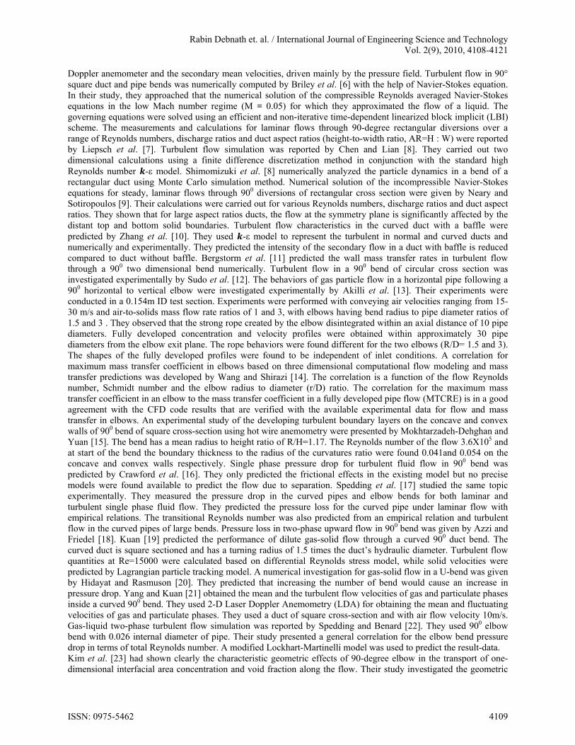
Fig.1. Schematic diagram of the two dimensional rectangular elbow

For the present investigation the following nomenclature has been taken. L1 = 10 m. L2 = 15 m. H = 20 m Width (W) = 5 m. Air density, =1.225 kg/m3.

Molecular viscosity of air, l=1.85310-5N/m-s. Reynolds number, Re = (Umean DH)/l. where Umean is the mass-averaged axial inlet velocity. 3. Mathematical Modeling The three turbulent model equations used for a fluid having constant density ρ, viscosity μ in rectangular Cartesian Co-ordinate system are as follow. 3.1. Governing Equations 3.1.1. Continuity Equation

0 3.1.2. Momentum Equation X- Component:

e

Uin a b

c

d

f g

Distance from Inlet a a X = 4 b b X = 7 e e X = 17 f f X = 20 g g X = 23 Distance from Bottom line of the lower Horizontal limb c c Y = 7 d d Y = 12

X

Y

L1 L2

H

OU

TL

ET

W

a b

c

d

e f g

ISSN: 0975-5462 4111


Y- Component:

3.2. k-ε Model

Transport equations for standard -ε model are given by- 3.2.1. k Equation

3.2.2. ε Equation

Here, kCC ,2,1 and are the empirical turbulence constants, and some typical values of these

constants in the standard model are recommended by Launder and Spalding which are given below-

1C = 1.44 2C = 1.92

k = 1.0

= 1.3

The standard wall function has been adopted from Launder et al. [31] for the solution of the k equations for the problem investigated here. 3.3. -ω model: Transport equations for standard -ω model are given by- 3.3.1. k Equation

3.3.2. ω Equation

Closer coefficient and auxiliary relations

ISSN: 0975-5462 4112


3.4. Reynolds stress model: 3.4.1. u Equation

′ ′ ′ 3.4.2. v Equation

′ ′ ′ 4. Results and Discussions

The Cartesian co-ordinate system has been adopted for computational analysis and solution methodology to solve the governing equations, using Power-Law scheme. Streamline contours, Velocity vector plots and velocity distributions are presented and discussed thoroughly below. The final solutions for all of the subsequent numerical experimentation has been carried out for a uniform grid system 151x151 mesh all along X and Y directions.

In the figures 2-3, 7-8 and 12-13, it has been seen that a simple uniform flow through the inlet of an elbow generating different sizes of re-circulation bubbles residing at near the bent zones of the elbow. From streamline contour flow figures 2 and 12 as well as their corresponding velocity vector as shown in figures 3 and 13, it is obvious that near the corners there are strong recirculation flows which change the configuration of the main flow field. Here, in the lower part of the upper horizontal limb the existence of comparatively large re-circulation bubble is identified. However, at the right and left corner zones of the vertical limb similar re-circulation bubbles are identified in all of the results of ε, and Reynolds stress models respectively. Though the Reynolds stress model lacking one vortex or may be two vortices coalesces to form a larger bubble at that location. In the figures 4, 5 and 6 velocity distribution in the re-circulation bubbles have been shown. From the figure 5 it is obvious that the more we go in the downstream direction the more is the strength of re-circulation bubble. This is also evident from the flow visualization presented in the figures 2 and 3. In the next text we will compare the results with the different models in details. 4.1. Results of k-ε model

Fig.2. Stream Line Contour of k-ε model

ISSN: 0975-5462 4113


Fig.3. Velocity Vector of k-ε model

Fig.4. Velocity Distribution profiles through lower horizontal limb

Fig.5. Velocity Distribution profiles through vertical limb

ISSN: 0975-5462 4114


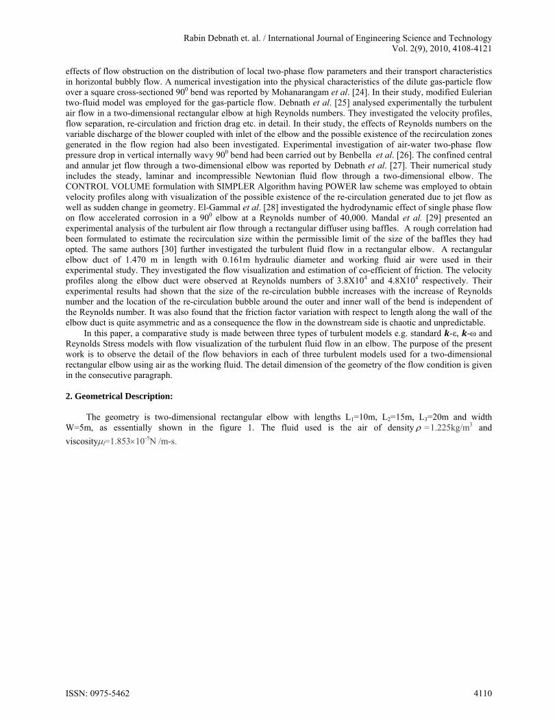
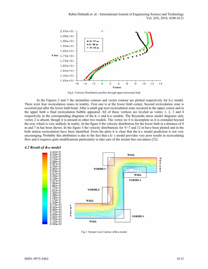
Fig.6. Velocity Distribution profiles through upper horizontal limb

In the Figures 2 and 3 the streamline contour and vector contour are plotted respectively for k- model.

There exist four recirculation zones in totality. First one is at the lower limb corner, Second recirculation zone is occurred just after the lower limb bend. After a small gap next recirculation zone occurred in the upper corner and in the upper limb a final recirculation bubble appeared. All of these vortices are leveled as vortex 1, 2, 3 and 4 respectively in the corresponding diagrams of the k- and k-ω models. The Reynolds stress model diagrams only vortex 2 is absent, though it is present in other two models. The vortex no 4 is incomplete as it is extended beyond the exit, which is very unlikely in reality. In the figure 4 the velocity distribution for the lower limb in a distance of 4 m and 7 m has been shown. In the figure 5 the velocity distributions for Y=7 and 12 m have been plotted and in the both station recirculation have been identified. From the plots it is clear that the k-ε model prediction is not very encouraging. Probably this attribution is due to the fact that a k- ε model provides very poor results in recirculating flow and it requires quite modifications particularly to take care of the stream line curvatures [32]. 4.2 Result of -ω model

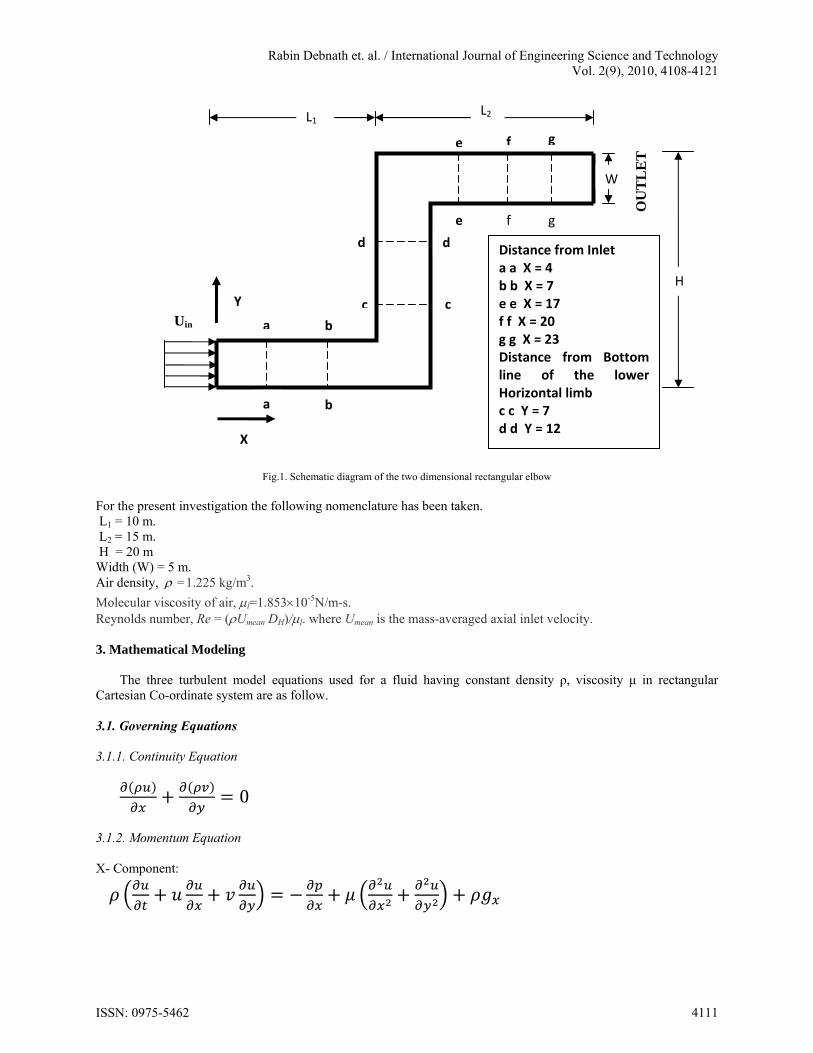
Fig.7. Stream Line Contour of -ω model

ISSN: 0975-5462 4115


Fig.8. Velocity Vector of -ω model

Fig.9. Velocity Distribution profiles through lower horizontal limb

Fig.10. Velocity Distribution profiles through vertical limb

ISSN: 0975-5462 4116


Fig.11. Velocity Distribution profiles through upper horizontal limb

The Figures 7 and 8 exhibit the streamline contour and vector contour respectively for k-ω model. Here

again all of the four recirculation zones have been observed as usual. Here it is noticed that large gap between vortex 2 and vortex 3 exists. The vortex 4 is terminated over within the length of the upper limb. It appears that this position of the vortex at that locality is quite reasonable and physically possible. The velocity distributions are plotted in figure 9 for the lower limb in a distance of 4 m and 7 m respectively and they are quite reasonable meaningful so far as physical significances are concerned. In the figure 10 the velocity distribution for the vertical limb has been plotted and here for both of the stations the recirculations are identified as earlier. These results are physically possible; at least they are reasonable and meaningful so far as physical aspects of flow geometries are concerned. 4.3. Result of Reynolds Stress model

Fig.12. Stream Line Contour of Reynolds Stress model

ISSN: 0975-5462 4117


Fig. 13. Velocity Vector of Reynolds Stress model

Fig. 14. Velocity Distribution profiles through lower horizontal limb

Fig. 15. Velocity Distribution profiles through vertical limb

ISSN: 0975-5462 4118


Fig. 16. Velocity Distribution profiles through upper horizontal limb

In the Figure 12 and 13 the streamline and vector contours are plotted respectively for the Reynolds stress

model. Here we find three recirculation zones, namely vortex 1, 2 and 3 respectively and vortex 2 and vortex 3 are comparatively large and stronger. Vortex 3 is not complete in its life within the upper limb similar to the vortex of the k-ε model. It appears that it is extended beyond the exit, which is similar to the results of k-ε. In the figure 14 we plot the velocity distribution graph for the lower limb in a distance 4 m and 7 m. In the figure 15 we get the velocity distribution for the vertical limb and here for both station we get the recirculation.

Finally we can say that the recirculation bubbles are present in all of the bends as well as at the lower part of the upper limb. However the experimental [30] results are not quite capable of capturing all of them, may be in future by the use of PIV the other recirculation bubbles of micro ranges can be captured better. Comparing all these results we can say that the k-ω equation is providing better option for analyzing the elbow turbulent flow. Actually the k-ω equation predicts better near the wall in contrast to any other turbulent model like the k-ε and other models. Here it is worthy to mention in an elbow lots of bends and walls are encountered and probably that is why the other models are acting poorly in an elbow. 5. Conclusions

A comparative study has been carried out in the Numerical experimentations of turbulent flow through an elbow. It has been observed that all of them predicting the existence of the recirculation bubbles with roughly at the similar geometrical position. However their size and strength were different for the different models. The comparative study reveals that the -ω model predicts better so far as size and physical interpretations are concerned. Among the other two Reynolds stress models predicts little better. This is quite possible from the fact that the k-ε models are poor in capturing the separated flow. The present authors are in this notion that this should be extensively studied using PIV etc. Nomenclature

C [Empirical constant]

tC [Craya- Curtet number]

D H [Hydraulic Dia. of the elbow, m]

f [Friction factor]

G [Production term]

1K , 2K [Constants]

L 1 [Length of the lower horizontal limb, m]

L2 [Length of the upper horizontal limb, m]

H [Height of the elbow, m] W [Width of the elbow, m] u [Time mean velocity along x-axis,

m/s]

inU [Inlet flow velocity, m/s]

meanU

[Mass-averaged mean axial

velocity, m/s] v [Time mean velocity along y-axis,

m/s]

ISSN: 0975-5462 4119


X [Axial co-ordinate along the duct]

Greek Letters [Turbulent dissipation rate, m2/s3]

k [Turbulent kinetic energy, m2/s2]

[Viscosity of the air, kg/m-s]

eff [Effective viscosity, kg/m-s]

l [Laminar viscosity, kg/m-s]

t [Eddy viscosity, kg/m-s]

[Density of air, kg/m3]

Subscripts in [Inlet] l [Laminar] t [Turbulent] eff [Effective]

Re [Reynolds Number,vD

]

[Stream function, m2/s]

6. References [1] Klebanoff, P. S., 1954, “Characteristics of turbulence in a boundary layer with zero pressure gradient” NACA TN 3178. [2] Ito, H. and Imai, K., 1966, “Pressure losses in vaned elbows of a circular cross section”, Transactions of the ASME, Series D, pp. 684-685. [3] Ellis, L.B. and Joubert, P.N., 1974, “Turbulent shear flow in a curved duct”, J. Fluid Mech.62, pp.65-84. [4] Hunt, I. A. and Joubert, P. N.,1979, “Effects of small streamline curvature on turbulent duct flow”, J. Fluid Mech. 91, pp.633-659. [5] Humphrey, J.A.C.,Whitelaw J.H. and Yee, G.,1981,”Turbulent flow in a Square Duct with Strong Curvature”, Journal of fluid mechanics,

vol. 103. pp.443- 463. [6] Briley, W.R., Buggeln R.C. and McDonald H.,1982,”Computational of laminar and turbulent flow in 90° square-duct and pipe bends using

the Navier-Stokes Equations”, DTIC Report No.R82-920009-F. [7] Liepsch, D., Moravic, Rastogi, A.K. and Vlachos, N.S., 1982, “Measurements and Calculations of laminar flow in a ninety-degree bi-

furcation”, J. Biomechanics, 15(7), pp.473-485. [8] Shimomizuki, N., Adachi,T., Tanaka,T. and Tsuji, Y., 1993, “ Numerical analysis of particle dynamics in a bend of a rectangular duct by

the direct simulation monte carlo method”, Trans. JSME. B 59(563), pp.2121-2128. [9] Neary, V.S. and Sotiropoulos, F., 1996, “Numerical investigation of laminar flows through 90° diversions of rectangular cross-section”,

Computers & Fluids, Vol. 25, No. 2, pp.95-118. [10] Zhang,Xin-yu, Chen, Li-hua, Fan, Jian-ren and Cen, Ke-fa, 1997, “Prediction of turbulent flow characteristics in the curved duct with a

baffle”, Journal of Hydrodynamics. Ser.B,4. pp.19-36. [11] Bergstrom, D.J., Bender, T., Adamopoulos, G. and Postlethwaite, J.,1998, “Numerical prediction of wall mass transfer rates in turbulent

flow through a 90° two-dimensional bend”, Canadian Journal of Chemical Engineering76,pp.728- 737. [12] Sudo. K., Sumida, M. and Hibara, H., 1998, “Experimental investigation on turbulent flow in a circular-sectioned 90° bend”, Experiments in

Fluids25, pp.42-49. [13] Akilli, H., Levy, E.K. and Sahin, B., 2001, “Gas-solid flow behavior in a horizontal pipe after a 90° vertical-to-horizontal elbow”, Powder

Technology116 (1), pp.43-52. [14] Wang, J. and Shirazi. S. A., 2001, “A CFD based correlation for mass transfer coefficient in elbows”, International Journal of Heat and

Mass Transfer 44, pp.1817-1822. [15] Mokhtarzadeh-Dehghan, M.R. and Yuan, Y.M., 2002, “Measurements of turbulence quantities and bursting period in developing turbulent

boundary layers on the concave and convex walls of a 90° square bend”, Experimental Thermal and Fluid Science 27, pp.59- 75. [16] Crawford, N.M., Cunningham, G. and Spedding, P.L., 2003, “Prediction of pressure drop for turbulent fluid flow in 90° bends”, Proc. Inst.

Mech. Eng. 217E.pp.153-155. [17] Spedding, P.L., Benard, E. and McNally, G.M., 2004, “Fluid flow through 90° bends”,Dev. Chem. Eng. Min. Process12. pp.107-128. [18] Azzi, A. and Friedel,L.,2005,“Two-phase upward flow 90° bend pressure loss model”, Forschung im Ingenieurwesen 69. pp.120-130. [19] Kuan, B.T., 2005, “CFD simulation of dilute gas-solid two-phase flows with different solid size distribution in a curved 90° duct bend”,

ANZIAMJ.46(E), pp.C744-C763. [20] Hidayat, M. and Rasmuson, A., 2005, “Some aspects on gas-solid flow in a U-bend: Numerical Investigation”, Powder Technology 153,

pp.1-12. [21] Yang, W. and Kuan, B., 2006, “Experimental Investigation of dilute turbulent particulate flow inside a curved 900 bend”, Chemical Engg.

Sci. 61, pp.3593-3601. [22] Spedding, P.L. and Benard, E., 2007, “ Gas-liquid two phase flow through a vertical 900 Elbow bend”, Exp. Thermal Fluid Science 3,

pp.761-769. [23] Kim, S., Park, H. J., Kajasoy, G., Kelly, M. J. and Marshall, O. S., 2007, “Geometric effects of 90-degree Elbow in the development of

interfacial structures in horizontal bubbly flow”, Nuclear Engineering and Design, 237, pp.2105-2113. [24] Mohanarangam, K., Tian, Z.F. and Tu, Z. Y., 2008, “Numerical simulation of turbulent gas-particle flow in a 900 bend: Eulerian-Eulerian

approach”, Computers and Chemical Engineering 32, pp.561-571. [25] Debnath, Rabin, Bhattacharjee, Somnath., Roy, Debasish and Majumder, Snehamoy, 2008, “Experimental Analysis of the Turbulent fluid

flow through a Two Dimensional Rectangular Elbow”, Proceedings of the 53rd Congress of The ISTAM(An Int. Meet), Civil Engg. Dept., Osmania Univ., Secuderabad, India, pp.184-190.

ISSN: 0975-5462 4120


[26] Benbella, S., Al-Shannag, M. and Al-Anber, Zaid A., 2009, “Gas-liquid pressure drop in vertical internally wavy 900 bend”, Experimental

Thermal and Fluid Science 33, pp.340-347. [27] Debnath, Rabin., Roy, Debasish and Majumder, Snehamoy, 2009, “Numerical Analysis of the confined Central and Annular jet flow

through a two dimensional Elbow”, Proceedings of The National Conference on Computer Aided Modelling and Simulation in Computational Mechanics(CAMSCM 2009), NERIST(Deemed Univ.), Itanagar, India, pp. 209-219.

[28] El-Gammal, M., Mazhar, H., Cotton, J.S., Shefski, C., Pietralik, J. and Ching, C.Y., 2010, “The hydrodynamic effects of single phase flow on flow accelerated corrosion in a 900 elbow”, Nuclear Engineering and Design 240, pp.1589-1598.

[29] Mandal, Arindam, Bhattacharjee, Somnath , Debnath, Rabin, Roy, Debasish and Majumder, Snehamoy, 2010, “Experimental Analysis of the Turbulent Fluid Flow through a Rectangular Diffuser using Baffles”,Proceeding of National Conference on Recent Advances in Fluid & Solid Mechanics (RAF&SM-10), NIT, Rourkela, India, pp.238-242.

[30] Mandal, Arindam, Bhattacharjee, Somnath, Debnath, Rabin, Roy, Debasish and Majumder, Snehamoy, 2010, “Experimental Investigation of Turbulent Fluid Flow through a rectangular Elbow”, Int. J. Engg. Sc. and Technology, Vol.2 (6), pp.1500-1506.

[31] Launder, B.E. and Spalding, D.B., 1974, “The numerical computation of turbulent flows”, Computer Methods in Applied Mechanics, Vol. 3, pp.269-289.

[32] Majumder, S. and Sanyal, D., 2008, “Destabilization of Laminar Wall Jet Flow and Re-Laminarization of the Turbulent Confined Jet Flow in Axially Rotating Circular Pipe”, Trans. ASME, Journal of Fluids Engg. 130(1), pp. 011203-1 – 011203-8.

ISSN: 0975-5462 4121

a comparative study with flow visualization of turbulent fluid - ijest

Documents