a comparative study of production control mechanisms using

HAL Id: hal-00707579https://hal.archives-ouvertes.fr/hal-00707579

Submitted on 13 Jun 2012

HAL is a multi-disciplinary open accessarchive for the deposit and dissemination of sci-entific research documents, whether they are pub-lished or not. The documents may come fromteaching and research institutions in France orabroad, or from public or private research centers.

L’archive ouverte pluridisciplinaire HAL, estdestinée au dépôt et à la diffusion de documentsscientifiques de niveau recherche, publiés ou non,émanant des établissements d’enseignement et derecherche français ou étrangers, des laboratoirespublics ou privés.

A Comparative Study of Production ControlMechanisms using Simulation-based Multi-Objective

OptimizationAmos H.C. Ng, Jacob Svensson, Anna Syberfeldt

To cite this version:Amos H.C. Ng, Jacob Svensson, Anna Syberfeldt. A Comparative Study of Production Control Mech-anisms using Simulation-based Multi-Objective Optimization. International Journal of ProductionResearch, Taylor & Francis, 2011, �10.1080/00207543.2010.538741�. �hal-00707579�

https://hal.archives-ouvertes.fr/hal-00707579

https://hal.archives-ouvertes.fr

For Peer Review O

nly

A Comparative Study of Production Control Mechanisms

using Simulation-based Multi-Objective Optimization

Journal: International Journal of Production Research

Manuscript ID: TPRS-2009-IJPR-1099.R1

Manuscript Type: Original Manuscript

Date Submitted by the Author:

19-Aug-2010

Complete List of Authors: Ng, Amos; University of Skövde, Virtual Systems Research Centre Svensson, Jacob; University of Skövde, Virtual Systems Research Centre Syberfeldt, Anna; University of Skövde, Virtual Systems Research Centre

Keywords: PARETO OPTIMIZATION, PRODUCTION CONTROL, BUFFER SIZING, DISCRETE EVENT SIMULATION

Keywords (user):

http://mc.manuscriptcentral.com/tprs Email: [email protected]

International Journal of Production Research

For Peer Review O

nly

A.H.C. Ng et al. Page 1 of 22

A Comparative Study of Production Control Mechanisms using

Simulation-based Multi-Objective Optimization

AMOS H.C. NG1, JACOB SVENSSON, ANNA SYBERFELDT

Virtual Systems Research Centre, University of Skövde, PO Box 408, SE-541 28 Skövde, Sweden

Email: [email protected]

Abstract

There exist many studies conducted to compare the performance of different production control mechanisms

(PCMs) in order to determine which one performs the best under different situations. Nonetheless, most of

these studies suffer from the problems that the PCMs are not compared with their optimal parameter settings

in a truly multi-objective context. This paper describes how different PCMs can be compared under their

optimal settings through generating the Pareto-optimal frontiers, in form of optimal trade-off curves in the

performance space, by applying evolutionary multi-objective optimization to simulation models. This concept

is illustrated with a bi-objective comparative study of the four most popular PCMs in the literature, namely

Push, Kanban, CONWIP and DBR, on an unbalanced serial flow line in which both control parameters and

buffer capacities are to be optimized. Additionally, it introduces the use of normalized hypervolume as the

quantitative metric and confidence-based significant dominance as the statistical analysis method to verify the

differences of the PCMs in the performance space. While the results from this unbalanced flow line cannot be

generalized, it indicates clearly that a PCM may be preferable in certain regions of the performance space, but

not others, which supports the argument that PCM comparative studies have to be performed within a Pareto-

based multi-objective context.

Keywords:

Production Control Mechanisms, Stochastic Simulation, Multi-objective Optimization, Optimal Buffer Allocation

1 Corresponding author, phone: + 46 (0)500 448541, e-mail: [email protected]

WORD COUNT: 9146

Page 1 of 43



123456789101112131415161718192021222324252627282930313233343536373839404142434445464748495051525354555657585960

mailto:[email protected]

For Peer Review O

nly


1. Introduction

A critical issue in designing production systems is determining an effective or preferably the “optimal”

mechanism controlling the material flow within the line. In the literature, these mechanisms are referred to as

material flow control mechanisms, production and material flow control mechanisms, flow control

mechanisms or, simply, production control mechanisms (PCMs). The term PCM is preferred in this paper,

because this kind of mechanism not only addresses the problems of when to release material into the

production line and its flow, but also when a workstation should be authorized to produce or remain idle in

order to improve the performance of the whole line (Graves et al. 1995).

Numerous PCMs have been proposed in the last two decades; see Graves et al. (1995) for an extensive

literature survey. In general, PCMs are commonly classified into either push, pull or a hybrid form of these

two. According to Spearman and Hopp (1990), a push system schedules the release of work, while a pull

system authorizes the release of work. A push schedule is prepared in advance on the basis of demand, while

pull authorization depends on the plant status. A push strategy, sometimes described as an open system,

releases new material into it at a constant rate (uniform release strategy) based on either a demand forecast or

the desired throughput rate of the system, without considering the WIP level or machine status of the line. In

contrast, a pull control mechanism, or a closed system, has a feedback loop within the structure so that

material release is dependent on the status of the line. The authorization of work into a line is made either to

synchronize the work flow in the line (e.g. Kanban) or to control the overall level of work in process (WIP).

Significant efforts have been made specifically to determine which pull mechanisms are the best. For

example, one of the early studies was done by Bonvik et al. (1997). Without using any optimization approach,

they conducted experiments to enumerate all possible Kanban and hybrid configurations in order to determine

the trade-off between service level and inventory (total WIP). In the last decade, more comparative studies

have been conducted in order to determine which PCMs perform best in various scenarios (simple flow line,

job shop, FMS, etc). However, the main drawback of many of these comparisons is that they were conducted

without taking the optimal settings of the PCM for the particular system into account. For example, with the

aim of comparing Hybrid Push/Pull proposed by Hodgson and Wang (1991) and CONWIP/Pull by Bonvik et

al. (1997), Geraghty and Heavey (2003) asked “if the eight control policies evaluated in Hodgson and Wang

(1991) are compared under optimal inventory and safety stock levels, will the same conclusions be drawn?”

As Framinan et al. (2003) concluded, most of these comparisons suffer from the problems caused by the lack

of a unified framework for comparison, such that some mechanisms are not augmented with the optimal

parameter setting when applied to the system under testing. This problem is believed to explain the

Page 2 of 43



123456789101112131415161718192021222324252627282930313233343536373839404142434445464748495051525354555657585960

For Peer Review O

nly


contradictory results found in the literature. Ideally, to achieve a fair comparison of different PCMs, the

operating parameters of each mechanism must be the optimal setting with respect to certain performance

metrics when applied to a particular system. While this concept seems to be trivial, it poses a number of

practical challenges in designing real-world production systems which are usually too complicated to be

optimized using analytical procedures (Koh and Bulfin 2004). In such cases, one has to use simulation

approaches. On the other hand, it is clear that a particular mechanism can perform well when applied to a

certain type of line design, but relatively poorly in another environment. For example, Chan and Ng (2002)

have shown that a buffer allocation rule that performs well in one case may perform very poorly in others.

There is a question whether any PCM exists that is generally considered to be superior to others in all

situations, especially when various multiple optimization objectives have to be taken into account. It is

therefore argued that developing a method and the corresponding toolset, in order to compare different PCMs

applied to a system configuration during the production system design and analysis stage, is in general more

interesting than conducting comprehensive empirical studies to find the “best” PCM for all cases.

Based on the above mentioned motivations and arguments, this paper proposes a methodology for the

comparison of PCMs within the context of Simulation-based multi-objective optimization (SMO). Different

PCMs can be compared under their optimal settings through generating the Pareto-optimal frontiers by

applying evolutionary multi-objective optimization (EMO) to simulation. The method is illustrated with a

multi-objective comparative study of four different types of PCMs, namely Push, Kanban, CONWIP

(Constant WIP) and DBR (Drum-Buffer-Rope), on an unbalanced serial flow line in which both control

parameters and buffer capacities are the main decision variables. Although the method illustrated in this paper

can be applied to problems with more than two objectives, for the sake of clarity, we limit the current

investigations on a bi-objective optimization problem, namely simulateously maximizing throughput (TP) and

minimizing cycle time (CT). Actually, by Little’s Law, TP = WIP/CT (Little 1992), minimizing CT infers that

WIP will also be minimized (and this has been proved in the optimization results, see Section 4). The CT-TP

bi-objective problem allows all the Pareto-optimal solutions generated to be effectively visualised in form of

the CT-TP plots, as illustrated in Figure 1. The general aim of the comparison is to investigate whether the

same TP can be attained with lower CT when a given PCM is applied to a production line. In Figure 1, two

Pareto fronts are generated with SMO for the same production line, one with PCM A and the other with PCM

B. For example, with the same level of CT (CT1), there is an optimal configuration of A (A1) which has higher

TP than the optimal configuration using PCM B (B1). Similarly, by comparing A2 and B2, it can be said that

for the same level of TP (TP2), PCM A can achieve shorter CT/WIP when compared with PCM B. In general,

Page 3 of 43



123456789101112131415161718192021222324252627282930313233343536373839404142434445464748495051525354555657585960

For Peer Review O

nly


PCM A can be considered better than PCM B when applied to this particular line, because the optimal

solutions from A outperform those from B. This conclusion can only be drawn by comparing the Pareto-

optimal solutions from A and B, and not with the non-optimal solutions (e.g. comparing B2 and A3 in Figure

3).

Figure 1. Comparing two PCMs with their Pareto-optimal settings in a CT-TP plot.

While the results from this case study may provide some useful insights into the performance of the PCM

under study, the key point here is to illustrate the methodology for the comparison of the PCM within an SMO

context. The remainder of this paper is organized as follows. Section 2 provides a literarure review of related

work, mainly in the field of simulation-based optimization for production systems. The full details of the

optimal buffer allocation problem used in this study are presented in Section 3. The optimization results and

their analyses, using the new quantitative and statistical techniques for the comparison of the PCMs within the

SMO context, are provided in Section 4, while the conclusions of the paper are presented in Section 5.

2. Literature Review

The impact of limited buffer spaces on the performance of production lines or other types of systems, so

called optimal buffer allocation (OBA) problems, is studied extensively in the literature (Buzacott and

Shanthikumar 1993)(Conway et al. 1988). Generally, OBA problems can be classified into either primal or

dual (Gershwin 1987). In a primal problem, the objective is to minimize the total buffer space subject to a

production rate (throughput) constraint. In a dual problem, subject to a total buffer space constraint,

maximization of the throughput is desired. Hillier and So (1991) extensively studied how the coefficient of

variation of the machine processing times on the operations affects the buffer allocation in a balanced flow

line. More recently, OBA for balanced lines has been studied using various meta-heuristic search methods,

including GA (Bulgak 1995), Tabu Search (Lutz et al. 1998), Simulated Annealing (Spinellis and

Papadopoulos 2000a); an empirical comparison of different search algorithms can be found in Lacksonen

(2001).

While a great deal of research has been conducted on the optimal allocation of buffer capacity in production

systems for both types of OBA problems, there are a relatively small number of studies which address

Page 4 of 43



123456789101112131415161718192021222324252627282930313233343536373839404142434445464748495051525354555657585960

For Peer Review O

nly


unbalanced (or bottlenecked) production systems. Scientific research investigating and comparing the

characteristics and performance of CONWIP and DBR for unbalanced flow lines can be found in the work of

Kim et al. (2003), Koh and Bulfin (2004) and recently Takahashi et al. (2007). Koh and Bulfin proposed an

approach using a continuous Markov process model and steady-state probability distributions to compare and

optimize DBR and CONWIP on a three-station unbalanced line. The work concluded that DBR is better than

CONWIP in terms of the trade-off between throughput and the cost function derived with WIP as a

component. They restricted the investigations on a 3-workstation line with predetermined imbalance

(processing time). As they concluded, it is difficult to study more complicated systems by analytic procedures

and simulation approaches are needed.

Solving OBA problems using the simulation-based optimization (SBO) approach has become more popular in

recent contributions. The focus of Altiparmak et al. (2002)(2007) was mainly on using ANN-based

metamodels to enhance the performance of the Simulated Annealing based search procedure. Very recently,

Can et al. (2008) have made a comparative study to explore the effect of different stochastic components of

GA to solve an OBA problem. Their work has recognized that OBA problems characteristically exhibit

conflicting objectives (high TP can lead to WIP accumulation), but the optimization study concerned only

optimizing TP. At the same time, the effect of PCMs has not been considered in these SBO studies. Gaury et

al. (2000) have devised a generic coding system to model Kanban, CONWIP and their Hybrid into a single

genetic representation for the OBA problems. Using SBO, they tested with a simple balanced flow line

containing 6, 8 or 10 workstations and found that Hybrid is the best strategy. Nevertheless, the optimization

objective considered was to seek the optimal configuration that can minimize the WIP while simultaneously

maintaining the 99.5% fill rate (service level). A penalty function was employed in the GA to avoid any

solutions that have a measured fill rate below the targeted fill rate. In other words, their study was not

concerned with finding Pareto-optimal solutions. Handling OBA problems with a three-objective, multi-

criteria concern using an analytical hierarchy process to analyze the simulation outputs generated from the

design of experiments can be found in Andijani and Anwarul (1997). Actually, the concept of comparing

PCMs using simulation by seeking the best compromise of two or more objectives is not new: in the early

work of Bonvik et al. (1997), experiments to enumerate all possible Kanban and hybrid configurations to

determine the trade-off between service level and inventory (total WIP) were conducted through simulation.

More recent studies that propose the generation of best trade-off curves to compare the performance of PCMs

via simulation can be found in Enns (2007), Enns and Rogers (2008), and MacDonald and Gunn, (2008).

However, all these approaches rely on experimental design and response surface methods to generate the

Page 5 of 43



123456789101112131415161718192021222324252627282930313233343536373839404142434445464748495051525354555657585960

For Peer Review O

nly


trade-off curves. To our best knowledge, there exist no other studies that have considered the effects of PCMs

in OBA problems, particularly for unbalanced production lines, in a truly Pareto-based multi-objective

context.

3. The Case Study

The case study presented in this paper is designed to address a dual OBA problem for an unbalanced flow

line, with the application of four different types of PCMs, namely Push, Kanban, CONWIP and DBR. In

addition, by considering a flow line with a distinct bottleneck, it is interesting to investigate the effect of the

position of the bottleneck on the overall performance of the system. This is done by explicitly setting a station

to be a bottleneck with significantly longer processing time at three different positions (front, middle, rear)

applied with different PCMs in different optimization runs for a production line of 15 workstations. With the

number of stations, N, >12, this line is large enough to break most of the analytical methods (Spinellis and

Papadopoulos 2000b). All the models were developed and optimized using FACTS Analyzer, an Internet-

enabled SBO tool specifically designed for factory flow design, analysis and optimization (Ng et al. 2007).

Besides the integrated SMO capability using MA-NSGA-II (see Section 3.5), FACTS Analyzer facilitates the

rapid modeling of production lines with a list of predefined modeling objects, such as Kanban, MaxWIP and

Takt2, which allow system designers to rapidly apply different PCMs to a production simulation model.

3.1 The Push Model

We consider a simple unbalanced asynchronous (unpaced) serial flow line with 15 workstations3 and 14 inter-

station buffers (Figure 2). An asynchronous flow line is one in which a part is passed from one workstation to

another once its processing is completed. Inter-station buffers between two sequential stations are needed to

decouple the machines in order to cope with process variability and/or disturbances due, for example, to

machine breakdown. Since the machines are not paced, an upstream machine may subject to blocking if the

2 Takt time or Takt rate, commonly used in Lean Production as the time or rate that a completed product is finished. Takt control

means here as using the predetermined takt time to control the flowing rate of parts from one workstation to another workstation in a

synchronised manner. 3 Since only single-machine workstations are considered, the word workstation and machine are used interchangeably in this paper.

Page 6 of 43



123456789101112131415161718192021222324252627282930313233343536373839404142434445464748495051525354555657585960

For Peer Review O

nly


immediate downstream machine is occupied and the buffer between them is full. On the other hand, a

downstream machine will be idle (starving) if it has finished the current part and the buffer in front of it is

empty.

Figure 2. The push model with BN@M8.

Assumptions about the machines and buffers are described in the following:

• The flow line consists of 15 workstations with a mean processing time (t) of 4 minutes, except

Machine 8 in the middle of the entire line, denoted as M8_BN in Figure 4, which is the bottleneck (6

minutes). In order to test the effect of the bottleneck on the line’s performance, the basic push model

with M8_BN can be easily modified by changing the bottleneck to M4 (front, closer to the upstream)

or M12 (rear, closer to the downstream). The front, middle and rear bottleneck positions can hereafter

be denoted as BN@M4, BN@M8 and BN@M12, respectively.

• Machine M1 can never be starved. This means a new part can always be accessed as long as M1 is not

occupied. Similarly, machine M15 can never be blocked; a part can always leave from M15 when

completed.

• Machine breakdown is not explicitly modeled, but the processing time at each machine is regarded to

be an independent random variable following the log-normal probability distribution (pdf), commonly

found in real-world processing time distribution (Dudley 1963). In general, a line with long outages

due to major breakdowns can be modeled using a pdf of high coefficient of variability (CV ≥ 1.33)

(see Hopp and Spearman 2000, p.252). In order to test the effect of high variability on this OBA

problem, CV=1.5 is chosen for all workstations.

• Buffer places can be allocated freely between any two machines as long as the total number of buffers

= 150. In other words, this represents an OBA problem with the following constraints:

The equality of the constraint suggests that this is a dual OBA problem. Nevertheless, within the context of

SMO, the objective is not simply to maximize TP but also to minimize CT. In this basic Push model, there is

0 , [1,14]

i

i i

b

b b i+

=

≥ ∈ ∀ ∈

∑14

i=1

150

and N

Page 7 of 43



123456789101112131415161718192021222324252627282930313233343536373839404142434445464748495051525354555657585960

For Peer Review O

nly


no PCM parameter and the buffer capacities are the only decision variables. The equality of the buffer

constraint has posed a challenge in generating feasible solutions after the crossover and mutation operations

during the evolutionary optimization process. A simple local optimizer, based on the simplex method, similar

to the improvement method used in the scatter search procedure (Laguna and Martí 2003), has been embedded

into MA-NSGA-II (see Section 3.5) to improve the randomly generated unfeasible solutions to the closest

feasible solutions, in order to satisfy the buffer constraint.

3.2 The Kanban Model

In a Kanban line, a machine may not begin any process on a new part unless the downstream machine or

buffer requests it. The Kanban model simulates a Kanban-controlled pull mechanism by using the Kanban

modeling object in FACTS Analyzer (see Figure 3). Similar to a real-world Kanban card, a Kanban object

“authorizes” the production in the upstream machine if a product is pulled from the downstream buffer. The

most important decision variables of a Kanban line are the number of Kanban cards in different processing

stages, because the basic aim of using Kanban is to control and limit the total WIP. In a simple unpaced flow

line with inter-station buffers, a Kanban therefore represents a signal that triggers the production of the

immediate upstream machine, if a part leaves the buffer and provides a vacancy. Authorizing a machine to

produce will also trigger the withdrawal of a part from the previous immediate buffer. In other words, the

Kanban signals are propagated from downstream to upstream. This also implies that the buffer capacity

required between two machines is determined by the number of Kanban cards. In other words, the OBA

problem described in the basic model can be converted to be:

Where Ki represents the number of Kanban cards between buffer Bi and machine Mi.

Figure 3. The Kanban model with BN@M8.

While this apparently shows no difference to the OBA problem for the basic Push model (replacing B with K),

the real difference lies in the behavior of the model when Kanban objects are applied to connect the machines

0 , [1,14]

i

i i

K

K K i+

=

≥ ∈ ∀ ∈

∑14

i=1

150

and N

Page 8 of 43



123456789101112131415161718192021222324252627282930313233343536373839404142434445464748495051525354555657585960

For Peer Review O

nly


and buffers, as shown in Figure 3. As mentioned above, Kanban signals (information flow) are propagated

from downstream to upstream. Hence, material flow is first triggered by the demand (information flow) from

the final goods inventory (FGI). In contrast, this information flow is missing in the Push model, where a part

is “pushed” into a machine whenever it is not blocked, regardless of the status of the rest of the downstream

machines and buffers. On the other hand, with the Kanban mechanism, a part can only be pulled when there is

a demand in the downstream. Unlike a general comparison between Kanban and the Push model, the aim here

is to investigate, with the help of SMO, whether a Kanban mechanism can achieve the same level of TP with

lower CT. If there is any real difference in the performance, it is believed to be caused by the different effect

of the blocking of the two mechanisms.

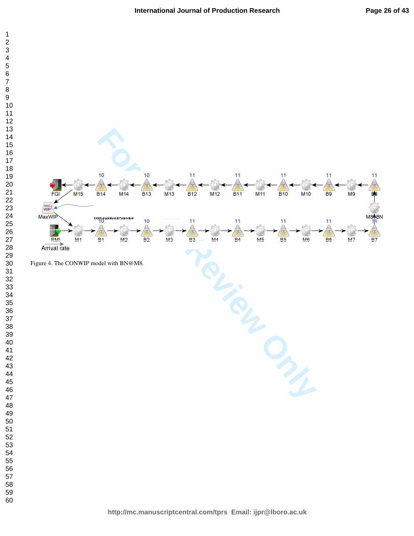
3.3 The CONWIP model

The CONWIP mechanism was first proposed by Spearman et al. (1990) as “a pull alternative to Kanban”. The

first machine in a line under CONWIP control is only authorized to begin production if the total number of

parts (i.e. WIP) in the line is less than a predetermined WIP level, or WIP cap. Hence, a CONWIP line can be

regarded as having a “long Kanban pull” that connects the end of the line to its beginning to maintain an

almost constant level of WIP in the system. Based on this “long pull” concept, the object for modeling

CONWIP in FACTS Analyzer is called “MaxWIP” because the WIP level is maintained at a maximum

degree by a long pull mechanism, as shown in Figure 6. In the example model considered here, by connecting

M15, the last machine, to the first machine, M1, a part leaving from M15 to the FGI will trigger the entry of a

new part to M1.

Figure 4. The CONWIP model with BN@M8.

In the CONWIP model, as well as the buffer capacities (subject to the same buffer constraint as the push

model), another important decision variable that must be optimized is the level of CONWIP. In other words, a

solution vector for the SMO of the CONWIP model can be represented as (B1, B2, …, BN, Ccap), where Ccap

represents the WIP cap in a CONWIP line. The determination of the optimal CONWIP level is the most

important parameter which influences the system performance, and a topic widely studied in the literature.

Page 9 of 43



123456789101112131415161718192021222324252627282930313233343536373839404142434445464748495051525354555657585960

For Peer Review O

nly


Nevertheless, as the comprehensive review of Framinan et al. (2003) indicates, the number of CONWIP

“cards” to be employed should involve a compromise between the desired throughput rate (or service level)

and other objectives, e.g. the WIP level. In general, many previous simulation studies have reported that

CONWIP outperforms Kanban by having a higher system throughput for a given level of total WIP; for

example, see (So 1990). However, the drawback that CONWIP does not take into account the impact a

bottleneck workstation may have on the performance of a production line was not considered adequately

(Graves et al. 1995). This topic can, however, be found in the literature that compares the application of

CONWIP to unbalanced lines with distinct bottlenecks controlled by the DBR mechanism.

3.4 The DBR model

The DBR mechanism operates in the manner that a constant level of WIP is maintained between the

bottleneck and the entrance of the line, instead of between the end of the line and the beginning of the line, as

in a CONWIP system. In other words, the first machine is authorized to start production if a part leaves the

bottleneck workstation. This mechanism is referred to as “drum-buffer-rope” because the bottleneck, as the

constraint that restricts the performance of the whole line, using the terms of the Theory of Constraint

(Blackstone and Cox 2002), should be the workstation that controls the pace (as the drum) of the other

workstations. The signaling mechanism that is connected from the bottleneck station to the front of the line,

pulling new jobs to the constrained workstation is called the “rope”. In this way, the operation of this “rope” is

identical to the long CONWIP pull that keeps the WIP cap between the constraint and the first workstation.

Applying this to our 15-workstation case study, in order to simulate a DBR model, if M8 is the bottleneck

station, then a MaxWIP object is used to act as the “drum” in the DBR controlled model; when a part leaves

Machine M8, a new part can be released to the line. In FACTS Analyzer, a DBR model can be made by

“wiring” the MaxWIP loop to the bottleneck machine (see Figure 5).

Figure 5. The DBR model with BN@M8.

The decision variables of the DBR models are the same as the CONWIP models, that is, solution vectors are

in the form of (B1, B2, …, BN, Ccap). Unlike the decision variable Ccap in the CONWIP model, Ccap here

represents the WIP level maintained between the bottleneck and M1. Besides the fact that the total buffer

Page 10 of 43



123456789101112131415161718192021222324252627282930313233343536373839404142434445464748495051525354555657585960

For Peer Review O

nly


capacity should be equal to 150, an additional constraint is added to the optimization to relate the buffer

capacity between the bottleneck and the front of the line because there is no point in having a maximum level

of WIP larger than the total sum of the buffer capacity and the number of machines before the immediate

downstream buffer of the bottleneck workstation:

3.5 The simulation and optimization settings

All the results generated in this paper are based on the approach of dynamic replication analysis that computes

the standard error of the output performance measures during the optimization processes. Simply put, instead

of using a fixed n, the optimization algorithm used in FACTS Analyzer will request more replications to be

run only if the computed error is found to be higher than the tolerable level. The relative precision approach is

employed to calculate the ratio of standard error of the data and the mean of the data from n replications,

based on the following formula:

1,12

1,12

relative precision

mean of the output performance measure from the replications

standard deviation of from the replications

Student-t distribution with

n

r

r

n

tn

x

where

x x n

x n

t

α

α

σ

µ

µ

σ

− −

− −

=

=

=

=

= degree of freedom 1 and probablity 1-2

nα

−

For the optimization results to be based on statistically robust output data, the standard error of the data should

be relatively small in comparison to the sample mean. Hence, 0.01 was chosen to be the tolerable value of µr

for both of the most important performance measures considered in this paper, namely average TP and

average CT. In order to be statistically correct, this implies all µr calculated from the simulation runs must be

lower than 0.009 (see Law and Kelton 2000 for the mathematical proof).

A variant of the NSGA-II algorithm (Deb et al. 2002), called MA-NSGA-II has been used to generate all the

{ }

-1

max

4,8,12 ,

m

iC b m

m

≤ +

=

∑i=1

where position of the bottleneck.

Page 11 of 43



123456789101112131415161718192021222324252627282930313233343536373839404142434445464748495051525354555657585960

For Peer Review O

nly


results presented in this paper. There are three major techniques that render the outstanding performance of

NSGA-II (Ding et al. 2008): (1) a “fast” non-dominated sorting approach that reduces the O(mN3) complexity

of MOGA to O(mN2) (Babbar et al. 2003); (2) a λ + µ elitism selection procedure and (3) the use of crowding

distance, as a measure for comparison and selection after the non-dominated sorting, to preserve the diversity

of the solutions in the population. In contrast to the original NSGA-II, MA-NSGA-II uses Artificial Neural

Networks (ANN) as the meta-modeling techniques for the rapid evaluation of candidate offspring solutions

for the purpose of filtering out those likely to be inferior. Additionally, MA-NSGA-II uses the Confidence-

based Significant Dominance (CSD) technique, first introduced in (Ng et al. 2008), to cope with the

simulation output data uncertainty.

The parameter settings used in the optimizations are shown in Table 1. Due to the stochastic searching of

evolutionary algorithms, it is important to repeat the optimization runs. Five optimization replications were

run for each of the models in this case study, and each optimization was replicated with some slight variation

in the mutation rate and crossover probability.

Table 1. Setting of the optimization parameters

MA-NSGA-II was run using an enlarged sampling space (µ+λ) selection strategy with the population sizes of

parents and offspring each equal to 100 (i.e. µ=λ=100) in all the optimization runs. In every generation, the µ

parents and the λ offspring competed for survival on the basis of CSD-based non-dominating sorting and

crowded distance tournament selection. Furthermore, in every generation, 500 candidate solutions were

generated. Rather than running expensive simulations for all of these candidate solutions, evaluations were

made using the ANN meta-model, which is a back-propagation feedforward net with one hidden layer. A fast

non-dominating sorting with CSD was employed to sort the candidates. The best λ candidates were then

selected to be the offspring solutions on the basis of the estimated values in the multi-objective functions.

Simulation runs were then performed on these λ candidates for accurate evaluations.

4. Results and Analysis

The CT-TP plot of the Pareto fronts for the Push model with various bottleneck (BN) positions is shown in

Figure 6. Every single curve in this CT-TP plot was obtained by collecting the best Pareto-optimal solutions

Page 12 of 43



123456789101112131415161718192021222324252627282930313233343536373839404142434445464748495051525354555657585960

For Peer Review O

nly


in the 5 optimization runs for that particular PCM and bottleneck location combination. This is called the best

attainment surface in EMO literature (Deb 2001). The graph clearly indicates that the location of the

bottleneck does have an effect on the line. For the Push model, the graph shows that if the slowest workstation

is closer to the front of the line then the same TP can be achieved with shorter CT. This effect is clear in the

lower and middle CT-TP regions, but not in the high CT-TP region where BN@M8 apparently seems to

outperform BN@M4. In order to verify these differences, we will introduce some methods to test the

statistical significance of the differences for the curves as well as between individual solutions in the CT-TP

plots.

A plot of TP against WIP is provided in Figure 7. Despite WIP not being one of the multiple objectives in the

optimization and the effect on the TP-WIP plot not being as pronounced as in the CT-TP plot, it is interesting

to observe that the TP-WIP plot resembles the pattern of the CT-TP graph. An important observation

concerning the characteristics of the Pareto-optimal solutions is apparent with the plot of CT against WIP, as

shown in Figure 8. Here it can be seen that a perfectly straight line is formed in the WIP-CT plot with all the

PF solutions. This linear relation between WIP and CT for the Pareto-optimal solutions not only exists for a

particular line design but for all the models tested in this study. This observation can be easily explained with

the help of Little’s Law, TP=WIP/CT.

Figure 6. CT-TP plot of the basic Push model with various bottleneck positions.

Figure 7. WIP-TP plot of Push control with various bottleneck positions.

Figure 8. WIP-CT plot of the Pareto-optimal solutions for the basic Push model with BN@M4.

Figure 9. Optimal CT-TP plot of the BN@M4 model with varying PCMs.



The effects of PCM on the line performance are further analyzed by visually comparing the optimal CT-TP

plots provided in Figures 9 to 11. The comparison indicates several important points that may affect the

selection of PCM for this particular 15-workstation production line under study:

• In general, irrespective of the location of the slowest workstation, DBR outperforms the three other

Page 13 of 43



123456789101112131415161718192021222324252627282930313233343536373839404142434445464748495051525354555657585960

For Peer Review O

nly


PCMs, particularly in the middle and high CT-TP region. This implies that DBR performs best in

terms of optimizing the trade-off between TP and CT, especially when the aim of the decision maker

is to achieve high TP. Together with the plots on varying bottleneck positions, it can be concluded that

using DBR with the slowest station closer to the upstream of a serial flow line is the best option in this

case study.

• It is clear that Push is an inferior option, especially if the decision maker focuses on the lower CT-TP

region. In Figures 10 and 11, the lower CT-TP region indicates that the poor performance of Push is

more pronounced when the bottleneck is closer to the end of the line; the Push control seems to be

more sensitive to the location of the bottleneck when compared to the three other PCMs. The

configuration of BN@M12 with Push control is the worst option in this comparison test.

• Kanban appears to be a good option if the aim of the decision maker is to have very low CT, but not if

high TP is desired. This observation is made because Kanban generally outperforms in the lower CT-

TP area (comparable to the performance of DBR), but produces poorly (with the same CT level) in the

middle and high CT-TP regions. It is interesting to note that there appears to be a distinct intersection

between the Push curve and the Kanban curve in the graph for BN@M12, as indicated in Figure 11.

• The effect of CONWIP is nearing DBR in the case of BN@M12. This is understandable because as

the bottleneck position approaches the end of the line, the location of the “Drum” to which the

“CONWIP signal” is sent will also be closer to the end of the line, and hence produces a similar effect

as in the CONWIP configuration. Otherwise, it can be seen that CONWIP is not apparently better or

even worse than Kanban in the lower CT-TP region.

While the optimization results indicate that PCM and the position of the bottleneck do affect the performance

of the line, and various PCMs have different effects in different regions of the optimal CT-TP plots,

conclusions about the PCM comparisons cannot be drawn simply by comparing the Pareto-optimal fronts

visually. There are two important questions which suggest that further analyses of the optimization results are

necessary for the PCM comparison.

• Can the Pareto fronts be compared using some quantitative metrics?

• How can the differences in the CT-TP curves be statistically verified?

These questions are answered with the introduction of the two methods in the following sub-sections.

Page 14 of 43



123456789101112131415161718192021222324252627282930313233343536373839404142434445464748495051525354555657585960

For Peer Review O

nly


4.1. Comparison using hypervolume and area under curve

Quantitative assessment of PF solutions in comparing the performance of different EMO algorithms is not an

easy task and there are many limitations in the performance indices proposed in EMO literature (Zitzler et al.

2002). A common metric used in EMO research for comparing a set of Pareto fronts generated by different

algorithms is the hypervolume, denoted as the S metric (Zitzler and Thiele 1998). Unlike many other

performance metrics, the S metric does not require the PFtrue to be known for its computation. For a bi-

objective optimization problem, the S metric is equivalent to the summation of all the rectangular areas

covered by the Pareto-optimal points, bounded by some reference point in the objective space.

Mathematically, the hypervolume can generally be described as below (Coello et al. 2007):

{ } i i knowni

S area vec PF= ∈U

Where veci is a non-dominated vector in the Pareto Front found in the optimization (PFknown) and areai is the

area between vector veci and the reference point (see Figure 12). The S metric is especially useful for

comparing both the convergence and the diversity of the PF generated for real-world complex optimization

problems in which the PFtrue is unknown. Furthermore, it offers many advantages such as multi-

dimensionality, i.e., able to cope with “many” objectives (>3) solution sets; compatibility with the

outperformance relations; capability for the differentiation between different degrees of complete

outperformance of two sets under comparison as well as scaling independency (Knowles and Corne 2001).

Figure 12. Calculating hypervolume for PCM comparison.

A novelty introduced in this study is that instead of using the S metric to compare the performance of different

EMO algorithms, it can be used to quantitatively compare the performance achieved when different PCMs are

applied to the same production line. This can be illustrated by the attainment surfaces in Figure 12, which

show the hypervolume produced by applying PCM A and PCM B on the CT-TP plot. An attainment surface is

the generated envelope for a set of non-dominating solutions, which is identical to the surface used to

calculate S (Deb 2001). By observing the attainment surfaces generated for the flow line using the PCM A and

PCM B under comparison, it can be seen that the comparison can be quantitatively made by comparing the

hypevolume that the PF has spread. In other words, the larger the S metric value, the higher the TP/CT ratio,

indicating that higher TP can be achieved with the same CT. With the example in Figure 12, the fact that

PCM A outperforms PCM B (see also Figure 1) can now be quantitatively verified by showing SA > SB. In

Page 15 of 43



123456789101112131415161718192021222324252627282930313233343536373839404142434445464748495051525354555657585960

For Peer Review O

nly


contrast to the technique that calculates the Trade-off Curves Areas (denoted as ∆ ) by assuming straight line

segments between the points along the trade-off curves (Enns 2007)(Enns and Roger 2008), hypervolume can

be readily applied to deal with problems that have more than two objectives. At the same time, without

knowing the existence of possible points between two consecutive solutions lying next to each other on the

Pareto front, it can be argued that assuming a straight line would increase the estimation error (Knowles

2008). It can obviously be seen that both the S and ∆ values for a Pareto front will also be dependent on the

position of the reference point selected by the decision maker, based on his/her region of interest in the

objective space.

The statistical accuracy of the S and ∆ metric required for the comparison is ensured by using the best

attainment surfaces obtained from the replicated optimization runs. At the same time, before the computation

of S and ∆ , normalizations have been done on the CT and TP values. This implies the maximum normalized

S or ∆ that can be obtained is of the value 1. For the 5 optimization runs (replications) carried out for each

PCM and BN combination, the normalized S and ∆ is therefore denoted as normS and

norm∆ . In contrast to the

original S calculation that uses only one reference point, another user-defined reference point is needed as the

base point for the normalizations (Reference point 2 in Figure 12). For a bi-objective min-min problem, (0,0)

can be selected as the base point by default, but this is not suitable for the CT-TP plot which is a min-max

problem. At the same time, the option of the reference points depends on the region of interest of the decision

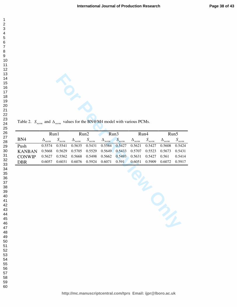
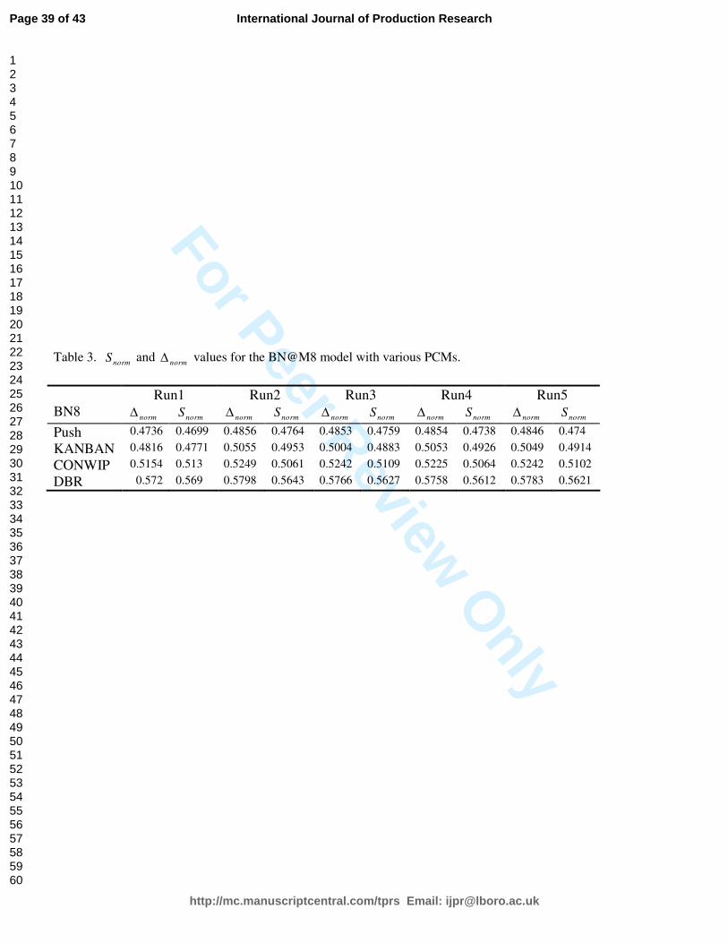
maker in the comparison. The normS and

norm∆ values of all the 60 optimization runs are shown in Tables 2 to

4 below. All of them were taken using the reference points (11000, 10.5) and (5000, 12.5) in the CT-TP space.

Table 2. normS and

norm∆ values for the BN@M4 model with various PCMs.

Table 3. normS and


Table 4. normS and


An analysis of the variance (ANOVA) test of the significance level α=0.05 was done to detect the significance

of the difference in the average of the normalized S and ∆ values, or normS and norm∆ respectively, obtained

from the replicated optimization runs. With all the F-statistic values >50 and p-value≈0, a significant

difference in performance can be deduced in the effect of the CT-TP plot when the four different PCMs are

applied. A post-ANOVA analysis, called the Duncan’s multiple range test, which is well-known for its

Page 16 of 43



123456789101112131415161718192021222324252627282930313233343536373839404142434445464748495051525354555657585960

For Peer Review O

nly


sensitivity to small differences between population sample means (see Mathews 2005, p.164), was applied to

determine which pairs of normS values are significantly different. The results obtained from the multiple range

test are summarized in Tables 5 to 7, where the value R is the calculated range of the values in a comparison

set and Rp is the Duncan’s least significant range value, determined by using the following equation:

, ,

, ,

where

standard error of the ANOVA

no. of replications

critical value for the test

p df

p

p df

s rR

n

s

n

r

ε

ε

ε α

ε

α

=

=

=

=

r is a value that depends on the significance level α = 0.05, the number of items in the comparison set,

p={4,3,2}, and the error degree of freedom dfε =16 for the ANOVA.

Table 5. Duncan’s multiple range test on normS and norm∆ for BN@M4


Table 7. Duncan’s multiple range test on normS and norm∆ or BN@M12

The results in Tables 6 to 8 can be interpreted as follows: if R > Rp, then the extreme values in the comparison

set are significantly different from each other. In many of the cases, it can be concluded from these statistical

tests that there are significant differences between the normS (and norm∆ ) spread by the solutions in PFknown. It

has confirmed that the observed differences resulting from the application of different PCMs are significant

after considering the replicated optimization runs. In general, DBR gives a significantly larger TP/CT ratio,

and is thus more desirable than the other three PCMs. CONWIP and Kanban are significantly better than

Push, but the difference between the CONWIP and Kanban cannot be statistically confirmed.

Page 17 of 43



123456789101112131415161718192021222324252627282930313233343536373839404142434445464748495051525354555657585960

For Peer Review O

nly


4.2 Comparison using CSD-based post-optimal analysis

Although the stochastic nature of the evolutionary algorithms can be handled by multiple optimization runs

when using S or ∆ , neither of these two methods has considered the uncertainty of individual optimal

solutions due to the randomness of simulation outputs in the objective space. In this paper, an innovative

comparison method, based on post-optimal analysis using CSD (Ng et al. 2008), is proposed. This method is

based on performing pairwise comparisons for all the solutions from the different models and PCM

combinations by applying the CSD sorting to all of the Pareto-optimal solutions from different Pareto sets. In

this case, the difference in the performance of different PCMs on the CT-TP plot can be statistically verified

and visualised. This method, called CSD-based post-optimal analysis, is particularly useful to statistically

verify the differences in the CT-TP curves which are close to each other or even apparently overlapping in the

objective space. In the results analysis done for the graph of BN@M12 in Figure 11, it indictaes that the

effect of CONWIP is very close to DBR in the BN@M12 model. At the same time, there appears to be a

crossover point between the Push curve and the Kanban curve in the graph of Figure 11. Two CSD-based

post-optimal analyses were therefore carried out for the BN@M12 model: (1) to collect all the solutions from

the four Pareto sets and (2) only the solutions from the Push and Kanban models. The aim of the first analysis

was to verify the outstanding behavior of DBR, the result of which is plotted in Figure 13. Despite the fact

that there seems to be some overlapping between the CONWIP and DBR curves, the CSD-based comparison

proves that most of the DBR solutions are significantly better than any other PCMs, including CONWIP,

except in the low CT-TP region where Kanban solutions dominate. This also verifies the superiority of

Kanban in the lower CT-TP area, as observed in the earlier results analysis for Figure 11.

The crossover between the Push and Kanban curves is verified by the CSD-based comparison, illustrated in

Figure 14, showing which solutions in the Push and Kanban Pareto sets significantly dominate. It clearly

shows that Kanban excels in the CT-TP trade-off below the (8000, 11.45) point, but Push solutions dominate

thereafter. This result is particularly interesting to demonstrate the importance of comparing PCMs in a

Pareto-optimal context, because a PCM may be preferable in a certain region but not others, depending on the

level of the primary interest of the decision maker (who may prefer low CT than high TP in some situations).

It is therefore necessary to generate the Pareto fronts and then study the performance behavior of the PCM in

different areas of the objective space.

Figure 13. CSD-based analysis for all the optimal solutions of the BN@M12 model with different varying PCMs.

Figure 14. CSD-based analysis for all the optimal solutions of the BN@M12 Push and Kanban models.

Page 18 of 43



123456789101112131415161718192021222324252627282930313233343536373839404142434445464748495051525354555657585960

For Peer Review O

nly


6. Conclusions and Outlook

The paper has illustrated the concept of comparing PCMs in their optimal parameter setting in a Pareto-based

multi-objective context using a case study of a buffer allocation problem in an unbalanced flow line. While

the numerical results of the case study cannot be generalized, there are two important conclusions that can be

drawn from the SMO results: (1) in terms of optimizing the trade-off between production rate and cycle time,

PCM plays a significant role; for example, this case study has shown that DBR generally outperforms Push

and classical pull mechanisms, such as Kanban and CONWIP; (2) comparing PCMs in a multi-objective

context is important, because a PCM may be preferable in certain regions, in the performance space, but not

others, depending on the primary interest of the decision maker. For example, in contrast to the common

understanding that Pull-based PCM is always better than Push, it has been shown in this case study that Push

outperforms Kanban if the target of the decision maker is on high production rate.

This paper has also introduced the use of hypervolume, a common performance metric for comparing the

performance of EMO algorithms, for the quantitative comparison of PCMs in the performance space. The

CSD-based post-optimality analysis is useful to complement such a quantitative test to statistically verify and

visualize the differences in the performance space, in particular when the solutions in the Pareto sets are close

to each other or even seemingly overlapping. The CSD-based analysis was particularly useful in this case

study in verifying the crossover point between Kanban and Push in the performance space.

The case study presented in this paper addresses a bi-objective dual OBA problem. It should be noted that the

same method can readily be applied to include other objectives, such as to minimize the total number of

buffers, for the purpose of minimizing the investment of buffers for a given desirable production rate and

cycle time. Applying the SMO methodology proposed in this paper, a comprehensive empirical study is now

underway using FACTS Analyzer. Other than the combination of PCMs and the locations of the bottleneck

tested in the current paper, we are particularly interested in examining how other factors would affect the

performance of an unbalanced production system. These factors include: (1) the number of

workstation/process steps (N) of the flow line; (2) the “strength” of the bottleneck; (3) the variability of the

line’s processing time following distribution other than log-normal and (4) including a downtime modeled

explicitly in both exponential and non-exponential distribution.

Page 19 of 43



123456789101112131415161718192021222324252627282930313233343536373839404142434445464748495051525354555657585960

For Peer Review O

nly


References

Andijani, A.A. and Anwarul, M., Manufacturing blocking discipline: A multi-criterion approach for buffer allocations. International Journal of Production Economics, 1997, 51, 155-163.

April, J., Better, M., Glover, F. and Kelly, J., New advances and applications for marrying simulation and optimization. In Proceedings of Winter Simulation Conference, 2004, Ingalls, R.G., Rossetti, M.D., Smith, J.S. & Peters, B.A. (eds.), Washington, D.C., USA, 80-86.

Altiparmak, F., Dengiz, B. and Bulgak, A.A., Optimization of buffer sizes in assembly systems using intelligent techniques. In Proceedings of Winter Simulation Conference, Yücesan, E., Chen, C.-H., Snowdon, J.L. & Charnes, J.M. (eds.), 2002, Piscataway, New Jersey, USA: IEEE, 1157-1162.

Altiparmak, F., Dengiz, B. and Bulgak, A.A., Buffer allocation and performance modeling in asynchronous assembly system operations: an artificial neural network metamodeling approach. Applied Soft Computing, 2007, 7(3), 946-956.

Babbar, M., Lakshmikantha, A. and Goldberg, D.E., A modified NSGA-II to solve noisy multiobjective problems. In Proceedings of Genetic and Evolutionary Computation Conference (GECCO). 12-16 July 2003, Chicago, Illinois, USA, 21-27.

Blackstone, J.H., Jr. and Cox, J.F.C., III, Designing unbalanced lines - understanding protective capacity and protective inventory. Production Planning & Control, 2002, 13(4), 416-423.

Bonvik, A.M., Couch, C.E. and Gershwin, S.B., A comparison of production-line control mechanisms. International Journal of Production Research, 1997, 35(3), 789-804.

Bulgak, A.A., Diwan, P.D. and Inozu, B., Buffer size optimization in asynchronous assembly systems using genetic algorithms. Computers and Industrial Engineering, 1995, 28(2), 309-322.

Buzacott, J.A. and Shanthikumar, J.G. Stochastic models of manufacturing systems Englewood Cliffs, 1993 (Prentice Hall: New Jersey).

Can, B., Beham, A. and Heavey, C., A comparative study of genetic algorithm components in simulation-based optimization. In Proceedings of Winter Simulation Conference, Mason, S.J., Hill, R.R., Mönch, L., Rose, O., Jefferson, T. & Fowler, J.W. (eds.), 2008, Miami, Florida, USA, 1829-1837.

Chan, F.T.S. and Ng, E.Y.H., Comparative evaluations of buffer allocation strategies in a serial line. International Journal of Advanced Manufacturing Technology, 2002, 19, 789-800.

Coello Coello, C.A., Lamont, G.B. and Veldhuizen, D.A.V., 2007. Evolutionary algorithms for solving multi-objective problems, 2nd edition, 2007, Springer.

Conway, R., Maxwell, W., Mcclain, J.O. and Thomas, L.J., The role of work-in-process inventory in serial production lines. Operations Research, 1988, 36, 229-241.

Deb, K., Multi-objective optimization using evolutionary algorithms, 3rd ed., 2001 (Wiley: Wiltshire, UK).

Deb, K., Pratap, A., Agarwal, S. and Meyarivan, T., A fast and elitist multi-objective genetic algorithm: NSGA-II. IEEE Transaction on Evolutionary Computation, 2002, 6(2), 181-197.

Ding, H., Benyoucef, L. and Xie, X., Stochastic multi-objective production-distribution network design using simulation-based optimization. International Journal of Production Research, 2008, 47(2), 479-505.

Dudley, N.A., Work time distributions. International Journal of Production Research, 1963, 2(2), 137-144.

Page 20 of 43



123456789101112131415161718192021222324252627282930313233343536373839404142434445464748495051525354555657585960

For Peer Review O

nly


Enns, S.T., "Pull" Replenishment performance as a function of demand rates and setup times under optimal settings. In Proceedings of Winter Simulation Conference, Henderson, S.G., Biller, B., Hsieh, M.-H., Shortle, J., Tew, J.D. & Barton, R.R. (eds.), 2007, Miami, Florida, USA, 1624-1632.

Enns, S.T. & Rogers, P., Clarifying CONWIP versus push system behavior using simulation. 2008 Winter Simulation Conference, Mason, S.J., Hill, R.R., Mönch, L., Rose, O., Jefferson, T. & Fowler, J.W. (eds.), 2008, Miami, Florida, USA, 1867-1872.

Framinan, J.M., González, P.L. and Ruiz-Usano, R., The CONWIP production control system: review and research issues. Production Planning & Control, 2003, 14(3), 255-265.

Gaury, E.G.A., Pierreval, H. and Kleijnen, J.P.C., An evolutionary approach to select a pull system among Kanban, CONWIP and hybrid. Journal of Intelligent Manufacturing, 2000, 11, 157-167.

Geraghty, J. and Heavey, C., A comparison of hybrid push/pull and CONWIP/pull production inventory control policies. International Journal of Production Economics, 2004, 91, 75-90.

Gershwin, S.B., An efficient decomposition method for the approximate evaluation of tandem queues with finite storage space and blocking. Operation Research, 1987, 35(2), 291-305.

Graves, R.J., Konopka, J.M. and Milne, R.J., Literature review of material flow control mechanisms. Production Planning & Control, 1995, 6(5), 395-403.

Hillier, F.S. and So, K.C., The effect of the coefficient of variation of operation times on the allocation of storage space in production line systems. IIE Transactions, 1991, 23, 198-206.

Hodgson, T.J. and Wang, D., Optimal hybrid push/pull control strategies for a parallel multi-stage system: Part I. International Journal of Production Research, 1991, 29(6), 1279–1287.

Hopp, W.J. and Spearman, M.L., Factory physics: foundations of manufacturing management, 2nd ed., 2000 (Irwin McGraw-Hill Higher Education: Burr Ridge, IL).

Kim, S., Davis, K.R. and Cox, J.F., An investigation of output flow control, bottleneck flow control and dynamic flow control mechanisms in various simple lines scenarios. Production Planning & Control, 2003, 14(1), 15-32.

Koh, S.-G. and Bulfin, R.L., Comparison of DBR with CONWIP in an unbalanced production line with three stations. International Journal of Production Research, 2004, 42(2), 391-404.

Knowles, J. and Corne, D., On metrics for comparing non-dominated sets. Congress on Evolutionary Computation (CEC 2002), Piscataway, NJ: IEEE Press, 711-716.

Knowles, J., A summary-attainment-surface plotting method for visualizing the performance of stochastic multiobjective optimizers. In Proceedings of the 5th International Conference on Intelligent Systems Design and Applications (ISDA), 8-10 September 2005, Wroclaw, Poland, IEEE Computer Society, 552-557.

Lacksonen, T., Empirical comparison of search algorithms for discrete event simulation. Computers and Industrial Engineerring, 2001, 40(1-2), 133-148.

Laguna, M. and Martí, R., The OptQuest callable library. In Optimization software class libraries. Boston: Kluwer Academic Publishers, Voß, S. & Woodruff, D. eds., 2002, 193-218.

Laguna, M. and Martí, R., Scatter search: Methodology and implementations in C, 2003 (Kluwer Academic Publishers: Boston).

Law, A.M. and Kelton, W.D., Simulation Modeling and Analysis, 3rd ed., 2000 (McGraw-Hill Higher Education).

Little, J.D.C., Are there ‘Laws’ of Manufacturing, Manufacturing Systems? In Foundations of World-Class Practice, J. A. Heim and W. D. Compton (eds.), National Academy Press, Washington, D.C., 1992, 180–188.

Page 21 of 43



123456789101112131415161718192021222324252627282930313233343536373839404142434445464748495051525354555657585960

For Peer Review O

nly


Lutz, C.M., Davis, K.R. and Sun, M., Determining buffer location and size in production line using Tabu search. European Journal of Operation Research, 1998, 106, 301-316.

MacDonald, C. & Gunn, E., A simulation based system for analysis and design of production control systems. In Proceedings of Winter Simulation Conference, Mason, S.J., Hill, R.R., Mönch, L., Rose, O., Jefferson, T. & Fowler, J.W. (eds.), 2008, Miami, Florida, USA, 1882-1890.

Mathews, P., Design of experiments with Minitab, 2005 (ASQ Quality Press). Ng, A., Urenda, M., Svensson, J., Skoogh, A. and Johansson, B. (2007) FACTS Analyser: An

innovative tool for factory conceptual design using simulation, In Proceedings of Swedish Production Symposium 2007 (SPS’07), Gothenburg, 28-30 August 2007.

Ng, A., Syberfeldt, A, Grimm, H. and Svensson, J. (2008) Multi-Objective Simulation Optimization and Significant Dominance for Comparing Production Control Mechanisms, In 18th International Conference on Flexible Automation and Intelligent Manufacturing (FAIM’08), Skövde, Sweden, pp. 1210-1219.

So, K.C., 1997. Optimal buffer allocation strategy for minimizing work-in-process inventory in unpaced production lines. IIE Transactions, 29, 81-88.

Spearman, M.L., Woodruff, D.L. & Hopp, W.J., 1990. CONWIP: A pull alternative to Kanban. International Journal of Production Research, 28 (5), 879-894.

Spinellis, D.D. and Papadopoulos, C.T., 2000a. A simulated annealing approach for buffer allocation in reliable production lines. Annals of Operations Research, 93, 373-384.

Spinellis, D.D. and Papadopoulos, C.T., 2000b. Stochastic algorithms for buffer allocation in reliable production lines. Mathematical Problems in Engineering, 5, 441-458.

Takahashi, K., Morikawa, K. & Chen, Y.-C., 2007. Comparing Kanban control with the theory of constraints using Markov chains. International Journal of Production Research, 45 (16), 3599-3617.

Zitzler, E. and L. Thiele (1998). Multiobjective optimization using evolutionary algorithms —a comparative case study. In A. E. et al. (Ed.), Parallel Problem Solving from Nature, Berlin, Germany, pp. 292–301. Springer.

Zitzler, E., Laumanns, M., Thiele, L., Fonseca, C.M. and Fonseca, V.G.D., 2002. Why quality assessment of multiobjective optimizers is difficult. Proceedings of the Genetic and Evolutionary Computation Conference. Morgan Kaufmann Publishers Inc., 666-674.

Page 22 of 43



123456789101112131415161718192021222324252627282930313233343536373839404142434445464748495051525354555657585960

For Peer Review O

nly

Figure 1. Comparing two PCMs with their Pareto-optimal settings in a CT-TP plot.

Page 23 of 43



123456789101112131415161718192021222324252627282930313233343536373839404142434445464748495051525354555657585960

For Peer Review O

nly

Figure 2. The push model with BN@M8.

Page 24 of 43



123456789101112131415161718192021222324252627282930313233343536373839404142434445464748495051525354555657585960

For Peer Review O

nly

Figure 3. The Kanban model with BN@M8.

Page 25 of 43



123456789101112131415161718192021222324252627282930313233343536373839404142434445464748495051525354555657585960

For Peer Review O

nly

Figure 4. The CONWIP model with BN@M8.

Page 26 of 43



123456789101112131415161718192021222324252627282930313233343536373839404142434445464748495051525354555657585960

For Peer Review O

nly

Figure 5. The DBR model with BN@M8.

Page 27 of 43



123456789101112131415161718192021222324252627282930313233343536373839404142434445464748495051525354555657585960

For Peer Review O

nly

Figure 6. CT-TP plot of the basic Push model with various bottleneck positions.

Page 28 of 43



123456789101112131415161718192021222324252627282930313233343536373839404142434445464748495051525354555657585960

For Peer Review O

nly

Figure 7. WIP-TP plot of Push control with various bottleneck positions.

Page 29 of 43



123456789101112131415161718192021222324252627282930313233343536373839404142434445464748495051525354555657585960

For Peer Review O

nly

Figure 8. WIP-CT plot of the Pareto-optimal solutions for the basic Push model with BN@M4.

Page 30 of 43



123456789101112131415161718192021222324252627282930313233343536373839404142434445464748495051525354555657585960

For Peer Review O

nly


Page 31 of 43



123456789101112131415161718192021222324252627282930313233343536373839404142434445464748495051525354555657585960

For Peer Review O

nly


Page 32 of 43



123456789101112131415161718192021222324252627282930313233343536373839404142434445464748495051525354555657585960

For Peer Review O

nly


Page 33 of 43



123456789101112131415161718192021222324252627282930313233343536373839404142434445464748495051525354555657585960

For Peer Review O

nly

Figure 12. Calculating hypervolume for PCM comparison.

Page 34 of 43



123456789101112131415161718192021222324252627282930313233343536373839404142434445464748495051525354555657585960

For Peer Review O

nly

Figure 13. CSD-based analysis for all the optimal solutions of the BN@M12 model with different varying PCMs.

Page 35 of 43



123456789101112131415161718192021222324252627282930313233343536373839404142434445464748495051525354555657585960

For Peer Review O

nly

Figure 14. CSD-based analysis for all the optimal solutions of the BN@M12 Push and Kanban models.

Page 36 of 43



123456789101112131415161718192021222324252627282930313233343536373839404142434445464748495051525354555657585960

For Peer Review O

nly

Table 1. Setting of the optimization parameters

Total number of simulations 5000

Population size (µ) 100

Child population size (λ) 100

Number of candidates 500

Mutation rate 0.05-0.15 (with step in 0.05)

Crossover probability 0.5-0.7 (with step of 0.1)

Crossover operator Uniform

Page 37 of 43



123456789101112131415161718192021222324252627282930313233343536373839404142434445464748495051525354555657585960

For Peer Review O

nly

Table 2. norm

S and norm

∆ values for the BN@M4 model with various PCMs.

Run1 Run2 Run3 Run4 Run5

BN4 norm

∆ norm

S norm

∆ norm

S norm

∆ norm

S norm

∆ norm

S norm

∆ norm

S

Push 0.5574 0.5541 0.5635 0.5431 0.5584 0.5427 0.5621 0.5427 0.5608 0.5424

KANBAN 0.5668 0.5629 0.5705 0.5529 0.5649 0.5433 0.5707 0.5523 0.5673 0.5431

CONWIP 0.5627 0.5562 0.5668 0.5498 0.5662 0.5493 0.5631 0.5427 0.561 0.5414

DBR 0.6057 0.6031 0.6076 0.5924 0.6071 0.591 0.6051 0.5909 0.6072 0.5917

Page 38 of 43



123456789101112131415161718192021222324252627282930313233343536373839404142434445464748495051525354555657585960

For Peer Review O

nly

Table 3. norm

S and norm



BN8 norm

∆ norm

S norm

∆ norm

S norm

∆ norm

S norm

∆ norm

S norm

∆ norm

S

Push 0.4736 0.4699 0.4856 0.4764 0.4853 0.4759 0.4854 0.4738 0.4846 0.474

KANBAN 0.4816 0.4771 0.5055 0.4953 0.5004 0.4883 0.5053 0.4926 0.5049 0.4914

CONWIP 0.5154 0.513 0.5249 0.5061 0.5242 0.5109 0.5225 0.5064 0.5242 0.5102

DBR 0.572 0.569 0.5798 0.5643 0.5766 0.5627 0.5758 0.5612 0.5783 0.5621

Page 39 of 43



123456789101112131415161718192021222324252627282930313233343536373839404142434445464748495051525354555657585960

For Peer Review O

nly

Table 4. norm

S and norm



BN12 norm

∆ norm

S norm

∆ norm

S norm

∆ norm

S norm

∆ norm

S norm

∆ norm

S

Push 0.4077 0.4032 0.3948 0.329 0.3923 0.326 0.402 0.389 0.398 0.3197

KANBAN 0.4077 0.4018 0.3882 0.3731 0.3829 0.3655 0.3818 0.3657 0.3609 0.3353

CONWIP 0.5038 0.5009 0.4639 0.4491 0.4638 0.4487 0.4625 0.4444 0.4622 0.4461

DBR 0.5229 0.52 0.4829 0.4595 0.4835 0.4628 0.4842 0.4673 0.4828 0.4667

Page 40 of 43



123456789101112131415161718192021222324252627282930313233343536373839404142434445464748495051525354555657585960

For Peer Review O

nly


normS norm∆

Comparison set R R > Rp R R > Rp

DBR, CONWIP, Kanban,

Push

0.0488 Yes 0.0461 Yes

DBR, CONWIP, Kanban 0.0459 Yes 0.0426 Yes

DBR, CONWIP 0.0429 Yes 0.0426 Yes

CONWIP, Kanban 0.0030 No 0.0030 Yes

Kanban, Push 0.0076 Yes 0.0059 No

Page 41 of 43



123456789101112131415161718192021222324252627282930313233343536373839404142434445464748495051525354555657585960

For Peer Review O

nly


normS norm∆



Push

0.0899 Yes 0.0936 Yes


DBR, CONWIP 0.0545 Yes 0.543 Yes

CONWIP, Kanban 0.0204 Yes 0.0227 Yes

Kanban, Push 0.0149 Yes 0.0166 Yes

Page 42 of 43



123456789101112131415161718192021222324252627282930313233343536373839404142434445464748495051525354555657585960

For Peer Review O

nly

Table 7. Duncan’s multiple range test on normS and norm∆ or BN@M12

normS norm∆



Push

0.1219 Yes 0.107 Yes


DBR, CONWIP 0.0174 No 0.02 No

CONWIP, Kanban 0.0896 Yes 0.0869 Yes

Kanban, Push 0.0149 No 0.0146 No

Page 43 of 43



123456789101112131415161718192021222324252627282930313233343536373839404142434445464748495051525354555657585960

a comparative study of production control mechanisms using

Documents