a compact articial bee colony optimization for topology...

Journal of Information Hiding and Multimedia Signal Processing c©2015 ISSN 2073-4212

Ubiquitous International Volume 6, Number 2, March 2015

A Compact Articial Bee Colony Optimization forTopology Control Scheme in Wireless Sensor

Networks

Thi-Kien Dao, Tien-Szu Pan∗ and Trong-The Nguyen

Department of Electronic EngineeringNational Kaohsiung University of Applied Sciences

415 Chien-Kung Road, Kaohsiung, 807, Taiwan∗Corresponding author

[email protected]; [email protected]; [email protected]

Shu-Chuan Chu

School of Computer Science, Engineering and MathematicsFlinders University

[email protected]

Received July, 2014; revised November, 2014

Abstract. In this paper, a compact Articial Bee Colony optimization method (cABC)for applying to the topology optimization of wireless sensor networks (WSNs) is presented.The purpose of compact algorithms is to address to the computational requirements in thelimited resources of hardware devices such as memory size or low price. A probabilisticrepresentation random of the collection behavior of social bee colony is inspired to employfor this proposed algorithm. The real population is replaced with the probability vectorupdated based on single competition. These lead to a modest memory usage when the en-tire algorithm is applied. Four selected test functions are used to evaluate the accuracy,computational time and memory saving of the proposed method. The experimental re-sults show that the proposed cABC method is not only as accurate as the existing originalArticial Bee Colony optimization but also requires less calculative time than the origi-nal method and uses a modest memory with only six agents needed for storing space.In addition, compared with the genetic algorithm (GA) method and the particle swarmoptimization (PSO) method, the proposed cABC method can provide the highest robuststructure and lowest contention topology schemes.Keywords: Bee colony algorithm, Compact artificial bee colony algorithm, Optimiza-tions, Swarm intelligence, Topology control, Wireless sensor networks.

1. Introduction. Computational intelligence algorithms have been used to solve opti-mization problems in engineering, financial, and management fields. For example, geneticalgorithms (GA) have been used successfully in engineering, financial, and security [1-3]. Particle swarm optimization (PSO) and enhanced PSO techniques [4-6] have beenemployed to forecast the exchange rates, segment images, optimize multiple interferencecancellations [7-9], construct the portfolios of stock, and segment color images based onhuman perception [3, 10, 11]. Ant colony optimization (ACO) techniques have been uti-lized to solve the routing problem of networks and secure watermarking [12, 13]. Artificialbee colony (ABC) and Interactive Artificial Bee Colony have been used to solve the nu-merical problems and support the passive continuous authentication systems [14, 15]. Cat

297

298 T. K. Dao, T. S. Pan, S. C. Chu, and T. T. Nguyen

swarm optimization (CSO) techniques have been used to solve the numerical problems,the aircraft schedule, and the lot-streaming flow shop scheduling problem [16-18] and dis-cover proper positions for information hiding [19], respectively. In addition, bat algorithm(BA) is used for engineering design [20] and classifications[21]. Some applications requirethe solution of a complex optimization problem in limited hardware conditions causedby the cost and space constraints of computational devices. For example, wireless sensornetworks (WSNs) are the networks of small, battery-powered, and memory-constraintdevices (i.e., sensor nodes). Due to memory and power constraints, they need to be wellarranged to build a fully functional network to have the capability of wireless communi-cation in a restricted area [22]. For telecommunications [23] and energy production [13],a fast solution of the optimization problem is required. In addition, space shuttle control[24] and underwater communication [25] require high fault-tolerance and the avoidance ofdevice rebooting. However, computational devices do not have enough memory to store apopulation composed of numerous candidate solutions of those computational intelligencealgorithms for the aforementioned applications.

Compact algorithms are a promising answer to hardware limitations because they use anefficient compromise to present some advantages of population-based algorithms withoutstoring an actual population of solutions. Compact algorithms simulate the behavior ofpopulation-based algorithms by employing their probabilistic representation instead of apopulation of solutions. Consequently, compact algorithms require less memory to storethe number of parameters compared to their corresponding population-based structures.

The rst implementation of compact algorithms is the compact Genetic Algorithm (cGA)[26]. The cGA simulates the behavior of a standard binary encoded Genetic Algorithm(GA). The performance of cGA is almost as good as that of GA and requires less memory.The compact Differential Evolution (cDE) algorithm has been introduced in [11]. Thesuccess implementation of cDE is based on the combination of two factors. First, a cDEscheme benets from the introduction of a certain degree of randomization due to theprobabilistic model. Second, the one-to-one spawning survivor selection typical of cDE(the offspring replaces the parent) can be naturally encoded into a compact logic.

The compact Particle Swarm Optimization (cPSO) has been dened in [27]. The im-plementation of cPSO algorithm benets from the same natural encoding of the selectionscheme employed by cDE and another ingredient of compact optimization, i.e., a spe-cial treatment for the best solution ever detected and reinterpreted as an evolutionaryalgorithms in order to propose a compact encoding of PSO.

In this paper, the behavior and the characteristic of the bees are reviewed to improvethe Artificial Bee Colony algorithms [16, 28] and to present the compact Artificial BeeColony Algorithm (cABC) based on the framework of the original Artificial Bee Colony(oABC). According to the experimental results, our proposed cABC presents the sameresult in finding solutions as the original Artificial Bee Colony algorithm [29].

Moreover, WSNs, an emerging and promising technology, have been widely used in avariety of long-term and critical applications [30]. However, sensor nodes are limited inthe computation capability and storage capacity of a computing unit, the communicationrange and radio quality of a communication unit, the sensing coverage and accuracy ofa sensing unit, and the available energy of a power unit [31]. Topology control is one ofthe most fundamental problems in WSNs. It is an effective factor to ensure the quality ofconnectivity and coverage because it determines how to maintain network connectivity andtransmit the power of each node while consuming as minimum power as possible. The newproposed cABC method would be applied to find out the solution for the topology controlscheme in WSNs. The topology control scheme could be transformed into the problem ofmulti-objective degree-constrained minimum spanning tree. The multi-objective strategy

A cABC Optimization for Topology Control Scheme in WSNs 299

with a fitness function based on a niche and phenotype sharing function is also appliedin cABC to obtain an approximation of the true Pareto front.

The rest of this paper is organized as follows: a brief review of ABC is given in Section2; the statement of topology control in WSNs is reviewed in Section 3; the analysis anddesign for the cABC is presented in Section 4; the experimental results and the comparisonbetween oABC and cABC are discussed in Section 5; the application of cABC for topologycontrol is presented in Section 6; finally, the conclusion is made in Section 7.

2. The Artificial Bee Colony algorithm. The Artificial Bee Colony algorithm wasproposed by Karaboga in 2005 [23], and the performance of ABC was analyzed in 2008[24] by inspecting the behaviors of real bees on finding nectar and sharing the informationof food sources to the bees in the nest. There are three kinds of bees defined in ABCas being the artificial agents known as the employed bee, the onlooker, and the scout.Every kind of these bees plays a different and important role in the optimization process.For example, the employed bee stays on a food source, which represents a spot in thesolution space, and provides the coordinate for the onlookers in the hive for reference.The onlooker bee receives the locations of the food sources and selects one of the foodsources to gather the nectar. The scout bee moves in the solution space to discover newfood sources.

The process of ABC optimization is listed as follows:Step 1. Initialization: Spray ne percentage of the populations into the solution space

randomly, and then calculate their fitness values, namely nectar amounts, where ne rep-resents the ratio of employed bees to the total population. Once these populations arepositioned into the solution space, they are called the employed bees. The fitness valueof the employed bees is evaluated to take account in their amount of nectar.

Pi =F (θi)∑Sk=1 F (θk)

(1)

Step 2. Move the Onlookers: Calculate the probability of selecting a food source byequation (1), where θi denotes the position of the ith employed bee, F (θi) denotes thefitness function, S represents the number of employed bees, and Pi is the probability ofselecting the ith employed bee. The roulette wheel selection method is used to select afood source to move for onlooker bees and then determine their nectar amounts. Theonlookers are moved by equation (2), where xi denotes the position of the ith onlookerbee, t denotes the iteration number, is the randomly chosen employed bee, j representsthe dimension of the solution, and Φ(.) produces a series of random variable in the rangefrom -1 to 1.

xij(t+ 1) = θij (t) + Φ(θij (t)− θkj (t)) (2)

Step 3. Update the Best Food Source Found So Far: Memorize the best fitness valueand the position, which are found by the bees.

Step 4. Move the Scouts: If the fitness values of the employed bees are not improvedby a continuous predetermined number of iterations, namely Limit, those food sourcesare abandoned, and these employed bees become the scouts. The scouts are moved byequation (3), where r is a random number and r ∈ [0, 1].

θij = θjmin + r × (θjmax − θjmin) (3)

Step 5. Termination Checking: Check if the amount of the iterations satisfies thetermination condition. If the termination condition is satisfied, terminate the programand output the results, otherwise go back to Step2.

The main steps of the algorithm are as below:


1. Initialize Population2. repeat3. Place the employed bees on their food sources4. Place the onlooker bees on the food sources depending on their nectar amounts5. Send the scouts to the search area to discover new food sources6. Memorize the best food source found so far7. until requirements are met

3. Topology control scheme for wireless sensor networks. A wireless sensor net-work is modeled as a directed, connected graph G = (V,E), where V is a nite set ofvertices (sensor nodes), V = {v1, v2, ..vn} and E is the set of edges (network links), rep-resenting connection of these vertices, E = {e1,2, e1,3, ..ei,j, ..en−1,n} . Let n = |V | be thenumber of network nodes and l = |E| be the number of network links. The linke = (vi, )from node vi ∈ V to node vj ∈ V implies the existence of a link e′ = (, vi) from node vjto node vi. A link can be defined as follows:

ei,j =

{1, if vi, vj have edge

0, otherwise(i = 1, 2, .., n− 1; j = i+ 1, 2, .., n) (4)

If the edge of ei,j exists, this edge has l associated positive real numbers. There areattributes in WSNs that weights could be defined on [28] [29]. Representing the weightcould be denoted wki,j =

{w1ij, w

2ij, ..w

lij

}, where k = 1, 2, , l. There l positive real value

functions are associated with each linke(e ∈ E) such as: cos C(e) : E → R+, cover-age B(e) : E → R+, delay D(e) : E → R+, data fusion F (e) : E → R+, loss rateL(e) : E → R+, power consumption P (e) : E → R+ , etc. The link cost function, C(e),may be either monetary cost or any measures of resource utilization that must be opti-mized. The link coverage, B(e), is the reachable sensing radius of the sensors. The linkdelay, D(e), is considered to be the sum of switching modes, queuing, transmission, andpropagation delays. The link data fusion,F (e), is the aggregation and integration datafunctions. The link loss rate, L(e), is the packet loss rate on the receiving end on link e.The link power consumption, P (e), is the energy for transiting, receiving and processingsignals. These attributes B(e), D(e), F (e), L(e), P (e) dene the criteria that must be con-strained (bounded) because the sensor nodes are limited resources. Let PT (s, d) be pathin the tree T from the source node s to a destination node d ∈ M . Let m = |M | be thenumber of multi-criteria destination nodes, where M is the destination group and s ∪Mis the multi-criteria group. Let α be the coverage constraint, β be the delay constraint, δbe the data aggregation constraint, ζ be the loss rate constraint, and η be the dissipatedenergy constraint. The multi-constrained least-cost multi-criteria problem is defined asfollows:

MinimizeC(T (s,M)) subjects to:

Bxi,yi(X) ≤ α ∀ d ∈M ;D(PT (s, d)) ≤ β ∀ d ∈M ;F (PT (s, d)) ≤ δ ∀ d ∈M ;

L(PT (s, d)) ≤ ζ ∀ d ∈M ;P (PT (s, d)) ≤ η ∀ d ∈M(5)

A spanning tree of graph G can be expressed by the vector x.Letx = (x1,2, x1,3, . . . , xi,j, . . . xn−1,n)

xi,j =

{1, if ei,j = 1 and selected

0, otherwise(i = 1, 2, . . . , n− 1; j = i+ 1, 2, . . . , n) (6)

A multi-criteria tree T (s,M) is a subgraph of G spanning the source node s ∈ V and theset of destination nodes M ⊆ V −{s}. Let X be the set of all such vectors corresponding


to spanning trees in graph G. The multi-criteria degree constrained minimum spanningtree problem can be formulated as follows:

min f1 (x) =∑w1i,jxi,j

min f2 (x) =∑w2i,jxi,j

. . .min fm (x) =

∑wli,jxi,j

(i = 1, 2, .., n− 1; j = i+ 1, . . . n)1 ≤

∑wli,jxi,j ≤ d

(x ∈ X; i = 1, 2, .., n; j = 1, 2, . . . n)

(7)

where fi(x) is the ith objective to be minimized for the problem and d denotes thedegree constraint. Wireless sensor network may suffer from poor network utilization,high end-to-end delays, and short network lifetime if its topology control scheme is notproper in a right place.

4. The proposed Compact Artificial Bee Colony (cABC) method. As mentionedabove, compact algorithms process an actual population of solution as a virtual popula-tion. This virtual population is encoded within a data structure, namely PerturbationVector (PV) as probabilistic model of a population of solutions. The distribution of in-dividuals in the hypothetical swarms must be described by a probability density function(PDF) [30] defined on the normalized interval from -1 to +1. The distribution of each beein the swarms could be assumed as Gaussian PDF with mean µ and standard deviationδ [20]. A minimization problem is considered in an m-dimensional hyper-rectangle innormalization of two truncated Gaussian curves (m is the number of parameters). With-out loss of generality, the parameters are assumed to be normalized so that each searchinterval ranges from -1 to +1. Therefore, PV is a vector of m2 matrix specifying the twoparameters of the PDF of each design variable. PV is defined as:

PV t =[µt, δt

](8)

where µ and δ are mean and standard deviation values of a Gaussian (PDF) truncatedwithin the interval range from -1 to +1, respectively. The amplitude of the PDF isnormalized in order to keep its area equal to 1. The apex t is time step. The initializationof the virtual population is generated for each design variable i, µ1

i = 0 and δ1 = k, wherek is set as a large positive constant (e.g., k = 10). The PDF height normalization isobtained sufficiently in the uniform distribution with a wide shape. The generating fora candidate solution xi is produced from PV (µi, δ). The value of mean µ and standarddeviation δ in PV are associated to the equation of a truncated Gaussian PDF as follows:

PDF (trucNormal (x)) =e− (x−µi)

2

2δ2i

√2π

δi(erf(ui+1√2δi

)− erf

(ui−1√2δi

))

(9)

The PDF in equation (9) is then used to compute the corresponding Cumulative Dis-tribution Function (CDF). The CDF is constructed by means of Chebyshev polynomialsby following the procedure described in [31]. The codomain of CDF ranges from 0 to 1.CDF is defined as a real-valued random variable X with a given probability distributionat a value less than or equal to xi, as shown in equation (10). CDFs are also used tospecify the distribution of multivariate random variables.


CDF =

1∫0

e− (x−µi)

2

2δ2i

√2π

δi(erf(ui+1√2δi

)− erf

(ui−1√2δi

))dx (10)

The sampling of the design variable xi from PV is performed by generating a randomnumber rand [0, 1] from a uniform distribution and then computing the inverse functionof CDF in rand [0, 1]. The newly calculated value is xi by the sampling mechanism asequation (11):

xi = inverse(CDF ) (11)

When the comparison between two design variables for individuals of the swarm (orbetter two individuals sampled from PV) is performed the winner solution biases the PV.The vector that scores a better tness value is regarded as the winner; the individual losingthe (tness based) comparison is defined as the loser. Regarding the mean values l, theupdate rule for each of its elements is µti, δ

ti => µt+1

i , δt+1i

µt+1i = µti +

1

Np

(winneri − loseri) (12)

where Np is virtual population size. Regarding δ values, the update rule of each elementis given by:

δt+1i =

√(δti)

2 + (µti)2 −

(µt+1i

)2+

1

Np

(winner2i − loser2i ) (13)

[winner, loser] = complete(xbest, x

t+1)

(14)

The construction of equations (13) and (14) are persistent and non-persistent structureswith tested results given in [32]. Similar to the binary cGA case, it was impossible toassess whether one or another elitist strategy was preferable. In elitist compact schemes,each moment of the optimum performance is retained in a separate memory slot. If anew candidate solution is computed, the tness-based comparison between it and the eliteis carried out. If the elite is a winner solution, it biases the PV as shown in formulas (13)and (14).

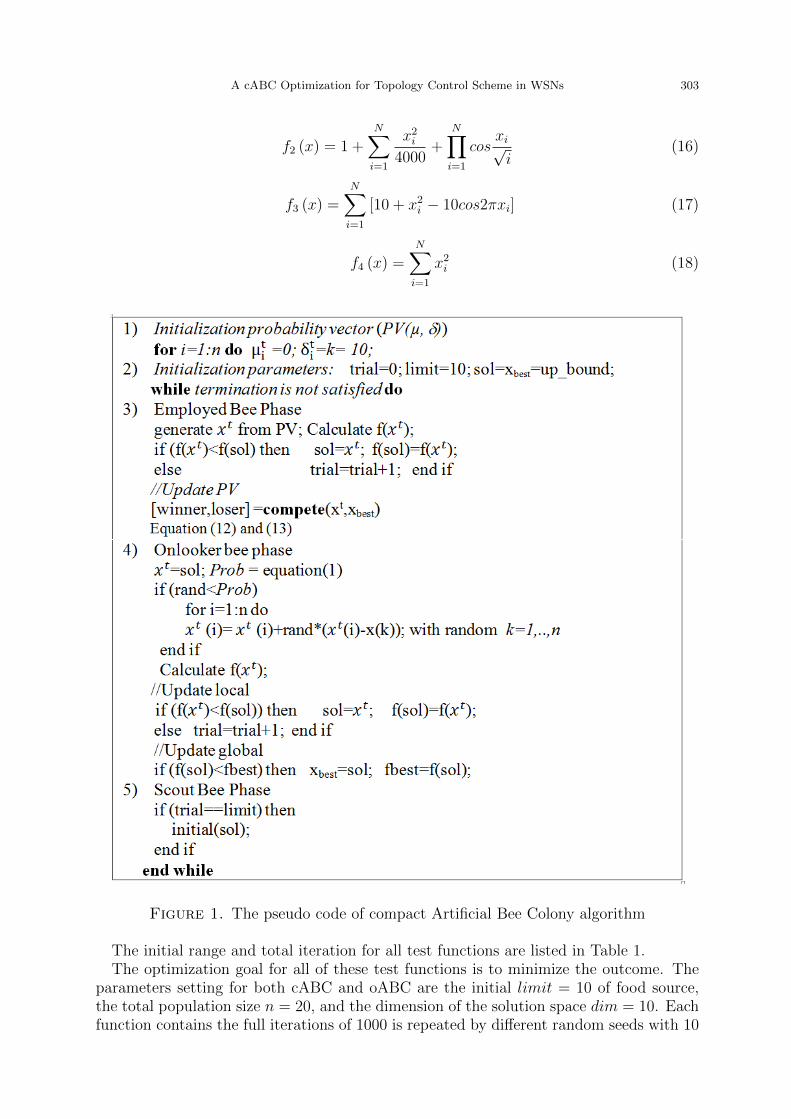
Figure 1 shows the pseudo code of algorithm working principles of cABC. The tnessvalue of the position xt is calculated and compared with xbest to determine a winnerand a loser. Equations (13) and (14) are then applied to update the probability vectorPV. If rand is smaller than Prob (probability equation (1) is calculated from employmentbee phrase), xt will be calculated by equation (2). Update local and update global areimplemented in Onlooker bee phrase. If f(sol) < fbest, the value of function is memorized,and the value of the global best is then updated.

5. Experimental results. This section presents the simulation results in running bench-mark function tests and compares the cABC with the oABC, both in terms of solutionquality and the number of memory variables evaluations taken. Four test standard func-tions are chosen for the experiments to evaluate the accuracy and computational speedof the proposed cABC. All experiments are averaged over different random seeds with10 runs. The test standard functions used include Rosenbrock, Griewank, Rastrigin, andSphere, which are listed in equations (15) to (18).

f1 (x) =n−1∑i=1

(100(xi−1 − x2i

)2+ (1− xi)2 (15)


f2 (x) = 1 +N∑i=1

x2i4000

+N∏i=1

cosxi√i

(16)

f3 (x) =N∑i=1

[10 + x2i − 10cos2πxi] (17)

f4 (x) =N∑i=1

x2i (18)

Figure 1. The pseudo code of compact Artificial Bee Colony algorithm

The initial range and total iteration for all test functions are listed in Table 1.The optimization goal for all of these test functions is to minimize the outcome. The

parameters setting for both cABC and oABC are the initial limit = 10 of food source,the total population size n = 20, and the dimension of the solution space dim = 10. Eachfunction contains the full iterations of 1000 is repeated by different random seeds with 10


Table 1. The initial range and the total iteration of test standard functions

FunctionsInitial range

[xmax, xmin]Total iterations

Rosenbrock f1 (x) [ -30,30] 1000Griewangk f2 (x) [ -100,100] 1000Rastrigin f3 (x) [-5.12,5.12 ] 1000Spherical f4 (x) [ -100,100 ] 1000

runs. The final result is obtained by taking the average of the outcomes from all runs.The results are compared with the original ABC.

5.1. Comparing optimizing performance algorithms. Table 2 shows the compari-son of the quality of performance and time running for numerical problem optimizationbetween cABC and oABC. It is obvious that the average cases of the testing functionsin compact Artificial Bee algorithm converge faster than the original cases. The mean offour test functions on the evaluation of minimum function for 10 runs is 6.78E+07 withaverage time consuming 1.174 s for oABC and 3.29E+07 with average time consuming0.341 s for cABC.

Table 2. The comparison between oABC and cABC in terms of perfor-mance quality and speed

FunctionsPerformance as mean of

evaluationTime running

evaluation (seconds)oABC cABC oABC cABC

f1 (x) 1.79E+08 1.75E+08 0.7503 0.2118f2 (x) 0.2987 0.3615 1.0895 0.2457f3 (x) 137.8214 139.2473 0.6979 0.2075f4 (x) 2.2582 2.6112 0.6241 0.1891

Average value 1.79E+08 1.76E+08 3.1618 0.8541

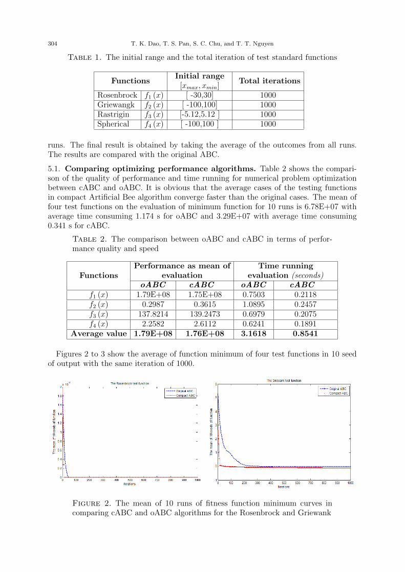
Figures 2 to 3 show the average of function minimum of four test functions in 10 seedof output with the same iteration of 1000.

Figure 2. The mean of 10 runs of fitness function minimum curves incomparing cABC and oABC algorithms for the Rosenbrock and Griewank


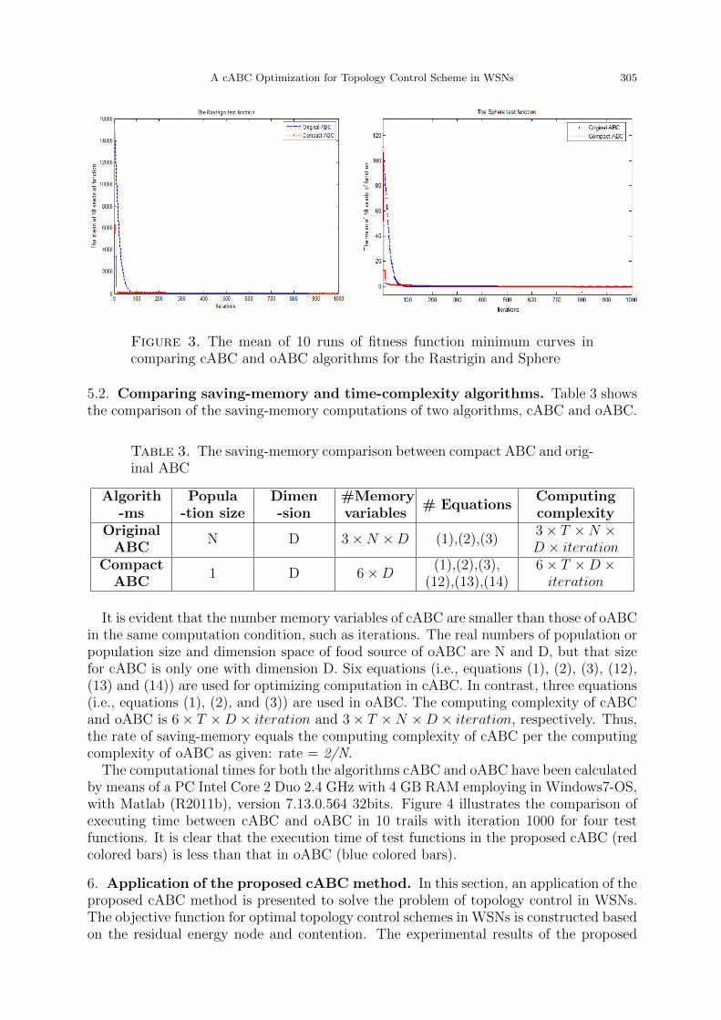
Figure 3. The mean of 10 runs of fitness function minimum curves incomparing cABC and oABC algorithms for the Rastrigin and Sphere

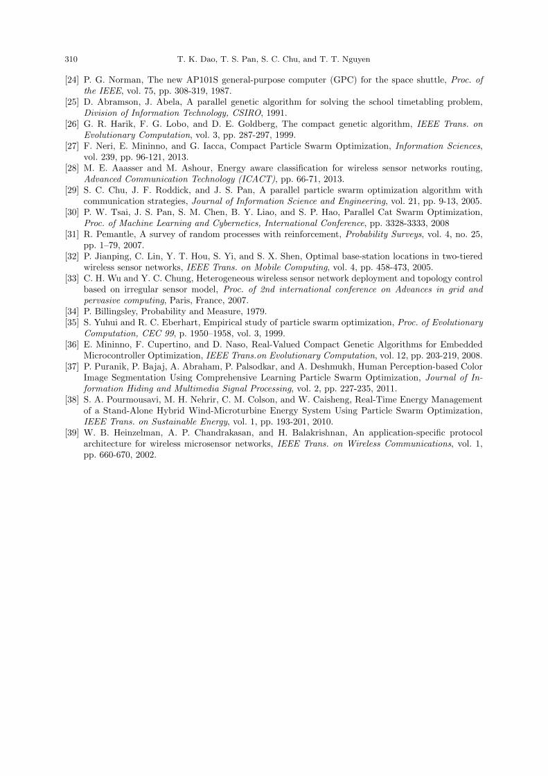
5.2. Comparing saving-memory and time-complexity algorithms. Table 3 showsthe comparison of the saving-memory computations of two algorithms, cABC and oABC.

Table 3. The saving-memory comparison between compact ABC and orig-inal ABC

Algorith-ms

Popula-tion size

Dimen-sion

#Memoryvariables

# EquationsComputingcomplexity

OriginalABC

N D 3×N ×D (1),(2),(3)3× T ×N ×D × iteration

CompactABC

1 D 6×D (1),(2),(3),(12),(13),(14)

6× T ×D ×iteration

It is evident that the number memory variables of cABC are smaller than those of oABCin the same computation condition, such as iterations. The real numbers of population orpopulation size and dimension space of food source of oABC are N and D, but that sizefor cABC is only one with dimension D. Six equations (i.e., equations (1), (2), (3), (12),(13) and (14)) are used for optimizing computation in cABC. In contrast, three equations(i.e., equations (1), (2), and (3)) are used in oABC. The computing complexity of cABCand oABC is 6× T ×D × iteration and 3× T ×N ×D × iteration, respectively. Thus,the rate of saving-memory equals the computing complexity of cABC per the computingcomplexity of oABC as given: rate = 2/N.

The computational times for both the algorithms cABC and oABC have been calculatedby means of a PC Intel Core 2 Duo 2.4 GHz with 4 GB RAM employing in Windows7-OS,with Matlab (R2011b), version 7.13.0.564 32bits. Figure 4 illustrates the comparison ofexecuting time between cABC and oABC in 10 trails with iteration 1000 for four testfunctions. It is clear that the execution time of test functions in the proposed cABC (redcolored bars) is less than that in oABC (blue colored bars).

6. Application of the proposed cABC method. In this section, an application of theproposed cABC method is presented to solve the problem of topology control in WSNs.The objective function for optimal topology control schemes in WSNs is constructed basedon the residual energy node and contention. The experimental results of the proposed


Figure 4. Comparison of two algorithms in term of time running for test functions

method is compared with the PSO-Optimized Minimum Spanning Tree-Based TopologyControl Scheme method in [33] and the Genetic Algorithm (GA) for Multi-criteria Mini-mum Spanning Tree Problem in [34].

6.1. Network Model Description. As mentioned in section 4, a network model couldbe described as following: a wireless sensor network with n nodes is randomly distributedin desired areas. Each node can communicate with others by using transmission ranger. That is, node i can receive the signal of node j if node i is in the transmissionrange r of node j. The topology of the network is abstracted by nodes with their ownmaximum transmission range as a directed graph, denoted by G =< V,E > in whichV = {V1, V2, .., Vn} is the set of node numbers, and E = {E1, E2, .., En} is the set ofconnectable communication between any of two nodes.

Let D(i, j) be the Euclidean distance of nodes i and j in the network and CNi bethe set of connectable neighbors which communicate with node i by using its maximumwireless transmission range rmax. For each node i that belongs to V , let Gi =< Vi, Ei >be an induced sub-graph of G in which Vi = CNi, Ei is the subset of E. Consequently,Gi is the connectable node graph of node i.

Let C(i, r) be the coverage of an edge, that is, the disk centered at node i with its certainradius r. Node i could affect at least all nodes located in the area of radius r = D(i, j),centered at node i. The coverage of an edge between node i and node j is the measure ofthe number of nodes covered by the disk established by i and j [35].

Li,j = [{Vi ∈ V |D(Vi, i) ≤ R1}]∪ [Vj ∈ V |D(Vj, j) ≤ R2)] (19)

where R1 and R2 are the radius of C(i, r) and C(j, r), respectively. The strength of anedge between node i and node j is defined as:

Si,j =ei × ej√e2i + e2j

(20)

where ei and ej are the remaining energy of node i and j, respectively.Local minimum spanning tree of node i is implemented based on the set of connectable

neighbors Gi. It is assumed that E = {E1,2, E1,3, ..., Ei,j, ..., En−1,n} is the set of edgesconstructed by Gn =< Vn, En > . If the connection can be formed between nodes Viand Vj, then Ei,j = E,ji = 1. Otherwise, Ei,j = E,ji = 0, where ∀Vi, Vj ∈ Gn; i =1, 2, 3, ..., n; j = i+ 1, ..., n . The energy consumption between nodes Vi and Vj is definedasPi,j = kdβ, where k is the system constant, d is the communication distance, and the


value of β is often predefined constant as the path loss exponent with value setting from 2to 4. Each edge has a positive real number, Wi, defined as the weight of a communicationlink and calculated as the result of a topology with the aspects of low energy consumption,high stable structure, and low communication interference:

Wi,j = α1 ×Pi,jSi,j

+ α2 × Li,j (21)

where α1 and α2 are the predefined parameters and α1 + α2 = 1. A spanning tree ofgraphGn can be expressed by vectorX as shown in equation (6), which can be transformedinto the optimization problem for the minimal fitness function as shown in equation (7),which in turn can be formulated as the following equation:

Fitnessi =∑

Wi,j × xi,j (22)

In reality, because the network topology in WSNs may vary with time as a result of manyuncertain factors, the network topology is adjusted every ∆t time. At the same time,uni-directional edges can be removed or some extra edges can be added in order to geta final topology consisting of only bi-directional edges. The coordinates of vertices in Gand the weights of each edge are generated randomly. Each edge in the graph is supposedto have only two weights with real numbers

6.2. Experimental results and comparison. The environmental setting is as follows:the range of deployment of network is 100X100m, the number of objectives is 2, andthe number of vertices is 20. The setting parameters for both the proposed cABC-WSNstopology and oABC-WSNs topology are as follows: the initial limit of food source is 10,the total population size n is 20, and the dimension of the solution space dim is 10. Eachfunction contains 1000 full iterations for each of the 10 random seeds. The experimentalparameters for PSO-WNS topology are c1 = c2 = 2.0, inertia weight w is 0.9, populationsize is 20, and the maximum iteration times is 1000 in each run [36]. The parametersfor the GA-WSNs topology are set as follows: population size is 20, crossover probabilitypc is 0.2, mutation probability pm is 0.05, and maximum generation max gen is 1000 ineach run [1, 34]. The final result is obtained by taking the average of the outcomes from10 runs. The experimental results of cABC-WSNs are compared with the results of ABC(ABC-WSN topology), GA (GA-WSN topology), and PSO (PSO-WSN topology).

Table 4 shows that the average convergent time of the fitness functions in the cABCmethod (9.288 minutes) is 30% faster than that of the oABC method (12.086 minutes).While cABC-WSNs topology evidently outperforms oABC-WSNs topology in time con-sumption, the mean of fitness functions evaluation of minimum function for 10 runs ob-tained using the cABC method is almost as good as that obtained using the oABC method.In addition, it is much more accurate than the means obtained using the GA-WSNs topol-ogy and PSO-WSNs topology by 16% and 8%, respectively.

Figure 5 illustrates the comparison of the cABC-WSNs topology method with theoABC-, PSO-, and GA-WSNs topology methods.

It is obvious that the performance of fitness functions evaluation values for 10 runsusing the cABC-WSNs topology and oABC-WSNs topology are faster convergence thanthe performance using the GA-WSNs topology and PSO-WSNs topology.

7. Conclusion. In this paper, a novel optimization algorithm, namely compact ArtificialBee Colony algorithm (cABC), was presented. The implementation of compact optimiza-tion algorithms is significant for the development of small-sized and low-cost embeddeddevices. It fits the trend of ubiquitous computing today. In this new proposed algorithm,


Table 4. The comparison of the proposed cABC-WSN topology with theGA-WSNs topology, the PSO-WSNs topology, and the oABC-WSNs topol-ogy in terms of quality performance evaluation and speed

MethodsPopulation

sizeObjectives Vertices

Averagefunctionvalues

Consum-ption

times(m)The GA-WSNstopology (Han &Wang 2005, with

cm-MST)

20 2 20 8.6023 22.086

The PSO-WSNstopology (Wenzhonget al., 2013, with

cm-MST)

20 2 20 7.2091 11.086

The oABC-WSNstopology

20 2 20 5.9434 12.086

The cABC-WSNstopology

1 2 20 6.0921 9.288

Figure 5. The averages of minimum value of fitness function for 10 runsobtained using the cABC-, oABC-, PSO-, and GA-WSNs topology meth-ods.

the actual design solutions for search space for Artificial Bee Colony algorithm is replacedwith a virtual population, which is a probabilistic representation of the population. Thisfeature is essential for applications with a limited memory such as the embedded imple-mentation in small and inexpensive devices. The performance of cABC algorithm is asgood as the other compact algorithms in previous works in literature. The results of theproposed algorithm on a set of various test problems show that cABC is a valid alternativefor optimization problems with a limited memory. The proposed method is also appliedto solve the problem of topology control in WSNs. Compared with the GA method andthe PSO method, the proposed cABC method provides the most robust structure and


lowest contention topology schemes. The experimental results show the proposed cABCas an effective memory-saving algorithm.

REFERENCES

[1] L. Davis (ed), Handbook of genetic algorithms, vol. 115, New York: Van Nostrand Reinhold, 1991.[2] S. Wang, B. Yang, and X. Niu, A Secure Steganography Method based on Genetic Algorithm,

Journal of Information Hiding and Multimedia Signal Processing, vol. 1, pp. 28-35, 2010.[3] R. J. Kuo, C. H. Chen and Y. C. Wang, An intelligent stock trading decision support system through

integration of genetic algorithm based fuzzy neural network and artificial neural network, Fuzzy Setsand Systems, vol. 1, no. 118, pp. 21-45, 2001.

[4] R. Eberhart, J. Kennedy, Particle swarm optimization, vol. 4, pp. 1942-1948, 1995.[5] H. Wang, H. Sun, C. Li, S. Rahnamayan, and J. S. Pan, Diversity enhanced particle swarm opti-

mization with neighborhood search, Information Sciences, vol. 223, pp. 119-135, 2013.[6] C. Sun, J. Zeng, J. Pan, S. Xue, and Y. Jin, A new fitness estimation strategy for particle swarm

optimization, Information Sciences, vol. 221, pp. 355-370, 2013.[7] S. M. Chen and C. Y. Chien, Solving the traveling salesman problem based on the genetic simu-

lated annealing ant colony system with particle swarm optimization techniques, Expert Systems withApplications, vol. 38, pp. 14439-14450, 2011.

[8] C. H. Hsu, W. J. Shyr, and K. H. Kuo, Optimizing Multiple Interference Cancellations of LinearPhase Array Based on Particle Swarm Optimization, Journal of Information Hiding and MultimediaSignal Processing, vol. 1, pp. 292-300, October 2010.

[9] S. Yuhui and R. Eberhart, A modified particle swarm optimizer, Proc. of Evolutionary ComputationProceedings, IEEE World Congress, Computational Intelligence , pp. 69-73, 1998.

[10] J. F. Chang and S. W. Hsu, The Construction of Stock’s Portfolios by Using Particle Swarm Opti-mization, Innovative Computing Information and Control ICICIC ’07, Proc. of Second InternationalConference, pp. 390-390, 2007.

[11] E. Mininno, F. Neri, F. Cupertino, and D. Naso, Compact Differential Evolution, IEEE Trans. onEvolutionary Computation, vol. 15, pp. 32-54, 2011.

[12] P. C. Pinto, A. Nagele, M. Dejori, T. A. Runkler, and J. M. Sousa, Using a Local Discovery AntAlgorithm for Bayesian Network Structure Learning, IEEE Trans. on Evolutionary Computation,vol. 13, no. 4, pp. 767-779, 2009.

[13] J. Y. Chouinard, K. Loukhaoukha, and M. H. Taieb, Optimal Image Watermarking AlgorithmBased on LWT-SVD via Multi-objective Ant Colony Optimization, Journal of Information Hidingand Multimedia Signal Processing, vol. 2, no. 4, pp. 303-319, 2011.

[14] D. Karaboga, An idea based on honey bee swarm for numerical optimization, Technical Report-TR06,Erciyes University, Engineering Faculty, Computer Engineering Department, vol. 200, 2005.

[15] P. W. Tsai, M. K. Khan, J. S. Pan, and B. Y. Liao, Interactive Artificial Bee Colony SupportedPassive Continuous Authentication System, IEEE, Systems Journal, vol. 8, pp. 395-405, 2014.

[16] Y. T. Hou, S. Yi, H. D. Sherali, and S. F. Midkiff, On energy provisioning and relay node placementfor wireless sensor networks, IEEE Trans. on Wireless Communications, vol. 4, pp. 2579-2590, 2005.

[17] P. W. Tsai, J. S. Pan, S. M. Chen, and B. Y. Liao, Enhanced parallel cat swarm optimization basedon the Taguchi method, Expert Systems with Applications, vol. 39, pp. 6309-6319, 2012.

[18] S. C. Chu, P. W. Tsai, and J. S. Pan, Cat Swarm Optimization, PRICAI 2006, Trends in ArtificialIntelligence, Springer Berlin Heidelberg, vol. 4099, pp. 854-858, 2006.

[19] Z. H. Wang, C. C. Chang, and M. C. Li, Optimizing least-significant-bit substitution using cat swarmoptimization strategy, Inf. Sci., vol. 192, pp. 98-108, 2012.

[20] M. Younis, M. Youssef, and K. Arisha, Energy-aware routing in cluster-based sensor networks, Mod-eling, Analysis and Simulation of Computer and Telecommunications Systems, IEEE InternationalSymposium, pp. 129-136, 2002.

[21] G. Qingbo, F. Shuxing, and M. Yanhua, A Network Topology Clustering Algorithm for ServiceIdentification, Proc. of International Conference Computer Science and Service System (CSSS), pp.1583-1586, 2012.

[22] I. F. Akyildiz, S. Weilian, Y. Sankarasubramaniam, and E. Cayirci, A survey on sensor networks,IEEE, Communications Magazine, vol. 40, pp. 102-114, 2002.

[23] G. Cheung, W. T. Tan, and T. Yoshimura, Real-time video transport optimization using streamingagent over 3G wireless networks, IEEE Trans. on Multimedia, vol. 7, no.4, pp. 777-785, 2005.


[24] P. G. Norman, The new AP101S general-purpose computer (GPC) for the space shuttle, Proc. ofthe IEEE, vol. 75, pp. 308-319, 1987.

[25] D. Abramson, J. Abela, A parallel genetic algorithm for solving the school timetabling problem,Division of Information Technology, CSIRO, 1991.

[26] G. R. Harik, F. G. Lobo, and D. E. Goldberg, The compact genetic algorithm, IEEE Trans. onEvolutionary Computation, vol. 3, pp. 287-297, 1999.

[27] F. Neri, E. Mininno, and G. Iacca, Compact Particle Swarm Optimization, Information Sciences,vol. 239, pp. 96-121, 2013.

[28] M. E. Aaasser and M. Ashour, Energy aware classification for wireless sensor networks routing,Advanced Communication Technology (ICACT), pp. 66-71, 2013.

[29] S. C. Chu, J. F. Roddick, and J. S. Pan, A parallel particle swarm optimization algorithm withcommunication strategies, Journal of Information Science and Engineering, vol. 21, pp. 9-13, 2005.

[30] P. W. Tsai, J. S. Pan, S. M. Chen, B. Y. Liao, and S. P. Hao, Parallel Cat Swarm Optimization,Proc. of Machine Learning and Cybernetics, International Conference, pp. 3328-3333, 2008

[31] R. Pemantle, A survey of random processes with reinforcement, Probability Surveys, vol. 4, no. 25,pp. 1–79, 2007.

[32] P. Jianping, C. Lin, Y. T. Hou, S. Yi, and S. X. Shen, Optimal base-station locations in two-tieredwireless sensor networks, IEEE Trans. on Mobile Computing, vol. 4, pp. 458-473, 2005.

[33] C. H. Wu and Y. C. Chung, Heterogeneous wireless sensor network deployment and topology controlbased on irregular sensor model, Proc. of 2nd international conference on Advances in grid andpervasive computing, Paris, France, 2007.

[34] P. Billingsley, Probability and Measure, 1979.[35] S. Yuhui and R. C. Eberhart, Empirical study of particle swarm optimization, Proc. of Evolutionary

Computation, CEC 99, p. 1950–1958, vol. 3, 1999.[36] E. Mininno, F. Cupertino, and D. Naso, Real-Valued Compact Genetic Algorithms for Embedded

Microcontroller Optimization, IEEE Trans.on Evolutionary Computation, vol. 12, pp. 203-219, 2008.[37] P. Puranik, P. Bajaj, A. Abraham, P. Palsodkar, and A. Deshmukh, Human Perception-based Color

Image Segmentation Using Comprehensive Learning Particle Swarm Optimization, Journal of In-formation Hiding and Multimedia Signal Processing, vol. 2, pp. 227-235, 2011.

[38] S. A. Pourmousavi, M. H. Nehrir, C. M. Colson, and W. Caisheng, Real-Time Energy Managementof a Stand-Alone Hybrid Wind-Microturbine Energy System Using Particle Swarm Optimization,IEEE Trans. on Sustainable Energy, vol. 1, pp. 193-201, 2010.

[39] W. B. Heinzelman, A. P. Chandrakasan, and H. Balakrishnan, An application-specific protocolarchitecture for wireless microsensor networks, IEEE Trans. on Wireless Communications, vol. 1,pp. 660-670, 2002.

a compact articial bee colony optimization for topology...

Documents