a combined cfd-dsmc method for numerical simulation of nozzle plume flows

A COMBINED CFD-DSMC METHOD FOR

NUMERICAL SIMULATION OF NOZZLE PLUME

FLOWS

A Dissertation

Presented to the Faculty of the Graduate School

of Cornell University

in Partial Fulfillment of the Requirements for the Degree of

Doctor of Philosophy

by

Jyothish D George

January 2000

c© Jyothish D George 2000

ALL RIGHTS RESERVED

The objective of this dissertation was to develop a methodology for performing

simulations of a complete nozzle plume system. The combined approach involves

four steps. First, a continuum simulation of the nozzle plume system is performed.

An unstructured Navier-Stokes solver for performing these simulations was devel-

oped. The next step involves predicting the breakdown of Navier-Stokes equations

from the CFD simulations and dividing the domain into a CFD region and a

DSMC region. Various parameters that could be used for this were investigated

and a new parameter was proposed. The third step involves transferring infor-

mation from the CFD simulation to the DSMC simulation. Different methods of

transferring information were analyzed. The last step involves performing DSMC

simulations. DSMC simulations were performed and the results were analyzed to

understand more about the breakdown of the Navier-Stokes equations.

The method was applied to the study of two nozzle systems for which experi-

mental results were available. The first system involved was a hydrogen thruster.

A kinetics model for hydrogen consistent with a previously developed DSMC model

was implemented. It was successfully applied to investigate the low-density hydro-

gen plume flows. The comparison between the numerical results and experimental

measurements was found to be good in terms of overall flow features. For a more

detailed quantitative comparison higher resolution experimental measurements are

required. An important conclusion of this study is that these solutions exhibit a

high degree of grid dependence. This was found to be true of both the DSMC and

CFD computations. Thus care should be taken to ensure that the grid resolution is

fine enough to obtain accurate results. This emphasizes the importance of flexible

gridding techniques provided by the use of unstructured grids. For this system, it

is difficult to separate the results of the grid dependence from the physics of the

problem.

The next system analyzed was the expansion of carbon di-oxide into vacuum.

The computational results were found to be sensitive to the wall boundary condi-

tion. Experimental measurements of pitot pressure measurements along the cen-

terline were compared with calculations based on the CFD simulations. The com-

puted values were close enough to experimental measurements to suggest that the

physics of the flow was captured accurately. Detailed relaxation modeling of the

different energy modes of CO2 indicated that the vibrational mode was frozen in

the diverging portion of the nozzle and in the plume. The CFD simulations also

predicted regions of rotational non-equilibrium inside the plume. The central core

region of the flow was non-isentropic and had a ratio of specific heats, γ close

to 1.2. This invalidates the isentropic flow assumption and the value of γ of 1.4

used for calibrating some of the experimental measurements. The computations

re-confirmed earlier findings about the behavior of the flow near the nozzle lip.

Flow angle measurements were compared with the computed values and found to

agree in the central-core region of the flow. The CFD predictions of radial pro-

files of number density showed good agreement within regions of validity of the

continuum approach.

A breakdown parameter was used to split the domain by predicting the break-

down of the Navier-Stokes equations. DSMC simulations were performed of regions

where CFD methods are not accurate, were performed. The DSMC predictions of

radial number density profiles were then compared with the experimental mea-

surements and found to be in good agreement, even in regions where the CFD

results disagree with experiments. DSMC results were analyzed in detail in an

attempt to investigate the failure of the CFD approach. It was found that the re-

gions where CFD results are inaccurate corresponded with regions of translational

non-equilibrium. Since the Navier-Stokes equations are based on the assumption

of translational equilibrium, solutions to Navier-Stokes equations give inaccurate

results for such flow regimes.

Biographical Sketch

iii

This is dedicated to my mother and father, sisters and brothers, aunts and

uncles, cousins, grandparents, etc. Oh yes, and my 6th grade math teacher who

thought I would never get past 7th grade math.

iv

Acknowledgements

I would like to acknowledge the fantastic help and support of all of those who

helped and supported me. Without their tireless help and support I would have

not been able to do this fine work.

Finally, I gratefully acknowledge the efforts of Dr. James Drakes in being in-

strumental in the release of the AEDC report for public distribution. This research

has been supported by the Army Research Office Grant DAAG55-98-1-0500 and

by NASA Lewis Research Center Grant NAG3-1958.

v

Table of Contents

1 Motivation and Background 11.1 Introduction . . . . . . . . . . . . . . . . . . . . . . . . . . . . . . . 11.2 Objectives and Scope of this work . . . . . . . . . . . . . . . . . . . 3

2 Description of the combined approach 52.1 Introduction . . . . . . . . . . . . . . . . . . . . . . . . . . . . . . . 52.2 Description of methodology . . . . . . . . . . . . . . . . . . . . . . 62.3 CFD Simulations . . . . . . . . . . . . . . . . . . . . . . . . . . . . 62.4 Chapman-Enskog Parameter . . . . . . . . . . . . . . . . . . . . . . 72.5 DSMC Simulations . . . . . . . . . . . . . . . . . . . . . . . . . . . 72.6 Outline of thesis . . . . . . . . . . . . . . . . . . . . . . . . . . . . . 8

3 Development of Unstructured grid solver 103.1 Introduction . . . . . . . . . . . . . . . . . . . . . . . . . . . . . . . 103.2 Mathematical formulation . . . . . . . . . . . . . . . . . . . . . . . 11

3.2.1 Conservation equations . . . . . . . . . . . . . . . . . . . . . 113.2.2 Equations of state . . . . . . . . . . . . . . . . . . . . . . . . 133.2.3 Shear stresses, Heat fluxes and Diffusion velocities . . . . . . 143.2.4 Energy exchange mechanisms . . . . . . . . . . . . . . . . . 16

3.3 Numerical method . . . . . . . . . . . . . . . . . . . . . . . . . . . 17

4 Description of Monaco 224.1 Introduction . . . . . . . . . . . . . . . . . . . . . . . . . . . . . . . 224.2 Monaco . . . . . . . . . . . . . . . . . . . . . . . . . . . . . . . . . 23

5 Hydrogen plume flow 275.1 Introduction . . . . . . . . . . . . . . . . . . . . . . . . . . . . . . . 275.2 Experimental Details . . . . . . . . . . . . . . . . . . . . . . . . . . 295.3 CFD Code . . . . . . . . . . . . . . . . . . . . . . . . . . . . . . . . 31

5.3.1 Kinetics . . . . . . . . . . . . . . . . . . . . . . . . . . . . . 315.3.2 Boundary Conditions . . . . . . . . . . . . . . . . . . . . . . 32

5.4 Nozzle Simulation Results . . . . . . . . . . . . . . . . . . . . . . . 335.5 Plume Simulation Flow field results . . . . . . . . . . . . . . . . . . 375.6 Comparison with DSMC Results . . . . . . . . . . . . . . . . . . . . 43

vi

5.7 Comparison with experimental data . . . . . . . . . . . . . . . . . . 495.8 Low back pressure simulations . . . . . . . . . . . . . . . . . . . . . 515.9 Conclusions . . . . . . . . . . . . . . . . . . . . . . . . . . . . . . . 55

6 Computation of the CO2 Nozzle flow 586.1 Introduction . . . . . . . . . . . . . . . . . . . . . . . . . . . . . . . 586.2 Experimental Details . . . . . . . . . . . . . . . . . . . . . . . . . . 59

6.2.1 Test facility . . . . . . . . . . . . . . . . . . . . . . . . . . . 596.2.2 Choice of nozzle and gas supply . . . . . . . . . . . . . . . . 60

6.3 CFD Computations . . . . . . . . . . . . . . . . . . . . . . . . . . . 616.3.1 Kinetics model for CO2 . . . . . . . . . . . . . . . . . . . . 616.3.2 Boundary conditions . . . . . . . . . . . . . . . . . . . . . . 626.3.3 Grid resolution and other numerical issues . . . . . . . . . . 64

6.4 Comparison of CFD Results with Experimental Measurements . . . 656.4.1 Pitot pressure . . . . . . . . . . . . . . . . . . . . . . . . . . 656.4.2 Flow angle . . . . . . . . . . . . . . . . . . . . . . . . . . . . 686.4.3 Number density and Temperature . . . . . . . . . . . . . . . 72

6.5 Conclusions . . . . . . . . . . . . . . . . . . . . . . . . . . . . . . . 77

7 Breakdown of continuum 797.1 Introduction . . . . . . . . . . . . . . . . . . . . . . . . . . . . . . . 797.2 Prediction of breakdown . . . . . . . . . . . . . . . . . . . . . . . . 80

7.2.1 Parameters used in previous studies . . . . . . . . . . . . . . 807.2.2 Chapman-Enskog Approach . . . . . . . . . . . . . . . . . . 82

7.3 DSMC simulations of the outer-plume region . . . . . . . . . . . . . 867.4 Comparison of the DSMC results with CFD results and experiments 897.5 Analysis of breakdown . . . . . . . . . . . . . . . . . . . . . . . . . 917.6 Conclusions . . . . . . . . . . . . . . . . . . . . . . . . . . . . . . . 96

8 Computation of back flow 988.1 Introduction . . . . . . . . . . . . . . . . . . . . . . . . . . . . . . . 988.2 DSMC computation with Maxwellian boundary condition . . . . . . 101

8.2.1 Flow field Results . . . . . . . . . . . . . . . . . . . . . . . . 1018.2.2 Comparison with experiments . . . . . . . . . . . . . . . . . 102

8.3 DSMC computation with Chapman-Enskog boundary condition . . 1088.3.1 Rationale . . . . . . . . . . . . . . . . . . . . . . . . . . . . 1088.3.2 Implementation . . . . . . . . . . . . . . . . . . . . . . . . . 1098.3.3 Comparison of results . . . . . . . . . . . . . . . . . . . . . . 111

8.4 Conclusions . . . . . . . . . . . . . . . . . . . . . . . . . . . . . . . 113

9 Summary and conclusions 1169.1 Future Research . . . . . . . . . . . . . . . . . . . . . . . . . . . . . 118

vii

List of Tables

2.1 The two systems investigated in this study. . . . . . . . . . . . . . 9

viii

List of Figures

1.1 Schematic of the nozzle plume system . . . . . . . . . . . . . . . . 4

5.1 Schematic of the experimental system . . . . . . . . . . . . . . . . 305.2 Comparison of measured and calculated data for the density of the

(J=1) rotational state across the nozzle exit plane . . . . . . . . . 345.3 Comparison of measured and calculated data for the rotational tem-

perature across the nozzle exit plane . . . . . . . . . . . . . . . . . 355.4 Comparison of axial velocity and translational temperature along

the nozzle exit plane computed with CFD method using differentgrids . . . . . . . . . . . . . . . . . . . . . . . . . . . . . . . . . . . 36

5.5 Contours of number density in molecules m−3 computed with CFDmethod at a background pressure of 43 Pa.(contours multiplied by1022) . . . . . . . . . . . . . . . . . . . . . . . . . . . . . . . . . . 38

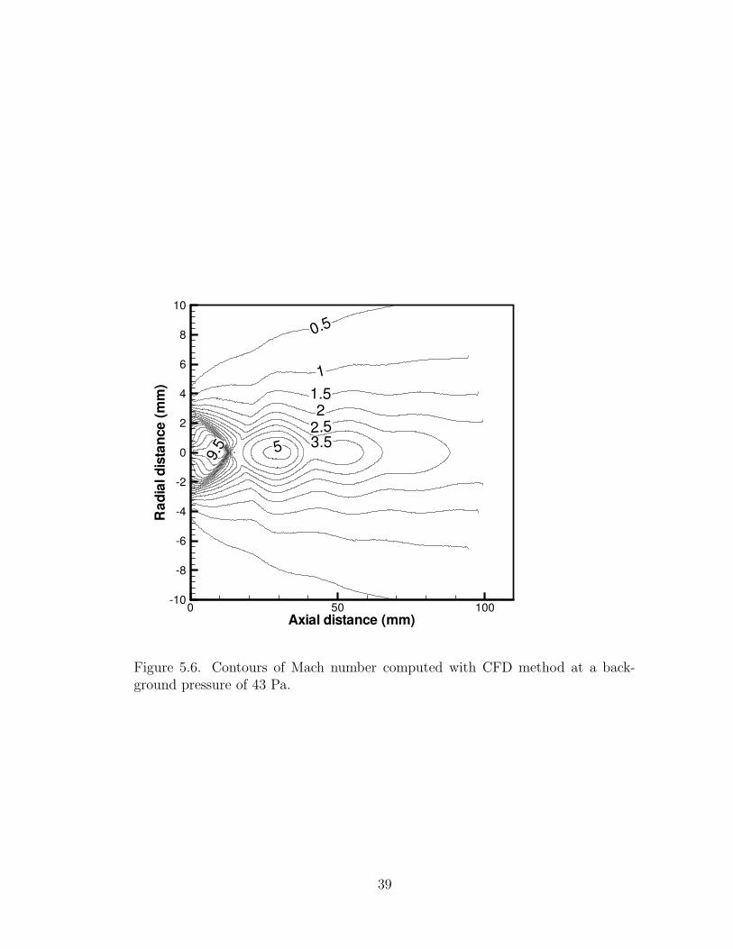
5.6 Contours of Mach number computed with CFD method at a back-ground pressure of 43 Pa. . . . . . . . . . . . . . . . . . . . . . . . 39

5.7 Pressure along the plume centerline computed with CFD methodat a background pressure of 43 Pa. . . . . . . . . . . . . . . . . . . 40

5.8 Comparison of number density along the plume centerline computedwith CFD method at a background pressure of 43 Pa using differentgrids . . . . . . . . . . . . . . . . . . . . . . . . . . . . . . . . . . . 41

5.9 Translational and rotational temperature along the plume center-line computed with CFD method at a background pressure of 43Pa. . . . . . . . . . . . . . . . . . . . . . . . . . . . . . . . . . . . 42

5.10 Comparison of contours of number density in molecules m−3 com-puted with the CFD method and DSMC method at a back pressureof 43 Pa.(contours multiplied by 1022) . . . . . . . . . . . . . . . . 44

5.11 Comparison of number density along the plume centerline computedwith the CFD method and DSMC method at a back pressure of 43Pa. . . . . . . . . . . . . . . . . . . . . . . . . . . . . . . . . . . . 45

5.12 Comparison of temperatures along the plume centerline computedwith the CFD method and DSMC method at a back pressure of 43Pa. . . . . . . . . . . . . . . . . . . . . . . . . . . . . . . . . . . . 46

ix

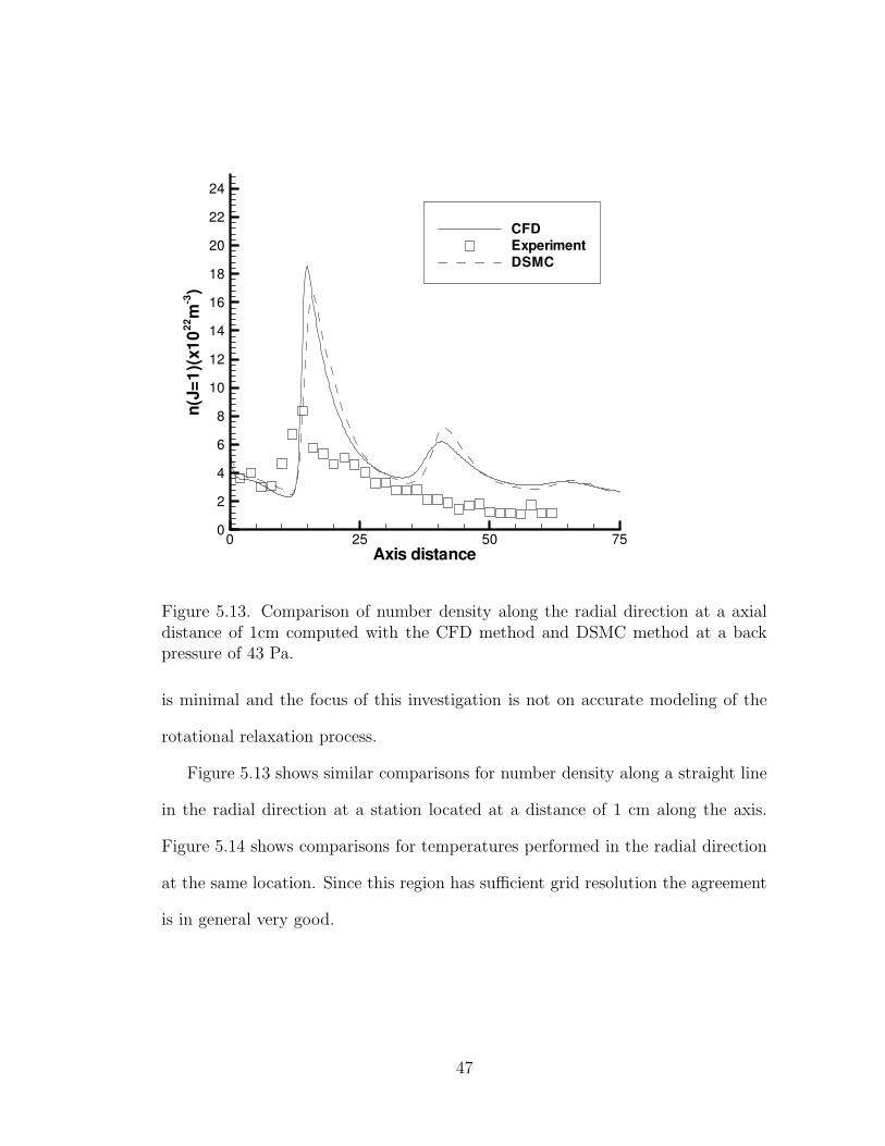
5.13 Comparison of number density along the radial direction at a ax-ial distance of 1cm computed with the CFD method and DSMCmethod at a back pressure of 43 Pa. . . . . . . . . . . . . . . . . . 47

5.14 Comparison of temperatures along the radial direction at a axial dis-tance of 1cm computed with the CFD method and DSMC methodat a back pressure of 43Pa . . . . . . . . . . . . . . . . . . . . . . 48

5.15 Comparison of measured and calculated data for the density of theJ = 1 state along the plume centerline at a back pressure of 43 Pa. 49

5.16 Comparison of number density along the plume centerline computedwith the CFD method and DSMC method at a back pressure of 10Pa. . . . . . . . . . . . . . . . . . . . . . . . . . . . . . . . . . . . 52


5.18 Comparison of number densities along the plume centerline com-puted with the CFD method and DSMC method at a back pressureof 1 Pa. . . . . . . . . . . . . . . . . . . . . . . . . . . . . . . . . . 54


6.1 Grid used for the CFD computations . . . . . . . . . . . . . . . . 646.2 Comparison of centerline pitot pressure measurements with of data

calculated from the simulations . . . . . . . . . . . . . . . . . . . 666.3 Centerline temperatures predicted by the simulation . . . . . . . . 676.4 Flow angle across the nozzle exit plane . . . . . . . . . . . . . . . 696.5 Comparison of contours of flow angles . . . . . . . . . . . . . . . . 706.6 Comparison of radial profiles of flow angles . . . . . . . . . . . . . 716.7 Centerline number density from numerical calculations and experi-

ments . . . . . . . . . . . . . . . . . . . . . . . . . . . . . . . . . . 736.8 Number density profiles along the radial direction at a distance of

0.27” from the nozzle exit plane . . . . . . . . . . . . . . . . . . . . 746.9 Number density profiles along the radial direction at a distance of

1.27” from the nozzle exit plane . . . . . . . . . . . . . . . . . . . . 756.10 Rotational temperature profiles along the radial direction at the

two axial stations . . . . . . . . . . . . . . . . . . . . . . . . . . . . 76

7.1 Comparison of breakdown parameters along the radial direction ata distance of 0.27” from the nozzle exit plane . . . . . . . . . . . . 84

7.2 Comparison of breakdown parameters along the radial direction ata distance of 1.27” from the nozzle exit plane . . . . . . . . . . . . 85

7.3 Grid used for the DSMC computations . . . . . . . . . . . . . . . 877.4 Number density profiles along the radial direction at a distance of

0.27” from the nozzle exit plane . . . . . . . . . . . . . . . . . . . . 88

x

7.5 Number density profiles along the radial direction at a distance of1.27” from the nozzle exit plane . . . . . . . . . . . . . . . . . . . . 90

7.6 Translational temperature profiles along the radial direction at atdistance of 0.27” from the nozzle exit plane . . . . . . . . . . . . . 91

7.7 Number density profiles along the radial direction at a distance of0.27” from the nozzle exit plane with an index of translational-equilibrium . . . . . . . . . . . . . . . . . . . . . . . . . . . . . . . 93

7.8 Temperature profiles along the radial direction at a distance of 0.27”from the nozzle exit plane . . . . . . . . . . . . . . . . . . . . . . . 94

7.9 Temperature profiles along the radial direction at a distance of 1.27”from the nozzle exit plane . . . . . . . . . . . . . . . . . . . . . . . 95

8.1 Grid used for the DSMC simulations . . . . . . . . . . . . . . . . . 1008.2 Number density profiles for simulations of CO2 expanding into vac-

uum . . . . . . . . . . . . . . . . . . . . . . . . . . . . . . . . . . . 1028.3 Number density profiles for simulations with ambient number den-

sity of 6.77e17 / m3 . . . . . . . . . . . . . . . . . . . . . . . . . . 1038.4 Comparison of measured and calculated data for the number density

in the back-flow region . . . . . . . . . . . . . . . . . . . . . . . . . 1048.5 Number density profiles for simulations with an ambient number

density of 1 × 1018m−3 . . . . . . . . . . . . . . . . . . . . . . . . . 1058.6 Comparison of number density profiles for simulations with an am-

bient number density of 1×1018m−3 and and ambient number den-sity of 6.77 × 1017m−3 . . . . . . . . . . . . . . . . . . . . . . . . . 106

8.7 Comparison of measured and calculated data for the mass flow ratein the back-flow region . . . . . . . . . . . . . . . . . . . . . . . . . 107

8.8 Contours of Chapman-Enskog parameter calculated based on theCFD solution . . . . . . . . . . . . . . . . . . . . . . . . . . . . . . 110

8.9 Comparison of contours of number density . . . . . . . . . . . . . 1118.10 Number density along a radial section at the exit plane . . . . . . . 1128.11 Comparison of measured and calculated data for the number density

in the back-flow region . . . . . . . . . . . . . . . . . . . . . . . . . 1138.12 Comparison of measured and calculated data for the mass flow rate

in the back-flow region . . . . . . . . . . . . . . . . . . . . . . . . . 114

xi

Chapter 1

Motivation and Background

This chapter presents the motivation behind this work and the scope of this work.

1.1 Introduction

Small rockets are used extensively for attitude control and other low thrust opera-

tions on trans-atmospheric vehicles and spacecraft. They are also used in satellites

for station keeping and various other operations. Low thrust electric thrusters and

a variety of chemical thrusters are being developed for these applications.

There a two main concerns involving the use of these thrusters. The first issue

is their efficiency. These nozzles are typically inefficient because of their small

size, which leads to losses due to viscous and non-equilibrium effects. Another

important issue is the effect of the exhaust plume impingement on the spacecraft.

Plume impingement on the vehicle surface may lead to unwanted heating of the

surface. The solar arrays and electronic devices may lose effectiveness under long

term exposure to rocket exhaust gases. These gases might contaminate the thermal

protection systems of trans-atmospheric vehicles. Impact of the plume on the

spacecraft might also produce unwanted torques or thrust losses. An accurate

assessment of these issues requires detailed understanding of the fluid dynamics and

kinetics of the nozzle and plume flow. With this in mind, several experimental and

1

numerical studies have been directed towards the prediction and characterization

of such flows.

Numerical investigations of all the issues involved in using these thrusters re-

quire accurate modeling of the complete nozzle plume system. Such investigations

are challenging because of the range of flow regimes involved. The flow regimes are

generally characterized by the Knudsen number, which can be defined as the ratio

of the mean free path to a characteristic length of the flow field. The Knudsen

number inside the nozzle is usually much less than one and this regime is referred

to as the continuum flow regime. As the flow expands the densities become lower

and lower and soon the Knudsen numbers are large enough for the flow to transi-

tion into the non-continuum regime. In the continuum regime the flow physics is

described by the Navier-Stokes formulation.

As the low-density effects become important there is considerable uncertainty

as to whether the continuum Navier-Stokes formulation adequately describes the

underlying physics. This had led researchers to take an alternative point of view

and simulate flows directly using Monte Carlo methods based on the molecular

theory of gases. The Direct Simulation Monte Carlo method developed by Bird

has been successfully used to simulate nozzle plume flows[1,2,3,4,5]. Although

Monte Carlo methods are efficient for very rarefied flows, they are prohibitively

expensive in the continuum regime. Thus from the point of view of performing

simulations of the complete nozzle plume system, Monte Carlo methods are accu-

rate and reliable but very expensive while the continuum Navier-Stokes equations

coupled with thermo-chemical non-equilibrium tools are solved rather efficiently

but of questionable validity in the very rarefied flow regimes.

Thus an approach using any one of these methods has limitations which would

2

prevent performing simulations of the complete system. This dissertation looks

at the possibility of using a combined approach and investigates the various steps

involved in pursuing such an approach.

1.2 Objectives and Scope of this work

Figure 1.1 shows a schematic of the nozzle plume system. The basic objective of

this dissertation is to investigate numerical approaches to studying this system and

develop an efficient and accurate method for performing such simulations.

A Navier Stokes solver that can be used to perform simulations of these systems

needs to be developed. Since these flows have complicated geometries and complex

flow gradients, an unstructured grid solver would be most efficient. The breakdown

of Navier-Stokes solvers would be analyzed in detail to understand the reason for

their failure and predict their failure accurately. The methodology needs to be

validated by comparing with experimental measurements. The focus of this work

is on developing and validating the methodology.

3

Figure 1.1. Schematic of the nozzle plume system

4

Chapter 2

Description of the combined approach

This chapter presents an outline of this work and a brief description of the rest of

the thesis.

2.1 Introduction

The objective of this study is to develop a method for performing numerical simu-

lations of a complete nozzle plume system for small rockets. Computer simulations

of the complete system from the inlet of the nozzle to the outer plume regions are

difficult to perform because of the wide range of Knudsen numbers involved. The

comparatively high-density flow inside the nozzle is most appropriately modeled

using a continuum based Computational Fluid Dynamics (CFD) approach. The

CFD method has physical and numerical limitations that prevent it from being

used for very rarefied flows. Since the outer plume and back-flow regions involve

very low densities, the direct simulation Monte Carlo (DSMC) method is used in

these regions. However, the DSMC method cannot be used for the full system, as it

is very expensive for simulating the comparatively high number densities inside the

nozzle. Thus an efficient and accurate numerical approach requires a combination

of these two methods. This thesis describes the development of such a combined

approach. The method is validated by applying it to the study of two systems for

5

which experimental results are available.

2.2 Description of methodology

The simplest combined approach involves splitting the domain into two and per-

forming two de-coupled simulations. The CFD method is used for the nozzle and

near plume regions while the DSMC method is used for the outer plume regions.

The CFD solution is used to prescribe boundary conditions for the DSMC code.

This combined approach involves three steps. The first step is developing and

implementing a Navier-Stokes solver for performing simulations of the nozzle and

near plume region. The next step is developing parameters for determining the

extent of the CFD domain by predicting the breakdown of the CFD method.

The third step is developing mechanisms for transferring information from the

CFD simulations to the DSMC simulations at the interface and performing DSMC

simulations. DSMC codes capable of performing simulations of the plume already

exist.

2.3 CFD Simulations

The CFD simulations are performed using an unstructured finite volume Navier-

Stokes solver. The CFD code is based on a cell centered finite volume formulation

that can be used on unstructured triangular or quadrilateral meshes. The equations

being solved are the Navier-Stokes equations expanded so as to include thermo-

chemical effects. The code takes into account rotational relaxation effects, vibra-

tional relaxation effects and chemical reactions. The details of the kinetics model

need to be implemented separately for each application. The convective fluxes

6

are calculated based on an upwinding method originally developed by MacCor-

mack and Candler[21] for structured grids. The implementation of the upwinding

method for unstructured grids is similar to the one described by Batina.[22] The

computation of gradients at each control volume is performed using Green-Gauss

integration around the control volume boundary.[23] A weighting process[24] is

used to improve accuracy so that in a regular triangular mesh made of equilateral

triangles the gradient is second order accurate. The code uses an explicit method

for time stepping and uses local time stepping to accelerate convergence.

2.4 Chapman-Enskog Parameter

Existing parameters for predicting continuum breakdown have two major limita-

tions. The value of the parameter at which breakdown is assumed to occur is

arbitrary. Also, they do not have a very strong theoretical basis. A new param-

eter is proposed in this thesis. It is based on the assumptions made during the

derivation of the Navier-Stokes equations from the Boltzmann equation. This pa-

rameter based on the Chapman-Enskog expansion is used to predict failure of the

Navier-Stokes solver.

2.5 DSMC Simulations

The DSMC method employs a large number of model particles to simulate the

behavior of the actual gas molecules. Due to the nature of the simulation method,

DSMC is capable of capturing nonequilibrium effects. The technique has been suc-

cessfully applied to model nozzle and plume flows expanding from small rockets[1,

2,3,4,5]. In this study DSMC simulations were performed using a parallel, opti-

7

mized implementation of the Direct Simulation Monte Carlo algorithm[17]. It is a

large system called ”MONACO” based on a DSMC algorithm formulated specif-

ically for workstation architectures. The DSMC simulations use results from the

CFD simulations as boundary conditions.

2.6 Outline of thesis

This section gives a brief outline of the rest of the thesis. Chapter three gives

a detailed description of the continuum code developed for this study. Chapter

four gives a brief description of the DSMC code used for the study. The DSMC

code has been used extensively before and is described in detail by Dietrich &

Boyd[17]. The first step in this study is the validation of the CFD code. The code

is validated by performing simulations of a hydrogen plume system. Experimental

studies on this system were conducted at Stanford University[19]. The results of the

validation study are presented in chapter five. The hydrogen system was found to

be unsuitable for demonstrating the advantages of using a combined methodology.

The experimental measurements of that system were not of sufficient resolution to

show a clear difference between the CFD computations and DSMC computations.

The next few chapters deal with the study of another experimental system

involving carbon di-oxide expansions into vacuum. This system was studied in de-

tail through experimental investigations conducted at Arnold Engineering Research

Center[9]. Tabel 2.1 shows the details of the two systems.

The nozzle and near plume simulations of a carbon dioxide system are described

in chapter six. Chapter seven looks at different continuum breakdown parameters.

Experimental measurements that agree with DSMC computations and disagree

8

Flow rate Area Ratio φ T0 Re Kn

Gas [Kg/m/s] [Degrees] [Kelvin]

H2 1 7.8 · 1012 7.2 9.2 0.0 0.0

CO2 3 6.5 · 1015 10.3 2.4 0.0 0.0

Table 2.1. The two systems investigated in this study.

with CFD computations are used to clearly demonstrate the breakdown of the

continuum approach. An analysis of the DSMC results is presented to investigate

the reasons behind the failure of the Navier-Stokes solver. Chapter eight presents

results of DSMC computations of the back-flow region. The last chapter presents

the conclusions of the study and suggestions for future work.

9

Chapter 3

Development of Unstructured grid solver

This chapter presents the underlying assumptions, the governing equations and the

numerical approach followed for developing the continuum code.

3.1 Introduction

The continuum code solves the set of coupled partial differential equations that

describes the dynamics of the flow field. The equation set is the Navier-Stokes

equations expanded to include finite rate relaxation processes. The formulation

assumes a generic problem, i.e. a gas mixture with rotational relaxation effects,

vibrational relaxation effects and chemical reactions.

The continuum formulation assumes that the Knudsen number, which can be

defined as the ratio of the mean free path associated with the flow to the character-

istic length scale of the body or the flow itself, is much less than one. In addition to

the equations of conservation of mass, momentum and energy, the shear stresses,

heat flux and diffusion velocities need to be expressed in terms of lower-order

macroscopic properties. These constitutive relations for the viscous stress tensor,

the heat flux vector, and the diffusion velocity of species in terms of gradients of

the flow are assumed to be linear. The thermal state of the gas is assumed to be

described by separate and independent temperatures. The energy in the transla-

10

tional modes is assumed to be characterized by a single temperature referred to

as the translational temperature. This assumption of translational equilibrium is

critical to the continuum formulation. A rotational temperature characterizes the

energy contained in the rotational mode. All vibrational modes are represented by

a single vibrational temperature. The vibrational mode is assumed to conform to

the harmonic oscillator description at all vibrational temperatures. This is accu-

rate at low vibrational levels, but becomes suspect at high vibrational temperatures

where the vibrational states may be non-harmonic. However the energy contained

in these states are negligible for the flowfields of interest in this study.

3.2 Mathematical formulation

The governing equations are basically the Navier-Stokes equations of gas dynam-

ics. To account for the non-equilibrium processes considered, a partial differential

equation is added for each energy mode considered. These equations are described

in detail in this section.

3.2.1 Conservation equations

The equations are presented in their Cartesian tensor notation for simplicity, al-

though two-dimensional axisymmetric equations are used in this study. The con-

servation of mass is replaced by a species equation for each individual species due

to chemical nonequilibrium. For a gas made up of ns species there would be ns

species continuity equations. The species continuity equation, which states the

conservation of mass, for any species i in the gas mixture is given by

∂ρi

∂t+

∂(ρiuk + jik)

∂xk= ωi, (3.1)

11

where ρi is the density of species i , uk is the velocity component in the k direction

and ji,k is the diffusive mass flux of species i in the k direction. ωi is the source term

for species i and it represents the rate of production of species i due to chemical

reactions.

The mass averaged momentum equation, which gives the conservation of mo-

mentum in a gas mixture, is given by

∂ρuj

∂t+

∂(ρujuk + τjk + pδjk)

∂xk= 0. (3.2)

Here ρ is the density of the flow, while ui, uj, uk are velocity components in the i,

j, and k directions, τi,j is a component of the shear stress tensor, p is pressure and

δj,k is the delta function.

Two additional energy equations are introduced to account for thermal nonequi-

librium processes i.e. the relaxation of vibrational and rotational degrees of free-

dom. The conservation of vibrational energy within a diatomic species is as follows

∂Ev

∂t+

∂(ukEv + qvk)

∂xk= ωv, (3.3)

where Ev is the energy in the vibrational mode, qvk is the heat flux associated

with the vibrational mode in the k direction, uk is the velocity component in the

k direction and ωv is the vibrational source term.

The conservation of rotational energy is expressed

∂Er

∂t+

∂(ukEr + qrk)

∂xk= ωr, (3.4)

where where Er is the energy in the rotational mode, qrk is the heat flux associated

with the rotational mode in the k direction and ωr is the rotational source term.

Finally the conservation of total energy is stated by

∂E

∂t+

∂((E + p)uk + qkujτjk)

∂xk= 0, (3.5)

12

where E is the total energy, and qk is the total heat flux in the k direction, while

ui, uj, uk are velocity components in the i, j, and k directions, τi,j is the component

of the shear stress tensor and p is pressure.

3.2.2 Equations of state

The equations of state used to calculate the non-conserved quantities from the

conserved quantities are presented now. The equation of state for pressure of the

gas mixture is given by

p = ρRT, (3.6)

where ρ is the density and R is the gas constant and T is the temperature.

The total energy per unit volume, E, is made up of the various modes of internal

energy, i.e. translational, rotational, vibrational, the kinetic energy of the flow and

the energy arising from the formation of the species. Therefore the total energy

per unit volume for a gas with ns species is given by

E = CvρT + Ev + Er +1

2ρ(u2 + v2) +

ns∑

i=1

ρih0i (3.7)

Here Cv is the specific heat at constant volume, T is the temperature, Ev and Er

represent the energy contained in the vibrational and rotational modes, ρ is the

density of the gas and u and v are the velocity components in the x and y direction

and h0i is the heat of formation of species i.

The vibrational energy in any diatomic species i is expressed by

Evi = ρiR

Mi

θvi

e(θviTv

) − 1), (3.8)

where θvi is the characteristic temperature for vibration, Mi is molecular weight of

species i and Tv is the vibrational temperature. The rotational energy is represented

13

by

Eri = ρiR

MiTr, (3.9)

where Tr is the rotational temperature. The vibrational temperature of the in-

dividual species is determined by inverting the expression for vibrational energy

contained in a simple harmonic oscillator at the temperature. This inversion is done

using an iterative procedure using Newton’s method. The rotational temperature

is obtained from the Eq.(3.9) .

3.2.3 Shear stresses, Heat fluxes and Diffusion velocities

In the Navier Stokes formulation the diffusive fluxes are linearly related to the

gradients of the associated flow quantities. Thus from the Newtonian fluid as-

sumption the shear stress tensor can be related to the velocity gradient tensor by

the expression

τij = −µ(∂ui

∂xj+

∂uj

∂xi) − λ

∂uk

∂xkδi,j (3.10)

with the Stokes hypothesis

λ =−2

3µ. (3.11)

Here τi,j is the component of the shear stress tensor, ui is the component of velocity

in the i direction and δi,j is delta function. µ is the coefficient of viscosity and is

calculated for each species using the viscosity model for a reacting gas developed

by Blottner[6]. The model uses a curve fit with three constants to give

µs = 0.1exp[(AslnT + Bs)lnT + Cs], (3.12)

in kg/m s, as a function of temperature T. The constants, As, Bs and Cs need to

be specified for the each gas species. For some of the applications presented in this

thesis this model has been replaced by a model developed for DSMC methods where

14

the dependence of µ with temperature is specified. These models are described in

the subsequent chapters. The total viscosity of the gas is then calculated using

Wilke’s semi-empirical mixing rule[7].

Fourier’s law of heat conduction gives the heat flux vector, qφ associated with

energy mode φ to the gradient of temperature Tφ

qj = −κφ∂Tφ

∂xj

. (3.13)

Here κφ is the thermal conductivity associated with Tφ. The conductivity of the

rotational and vibrational temperatures for each species may be derived from the

Eucken relation[8]. With this formulation it is assumed that the transport of

translational energy involves a correlation with the velocity, but the transport of

internal energy (rotational and vibrational) involves no correlation with velocity.

The thermal conductivity for translational energy, κt, is

κt =5

2µCvt

, (3.14)

where µ is the coefficient of viscosity and Cvtis the specific heat at constant

volume for translational energy. The total thermal conductivity of the gas is then

calculated using Wilke’s semi-empirical mixing rule[7].

Similarly Ficks law of diffusion give the diffusive mass fluxes for species s as

ρsvsj = −ρDs∂cs

∂xj, (3.15)

where ρs is the density of the species, vsj is the diffusion velocity, and cs is the

mass fraction of the species s . The diffusion coefficient Ds is derived by assuming

a constant Lewis number, Le which by definition is given by

Le =Dρcp

κ, (3.16)

15

where ρ is density, Cp specific heat at constant volume and κ is the coefficient of

thermal conductivity.

3.2.4 Energy exchange mechanisms

Vibration translation (V-T) energy exchange is the process by which energy is ex-

changed between the vibrational and translational modes. This process appears as

source terms in the conservation equation for the vibrational energy mode. The

Landau-Teller form of vibrational relaxation represents a V-T energy transfer and

describes how the system of oscillators approaches its equilibrium state. These en-

ergy transfers appear as source terms in the equations described above. The source

terms in the vibrational energy equation for any molecular species i is assumed to

be

wvi =E∗

vi − Evi

τvi(3.17)

, where Evi is vibrational energy per unit volume and τvi is the vibrational re-

laxation time. E∗

vi is the vibrational energy evaluated at the local translational

temperature. The source terms in the rotational energy equation are similar to

those in the vibrational energy equation. The rotation-translation energy mecha-

nism would be

wri =E∗

ri − Eri

τri, (3.18)

where Eri is rotational energy per unit volume and τri is the rotational relaxation

time. Similarly E∗

ri is the rotational energy evaluated at the local translational

temperature.

16

3.3 Numerical method

Traditionally structured methods that rely on regular array of quadrilateral cells

have been used to solve such problems. Recently, unstructured grid methods have

emerged as a viable alternative to discretizing complex geometries. These meth-

ods provide greater flexibility for discretizing complex domains and also enable

straightforward implementation of adaptive meshing techniques. Since these flows

have complicated gradients that need to be captured accurately, the continuum

method is formulated for unstructured grids. Since the DSMC code also uses un-

structured grids this simplifies the division of the domain between the two methods

and also facilitates communication between the two methods.

The conservation law form of the two dimensional (or axi-symmetric) Navier-

Stokes equations, with n chemical species including chemical and thermal nonequi-

librium (m separate vibrational modes) processes, in the Cartesian coordinates can

be written as

∂U

∂t+

∂(F + Fv)

∂x+

∂(G + Gv)

∂y= W, (3.19)

, where U is the state vector, F and G are the convective flux vectors, Fv and Gv

are the diffusive flux vectors, and W is the source term vector. The state vector

U, the convective flux vectors F and G, are defined as follows:

17

U =

ρ1

ρ2

...

ρn

ρu

ρv

Ev1

Ev2

...

Evm

Er

E

, F =

ρ1u

ρ2u

...

ρnu

ρu2 + p

ρuv

uEv1

uEv2

...

uEvm

uEr

u(E + p)

, G =

ρ1v

ρ2v

...

ρnv

ρuv

ρv2 + p

vEv1

vEv2

...

vEvm

vEr

u(E + p)

.

Fv =

1x

2x

...

nx

τxx

τyx

qv1x

qv2x

...

qvmx

qrx

uτxx + vτyx + qx

, Gv =

1y

2y

...

ny

τsy

τyy

qv1y

qv2y

...

qvmy

qry

vτyy + uτxy + qy

, W =

ω1

ω2

...

ωn

0

0

ωv1

ωv2

...

ωvm

ωr

0

18

are the viscous (diffusive) fluxes Fv and Gv, and the source vector, W.

Here the flux vector is split into an inviscid flux vector and a viscous flux vector.

In the integral form for a control volume V(t) with boundary S(t) the governing

equations are given by

∂

∂t

∫

V (t)

Wdv +∮

S(t)

(F~i − G~i) · ~ndl +∮

S(t)

(Fv~i − Gv

~i) · ~ndl = 0. (3.20)

Since the domain is subdivided into polygonal elements the semi-discrete form of

this equation is given by

Ωs∂W

∂t= −

n∑

s=1

Hs∆ls,−−n

∑

s=1

Hvs∆ls, (3.21)

where Ωs denotes the volume of the cell, Hs is a numerical approximation to the

normal convective flux crossing a face s with side length ∆ls and n is the number

of sides of the polygon. Hvsis the corresponding viscous flux. Hs and Hvs

can be

obtained by rotating the flux terms in Eq. 3.10 as follows

H = F~i − G~i. (3.22)

The expression for the flux Fs at the interface can be calculated by a number

of upwind methods. It should noted that it is now a one dimensional problem

where the flux normal to the face is being evaluated. In this implementation, it

is performed using the flux-vector splitting proposed by MacCormack, which is

briefly explained here.

The computation of the inviscid flux terms are based on an upwinding tech-

nique. Upwinding techniques model the underlying physics better than more con-

ventional centered methods. The upwinding method used was developed for struc-

tured grids by MacCormack and Chandler[21]. They successfully applied it to the

19

investigation of numerous hypersonic flows. The details of their method are de-

scribed in Chandler’s thesis[8]. The implementation of the upwinding method for

unstructured grids is similar to the one described by Batina.[22]

Evaulation of the inviscid part involves calculating the term∮

S(t)

(F~i − G~i) · ~ndl

in the previous equation.

The convective flux is assumed to have two parts F = F+ +F−, where F+ is the

flux associated with the right running waves, and F− with the left running waves.

The splitting of the flux vector is not unique and many possibilities for splitting

exist. In this implementation we use the MacCormack-Chandler scheme which is a

variation of the Steger-Warming scheme. The splitting is based on an approximate

solution of the Riemann problem in one dimension. In the Steger Warming type

flux vector splitting, we make use of the fact that the convective flux vector is

homogenous of degree one in U, i.e., F=AU, where A is the Jacobean of F with

respect to U. The matrix A can be diagonalized using similarity transformations

such that A = S−1C−1A ΛCAS. Chandler describes these matrices S, CA , S−1, and

C−1A in detail[8]. A can now be split into two parts depending on the sign of the

eigenvalues

A+ = S−1C−1A Λ+CAS (3.23)

A− = S−1C−1A Λ−CAS. (3.24)

Then the split fluxes have the form F+ = A+U and F− = A−U .

Fs = AL+R

2

+ UL + AL+R

2

−UR. (3.25)

The same flow state [ (L+R)2

] is used to evaluate the positive and negative Ja-

cobians. This contrasts with the Steger-Warming scheme, in which the Jacobians

are upwinded. MacCormack and Candler[34] proved that this simple modification

20

results in a significant improvement in accuracy. This method was developed for

application in boundary layers and leads to numerical instability when applied to

strong shock waves. In such regions the scheme reverts back to the Steger-Warming

scheme in a smooth manner with a pressure based switch described by Chandler[8].

For a higher order extension, the piecewise constant solution is replaced by a

linear one, according to the relation :

Q(x, y)A = Q(x0, y0)A + ΦA∇QA · ∆r with Φ ∈ [0, 1], (3.26)

where ∇QA represents the constant gradient of the solution on each cell and ∆r the

local coordinates of a point within the element. In this expression, the parameter

ΦA is a slope limiter used to avoid a new maxima or minima. The gradients used

is the same as the ones used for the viscous terms and they are described later.

The computation of the viscous terms requires the gradients of flow properties at

each cell. The computation of gradients at each control volume is performed using

Green-Gauss integration around the control volume boundary.[23] A weighting

process[24] is used to improve accuracy so that in a regular triangular mesh made

of equilateral triangles the gradient is second order accurate.

21

Chapter 4

Description of Monaco

This chapter gives a brief description of the DSMC code used for these simulations.

4.1 Introduction

The direct simulation Monte Carlo (DSMC) method is a numerical technique that

uses particles for simulating fluid flow. The DSMC method has been successfully

applied to a wide variety of rarefied gas flows. The method is based on the as-

sumption that particle motion and collisions can be uncoupled for a time step

smaller than the mean free path time between collisions. A brief description of

the algorithm involves three steps. First, new particles are generated at the inflow

boundaries and all particles are moved in the computational domain disregarding

collisions with other particles but including interactions with wall boundaries. Each

particle has its own position, mass, velocity and internal energy. The grid used

has cell dimensions of the order of local mean free path in order to group possible

collision partners in each cell. In the second step, a statistical method is applied

to each group achieving typical collisions appropriate for the chosen time step.

The models used for collisions and energy exchange are mostly phenomenological.

Finally, flow properties in each cell are sampled if the calculation has reached a

steady state.

22

4.2 Monaco

The Monaco software is split into two parts: the MONACO library, a set of subrou-

tines for modeling the flow physics and the MONACO kernel, a set of subroutines

for memory management and parallelization. The MONACO library is a collection

of subroutines written in FORTRAN. These routines handle the flow physics in a

single cell. The computation of particle collisions and generation of inflow particles

are handled by these subroutines. Some of these sub-routines dealing with collision

models and relaxation models need to be changed for different applications.

The MONACO kernel is written is C and handles the grid structure and particle

management. Since this part of MONACO is completely uncoupled from the flow

physics, this does not need to be changed when physical models are changed in

the MONACO library. The MONACO kernel is based on unstructured triangular

or quadrilateral grids. This allows for great flexibility in dealing with flows with

complicated geometry and gradients. Since the CFD code also uses unstructured

grids, it was straightforward to split the domain into a CFD region and a DSMC

region. It also allowed for simulations using both codes to be performed on the

same grids for comparison.

Particle properties are obtained from a specified distribution function at the

inlet of the computational domain. Particles are paired for possible collisions.

The probability of a collision is a function of the collision cross section and the

densities of the species. Various techniques can be used to determine if a pair

of particles collide. These include the Time Counter method,[18] the No Time

Counter method,[18] and a scheme developed by Baganoff and McDonald.[33] The

macroscopic collision rate must be reproduced by the instantaneous probabilities of

23

collision. Each technique accomplishes this. However, the Baganoff and McDonald

scheme is chosen for the present implemenation, because it is more computationally

efficient.

The collision dynamics are performed in the center of mass reference frame.

Particles may exchange translational as well as internal energy during a collision.

Models for exchanging internal energy include rotational[30] and vibrational[31,32]

energy. However, the present study only considers translational energy transfer,

because the propellent gas is monatomic xenon. The cross sections are functions

of collisional energy and depend on the mode of energy to be transferred.

In order to update the particles’ positions, a time ∆t must be specified. There-

fore, an algorithmic approach in which a time step is used for each iteration is

employed. This time step should be a fraction of the mean time between collisions

in order to capture the collisional effects in the flow properly.

The collisions serve to alter the distribution function. The density, momentum,

and temperature of the flow are derived from the zero, first, and second moments

of the velocity distribution function respectively. Sampling the computational par-

ticles, which is essentially averaging, gives these macroscopic flow properties. For

steady flows, the sampling can be extended for a large number of time steps in

order to reduce statistical error. It has been shown that this error is a function of

the number of particles in a cell and the number of sampling time steps.[29] For

unsteady flows, care must be taken to obtain realistic averages.

The geometry may be zero dimensional to fully three dimensional. Zero dimen-

sional simulations allow physical modeling and collisional behavior to be examined

while the movement is unnecessary. A three dimensional implementation of DSMC

is described in Ref.[28]. Fully three dimensional modeling requires considerably

24

more memory and execution time than two dimensional modeling. Not only is

more cell information needed, but also more particles must be employed. These

two requirements lead to substantially longer simulations. Therefore, the present

study assumes symmetry in the azimuthal direction and uses cylindrical coordi-

nates. Axisymmetric flows can be represented by a two dimensional grid, but the

movement routine uses all three velocity components. The geometry is assumed

to be a single azimuthal plane. Particles are moved in all three directions and are

then mapped back into this plane.

Particles store their positions and move through the cells according to their

velocities. In the present implementation, particles which reach cell boundaries

are passed to the neighboring cell. The boundaries of each cell are defined as

either walls, symmetry lines, inflows, outflows, or cells which share an edge (called

neighbors). Walls may be fully specular, fully diffuse, or a combination of the two.

Fully specular walls simply reflect the particle back into the simulation without

altering properties other than the velocity vector. Fully diffuse walls accommodate

the particles to the wall temperature and sample properties from a distribution

before returning them to the cell. It is often necessary to treat some of the collisions

between particles and walls as specular and the rest as diffuse.[18] Symmetry lines

essentially act as specular reflection walls. Particles reaching inflow or outflow

boundaries are removed from the simulation. It is often important to include

the facility background pressure in simulations when comparing with experimental

data. The present application is a good example. To represent this effect, particles

can be introduced at the boundaries at a specified density and temperature, but

this may take a considerable amount of time to reach a steady state. Another

approach is to impose ambient conditions uniformly in the cells at the start of

25

a simulation and allow them to move through the domain. However, this may

require substantially more particles than are desired for a simulation. A scheme

which imposes a background density and temperature is described in Chapter 4.

Temporary particles are created in the cells for possible collisions, but they are not

tracked by the code.

26

Chapter 5

Hydrogen plume flow

The first step towards developing the method described for performing simulations

of a complete nozzle plume system is the development and validation of a contin-

uum code. This chapter describes the validation of the continuum code described

in chapter three. The code is applied to study hydrogen plume flows in arc-jet

experiments conducted at Stanford University[19]. First, the results obtained from

nozzle and plume flow simulations using the continuum code are compared with

experimental measurements. Detailed comparisons are also made of the plume flow

results with computational results obtained from DSMC simulations. Finally the

extent of validity of the continuum approach is investigated by performing a few

simulations of the hydrogen gas expanding into very low background pressures.

5.1 Introduction

Low power hydrogen arc-jet propulsion devices are used in spacecraft for orbit

transfer and station-keeping maneuvers. The thrust efficiencies achieved with these

rockets have only reached about 30%. Many of the factors that cause this rela-

tively low efficiency are concerned with the fluid mechanics and chemical kinetics

of hydrogen. An experimental investigation employing Raman scattering to obtain

number density and rotational temperature was performed at Stanford University

27

to examine these effects at a fundamental level. Boyd has performed detailed com-

parisons of these measurements with results obtained from DSMC simulations[19].

The flow regime varies from low Knudsen numbers inside the nozzle to very high

Knudsen numbers in the plume. These studies found that the flow is dominated

by effects of thermal relaxation and by viscosity in the nozzle boundary layer.

The flow conditions, availability of experimental measurements, and results from

previous DSMC simulations made this system a good candidate for testing and

validating the CFD code.

First, the nozzle flow simulations are performed. The domain starts at the

inlet of the nozzle and ends a short distance away from the exit plane. The results

obtained are validated with experimental measurements. A separate simulation of

the near plume region is performed next. For this simulation the domain starts

with the exit plane of the nozzle and extends into the near plume region. For these

simulations the background pressure was maintained at 43Pa in the experimental

facility. Detailed comparisons are made with results obtained from a DSMC code

to assess the agreement between the two approaches. The computational results

are compared with experimental measurements of number density and rotational

temperature in the plume. After validating the CFD code, simulations of hydrogen

expanding into very low background pressures are performed using the CFD code.

The results obtained are compared with DSMC results to study the breakdown of

the continuum approach. These flows have relatively high Knudsen numbers and

test the validity of the continuum approach.

The finite volume Navier-Stokes solver can be used with unstructured triangular

or quadrilateral meshes. The use of unstructured grids allows for various solution

adaptive gridding techniques. In the present study, an initial solution for the flow

28

field is obtained using a coarse grid. Grid refinement is then performed using the

coarse grid solution. The solution is then transferred from the coarse grid to the

fine grid. Although efficient use of unstructured grids requires further study of

various solution adaptive strategies, the transfer of the coarse grid solution to the

fine grid greatly reduces the time required for the final solution. Grid refinement

requires an estimation of minimum cell sizes needed to capture the flow features

accurately. Different methods can be used to estimate this cell size. Initially a

method based on the gradient of number density, calculated from the coarse grid

solution, was tried. This method ran into difficulties because the gradients were

not smooth enough for the grid generator. This was avoided by generating a series

of grids with cell sizes in multiples of the mean free path values obtained from the

coarse grid simulation.

5.2 Experimental Details

The experiments were conducted in the vacuum facility at Stanford University.[19]

The flow under consideration is the low-density expansion of molecular hydrogen

from a 1kW-class NASA hydrogen arc-jet thruster. The nozzle has a throat diam-

eter of 0.64 mm with a 200 degree half-angle, and an exit-to-throat area ratio of

225:1. The mass flow rate through the thruster is 14.1 mg/s and the stagnation

temperature is 300K. The conditions chosen for examination represent a cold flow

configuration in which the arc is not ignited. These conditions correspond to a

Knudsen number of the order of 0.01 at the nozzle exit.

The flow is assumed to expand into a background pressure of 43 Pa. The over-

all experimental configuration is shown schematically in figure 5.1. Of particular

29

Figure 5.1. Schematic of the experimental system

interest is the position of the vacuum pumps with respect to the expanding flow.

The location of the pumps will clearly give a non-symmetric pressure distribution.

It is difficult to perform an exact simulation of the chamber residual pressure since

it is not distributed homogeneously throughout the chamber.

The experimental measurements employ spontaneous Raman scattering. Ra-

man scattering is an inelastic, linear two-photon scattering process. An incident

photon scatters off an H2 molecule causing a change in the molecular quantum

state and a corresponding change in the energy of the scattered photon. The num-

ber of scattered photons is linearly proportional to the number of incident photons

and the density of the scattering species. Density is determined by the absolute

intensity of all transitions combined in conjunction with the signal from a reference

30

cell. For the present comparisons the experimental data, taken along the plume

centerline, give the density of the J=1 rotational state. The J=1 rotational state

was chosen in order to facilitate high spatial resolution. Each experimental data

point is obtained over a volume that is 4mm in length axially and 0.1mm in the

radial direction. The relative intensity of the various transitions can be used to

determine a rotational temperature, assuming partial thermodynamic equilibrium

exists among the rotational states. Experimental data is taken along the exit plane

and the plume centerline.

5.3 CFD Code

A description of the Navier-Stokes solver is presented in chapter three. A kinetics

model and the boundary conditions need to be implemented before the code is

applied to a specific study. This section describes the details of the kinetics model

and the boundary conditions implemented for this particular application.

5.3.1 Kinetics

The problem under consideration is a single species flow of molecular hydrogen.

The stagnation temperature of the flow is 300K. Since the temperatures involved

are low, the vibrational mode is assumed to be frozen and dissociation of hydrogen

is not important. Model parameters for the rotational relaxation rate and the

viscosity coefficient of molecular hydrogen must be provided as inputs to the code.

The kinetics scheme implemented in the code is based on a model developed for

DSMC simulations of such flows by Boyd et al[19]. The viscosity model used has a

temperature coefficient of 0.67 and gives an excellent fit to measured data[19]. For

31

the CFD simulations, the energy exchange rate between the translational mode

and the rotational mode is given by

Qt−r = ρe∗r(T ) − er

τr(5.1)

where e∗r(T ) is the rotational energy per unit mass evaluated at the local trans-

lational temperature and τr is the relaxation time. For these simulations, the

relaxation time is based on the form

τr = τc ∗ Zr (5.2)

where τc in the inverse of the molecular collision rate. τc is calculated using

τc = πµ/(4p), (5.3)

where µ is the coefficient of viscosity and p is the pressure[20]. Zr is the rotational

collision number for hydrogen which is given by[19]

Zr = 10480/T ω (5.4)

ω, the temperature coefficient of viscosity, is assumed to be 0.67.

5.3.2 Boundary Conditions

The two separate simulations require slightly different boundary conditions. For

the nozzle simulations, the inlet boundary conditions are subsonic and exit bound-

ary conditions are supersonic. The nozzle wall is assumed to be isothermal.

For the plume simulations, the solution domain starts at the exit plane of the

nozzle. There are three types of boundaries corresponding to the exit plane of

the nozzle, outflow boundary and the axis of the plume. The inlet is supersonic

and so all the conditions are prescribed at the beginning of the simulation and not

32

changed. These inlet conditions, which correspond to the conditions at the nozzle

exit, are obtained from a DSMC simulation of the nozzle flow. De-coupling the

nozzle flow simulations from the plume simulations saves a great deal of computa-

tional expense. The decoupling approach has been successfully applied in previous

investigations using the DSMC technique by Boyd et al[25] and Penko et al[26] .

The outflow boundary condition depends on the Mach number of the flow

normal to the domain exit plane. If the flow is supersonic all the flow properties

are extrapolated from the flow domain. If the flow is subsonic the pressure at the

eexit is assumed to correspond to the background pressure of the flow and all other

flow properties are extrapolated or calculated. The axis is assumed to be a line of

symmetry. The domain is made large enough so as to minimize the effect of the

exit boundary conditions on the flow near the nozzle exit.

5.4 Nozzle Simulation Results

First, the CFD code is validated for nozzle simulations. The CFD results obtained

are compared with experimental measurements. Figure 5.2 shows the comparison

of number density of the J=1 rotational state of hydrogen in the nozzle exit plane.

The number density of the excited state is calculated using the equilibrium ex-

pression along with the number density and the rotational temperature obtained

from the simulation. There is reasonably good agreement between numerical and

experimental results. Figure 5.3 shows the rotational temperature across the noz-

zle exit plane. The agreement between the numerical results and the experimental

measurements is very good.

To check the sensitivity of the solution to the resolution of the grid, the simu-

33

-4 -2 0 2 4Radial distance (in mm )

0

1

2

3

4

5

6

Num

berd

ensi

tyof

J=1

exci

ted

stat

eof

H2

(x10

22/m

3 )

Figure 5.2. Comparison of measured and calculated data for the density of the(J=1) rotational state across the nozzle exit plane

34

-6 -5 -4 -3 -2 -1 0 1 2 3 4 5 6Radial Distance (in mm)

0

20

40

60

80

100

120

140

160

180

200

220

240

260

280

300

Rot

atio

nalT

empe

ratu

re

Figure 5.3. Comparison of measured and calculated data for the rotational tem-perature across the nozzle exit plane

35

0 1 2 3 4 5Radial Distance (in mm)

0

500

1000

1500

2000

2500

3000

Vel

ocity

inth

eax

iald

irect

ion

0

50

100

150

200

250

300

Tra

nsla

tiona

lTem

pera

ture

Fine Grid - tCoarse Grid - tFine Grid - uCoarse Grid - u

Figure 5.4. Comparison of axial velocity and translational temperature along thenozzle exit plane computed with CFD method using different grids

36

lations are repeated on a finer grid. The coarse grid has around 10,000 cells while

the fine grid has about 36,000 triangles. There was no appreciable difference be-

tween results from the two simulations. Figure 5.4 shows the comparison of the

velocity in the axial direction and the translational temperature along the axis

obtained using different grids. Thus it can be concluded that grid resolution is not

an important issue for these flows.

5.5 Plume Simulation Flow field results

Plume flow field properties predicted by the CFD code are presented in this section.

The flow domain begins at the exit plane of the nozzle and extends to about 10

cm in the axial direction and 3 cm in the radial direction. Contours of the number

density in particles per m3 obtained for this condition are shown in Figure 5.5.

The finite back pressure creates a thin jet of diameter about 1 cm. The flow is

highly overexpanded and shows a very complicated flow pattern involving Mach

disks and shock waves. Contours of Mach number are shown in Figure 5.6. The

supersonic portion of the flow is restricted to a narrow core of diameter 8mm and

is enveloped by a barrel shaped shock structure. There is a region of high density

between the shock and the plume boundary where the flow is decelerated rapidly.

The flow shows a repetitive pattern of expansion followed by compression, which

decreases in strength as we go downstream. The pressure distribution along the

axis, shown in Figure 5.7, clearly shows the extent of overexpansion and the repet-

itive pattern of expansion and compression. The amplitudes of these compressions

are found to depend very highly on the cell size. Figure 5.8 shows the number den-

sity along the plume centerline obtained using different grids. Results using three

37

0 25 50 75 100Axial distance (mm)

-10

-8

-6

-4

-2

0

2

4

6

8

10

Rad

iald

ista

nce

(mm

)

234 54

1 1.5

Figure 5.5. Contours of number density in molecules m−3 computed with CFDmethod at a background pressure of 43 Pa.(contours multiplied by 1022)

38

0 50 100Axial distance (mm)

-10

-8

-6

-4

-2

0

2

4

6

8

10

Rad

iald

ista

nce

(mm

)

0.5

11.52

2.53.559.

5

Figure 5.6. Contours of Mach number computed with CFD method at a back-ground pressure of 43 Pa.

39


0

25

50

75

100

125

150

175

200

Pre

ssur

e(P

a)

Figure 5.7. Pressure along the plume centerline computed with CFD method at abackground pressure of 43 Pa.

40

0 50 100Axial distance (mm)

0

5

10

15

20

25N

umbe

rden

sity

(x10

22m

-3)

Grid 1 - 20,000 cellsGrid 2 - 45,000 cellsGrid 3 - 65,000 cells

Figure 5.8. Comparison of number density along the plume centerline computedwith CFD method at a background pressure of 43 Pa using different grids

grids are shown in the figure. The coarsest grid has 20,000 cells. The solution

obtained using this grid is used as a basis for generating other grids. The other

grids have 45000 and 65000 triangles respectively. As the cell size is decreased the

amplitude of the waves increases. Due to efficiency considerations, only the first

compression is captured in a grid independent manner. In this region the solutions

from the two fine grids coincide. Thus it can be concluded that in this region

the solution is more or less free of grid effects. Further refinement, even in other

regions does not effect the solution in this region. The complex nature of the flow

and the need for extremely small cells to capture the flow accurately underlines

the advantages of flexible gridding techniques available with unstructured grids.

41


0

25

50

75

100

125

150

175

200

225

250

Tem

pera

ture

(K)

TranslationalRotational

Figure 5.9. Translational and rotational temperature along the plume centerlinecomputed with CFD method at a background pressure of 43 Pa.

42

There is a high degree of rotational non-equilibrium in the flow. Figure 5.9

shows the rotational and translational temperatures along the plume centerline.

Due to the rapid expansion in the nozzle the translational temperature is much

lower than the rotational temperature at the exit of the nozzle. Inside the plume

near the axis, the translational temperature rises due to a series of rapid compres-

sion processes and becomes higher than the rotational temperature. Far down-

stream both temperatures approach equilibrium as the strengths of these compres-

sions decreases.

5.6 Comparison with DSMC Results

This section presents the results obtained from the DSMC simulations and their

comparison with the results from the CFD computation. The DSMC code used

is described in chapter four. The code is used with unstructured triangular grids.

The DSMC simulations are carried out using the same grid as the CFD simulations.

The grid consists of about 42,000 triangles. The cell sizes in the region near the

nozzle exit are about three times the mean free path. The CFD simulations are

performed on a SGI workstation and take around 30 hours of CPU time to converge.

The DSMC computations are carried out on an IBM SP2. The code is run in the

parallel mode using 4 processors for about 12 hours. For these simulations there

were about one million particles in the simulation.

The exit plane boundary conditions for the DSMC simulation requires knowl-

edge of both pressure and temperature. The pressure is assumed to be the residual

chamber pressure of 43 Pa. The temperature cannot be calculated a priori and

there are no experimental measurements available. Thus for the purpose of these

43

0 20 40 60 80 100Axial distance (mm)

-10

-8

-6

-4

-2

0

2

4

6

8

10R

adia

ldis

tanc

e(m

m)

2

3

4

4

5

3

2

34

CFD Solution

DSMC Solution

Figure 5.10. Comparison of contours of number density in molecules m−3computed with the CFD method and DSMC method at a back pressure of 43Pa.(contours multiplied by 1022)

simulations the exit plane temperature are taken from the CFD simulations. Pre-

vious results had indicated that the temperature at the exit plane boundary does

not effect the flow near the nozzle exit, which is the primary region of interest.

First, number density contours are compared to assess the overall agreement.

From Figure 5.10 it can be concluded that both methods give very similar results.

The flow properties along the axis are then compared in detail. Figure 5.11 shows

the number density profiles along the plume centerline in the axial direction. There

is very good agreement between the two solutions for about 4 cm in the axial

direction. The amplitude of the secondary compression region is under-predicted

44


0

2

4

6

8

10

12

14

16

18

20

22

24

Num

berd

ensi

ty(x

1022

m-3

) DSMCCFD

Figure 5.11. Comparison of number density along the plume centerline computedwith the CFD method and DSMC method at a back pressure of 43 Pa.

45


0

25

50

75

100

125

150

175

200T

empe

ratu

re(K

)

TTRA-DSMCTROT-DSMCTROT-CFDTTRA-CFD

Figure 5.12. Comparison of temperatures along the plume centerline computedwith the CFD method and DSMC method at a back pressure of 43 Pa.

by the CFD code. This is because the grid resolution there is not sufficient for the

CFD method.

Figure 5.12 shows the temperature profiles along the axis. For clarity, while

plotting the DSMC results only one in three data points is shown. The transla-

tional temperature shows very good agreement throughout the first expansion and

compression. The results start to differ where the cell sizes increase and the lack of

resolution decreases the accuracy of the CFD results. The rotational temperature

predicted by the CFD simulation is consistently higher than the DSMC results.

Given the complex non-equilibrium nature of the flow, this is not surprising. This

behavior is not investigated in detail because its influence on other flow properties

46

0 25 50 75Axis distance

0

2

4

6

8

10

12

14

16

18

20

22

24n(

J=1)

(x10

22m

-3)

CFDExperimentDSMC

Figure 5.13. Comparison of number density along the radial direction at a axialdistance of 1cm computed with the CFD method and DSMC method at a backpressure of 43 Pa.

is minimal and the focus of this investigation is not on accurate modeling of the

rotational relaxation process.

Figure 5.13 shows similar comparisons for number density along a straight line

in the radial direction at a station located at a distance of 1 cm along the axis.

Figure 5.14 shows comparisons for temperatures performed in the radial direction

at the same location. Since this region has sufficient grid resolution the agreement

is in general very good.

47

0 5 10 15Radial distance (mm)

0

50

100

150

200

250

300

Tem

pera

ture

(K)


Figure 5.14. Comparison of temperatures along the radial direction at a axialdistance of 1cm computed with the CFD method and DSMC method at a backpressure of 43Pa

48

-0.05 0 0.05 0.1 0.150

0.05

0.1

0.15

0.2

0.25

2e18

5e18 1e192e19

5e19

1e20

4e21 3e21 2e21

1e21

-0.05 0 0.05 0.1 0.15Axial Distance (m)

0

0.05

0.1

0.15

0.2

0.25R

adia

lDis

tanc

e(m

)

2E+18 5E+18 1E+19

2E+19

5E+19

1E+20

2E+20

1E+21

2E+21

Number density contours ( background pressure = 2e-5 torr)

Figure 5.15. Comparison of measured and calculated data for the density of the J= 1 state along the plume centerline at a back pressure of 43 Pa.

5.7 Comparison with experimental data

This section presents the comparison of the numerical results with the data from

experimental measurements.

For the numerical results, the number density and the rotational temperature

obtained from the simulation are combined using the usual equilibrium expression

to calculate the number density of the rotationally excited state. Figure 5.15

shows the comparison between the two numerical results and the experimental

data. For the first 10 mm the agreement between the numerical solutions and the

experimental data is very good. The shock like structure starts around 2 to 3

49

mm closer to the nozzle exit in the experimental data compared to the numerical

results. This could be because of the uncertainty in the spatial distribution of

the prescribed back pressure. A small increase in the back pressure prescribed for

the numerical simulations would move the shock upstream. The validity of the

equilibrium expression used for calculating the excited state number density is also

questionable.

Given these uncertainties the agreement is very good. The experimental mea-

surements do not have enough resolution to make an accurate estimate of the peak

of the number density distribution. The numerical results also show a much more

pronounced secondary compression region. Since the flow field exhibits features

with length scales of a millimeter, more high-resolution experimental results are

required for a more detailed study.

The experimental results reach the free stream number density at a shorter

distance from the nozzle exit. In the CFD simulations a pressure-based boundary

condition is used. This is chosen because of its simplicity and also because it has

been used for earlier studies. The uncertainty in the chamber pressure, coupled

with the difference in free stream number density suggests that a number density

based boundary condition is more appropriate for comparison with these exper-

imental measurements. Using the measured values of the excited state number

density and the numerical results for the rotational temperature, the number den-

sity at the domain exit can be back calculated and a new simulation could be

performed with a number density based boundary condition. However it is very

difficult to specify boundary conditions that accurately represent plume expansion

in a vacuum chamber

50

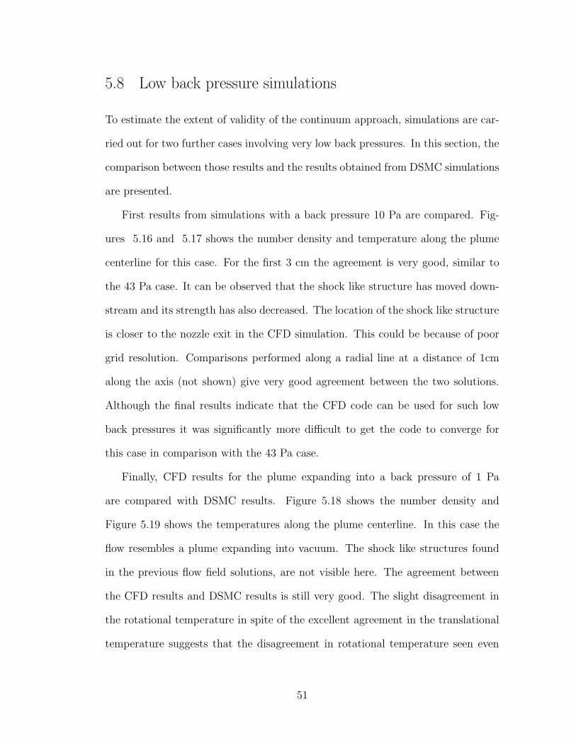
5.8 Low back pressure simulations

To estimate the extent of validity of the continuum approach, simulations are car-

ried out for two further cases involving very low back pressures. In this section, the

comparison between those results and the results obtained from DSMC simulations

are presented.

First results from simulations with a back pressure 10 Pa are compared. Fig-

ures 5.16 and 5.17 shows the number density and temperature along the plume

centerline for this case. For the first 3 cm the agreement is very good, similar to

the 43 Pa case. It can be observed that the shock like structure has moved down-

stream and its strength has also decreased. The location of the shock like structure

is closer to the nozzle exit in the CFD simulation. This could be because of poor

grid resolution. Comparisons performed along a radial line at a distance of 1cm

along the axis (not shown) give very good agreement between the two solutions.

Although the final results indicate that the CFD code can be used for such low

back pressures it was significantly more difficult to get the code to converge for

this case in comparison with the 43 Pa case.

Finally, CFD results for the plume expanding into a back pressure of 1 Pa

are compared with DSMC results. Figure 5.18 shows the number density and

Figure 5.19 shows the temperatures along the plume centerline. In this case the

flow resembles a plume expanding into vacuum. The shock like structures found

in the previous flow field solutions, are not visible here. The agreement between

the CFD results and DSMC results is still very good. The slight disagreement in

the rotational temperature in spite of the excellent agreement in the translational

temperature suggests that the disagreement in rotational temperature seen even

51

(XY) 1 Aug 1998


0

1

2

3

4

5

6

7

8

9

10N

umbe

rden

sity

(x10

22m

-3) DSMC

CFD

(XY) 1 Aug 1998

Figure 5.16. Comparison of number density along the plume centerline computedwith the CFD method and DSMC method at a back pressure of 10 Pa.

in the previous simulations is not due to rotational relaxation effects. The CFD

code seems to be able to predict the expansion region very well. Like the previous

case it was very difficult to obtain the converged solution.

52

(XY) 1 Aug 1998


0

25

50

75

100

125

150

175

200

Tem

pera

ture

(K)


(XY) 1 Aug 1998


53


0

1

2

3

4

5

6

Num

berd

ensi

ty(x

1022

m-3

)

DSMCCFD

Figure 5.18. Comparison of number densities along the plume centerline computedwith the CFD method and DSMC method at a back pressure of 1 Pa.

54

(XY) 1 Aug 1998


0

2

4

6

8

10

12

14

16

18

20T

rans

latio

nalT

empe

ratu

re(K

)

0

10

20

30

40

50

60

70

80

90

100

110

120

Rot

atio

nalT

empe

ratu

re(K

)


(XY) 1 Aug 1998


5.9 Conclusions

An upwind finite volume code for solving the Navier-Stokes equations on unstruc-

tured triangular grids was developed. A kinetics model for hydrogen consistent

with a previously developed DSMC model was implemented. It was successfully

applied to investigate low-density hydrogen plume flows. This completes the vali-

dation of the CFD code, which was the primary motivation for this study.

The two numerical results were found to be in good agreement with each other.

This validates the use of CFD codes as an efficient alternative to DSMC meth-

ods for performing such flow simulations. The comparison between the numerical

55

results and experimental measurements was found to be good in terms of overall

flow features. For a more detailed quantitative comparison higher resolution ex-

perimental measurements are required. The experimental measurements could not

be used to differentiate between the two computational methods. An assessment

of the validity of some of the equilibrium relations used for data reduction also

needs to be performed.

An important conclusion of this study is that these solutions exhibit a high

degree of grid dependence. This was found to be true of both the DSMC and CFD

computations. Thus care should be taken to ensure that the grid resolution is

fine enough to obtain accurate results. This emphasizes the importance of flexible

gridding techniques provided by the use of unstructured grids. For this system,

it is difficult to separate the results of the grid dependence from the physics of

the problem. An exhaustive grid independence study was not carried out since it

would not add to our understanding of the flow. Further refinement of the grid did

not improve the agreement with the experimental measurements.

From the above computations it can be concluded that, from the point of view

of application of CFD methods, these rarefied flows can be roughly divided into

three regimes. In the first regime, the back pressures are high enough to make

the application of CFD methods more efficient than particle based methods. In

the second regime, CFD methods can be applied but the difficulty in obtaining

a solution makes DSMC methods much more attractive. Presumably there is a

third region where the continuum approach breaks down and the CFD solutions if

obtainable would disagree with the DSMC results.

The main limitation of using this system for testing the combined approach

is that we could not clearly demonstrate the third region. Since DSMC simula-

56

tions could be performed for the nozzle itself, this system did not allow for a clear

demonstration of the need for the continuum approach. Thus a system with dif-

ferent flow conditions and more detailed experimental measurements is required to

clearly demonstrate the advantages of the combined methodology and the break-

down of the continuum approach. The following chapters present simulations of a

carbon dioxide expansion flow that does not have these limitations.

57

Chapter 6

Computation of the CO2 Nozzle flow

6.1 Introduction

This chapter and next two chapters present the details of a complete nozzle plume

simulation carried out by using the combined CFD DSMC methodology described

in chapter two. This chapter presents the simulations of the nozzle flow and com-

parisons with experimental measurements. The CFD code is applied to study

carbon dioxide expansion into hard vacuum. The results are compared with experi-

mental measurements made at Arnold Engineering Development Center (AEDC)[9].

An accurate assessment of plume impingement issues requires detailed under-

standing of the fluid dynamics and kinetics of the nozzle flow and plume flow. With

this in mind, several experimental and numerical studies were directed towards the

prediction and characterization of such flows. One such study was an experimental

test program instituted by the Air Force Rocket Propulsion Laboratory (AFRPL)

and performed in 1985 at the Arnold Engineering Development Center (AEDC).

The basic objective of that study was to define flow characteristics of pure-gas ex-

pansions into hard vacuum by obtaining a comprehensive database that could be

used to validate computational codes. The results from this study, previously clas-

sified, are now available in the open literature.[9] This represents the first attempt

to make detailed comparisons of these measurements with numerical computations.

58

Computer simulations are performed for the complete system from the inlet

of the nozzle to the outer plume regions. This chapter presents the results from

the CFD simulation of the nozzle flow and near plume region. These results are

compared with experimental measurements made by Bailey. Flow field results in

the plume region, an analysis of breakdown of continuum and results from the

simulation of the backflow region will be presented in the subsequent chapters.

6.2 Experimental Details

This section describes the experimental setup, the nozzle conditions and gives some

details of the configuration chosen for numerical investigation. The experiments

was described in detail by Bailey.[9]

6.2.1 Test facility

The experimental program was conducted in a 4 by 10 feet research vacuum cham-

ber (RVC) at the AEDC. The RVC is a stainless steel cylindrical vacuum chamber

with an internal diameter of approximately 3.5ft and an overall length of approxi-

mately 14ft. Vacuum conditions within the RVC are achieved through the use of

mechanical pumps, diffusion pumps and LN2 cryopumps. A number of basic inves-

tigations of various low-density phenomena were carried out at this test facility. A

wide range of flow diagnostic techniques was used to determine the characteristics

of the plume. The effects of nozzle area-ratio, lip geometry, chamber pressure, con-

densation, and cryopumping in the nozzle backflow region on the characteristics of

the plume were among the issues investigated.

59

6.2.2 Choice of nozzle and gas supply

The design of the test nozzles and the choice of the test gas took into account

the requirements of the test program, the operational characteristics of the RVC

and the results of earlier studies conducted in the RVC. CO2 expansions were

studied because they allowed the use of inexpensive LN2 cryopumping as opposed

to N2 expansions which would have necessitated the use of more expensive GHe

cryopumping. Earlier studies showed that acceptable background pressures (10−5

torr) could be achieved with nozzle flow rates of the order of 2 gm/sec. To simplify

nozzle design and fabrication, the study was limited to 15-degree half-angle conical

configurations with a fixed exit diameter of 4” and various throat diameters.

The evaluation of the mechanism affecting the flow of gas into the nozzle back-

flow region was an area of prime interest in the experimental study. It is generally

accepted that this gas flow derives from the expansion of the nozzle boundary

layer. Therefore, one of the requirements of the study was that the nozzle bound-

ary layer should be of sufficient thickness to permit spatially resolved flow field

measurements. The number density on the exit-plane centerline should be of the

order of 1015/cm3 in order to minimize the magnitude of the quenching corrections

required for electron beam fluorescence measurements. The stagnation tempera-

ture of the gas should be controlled such that condensation in the expanding flow

would occur downstream of the nozzle exit plane. With these constraints in mind,

nozzle stagnation conditions and throat diameter were chosen so as to produce an

acceptable flow at the nozzle exit plane.

Three nozzles with corresponding operating conditions were used for the ex-

perimental study. As a first attempt at detailed numerical analyses of these ex-

periments it was decided to choose one nozzle and study it in detail. Since the

60

focus of this investigation is more on the CFD aspect of these simulations, the

configuration with the maximum number of measurements in the continuum and

near continuum region is chosen.

This configuration involves a nozzle with a throat diameter of 0.6” and area-

ratio of 44.4. The stagnation temperature of the flow is 710K while the stagnation

pressure is 36.5 torr. The massflow rate through the nozzle was maintained at

1.77 ± 0.06 gm/sec. The numerical results are compared with pitot pressure mea-

surements along the plume centerline, flow angle measurements in the plume, and

electron beam fluorescence measurements of number density and rotational tem-

perature along the radial direction at a few axial stations. The objective of these

comparisons is to assess the validity of the numerical data and the accuracy of the

measured data.

6.3 CFD Computations

Similar to the previous study, a few modifications have to be made to the code to

perform simulations of carbon dioxide expansions. This section presents the details

of the kinetics model and the details of the boundary conditions that are specific

to this application.

6.3.1 Kinetics model for CO2

Carbon dioxide is linear tri-atomic molecule. It has three translational degrees of

freedom, and two rotational degrees of freedom. The characteristic temperatures

for the first three vibrational modes of carbon dioxide are 960K, 1290K and 3384K.

The 960K mode is degenerate with a degeneracy of two. Since the stagnation tem-

61

perature of the flow is 710K the last mode can be neglected without any significant

errors. The thermo-chemical processes modeled are translational-rotational relax-

ation and vibrational-translational relaxation. The vibrational relaxation rates are

obtained from Boyd[12]. All vibrational modes are assumed to be in equilibrium

with each other and to have the same relaxation rates. This assumption is made

due to the lack of information about separate modes. The rotational relaxation

rates are obtained from a previous study by Boyd[12]. The implementation of these

relaxation effects is similar to the one described in previous chapter.

For solutions of the Navier Stokes equations, viscosity has to be prescribed as a

function of the flow properties such as pressure or temperature. The viscosity model

used has a temperature coefficient of 0.67 and gives an excellent fit to measured

data.[12] This model has been used before for numerical studies of CO2 flows using

the DSMC method[12].

6.3.2 Boundary conditions

The simulation domain starts at the inlet to the nozzle and goes into the far-plume

region. There are four types of boundaries, the inlet to the nozzle, the nozzle wall,

the axis centerline and the outflow. Boundary conditions are implemented using

fictitious cells outside the boundaries. At the inlet plane the flow is sub-sonic. For

a CFD simulation, this allows us to specify two properties at the inflow boundary

while a third has to be extrapolated from inside the domain. From the experimental

measurements of the nozzle flow, mass-flow rate and stagnation temperature are

known and hence they are specified at the nozzle inlet. The velocity is extrapolated

from inside the domain. The axis centerline is implemented as a line of symmetry.

The outflow boundary condition depends on the Mach number of the flow

62

normal to the domain exit plane. If the flow is supersonic all the flow properties

are extrapolated from inside the flow domain. If the flow is subsonic the pressure

at the exit is assumed to correspond to the background pressure of the flow and

all other flow properties are extrapolated or calculated. Since the experiments

conducted were of the flow expanding into vacuum, the backgound pressure is very

low. For the simulations, the background pressure is set to a low value of 0.01 Pa.

The actual value of the pressure does not affect the flow. The domain is made

large enough so as to minimize the effects of the exit boundary conditions in the

regions of interest.

The nozzle wall is simulated using an isothermal wall boundary condition. The

CFD code requires the wall temperature as an input parameter. Since the stag-

nation temperature of the flow is 710K and the room temperature is 300K, it is

reasonable to expect the wall temperature to be bounded by these values. The

wall temperature may not be uniform and could vary from the nozzle throat to

the nozzle lip. For the simulations described in this chapter, the wall tempera-

ture is assumed to be uniform. Two simulations are performed, one with a wall

temperature at 300K and another with the wall temperature at 500K.

Calculating the boundary layer thickness provides a simple estimate of the effect

of the wall temperature. The boundary layer thickness on a flat plate is inversely

proportional to square root of the Reynolds’ number and therefore to the square

root of viscosity. This simple estimate predicts that the boundary layer for a wall

temperature of 500K would be about 25% thicker than the boundary layer for a

wall temperature of 300K. The CFD results can thus be expected to be sensitive

to the wall temperature.

63

0 0.1 0.2Axial Direction ( m )

-0.05

0

0.05

0.1

0.15

0.2

Rad

ialD

irect

ion

(m)

Grid used for CFD simulations

nozzle wall

nozzle exit plane

( €40,000 triangles )

nozzle throat

Lip region (refinement)

Figure 6.1. Grid used for the CFD computations

6.3.3 Grid resolution and other numerical issues

The domain starts at the inlet plane of the nozzle and extends about ten nozzle

radii from the nozzle exit-plane in the axial direction and about one nozzle radius

from the nozzle lip in the radial direction. The backflow region is not included as

the flow is expected to be highly non-continuum in that region. Figure 6.1 shows

a sample grid used for the simulations. The grid is clustered near the wall, the

nozzle throat, and the nozzle lip to adequately capture the flow. A grid independent

solution is obtained by repeating the simulations on finer grids until grid resolution

is sufficient. The coarse grid has around 10,000 cells while the final grid has about

40,000 cells. Only results from the final grid are presented in this chapter.

64

6.4 Comparison of CFD Results with Experimental Mea-

surements

This section presents the comparison of the results obtained from the CFD com-

putations with experimental measurements.

6.4.1 Pitot pressure

Measurements of centerline pitot pressure as a function of axial distance were made

using probes having diameters of 0.05”, 0.125” and 0.25”. The measurements

indicated that the pitot pressure was independent of probe size. The details of the

measurements are presented in Bailey’s report[9]. Pitot pressure is not directly

predicted by the simulations. It can however be calculated using the pressure,

temperature, and Mach number values predicted by the simulation along with

normal shock relations and γ, the ratio of specific heats. This last quantity is

calculated using information about the translational, rotational and vibrational

temperatures.

Figure 6.2 shows the comparison between the values calculated using the CFD

results and the measurements. The figure shows that the CFD results are sensitive

to the wall temperature. However, the two CFD results bound the experimental

results, thereby suggesting that a more accurate modeling of the wall boundary

conditions might result in better agreement between experimental and numerical

results. The 500K case shows better agreement with the experimental measure-

ments and is used for all other comparisons presented in this chapter.

In the experimental report, the measured values of pitot pressure, stagnation

temperature and stagnation pressure are used along with isentropic relations with

65

-0.1 0 0.1 0.2Axial Distance ( m )

0

100

200

300

400

500

600

700

800

900

1000

Pito

tPre

ssur

e(P

a)

Twall = 300Twall = 500Exp.

Nozzle Exit Plane

Figure 6.2. Comparison of centerline pitot pressure measurements with of datacalculated from the simulations

66

0 0.1 0.2 0.3 0.4 0.5Axial Distance ( m )

0

100

200

300

400

500

600

700

Tem

pera

ture

(K) Ttrans

TrotTvib

Figure 6.3. Centerline temperatures predicted by the simulation

67

the assumption that γ = 1.4 to derive the flow properties along the axis.[9] Since

the CFD simulations include detailed thermo-chemical modeling, the accuracy of

these assumptions can be assessed. Calculation of γ from the translational, ro-

tational and vibrational temperature data shows that it is close to 1.2 instead of

1.4 assumed for data reduction. Figure 6.3 shows profiles of different tempera-

tures along the axis centerline. The rotational and the translational modes are in

equilibrium throughout while the vibrational temperatures are almost frozen after

the nozzle throat. It should be noted that the vibrational temperature in these

non-equilibrium flows is simply an index of the energy contained in the vibrational

mode. Also the different modes of vibrational energy are not modeled separately,

thereby giving a single vibrational temperature. These finite rate processes are

irreversible and increase the entropy of the flow thereby violating the isentropic

assumption.

6.4.2 Flow angle

Flow angle was obtained by measuring the variation of the pitot pressure with

probe angle to the incident flow. The angle at which the maximum of pitot pressure

occurred was assumed to be the angle of the flow velocity vector at that position

in the nozzle plume.

One of the important conclusions of the experimental report is the re-affirmation

of some observations made by Bird[13] based on DSMC computations. Bird had

seen that in the boundary layer flow upstream of the nozzle lip, the local flow

angle is greater than the local angle of the nozzle wall i. e. the flow is directed

towards the nozzle wall rather than parallel to it. The experiments indicated that

flow angles of up to 30 degrees are possible in the exit plane, indicating local flow

68

0 0.25 0.5 0.75 1Normalized Radial Distance

0

5

10

15

20

25

30

35

40

Flo

wA

ngle

(deg

rees

)

Nozzle Half-Angle (local angle of the nozzle wall)

Figure 6.4. Flow angle across the nozzle exit plane

69

-0.5 0 0.5 1 1.5 2 2.5Normalized Axial Distance

0

0.5

1

1.5

2

2.5N

orm

aliz

edR

adia

lDis

tanc

e

0 1 20

0.25

0.5

0.75

1

1.25

1.5

1.75

2

2.25

2.5

5

7.510

15

20

30405060

nozzle wall

Figure 6.5. Comparison of contours of flow angles

angles with respect to the wall of 15 degrees, which is of the magnitude observed

in Bird’s studies. Figure 6.4 shows the flow angles predicted by the simulations at

the nozzle exit plane. The flow angles near the wall are close to 40 degrees. This

provides additional numerical evidence of this phenomenon. Thus, the Navier-

Stokes code used for this study is able to overcome the limitations of the boundary

layer codes mentioned in the experimental study which do not account for this

effect.

The flow angle data from the experimental measurements were presented as

contours of constant flow angle. To accomplish this, best-fit lines (by eye) were

drawn through the experimental data. To make comparisons with numerical data,

70

0 0.5 1 1.5 2 2.5 3Normalized Radial Distance

0

10

20

30

40

50

60

70

80

90

100F

low

Ang

le(d

egre

es)

Figure 6.6. Comparison of radial profiles of flow angles

the contour plots presented in Bailey’s report were digitized and plotted along with

flow angle contours obtained from the simulations. Figure 6.5 shows a comparison

between the flow angle measurements and numerical predictions. The location and

frequency of the symbols is an artifact of the digitization and do not have any

relevance to the experimental measurements. Taking into account the numerous

inaccuracies introduced, it can be concluded that the overall agreement is reason-

able. In the central-core region of the flow there is excellent agreement between

the measured values and the numerical predictions. As we go away from the nozzle

centerline, the CFD flow seems to show a larger deflection from the centerline than

that inferred from the experimental measurements.

71

Figure 6.6 presents a comparison of flow angle profiles along the radial direction

at four axial stations. The agreement deteriorates as we go away from the axis.

Bailey’s report suggests that flow angle measurements in regions of high shear

might be susceptible to probe flow interaction effects. Near the nozzle lip, the

probe bow shock may interact with the nozzle lip and lead to inaccuracies in the

measurements. As we go away from the centerline the plume flow becomes highly

rarefied and non-equilibrium effects become important. Under these conditions,

the underlying assumptions of the CFD code may not be valid leading to poor

results.

6.4.3 Number density and Temperature

Number density measurements, obtained using the electron beam fluorescence tech-

nique, were derived from measurements of the light intensity within a given spectral

interval of a vibrational-rotational band of a molecular species generated as a result

of the interaction of a narrow collimated beam of electrons with the gas species.

Figure 6.7 shows comparisons between axial profiles of number density. In order

to obtain accurate measurements of absolute number density using this technique,

it is necessary to calibrate the system in a gas of known number density. For

the experimental program, estimates of number density on the nozzle centerline

were derived from the measured value of pitot pressure, stagnation pressure, the

assumption of isentropic flow and a γ of 1.4. The electron beam calibration fac-

tor was selected on the basis of this calculated value of number density close to

the nozzle exit plane. This calibration method might have introduced additional

errors. Also the computed results are sensitive to the wall boundary conditions.

Keeping these two factors in mind, the overall agreement between the computed

72

-0.05 0 0.05 0.1 0.15Axial Distance ( m )

0

1

2

3

4

5

6

Num

berD

ensi

ty(x

1022

/m3

)

CFDExp.

Figure 6.7. Centerline number density from numerical calculations and experiments

73


1019

1020

1021

1022

Num

berD

ensi

ty(/

m-3

)

CFDExp.

Figure 6.8. Number density profiles along the radial direction at a distance of 0.27”from the nozzle exit plane

and measured values is satisfactory.

Figure 6.8 shows comparison between radial profiles of number density an axial

station 0.27” from the nozzle exit plane. The values reported by Bailey[9] are dig-

itized and plotted. The locations of the symbols are an artifact of the digitization

and do not have any significance to the experiments. There is good agreement be-

tween CFD results and experimental measurements in the core-flow region though

the CFD results are slightly higher. The agreement between the measured and

computed values deteriorates after a distance of about 1.3 nozzle radii from the

centerline. After that, the CFD number density drops at a much slower rate while

the experimental measurements show a continued rapid decrease in number den-

74

0 1 2 3 4Normalized Radial Distance

1018

1019

1020

1021

1022

Num

berD

ensi

ty(/

m-3

)

CFDExp.


sity. The CFD results may not be accurate in these regions because of the very

low number densities involved. The DSMC results and the breakdown parameter

calculations presented in the later sections support this conclusion.

Figure 6.9 shows comparison between radial profiles of number density at a

second axial station, 1.27” from the nozzle exit plane. Here the agreement is good

throughout the region of comparison. The experimental profiles show an off axis

peak in the number density. The maximum number density occurs at the edge

of the high-density core region rather than on the centerline. Bailey[9] concluded

that this was not an artifact of the measurement technique based on experimental

data obtained from previous studies. These off-axis peaks can be observed in the

75


50

75

100

125

150

175

200

225

250

275

300

325

350T

empe

ratu

re(K

)

Exp-Station1Exp-Station2CFD-Station1CFD-Station2

Figure 6.10. Rotational temperature profiles along the radial direction at the twoaxial stations

simulation results also, thereby confirming the assumption that they are indicative

of changes in the flow field properties in the core-flow region. These off-axis peaks

are not as prominent in the simulation results as they are in the experimental

measurements.

Rotational temperature was determined by the measurement of the spectral line

intensity distribution within a vibrational-rotational band of a molecular species

generated as a result of the interaction of a narrow collimated beam of electrons

with the gas species. These measurements used isentropic prediction of the exit-

plane rotational temperature for calibration, which may have affected the accuracy

of these measurements. The nozzle centerline value of 108K seen in the experimen-

76

tal results is the same as the isentropic prediction for temperature at this station

with a γ of 1.4.Figure 6.10 shows the rotational temperature comparisons at the

two axial stations. The CFD predictions of the temperatures are much higher

than the experimental measurements. The experimental measurements and the

CFD results show similar behavior although the experimental data show a much

steeper drop in the expansion region. The CFD results predict a peak temperature

of about 325K while the experiments show a peak of about 160K.

6.5 Conclusions

This chapter presents the comparison between CFD results and experimental mea-

surements obtained at the AEDC. The computational results were found to be

sensitive to the wall temperature. Experimental measurements of pitot pressure

along the centerline were compared with calculations based on the CFD simula-

tions. The computed values were close enough to experimental measurements to

suggest that the physics of the flow was captured accurately. A more detailed

modeling of the wall boundary condition might give better numerical agreement

with the measured results.

Detailed relaxation modeling of the different energy modes of CO2 indicated

that the vibrational mode was frozen in the diverging portion of the nozzle and

in the plume. The CFD simulations also predicted regions of rotational non-

equilibrium inside the plume. The central core region of the flow was non-isentropic

and had a ratio of specific heats close to 1.2. This invalidates the isentropic flow

assumption and the value of 1.4 used for calibrating some of the experimental

measurements.

77

The computations re-confirmed earlier findings about the behavior of the flow

near the nozzle lip. Flow angle measurements were compared with the computed

values and found to agree in the central-core region of the flow. The CFD predic-

tions of radial profiles of number density showed good agreement within regions of

validity of the continuum approach.

This completes the presentation of the results for the nozzle and near plume

region. Results in the plume and an analysis of breakdown of continuum will be

presented in the next chapter.

78

Chapter 7

Breakdown of continuum

After validating the CFD code and performing the nozzle flow simulations, the

next step in the development of the combined methodology is the investigation of

breakdown of the continuum approach. This chapter presents parameters that can

be used to predict breakdown of continuum. The results from CFD computations

are compared with results from DSMC computations. The numerical results are

then compared with experimental results to assess the validity of the continuum

assumption. The DSMC simulations are analyzed in detail to explain the failure

of the continuum approach

7.1 Introduction

The CFD method has physical and numerical limitations that prevent it from

being used for very rarefied flows. Since the outer plume and back-flow regions

involve very low densities, the DSMC method is used for performing simulations

in these regions. For the most efficient utilization of the two methods, a method

for accurately determining the validity of the continuum approach is required. In

the combined methodology, the CFD results are analyzed and a parameter based

on the flow properties is calculated and used to assess the validity of the CFD

simulation.

79

This chapter looks at a few possible parameters. A new parameter is presented

which is used to split the domain into a CFD region and a DSMC region. DSMC

simulations are then performed. The DSMC simulations are initialized with the

results from CFD simulation. The results obtained from the DSMC simulations

are compared with the CFD results. The numerical results are also compared with

experimental measurements.

One of the objectives of this study is to investigate a flow regime where the CFD

approach breaks down and the DSMC approach gives accurate results. Compar-

isons with experimental measurements are performed with the objective of finding

a region where the experimental measurements agree with the DSMC results and

disagree with the CFD results. The DSMC results in this region are then analyzed

in detail to understand why the CFD method fails to make accurate prediction of

the flow properties.

7.2 Prediction of breakdown

The breakdown of the Navier-Stokes equations under conditions of low-density,

hypersonic flow has been investigated before by Boyd et al[14] and for expanding

flows by Bird[13]. Both papers present parameters which can be used for prediction

of breakdown of the continuum approach.

7.2.1 Parameters used in previous studies

The gradients of the macroscopic flow properties in an isentropic flow depend

only on the size of the flow. However, these changes in the macroscopic flow

properties can occur only through intermolecular collisions and, as the density

80

falls, the collision rate becomes too low for the maintenance of these gradients.

Bird studied the occurrence of this type of breakdown in gaseous expansions and

found that the breakdown correlates with a parameter

P = −1

ν(D(ln ρ)

Dt), (7.1)

where ν is the collision frequency and ρ is the density. DDt

refers to the substantial

derivative. For a steady flow, this equation can be written as

P = −π

1

2

2sλ

ρ(dρ

dx). (7.2)

Here s is the speed ration, λ the local mean free path and the gradient is evaluated

in the stream-wise direction. The initial breakdown in both steady and unsteady

expansions was found to correlate with a value of P of approximately 0.04, thereby

giving an empirical criterion for breakdown.

The evaluation of the gradient in the stream-wise direction introduces the veloc-

ity components into the evaluation of the breakdown parameter leading to possible

problems at stagnation points and low velocity flows. Boyd studied a variety of

breakdown parameters and concluded that a Knudsen number based on the local

density-gradient length scale is best suited for most applications. Studies indicate

that the continuum approach fails when this breakdown parameter approaches

0.05.[14]

There are two problems with using these parameters for a combined CFD-

DSMC approach. The cut-off value of these parameters is empirical and might

vary with geometry and flow conditions. These parameters are based on density

gradients and do not consider gradients of other macroscopic properties. When

using a combined approach, a parameter that shows a clear distinction between

regions where the CFD solution is valid and regions where it is not valid would be

81

ideal. Since the breakdown of the CFD approach is related to viscosity and heat

transfer, it should take both these transport phenomena into account.

7.2.2 Chapman-Enskog Approach

It is possible to approach the prediction of breakdown from a kinetic theory view-

point. The Navier-Stokes equations can be derived from the Chapman-Enskog

solution to the Boltzmann equation. The Chapman-Enskog solution results from

an expansion of the velocity distribution function for small departures from the

Maxwellian distribution function present at equilibrium. The Chapman-Enskog

distribution function can be written as

f( ~C) = f0( ~C)Γ( ~C), (7.3)

where f0( ~C) is the Maxwell-Boltzmann velocity distribution function, where ~C =

C/√

2kT/m is the velocity normalized with the thermal velocity, k is the Boltz-

mann constant, T is the temperature and m is the particle’s mass.

Γ( ~C) = 1 + (qxCx + qyCy + qzCz)(25C2 − 1)

−2(τx,yCxCy + τx,zCxCz + τy,xCyCz)

−τx,x(C2x − C2

z ) − τy,y(C2y − C2

z ) (7.4)

and

qi = −κ

p(2m

kt)1/2 ∂T

∂xi

(7.5)

τi,j = −µ

p(∂vi

∂xj

+∂vj

∂xi

−2

3

∂vk

∂xk

δi,j) (7.6)

82

where τi,j and qi are the dimensionless heat flux and the stress tensor[16]. The

viscosity and thermal conductivity are µ and κ, respectively. vk is the fluid velocity

and T is the temperature. Cx, Cy and Cz are the components of ~C and C is the

speed.

This derivation assumes the perturbation to the Maxwellian to be small com-

pared to 1. Thus the magnitude of this perturbation gives an indication of the

validity of the Navier-Stokes equations. This approach takes into account both

transport phenomena. Momentum transfer is accounted for through the shear

stress terms in the expression and heat transfer through the thermal stress terms.

This expression is evaluated using the mean velocity, the shear stress and heat

fluxes obtained from a Navier-Stokes simulation and can be used to assess the

validity of the simulation.

The other advantage of using this parameter is evident when we examine the

radial profiles of the breakdown parameter. Figure 7.1 shows the breakdown pa-

rameters plotted along the radial direction at an axial station 0.27” from the nozzle

exit. The Chapman-Enskog factor gives a clear limit for the size of the CFD do-

main. It can be seen that after about 0.9 nozzle radii this factor falls rapidly. This

can be also verified in Fig. 7.2 which shows the three parameters plotted at an-

other axial station, 1.27” from the nozzle exit. In this case, as expected breakdown

is predicted at a greater distance from the axis. The comparisons between CFD

results and experimental measurements of number densities at these stations are

presented in the earlier section, Figs. 6.8 and 6.9. The CFD results agree with

experimental measurements for about .25 times the nozzle radius. Thus this pa-

rameter does not exactly predict where the CFD results are not accurate but gives

us a good indication of the appropriateness of using the CFD code without any

83

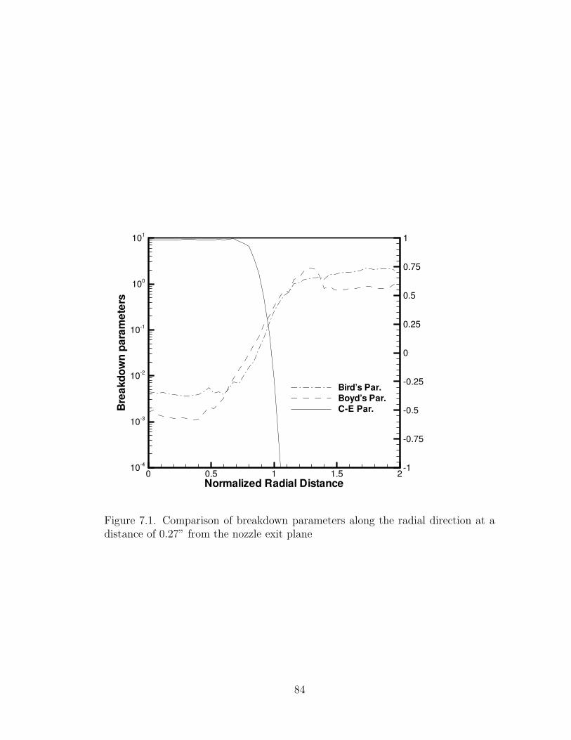
0 0.5 1 1.5 2Normalized Radial Distance

10-4

10-3

10-2

10-1

100

101

Bre

akdo

wn

para

met

ers

-1

-0.75

-0.5

-0.25

0

0.25

0.5

0.75

1

Bird’s Par.Boyd’s Par.C-E Par.

Figure 7.1. Comparison of breakdown parameters along the radial direction at adistance of 0.27” from the nozzle exit plane

84

0 0.5 1 1.5 2Normalized Radial Distance

10-3

10-2

10-1

100

Bre

akdo

wn

para

met

ers

-1

-0.75

-0.5

-0.25

0

0.25

0.5

0.75

1

Bird’s Par.Boyd’s Par.C-E Par.

Figure 7.2. Comparison of breakdown parameters along the radial direction at adistance of 1.27” from the nozzle exit plane

85

reference to any empirical factors. Since the breakdown criterion is not totally

empirical, this method could be applied to the study of other flows also.

7.3 DSMC simulations of the outer-plume region

The DSMC code used is described in chapter four. For this study the code is

used with unstructured triangular grids. A sub-cell method[18] is used to reduce

the computational cost. The results from the CFD simulations are used as inflow

boundary conditions for the DSMC code. Maxwellian distributions of velocities are

assumed at the inflow. Since the CFD simulations showed very little change in the

vibrational temperature in the plume, the vibrational mode is assumed to be frozen

and is not included in the DSMC simulations. Thus the gas is assumed to have

3 translational modes and 2 rotational modes of freedom. The implementation of

rotational relaxation is based on an earlier work by Boyd et al.[12].

The simulations are performed on an IBM SP2. There are about 1.2 million

particles in the simulation. The grid used has about 10,000 cells resolved to the

level of about 5 times the mean free path. Sub-cells are of uniform size and resolved

to the level of the smallest mean free path. Care was taken to ensure that at least

a few particles per sub-cell are present. Figure 7.3 shows the grid used for the

DSMC simulations.

86

0.1 0.2 0.3 0.4 0.5Axial Direction ( m )

-0.05

0

0.05

0.1

0.15

0.2

0.25

0.3

Rad

ialD

irect

ion

(m)

Grid used for DSMC simulations

nozzle wall

nozzle exit plane

( €10,000 triangles )

Figure 7.3. Grid used for the DSMC computations

87


1018

1019

1020

1021

1022

Num

berD

ensi

ty(

/m-3

)

CFDDSMCExp.

DSMC domain begins


88

7.4 Comparison of the DSMC results with CFD results and

experiments

The results obtained from the DSMC simulation are compared with results ob-

tained from the CFD computations. To assess the accuracy of these numerical

results, they are compared with experimental measurements. Figure 7.4 shows

the number density profiles at 0.27” from the nozzle exit plane along the radial

direction. The solid line and the dotted line represent the values obtained from

DSMC and CFD simulations respectively. The symbols represent values obtained

from experimental measurements. The DSMC domain begins about half a nozzle

radius from the axis centerline. Up to about 1.2 times the nozzle radius there is

good agreement between all three values. The CFD results then diverge away from

the other two results. There is good agreement between DSMC predictions and

experimental measurements of number density throughout the region of measure-

ment. Since both the CFD and the DSMC methods use similar kinetics models,

the agreement between DSMC results and experimental measurements seems to

indicate that the continuum approach is not valid in these regions. This is further

supported by the calculated breakdown parameter values shown in Fig. 7.1. It

can be seen that all three breakdown parameters predict breakdown of the Navier-

Stokes equations before the CFD number density starts differing from the other

two.

Figure 7.5 shows a similar plot with the number density profiles at 1.27”

from the nozzle exit plane along the radial direction. There is very good agree-

ment between numerical results and experimental measurements of number density

throughout the region of measurement. The behavior shown by the CFD results

89

[c]

0 1 2 3 4Normalized Radial Distance

1018

1019

1020

1021

1022

Num

berD

ensi

ty(/

m-3

)

CFDDSMCExp.


90

(XY) 17 Jun 1999

0 0.025 0.05 0.075 0.1Y

50

100

150

200

250

300t

0 1 2 3Normalized Radial Distance

0

50

100

150

200

250T

empe

ratu

re(K

)

DSMC-TTaTnCFD-T

Figure 7.6. Translational temperature profiles along the radial direction at atdistance of 0.27” from the nozzle exit plane

in the previous station may be starting to appear at the edge of the CFD domain.

7.5 Analysis of breakdown

This section presents the analysis of DSMC results for a better understanding of the

breakdown of Navier-Stokes equations. Figure 7.6 shows radial profiles of temper-

atures at 0.27” from the nozzle exit plane. The solid line is the DSMC prediction

of translational temperature. The two dashed lines show component-wise temper-

ature profiles. The axial temperature falls rapidly from its peak close to the nozzle

lip and reaches a very small value about 2 nozzle radii from the axis centerline.

91

The normal temperature freezes at 150K at a distance of 1.15 nozzle radii from

the axis centerline. The number densities in these regions are very low and there

are not enough collisions to maintain the drop in temperature predicted from ge-

ometric considerations. The Navier-Stokes equations are based on the assumption

of translational equilibrium and involve a single translational temperature. The

dotted line shows the translational temperature predicted by the CFD simulations.

Since the rate of decrease of temperature is imposed on the CFD solution from ge-

ometric considerations, the CFD translational temperature continues to drop. As

the normal temperature freezes, the DSMC translational temperature flattens out.

So after about 1.2 nozzle radii from the centerline the CFD predictions of temper-

ature fall below the DSMC predictions. Since pressure is determined mainly from

momentum considerations, the continued drop in temperature is compensated by

a flattening number density profile. Thus the CFD predictions of number density

are higher than the experimentally measured values and the DSMC predictions.

Figure 7.7 shows the number density results presented earlier superimposed on

a plot of the ratio of normal to axial temperature. This ratio can be considered as

an index of translational non-equilibrium. At about 1.2 nozzle radii from the axis

centerline this ratio falls rapidly indicating the onset of freezing. It can be seen

that in regions where freezing has occurred, the CFD results are not accurate.

Figure 7.8 shows the rotational temperature profiles at 0.27” from the nozzle

exit plane along the radial direction. The solid line and the dotted line represent

the values obtained from DSMC and CFD simulations respectively. The symbols

represent values obtained from experimental measurements. There is reasonable

agreement between the CFD and DSMC results while the experimental measure-

ments are much lower. Figure 7.9 shows a similar plot with the temperature profiles

92


1018

1019

1020

1021

1022

Num

berD

ensi

ty(/

m-3

)

0

0.1

0.2

0.3

0.4

0.5

0.6

0.7

0.8

0.9

1

1.1

Rat

ioof

Ta

toT

r

CFDDSMCExp.Ta / Tr (DSMC)

Figure 7.7. Number density profiles along the radial direction at a distance of 0.27”from the nozzle exit plane with an index of translational-equilibrium

93


50

75

100

125

150

175

200

225

250

275

300

325

350

Tem

pera

ture

(K)

CFDDSMCExp

Figure 7.8. Temperature profiles along the radial direction at a distance of 0.27”from the nozzle exit plane

94


0

50

100

150

200

250

Tem

pera

ture

(K)

CFDDSMCExp

Figure 7.9. Temperature profiles along the radial direction at a distance of 1.27”from the nozzle exit plane

95

at 1.27” from the nozzle exit plane along the radial direction. The DSMC results

and the CFD results show some difference. As shown in the previous section these

regions involve flow regimes with translational non-equilibrium effects, which are

not considered by the Navier-Stokes solver. The interface between the CFD region

and the DSMC region is located where the temperature starts to increase. When

the DSMC code is initialized this gradient information is not passed on to it and

is therefore lost. These factors may account for the discrepancy between the two

numerical results.

7.6 Conclusions

A breakdown parameter that can be used to split the computational domain into

two regions, one to be solved using CFD methods and the other to be solved using

DSMC methods, was presented. This parameter was used to split the domain by

predicting the breakdown of the Navier-Stokes equations. DSMC simulations, of

regions where CFD methods are not accurate, were performed. The DSMC predic-

tions of radial number density profiles were then compared with the experimental

measurements and found to be in good agreement, even in regions where the CFD







Thus a methodology for performing simulations of a complete nozzle-plume

96

system was described. It involves a CFD simulation of the nozzle and near plume

region, a breakdown parameter for splitting the domain, and a DSMC simulation

of the outer plume regions where CFD is not valid. This approach is successfully

applied to the study of CO2 expansion into hard vacuum. The next step is to

extend the simulation domain and perform simulations of the back flow region.

97

Chapter 8

Computation of back flow

This chapter describes the computation of the backflow region of the same carbon

dioxide flow considered in chapter seven. The back flow region has very low number

densities and is most accurately modeled using a DSMC computation. The DSMC

computation is initialized using results from a CFD computation of the nozzle flow.

8.1 Introduction

Chemical rockets are used extensively for attitude control and other low thrust

operations on trans-atmospheric vehicles and spacecraft. The interaction of the

plumes from these rockets with the vehicle surface is a major source of concern

for these applications. Plume impingement on the vehicle surface might lead to

contamination of sensitive surfaces, thrust losses, disturbance torques and thermal

loading. An accurate assessment of these issues requires detailed understanding of

the fluid flow in the back-flow region.

This chapter presents the results of investigations on different methods for per-

forming back-flow simulations. The computational results are compared with ex-

perimental measurements. Bailey’s[9] study presents experimental measurements

made in the back-flow region of the nozzle. The objective of our study is to in-

vestigate different methods for performing back-flow simulations and assess them

98

using these experimental measurements.

Two experimental measurements are performed in the backflow region. Carbon

dioxide number density measurements were accomplished using the electron beam

fluorescence technique. Mass flux measurements were made in the back-flow region

using a Quartz crystal microbalance. The computational results are compared with

these experimental results.

First, a CFD computation of the nozzle and near plume region is performed.

The Chapman-Enskog parameter described in the previous chapter is then used

to predict breakdown. The DSMC domain starts where the Chapman-Enskog

parameter has a value of 0.95. The grid used is show in figure 8.1. Bailey’s report

mentions that the results are sensitive to lip geometry. Care has therefore been

taken to model the lip region in detail. The grid used has about 10,000 cells

resolved to the level of about 5 times the mean free path.

A description of the DSMC code is presented in chapter four. A sub-cell

method[18] is used to reduce the computational cost. The simulations are per-

formed on an IBM SP2. There are approximately 1.2 million particles in the

simulation. Sub-cells are of uniform size and resolved to the level of the smallest

mean free path. Care is taken to ensure that at least a few particles per sub-cell

are present.

The results from the CFD simulations are used as inflow boundary conditions

for the DSMC code. Two methods of passing the information from the CFD

simulations to the DSMC simulations are investigated. Since the CFD simulations

show very little change in the vibrational temperature in the plume, the vibrational

mode is assumed to be frozen and are not included in the DSMC simulations. Thus

the gas is assumed to have 3 translational modes and 2 rotational modes of freedom.

99

0.1 0.2 0.3 0.4 0.5X

0

0.05

0.1

0.15

0.2

0.25

0.3

0.35

Y

Figure 8.1. Grid used for the DSMC simulations

100

The implementation of rotational relaxation is based on an earlier work by Boyd

et al.[12].

8.2 DSMC computation with Maxwellian boundary condi-

tion

The results from the CFD simulations are used as inflow boundary conditions

for the DSMC code. The fluid properties need to be specified at the inlet of the

domain. The temperature, velocity and number density are obtained from the CFD

simulation and imposed as inflow boundary conditions in the DSMC simulation.

In addition to this, a velocity distribution also needs to be specified. The simplest

method is to assume a Maxwellian distribution of velocities at the inflow. This

is not strictly correct and the accuracy of this assumption and its effect on the

simulations are assessed in the next section.

8.2.1 Flow field Results

Initially simulations were performed with the flow assumed to expand into vacuum.

Figure 8.2 shows the number density contours obtained from these simulations. It

can be seen that in the back flow region the number density is of the order of

1 × 1018m−3. In Bailey’s report the back pressure is reported to be about and

2 × 10−5 torr. At temperatures of 300K this corresponds to a number density of

6.77× 1017m−3. This suggests that the back pressure could influence the flow field

in this region. Thus from this simulation it can be observed that the back pressure

needs to be simulated to obtain a closer simulation of the experimental set-up.

Figure 8.3 shows the number density contours obtained from simulations with a

101

0 0.1 0.2 0.3 0.4 0.5 0.6Axial Distance

0

0.05

0.1

0.15

0.2

0.25

0.3

0.35

0.4

0.45

0.5R

adia

lDis

tanc

e

1E+18 5E+18

1E+1

9

5E+191E+20

5E+20

1E+21

3E+21

5E+21

1E+223E+22

Figure 8.2. Number density profiles for simulations of CO2 expanding into vacuum

back pressure of 2 × 10−5 torr.

8.2.2 Comparison with experiments

Two experimental measurements are performed in the back flow region. Carbon

di-oxide number density measurements were accomplished using the electron beam

fluorescence technique. Radial profiles of number density were measured and a

smoothed spatial map of constant number density was derived. Figure 8.4 shows

the comparison of the number density measurements with the number density

obtained from the simulations. The agreement between the simulation results and

the measured values deteriorate as we go into the back-flow region. The simulations

102

0 0.1 0.2 0.3 0.4 0.5 0.6Axial Distance

0

0.05

0.1

0.15

0.2

0.25

0.3

0.35

0.4

0.45

0.5

Rad

ialD

ista

nce

5E+18 1E+19

5E+19

1E+20

1E+20

5E+20

1E+213E+21

Figure 8.3. Number density profiles for simulations with ambient number densityof 6.77e17 / m3

103

-0.05 0 0.05 0.1 0.150

0.05

0.1

0.15

0.2

0.25

2e18

5e18 1e192e19

5e19

1e20

4e21 3e21 2e21

1e21

-0.05 0 0.05 0.1 0.15Axial Distance (m)

0

0.05

0.1

0.15

0.2

0.25R

adia

lDis

tanc

e(m

)

2E+18 5E+18 1E+19

2E+19

5E+19

1E+20

2E+20

1E+21

2E+21

Number density contours ( background pressure = 2e-5 torr)

Figure 8.4. Comparison of measured and calculated data for the number densityin the back-flow region

have an ambient number density of 6.77×1017m−3, which corresponds to a pressure

of 2× 10−5 torr and a temperature of 300K. It is possible that the actual ambient

number density is higher than 6.77 × 1017m−3 and that would explain why the

computed results are lower than the experimental measurements.

Figure 8.5 shows the number density contours obtained from a simulation with

ambient number density set at 1 × 1018m−3. particles / m3. Figure 8.6 shows a

comparison of number density contours obtained from simulations with an ambient

number density of 1e18. This sensitivity study shows that the ambient number den-

sity has a strong influence on in the regions where experimental measurements are

made. Since the exact modeling of the back pressure distribution in the chamber

104

0 0.1 0.2 0.3 0.4 0.5 0.6Axial Distance

0

0.05

0.1

0.15

0.2

0.25

0.3

0.35

0.4

0.45

0.5

Rad

ialD

ista

nce

5E+18

1E+213E+21

1E+19

5E+20

1E+20

1E+19

5E+19

2E+1

8

Figure 8.5. Number density profiles for simulations with an ambient number den-sity of 1 × 1018m−3

105

0.1 0.2 0.3 0.4 0.5X

-0.2

-0.15

-0.1

-0.05

0

0.05

0.1

0.15

0.2

Y

1.25

E+1

8

2.5E+18

5E+1

81E+19

2E+194E+19

1E+20

5E+20

1E+21

5E+201E+21

1E+20

4E+19

2E+191E+19

5E+18

2.5E+18

1.25E+18

Ambient number density = 6.77e17

Ambient Number density : 1.00E18

Figure 8.6. Comparison of number density profiles for simulations with an ambientnumber density of 1×1018m−3 and and ambient number density of 6.77×1017m−3

106

-0.05 0 0.05 0.1 0.150

0.05

0.1

0.15

0.2

0.25

-0.05 0 0.05 0.1 0.15Axial Direction (m)

0

0.05

0.1

0.15

0.2

0.25R

adia

lDire

ctio

n(m

)

2E-0

9

5E-1

01E

-09

Massflux Measurements (kg/sec)

5e-101e-9

2e-9

Figure 8.7. Comparison of measured and calculated data for the mass flow rate inthe back-flow region

is very difficult, this suggests that further improvement in the agreement between

computed and measured values is difficult.

Mass flux measurements were made in the back-flow region using a Quartz crys-

tal microbalance. Figure 8.7 shows a comparison of the mass-flux measurements

and the values calculated from the experiments. Summaries of the experimental

measurements were presented as constant mass flux contours and compared with

numerical results. Since there are only three contours it is difficult to make details

comparisons but the results are consistent with the number density results.

107

8.3 DSMC computation with Chapman-Enskog boundary

condition

This section presents the results of the investigation of a more accurate method

of passing information from the CFD simulations to the DSMC simulation. The

results from this new method are compared with the old method and experimental

measurements.

8.3.1 Rationale

The boundary conditions for the DSMC simulations are set using the results from

the CFD simulation. The gas properties (number density, temperature and veloc-

ity) need to be specified at the domain inlet. A velocity distribution function also

needs to be specified at the inlet. Normally in DSMC simulations, thermodynamic

equilibrium is assumed at the boundary and the velocity distribution is set using

the Maxwell-Boltzmann distribution,

f0(C) =1

π3/2exp(−C2), (8.1)

where C = c / (2kT/m)1/2 is the normalized thermal velocity, c is the velocity,

k is the Boltzmann constant, T is the temperature and m is the particle mass. The

results in the preceding section were obtained using this method.

For non-equilibrium flows, the Chapman-Enskog distribution is a better approx-

imation. The Chapman-Enskog perturbation expansion of the Boltzmann equation

gives, to first order in Sonine polynomial expansion, the distribution

f(C) = f0(C)Γ(C), (8.2)

108

where

Γ(C) = 1 + (qxCx + qyCy + qzCz)(25C2 − 1)

−2(τx,yCxCy + τx,zCxCz + τy,xCyCz)

−τx,x(C2x − C2

z ) − τy,y(C2y − C2

z ) (8.3)

and

qi = −κ

P(2m

kt)1/2 ∂T

∂xi(8.4)

τi,j = −µ

P(∂vi

∂xj+

∂vj

∂xi−

2

3

∂vk

∂xk∂i,j) (8.5)

where τi,j and qi are the dimensionless heat flux and the stress tensor[16]. The

viscous and thermal conductivity are µ and κ, respectively.

8.3.2 Implementation

The Chapman-Enskog distribution is implemented using an acceptance rejection

technique described in Garcia[16]. An envelope function g(C) is defined such that

g(C) > f(C) for all C. Then a random point from the region beneath g(C) is

selected. All points in this region are equally likely to be selected. A simple way to

select this point is to use g(C) = A f0(C), where f0(C) is the Maxwell-Boltzmann

distribution. A velocity Ctry is drawn from f0(C) and is accepted if this point lies

beneath f(C). Otherwise a new point is drawn and the procedure is repeated. More

details about this procedure are described by Garcia[16].

At the interface between the two domains Γ(C) has a value of about 0.95.

Figure 8.8 shows the contours of the Chapman-Enskog parameter calculated using

109

[c]

0 0.1 0.2 0.3 0.4 0.5 0.6Axial Distance (m)

0

0.1

0.2

0.3

0.4

0.5

Rad

ialD

ista

nce

(m)

0.90.2 0.8Nozzle Wall

C-E parameter contours

Figure 8.8. Contours of Chapman-Enskog parameter calculated based on the CFDsolution

110

0.1 0.2 0.3 0.4 0.5X

-0.2

-0.15

-0.1

-0.05

0

0.05

0.1

0.15

0.2Y

1.5E+1

82E

+18

5E+18

5E+19

1E+20

5E+20

1E+214E+21

4E+21

CE Boundary Condition

Maxwell Boltmann Boundary Condition

Figure 8.9. Comparison of contours of number density

the mean velocity. As described in the previous chapter, a value of Γ(C) = 0.95 is

assumed to be a safe indication of the validity of Navier-Stokes equations.

8.3.3 Comparison of results

The objective of this section is to compare the two different methods of passing

information. Figure 8.9 shows a comparison of the number density contours ob-

tained from the two methods. The agreement between the two methods is fairly

good and there does not seem to be any appreciable difference between the two

results.

Figure 8.10 shows a more detailed comparison of the number density at a radial

111

0.05 0.1 0.15Y

1018

1019

1020

1021

1022

ρ

CE-dataMB-data

Number density profiles near the exit plane

Figure 8.10. Number density along a radial section at the exit plane

section along the exit plane of the nozzle. This comparison shows few differences

although the over all behavior is very similar. The results obtained from the

application of the Chapman-Enskog boundary condition are lower than the results

from the Maxwell-Boltzmann boundary conditions.

Figure 8.11 and figure 8.12 shows a comparison of these results with the ex-

perimental measurements. The comparisons are very similar to the comparisons

obtained from the Maxwell-Boltzmann results. It is difficult to assess the impor-

tance of using the Chapman-Enskog boundary conditions from these results. More

detailed measurements in the back-flow region is required to perform a more de-

tailed analysis of the two boundary conditions. In this study the results obtained

112

-0.05 0 0.05 0.1 0.15V1

0

0.05

0.1

0.15

0.2

0.25V

2

-0.05 0 0.05 0.1 0.15X

0

0.05

0.1

0.15

0.2

0.25Y

4E-0

91E-09

Figure 8.11. Comparison of measured and calculated data for the number densityin the back-flow region

from the two boundary conditions are similar.

8.4 Conclusions

The objective of this study was to investigate different methods of performing back

flow simulations. The combined CFD-DSMC method can be used to obtain results

in the back flow region. The back flow region was found to be very sensitive to the

ambient conditions and an accurate simulation of the back pressure is essential.

The simulation results show lower number densities than observed experimentally.

A more accurate assessment of these issues requires more measurements to compare

113

-0.05 0 0.05 0.1 0.15V1

0

0.05

0.1

0.15

0.2

0.25

V2

-0.05 0 0.05 0.1 0.15X

0

0.05

0.1

0.15

0.2

0.25

Y

Figure 8.12. Comparison of measured and calculated data for the mass flow ratein the back-flow region

114

the numerical results. Two methods for transferring information to the DSMC

simulation are compared. The two methods were found to give very similar results

and so Maxwell Boltzmann boundary conditions were found to be sufficient.

115

Chapter 9

Summary and conclusions

The objective of this dissertation was to develop a methodology for performing

simulations of a complete nozzle plume system. A combined CFD-DSMC approach

for performing these simulations was developed.

The combined approach involves four steps. First, a continuum simulation of

the nozzle plume system is performed. An unstructured Navier-Stokes solver for

performing these simulations was developed. The next step involves predicting

the breakdown of Navier-Stokes equations from the CFD simulations and dividing

the domain into a CFD region and a DSMC region. Various parameters that

could be used for this were investigated and a new parameter was proposed. The

third step involves transferring information from the CFD simulation to the DSMC

simulation. Different methods of transferring information were analyzed. The last

step involves performing DSMC simulations. DSMC simulations were performed

and the results were analyzed to understand more about the breakdown of the

Navier-Stokes equations.

The method was applied to the study of two nozzle systems for which experi-

mental results were available. The first system involved was a hydrogen thruster.

A kinetics model for hydrogen consistent with a previously developed DSMC model

was implemented. It was successfully applied to investigate the low-density hydro-

gen plume flows.

116

The comparison between the numerical results and experimental measurements

was found to be good in terms of overall flow features. For a more detailed quanti-

tative comparison higher resolution experimental measurements are required. The

experimental measurements could not be used to differentiate between the two

computational methods. An assessment of the validity of some of the equilibrium

relations used for data reduction also needs to be performed. An important conclu-

sion of this study is that these solutions exhibit a high degree of grid dependence.

This was found to be true of both the DSMC and CFD computations. Thus care

should be taken to ensure that the grid resolution is fine enough to obtain accurate

results. This emphasizes the importance of flexible gridding techniques provided

by the use of unstructured grids. For this system, it is difficult to separate the

results of the grid dependence from the physics of the problem. An exhaustive grid

independence study was not carried out since it would not add to our understand-

ing of the flow. Further refinement of the grid did not improve the agreement with

the experimental measurements.

The next system analyzed was the expansion of carbon di-oxide into vacuum.

The computational results were found to be sensitive to the wall boundary condi-

tion. Experimental measurements of pitot pressure measurements along the cen-

terline were compared with calculations based on the CFD simulations. The com-

puted values were close enough to experimental measurements to suggest that the

physics of the flow was captured accurately. Detailed relaxation modeling of the

different energy modes of CO2 indicated that the vibrational mode was frozen in

the diverging portion of the nozzle and in the plume. The CFD simulations also

predicted regions of rotational non-equilibrium inside the plume. The central core

region of the flow was non-isentropic and had a ratio of specific heats, γ close

117

to 1.2. This invalidates the isentropic flow assumption and the value of γ of 1.4

used for calibrating some of the experimental measurements. The computations

re-confirmed earlier findings about the behavior of the flow near the nozzle lip.

Flow angle measurements were compared with the computed values and found to

agree in the central-core region of the flow. The CFD predictions of radial pro-

files of number density showed good agreement within regions of validity of the

continuum approach.

A breakdown parameter was used to split the domain by predicting the break-

down of the Navier-Stokes equations. DSMC simulations were performed of regions

where CFD methods are not accurate, were performed. The DSMC predictions of

radial number density profiles were then compared with the experimental mea-

surements and found to be in good agreement, even in regions where the CFD







9.1 Future Research

There are three broad areas where further research should be conducted. The first

area is improving the methodology. The transfer of information from the CFD

simulation to the DSMC simulation could be investigated in more detail. In these

simulations the gradient information is lost when the data from the CFD simulation

118

is transferred to the DSMC simulations. The set of experimental data should be

used to investigate differences between different methods of data transfer. The

back-flow simulations should be analyzed in more detail to investigate these issues.

The experimental sets investigated in this thesis did not have sufficient data in the

back flow regime to make meaningful comparisons.

The second area of further research is in developing the models for physical

phenomena. The focus of this investigation was on developing the methodology.

Another investigation should be carried out to investigate the validity of the models

used and develop better modeling techniques.

The third area of further research is in the numerical technique. The use of

unstructured grids offers the possibility of the use of adaptive solution method-

ologies. These techniques should be investigated to improve the efficiency of the

continuum code.

119

Bibliography

[1] I. D. Boyd, P. F. Penko, D. L. Meissener and K. J. Dewitt,“Experimental and

Numerical Investigations of Low-density Nozzle and Plume Flows of Nitrogen,”

AIAA Journal, Vol 10 (10), 1992, pp. 2453-2461

[2] P. F. Penko, I. D. Boyd, D. L. Meissener and K. J. Dewitt,“Analysis and

Measurement of a Small Nozzle Plume in Vacuum,” Journal of Propulsionand Power, Vol. 9, 1993, pp. 646-648.

[3] I. D. Boyd, M. A. Capelli and D. R. Beattie, “Monte Carlo Computation

of Nozzle and Plume Flows of a Low-Power Hydrogen Arcjet,” AIAA Paper93-2529, Monterey, Ca, June 1993

[4] I. D. Boyd, D. R. Beattie and M. A. Capelli, “Monte Carlo and Experimental

Studies of Chamber Effects for a Low-Power Hydrogen Arcjet,” InternationalElectric Propulsion Conference, September 1993

[5] Boyd I. D., Jafry Y., and Vanden Beukel, J., ”Particle Simulation of Helium

Microthruster Flows,” Journal of Spacecraft and Rockets, Vol. 31, 1994, pp.271-277.

[6] Blottner, F. G, Johnson, M. and Ellis, M. ”Chemically Reacting Viscous Flow

Program for Multi-Component Gas Mixtures,” Report No. SC-RR-70-754,Sandia Laboratories, Albuquerque, New Mexico.

[7] C. R. Wilke, “A Viscosity Equation for Gas Mixtures,” Journal of Chem.Phys., 18, pp. 517-519

[8] , The computation of Weakly Ionized Hypersonic Flows in Thermo-Chemical

Nonequilibrium Stanford University, June 1998

[9] A. B. Bailey and L. L. Price, “Flow Field Mapping of Carbon Dioxide Nozzle

Expansion into Vacuum,” AEDC-TR-85-26.

[10] J. D. George and I. D. Boyd, “The numerical investigation of hydrogen plume

flows using unstructured grids,” AIAA Paper 98-2448, June. 1998.

120

[11] M. Camac,“CO2 Relaxation Processes in Shock Waves,” in “Fundamental

Phenomena in Hypersonic Flow edited by J. G. Hall,” Cornell UniversityPress, 1966, p. 195.

[12] I. D. Boyd, P. F. Penko and L. M. Carney,“Efficient Monte Carlo Simulation

of Rarefied Flow in a Small Nozzle,” AIAA 90-1693

[13] G. A. Bird, “Breakdown of Continuum Flow in Freejets and Rocket Plumes,”

Proceedings of

the Twelfth International Symposium on Rarefied Gas Dynamics, Vol. 74,Part II, Progress in Astronautics and Aeronautics, AIAA, New York, 1981,pp. 681-694.

[14] I. D. Boyd , Gang Chen and G. V. Candler, “Predicting failure of the contin-

uum fluid equations in transitional hypersonic flows,” Physics of fluids, Vol 7,No. 1, 1995, pp. 210-219 .

[15] G. A. Bird, “ Breakdown of translational and rotational equilibrium in gaseous

expansions” , AIAA Journal , Vol 8, 1970, pp. 1990.

[16] A. L. Garcia and B. J. Alder, “Generation of the Chapman-Enskog distribu-

tion,” Journal of Computational Physics, 140, 1998, pp. 66-70.

[17] S. Dietrich and I. D. Boyd, “Scalar and Parallel Optimized Implementation

of the Direct Simulation Monte Carlo Method,” Journal of ComputationalPhysics, Vol. 126, 1996, pp. 328-342.

[18] G. A. Bird, “Direct Simulation of High Vorticity Gas Flows,” Physics ofFluids, Vol. 30, 1987, pp. 364-366.

[19] I. D. Boyd, D. R. Beattie and M. A. Capelli, “Numerical and Experimental

Investigations of Low-Density Supersonic Jets of Hydrogen,” Journal of FluidMechanics, Vol. 280, 1994, pp. 41-67.

[20] J. G. Parker, “Comparison of Experimental and Theoretical Vibrational Re-

laxation Times for Diatomic Gases,” Journal of Chemical Physics, Vol. 41,pp. 1600-1609.

[21] R. W. MacCormack and G. V. Candler, “The Solution of Navier-Stokes Equa-

tions Using Gauss-Siedel Line Relaxation,” Computers and Fluids, Vol. 17,No.1, 1989, pp. 135-150.

[22] J. T. Batina, “Unsteady Euler Airfoil Solutions Using Unstructured Dynamic

Meshes,” AIAA Journal, Vol. 28, No. 8, 1990, pp. 1381-1388.

[23] T. J. Barth and D. C. Jespersen, “The Design and Application of Upwind

Schemes on Unstructured Meshes,” AIAA Paper 89-0366, Jan. 1989.

121

[24] D. Pan and J. C. Cheng, “Upwind Finite-Volume Navier-Stokes Computations

on Unstructured Triangular Meshes,” AIAA Journal, Vol. 31, No. 9, 1993, pp.1618-1625.

[25] I. D. Boyd, P. F. Penko,D. L. Meissner and K. J. Dewitt, “Experimental and

Numerical Investigations of Low-Density Nozzle and Plume Flows of Nitro-

gen,” AIAA Journal, Vol. 30, 1992, pp. 2453-2461.

[26] P. F. Penko, I. D. Boyd, D. L. Meissner and K. J. Dewitt, “Measurement and

Analysis of a Small Nozzle Plume in Vacuum,” Journal of Propulsion andPower, Vol. 9, 1993, pp. 646-648.

[27] J. D. George and I. D. Boyd, “The numerical investigation of hydrogen plume

flows using unstructured grids,” AIAA Paper 98-2448, June. 1998.

[28] K. C. Kannenberg and I. D. Boyd, “Three dimensional Monte Carlo simula-

tions of plume impingement,” Journal of Thermophysics and Heat Transfer,Vol. 13, 1999, pp. 226-235.

[29] G. Chen and I. D. Boyd, “Statistical error analysis for the direct simulation

Monte Carlo method,” Journal of Computational Physics, Vol. 126, 1996, pp.434-448.

[30] I. D. Boyd, “Analysis of rotational nonequilibrium in standing shock waves of

nitrogen,” AIAA Journal, Vol. 28 (11), 1990, pp. 1997-1999.

[31] I. D. Boyd, “Analysis of vibrational-translational energy transfer using the

direct simulation Monte Carlo method,” Physics of Fluids A, Vol. 3 (7), 1991,pp. 1785-1791.

[32] T. Abe, Direct simulation Monte Carlo method for internal-translational en-

ergy exchange in nonequilibrium flow,” Rarefied Gas Dynamics, Vol. 159,AIAA, 1992, pp. 103-113.

[33] D. Baganoff and J.D. McDonald, A collision selection rule for a particle sim-

nulation method suited to vector computers,” Physics of Fluids A, Vol. 2, 1990,pp. 1248-1259.

[34] R.W. MacCormack and G. V. Candler, “The solution of the Navier-Stokes

equations using Gauss-Seidel line relaxation,” Computers and Fluids, Vol 17(1), 1989, pp. 135-150.

122

a combined cfd-dsmc method for numerical simulation of nozzle plume flows

Documents