A Cognitive Diagnosis Model forCognitively-Based

Multiple-Choice Options

Jimmy de la TorreDepartment of Educational Psychology

Rutgers, The State University of New Jersey

M M MC- DINA

i’m crankin’ it

All wrong answers are wrong;

But some wrong answers are more wrong than others.

Introduction• Assessments should educate and improve

student performance, not merely audit it• In other words, assessments should not only

ascertain the status of learning, but also further learning

• Due to emphasis on accountability, more and more resources are allocated towards assessments that only audit learning

• Tests used to support school and system accountability do not provide diagnostic information about individual students

• Tests based on unidimensional IRT models report single-valued scores that submerge any distinct skills

• These scores are useful in establishing relative order but not evaluation of students' specific strengths and weaknesses

• Cluster scores have been used, but these scores are unreliable and provide superficial information about the underlying processes

• Needed are assessments that can provide interpretative, diagnostic, highly informative, and potentially prescriptive information

• Some psychometric models allow the merger of advances in cognitive and psychometric theories to provide inferences more relevant to learning

• These models are called cognitive diagnosis models (CDMs)

• CDMs are discrete latent variable models• They are developed specifically for diagnosing

the presence or absence of multiple fine-grained skills, processes or problem-solving strategies involved in an assessment

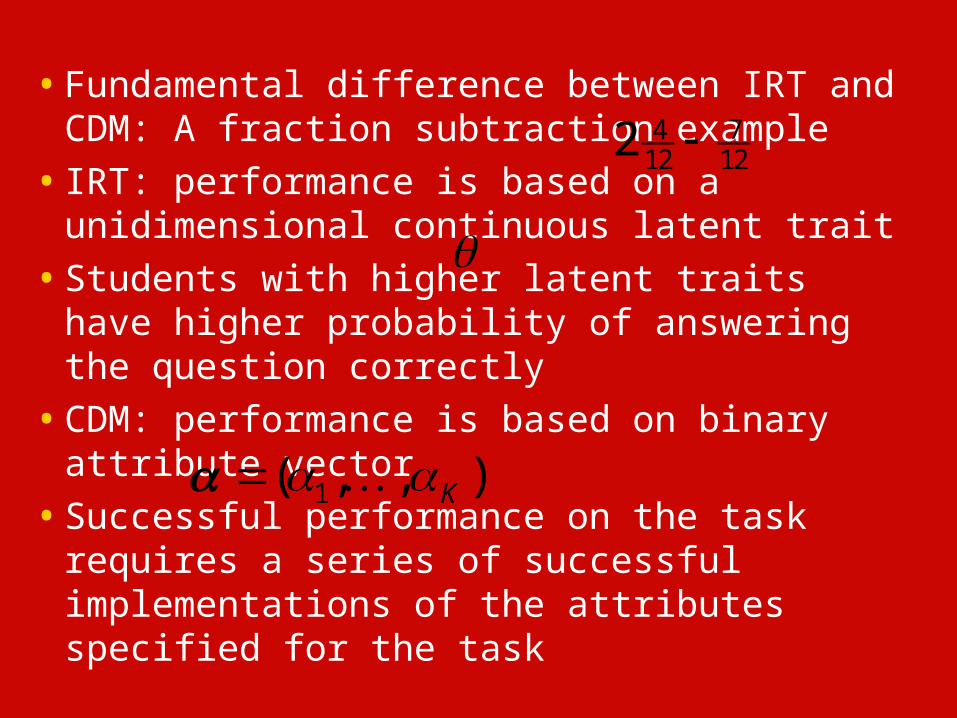
• Fundamental difference between IRT and CDM: A fraction subtraction example

• IRT: performance is based on a unidimensional continuous latent trait

• Students with higher latent traits have higher probability of answering the question correctly

7412 122

0.00

0.20

0.40

0.60

0.80

1.00

-3.5 -2.5 -1.5 -0.5 0.5 1.5 2.5 3.5

( 1| 0.8) 0.3P X

( 1| 1.2) 0.9P X

0.8 1.2

• Fundamental difference between IRT and CDM: A fraction subtraction example

• IRT: performance is based on a unidimensional continuous latent trait

• Students with higher latent traits have higher probability of answering the question correctly

• CDM: performance is based on binary attribute vector

• Successful performance on the task requires a series of successful implementations of the attributes specified for the task

7412 122

1( , , )K

7412 122

127

12161

1291

431

• Required attributes:

(1) Borrowing from whole(2) Basic fraction subtraction (3) Reducing

• Other attributes:

(5) Converting whole to fraction

(4) Separating whole from fraction

( 1| 1) 0.88P X

( 1| 0) 0.15P X

0.75

0.5

0.25

0

1

1 0

• Denote the response and attribute vectors of examinee i by and

• Each attribute pattern is a unique latent class; thus, K attributes define latent classes

• Attribute specification for the items can be found in the Q-matrix, a J x K binary matrix

• DINA (Deterministic Input Noisy “And” gate) is a CDM model that can be used in modeling the distribution of given

Background

• In the DINA model

• where

is the latent group classification of examinee i with respect to item j

• P(H|g) is the probability that examinees in group g will respond with h to item j

• In more conventional notation of the DINA = guessing, = slip

• Of the various test formats, multiple-choice (MC) has been widely used for its ability to sample and accommodate diverse contents

• Typical CDM analyses of MC tests involve dichotomized scores (i.e., correct/incorrect)

• The approach ignores the diagnostic insights about student difficulties and alternative conceptions in the distractors

• Wrong answers can reveal both what students know and what they do not know

• Purpose of the paper is to propose a two-component framework for maximizing the diagnostic value of MC assessments

• Component 1: Prescribes how MC options can be designed to contain more diagnostic information

• Component 2: Describes a CDM model that can exploit such information

• Viability (i.e., estimability, efficiency) of the proposed framework is evaluated using a simulation study

Component 1: Cognitively-Based MC Options• For the MC format, , where each

number represents a different option• An option is coded or cognitively-based if it is

constructed to correspond to some of the latent classes

• Each coded option has an attribute specification• Attribute specifications for non-coded options

are implicitly represented by the zero-vector

1,2, ,ij jY H

2 1K

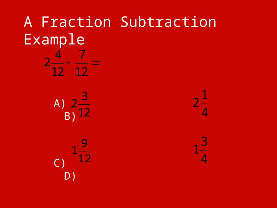
A Fraction Subtraction Example

A) B)

C) D)

4 7212 12

3212

124

31412

91

Attributes Required for Each Option of

Option

(1)

Borrowing from whole

(2)Basic

fractionsubtraction

(3)

Reducing

(4)Separating whole from

fraction

(5)Converting

whole tofraction

A)

B)

C)

D)

3212124

1291

314

4 7212 12

• The option with the largest number of required attributes is the key

Attributes Required for Each Option of

Option

(1)

Borrowing from whole

(2)Basic

fractionsubtraction

(3)

Reducing

(4)Separating whole from

fraction

(5)Converting

whole tofraction

A)

B)

C)

D)

3212124

1291

314

4 7212 12

• The option with the largest number of required attributes is the key

• Distractors are created to reflect the type of responses students who lack one or more of the required attributes for the key are likely to give

Attributes Required for Each Option of

Option

(1)

Borrowing from whole

(2)Basic

fractionsubtraction

(3)

Reducing

(4)Separating whole from

fraction

(5)Converting

whole tofraction

A)

B)

C)

D)

3212124

1291

314

4 7212 12

• The option with the largest number of required attributes is the key

• Distractors are created to reflect the type of responses students who lack one or more of the required attributes for the key are likely to give

• Knowledge states represented by the distractors should be in the subset of the knowledge state that corresponds to the key

• Number of latent classes under the proposed framework is equal to , the number of coded options plus 1

* 1jH

3D) 14

3A) 212

1B) 24

9C) 112

4 7212 12

“0”

000 001010100 011101110 111

3D) 14

3A) 212

1B) 24

9C) 112

4 7212 12

“0” “1”

000 001010100 011101110 111

3D) 14

3A) 212

1B) 24

9C) 112

4 7212 12

“2”

000 001010100 011101110 111

“3”“1”

3D) 14

3A) 212

1B) 24

9C) 112

4 7212 12

“2” “4”

000 001010100 011101110 111

“3”“1”

“0”

Component 2: The MC-DINA Model

• Let be the Q-vector for option h of item j, and

• With respect to item j, examinee i is in group

• Probability of examinee i choosing option h of item j is

' ' ' ''

arg max{ ' | ' ' }ij i jh i jh jh jhh

g q q q q

jhq0j q 0

0 and {1, , }ijg H ' 0,1, , ,h H

( | ) ( ) ( | )ij i jh i jP Y h P P h g

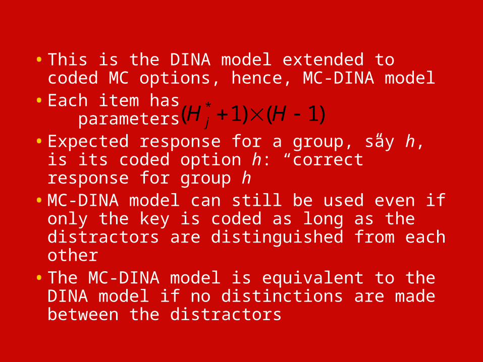
• This is the DINA model extended to coded MC options, hence, MC-DINA model

• Each item has parameters• Expected response for a group, say h, is its

coded option h: “correct” response for group h • MC-DINA model can still be used even if

only the key is coded as long as the distractors are distinguished from each other

• The MC-DINA model is equivalent to the DINA model if no distinctions are made between the distractors

*( 1) ( 1)jH H

Option

Group A B C D

0

1

2

3

4

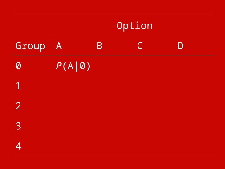
Option

Group A B C D

0 P(A|0)

1

2

3

4

Option

Group A B C D

0 P(A|0) P(B|0)

1

2

3

4

Option

Group A B C D

0 P(A|0) P(B|0) P(C|0)

1

2

3

4

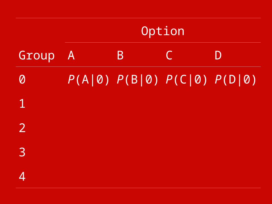
Option

Group A B C D

0 P(A|0) P(B|0) P(C|0) P(D|0)

1

2

3

4

Option

Group A B C D

0 P(A|0) P(B|0) P(C|0) P(D|0)

1 P(A|1) P(B|1) P(C|1) P(D|1)

2

3

4

Option

Group A B C D

0 P(A|0) P(B|0) P(C|0) P(D|0)

1 P(A|1) P(B|1) P(C|1) P(D|1)

2 P(A|2) P(B|2) P(C|2) P(D|2)

3 P(A|3) P(B|3) P(C|3) P(D|3)

4 P(A|4) P(B|4) P(C|4) P(D|4)

Option

Group A B C D

0

1

2

3

4

Option

Group A B C D

0

1

Option

Group A B C D

0 P(A|0) P(B|0) P(C|0) P(D|0)

1 P(A|1) P(B|1) P(C|1) P(D|1)

DINA Model for Nominal Response

N-DINA Model

Option

0

1

A B C DGroup

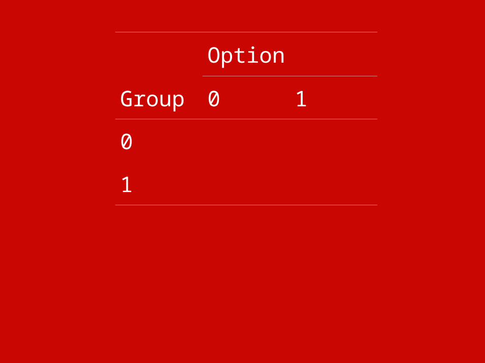
Option

Group 0 1

0

1

Option

Group 0 1

0 P(0|0) P(1|0)

1 P(0|1) P(1|1)

Plain DINA Model

P(1|0) – guessing parameterP(0|1) – slip parameter

1

111 1

11 1

( ) 1 ( )

Hijhh

ijh

XJ H HX

jh l jh lhj h

P P

, the marginalized likelihood of examinee i

Estimation

• Like in IRT, JMLE of the MC-DINA model parameters can lead to inconsistent estimates

• Using MMLE, we maximize

1 1

( ) log ( | ) ( )I L

i l li l

l L p

X X

( )iL Xprior probability of l

• Like in IRT, JMLE of the MC-DINA model parameters can lead to inconsistent estimates

• Using MMLE, we maximize

• The estimator based on an EM algorithm is

where is the expected number of examinees in group g choosing option h of item j

Estimation

1 1

( ) log ( | ) ( )I L

i l li l

l L p

X X

''( | ) ( | )1ˆ ( | ) / H

j j h g j h ghP h g I I

( | )j h gI

A Simulation Study• Purpose: To investigate how

– well the item parameters and SE can be estimated– accurately the attributes can be classified– MC-DINA compares with the traditional DINA

• 1000 examinees, 30 items, 5 attributes

• Parameters:

• Number of replicates: 100

0.25 if 0 ( | ) 0.82 if 0 and g

0.06 if 0 and gj

gP h g g h

g h

• Required attribute per item: 1, 2 or 3 (10 each)• Exhaustive hierarchically linear specification:

– One-attribute item

– Two-attribute item

– Three-attribute item

1 0 0 0 0

1 0 1 0 0

1 1 0 1 0

1 0 1 0 0 0

1 1 0 1 0 0 1 0 1 00 0

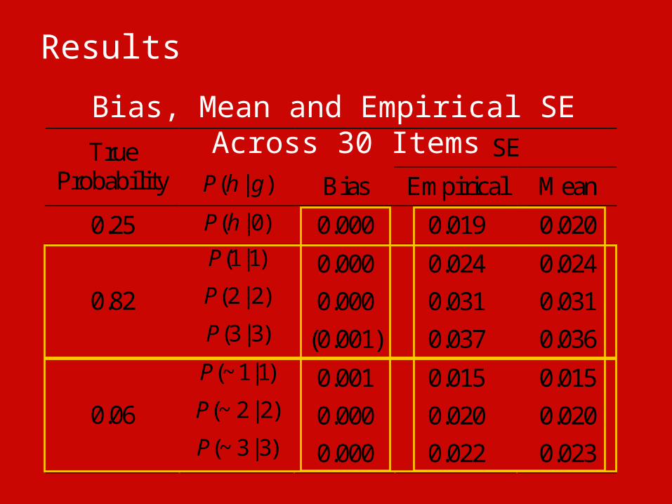
Results

Bias, Mean and Empirical SE Across 30 Items SE True

Probability ( | )P h g Bias Empirical Mean 0.25 ( | 0)P h 0.000 0.019 0.020

(1|1)P 0.000 0.024 0.024 (2 | 2)P 0.000 0.031 0.031 0.82 (3 | 3)P (0.001) 0.037 0.036

(~ 1|1)P 0.001 0.015 0.015 (~ 2 | 2)P 0.000 0.020 0.020 0.06 (~ 3 | 3)P 0.000 0.022 0.023

Bias, Mean and Empirical SE by Item Classification (True Probability: 0.25)

Item SE ( | )P h g Type Bias Empirical Mean

1 0.000 0.019 0.020 ( | 0)P h 2 0.000 0.019 0.020

3 0.000 0.020 0.020

Bias, Mean and Empirical SE by Item Classification (True Probability: 0.82)

SE ( | )P h g

Item Type Bias Empirical Mean

1 (0.001) 0.018 0.018 (1|1)P 2 0.001 0.027 0.026

3 0.000 0.026 0.026 2 0.000 0.026 0.026

(2 | 2)P 3 0.001 0.036 0.036

(3 | 3)P 3 0.001 0.037 0.036

Bias, Mean and Empirical SE by Item Classification (True Probability: 0.06)

SE ( | )P h g

Item Type Bias Empirical Mean

1 0.000 0.012 0.011 (~ 1|1)P 2 0.000 0.017 0.016

3 (0.001) 0.016 0.016 2 0.000 0.016 0.016

(~ 2 | 2)P 3 (0.001) 0.023 0.023

(~ 3 | 3)P 3 (0.001) 0.022 0.023

Review of Parameter Estimation Results

• Algorithm provides accurate estimates of the model parameters and SEs

• SE of does not depend on item type• When ,

• What factor affects the precision of ? , expected number of examinees in

group g of item j

ˆ ( | 0)jP h' 0g g

ˆ ˆ[ ( | )] [ ( | ')]j jSE P h g SE P h gˆ ( | )jP h g

( | )j gI

Illustration of the impact of

• Consider the following three items( | )j gI

Required Attributes Item 1{ } 1 2{ , } 1 2 3{ , , }

1 j

2 'j

3 ''j

{ } 1{ } 1 2{ , } 1 2 3{ , , }

j

'j

''j

( | 0)P h (1|1)P(~ 1|1)P

(2 | 2)P(~ 2 | 2)P

(3 | 3)P(~ 3 | 3)P

Implications

• The differences in sample sizes in the latent groups account for the observed differences in the SEs of the parameter estimates

• This underscores the importance, not only of the overall sample size I, but also the expected numbers of examinees in the latent groups in determining the precision of the estimates

( | )j gI

Attribute Classification Accuracy

Percent of Attribute Correctly Classified

Attribute

Model Individual Vector

MC-DINA

DINA

Difference:

97.43

91.13

6.30

89.71

69.58

20.13

Summary and Conclusion• There is an urgent need for assessments that

provide interpretative, diagnostic, highly informative, and potentially prescriptive scores

• This type of scores can inform classroom instruction and learning

• With appropriate construction, MC items can be designed to be more diagnostically informative

• Diagnostic information in MC distractors can be harnessed using the MC-DINA

• Parameters of the MC-DINA model can be accurately estimated

• MC-DINA attribute classification accuracy is dramatically better than the traditional DINA

• Caveat: This framework is only the psychometric aspect of cognitive diagnosis

• Development of cognitively diagnostic assessment is a multi-disciplinary endeavor requiring collaboration between experts from learning science, cognitive science, subject domains, didactics, psychometrics, . . .

• More general version of the model (e.g., attribute specifications need not be linear, exhaustive nor hierarchical)

• Applications to traditional MC assessments• Issues related to sample size

– Sample size needed for different numbers of items and attributes, and types of attribute specifications

– Trade-off between the number of coded options and sample size necessary for stable estimates

– Feasibility of some simplifying assumptions such as equiprobability in choosing non-expected responses

Further considerations

( | ) ( | ): , , j g j h gI I I

That’s all folks!