a class of fast algorithms for total variation image...

OpenStax-CNX module: m19059 1

A Class of Fast Algorithms for

Total Variation Image Restoration∗

Junfeng Yang

Wotao Yin

Yin Zhang

Yilun Wang

This work is produced by OpenStax-CNX and licensed under the

Creative Commons Attribution License 2.0†

Abstract

This report summarizes work done as part of the Imaging and Optimization PFUG under RiceUniversity's VIGRE program. VIGRE is a program of Vertically Integrated Grants for Research andEducation in the Mathematical Sciences under the direction of the National Science Foundation. APFUG is a group of Postdocs, Faculty, Undergraduates and Graduate students formed round the studyof a common problem.

This module is based on the recent work of Junfeng Yang ([email protected]) from NanjingUniversity and Wotao Yin, Yin Zhang, and Yilun Wang (wotao.yin, yzhang, [email protected]) fromRice University.

In image formation, the observed images are usually blurred by optical instruments and/or transfermedium and contaminated by noise, which makes image restoration a classical problem in image process-ing. Among various variational deconvolution models, those based upon total variation (TV) are knownto preserve edges and meanwhile remove unwanted ne details in an image and thus have attracted muchresearch interests since the pioneer work by Rudin, Osher and Fatemi. However, TV based models aredicult to solve due to the nondierentiability and the universal coupling of variables. In this module, wepresent, analyze and test a class of alternating minimization algorithms for reconstructing images fromblurry and noisy observations with TV-like regularization. This class of algorithms are applicable to bothsingle- and multi-channel images with either Gaussian or impulsive noise, and permit cross-channel blurswhen the underlying image has more than one channels. Numerical results are given to demonstrate theeectiveness of the proposed algorithms.

1 Introduction

In electrical engineering and computer science, image processing refers to any form of signal processing inwhich the input is an image and the output can be either an image or a set of parameters related to theimage. Generally, image processing includes image enhancement, restoration and reconstruction, edge andboundary detection, classication and segmentation, object recognition and identication, compression andcommunication, etc. Among them, image restoration is a classical problem and is generally a preprocessing

∗Version 1.2: Dec 26, 2008 10:21 am -0600†http://creativecommons.org/licenses/by/2.0/

http://cnx.org/content/m19059/1.2/


stage of higher level processing. In many applications, the measured images are degraded by blurs; e.g.the optical system in a camera lens may be out of focus, so that the incoming light is smeared out, andin astronomical imaging the incoming light in the telescope has been slightly bent by turbulence in theatmosphere. In addition, images that occur in practical applications inevitably suer from noise, which arisefrom numerous sources such as radiation scatter from the surface before the image is sensed, electrical noisein the sensor or camera, transmission errors, and bit errors as the image is digitized, etc. In such situations,the image formation process is usually modeled by the following equation

f (x) = (k ∗ u) (x) + ω (x) , x ∈ Ω, (1)

where u (x) is an unknown clean image over a region Ω ⊂ R2, ∗" denotes the convolution operation,k (x) , n (x) and f (x) are real-valued functions from R2 to R representing, respectively, convolution kernel,additive noise, and the blurry and noisy observation. Usually, the convolution process neither absorbs norgenerates optical energy, i.e.,

∫Ωk (x) dx = 1, and the additive noise has zero mean.

Deblurring or decovolution aims to recover the unknown image u (x) from f (x) and k (x) based on ((1)).When k (x) is unknown or only an estimate of it is available, recovering u (x) from f (x) is called blinddeconvolution. Throughout this module, we assume that k (x) is known and ω (x) is either Gaussian orimpulsive noise. When k (x) is equal to the Dirac delta, the recovery of u (x) becomes a pure denoisingproblem. In the rest of this section, we review the TV-based variational models for image restoration andintroduce necessary notation for analysis.

1.1 Total Variation for Image Restoration

The TV regularization was rst proposed by Rudin, Osher and Fatemi in [12] for image denoising, and thenextended to image deblurring in [11]. The TV of u is dened as

TV (u) =∫

Ω‖ ∇u (x) ‖ dx. (2)

When ∇u (x) does not exist, the TV is dened using a dual formulation [18], which is equivalent to ((2))when u is dierentiable. We point out that, in practical computation, discrete forms of regularization arealways used where dierential operators are replaced by ceratin nite dierence operators. We refer TVregularization and its variants as TV-like regularization. In comparison to Tikhonov-like regularization, thehomogeneous penalty on image smoothness in TV-like regularization can better preserve sharp edges andobject boundaries that are usually the most important features to recover. Variational models with TVregularization and `2 delity has been widely studied in image restoration; see e.g. [2], [3] and referencestherein. For `1 delity with TV regularization, its geometric properties are analyzed in [4], [16], [17]. Thesuperiority of TV over Tikhonov-like regularization was analyzed in [1], [5] for recovering images containingpiecewise smooth objects.

Besides Tikhonov and TV-like regularization, there are other well studied regularizers in the literature,e.g. the Mumford-Shah regularization [9]. In this module, we concentrate on TV-like regularization. Wederive fast algorithms, study their convergence, and examine their performance.

1.2 Discretization and Notation

As used before, we let ‖ · ‖ be the 2-norm. In practice, we always discretize an image dened on Ω, andvectorize the two-dimensional digitalized image into a long one-dimensional vector. We assume that Ω isa square region in R2. Specically, we rst discretize u (x) into a digital image represented by a matrix

U ∈ Rn×n. Then we vectorize U column by column into a vector u ∈ Rn2, i.e.

ui = Upq, i = 1, ..., n2, (3)

where ui denotes the ith component of u, Upq is the component of U at pth row and qth column, and pand q are determined by i = (q − 1)n + p and 1 ≤ q ≤ n. Other quantities such as the convolution kernel



k (x), additive noise ω (x), and the observation f (x) are all discretized correspondingly. Now we present thediscrete forms of the previously presented equations. The discrete form of ((1)) is

f = Ku+ ω, (4)

where in this case, u, ω, f ∈ Rn2are all vectors representing, respectively, the discrete forms of the original

image, additive noise and the blurry and noisy observation, and K ∈ Rn2×n2is a convolution matrix

representing the kernel k (x). The gradient ∇u (x) is replaced by certain rst-order nite dierence at pixel

i. Let Di ∈ R2×n2be a rst-order local nite dierence matrix at pixel i in horizontal and vertical directions.

E.g. when the forward nite dierence is used, we have

Diu =

ui+n − uiui+1 − ui

∈ R2, (5)

for i = 1, ..., n2 (with certain boundary conditions assumed for i > n2 − n). Then the discrete form of TVdened in ((2)) is given by

TV (u) =∑n2

i=1 ‖ Diu ‖ . (6)

We will refer to

minu

TV (u) +µ

2‖ Ku− f ‖2 (7)

with discretized TV regularization ((6)) as TV/L2. For impulsive noise, we replace the `2 delity by `1delity and refer to the resulted problem as TV/L1.

Now we introduce several more notation. For simplicity, we let∑i be the summation taken over all pixels.

The two rst-order global nite dierence operators in horizontal and vertical directions are, respectively,denoted by D(1) and D(2) which are n2-by-n2 matrices (boundary conditions are the same as those assumedon Di). As such, it is worth noting that the two-row matrix Di is formed by stacking the ith row of D(1) on

that of D(2). For vectors v1 and v2, we let v = (v1; v2) ,(v>1 , v

>2

)>, i.e. v is the vector formed by stacking

v1 on the top of v2. Similarly, we let D =(D(1);D(2)

)=((D(1)

)>,(D(2)

)>)>. Given a matrix T , we let

diag (T ) be the vector containing the elements on the diagonal of T , and F (T ) = FTF−1, where F ∈ n2×n2

is the 2D discrete Fourier transform matrix.

1.3 Existing Methods

Since TV is nonsmooth, quite a few algorithms are based on smoothing the TV term and solving an approx-imation problem. The TV of u is usually replaced by

TVε (u) =∑i

√‖ Diu ‖2 + ε, (8)

where ε > 0 is a small constant. Then the resulted approximate TV/L2 problem is smooth and manyoptimization methods are available. Among others, the simplest method is the gradient descent method aswas used in [12]. However, this method suers slow convergence especially when the iterate point is closeto the solution. Another important method is the linearized gradient method proposed in [15] for denoisingand in [14] for deblurring. Both the gradient descent and the linearized gradient methods are globally andat best linearly convergent. To obtain super linear convergence, a primal-dual based Newton method wasproposed in [13]. Both the linearized gradient method and this primal-dual method need to solve a largesystem of linear equations at each iteration. When ε is small and/or K becomes more ill-conditioned, thelinear system becomes more and more dicult to solve. Another class of well-known methods for TV/L2

are the iterative shrinkage/thresholding (IST) based methods [8]. For IST-based methods, a TV denoising



problem needs to be solved at each iteration. Also, in [6] the authors transformed the TV/L2 problem intoa second order cone program and solved it by interior point method.

2 A New Alternating Minimization Algorithm

In this section, we derive a new algorithm for the TV/L2 problem

minu

∑i ‖ Diu ‖ +µ

2 ‖ Ku− f ‖2. (9)

In ((9)), the delity term is quadratic with respect to u. Moreover, K is a convolution matrix and thus canbe easily diagonalized by fast transforms (with proper boundary conditions assumed on u). Therefore, themain diculty in solving ((9)) is caused by the nondierentiability and the universal coupling of variablesof the TV term. Our algorithm is derived from the well-known variable-splitting and penalty techniquesin optimization. First, we introduce an auxiliary variable wi ∈ R2 at pixel i to transfer Diu out of thenondierentiable term ‖ · ‖. Then we penalize the dierence between wi and Diu quadratically. As such,the auxiliary variables wi's are separable with respect to one another. For convenience, in the following welet w , [w1, ...,wn2 ]. The approximation model to ((9)) is given by

minw,u

∑i ‖ wi ‖ +β

2

∑i ‖ wi −Diu ‖2 + µ

2 ‖ Ku− f ‖2, (10)

where β 0 is a penalty parameter. It is well known that the solution of ((10)) converges to that of ((9))as β →∞. In the following, we concentrate on problem ((10)).

2.1 Basic Algorithm

The benet of ((10)) is that while either one of the two variables u and w is xed, minimizing the objectivefunction with respect to the other has a closed-form formula that we will specify below. First, for a xed u,the rst two terms in ((10)) are separable with respect to wi, and thus the minimization for w is equivalentto solving

minwi

‖ wi ‖ +β2 ‖ wi −Diu ‖2, i = 1, 2, ..., n2. (11)

It is easy to verify that the unique solutions of ((11)) are

wi = max‖ Diu ‖ − 1β , 0

Diu‖Diu‖ , i = 1, ..., n2, (12)

where the convention 0 · (0/0) = 0 is followed. On the other hand, for a xed w, ((10)) is quadratic in uand the minimizer u is given by the normal equations(∑

iD>i Di + µ

βK>K

)u =

∑iD>i wi + µ

βK>f. (13)

By noting the relation between D and Di and a reordering of variables, ((13)) can be rewritten as(D>D + µ

βK>K

)u = D>w + µ

βK>f, (14)

where

w ,

w1

w2

∈ R2n2and wj ,

(w1)j

...

(wn2)j

, j = 1, 2. (15)



The normal equation ((14)) can also be solved easily provided that proper boundary conditions are assumedon u. Since both the nite dierence operations and the convolution are not well-dened on the boundary ofu, certain boundary assumptions are needed when solving ((14)). Under the periodic boundary conditionsfor u, i.e. the 2D image u is treated as a periodic function in both horizontal and vertical directions, D(1),D(2) and K are all block circulant matrices with circulant blocks; see e.g. [10], [7]. Therefore, the Hessianmatrix on the left-hand side of ((14)) has a block circulant structure and thus can be diagonalized by the 2Ddiscrete Fourier transform F, see e.g. [7]. Using the convolution theorem of Fourier transforms, the solutionof ((14)) is given by

u = F−1

(F(D>w+(µ/β)K>f)

diag(F(D>D+(µ/β)K>K))

), (16)

where the division is implemented by componentwise. Since all quantities but w are constant for given β,computing u from ((16)) involves merely the nite dierence operation on w and two FFTs (including oneinverse FFT), once the constant quantities are computed.

Since minimizing the objective function in ((10)) with respect to either w or u is computationally inex-pensive, we solve ((10)) for a xed β by an alternating minimization scheme given below.

Algorithm :

• Input f , K and µ > 0. Given β > 0 and initialize u = f .• While not converged, Do

a. Compute w according to ((12)) for xed u.b. Compute u according to ((16)) for xed w (or equivalently w).

• End Do

2.2 Optimality Conditions and Convergence Results

To present the convergence results of Algorithm "Basic Algorithm" (Section 2.1: Basic Algorithm) for axed β, we make the following weak assumption.

Assumption 1 N (K) ∩N (D) = 0, where N (·) represents the null space of a matrix.Dene

M = D>D + µβK>K and T = DM−1D>. (17)

Furthermore, we will make use of the following two index sets:

L = i : ‖ Diu∗ ‖< 1

β and E = 1, ..., n2 \ L. (18)

Under Assumption 1, the proposed algorithm has the following convergence properties.Theorem 1 For any xed β > 0, the sequence

(wk, uk

) generated by Algorithm "Basic Algorithm"

(Section 2.1: Basic Algorithm) from any starting point(w0, u0

)converges to a solution (w∗, u∗) of ((10)).

Furthermore, the sequence satises

1.

‖ wk+1E − w∗E ‖≤

√ρ ((T 2)EE) ‖ wkE − w∗E ‖; (19)

2.‖ uk+1 − u∗‖M ≤

√ρ (TEE)‖ uk − u∗ ‖M ; (20)

for all k suciently large, where TEE = [Ti,j ]i,j∈E∪(n2+E) is a minor of T , ‖ v ‖2M= v>Mv and ρ (·) is thespectral radius of its argument.



3 Extensions to Multichannel Images and TV/L

The alternating minimization algorithm given in "A New Alternating Minimization Algorithm" (Section 2:A New Alternating Minimization Algorithm) can be extended to solve multichannel extension of ((9)) whenthe underlying image has more than one channels and TV/L1 when the additive noise is impulsive.

3.1 Multichannel image deconvolution

Let u =[u(1); ...;u(m)

]∈ Rmn2

be an m-channel image, where, for each j, u(j) ∈ Rn2represents the jth

channel. An observation of u is modeled by ((4)), in which case f =[f (1); ...; f (m)

]and ω =

[ω(1); ...;ω(m)

]have the same size and the number of channels as u, and K is a multichannel blurring operator of the form

K =

K11 K12 · · · K1m

K21 K22 · · · K2m

......

. . ....

Km1 Km2 · · · Kmm

∈ Rmn2×mn2, (21)

where Kij ∈ Rn2×n2, each diagonal submatrix Kii denes the blurring operator within the ith channel, and

each o-diagonal matrix Kij , i 6= j, denes how the jth channel aects the ith channel.The multichannel extension of ((9)) is

minu

∑i ‖ (Im ⊗Di)u ‖ +µ

2 ‖ Ku− f ‖2, (22)

where Im is the identity matrix of order m, and ⊗" is the Kronecker product. By introducing auxiliaryvariables wi ∈ R2m, i = 1, ..., n2, ((22)) is approximated by

minw,u

∑i ‖ wi ‖ +β

2

∑i ‖ wi − (Im ⊗Di)u ‖2 + µ

2 ‖ Ku− f ‖2. (23)

For xed u, the minimizer function for w is given by ((12)) in which Diu should be replaced by (Im ⊗Di)u.On the other hand, for xed w, the minimization for u is a least squares problem which is equivalent to thenormal equations (

I3 ⊗(D>D

)+ µ

βK>K

)u = (I3 ⊗D)>w + µ

βK>f, (24)

where w is a reordering of variables in a similar way as given in ((15)). Under the periodic boundarycondition, ((24)) can be block diagonalized by FFTs and then solved by a low complexity Gaussian eliminationmethod.

3.2 Deconvolution with Impulsive Noise

When the blurred image is corrupted by impulsive noise rather than Gaussian, we recover u as the minimizerof a TV/L1 problem. For simplicity, we again assume u ∈ Rn2

is a single channel image and the extension tomultichannel case can be similarly done as in "Multichannel image deconvolution" (Section 3.1: Multichannelimage deconvolution). The TV/L1 problem is

minu

∑i ‖ Diu ‖ +µ ‖ Ku− f ‖1. (25)

Since the data-delity term is also not dierentiable, in addition to w, we introduce z ∈ Rn2and add a

quadratic penalty term. The approximation problem to ((25)) is

minw,z,u

∑i

(‖ wi ‖ +β

2 ‖ wi −Diu ‖2)

+ µ(‖ z ‖1 + γ

2 ‖ z − (Ku− f) ‖2), (26)



where β, γ 0 are penalty parameters. For xed u, the minimization for w is the same as before, whilethe minimizer function for z is given by the famous one-dimensional shrinkage:

z = max|Ku− f | − 1γ , 0 · sgn (Ku− f) . (27)

On the other hand, for xed w and z, the minimization for u is a least squares problem which is equivalentto the normal equations (

D>D + µγβ K

>K)u = D>w + µγ

β K> (f + z) . (28)

Similar to previous arguments, ((28)) can be easily solved by FFTs.

4 Experiments

In this section, we present the practical implementation and numerical results of the proposed algorithms.We used two images, Man (grayscale) and Lena (color) in our experiments, see Figure 1. The two images arewidely used in the eld of image processing because they contain nice mixture of detail, at regions, shadingarea and texture.

Figure 1: Test images: Man (left, 1024×1024) and Lena (right, 512×512).

We tested several kinds of blurring kernels including Gaussian, average and motion. The additive noiseis Gaussian for TV/L2 problems and impulsive for TV/L1 problem. The quality of image is measured by



the signal-to-noise ratio (SNR) dened by

SNR , 10 ∗ log10

‖ u− E (u) ‖2

‖ u−u ‖2, (29)

where u is the original image and E (u) is the mean intensity value of u. All blurring eects were generatedusing the MATLAB function imlter " with periodic boundary conditions, and noise was added usingimnoise ". All the experiments were nished under Windows Vista Premium and MATLAB v7.6 (R2008a)running on a Lenovo laptop with an Intel Core 2 Duo CPU at 2 GHz and 2 GB of memory.

4.1 Practical Implementation

Generally, the quality of the restored image is expected to increase as β increases because the approximationproblems become closer to the original ones. However, the alternating algorithms converge slowly when βis large, which is well-known for the class of penalty methods. An eective remedy is to gradually increaseβ from a small value to a pre-specied one. Figure 2 compares the dierent convergence behaviors ofthe proposed algorithm when with and without continuation, where we used Gaussian blur of size 11 andstandard deviation 5 and added white Gaussian noise with mean zero and standard deviation 10−3.

0 500 1000 1500 2000 2500 300010

−4

10−3

10−2

10−1

100

with continuationwithout continuation

Figure 2: Continuation vs. no continuation: u∗ is an exact solution corresponding to β = 214. Thehorizontal axis represents the number of iterations, and the vertical axis is the relative error ek =‖uk − u∗ ‖ / ‖ u∗ ‖.

In this continuation framework, we compute a solution of an approximation problem which used a smallerbeta, and use the solution to warm-start the next approximation problem corresponding to a bigger β. Ascan be seen from Figure 2, with continuation on β the convergence is greatly sped up. In our experiments,we implemented the alternating minimization algorithms with continuation on β, which we call the resultingalgorithm Fast Total Variation de-convolution or FTVd, which, for TV/L2, the framework is given below.

[FTVd]:

• Input f , K and µ > 0. Given βmax > β0 > 0.• Initialize u = f , up = 0, β = β0 and ε > 0.• While β ≤ βmax, Do

a. Run Algorithm "Basic Algorithm" (Section 2.1: Basic Algorithm) until an optimality conditionis met.



b. β ← 2 ∗ β.• End Do

0 2 4 6 8 10 12 14 16 1813

14

15

16

17

18

19

20

21

22

23

log2β

SN

R (

dB)

LenaMan

Figure 3: SNRs of images recovered from () for dierent β.



Blurry&Noisy. SNR: 9.09dB FTVd: SNR: 15.55dB, t = 13.98s

(a)

Blurry&Noisy. SNR: 9.15dB FTVd: SNR: 19.25dB, t = 15.87s

(b)

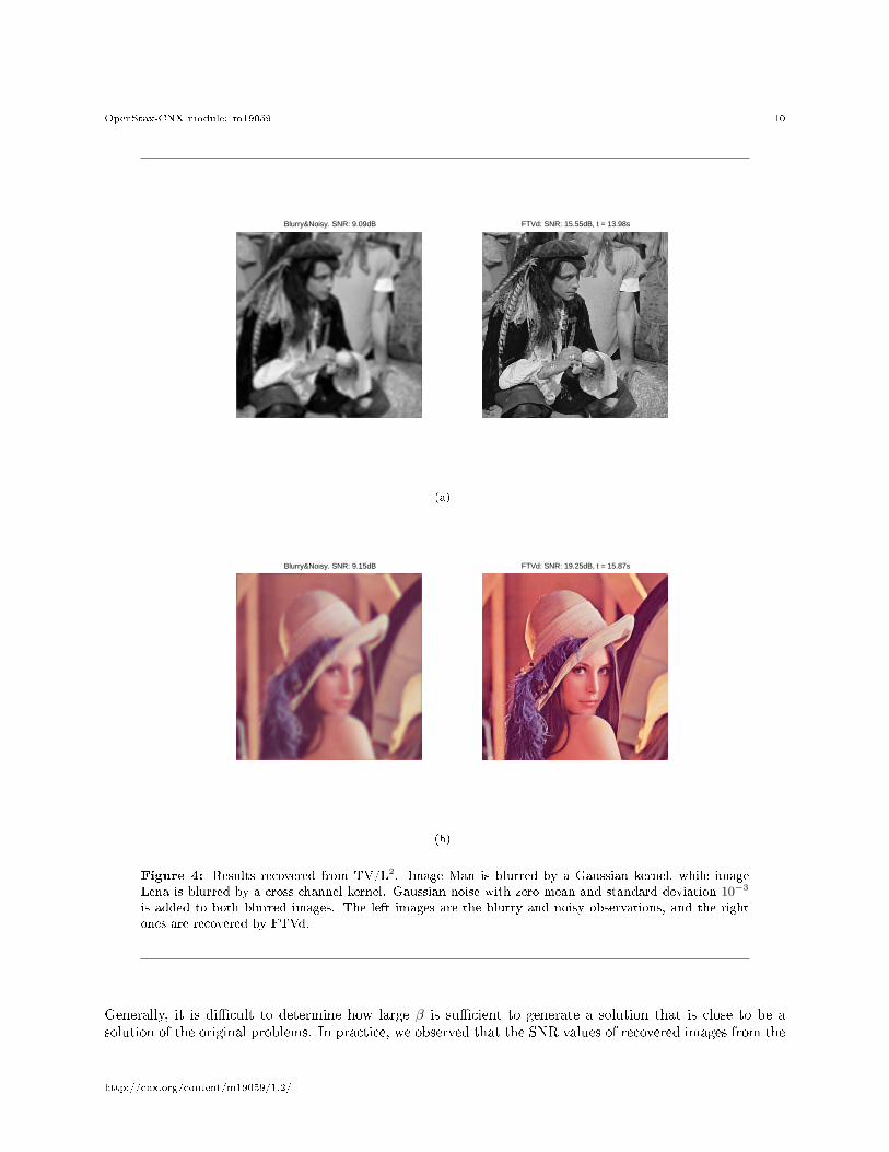
Figure 4: Results recovered from TV/L2. Image Man is blurred by a Gaussian kernel, while imageLena is blurred by a cross-channel kernel. Gaussian noise with zero mean and standard deviation 10−3

is added to both blurred images. The left images are the blurry and noisy observations, and the rightones are recovered by FTVd.

Generally, it is dicult to determine how large β is sucient to generate a solution that is close to be asolution of the original problems. In practice, we observed that the SNR values of recovered images from the



approximation problems are stabilized once β reached a reasonably large value. To see this, we plot the SNRvalues of restored images corresponding to β = 20, 21, · · · , 218 in Figure 3. In this experiment, we used thesame blur and noise as we used in the testing of continuation. As can be seen from Figure 3, the SNR valueson both images essentially remain constant for β ≥ 27. This suggests that β need not to be excessively largefrom a practical point of view. In our experiments, we set β0 = 1 and βmax = 27 in Algorithm "PracticalImplementation" (Section 4.1: Practical Implementation). For each β, the inner iteration was stopped oncean optimality condition is satised. For TV/L1 problems, we also implement continuation on γ, and usedsimilar settings as used in TV/L2.

4.2 Recovered Results

In this subsection, we present results recovered from TV/L2 and TV/L1 problems including ((9)), ((25))and their multichannel extensions. We tested various of blurs with dierent levels of Gaussian noise andimpulsive noise. Here we merely present serval test results. Figure 4 gives two examples of blurry and noisyimages and the recovered ones, where the blurred images are corrupted by Gaussian noise, while Figure 5gives the recovered results where the blurred images are corrupted by random-valued noise. For TV/L1

problems, we set γ = 215 and β = 210 in the approximation model and implemented continuation on both βand γ.



Blurry&Noisy. 30%RV Blurry&Noisy. 40%RV

(a)

Recovered. SNR: 17.98dB, t = 152s Recovered. SNR: 17.12dB, t = 234s

(b)

Figure 5: Results recovered from TV/L1. Image Lena is blurred by a cross-channel kernel and cor-rupted by 40% (left) and 50% (right) random-valued noise. The top row contains the blurry and noisyobservations and the bottom row shows the results recovered by FTVd.



5 Concluding Remarks

We proposed, analyzed and tested an alternating algorithm FTVd which for solving the TV/L2 problem. Thisalgorithm was extended to solve the TV/L1 model and their multichannel extensions by incorporating anextension of TV. Cross-channel blurs are permitted when the underlying image has more than one channels.We established strong convergence results for the algorithms and validated a continuation scheme. Numericalresults are given to demonstrate the feasibility and eciency of the proposed algorithms.

6 Acknowledgements

This Connexions module describes work conducted as part of Rice University's VIGRE program, supportedby National Science Foundation grant DMS-0739420.

References

[1] R. Acar and C.R. Vogel. Analysis of total variation penalty methods. Inv. Probl., 10:12171229, 1994.

[2] A. Chambolle and P. L. Lions. Image recovery via total variation minimization and related problems.Numer. Math., 76(2):167188, 1997.

[3] T. F. Chan, S. Esedoglu, F. Park, and A. Yip. Recent developments in total variation image restoration.CAM Report 05-01, Department of Mathematics, UCLA, 2004.

[4] T.F. Chan and S. Esedoglu. Aspects of total variation regularized function approximation. SIAM

Journal on Applied Mathematics, 65(5):18178211;1837, 2005.

[5] D. C. Dobson and F. Santosa. Recovery of blocky images from noisy and blurred data. SIAM J. Appl.

Math., 56:11818211;1198, 1996.

[6] D. Goldforb and W. Yin. Second-order cone programming methods for total variation-based imagerestoration. SIAM J. Sci. Comput., 27(2):622645, 2005.

[7] R. Gonzalez and R. Woods. Digital Image Processing. Addison-Wesley, 1992.

[8] M. Defriese I. Daubechies and C. De Mol. An iterative thresholding algorithm for linear inverse problemswith a sparsity constraint. Commun. Pure Appl. Math., LVII:14131457, 2004.

[9] D. Mumford and J. Shah. Optimal approximations by piecewise smooth functions and associatedvariational problems. Comm. Pure Appl. Math., 42:577685, 1989.

[10] Michael K. NG, Raymond H. Chan, and Wuncheung Tang. A fast algorithm for deblurring models withneumann boundary conditions. SIAM J. Sci. Comput., 21(3):8518211;866, 1999.

[11] L. Rudin and S. Osher. Total variation based image restoration with free local constraints. Proc. 1st

IEEE ICIP, 1:3135, 1994.

[12] L. Rudin, S. Osher, and E. Fatemi. Nonlinear total variation based noise removal algorithms. Phys. D,60:259268, 1992.

[13] G. H. Golub T. F. Chan and P. Mulet. A nonlinear primal dual method for total variation based imagerestoration. SIAM J. Sci. Comput., 20:19641977, 1999.

[14] C. Vogel and M. Oman. Fast, robust total variation-based reconstruction of noisy, blurred images. IEEETrans. Image processing, 7(6):8138211;824, 1998.



[15] C. R. Vogel and M. E. Oman. Iterative methods for total variation denoising. SIAM J. Sci. Comput.,17(1):227238, 1996.

[16] W. Yin, D. Goldfarb, and S. Osher. Image cartoon-texture decomposition and feature selection using thetotal variation regularized functional. In Variational, Geometric, and Level Set Methods in Computer

Vision, volume 3752 of Leture Notes in Computer Science, pages 7384. Springer, 2005.

[17] W. Yin, D. Goldfarb, and S. Osher. The total variation regularized model for multiscale decomposition.SIAM Journal on Multiscale Modeling and Simulation, 6(1):1908211;211, 2006.

[18] W. P. Ziemer. Weakly Dierentiable Functions: Sobolev Spaces and Functions of Bounded Variation.Graduate Texts in Mathematics. Springer, 1989.


a class of fast algorithms for total variation image...

Documents