ILASS-Europe 2002 Zaragoza 9 –11 September 2002

A CFD PREDICTION OF WAVE DEVELOPMENT AND DROPLET PRODUCTION ON SURFACE UNDER ULTRASONIC

EXCITATION

Yusuf Al-Suleimani and Andrew J Yule yusuf.al-suleimani@umist.ac.uk

Department of Mechanical. Aerospace and Manufacturing Engineering, UMIST, PO Box 88, Manchester M60 1QD, UK

Abstract Due to the difficulty associated with experimental investigation under ultrasonic atomization conditions, 2D and 3D CFD models were utilized to provide graphical representation of wave development and droplet production. In the 2D case 20 wave-lengths were modelled with cyclic boundary conditions, but due to computational time constraints one wave cell was modelled for the 3D case. The free surface given by the model reflected the free surface behaviour as observed in experiments, and retained an orthogonal wave pattern without liquid disintegration for low amplitude of excitation. At higher amplitude the model predicated an irregular free surface after the onset of atomization. Nomenclature a Amplitude λ Wavelength D Droplet Diameter σ Surface tension D32 Sauter mean diameter F Frequency t Time U Axial component of the velocity ρ Density µ Dynamic viscosity. Introduction Ultrasonic atomization is well known for its relatively narrow size distribution. However, this is still inadequate for some industrial applications such as manufacture of solder powder, hence the need to refine it even further. The received opinion in the literature about ultrasonic atomization is that droplets are formed periodically from the apexes of an orderly pattern of standing capillary waves, with a wavelength that can be related to vibration frequency by stability analysis. Research into exploring the physics involved goes back to 1927 when Wood and Loomis, [1], described a method of producing droplets from surfaces vibrated mechanically, as a practical means of producing sprays. Since then experimental as well as analytical work has been devoted to the study of liquid surfaces producing droplets for frequencies ranging from 20 Hz at one end of the spectrum to 5 MHz at the other end. Among those who have studied this phenomenon experimentally were Lang, [2], Pholman and Stamm, [3], Lierk and Griesshammer, [4], Topp, [5] and Sindayihebura et al., [6]. Analytical studies rely on the assumption that droplets are formed from the crests of standing capillary waves and among the leading researchers, are Lang, [2], Peskin and Raco, [7], and Sindayihebura and Bolle,[8]. Despite the numerous research projects on the physics of this phenomenon, and the theoretical confirmation that the process of ultrasonic atomization should produce a near mono-size droplet distribution, the fact remains that ultrasonic atomization of liquids can produce relatively narrow size distributions, but not a near-mono-size distribution. Reasons for this have been confirmed lately by Yule and Al-Suleimani, [9], by studying the liquid surface pre- and post-producing droplets. Their main finding was that the liquid surface, when producing droplets, loses its organized and orderly wave structure and behaves in a chaotic manner. To understand the nature of the flow of the free surface when producing droplets, CFD techniques are here employed. This is in the form of 2D and 3D Volume of Fluid computer models using the CFD code, FLUENT. Description of the Models For the results shown here, the CFD code was set up to model the vibration of a thin film of solder, as solder powder production by ultrasonic vibration, is of increasing interest in industry. The 2D computational domain was set to model 50 theoretical wave lengths calculated using the following relationship given by capillary wave theory. Here the wave length is 81.15 µm for a frequency 70kHz, as typically used in solder spraying plant.

31

2

8

=

fρπσλ

Reference should be made to Figure 1. Twenty uniformly distributed cells were assigned per wave length in the i (horizontal) direction with 35 staggered cells in the j (vertical) direction, with the finest density at the interface line between liquid and air. This was deemed adequate to give high enough resolution to show the fine details of the flow during droplet formation. The two sides of the rectangular domain were set to be periodic boundaries, meaning that liquid exiting from one side will re-enter the domain from the other side. The top gas boundary was set to be constant pressure boundary, and the height of the domain was set to be 5 times the film thickness, which was 40µm. The bottom boundary was set to “deforming wall ” , known in Fluent as “Z wall ” . The vertical deformation of this wall is governed by: )2sin( ftay π= .

The 3D model on the other hand was set to model one wave length due to computer memory limitations. Therefore the geometrical domain was in the form of a cube with square base with each side representing one wave length. The total cube height was set to be 5 times the liquid film thickness, which was set to be 40 µm. The top and bottom boundaries of the cube are similar to those prescribed in the 2D case. Unlike the 2D case FLUENT does not allow the use of periodic boundaries in the 3D model, therefore, the side walls were set to be frictionless walls, which wil l compromise the accuracy of the calculations. The computational domain has 20x20x37 cells. For both models the QUICK scheme was used to spatiall y discretize the conservation equations because of its suitability to three dimensional flow files and its greater accuracy than the other schemes. Because of the presence of free surface means that there are large spatial gradients in the pressure field, an explicit scheme of temporal discritization was used. Therefore the steep spatial gradients can be resolved, unlike for an implicit scheme that would tend to smear any large changes in the flow parameters which occur within small spatial region. The sinusoidal oscill ation was achieved by reading series of grid files positioned spatially by approximating the “sine” curve by a series of straight lines. This gives a high concentration of grid files at the peaks of the vibrations. The physical models used in the course of the calculations for both cases are: • Volume of fluid model (VOF): this has been introduced by Hirts and Nichols, [10]. This model enables

the fractional volume calculations by introducing a function F to the flow calculations, such that its value is unity at any point occupied by fluid and zero otherwise. The average value of F in a cell represents the fractional volume of the cell occupied by the fluid. Cells with F values between zero and one contain a free surface.

• Donor-Acceptor scheme (DNA): The essential idea of this scheme is to use information about F downstream as well as upstream of a flux boundary, to establish a crude interface shape, and then use this shape in computing flux. The VOF method util ises this scheme so that is uses information about the slope of the surface to improve the fluxing algorithm.

• Surface Tension model: The surface tension, as is well known, plays an important role during atomization from a free surface and simulating this force is essential for realism of the model, [11].

The 2D model was run without imposing any initial disturbance to the free surface. While the 3D model was prescribed with an initial wave profile with trough at the centre of the computational domain. Results and Discussion Figure 1 presents the film interface solder for time steps of the 2D Model. As can be seen from the images, the experimentally observed surface chaos, [9], is evident as more droplets are formed. The computational time step corresponds to 0.486 µs and TS, in Figure 1, is the total number of time steps of the computation. In order to see the velocity field, the waves a portion of the domain was enlarged and superimposed with the interface of air/solder line, as shown in Figure 2. It is clear that the liquid contained in the developing ligament is moving upwards while the gas around it has a downward velocity. This downward velocity is responsible or suppressing the development of the wave. Unless the wave has high enough energy to overcome this resistance it may not travel high enough hence, drawing back without producing any droplet. This is evident at the pair of waves at the left in figure 2, where the gas downward velocity is high (29.7 m/s), these waves could not stretch high enough to produce even a fully grown ligament. Examples of 3D model results are shown in Figure 3a-d for a vibration ampli tude of 5µm, which is not sufficient to give drop formation. The amplitude was increased to 7µm (near the critical value) and typical results are shown in Figs 4-7. Despite the non-physical behaviour of the free surface near the walls, the velocity flow fields during the process of centralised droplet formation give a good indication of what truly happens within the liquid film during this process. An initial examination of the results given with the 7 µm ampli tude shows that the free surface behaves more realistically. The first notable feature of the simulation, occurs during the second oscil lation of the deforming

(1)

wall and is a central wave peak. However, the energy of this wave peak is not sufficient to release a droplet an it is subsequently falls back towards the level position. The behaviour of the velocity field during this descendency of the central wave peak is with recirculation zones driving the free surface downwards in the centre and upwards near the frictionless walls. The descendent of the wave peak into a trough progresses with the trough actually reaching the wall . As the trough then begins to ascend, with the recirculation zones reversed, an entrained bubble is deposited on the wall and it remains in place since there are no buoyancy terms included in the transport equations. As the wave peak rises this time there is enough momentum contained within it to release a droplet. The highest velocities exist in the centre of the wave peak with the liquid near its surface being slowed by surface tension. As this develops further the liquid at the top of the wave peak reaches its maximum height and is almost stationary whereas the 'neck' of the wave peak contains liquid which continues to rise towards the top, Figure 5. This results in an accumulation of liquid at the top of the wave peak which then starts to bulge into a 'head'. As the wall moves downwards and pulls the bulk liquid film with it, the head and part of the neck of the wave detaches from the liquid film, figure 8, to form a ligament. Difference in the velocity field in the ligament cause to break-up into a main droplet (D ≈28 µm) and a satell ite droplet (D ≈13 µm). It is worth noting that the diameter of the main droplet is almost exactly one third of the capill ary wavelength and this agrees very closely with Lang's equation (1). Surface tension then acts on both of these droplets which gives them more sphericity as time progresses, figure 7. Acknowledgments The authors acknowledge the contribution by A. Coll ins. References [1] Wood, R. W., and Loomis, A. L., “The physical effects of high-frequency sound waves of great intensity” ,

Phil. Mag. 7, 417-433, (1927) [2] Lang, R. J.,“Ultrasonic atomization of liquids. J. Acoust. Soc. Am. 34, 6-9, (1962). [3] Pohlman, R., and Stamm, K., “Untersuchung zum mechanismus der ultraschallvernebelung an

fluessigkeitsoberflaechen im hinblick auf technische anwendungen” , Forschungsber, Landes Nordrhein-Westfalien 1480, 1–5, (1965)

[4] Lierke, E. G., and Griesshammer, G., “The formation of metal powders by ultrasonic atomization of molten metals” , Ultrasonics (October), pp. 224–228, (1967).

[5] Topp, M. N., “Ultrasonic atomization—a photographic study of the mechanism of disintegration” , Aerosol Sci. 4, 17–25, (1973).

[6] Sindayihebura, D., Cousin, J., and Dumouchel, C., “Experimental and theoretical study of sprays produced by ultrasonic atomizers” , Part. Part. Sys. Charact. 14, 93–101, (1997).

[7] Peskin, R. L., and Raco, R. J., “Ultrasonic atomization of liquids” , J. Acoust. Soc. Am. 35, 1378-1381, (1963).

[8] Sindayihebura, D., and Bolle, L., “Ultrasonic atomization of liquids: stabili ty analysis of the viscous liquid film free surface”, Atomization Sprays 8, 217–233, (1998).

[9] Yule, A. J., and Al-Suleimani, Y., “On droplet formation from capill ary waves on a vibrating surface”, Proc. Roy. Soc. London., A 456, 1069- 1085, (2000).

[10] Hirt, C. W., and Nichols, B. D., “Volume of Fluid (VOF) Method for the dynamics of free boundaries” , The Journal of Computational Physics. 39, 201-225, (1981).

[11] Brackbill , J. U., Koth, D. B., and Zemach, C., “A continuum method of modell ing surface tension” , The Journal of Computational Physics. 100, 335-354, (1959).

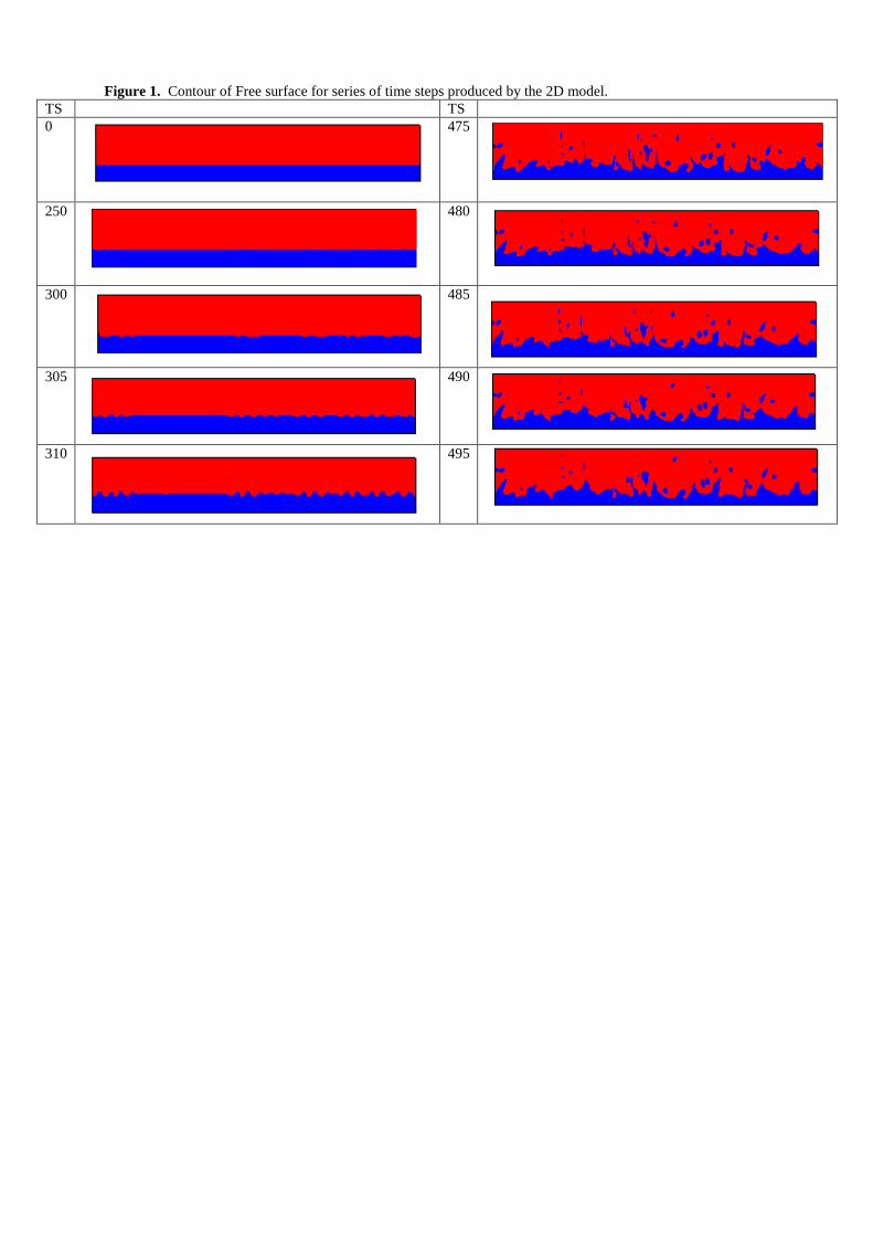
Figure 1. Contour of Free surface for series of time steps produced by the 2D model. TS TS 0

475

250

480

300

485

305

490

310

495

Figure 2. Velocity vector field showing solder (yellow) and interface.

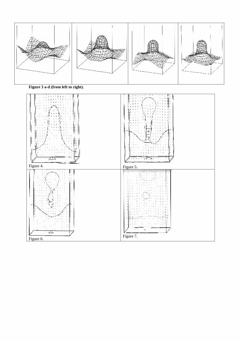
Figure 3 a-d (from left to right).

Figure 4.

Figure 5.

Figure 6.

Figure 7.