a cfd framework for analysis of helicopter · pdf filea cfd framework for analysis of...

A CFD Framework for Analysis of Helicopter Rotors

R. Steijl∗, G.N. Barakos†and K.J. Badcock‡

University of Glasgow, Glasgow G12 8QQ, United Kingdom

A CFD method suitable for the analysis of hovering and forward-flying rotors has beendeveloped and validated against experimental data. The Caradonna and Tung as wellas the ONERA 7A/7AD1 rotors have been simulated and results were found to be inexcellent agreement with wind tunnel measurements. As a second step the method wascoupled with a trimming algorithm devised using rotor blade element theory. The coupledalgorithm demonstrates the rapid convergence to prescribed thrust coefficient values andno deterioration of the convergence rates relative to simulations of untrimmed rotors.

I. Introduction

During the last decades, CFD methods for the numerical simulation of the flow around fixed-wing aircrafthave improved significantly.1 Modern CFD methods can with relative ease, at design conditions, predictwith good accuracy wing lift and with fair accuracy total wing drag. For rotary-wing aircraft, however, thesituation appears to be more complicated and the application of CFD in the rotorcraft industry has notreached the same level of maturity. It appears that CFD analysis of flows around rotary-wing aircraft issignificantly harder in comparison to the fixed-wing case.2–10 There are several reasons contributing to thissituation: i) Rotor flows are complicated and rich in fluid mechanics phenomena.11 CFD methods have tocope with strong interacting vortices, the formation of a vortex wake that spirals down below the rotor disk,transition to turbulence and a wide variation of the Mach and Reynolds numbers in the radial direction andaround the azimuth. ii) There is a strong link between the aerodynamics and aeromechanics for rotor flows.This includes both the ’rigid blade’ motions of the rotor blades about hinges in the rotor hub and the elasticdeformation of the rotor blades. In level forward flight, the rotor blade motions form part of the problem, asare the control setting of the rotor to achieve the required flight state. This is known as the rotor trimmingproblem which further complicates the numerical simulations of the flow field created by a rotor in forwardflight.Figure 1 introduces the frame of reference used here, i.e. the rotor shaft axis is the z-axis and the rotorrevolves in anti-clockwise direction. The angle ψ defines the azimuthal position. The coordinate systemx corresponds to the helicopter-fixed frame of reference. In this system, the rotor moves in the negativex-direction. For a typical helicopter rotor, the rotor blades are attached to the rotor head by a set of threehinges: the flap hinge allowing the blade to flap up and down, the lead-lag hinge allowing the blade an in-plane forward or backward motion and the feathering hinge, required to change the blade pitch. In a numberof modern helicopters one or more of these hinges is replaced by a flexible connecting beam. The degrees offreedom about the hinges are necessary for achieving a balance of forces and moment on the helicopter. Theconstruction of rotor heads is fully explained in many text books.12–14 A rotor with these degrees of freedomfor the blades is called fully articulated. Figure 1 shows the linear transformations from the helicopter-fixedframe of reference to a blade-fixed frame of reference. The control input consists of a ’collective’ pitch,i.e. a revolution averaged pitch that is identical for all blades, and a ’cyclic’ pitch, i.e. a periodic pitchchange in the azimuthal direction. The deflections in flapping and lead-lag result from balances of inertialand aerodynamic forces. In the case of hover, the blade encounters a constant blade normal velocity, andas a result, no cyclic pitch change is needed to balance the helicopter. In this case, a cyclic pitch is set

∗Postdoctoral research assistant, Computational Fluid Dynamics Laboratory, Department of Aerospace Engineering. email:[email protected]

†Lecturer, Computational Fluid Dynamics Laboratory, Department of Aerospace Engineering. email:[email protected]

‡Reader, Computational Fluid Dynamics Laboratory, Department of Aerospace Engineering. email: [email protected]

1 of 14

American Institute of Aeronautics and Astronautics

and a constant flapping deflection (’coning’) results. In forward flight, the blades experience a blade normalvelocity that depends on the azimuthal position. For a radial station r/R of a rotor blade, the blade normalMach number is

Mn(ψ) = Mtipr

R+M∞ sinψ = Mtip

( r

R+ µ sinψ

)

where µ = M∞/Mtip is the advance ratio of the rotor.Level forward flight of a helicopter requires that the rotor generates the required upward and forward

thrust, while at the same time having no rolling or pitch-up moment. Assuming that the rotor creates forcesnormal to the tip-path plane, this plane is tilted forward to create the needed forward thrust. A level forwardflight of a helicopter involves the following unknowns: the forward tilt of the tip-path plane, the collectivepitch, cyclic pitch and flapping and lead-lag harmonics. Obtaining these is part of the trimming problem.The main objective of this work is to present and validate all the extensions necessary to convert a CFDmethod for ”fixed-wing” aircraft aerodynamics to a CFD code capable of simulating a helicopter rotor inhover and in (trimmed) forward flight.The simulation of a trimmed rotor in forward flight is far more challenging than the hover problem, both interms of the problem formulation and the CPU requirements.The extensions of the CFD method for rotorcraft applications include: i) a hover model which treats theflow as a steady problem in a non-inertial frame of reference2,15 ii) a forward-flight formulation whichsolves the governing equations in a fixed inertial frame of reference accounting for isolated helicopter rotorswith fully-articulated blades (i.e. the blades carry out periodic flap, lead-lag and pitch motions) iii) a mesh-deformation technique that deforms a multi-block structured mesh to account for these rotor blade deflectionsusing a combination of rigid mesh motion (mesh blocks attached to a blade move with that blade) and griddeformation. The deformation method is based on the Trans-Finite Interpolation (TFI) method. Finally atrimming algorithm for forward-flight simulations is necessary. This is a basic trimming method based onblade element theory and approximate blade flapping equations.13 The method uses the loads on the bladesfrom the CFD solution. The extensions for rotorcraft applications are included in a CFD solver previouslyused for various applications, including fixed-wing applications and aero-elastic analysis.1

II. Description of numerical method

In order to solve problems in time dependent domains, including moving boundaries, the Navier-Stokesequations are used in the arbitrary Lagrangian Eulerian (ALE) formulation. For any control volume V withboundary ∂V and outward unit normal ~n, the conservation laws can be written in integral form as:

d

dt

∫

V (t)

~wdV +

∫

∂V (t)

(

~F (~w) − ~Fv(~w))

~ndS = ~S (1)

where ~w is the vector of conserved variables, ~F and ~Fv are the inviscid and viscous flux, respectively. In theabsence of volume forces and in an integral frame of reference source ~S = 0. A block-structured cell-centredfinite-volume method based on curvilinear boundary-fitted meshes is used here. The spatial discretisation ofEquation (1) leads to a set of ordinary differential equations in time,

d

dt

(

wi,j,kVi,j,k

)

= −Ri,j,k

(

w)

(2)

where w and R are the vectors of cell averaged conserved variables and residuals, respectively. Here, i, j, kare the cells indices in each of the grid blocks. In Equation (2), Vi,j,k is the cell volume. The convective termsare discretised using Osher’s upwind scheme.16 MUSCL variable interpolation is used to provide third-orderaccuracy with the Van Albada limiter to prevent spurious oscillations. Boundary conditions are set by usingghost cells on the exterior of the computational domain. In the far field, ghost cells are set at the free-streamconditions. For the present inviscid flow simulations, ghost values are extrapolated from the interior at solidboundaries ensuring the normal component of the velocity on the solid wall is zero.

For the present time-accurate simulations, temporal integration is performed using an implicit dual-timestepping method. Following the pseudo-time formulation,17 the updated mean flow solution is calculated bysolving the steady state problems

R∗

i,j,k =3V n+1

i,j,k wn+1i,j,k − 4V n

i,j,kwni,j,k + V n−1

i,j,k wn−1i,j,k

2V n+1i,j,k ∆t

+Ri,j,k

(

wn+1i,j,k

)

V n+1i,j,k

= 0 (3)

2 of 14


where the terms V n−1i,j,k , V n

i,j,k and V n+1i,j,k represent the cell volume at different (real) time steps. Equation (3)

represents a nonlinear system of equations. This system can be solved by introducing an iteration throughpseudo time τ to the steady state, as given by

wn+1,m+1i,j,k − w

n+1,mi,j,k

∆τ+

3V n+1i,j,k w

n+1,mi,j,k − 4V n

i,j,kwni,j,k + V n−1

i,j,k wn−1i,j,k

2V n+1i,j,k ∆t

+ Ri,j,k

(

wn+1,mi,j,k

)

V n+1i,j,k = 0 (4)

where the m-th pseudo-time iterate at real time step n + 1 is denoted by wn+1,m. The unknown wn+1i,j,k is

obtained when Equation (4) converges in pseudo-time to a specified tolerance. Typically the pseudo-timeintegration in Equation (4) is continued at each real time step until the residual has dropped three ordersof magnitude. For the simulations presented here, this typically required 25 − 35 pseudo-time steps. Animplicit scheme is used for the pseudo-time integration. The resulting linear system of equations is solvedusing the Generalised Conjugate Gradient method.18

A. Hover Modelling

Assuming that the shed wake from the rotor is steady, the hover problem can be re-cast in a steady state form.For a rotor-fixed frame of reference, the Navier-Stokes equations of Equation (1) can be used with the meshvelocity set to zero everywhere and a source term accounting for centripetal and Coriolis acceleration. Inthis non-inertial frame of reference, the energy equation needs to be modified to only account for the velocitycontributions relative to the rigid-body rotation. This relative velocity field is ~ur. In the undisturbedsituation, ~ur = −~ω×~r, where r is the position vector of the considered point and ~ω = [0, 0, ωz]

T the rotationvector of the rotor. This creates difficulties in imposing boundary conditions, i.e. the ’far-field’ has anundisturbed velocity field that depends on the position of the considered point relative to the rotation axis.In the present formulation, a non-inertial frame15 is used that resolves these problems. The frame of referenceis created by introducing a grid velocity −~ω×~r. Relative to this frame of reference the velocity ~uh = ~ur+~ω×~ris defined. Using this non-inertial frame of reference, the governing equations are given by Equation (1) withnon-zero mesh velocities and source vector S defined as:

~S =[

0,−ω × ~uh, 0]T

(5)

This results in a small source term for the momentum equations, the energy equations is unchanged. Hoversimulations typically involve only one rotor blade and periodic boundary conditions to model the presenceof the remaining blades. In the present work, the rotor shaft coincides with the z-axis and the rotorspanwise direction corresponds to the x-axis, though all possible configurations can be treated. Two differentapproaches to impose far-field boundary conditions are used. The first is based on imposing unperturbedfree-stream conditions at the far-field of the computational domain with extrapolation used in the verticaldirection on the inflow and outflow boundaries for all variables. Experience shows that the far-field boundariesneed to be at least 5 rotor radii away from the rotor when using this far-field boundary condition. A smallerdomain leads to a significant re-circulation of the flow within the domain. The second approach is termed as’potential sink’ or ’Froude’ boundary condition and is designed to suppress this re-circulation by placing apotential sink at the rotor origin.2,4, 6 Furthermore, based on actuator-disk theory, a constant axial (outflow)velocity is prescribed on a circular part of the outflow boundary face. The magnitude of this velocity isdetermined by the rotor thrust (which gives the induced axial velocity through the rotor disk according toactuator-disk theory) and the outflow radius, for which the following empirical relation4 is used:

Routflow

R= 0.78 + 0.22 exp(−doutflow/R) (6)

where doutflow is the distance of the outflow boundary below the rotor disk. Actuator-disk theory predictsa wake contraction to R/

√2 far from the disk, where the axial velocity is twice the induced axial velocity

through the rotor disk. Here, doutflow/R ≈ 4 and Routflow/R ≈ 0.783. On the remainder of the far-fieldboundary, the velocity due to the potential sink is imposed. The strength of the sink is chosen to balancethe mass flow into and out of the computational domain.

B. Forward Flight Modelling

The simulation of a helicopter rotor in forward flight requires a balance of moments and forces that isachieved by: i) tilting the rotor shaft forward and selecting a ’collective’ blade pitch so that the rotor

3 of 14


forward thrust balances the drag and the vertical thrust the weight ii) introducing ’cyclic’ pitch angles (i.e.harmonic pitch variations) that reduces the pitch on the advancing side where the blades experiences highvelocities and increases the pitch on the retreating side iii) the flapping and lead-lag degrees of freedom willresult in periodic flapping and lead-lag blade motions. The trimming problems consists of finding the rotorshaft angle, ’collective’ pitch and ’cyclic’ pitch angles that result in steady level flight. Modeling a trimmedhelicopter rotor in forward flight therefore requires: i) a method to introduce the rotor blade settings andperiodic motions ii) a method that adapts the grid to account for these blade motions iii) a trimming methodthat determines the harmonic coefficients of the blade motions. The present forward flight model is describedin more detail elsewhere.19 In the present work, the rotor blade flapping, lead-lag and pitching are assumedto be described by the negative Fourier series commonly used in rotorcraft analysis:

ψ = ωt

β(ψ) = β0 − β1s sin(ψ) − β1c − cos(ψ) − . . .

δ(ψ) = δ0 − δ1s sin(ψ) − δ1c cos(ψ) − . . . (7)

θ(ψ) = θ0 − θ1s sin(ψ) − θ1c cos(ψ) − . . .

where ω is the constant rate of rotation about the z-axis. The collective pitch is θ0 and the coning angle isβ0. In the present work, only the first harmonic is used. Assuming a constant rotation rate of the rotor, thetemporal derivatives of the flap angle, lead-lag angle and pitch angle can be written as

dβ

dt= ω

dβ

dψ;

dδ

dt= ω

dδ

dψ;

dθ

dt= ω

dθ

dψ. (8)

In the present model, the flow is solved in the ’helicopter-fixed’ frame of reference, i.e. the forward motionis modeled by introducing a free-stream velocity. Figure 1 defines the frame of reference for the rotor inforward flight and the linear transformations connecting the helicopter-fixed frame of reference to a bladefixed frame of reference. The coordinates of a point P in terms of the helicopter-fixed frame of referenceafter rotation (ψ), flapping (β), lead-lag (δ) and pitching (θ) become:

~xP = CrotCflapClagCpitch

(

~xP − ~xpitch

)

+ CrotCflapClag

(

~xpitch − ~xlag

)

+

CrotCflap

(

~xlag − ~xflap

)

+ Crot~xflap (9)

where ~xflap, ~xlag and ~xpitch defined the locations of the flap hinge, lead-lag hinge and the pitch centre andCrot, Cflap, Clag and Cpitch are the linear transformation matrices for the rotor rotation, blade flapping,blade lead-lag and blade pitching, respectively. The velocity of P in terms of the helicopter-fixed frame ofreference is obtained by taking the derivative of Equation (9). In the present method, a novel method isused to account for the rotor blade motions.19 The multi-block grid is divided in blocks that are selectedto mode rigidly with one of the rotor blades and the remaining blocks that are deformed to account for the’rigid’ motion of the surrounding blocks. The method can be summarized as follows: i) Blocks connectedto the rotor blade are tagged to move ’rigidly’. For each of these blocks the corresponding blade number isstored. ii) For the remaining blocks the number of connections to ’rigid’ moving blocks is determined. iii)For the remaining blocks that have 2 connections to ’rigid’ moving blocks, these are also tagged to move’rigidly’. This will fill the remaining ’gaps’ to form a layer of blocks around the rotor blades with a smoothbounding surface. iv) For the blocks tagged to move ’rigidly’, the grid in the initial position (ψ = 0o) is storedfor reference. This block selection strategy is shown in Figure 2, which shows a close-up of the multiblocktopology of the grid for one blade of the 4-bladed 7A20 model rotor. The shaded surface forms the boundingsurface of the grid blocks that are automatically selected to move with the rotor blade. The grid outside ofthis shaded surface is deformed using the Transfinite Interpolation method. Equation (9) is used to updatethe grid from time level n to n+ 1 for the blocks tagged for rigid-mesh motion. The method to update thegrid for the blocks not moving with one of the rotor blades from time level n to n + 1 starts by selectingblock faces connected to ’rigid’ moving blocks and updating the mesh for these block faces using Equation(9). Then, the effect of rotor rotation is subtracted from the mesh updates and the block face updates arepassed to the Transfinite Interpolation routine. After applying the Transfinite Interpolation method, thedeformed mesh is rotated to the new azimuth.

4 of 14


C. Trimming method

In this work, the trimming method is based on blade-element theory.12–14 The trimming method consistsof an initial trim-state computation and a number of subsequent re-trimming steps. Due to the simplenature of the method, the initial trim-state cannot be expected to be very accurate. In the re-trimmingsteps, the actual loads on the blade from the CFD solution are used to update the collective pitch in aNewton-Raphson process. In simulations of trimmed hovering rotors, the re-trimming is carried out afterthe steady flow solutions has converged to a prescribed level. The-trimming is repeated every nretrim steps.In simulations of trimmed forward flying rotors, revolution-averaged integrated loads from the CFD solutionare used. The trimming method needs a target thrust as input and a model for the fuselage and its dragis necessary to compute the total drag as a function of the helicopter advance ratio µ. Table 1 summarizesthe trimming approach used in the present work for hovering rotors as well as rotors in forward flight. Thesketches in Table 1 define the tip-path plane and the no-feathering plane within the rotor shaft frame ofreference.

III. Results for hovering helicopter rotors

A. Model rotor test cases

The Caradonna and Tung21 and the HELISHAPE 7A/7AD1 rotors20 have been used as validation hovertest cases. Results for these rotors are compared to wind tunnel data in this section. A summary of thehover cases is given in Table 2. Figure 3 presents the planform of the model rotors. The Caradonna andTung model rotor employed two cantilever-mounted, manually adjustable blades. The blades have a NACA0012 profile and are untwisted and untapered. The rotor aspect ratio, defined as the ratio of rotor radiusand blade chord, is 6. The model rotor has a diameter of 2.286m, and a chord length of 0.191m. Two casesfor this rotor are considered: 0o blade pitch incidence (non-lifting condition) and 8o blade pitch.The 7A/7AD1 model rotors were tested in the DNW wind tunnel during the HELISHAPE research cam-paign.20 It is a 4-bladed rotor with 2.1 m radius, 0.14 m chord and has a non-constant geometric twist. Therotor has a rectangular planform and consists of ONERA OA213 and OA209 aerofoil sections. The rotorblade aspect ratio is 15. Figure 4 compares the computed chordwise surface pressure distribution for theCaradonna and Tung model rotor with the experimental data for 3 radial sections (r/R = 0.68, r/R = 0.80and r/R = 0.89). The agreement is very good for both lifting and non-lifting cases.Figure 5 compares the computed chordwise surface pressure distribution for the HELISHAPE 7A/7AD1model rotors with the experimental data for 3 radial sections (r/R = 0.50, r/R = 0.915 and r/R = 0.975)and for both tip geometries, the agreement with the experimental data is very good. The scatter in theexperimental for the 7A rotor is due to the fact that measurements from multiple blades of the wind tunnelmodel were combined, showing differences from blade to blade. The results for the 7A/7AD1 rotors indicatethat with the present CFD method, even on the relatively coarse meshes used here, the surface pressure ontwisted blades at realistic tip Mach numbers can be predicted with a good level of accuracy. Furthermore, theresults for the 7AD1 rotor show that the present multi-block topology can be used to mesh even complicatedtip shapes (see Figure 3 for a description of the 7AD1 planform).

B. Trimmed Rotor Cases

For a hovering rotor, the trimming problem for a rigid rotor consists of finding a collective pitch that willproduce the required rotor thrust T at a fixed rotor rotation rate (i.e. fixed tip Mach number). The thrustis normalized here as: CT = T/(ρu2

tipπR2), where CT is the thrust coefficient and R the rotor radius. As a

result of the flapping degree of freedom, the rotor blade settle at a constant flapping deflection, giving therotor a coning angle at which the moments are balanced about the flap hinges.Figure 6 shows sample results for the ONERA 7A model rotor in hover. The plots compare results based onthe initial trim approximation and results obtained using a re-trimming after every 250 iterations. The gridused in the simulations has a built-in collective pitch of 7.5o at 0.7 of the rotor radius and 0o built-in coning.

Figure 6(a) shows the result for a target CT = 0.0050, which requires a reduction of the collective pitchrelative to the built-in collective pitch. The initial trimming over-predicts the collective pitch, i.e. the resultwithout subsequent re-trimming converges to a CT value above 0.0050. The re-trimming leads to a step-wisereduction in the collective pitch, until converging to a value 1.5o lower than the built-in collective pitch,

5 of 14


y

roto

r sh

aft

z

shaft−normal plane

tip−path plane

x

β1c

no−feathering plane

θ 1s

flight direction

y

x

z

shaft−normal plane

tip−path plane

no−feathering planeθ 1sβ 1c

flight direction

roto

r sh

aft

shaft− θ

1c shafttppβ = θ − θ

Table 1. Trimming approach for forward flight and hover

Forward flight Hover

1) tip-path plane orientation θtpp = −D/W θtpp = 0

2) determine inflow factor λ = µθtpp + λi λ = λi

3) determine induced inflow λi from iteration: λi = −√

CT

2

λi = − cT

21

√

µ2+(

µ sin θtpp+λi

)

2

4) estimate for collective cT

σ = a4

[

23θ0

1−µ2+9µ4/41+3µ2/4 + λ 1−µ2

1+3µ2/4

]

θ0 = 6σaCT + 3

2

√

CT

2

5) approximate flapping equation β0 = γ8

[

θ0(

1 + µ2)

+ 43λ− 4

3µβ(nfp)1c

]

β0 = γ8

[

θ0 + 43λ]

(relative to no-feathering plane) β(nfp)1c =

µ

(

8

3θ0+2λ

)

1+ 3

2µ2

β1c = 0

β(nfp)1s =

4

3µβ0

1+ 1

2µ2

β1s = 0

6) assume blade flapping β1c = θtpp − θshaft n.a.

β1c = 0 n.a.

7) determine cyclics θ1s = β(nfp)1c − β1c n.a.

θ1c = −β(nfp)1s + β1s n.a.

8) rotor loads from CFD compute δθ0 compute δθ0

repeat steps 1-8 repeat step 2-5, 8

CT = T/(ρu2tipπR

2), σ = NbladescπR , γ = ρacR4

I , a (lift-slope factor), I (moment of inertia)

Table 2. Summary of conditions for the hovering Caradonna-Tung and HELISHAPE 7A/7AD1 rotors.

Flow Conditions Caradonna-Tung21 Caradonna-Tung21 7A20 7AD120

Tip Mach Number Mtip 0.520 0.439 0.6612 0.6612

Reynolds Number 2.3 · 106 1.9 · 106 2.1 · 106 2.1 · 106

Collective pitch θc 0o 8o θ0.7 = 7.5o θ0.7 = 7.5o

Computation Details

Grid Size (periodic) 1.1 · 106 2.0 · 106 0.6 · 106 0.6 · 106 and 1.3 · 106

Modelling Inviscid Inviscid Inviscid Inviscid

6 of 14


while the coning angle converges to a value of 1.3o. Results for a target CT = 0.0068, which is close tothe experimental value obtained in the HELISHAPE campaign for the built-in collective and the tip Machnumber 0.6612 used here, are shown in Figure 6(b). Again, the initial trimming over-predicts the collectivepitch. The re-trimming leads to a CT that matches the target value at a collective pitch angle 0.35o largerthan the built-in collective pitch. At convergence, the coning angle is 2.3o. The dashed line in Figure 6 showsthe convergence of the thrust coefficient without any trimming. As can be seen, the overhead of the presenttrimming algorithm in comparison to a hover calculation without trimming at a given set of collective andconing angles is moderate. An increase between 50 % and 70% in the number of iterations is observed.

IV. Results for helicopter rotors in forward flight

A. Non-lifting ONERA model rotor in high-speed forward flight

Figure 7 shows the geometrical definition of the non-lifting 2-bladed model rotor tested at ONERA.22,23

Two different rotor blade configurations are considered here. One has a nearly straight leading edge and a75 cm radius, while a second configuration has 30o leading edge sweep on the outer 15% and has a radiusof 83.5 cm. The blades used here are different from the ONERA experiment in that the tapered root partsof the blades are removed. i.e. the blade up to 37% radius of the straight blade and 33% radius of theswept-tip blade. Both blades have symmetric NACA four-digit sections, varying in thickness-to-chord ratiofrom 17% at the root (widest chord, at 37% radius of the straight blade and 33% radius of the swept-tipblade) to 9% at the tip. Both blades have a linear taper, the tip chord is 70% of the widest chord. Theincreased blade radius of the swept-tip blade was achieved by adding a 85 mm part of 14.5% thickness at80% radius of the straight blade, i.e. between 71.9% and 82% radius of the swept-tip blade. The sweepstarts at 85.7% radius, at which station the relative thickness is 13.5%. Bases on the widest chord, the rotoraspect ratio is 4.518 for the straight blade and 5.03 for the swept-tip blade. Figure 8 shows the surfacepressure distribution for both rotors at an advance ratio of 0.45 for 5 azimuthal positions. Also shown isa comparison with experimental data for the chordwise pressure distribution at 95% rotor radius. For thestraight blade Mtip = 0.60 and for the swept-tip blade, Mtip = 0.628. The inviscid simulations were carriedout on a 236-block grid with 2.0 · 106 grid points (straight blade) and a 344-block grid with 2.6 · 106 gridpoints (swept-tip blade). For the straight blade, the agreement with the experimental data is very good.For the swept-tip blade, the comparison shows small differences, but the agreement is still good, consideringthe fact that the simulations were inviscid. Figure 8 clearly shows the hysteresis in the flow field, i.e. thesurface pressure is different at ψ = 60o and ψ = 120o (when the blade normal Mach number is identical).This is an effect of the impulsive effect of the unsteady flow field and a result of the three-dimensionality.For the swept-tip blade, this sweep introduces an additional hysteresis, since the highest blade normal Machnumber occurs well after the ψ = 90o station.

B. Fully articulated 2-bladed rotor in high-speed forward flight

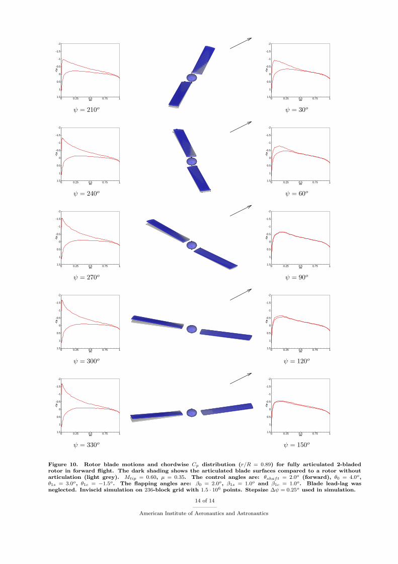
This test case involves the lifting forward flight of a fully articulated 2-bladed rotor. The rotor bladesare untapered, non-twisted with an aspect ratio of 6 and have a symmetric NACA0012 profile. For thiscase, Mtip = 0.60 and µ = 0.35. The control angles are: θshaft = 2.0o (forward), θ0 = 4.0o, θ1s = 3.0o,θ1c = −1.5o. The flapping angles are: β0 = 2.0o, β1s = 1.0o and β1c = 1.0o. Blade lead-lag was neglected.Inviscid simulation on 236-block grid with 1.5 · 106 points. Figure 9 shows the integrated blade loads fromthe 4th revolution of the simulation. The non-dimensional aerodynamic blade pitching moment and non-dimensional aerodynamic moment about the flapping hinge are shown for both blades as a function of therotor azimuth. The pitching moment curve shows the characteristic nose-up (positive) moment at the rearof the rotor disk.24–27 As the blade moves through the advancing side (i.e. 0o < ψ < 180o) the pitchingmoment shows a drastic change to a nose-down moment beyond the ψ = 90o position (where the largestblade normal velocity occurs). The moment about the flapping hinge corresponds qualitatively with theintegrated blade normal force. It can be seen that the maximum of the normal force occurs well beyond theψ = 90o position. This variation of the blade loadings is typical of helicopter rotors in (high-speed) forwardflight.24–27 Figure 10 shows the rotor blades relative to a rotor without periodic blade motions. The coningof the rotor and the flapping motions are apparent, as is the cyclic pitch. For a radial station at 89% rotorradius the chordwise Cp distribution is shown, based on the local blade normal Mach number. It is apparentthat the rotor carries the loads mainly at the front and aft of the rotor disk. The cyclic pitch clearly reduces

7 of 14


the load on the advancing side of the rotor disk. The high blade pitch on the retreating side leads to largevalues of Cp on that side of the rotor disk.

V. Summary and future work

The present framework for rotorcraft CFD is capable of routine simulations of helicopter rotors in hover.The simulation of a realistic helicopter rotor in forward flight, i.e. including the blade pitching, flappingand lead-lag motions, is tractable, but remains demanding. A CFD framework has been presented andvalidated which allows the efficient and accurate computation of helicopter rotor flows. Key ingredients are:i) the full Navier-Stokes equations which permit for non-linear, unsteady aerodynamic phenomena to becaptured, ii) the hover formulation which can simplify computations by transforming an unsteady problemto a steady-state one, iii) a novel grid-deformation strategy that allows all blade motions to be taken intoaccount separately and preserves the quality of the CFD grids and finally iv) a simple trimming algorithmthat allows computations to be performed for standard non-manoeuvering rotor conditions. Results havebeen obtained both for hovering and forward flying rotors and comparisons against experimental data areencouraging. The validation cases covered a wide range of Mach numbers and angles and for all casesthe proposed method resulted in high quality grids and efficient CPU times. This work is part of a widereffort undertaken by the authors in predicting unsteady rotor flows. Separate from validation efforts futureresearch is now directed towards the coupled rotor/ fuselage problem. The elastic deformation of the bladeshas not been considered by the present paper, however, a coupled aeroelastic analysis of the rotor is possiblewithin the present framework. In addition, the periodic nature of the flow is to be exploited for the efficientcomputation of rotor flows. These results will be reported in future papers.

Acknowledgements

The financial support of the Engineering Physical Sciences Research Council (EPSRC) and the UK Minstryof Defence (MoD) under the Joint Grant Scheme is gratefully acknowledged for this project. This workforms part of the Rotorcraft Aeromechanics Defence and BAerospace Research Partnership (DARP) fundedjointly by EPSRC, MoD, DTI, QinetiQ and Westland Helicopters.

References

1Badcock, K., Richards, B., and Woodgate, M., “Elements of Computational Fluid Dynamics on Block Structured GridsUsing Implicit Solvers,” Progress in Aerospace Sciences, Vol. 36, 2000, pp. 351–392.

2Srinivasan, G. and Baeder, J., “TURNS: A Free-wake Euler-Navier-Stokes Numerical Method for Helicopter,” AIAA jour-

nal , Vol. 31, No. 5, 1993.3Servera, G., Beaumier, P., and Costes, M., “A Weak Coupling Method between the Dynamics Code HOST and the 3D

Unsteady Euler code WAVES,” Aerospace Science and Technology, Vol. 5, 2001, pp. 397–408.4Biava, M. and Vigevano, L., “The Effect of Far-field Boundary Conditions on Tip Vortex Path Predictions in hovering,”

CEAS Aerospace Aerodynamics Research Conference, Cambridge, 10-13 June, 2002.5Boelens, O., van der Ven, H., Oskam, B., and Hassan, A., “Boundary conforming discontinuous Galerkin finite element

approach for rotorcraft simulations,” Journal of Aircraft , Vol. 39, No. 5, 2002, pp. 776–785.6Pomin, H. and Wagner, S., “Navier-Stokes Analysis of Helicopter Rotor Aerodynamics in Hover and Forward Flight,”

J. Aircraft , Vol. 39, No. 5, 2002, pp. 813–821.7Pomin, H. and Wagner, S., “Aeroelastic Analysis of Helicopter Rotor Blades on Deformable Chimera Grids,” J. Aircraft ,

Vol. 41, No. 3, 2004, pp. 577–584.8Potsdam, M., Yeo, W., and Johnson, W., “Rotor Airloads Prediction Using Loose Aerodynamic/Structural Coupling,”

American Helicopter Society 60th Annual Forum, Baltimore, MD, June 7-10, 2004.9Park, Y. and Kwon, O., “Simulation of unsteady rotor flow field using unstructured adaptive sliding meshes,” J. American

Helicopter Society, Vol. 49, No. 4, 2004, pp. 391–400.10Van der Ven, H. and Boelens, O., “A framework for aeroealistic simulations of trimmed rotor systems in forward flight,”

European Rotorcraft Forum, Marseille, September 14-16, 2004.11Conlisk, A., “Modern helicopter aerodynamics,” Annual Review of Fluid Mechanics, Vol. 29, 1997, pp. 515–567.12Bramwell, A., Helicopter Dynamics, Edward Arnold, London, 1st ed., 1976.13Seddon, J., Basic Helicopter Aerodynamics, BSP Professional books, Oxford, 1st ed., 1990.14Newman, S., The foundations of helicopter flight , Edward Arnold, London, 1st ed., 1994.15Chen, C., McCroskey, W., and Obayashi, S., “Numerical Solutions of Forward-Flight Rotor Flow Using an Upwind

Method,” J. Aircraft , Vol. 28, No. 6, 1991, pp. 374–380.16Osher, S. and Chakravarthy, S., “Upwind schemes and boundary conditions with applications to Euler equations in

general geometries,” J. Computational Physics, Vol. 50, 1983, pp. 447–481.17Jameson, A., “Time dependent calculations using multigrid, with applications to unsteady flows past airfoils and wings,”

AIAA Paper 91-1596, 1991.18Axelsson, O., Iterative Solution Methods, Cambridge University Press, Cambridge, 1994.19Steijl, R., Barakos, G., and Badcock, K., “A Framework for CFD Analysis of Helicopter Rotors in Hover and Forward

Flight,” submitted to Int. J. Num. Meth. Fluids, 2005.

8 of 14


20Schultz, K., Splettstosser, W., Junker, B., Wagner, W., and Arnaud, G. e. a., “A Parametric Windtunnel Test onRotorcraft Aerodynamics and Aeroacoustics (Helishape) - Test Procedures and Representative Results,” Aeronautical Journal ,Vol. 101, 1997, pp. 143–154.

21Caradonna, F. and Tung, C., “Experimental and analytical studies of a model helicopter rotor in hover,” Tech. Rep.TM-81232, NASA, 1981.

22Philippe, J.-J. and Chattot, J.-J., “Experimental and theoretical studies on helicopter blade tips at ONERA,” SixthEuropean Rotorcraft and Powered Lift Aircraft Forum, Bristol, September 16-19, 1980.

23Tauber, M., Chang, I., Caughey, D., and Philippe, J., “Comparison of Calculated and Measured Pressures on Straight-and Swept-Tip Model Rotor Blades,” Tech. Rep. TM-85872, NASA, 1983.

24Maier, T. and Bousman, W., “An Examination of the Aerodynamic Moment on Rotor Blade Tips Using Flight Test Dataand Analysis,” Tech. Rep. TM-104006, NASA, 1993.

25Kufeld, R., Balough, D., Cross, J., Studebaker, K., and Jennison, C., “Flight Testing the UH-60A Airloads Aircraft.”American Helicopter Society 50th Annual Forum, Washington D.C., May 11-13, 1994.

26Coleman, C. and Bousman, W., “Aerodynamic Limitations of the UH-60A Rotor,” Tech. Rep. TM-110396, NASA, 1996.27Datta, A. and Chopra, I., “Validation of structural and aerodynamic modeling using UH-60A flight test data.” J. American

Helicopter Society, Vol. 49, No. 3, 2004, pp. 271–287.

x

blade 1

blade 2

blade 3

blade 4

ω = ψz

y

ψ = 0

ψ = 90

ψ = 270

.

ψ = 180

o

o

o

o

x

y

z = z1

y

x

1

1

1

x1

z 1

y = y2z

x2

2

x 2

y2

y

x

3

3

z = z3 2

y3

z

x = x4 3

3y

z44

Rotate

FlappingLead−lag

Pitchθ

β

ψ

δ

Figure 1. Frame of reference for forward-flight simulations and rotor blade motions: rotor rotation, bladeflapping, blade lead-lag, blade pitch.

9 of 14


(a) (b)

Figure 2. (a) Detail of the multi-block topology (140 blocks) used for one blade of the 4-bladed 7A rotor.20

Around the blade, a C-H topology is used with ’extruded’ blocks towards far-field and ’hub’ surface. (b)Shaded surface forms bounding surface of grid blocks selected to move as ’rigid’ blocks with harmonic blademotion.

0.2 R0.75 R0.9 RR

OA213OA209

−4.32

−3.49−4.545

geometric twist

shaf

t

7A20

NACA0012 NACA0012

R 0.1R

shaf

t

Caradonna and Tung21

0.2 R0.75 RR

OA213OA209

−3.49−4.545

0.9 R

−4.32

0.95 R

geometric twist

shaf

t

7AD120

Figure 3. Definition of geometry of HELISHAPE 7A/7AD120 rotor blades and Caradonna and Tung21 rotorblade. For the 7A/7AD1 rotors, the non-linear geometric twist relative to the datum at 20% radius is shown.The 7AD1 planform shows the parabolic tip taper and anhedral. The Caradonna and Tung is untapered anduntwisted.

10 of 14


x/c

Cp

0 0.25 0.5 0.75 1

-1.5

-1

-0.5

0

0.5

1

1.5

r/R = 0.68 (upper): periodicr/R = 0.68 (lower): periodicExp: r/R = 0.68 (upper)Exp: r/R = 0.68 (lower)

0o collective: r/R = 0.68

x/c

Cp

0 0.25 0.5 0.75 1

-1.5

-1

-0.5

0

0.5

1

1.5



x/c

Cp

0 0.25 0.5 0.75 1

-1.5

-1

-0.5

0

0.5

1

1.5



x/c

Cp

0 0.25 0.5 0.75 1

-2

-1.5

-1

-0.5

0

0.5

1

1.5



x/c

Cp

0 0.25 0.5 0.75 1

-2

-1.5

-1

-0.5

0

0.5

1

1.5



x/c

Cp

0 0.25 0.5 0.75 1

-2

-1.5

-1

-0.5

0

0.5

1

1.5



Figure 4. Caradonna and Tung21 rotor in hover. Non-lifing case: Mtip = 0.44, 0o collective pitch. Lifting case:Mtip = 0.52, 8o collective pitch. Comparison of computed surface pressure with experimental data.

x/c

Cp

0 0.25 0.5 0.75 1

-2

-1.5

-1

-0.5

0

0.5

1

1.5

r/R = 0.48 (upper)r/R = 0.48 (lower)Exp: r/R = 0.48

7A: r/R = 0.480

x/c

Cp

0 0.25 0.5 0.75 1

-2

-1.5

-1

-0.5

0

0.5

1

1.5


7A: r/R = 0.914

x/c

Cp

0 0.25 0.5 0.75 1

-2

-1.5

-1

-0.5

0

0.5

1

1.5


7A: r/R = 0.987

x/c

Cp

0 0.25 0.5 0.75 1

-2

-1.5

-1

-0.5

0

0.5

1

1.5

r/R = 0.50: 0.6M (upper)r/R = 0.50: 0.6M (lower)r/R = 0.50: 1.3M (upper)r/R = 0.50: 1.3M (lower)Exp: r/R = 0.50

7AD1: r/R = 0.500

x/c

Cp

0 0.25 0.5 0.75 1

-2

-1.5

-1

-0.5

0

0.5

1

1.5


7AD1: r/R = 0.915

x/c

Cp

0 0.25 0.5 0.75 1

-2

-1.5

-1

-0.5

0

0.5

1

1.5


7AD1: r/R = 0.975

Figure 5. HELISHAPE 7A/7AD120 model rotors in hover, Mtip = 0.6612, 7.5o collective (at 70% rotor radius).Comparison of computed surface pressure with experimental data.

11 of 14


iteration

CT

δθ 0

,δβ 0

1000 1500 2000 2500 30000

0.0025

0.005

0.0075

0.01

-2

-1.5

-1

-0.5

0

0.5

1

1.5

2

2.5

3

target

re-trimmed

δ β0

δ θ0

cT

a) Target CT = 0.0050

iteration

CT

δθ 0

,δβ 0

1000 1500 2000 2500 30000.005

0.0075

0.01

0.0125

0.015

-2

-1.5

-1

-0.5

0

0.5

1

1.5

2

2.5

3

3.5

4

target

re-trimmed

δ β0

δ θ0

cT

b) Target CT = 0.0068

Figure 6. HELISHAPE 7A20 model rotor in hover. Trimming simulations, Mtip = 0.6612. Inviscid simulationson 140-block grid with 0.6 · 106 grid points.

t/c17%

14.5

%

shaf

t axi

s

0.37

0.80

1.0 r/R

9%

Straight blade

14.5

%

30o

1.00 r/Rshaf

t axi

s

17%

14.5

%

13.5

%

t/c9%

0.33

2

0.71

9

0.82

0

0.85

7

Swept-tip blade

Figure 7. Geometrical definition of ONERA 2-bladed model rotors.22,23

12 of 14


ψ = 60

ψ = 90

ψ = 150

ψ = 120

o

o

o

o

ψ = 30o

Straight blade

ψ = 60

ψ = 90

ψ = 150

ψ = 120

o

o

o

o

ψ = 30o

Swept-tip blade

Figure 8. Surface pressure distribution on advancing blade of non-lifting ONERA model rotor22,23 for bothblade geometries at advance ratio µ = 0.45. For the straight blade, Mtip = 0.60 (inviscid simulation on 236-blockgrid with 2.0 · 106 grid points). For the swept-tip blade, Mtip = 0.628 (inviscid simulation on 344-block grid with2.6 · 106 grid points). Stepsize ∆ψ = 0.25o used in simulations.

ψ [deg]

nond

im.b

lade

pitc

hin

gm

omen

t

0 45 90 135 180 225 270 315 360-0.15

-0.1

-0.05

0

0.05

0.1

0.15

0.2

blade 1 blade 2

ψ [deg]

non

dim

.bla

defla

ppi

ngm

omen

t

0 45 90 135 180 225 270 315 360

-14

-12

-10

-8

-6

-4

-2

0

2

4

blade 1

blade 2

Figure 9. Integrated rotor blade loading for fully articulated 2-bladed rotor in forward flight. Mtip = 0.60,µ = 0.35. The control angles are: θshaft = 2.0o (forward), θ0 = 4.0o, θ1s = 3.0o, θ1c = −1.5o. The flappingangles are: β0 = 2.0o, β1s = 1.0o and β1c = 1.0o. Blade lead-lag was neglected. Non-dimensional aerodynamicblade pitching moment and non-dimensional aerodynamic moment on flapping hinge. Inviscid simulation on236-block grid with 1.5 · 106 points. Stepsize ∆ψ = 0.25o used in simulation.

13 of 14


x/c

-Cp

0 0.25 0.5 0.75 1

-2

-1.5

-1

-0.5

0

0.5

1

1.5

ψ = 210o

x/c

-Cp

0 0.25 0.5 0.75 1

-2

-1.5

-1

-0.5

0

0.5

1

1.5

ψ = 30o

x/c

-Cp

0 0.25 0.5 0.75 1

-2

-1.5

-1

-0.5

0

0.5

1

1.5

ψ = 240o

x/c

-Cp

0 0.25 0.5 0.75 1

-2

-1.5

-1

-0.5

0

0.5

1

1.5

ψ = 60o

x/c

-Cp

0 0.25 0.5 0.75 1

-2

-1.5

-1

-0.5

0

0.5

1

1.5

ψ = 270o

x/c-C

p0 0.25 0.5 0.75 1

-2

-1.5

-1

-0.5

0

0.5

1

1.5

ψ = 90o

x/c

-Cp

0 0.25 0.5 0.75 1

-2

-1.5

-1

-0.5

0

0.5

1

1.5

ψ = 300o

x/c

-Cp

0 0.25 0.5 0.75 1

-2

-1.5

-1

-0.5

0

0.5

1

1.5

ψ = 120o

x/c

-Cp

0 0.25 0.5 0.75 1

-2

-1.5

-1

-0.5

0

0.5

1

1.5

ψ = 330o

x/c

-Cp

0 0.25 0.5 0.75 1

-2

-1.5

-1

-0.5

0

0.5

1

1.5

ψ = 150o

Figure 10. Rotor blade motions and chordwise Cp distribution (r/R = 0.89) for fully articulated 2-bladedrotor in forward flight. The dark shading shows the articulated blade surfaces compared to a rotor withoutarticulation (light grey). Mtip = 0.60, µ = 0.35. The control angles are: θshaft = 2.0o (forward), θ0 = 4.0o,θ1s = 3.0o, θ1c = −1.5o. The flapping angles are: β0 = 2.0o, β1s = 1.0o and β1c = 1.0o. Blade lead-lag wasneglected. Inviscid simulation on 236-block grid with 1.5 · 106 points. Stepsize ∆ψ = 0.25o used in simulation.

14 of 14


a cfd framework for analysis of helicopter · pdf filea cfd framework for analysis of...

Documents