a candidate young massive planet in orbit around the

A CANDIDATE YOUNG MASSIVE PLANET IN ORBIT AROUND THE CLASSICAL T TAURI STAR CI TAU*

Christopher M. Johns-Krull1,9, Jacob N. McLane

2,3, L. Prato

2,9, Christopher J. Crockett

4,9, Daniel T. Jaffe

5,

Patrick M. Hartigan1, Charles A. Beichman

6,7, Naved I. Mahmud

1, Wei Chen

1, B. A. Skiff

2, P. Wilson Cauley

1,8,

Joshua A. Jones1, and G. N. Mace

5

1 Department of Physics and Astronomy, Rice University, MS-108, 6100 Main Street, Houston, TX 77005, USA2 Lowell Observatory, 1400 West Mars Hill Road, Flagstaff, AZ 86001, USA; [email protected], [email protected] Department of Physics & Astronomy, Northern Arizona University, S San Francisco Street, Flagstaff, AZ 86011, USA

4 Science News, 1719 N Street NW, Washington, DC 20036, USA5 Department of Astronomy, University of Texas, R. L. Moore Hall, Austin, TX 78712, USA

6 Jet Propulsion Laboratory, California Institute of Technology, 4800 Oak Grove Drive, Pasadena, CA 91109, USA7 NASA Exoplanet Science Institute (NExScI), California Institute of Technology, 770 S. Wilson Avenue, Pasadena, CA 91125, USA

8 Department of Astronomy, Wesleyan University, 45 Wyllys Avenue, Middletown, CT 06459, USAReceived 2015 October 1; revised 2016 May 7; accepted 2016 May 16; published 2016 August 1

ABSTRACT

The ∼2Myr old classical T Tauri star CI Tau shows periodic variability in its radial velocity (RV) variationsmeasured at infrared (IR) and optical wavelengths. We find that these observations are consistent with a massiveplanet in a ∼9 day period orbit. These results are based on 71 IR RV measurements of this system obtained overfive years, and on 26 optical RV measurements obtained over nine years. CI Tau was also observedphotometrically in the optical on 34 nights over ∼one month in 2012. The optical RV data alone are inadequate toidentify an orbital period, likely the result of star spot and activity-induced noise for this relatively small data set.The infrared RV measurements reveal significant periodicity at ∼9 days. In addition, the full set of optical and IRRV measurements taken together phase coherently and with equal amplitudes to the ∼9 day period. Periodic RVsignals can in principle be produced by cool spots, hotspots, and reflection of the stellar spectrum off the inner disk,in addition to resulting from a planetary companion. We have considered each of these and find the planethypothesis most consistent with the data. The RV amplitude yields an M isin of ∼8.1MJup; in conjunction with a1.3 mm continuum emission measurement of the circumstellar disk inclination from the literature, we find a planetmass of ∼11.3MJup, assuming alignment of the planetary orbit with the disk.

Key words: planets and satellites: formation – stars: individual (CI Tau) – stars: low-mass – stars: pre-mainsequence – star spots – techniques: radial velocities

1. INTRODUCTION

Exoplanetary systems are common and literally come in allsizes and configurations. These span a parameter space thatencompasses more apparently stable arrangements than everimagined for multi-planet systems, from the hyper-compactKOI-500 (Ragozzine et al. 2012) to the decades- and centuries-long orbits of the HR 8799 planets (Marois et al. 2010), inmotion around a vast range of host stars. Intriguingly, however,although exoplanetary systems are found around main-sequence stars, post-main-sequence giants, brown dwarfs(Chauvin et al. 2004), intermediate age stars (Quinnet al. 2014), and even pulsars (Wolszczan & Frail 1992), todate there are no confirmed radial velocity (RV) detections ofexoplanets caught in the act of formation around very youngstars.

There are good reasons for this. Stellar systems presumablyin the process of forming planets in circumstellar orcircumbinary disks are typically located at relatively largedistances, i.e., >120 pc. The ∼10Myr TW Hya region, at50 pc, is much closer but contains only a few handfuls of youngstars, many, but not all (Bergin et al. 2013), evolved beyond theplanet-forming stage (Schneider et al. 2012). Young moving

groups near the Sun contain greater numbers of stars but areolder yet, and, given their dispersion from their molecularcloud birthplaces, are not only more challenging to age-date,but are also mostly devoid of primordial planet-forming rawmaterials (Simon et al. 2012). Tantalizingly, directly imagedplanets in these moving groups are typically associated withprocessed debris disks (e.g., Su et al. 2009; Apai et al. 2015),but the planetary bodies themselves have moved well past theformation stage. Thus it is unknown precisely when and atwhat distances from the parent star planets form, how rapidlythey migrate or are disrupted and/or ejected, and at what ageplanetary systems acquire stable configurations.The obstacles to planet surveys around newly formed stars in

the closest regions, such as Ophiuchus and Taurus, aredaunting, particularly in the case of classical T Tauri stars(CTTSs), few Myr year old solar analogues with opticallythick, actively accreting circumstellar disks. Not only are thesestars correspondingly faint, but they are also among the mostvariable classes of nearby objects (Xiao et al. 2012; Staufferet al. 2014). From relatively mild forms of variability, such asthe changes originating from spots on the surface of a rapidlyrotating star (e.g., Herbst et al. 2002), to clumpy accretionprocesses in the presence of strong magnetic fields (Gra-ham 1992; Johns-Krull et al. 1999), to extreme FU Oribehaviors and ideopathic outbursts/dimmings on the order of avisual magnitude or more detected on short timescales (e.g.,Fischer et al. 2012; Hillenbrand et al. 2013). In these

The Astrophysical Journal, 826:206 (22pp), 2016 August 1 doi:10.3847/0004-637X/826/2/206© 2016. The American Astronomical Society. All rights reserved.

* This paper includes data taken at The McDonald Observatory of TheUniversity of Texas at Austin.9 Visiting Astronomer at the Infrared Telescope Facility, which is operated bythe University of Hawaii under cooperative agreement NCC 5-538 with theNational Aeronautics and Space Administration, Office of Space Science,Planetary Astronomy Program.

1

brought to you by COREView metadata, citation and similar papers at core.ac.uk

provided by Caltech Authors

https://core.ac.uk/display/77926934?utm_source=pdf&utm_medium=banner&utm_campaign=pdf-decoration-v1

mailto:[email protected]

mailto:[email protected]

http://dx.doi.org/10.3847/0004-637X/826/2/206

http://crossmark.crossref.org/dialog/?doi=10.3847/0004-637X/826/2/206&domain=pdf&date_stamp=2016-08-01

http://crossmark.crossref.org/dialog/?doi=10.3847/0004-637X/826/2/206&domain=pdf&date_stamp=2016-08-01

environments, subtle observations of transits, direct imaging,and RV monitoring are fraught with complications.

Notwithstanding the challenges, impressive progress hasbeen made in the search for young planets, largely throughdirect imaging studies (Neuhäuser et al. 2005; Luhmanet al. 2006; Lafrenière et al. 2008; Schmidt et al. 2008; Irelandet al. 2011; Kraus & Ireland 2012; Bowler et al. 2013; Delormeet al. 2013; Kraus et al. 2014; Sallum et al. 2015). The firstputative imaged exoplanet, 2M1207b, was identified as acomoving companion to the substellar M8 dwarf 2M1207 inthe TW Hya association (Chauvin et al. 2004, 2005). The LkCa15 system, located in the younger Taurus region, was imagedusing non-redundant masking by Kraus & Ireland (2012) whonoted an unusual pattern of near- and mid-infrared (IR)emission in the inner hole of the LkCa 15 transition disk.Several years of observations of LkCa 15 have revealedapparent orbital motion (Ireland & Kraus 2014) and, morerecently, apparent accretion (Sallum et al. 2015) onto thecandidate protoplanet. Mass estimates for these objects comefrom comparing their estimated luminosity and temperaturewith theoretical evolutionary models. However, such modelsare uncertain at these young ages and the observations requiredto determine the luminosity and temperature with adequateprecision are challenging and yield considerable uncertainty inthe final mass estimate for a given object. The companion toGQ Lup (Neuhäuser et al. 2005) has mass estimates that rangefrom 1 MJUP to ∼40 MJUP (Neuhäuser et al. 2008). In additionto direct imaging of potential planetary mass companions,some suggestive results have come from transit searches. VanEyken et al. (2012) and Ciardi et al. (2015) observed transitspotentially attributable to a planetary mass object in a ∼half-day orbit around a <3Myr old T Tauri star in the Orion region,although these results have been called into question by Yuet al. (2015) and Howarth (2016).

The relative lack of confirmed planetary mass companions tovery young stars may provide clues to the planet formationprocess, or may simply be a testament to the difficulty infinding young planets. However, the transformational image ofthe HL Tau system taken in the recently commissioned long-baseline configuration with ALMA reveals numerous disk gapshighly suggestive of ongoing planet formation at a very youngage (ALMA Partnership et al. 2015). To fully understand theplanet formation and migration process, we will need toidentify newly formed planets around these young, difficulttargets. This particularly includes looking for close-in Jupiter-mass and larger companions. RV surveys have revealed theexistence of a brown dwarf desert (e.g., Marcy & Butler 2000),an unexpected paucity of close brown dwarf companions tosolar-type stars. It is not yet known if this distribution ofsecondaries is the result of the formation process itself or theresult of evolution. Armitage & Bonnell (2002) suggest thatdisks massive enough to form brown dwarf companions will beso massive that these companions inevitably interact with thedisk, migrate in, and merge with the central star. In this case,close brown dwarf companions may be detected with higherfrequency among young stars, particularly those still sur-rounded by massive disks.

In the last decade our team has undertaken an RV survey of∼140 T Tauri stars in the Taurus region to look for signaturesof RV variability indicative of young, massive planets in short-period orbits. Although we began our program at McDonaldObservatory with high-resolution spectroscopy exclusively at

optical wavelengths, we soon added high-resolution IR follow-up spectroscopy at the NASA IRTF for candidate confirmation.Visible light line bisector analysis, used to distinguish betweenthe spot and companion origins of RV variability (e.g., Huertaet al. 2008; Prato et al. 2008), is ineffective unless the v isin ofthe star is significantly greater than the spectrograph resolutionelement. Thus for a star with v isin values <10 km s−1 and aresolution R=60,000 spectrograph, we obtain at most fourresolution elements, insufficient for the line bisector analysis(Desort et al. 2007). Because the photosphere-star spot contrastis reduced in the IR, the impact of star spots on IR RVobservations is reduced by a factor of at least four in the K band(Mahmud et al. 2011). This serves as a key discriminantbetween the presence of spots or a planet, which the linebisector analysis failed to provide (Prato et al. 2008). Huélamoet al. (2008) used this approach to show that the suspectedplanet around TW Hya (Setiawan et al. 2008) was most likely afalse signal produced by spots on this rapidly rotatingyoung star.The current methodology for obtaining relatively high-

precision IR RVs requires fitting observed or synthetic templatespectra, representing the telluric spectrum, and a syntheticstellar photospheric spectrum to the observed spectrum of acandidate exoplanet host star in the 2.3 μm range. This regionof the K band is rich in both deep CO Δν=2 lines for late-type stars and in relatively deep lines of CH4 in the Earth’satmosphere. Precisions of better than 100 m s−1 have beendemonstrated by e.g., Blake et al. (2010), Figueira et al. (2010),Bean et al. (2010), Crockett et al. (2011), Bailey et al. (2012),and Davison et al. (2015) with this approach; relatively high-RV precision is possible even for remarkably active T Tauristars (Crockett et al. 2012).For the RV standard star GJ 281, Crockett et al. (2012) used

IR spectroscopy to identify an rms scatter of 66 m s−1 in RVmeasurements taken with the CSHELL spectrograph on theNASA IRTF 3 m over 48 epochs, and 30 m s−1 with theNIRSPEC spectrograph on the Keck II telescope over 9 epochs.For CI Tau, a 2Myr old, 0.80±0.02Me (Guilloteau et al.2014), CTTS with an actively accreting circumstellar disk,Crockett et al. found that the amplitude of the RV variationswas essentially the same in both the optical and K band,potentially suggestive of a planetary mass companion. Usingthe 10 optical and 14 IR measurements available at that time,Crockett et al. tentatively identified two periods in the availablesignals; however, no significance or uncertainty in thisperiodicity was identified. Since the publication of Crockettet al., we have invested considerable effort in time domainobservations of CI Tau to confirm this tentative result anddetermine the parameters of the system. The outcome of thisextended investigation is presented here. In Section 2 wedescribe our continued high-resolution spectroscopic observa-tions at both optical and IR wavelengths, as well as our opticalphotometry. Details of our light curve and RV analyses areprovided in Section 3. A discussion appears in Section 4 andwe summarize our conclusions in Section 5.

2. OBSERVATIONS AND DATA REDUCTION

The observations and data reduction are described below. Allthe reduced data used in this paper are available forindependent analysis at http://torre.rice.edu/~cmj/CITau.

2

The Astrophysical Journal, 826:206 (22pp), 2016 August 1 Johns-Krull et al.

http://torre.rice.edu/~cmj/CITau

2.1. IR

2.1.1. IRTF

Most of our IR RVs were taken with CSHELL (Tokunagaet al. 1990; Greene et al. 1993) at the 3 m NASA IRTF.CSHELL is a long-slit echelle spectrograph (1.08–5.5 μm) thatutilizes a Circular Variable Filter (CVF), allowing isolation of asingle order on a 256×256 InSb detector array. For ourobservations, the CVF was used to allow isolation of a 50Åspectral window centered at 2.298 μm (order 25). This region isfavorable for relatively precise spectroscopic analysis becauseof the presence of multiple photospheric absorption lines fromthe 2.293 μm CO ν=2–0 band head. Additionally, thepresence of multiple strong telluric lines, predominantly CH4

absorption features, allows us to use the Earth’s atmosphere asa “gas cell” and imprints a relatively stable wavelengthreference on our observations. The 0 5 slit produced anaverage FWHM of 2.6 pixels (0.5Å, 6.5 km s−1, measuredusing comparison lamp spectra), corresponding to a spectralresolving power of R∼46,000.

We obtained spectra of CI Tau on 34 nights between 2009November and 2014 March (Table 1). At the beginning of eachnight we took 20 flat fields and dark frames along with six Ar,Kr, and Xe comparison lamp exposures to create a wavelengthzero-point reference and dispersion solution. All targets wereobserved using 10″ nodded pairs, which enabled subtraction ofsky emission, dark current, and detector bias. Typicalintegration times were 600 s per nod (Crockett et al. 2011).Conditions permitting, on every night we obtained spectra ofthe RV standard GJ 281 and telluric standards with theidentical setup except for shorter exposure times.

The data reduction strategy, implemented entirely in IDL,has been reported in our earlier publications (e.g., Crockettet al. 2012) and follows that of Johns-Krull et al. (1999).Median filtering of individual dark frames produced a masterdark. A nightly normalized flat field was created by averagingthe flat-field exposures, subtracting the master dark frame, andthen dividing by the mean of the dark-subtracted master flat.Nodded pairs of target spectra were subtracted and thedifference image subsequently divided by the normalized flatfield. We estimated read noise from the standard deviation of aGaussian fit to a histogram of the pixel values in the differenceimage (∼30 e−). The curved spectral traces in the differenceimage were fit with a second-order polynomial to identify thelocation of maximum and minimum flux along the dispersiondirection. For optimal spectral extraction, each nod pair wasdivided into four equally spaced bins of 64 columns along thedispersion direction. Within each of these 64 column bins weconstructed a 10× oversampled “slit function” (i.e., thedistribution of flux in the cross-dispersion direction). A roughestimate of the spectrum was created by summing the pixels ineach column of the difference image for each nod position. Thelimits included in this sum are from the midpoint between thetwo nod positions on the detector to the edge of the area fullyilluminated by the flat lamp, typically 60–70 pixels in eachcolumn for each nod position. Each pixel in the bin was thensorted by its distance from the order center for the column thegiven pixel falls in. The flux in each pixel was divided by therough estimate of the spectrum for its appropriate column tonormalize all the pixels going into the slit function estimate.The flux in these offset ordered pixels was then median filteredwith a seven-point moving box. A flux estimate for each

Table 1CI Tau Infrared Spectroscopy

Julian RV σRVDate (km s−1) (km s−1) rK srK

CSHELL

2455156.098 −0.02 0.21 2.33 0.172455158.116 −0.33 0.20 1.84 0.122455160.107 −0.62 0.14 2.46 0.112455235.900 −0.49 0.24 1.94 0.162455236.851 −0.07 0.16 2.37 0.122455237.879 0.40 0.14 1.90 0.082455238.884 1.06 0.14 1.64 0.072455239.892 1.26 0.12 1.57 0.052455240.889 0.27 0.23 1.49 0.112455241.866 0.70 0.14 1.46 0.062455242.863 0.52 0.13 1.56 0.052456258.027 0.45 0.16 1.55 0.072456258.945 −1.02 0.18 1.62 0.092456259.117 −1.40 0.22 2.30 0.172456259.840 −0.48 0.11 1.38 0.042456260.879 −0.76 0.14 1.49 0.062456263.769 0.28 0.13 1.19 0.042456622.774 −0.61 0.08 0.00 0.012456623.785 0.14 0.10 0.13 0.012456624.859 1.01 0.11 0.77 0.032456625.881 0.88 0.19 1.11 0.022456626.911 0.16 0.40 0.97 0.102456690.895 −0.29 0.31 0.35 0.022456693.750 −0.45 0.63 1.51 0.402456696.769 0.74 0.15 0.95 0.082456697.773 0.20 0.17 0.94 0.052456698.747 0.13 0.46 0.90 0.142456699.748 0.08 0.14 0.93 0.052456701.745 −0.52 0.40 1.05 0.062456714.739 0.67 0.10 0.94 0.012456715.737 1.98 0.22 0.98 0.032456716.743 −0.03 0.23 0.98 0.072456717.741 1.22 0.34 0.86 0.062456723.740 0.75 0.33 0.51 0.01

NIRSPEC

2455251.727 −0.14 0.07 1.49 0.032455255.730 −0.86 0.05 1.64 0.032455522.880 −0.26 0.05 1.73 0.03

Phoenix

2456350.633a −1.24 0.06 0.34 0.012456351.614a −1.29 0.07 0.41 0.012456352.610a −0.42 0.06 0.40 0.012456353.607a 0.27 0.07 0.45 0.012456354.668a 0.27 0.07 0.22 0.012456605.732 −0.56 0.06 0.13 0.012456606.810 0.48 0.06 0.33 0.012456607.778 1.40 0.07 0.29 0.012456608.761 0.88 0.07 0.26 0.012456610.769 −1.41 0.06 0.26 0.012456643.930 1.32 0.07 0.00 0.012456644.875 −1.18 0.13 0.08 0.012456645.771 0.31 0.08 0.41 0.012456661.857 2.60 0.16 0.53 0.012456662.840 −2.01 0.13 0.48 0.012456663.817 −0.73 0.08 0.29 0.012456664.723 −1.01 0.07 0.48 0.012456666.708 −0.79 0.07 0.41 0.012456667.791 −0.49 0.07 0.24 0.01

IGRINS

3


oversampled pixel was then determined by taking the medianof all the pixels that fell in a given subpixel. This then formedthe oversampled master slit function. The multiple medianfilters generally remove the effects of cosmic rays anduncorrected bad pixels on the determination of the slit function.We then fit this master slit function to a three Gaussian model:a central Gaussian flanked by two satellite Gaussians. Theamplitude, center, and width of each Gaussian were fit as freeparameters using the IDL implementation of the AMOEBAnonlinear least-squares (NLLS) fitting algorithm (Nelder &Mead 1965). The resulting model was then normalized to unitarea. This algorithm produces four model slit functions, one foreach bin. However, the actual slit function is a smoothlyvarying function of column number. Therefore, to smooth outthe transitions from bin to bin, 256 column slit functions werecreated by linearly interpolating between the four bin slitfunctions.

To determine the total flux in each column of the spectrum,we calculated the scale factor that best matches the model slitfunction to the column data, per the recipe described in Horne(1986). In order to mask out spurious flux levels from cosmicrays, an iterative sigma-clipping algorithm was implemented.This algorithm starts with an estimate of the total noise fromthe measured read noise in the differenced image plus thePoisson noise from the target. We then subtracted our model fitfrom the data in each detector column and masked those pixelsfor which the residual was 3-σ greater than the estimated noise.One or two iterations were performed until the scale factorconverged, thus providing an optimal value of the spectrum inthat column that is largely immune to hot pixels, cosmic rays,and other artifacts. This algorithm also provides an estimate ofthe flux uncertainty at each location along the spectrum.

2.1.2. Keck

Three IR spectra were taken with NIRSPEC on the 10 mKeck II telescope in 2010 February and November (Table 1).NIRSPEC is a vacuum cryogenic, high-resolution, cross-dispersed, near-IR spectrograph that operates at the Nasmyth

focus. For our observations we used the N7 Filter(1.839–2.630 μm) with the echelle and cross-disperser anglesset 62°.72 and 36°.24, respectively, providing imaging of orders30 through 35 on the 1024×1024 InSb detector. The0 288×24″ slit yielded a median FWHM of 2.25 pixels(0.74Å, 9.6 km s−1, measured from lamp spectra), corresp-onding to a spectral resolving power R∼31,000.Multiple flat, dark, and comparison lamp frames of Ne, Ar,

Xe, and Kr were taken on every night of observation. Thecomparison lamp lines provided an initial wavelength zero-point and dispersion solution. All targets were observed using a10″ ABBA nod pattern, allowing for the subtraction of skyemission. Target integration times were typically on the orderof 30s with 2–3 coadds. On all three nights on which weobtained CI Tau spectra we observed the RV standard GJ 281and telluric standards; integration times were 10–20 s with 2–6coadds.The same data reduction procedure was applied as for the

CSHELL observations (Section 2.2.1) except that a fourth-orderpolynomial was used to trace the location of the spectra on thedetector instead of a second-order polynomial. Reductions werelimited to spectral order 33 (2.286–2.320 μm) because itcontains the requisite stellar CO and telluric CH4 lines andencompasses the CSHELL bandpass, which allows for moredirect comparison of the two instruments.

2.1.3. KPNO

Observations of CI Tau and GJ 281 were obtained with thePhoenix IR echelle spectrometer (Hinkle et al. 1998) duringfour separate observing runs in 2013 and 2014. Data wereobtained at the KPNO 4m Mayall telescope from 2013February 27 through 2013 March 3. All other KPNO data wereobtained at the 2.1 m telescope between 2013 November 9 and2014 January 10 (Table 1). At both telescopes the four-pixelslit was used, corresponding to 0 7×28″ at the Mayall 4 mand 1 4×56″ at the KPNO 2.1m. The grating wasconfigured to provide wavelength coverage from 2.2943 to2.3040 μm, and the K4308-order blocking filter was used toeliminate light from any overlapping orders. This setup yieldeda spectral resolution of R∼50,000 at both telescopes.Observations of each star were taken in pairs with a nod of10″ along the slit for the Mayall 4 m telescope and a nod of 20″along the slit at the KPNO 2.1 m telescope. Signal-to-noiseratios (S/N) varied significantly for the Phoenix observationsdepending on the combination of object brightness, telescopeused, and observing conditions for the observation. At theMayall 4m, typical observations on CI Tau consisted of four600 s exposures, while for GJ 281 two 600 s exposures weremost often used. At the KPNO 2.1m, eight 900 s observationswere typically made of CI Tau, while four 900 s exposures ofGJ 281 were sufficient. A total of 19 observations of CI Tauand 9 of GJ 281 were taken. In addition to stellar spectra, flat-field and dark exposures were also obtained, as well asexposures of a Th–Ar–Ne lamp in order to provide wavelengthcalibrations. All of the data were reduced using custom IDLroutines. These are essentially the same routines used to reducethe CSHELL data, with small modifications made to accountfor the differences in detector size and data formats of eachinstrument.

Table 1(Continued)

Julian RV σRVDate (km s−1) (km s−1) rK srK

2456925.895 −0.89 0.32 1.45 0.012456940.827 2.14 0.32 1.18 0.042456984.776 0.90 0.34 1.29 0.072456985.924 −0.04 0.15 0.88 0.032456986.908 0.95 0.20 0.87 0.042456987.851 −1.03 0.31 1.08 0.052456988.855 0.36 0.13 1.33 0.032456989.788 −1.07 0.13 1.56 0.012456990.813 −1.19 0.27 1.45 0.072456991.704 −1.42 0.23 1.39 0.072456992.686 0.87 0.24 1.19 0.042456993.745 0.20 0.35 1.38 0.052456996.826 0.43 0.21 1.22 0.062456997.686 −0.39 0.28 1.70 0.102457029.577 −0.77 0.54 1.03 0.07

Note.a For these nights, Phoenix was mounted on the KPNO 4 m; all other Phoenixdata were taken with the KPNO 2.1 m.

4


2.1.4. McDonald Observatory

We obtained 14 observations of CI Tau on the Harlan J.Smith 2.7 m telescope with the Immersion GRating INfraredSpectrograph (IGRINS) in 2014 November and December and2015 January (Table 1). IGRINS implements silicon immersiongratings, a fixed optical path (no cryogenic mechanisms), andvolume-phase holographic gratings to simultaneously cover theH and K bands (1.48–2.48 μm) with a resolving powerR∼45,000. The echellogram for each band is projected ontoa pair of 2048×2048 pixel Teledyne H2RG HgCdTedetectors. IGRINS’s straightforward design and high through-put make observations on the 2.7 m Harlan J. Smith Telescopeat McDonald Observatory comparable to spectrographs at 8 mfacilities, but with 5 times to 100 times the spectral grasp.Additional discussion on the design and capabilities of IGRINSappears in Park et al. (2014).

Observations with IGRINS employed standard near-IRtechniques. CI Tau was nodded between two positions,separated by 7 0, along the 1×15 arcsec slit. The IGRINSpipeline package PLP10 was developed by Dr. Jae-Joon Lee atKorea Astronomy and Space Science Institute and ProfessorSoojong Pak’s team at Kyung Hee University. The pipelinesubtracts AB pairs to remove OH emission lines and thenoptimally extracts the sources based on the methods of Horne(1986). The wavelength solution is determined first from Th–Ar lamp spectra taken at the start of each night, and thenimproved by fitting the OH lines in the two-dimensional targetspectra. The flux, wavelength, S/N, and variance of everyextracted order is output as a FITS file for the H and K bandsseparately. For our determination of CI Tau RVs we employedthe CO band-head lines redward of ∼2.295 μm.

2.2. Optical

2.2.1. Echelle Spectroscopy

CI Tau was included among the earliest subset of targetsobserved in our McDonald Observatory RV survey of ∼140stars in the Taurus region to look for evidence of young, verylow-mass companions to newly formed stars. The observa-tional setup has been described in previous papers from thiswork (Huerta et al. 2008; Prato et al. 2008; Mahmudet al. 2011; Crockett et al. 2012); we provide a brief summaryhere. Spectra were obtained with the Robert G. Tull CoudéSpectrograph (Tull et al. 1995) at the McDonald Observatory2.7 m Harlan J. Smith telescope. A total of 29 spectra wereobtained between 2004 December 28 and 2013 November 15(Table 2). A 1 2 slit yielded a spectral resolving power ofR≡λ/Δλ∼60000 for spectra covering the wavelength range3900–10000Å with small wavelength gaps between the redderorders starting at ∼5600Å. Integration times varied from 1200to 3000 s, depending on conditions, but were usually 2400 s.The average seeing was ∼2″. We took Th–Ar lamp exposuresbefore and after each spectrum for wavelength calibration;typical rms values for the dispersion solution precisionwere ∼4 m s−1.

The optical echelle spectra were reduced using a suite of IDLroutines that have been described in various references (e.g.,Valenti 1994; Hinkle et al. 2000). These routines form the basisof the REDUCE IDL echelle reduction package (Piskunov &Valenti 2002). The raw spectra were bias subtracted using the

overscan region and flat fielded using the spectrum of aninternal continuum lamp. Optimal extraction to remove cosmicrays and improve signal was used for all the spectra. Thewavelength solution was determined by fitting a two-dimen-sional polynomial to nλ as function of pixel and order number,n, for approximately 1800 extracted thorium lines observedfrom the internal lamp assembly. The final wavelength solutionused for each observation was the average of solutions fromTh–Ar lamp exposures taken before and after each stellarexposure.

2.2.2. Photometry

The photometry was obtained with the Lowell 0.7 m f/8reflector in robotic mode. It has a permanently mounted CCDcamera that provides a 15′×15′ field at an image scale of0 9 pixel−1. The CI Tau field was targeted on fourteen nightsbetween 2012 November 7 and December 11 UT. We obtainedtwo three- minute exposures in the V filter at each visit, withseveral visits each night yielding 189 data points (Table 3). Theimages were reduced via ordinary aperture photometry with thecommercial photometry package Canopus (version 10.4.0.6).The four comparison stars were found to be constant over theobservation interval. V magnitudes for these standard stars wereadopted from ASAS-3 (Pojmanski 1997) and APASS (Henden& Munari 2014) to adjust the data approximately to standard Vmagnitudes. Because of the emission-line nature of the CI Tauspectrum, there will inevitably be a small zero-point shiftdependent on the color of the comparison stars and thepassband of the filter +CCD system. Our mean magnitude nearV=13.0 is nevertheless similar to the longer-term ASAS-3value (V = 13.04), the TASS MkIV series (V = 13.1; Droegeet al. 2006), and APASS with sparser observations (V = 12.94).

3. ANALYSIS

3.1. IR RVs

All near-IR K-band observations were processed in essen-tially the same way using procedures described by Crockettet al. (2011). The RVs were determined using a spectralmodeling technique in which template spectra for the stellarspectrum and the telluric spectrum are combined to model eachof the observed spectra of CI Tau. We interpolated over a gridof NextGen models (Hauschildt et al. 1999) to produce asynthetic stellar atmosphere tailored to the Teff, log g, andmetallicity assumed for CI Tau. We then used SYNTHMAG(Piskunov 1999) to create a template stellar spectrum with thismodel atmosphere using an atomic line list from Kupka et al.(2000) and a CO line list from Goorvitch (1994). For thetelluric spectral template, we used the NOAO telluricabsorption spectrum of Livingston & Wallace (1991). Thetelluric absorption features in the K band provide an absolutewavelength and instrumental profile reference, similar inconcept to the iodine gas cell technique used in high-precisionoptical RV exoplanet surveys (Butler et al. 1996).We fit our observed spectra with the templates by fitting a

number of free parameters including a velocity shift and apower-law scaling factor for both the stellar and tellurictemplate. The stellar rotational and instrumental broadening arealso free parameters, as is a second-order continuum normal-ization, and a second-order wavelength dispersion. The modelspectrum is fit to each observed spectrum using the Levenberg–Marquardt method (Bevington & Robinson 1992) to optimize10 Currently available at: https://github.com/igrins/plp.

5


https://github.com/igrins/plp

the parameters of the model. The wavelength shift of the stellartemplate relative to the telluric template is then the measuredRV of the star, which we then correct for the motion of thebarycenter. We used a Monte Carlo technique to estimate theerrors in the model parameters. For each observation, wegenerated 100 simulated observations based on the measurednoise in the spectrum and refit the model to each of thesimulated observations. The standard deviation of the 100results for each parameter, and in particular the RV, was takenas the statistical uncertainty for that observation.

For the case of the Phoenix and IGRINS spectra where onlythe one final observed spectrum for each night is produced bythe reduction (see Sections 2.1.3 and 2.1.4), the aboveprocedure gives the final RV and associated uncertainty. Inthe case of CSHELL and NIRSPEC data, we perform the aboveRV analysis on each nod position in each exposure separately.The final, nightly RV was then determined by calculating theaverage of the individual nod RVs, weighted by theiruncertainties. The final uncertainty in the nightly RV wascomputed by taking the weighted standard deviation of the nodRVs and dividing by the square root of the number of nods.

The above procedure gives only an estimate of the statisticaluncertainty in each RV measurement based on the S/N in eachspectrum. We have previously assessed the long-term systema-tic uncertainties in our observations by routinely observingstars known to have stable RVs (i.e., <50 m s−1; Prato

et al. 2008; Mahmud et al. 2011; Crockett et al. 2012). ForCSHELL we have determined that the long-term stability inthis technique is 66 m s−1 and for NIRSPEC we havedetermined this long-term uncertainty to be 30 m s−1 (Crockettet al. 2012). In the case of Phoenix, we have a total of nineobservations of our RV standard GJ 281, and the standarddeviation of our RV measurements for this star is 62 m s−1,

which we take as the systematic uncertainty for our Phoenixobservations. This value is very similar to, but slightly betterthan, what we get for CSHELL. The slight improvement maybe the result of the fact that Phoenix has a somewhat higherresolution and about twice the wavelength coverage ofCSHELL. We have only four observations of GJ 281 withIGRINS, which is similar in resolution to CSHELL but coversa wider wavelength range in the region of interest. The standarddeviation of these observations is 52 m s−1; however, given thesmall number of observations, we assign a more conservativesystematic uncertainty to our IGRINS measurements of75 m s−1. We then add these systematic uncertainties inquadrature with the statistical uncertainty from each night’sobservation to obtain a final RV uncertainty for eachobservation. Our measured RVs and uncertainties for CI Taufor each IR spectrograph are presented in Table 1.All of our K-band RV measurements were calculated with

respect to the same reference: the telluric spectrum. Therefore,we combine the measurements from all instruments together

Table 2CI Tau Optical Spectroscopy

Julian RV σRV Ca II RV σCa II He I RV σHe I

Date (km s−1) (km s−1) (km s−1) (km s−1) (km s−1) (km s−1) r σr

2453367.805 −0.46 0.22 19.21 0.46 22.79 0.93 0.09 0.012453696.899 −0.03 0.26 17.66 0.24 21.82 0.60 0.12 0.012453770.777 1.05 0.25 18.43 0.40 25.19 0.94 0.66 0.022454141.782 L L 16.72 0.40 25.38 0.70 L L2454424.950 0.12 0.23 17.49 0.37 15.85 1.22 0.54 0.012455159.848 −0.71 0.21 17.89 0.60 19.47 1.51 0.31 0.022455160.819 0.59 0.14 17.53 0.53 19.67 0.61 0.79 0.022455161.787 0.96 0.20 15.44a 0.31 20.26 0.64 0.94 0.022455162.834 −0.72 0.22 17.74 0.41 21.06 1.10 1.02 0.032455163.908 −1.32 0.28 18.84 0.35 22.10 1.00 0.75 0.022455164.998 −1.75 0.26 15.43b 0.55 23.43 3.05 0.57 0.032456251.697 −0.44 0.28 18.44 0.34 21.42 0.72 0.53 0.022456252.678 −1.24 0.38 16.00 0.48 22.24 1.01 0.33 0.022456253.844 −0.68 0.24 17.23 0.51 19.79 1.08 0.27 0.012456254.680 −0.10 0.17 17.90 0.20 21.14 0.81 0.07 0.012456255.703 −0.06 0.18 17.65 0.39 22.85 0.80 0.10 0.012456256.669 −0.40 0.18 17.61 0.38 26.37 0.99 0.51 0.012456257.669 L L 18.57 0.23 25.68 2.17 L L2456257.905 L L 19.88 0.55 18.70 1.62 L L2456605.692 0.22 0.35 18.35 0.26 20.12 0.66 0.03 0.012456605.906 −0.06 0.35 19.48 0.29 21.90 0.63 0.00c 0.002456606.680 0.76 0.40 17.00 0.33 20.45 0.57 0.17 0.012456606.927 0.45 0.34 18.54 0.31 21.73 0.47 0.18 0.012456607.678 1.86 0.50 16.88 0.25 21.81 0.52 0.59 0.022456607.871 1.04 0.55 18.43 0.33 22.54 0.48 0.37 0.012456608.694 1.15 0.66 15.46 0.98 18.41 1.99 0.69 0.042456608.743 0.63 0.52 17.92 0.30 22.22 0.64 0.68 0.022456608.949 0.61 0.53 17.46b 0.32 21.88 0.66 0.60 0.022456611.659 −1.54 0.56 16.86 0.32 20.09 1.04 0.19 0.01

Notes.a Strong inverse P-Cygni absorption affecting Ca II profile. The Ca II RV is likely biased to a lower value.b Weaker inverse P-Cygni absorption affecting Ca II profile. The Ca II RV is possibly biased to a lower value.c Spectrum used as reference for relative veiling measurements. Veling is 0.0 by definition.

6


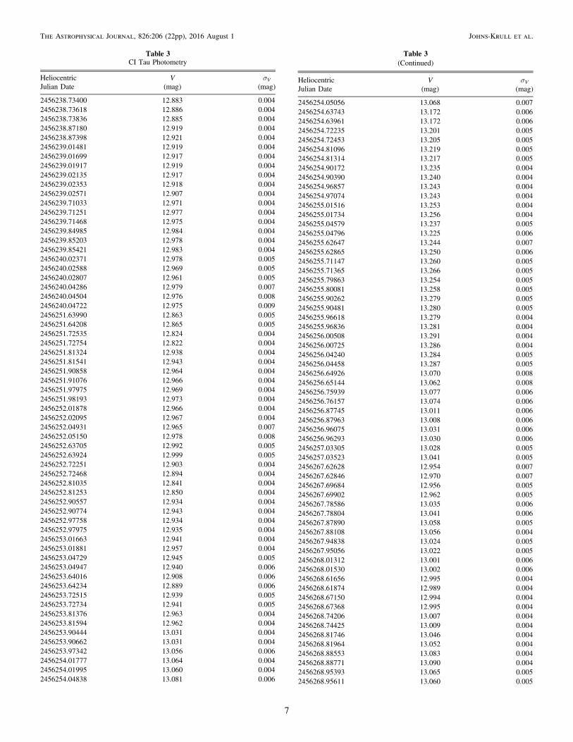
Table 3CI Tau Photometry

Heliocentric V σVJulian Date (mag) (mag)

2456238.73400 12.883 0.0042456238.73618 12.886 0.0042456238.73836 12.885 0.0042456238.87180 12.919 0.0042456238.87398 12.921 0.0042456239.01481 12.919 0.0042456239.01699 12.917 0.0042456239.01917 12.919 0.0042456239.02135 12.917 0.0042456239.02353 12.918 0.0042456239.02571 12.907 0.0042456239.71033 12.971 0.0042456239.71251 12.977 0.0042456239.71468 12.975 0.0042456239.84985 12.984 0.0042456239.85203 12.978 0.0042456239.85421 12.983 0.0042456240.02371 12.978 0.0052456240.02588 12.969 0.0052456240.02807 12.961 0.0052456240.04286 12.979 0.0072456240.04504 12.976 0.0082456240.04722 12.975 0.0092456251.63990 12.863 0.0052456251.64208 12.865 0.0052456251.72535 12.824 0.0042456251.72754 12.822 0.0042456251.81324 12.938 0.0042456251.81541 12.943 0.0042456251.90858 12.964 0.0042456251.91076 12.966 0.0042456251.97975 12.969 0.0042456251.98193 12.973 0.0042456252.01878 12.966 0.0042456252.02095 12.967 0.0042456252.04931 12.965 0.0072456252.05150 12.978 0.0082456252.63705 12.992 0.0052456252.63924 12.999 0.0052456252.72251 12.903 0.0042456252.72468 12.894 0.0042456252.81035 12.841 0.0042456252.81253 12.850 0.0042456252.90557 12.934 0.0042456252.90774 12.943 0.0042456252.97758 12.934 0.0042456252.97975 12.935 0.0042456253.01663 12.941 0.0042456253.01881 12.957 0.0042456253.04729 12.945 0.0052456253.04947 12.940 0.0062456253.64016 12.908 0.0062456253.64234 12.889 0.0062456253.72515 12.939 0.0052456253.72734 12.941 0.0052456253.81376 12.963 0.0042456253.81594 12.962 0.0042456253.90444 13.031 0.0042456253.90662 13.031 0.0042456253.97342 13.056 0.0062456254.01777 13.064 0.0042456254.01995 13.060 0.0042456254.04838 13.081 0.006

Table 3(Continued)


2456254.05056 13.068 0.0072456254.63743 13.172 0.0062456254.63961 13.172 0.0062456254.72235 13.201 0.0052456254.72453 13.205 0.0052456254.81096 13.219 0.0052456254.81314 13.217 0.0052456254.90172 13.235 0.0042456254.90390 13.240 0.0042456254.96857 13.243 0.0042456254.97074 13.243 0.0042456255.01516 13.253 0.0042456255.01734 13.256 0.0042456255.04579 13.237 0.0052456255.04796 13.225 0.0062456255.62647 13.244 0.0072456255.62865 13.250 0.0062456255.71147 13.260 0.0052456255.71365 13.266 0.0052456255.79863 13.254 0.0052456255.80081 13.258 0.0052456255.90262 13.279 0.0052456255.90481 13.280 0.0052456255.96618 13.279 0.0042456255.96836 13.281 0.0042456256.00508 13.291 0.0042456256.00725 13.286 0.0042456256.04240 13.284 0.0052456256.04458 13.287 0.0052456256.64926 13.070 0.0082456256.65144 13.062 0.0082456256.75939 13.077 0.0062456256.76157 13.074 0.0062456256.87745 13.011 0.0062456256.87963 13.008 0.0062456256.96075 13.031 0.0062456256.96293 13.030 0.0062456257.03305 13.028 0.0052456257.03523 13.041 0.0052456267.62628 12.954 0.0072456267.62846 12.970 0.0072456267.69684 12.956 0.0052456267.69902 12.962 0.0052456267.78586 13.035 0.0062456267.78804 13.041 0.0062456267.87890 13.058 0.0052456267.88108 13.056 0.0042456267.94838 13.024 0.0052456267.95056 13.022 0.0052456268.01312 13.001 0.0062456268.01530 13.002 0.0062456268.61656 12.995 0.0042456268.61874 12.989 0.0042456268.67150 12.994 0.0042456268.67368 12.995 0.0042456268.74206 13.007 0.0042456268.74425 13.009 0.0042456268.81746 13.046 0.0042456268.81964 13.052 0.0042456268.88553 13.083 0.0042456268.88771 13.090 0.0042456268.95393 13.065 0.0052456268.95611 13.060 0.005

7


and analyze them as one group with no zero-point adjustments.For the plots and the values in Table 1, we have subtracted themean of all the IR RV measurements from the reported values.We then used the Lomb–Scargle periodogram technique(Horne & Baliunas 1986) to search for periodicity in the IRRV measurements. Given the relatively large RV uncertaintieswe obtain, our data are primarily sensitive to Jupiter-mass orlarger companions in relatively tight orbits. Therefore, ourinitial periodogram search was in the range of 2–20 days (thelower bound on the period set by the Nyquist frequency sinceour observations are usually taken 1 day apart or longer). Thepower spectrum is shown in Figure 1, where a strong peak isapparent at 8.99 days. We also searched the peridogrambetween 20 and 100 days for completeness; however, nostrong peaks appear in this range (the periodogram peak in thisrange has a value of 5.8 with a false alarm probability of 0.22).We estimated the false alarm probability in the power spectrumpeak of Figure 1 using a bootstrap method where we randomlyreordered our RV measurements to create new data setsobserved with the same temporal sampling as our observations,ensuring a consistent variance for each data set. We thencomputed the power spectrum of each data set over the same2–20 day period range as done for the original data andrepeated this process 10,000 times. In doing so, we found thatthe false alarm probability for the peak seen at 8.99 day in theIR data is 6×10−4. When we fit the RV data with a Keplerianorbit (below) and subtract this fit from the data, the 8.99 daypeak and the nearby peak at ∼9.2 day vanish from the powerspectrum, indicating that there is only one potentially periodicsignal present near this period.Interpreting the periodic RV variation seen in the IR spectra

of CI Tau as orbital motion resulting from a low-masscompanion, we performed a Keplerian fit to the velocityvariations. In the orbit fitting, we keep as fixed the orbitalperiod as determined from the power spectrum analysis andtreat as free parameters the center-of-mass velocity of thesystem, the eccentricity, the velocity amplitude for CI Tau, thelongitude of periastron, and the phase of periastron passage.We use the NLLS technique of Marquardt (Bevington &Robinson 1992) to find the best-fit parameters for the orbit

Table 3(Continued)


2456269.01889 13.036 0.0062456269.02107 13.021 0.0062456269.58786 13.040 0.0042456269.59004 13.036 0.0042456269.66539 13.045 0.0042456269.66757 13.049 0.0042456269.74140 13.004 0.0042456269.74358 13.000 0.0042456269.82240 13.024 0.0042456269.82457 13.018 0.0042456269.85479 13.019 0.0042456269.85697 13.016 0.0042456269.93296 13.012 0.0042456269.93514 13.014 0.0042456269.99843 13.019 0.0052456270.00061 13.013 0.0052456270.58799 13.084 0.0052456270.59017 13.093 0.0052456270.65912 13.112 0.0042456270.66130 13.113 0.0042456270.72622 13.098 0.0042456270.72840 13.100 0.0042456270.79856 13.080 0.0042456270.80074 13.084 0.0042456270.82714 13.092 0.0042456270.82932 13.099 0.0042456270.89863 13.100 0.0042456270.90082 13.097 0.0042456270.96193 13.096 0.0052456271.58812 13.131 0.0052456271.59029 13.120 0.0052456271.65918 13.100 0.0052456271.66136 13.105 0.0052456271.72620 13.110 0.0042456271.72838 13.111 0.0042456271.80053 13.079 0.0042456271.80271 13.079 0.0042456271.83071 13.108 0.0042456271.83289 13.105 0.0042456271.89573 13.090 0.0042456271.89791 13.089 0.0042456271.95901 13.106 0.0052456271.96119 13.096 0.0052456272.58097 12.915 0.0052456272.58315 12.911 0.0042456272.63205 12.934 0.0042456272.63423 12.929 0.0042456272.68054 12.883 0.0042456272.68272 12.880 0.0042456272.74247 12.865 0.0042456272.74465 12.870 0.0042456272.79122 12.904 0.0042456272.79340 12.911 0.0042456272.83942 12.932 0.0042456272.84160 12.924 0.0042456272.84863 12.923 0.0042456272.85081 12.931 0.0042456272.89251 13.003 0.0042456272.89469 12.993 0.0042456272.93692 12.984 0.0042456272.93910 12.991 0.0042456272.98148 12.991 0.0042456272.98366 12.996 0.004

Figure 1. Power spectrum for the CI Tau IR spectroscopy based on multipleobservations at different telescopes between 2009 November and 2014November. The strongest peak appears with a nine-day period; the false alarmprobability, calculated for these irregularly sampled data with a Monte Carlosimulation (see the text), is 0.001.

8


(Table 4, column for IR only fit). While we used the peak in thepower spectrum as our initial guess for the period, wedetermined the more accurate period, reported in Table 4, thatgives a χ2 minimum for the orbital fit by densely samplingperiods near the periodogram peak period and fitting a parabolato the resulting χ2 values. The observed IR RVs for CI Tau,phased to this 8.9965 day period, along with the orbital fit areshown in Figure 2; there is considerable scatter around the fit(rms of 0.694 km s−1), which we believe to be astrophysical inorigin. We discuss the potential causes of this in Section 4.Uncertainties in the orbital fit parameters are derived by MonteCarlo simulation of the data: for 1000 simulations we constructfake RV data using the RV fit and applying Gaussian randomnoise with a standard deviation equal to that in the residualsfrom the fit of Figure 2. We then analyze these model datausing the same procedure outlined above for the actualobservations. In doing so, we keep the data uncertainties equalto the values reported in Table 1 for the purpose of the orbitfitting. The resulting uncertainties in the orbital parameters,reported as the standard deviation of the derived properties,appear in Table 4, and the distributions of the derived periods,eccentricities, and Mp sin i values are shown in Figure 3. Theinclination-dependent planetary mass of 8.81±1.71MJup wasderived assuming a stellar mass of 0.80±0.02Me for CI Tau(Guilloteau et al. 2014). The uncertainty of the planet’s massincorporates this uncertainty in the stellar mass. Guilloteauet al. determined a circumstellar disk inclination for CI Tau of45°.7±1°.1; assuming that the planet and the disk are coplanar,we find an absolute mass for CI Tau b of 12.31±2.39MJup.

3.2. Optical RVs

We followed the approach of Huerta et al. (2008) andMahmud et al. (2011) and determined optical RVs using across-correlation analysis of nine orders in the echelle spectra.Each order contains ∼100Å, and the nine orders span thewavelength range 5600–6700Å. Orders were chosen foranalysis based on high S/N, a lack of stellar emission lines,and a lack of strong telluric absorption lines present in theorder. We used the mean of the RV measurements from themultiple echelle orders as the final RV value, while thestandard deviation of the mean is assumed to be the internalstatistical uncertainty in the RV measurement. We used the CITau observation with the highest S/N (JD 2455160.819) as thetemplate for the cross-correlation analysis. Three of theobserved optical echelle spectra were not suitable for RVdeterminations owing either to contamination by a weak solarspectrum due to observations made through moderate cloudrelatively close to the moon, or to relatively low S/Ns in thecontinuum and/or large veiling values, which resulted in weakphotospheric lines and very large RV uncertainties; however,these observations remain useful for the emission-line analysis.

The RVs for these data are not reported in Table 2. Themeasured velocities were then corrected for the motion of thebarycenter and the mean RV of the optical measurements wassubtracted from all the values as we are only interested inrelative velocity variations in this study. These final optical RVmeasurements are presented in Table 2. As discussed inprevious studies from this series (e.g., Huerta et al. 2008; Pratoet al. 2008; Mahmud et al. 2011; Crockett et al. 2012), we haveobserved several RV standards known to be stable at a level ofa few m s−1 to assess the long-term stability of ourmeasurement technique. We find that our observations of thesestars show an RV standard deviation of ∼140 m s−1 for opticalwavelengths, which we take as the intrinsic uncertainty in ourmethod. We add this in quadrature to the internal uncertaintiesdetermined above to get a final optical RV measurementuncertainty, also reported in Table 2.In Section 4 we discuss the possibility that the RV variations

recorded for CI Tau result from an accretion hotspot. Thishypothesis can potentially be tested by examining thevariations in the veiling on CI Tau, and by examining thebehavior of the narrow component (NC) of emission lines suchas He I5876Å and the Ca II IR triplet (IRT). Veling in CTTSsis the apparent filling in or weakening of photosphericabsorption lines caused by a featureless continuum, believedto result from the shock that forms when accreting disk materialimpacts the stellar surface (e.g., Hartigan et al. 1989). In thisstudy we are only interested in the variations in the veiling, sowe measure a veiling, r, relative to the observation of CI Tauwith the strongest absorption lines. An accurate measure ofveiling on spectra with moderate S/N such as these is aided bycombining information from as many lines as possible. Onesuch method of doing this is to use the least-squaresdeconvolution (LSD) technique introduced by Donati et al.(1997). This technique assumes that the observed spectrum isthe convolution of a single intrinsic photospheric line profileconvolved with a series of delta functions whose location andamplitude give the wavelength and intrinsic depth of each linein the spectrum. Using a constant line list, the LSD techniquecan be used to deconvolve the spectrum to obtain the intrinsicphotospheric profile of each observation. If the lines in a givenspectrum all get weaker because of an increase in veiling, therecovered intrinsic profile will also get weaker. As a result, we

Table 4CI Tau Orbital Properties and Inferred Mass of CI Tau b

Using IR Using IR andParameter RVs Optical RVs

P (days) 8.9965±0.0327 8.9891±0.0202K (km s−1) 1.084±0.250 0.950±0.207e 0.40±0.16 0.28±0.16M isinp (MJup) 8.81±1.71 8.08±1.53

Fit rms (km s−1) 0.694 0.728

Figure 2. RVs for CI Tau based on all IR spectroscopy and phased to a periodof 8.9965 days. The average RV has been subtracted from the data. Points arecolor coded to indicate the instrument used in the observations (Table 1)

9


can compare the recovered LSD profiles from each observationand measure a very accurate relative veiling using theobservation with the strongest LSD profile as the referencespectrum. For the measurements here, we used the LSD code ofChen & Johns-Krull (2013) and a custom line list made usingthe VALD database (Kupka et al. 2000). The final line listcontains a total of 1944 lines spanning the wavelength range5350–8940Å. The majority of the lines are found in the5350–6500Å range. We used the observation from JD2456605.906 as the reference spectrum, with veiling r = 0.0by definition; all other values of veiling reported in Table 2 arerelative to this observation.

The He I5876Å and Ca II emission lines of many CTTSsappear to be made up of an NC sitting on top of a broadcomponent (BC) of the line (e.g., Batalha et al. 1996; Alencar& Basri 2000; Beristain et al. 2001). Here, we are interested inthe RV of the NC of the line. In order to isolate just this

component, we follow the example of several earlierinvestigators (Johns & Basri 1995; Alencar & Basri 2000;Sicilia-Aguilar et al. 2015) and fit each observed emission linewith multiple Gaussians. In our spectra, the only IRT linepresent is the 8662Å line so we fit this and the He I line. Giventhe higher S/N and complexity of the former, we required fourGaussian components to properly fit the Ca II line while weneeded just two Gaussian components to fit the He I line. Foreach spectrum we averaged the wavelength solution from theTh–Ar lamp spectra taken immediately before and after eachstellar spectrum. The wavelength of the NC fit was thentranslated into an RV and the motion of the barycenter wasremoved. We estimate the uncertainty in the RV by performinga Monte Carlo analysis on the fit, adding in normallydistributed random noise at a level given by the S/N in eachobservation for the line in question. A total of 100 Monte Carlotrials were performed for each line fit and the standard

Figure 3. Distribution of recovered orbital properties based on the Monte Carlo simulation of the IR-only RV data. The top panel gives the recovered period, themiddle panel gives the inferred planetary mass, and the bottom panel give the orbital eccentricity.

10


deviation of the resulting RV values was taken as theuncertainty. To this, we added in quadrature the 140 m s−1

systematic uncertainty identified above for the photosphericRV analysis. The NC RV and its uncertainty for both theHe I5876Å and Ca II8662Å lines are reported in Table 2.

CI Tau was identified as a potential host of a several Jupiter-mass planetary companion by Crockett et al. (2012) because ofits significant optical RV variations and IR (K band) RVvariations of similar amplitude; however, these results werebased on a relatively small number of data points (10 opticaland 14 IR). We now have 26 optical RV data points. Wecomputed a power spectrum of the optical RV measurements,again using the Lomb–Scargle periodogram technique (Horne& Baliunas 1986). The strongest peak in the power spectrumoccurred at a period of ∼9.5 day with a false alarm probability(determined from a Monte Carlo analysis) of 0.017. Thesecond-strongest peak in the power spectrum is nearly as strongand occurred at a period of ∼7.2 days, also with a false alarmprobability of 0.017. These peaks are suggestive, particularlysince the 7.2 day period is very close to the period found belowfor the variability of the optical photometry (Section 3.3), andthe 9.5 day period is close to the 8.99 day period found for thevariability of the IR RV measurements above (Section 3.1).However, to independently confirm periodicity, it is generallydesirable to have a false alarm probability that is lower than the0.017 observed in the optical data. As a result, the optical dataalone do not represent as significant a detection of a periodicsignal as the IR data.

3.3. Combined IR and Optical RVs

Given the periodic signals suggestive of a giant exoplanetwith a period of ∼9 days (IR) to ∼9.5 days (optical), wecombined the optical and IR mean subtracted RV data into onetime series for analysis. We again used the Lomb–Scargleperiodogram technique to compute the power spectrum of thiscombined data set (Figure 4). The peak near 9 days has becomeeven stronger, but has shifted slightly to 8.9965 days instead of8.9891 days; however, this is well within the period uncertaintydetermined from the analysis of the IR RV data alone (Table 4).We again use a bootstrap Monte Carlo technique to estimatethe false alarm probability for this peak, this time utilizing 106

trials sampling the period range 2 to 20 days as done initiallyfor the analysis of the real data. From this simulation, weestimate a false alarm probability of 8×10−6. We alsoperformed a periodogram analysis of the data in the range 2 to100 days and find that the 8.99 day period remains the strongestpeak in the data. The Monte Carlo simulation sampling thesame 2–100 day period range to estimate the false alarmprobability again yields a value of 8×10−6.

We follow the same procedure described above to fit aKeplerian orbit to this combined data set and to estimate theuncertainties in the orbital parameters. The RV fit is shown inthe bottom panel of Figure 4, which is almost identical toFigure 2. This suggests that the optical data do show evidencefor the planetary companion, but that activity-induced RVnoise muddies the planet’s signal in the optical data to somedegree. The rms of the fit residuals to the combined IR+opticalRVs is slightly greater at 0.728 km s−1 than for the IR dataalone, again likely the result of the increased activity relatednoise in the optical RV measurements. The orbital parametersand associated uncertainties are given in Table 4 and thedistribution of the derived periods, eccentricities, and MP sin i

are shown in Figure 5. We have subtracted this RV fit from theRV data points and recomputed the power spectrum of theresiduals. The highest peak in the power spectrum occurs at aperiod of 4.75 day and has a false alarm probability of 0.07. Asan additional test to see how strongly the optical data might beaffected by (and potentially biased by) spot-induced RV noise,we subtracted the IR-only RV fit (Figure 2) from the opticalRV data and computed the power spectrum of those residuals.Again, no significant peaks were found: the strongest occurs at∼4.6 days with a false alarm probability of 0.146. This couldindicate that the activity-induced variations of CI Tau do notremain coherent over the ∼9 yr span of this data, the resultperhaps of the migration of spots (e.g., Llama et al. 2012) ortheir disappearance from one region of the stellar surface andreemergence in another over the years of observation. BecauseCI Tau is a CTTS, there are many potential sources of variationin addition to dark, cool spots.The IR data alone phase nearly as well to the 8.9891 day

period, found for the combined IR plus optical data set(Figure 4), as it does to the 8.9965 day IR-only period(Figure 2). The optical data in the bottom panel of Figure 4phases fairly well to this period, although there are a fewsignificant outliers that may represent times when spot-inducednoise was particularly problematic. We emphasize that theamplitude of the optical RV variations is the same as that of theIR RV variations to within their uncertainties. If we hold the

Figure 4. Upper panel shows the power spectrum of the combined optical andIR RV times series. The peak at ∼9 days has a false alarm probability of<10−4. The lower panel shows the IR and optical RV measurements phased to8.99 days, determined from the combined RV time series.

11


orbital period and eccentricity fixed to the values found fromthe combined fit and fit only the IR RV data points, we find avelocity amplitude of K=0.99±0.17 km s−1. If we then fitonly the optical RV points holding the period and eccentricityfixed to the same values, we find K=0.63±0.23 km s−1 (thelower significance of this fit is a combination of the fewernumber of optical observations and the additional scatterpresent in the optical RVs, which in turn prevented a definitedetection of this signal in the optical-only periodogram analysisdescribed above). Thus, the optical amplitude is found to belower than that in the IR, but the difference is not statisticallysignificant.

The ratio of the optical to IR RV amplitudes is 0.64±0.26.If cool, dark spots were responsible for the RV signals in boththe optical and IR, we would expect this ratio of the optical toIR RV amplitudes to be >4 because spot noise has a higherimpact on the optical RVs (Mahmud et al. 2011). From thecombined data set, the candidate planet’s mass is

MP sin i=8.08±1.53MJup. Again assuming a stellar massof 0.80±0.02Me for CI Tau (Guilloteau et al. 2014), andusing an inclination of 45°.7±1°.1 for CI Tau b based on theinclination of the circumstellar disk (Guilloteau et al.), we getan absolute mass for CI Tau b of 11.29±2.13MJup. Thesevalues are very similar to those determined using the IR RVmeasurements alone.The eccentricity we find for CI Tau with the combined IR

and optical orbital solution, 0.28±0.16, is relatively largecompared with typical eccentricities of hot Jupiters orbitingmature stars, which are usually <0.1 (Fabrycky & Tre-maine 2007). However, the eccentricity of a few-Myr-oldobject is likely to be a property that either evolves toward zeroas the result of dynamical interactions with disk material and/or other planets, or could potentially be a property that dooms amassive planet to orbital decay and consumption by its parentstar. Alternatively, high-eccentricity giant planets may bedynamically ejected from their host system. Anecdotally, with

Figure 5. Distribution of recovered orbital properties based on the Monte Carlo simulation of the IR plus optical RV data. The top panel gives the recovered period,the middle panel gives the inferred planetary mass, and the bottom panel gives the orbital eccentricity.

12


the accumulation of larger data sets, hot exo-Jupiter eccen-tricity estimates tend to decrease. Thus, as we collect more datawe will examine the cumulative changes, if any, in eccentricityand other orbital parameters.

3.4. Optical Light Curve

We used both a Fourier-fitting routine (Harris et al. 1989)and the Lomb–Scargle method (Horne & Baliunas 1986) tolook for photometric periodicity. Both approaches yieldedsignificant power at a period of ∼7.1 days. The latter techniquegives a false alarm probability of <10−4. This value was againobtained by running 10,000 Monte Carlo simulations of thedata, sampling the observed photometry randomly over theepochs of observation. Figure 6 displays the Lomb–Scarglepower spectrum. While the power in the periodogram is quitestrong, and the data clearly show systematic variations, theperiodogram only samples this potential period in a limitedway. The photometric data were taken in 3 runs spanning atotal of 34 days. Figure 7 shows the photometry with eachobserving run color coded. The top panel shows the dataphased to the 7.1 day period found in the periodogram analysis.The bottom panel shows the data phased to the 8.99 day periodfound in the RV analysis (the figure looks the same whether wephase to 8.997 day or 8.994 day as these two periods are soclose and the length of the photometric campaign was so shortthat there is a maximum phase shift of only 0.002 between thetwo periods). Clearly the data are not strictly periodic in eitherpanel, though in the top panel (7.1 day) the data from all threeruns show a decline in brightness at approximately the samephase. For the two runs that cover the latter phases, thebrightness recovers fully at about the same phase as well, butone of these runs shows a substantially deeper minimum.Whatever is causing the decline in brightness changedmeasurably from one phase to the next, or possibly otherfactors contributed to augment the dimming. The bottom panel,phased to 8.99 days, shows no clear behavior from one phase tothe next. Because of the intrinsic jitter in the variability of thissystem, we are not able to determine a definite photometricperiod for CI Tau; however, the data do not support a period

near 9 days, and instead point to a period closer to 7 days forthis star.

3.5. Hα Analysis

All 29 optical echelle spectra of CI Tau show strong,variable Hα emission. Figure 8 shows the average Hα profileof CI Tau plotted in the stellar rest frame. This average profilehas an emission equivalent width of 69.6Å. We computed thepower spectra, again using the Lomb–Scargle method (Horne& Baliunas 1986), of the relative flux variations in each5 km s−1 velocity channel across the Hα emission line. Wefound that the velocity channel at ∼200 km s−1 (Figure 9(a))shows the strongest power, 11.0, in the periodogram analysis;this peak occurs at a period of 9.4 days. The next two strongestpeaks in this channel appear at periods of 9.0 and 9.2 days. Thesurrounding nine independent velocity channels, between 181and 227 km s−1, also show a power spectrum peak in theirrelative Hα flux variations at 9.4 days. Figures 9(b) and (c)illustrate the power spectrum from two other velocity channelsin the Hα line. Figure 9(b) shows the power spectrum of the 0velocity channel, while Figure 9(c) shows the velocity channelat −135 km s−1, which is the channel that shows the strongestfractional variation in the profile. This blueshifted velocitychannel is near the center of a variable absorption componentthat sometimes appears in the profile, indicative of a variable

Figure 6. Power spectrum for the CI Tau optical photometry based on multipleobservations per night (Table 1) over 14 nights in 2012 November andDecember. A clear peak appears with a 7.1 day period; the false alarmprobability, calculated for these irregularly sampled data with a Monte Carlosimulation (see text), is <10−4.

Figure 7. Upper panel shows the light curve showing the CI Tau V bandphotometry phased to period of 7.12 days. Uncertainties are smaller than theplot symbols. The black points are from the first observing run, red are from thesecond, and green are from the third. The bottom panel shows the same data,only this time phased to a period of 8.99 days.

13


wind flowing from CI Tau. These additional power spectraindicate the “typical” strength of the periodograms outside thestrongest one at ∼200 km s−1. The flux variations for the the200 km s−1, phased to a 9.4 day period, are shown inFigure 10(a). Again using a Monte Carlo analysis to resamplethe observed flux values in a random order while preserving theactual dates of observation, we found that the 9.4 day periodpeak in the 200 km s−1 velocity channel has a false alarmprobability less than 10−4 and any peak stronger than 9.8 has afalse alarm probability of 10−3 or less.

While the phased flux curve in Figure 10(a) shows littlescatter, the power spectrum in Figure 9(a) shows strong powerat many periods, making it unclear whether or not there is a trueperiod present. If we fit the phased flux curve in Figure 10(a)with a sine wave and subtract the fit from the data, we cancompute the power spectrum of the residuals. Doing so gives aperiodogram with a peak of only 6.3 at a period of ∼2.3 days,near the theoretical Nyquist limit for data sampled one dayapart as is typically the case for the individual runs on whichthese observations were obtained. The false alarm probabilityfor a peak this strong is 0.254. For periods longer than 3 days,the peak in the residual power spectrum occurs at ∼14.7 dayswith a power level of 5.5, corresponding to a false alarmprobability of 0.499. While the peak in the power spectrum ofthe flux variations occurs at ∼9.4 days, the next two peaks arevery close in strength and produce phased variability with littlescatter. For example, phasing to the peak at ∼9.0 days producesthe curve shown in Figure 10(b). Thus we conclude that if thereis periodic modulation in the Hα line of CI Tau, there is onlyone significant period in the 9.0–9.4 day range. These peakperiods are suggestively close to the same period as found inthe IR RV variations, possibly indicating that the source of theRV variations is also influencing the behavior of the Hα line.

4. DISCUSSION

4.1. The Role of Accretion Hotspots

Dark, cool spots can produce RV signals on a rotating starthat mimic those from a low-mass companion (e.g., Saar &Donahue 1997; Desort et al. 2007; Reiners et al. 2010). To firstorder, this results because the dark spot removes a contributionto the photospheric absorption lines at the projected RV of the

region of the rotating star where the spot is found. This leads toa distortion in the line profile, which can appear as a small RVshift. In the case of dark spots, their presence can be diagnosedon the basis of the wavelength dependence of their effect; spotsare not completely dark, and become much less so at IRwavelengths relative to the optical (e.g., Martín et al. 2006;Huélamo et al. 2008; Prato et al. 2008; Mahmud et al. 2011).This fact, and the observation that the RV amplitude of CI Tauis nearly identical in the optical and the IR, suggests that darkcool spots are not the cause of the observed RV signal in thisstar; however, there remains the possibility of hotspots.Bright accretion spots on CTTSs can in principle create the

same apparent RV signal as dark spots (e.g., Kóspál et al. 2014;Sicilia-Aguilar et al. 2015). Accretion hotspots which produceveiling on CTTSs typically have temperatures ∼10,000 K andproduce a largely featureless continuum (Hartigan et al. 1989;Basri & Batalha 1990; Hartigan et al. 1991; Valentiet al. 1993). As a result, these hotspots do not contribute tothe cool (∼4000 K) photospheric absorption lines at theprojected RV of the spot and distort the line profile shape inthe same way that a dark, cool spot would. Furthermore,because these spots are hotter than the stellar photosphere, it isexpected that they produce essentially identical line profiledistortions (and hence apparent RV signals) in the optical andthe IR. Thus, we cannot use the similarity of amplitude in theoptical and IR RV signals to rule out bright accretion spots asthe source of the observed RV signals in CI Tau. However, ifbright accretion spots are responsible for the observed RVsignals, various simple predictions may be explored to test thishypothesis. These include photometric variability produced bythe accretion spots, potential correlation between the veilingand the measured RV signals, and anti-correlation between theRV of lines formed in the hotspot with the photospheric RVsignals. We consider each of these in turn.The IR RV measurements presented here were taken over a

timespan of ∼5 yr. Including all the optical data, the timespanover which all the RV measurements we obtained is ∼10 yr.The RV measurements appear to be well phased over the 5 yrduring which the IR observations were made (Figure 2), andwith a small modification to the period (well within the perioduncertainty), the full data set shows good coherence over 10 yr(Figure 4). In order for a hotspot to produce such an RV signal,it too would have to be coherent over a similarly long timespan,and thus might be expected to show rotationally modulatedphotometric behavior. Our own photometry presented abovedoes show apparent modulation; however, while not welldetermined, the period is not consistent with the 8.99 dayperiod found in the RV signals (Figure 7). In addition to ourown observations of CI Tau, others have monitored this starphotometrically. Grankin et al. (2007) observed CI Tauphotometrically a total of 320 times between 1987 and 2003.Artemenko et al. (2012) report a period of 16.10 days based onthis data. We have downloaded this photometric database andperformed periodogram analyses on the entire data set and oneach observing season subset of the data. The highest peak werecover in the power spectrum of the entire data set is at aperiod of 16.24 days with a false alarm probability of 4.6%. Weassume this is the same signal Artemenko et al. report at aperiod of 16.10 days. We do not consider this a firm detection.Analyzing each observing season individually does not revealstronger periodicity, and in no case do we find significantperiodicity near 9 days. Percy et al. (2010) used a “self-

Figure 8. Mean Hα line profile for CI Tau. The velocity range highlighted bythe gray bar appears to show significant periodicity with a period near 9 days(see the text).

14


correlation” analysis on this same photometric data, augmentedby a few (12) additional observations and report a period of14.0 days for CI Tau. While the photometric period for CI Tauremains uncertain, the existing photometry does not suggest aperiod of 9 days for this star.

In addition to producing a photometric signal on CI Tau, if ahotspot is the cause of the observed RV variations, it is possiblethat there will be a relationship between the observed RVsignals of CI Tau and the veiling. When the hotspot is mostdirectly facing the observer (effectively in the middle of thestar), the veiling should be largest and the RV should not beaffected. As the spot moves to either limb, the veiling shoulddecrease and the RV will become either red or blueshifteddepending on which limb the spot is on. Thus, a plot of veiling

versus photospheric RV might show a parabolic relationshipwith the veiling largest at 0 relative velocity. For our opticaldata, the observed relationship between veiling and photo-spheric RV is shown in the bottom panel of Figure 11; nocorrelation was observed. We performed a correlation analysis(both linear correlation and Spearman’s and Kendal’s τ rankorder correlation) on the veiling and optical photospheric RVmeasurements and found no relationship at all between the twoquantities.The above predictions relating photometric brightness or

veiling to the photospheric RV caused by a hotspot implicitlyassume that when the accretion related continuum emissionchanges intensity, the property of the hotspot that is primarilyvarying is its projected area. If, on the other hand, accretion

Figure 9. (a) Power spectrum of the Hα velocity channel around ∼200 km s−1 showing the strongest power in the periodogram analysis. The three peaks from∼9.0–9.4 days all have a false alarm probability <10−4; however, they likely represent only one actual signal (see the text). (b) and (c): the power spectra of the Hαrelative flux variations for the velocity channels around 0 km s−1 and −135 km s−1, respectively, showing the overall weakening of the power spectrum at othervelocity channels.

15


variability causes the surface flux from the hotspot to changesubstantially on short timescales, it may be difficult to detectrotationally modulated signals from the hotspot relatedcontinuum emission. Spectroscopic studies of the veilingcontinuum emission (e.g., Valenti et al. 1993; Gullbring et al.1998; Cauley et al. 2012) find that the accretion continuum isproduced in marginally optically thick gas. These studies alsofind that the temperature of the gas producing the hotspots areall close ∼10,000 K. This suggests that the surface flux of theaccretion hotspots is very similar from star to star. Using theparmeters of the accretion emission published by Cauley et al.(2012), we find that the accretion luminosity is very wellcorrelated with the area of the star covered by the accretionspots. The studies above compare the properties of accretionspots from one CTTS to another; however, simulations ofvariable accretion onto individual CTTSs show that variationsin the area of the accretion spots are highly correlated with theinstantaneous accretion rate (e.g., Kulkarni & Romanova 2008;Romanova et al. 2008; Kurosawa & Romanova 2013). Indeed,Batalha et al. (2002) performed a variability study of the CTTSTW Hya and find that the projected area of the hotspot is wellcorrelated with the hotspot luminosity and resulting veiling.

Therefore, we suggest that the hotspot emission strength on CITau may be a good diagnostic of the projected area of thehotspot on this star as assumed in the tests described above.Another prediction of the accretion hotspot on a rotating star

hypothesis is that there should be apparent rotational modula-tion of emission lines formed in the accretion footprintsthemselves. Further, because these emission lines reveal theactual motion of the hotspot, whereas the impact of the hotspoton the photospheric absorption lines is to remove a contributionto the line profile, the modulation of the hotspot emission linesshould be 180° out of phase with the photospheric lines. Thus,plotting the emission-line RV versus the photospheric RVshould show an inverse correlation. Such behavior has beenseen in the star EX Lup by Kóspál et al. (2014) and has beenmodeled as an accretion spot by Sicilia-Aguilar et al. (2015).The lines showing this behavior are the NCs of metallicemission lines such as that from He I5876Å and the Ca II IRtriplet. It has long been expected that the NCs of these andother emission lines form in the post-shock region (e.g.,Batalha et al. 1996; Beristain et al. 2001) at the base of theaccretion footprints. As a result, the NCs of these emissionlines serve as good indicators of the behavior and location ofaccretion footprints, and they have even been used to Dopplerimage the location of accretion footprints on CTTSs (e.g.,Donati et al. 2008, 2010).We have estimated the location and size of the hotspot

required to produce the observed photospheric RV modulationusing the disk integration code utilized by Chen & Johns-Krull(2013). A single hotspot is assumed on the surface of CI Tau,and we assume a stellar inclination of 45°.7 (Guilloteau et al.2014) and a v sin i=11 km s−1 (Basri & Batalha 1990). Wefind a best fit to the observed photospheric RV measurementsfor a hotspot located at a latitude of 82° covering a maximumprojected area 46.7% on the surface of the star. Such a largeareal hotspot coverage is far greater than values typically foundon CTTSs, which are usually in the few percent range (e.g.,Valenti et al. 1993; Calvet & Gullbring 1998). However, thereis a degeneracy between the spot latitude and the size such thata hotspot covering only 10% of the stellar surface at a latitudeof 16° produces an almost equally good fit (χ2 reduced by only4%). Such a relatively small, low-latitude hotspot would showa large RV modulation (10 km s−1 peak to peak) that is 180°out of phase with the photospheric RV measurements,producing an inverse correlation between the photosphericRV measurements and RV measurements for emission linescoming from the hotspot. We looked for this behavior in theNCs of the He I5876Å and Ca II 8662Å lines.The RV signals of these two emission lines are plotted

versus the optical photospheric RV measurements in the toptwo panels of Figure 11. We performed correlation analysesusing both the linear correlation coefficient and the Spearman’sand Kendal’s τ rank order correlation coefficients. Nocorrelation was observed. The most significant correlation withthe photospheric RVs is for the RV measurements of the He I

line, but the false alarm probability is 0.58 for Kendal’s τ andhigher still for the other statistics. We also performed aperiodogram analysis on the emission-line RV measurementsand the veiling measurements, as well as phase folding these tothe 8.9965 and 8.9891 day periods. In all cases, no significantsignal was found. As a result, there is no evidence that ahotspot is producing the RV signals seen in the photosphericabsorption lines, and long-term photometric measurements do

Figure 10. (a) Phased (p = 9.4 days) Hα flux variation curve for the velocitychannel showing the strongest power, shown in the periodogram in Figure 9(a).(b) Phased Hα flux variation curve for the same velocity channel shown inFigure 9(a) but phased to p=9.0 days. The data phase well at this period also,indicating that we are not able to narrow down the true period beyond statingthat it is likely in the range 9.0–9.4 days.

16


not show the signal expected from a long-lived coherenthotspot if it were responsible for the observed RV variations inCI Tau. Thus, we suggest that it is unlikely that a hotspot isresponsible for the photospheric RV signals seen in this star.

4.2. Scattering Off an Inner Disk Wall

CI Tau is a CTTS surrounded by a circumstellar accretiondisk. The disk mass for CI Tau has been estimated by severalauthors (Andrews & Williams 2005, 2007; McClure et al.2013; Mohanty et al. 2013) with values that range from18.7MJup (Mohanty et al. 2013) to 71.3MJup (McClureet al. 2013). McClure et al. (2013) estimate that the inner diskof CI Tau is truncated at a radius of 0.12 au, which is close tothe apastron distance (0.10 au assuming e = 0.28) of thesuspected planet found in our RV analysis. The inner disk canscatter incident starlight, adding a scattered light spectrum to

the directly observed spectrum of the star. Such a scattered lightspectrum was detected in the optical for the spectroscopicbinary star KH 15D by Herbst et al. (2008). These authors findthat the reflected light from the disk is about 3% of the directspectrum in the optical near 6000Å, and that the reflectedcomponent can cause measurable effects on optical line profilesat certain phases in the binary orbit. For a single star with anazimuthally symmetric disk, this type of scattering shouldproduce a symmetric reflected light line profile centered on thestellar line, and would not therefore be expected to produce anyapparent RV shift. However, the inner walls of circumstellardisks are believed to be warped or otherwise not symmetric inmany cases, resulting in detectable photometric variability(e.g., Cody et al. 2014; Stauffer et al. 2014; McGinniset al. 2015). If there is some coherent structure at or near theinner wall of the accretion disk, it might contribute a scatteredlight component that is Doppler shifted along our line of sight

Figure 11. Top panel shows the Ca II8662 Å RV measurements vs. the photospheric RV measurements for the optical data. The middle panel shows the He I5876 ÅRV values vs. the photospheric RVs, and the bottom panel shows the optical veiling vs. the photospheric RV values. No significant correlation was found in any ofthese plots.

17


relative to the star as a result of the orbital motion of the disk.As the structure orbits the star, its velocity shift relative to thestar would change, potentially distorting the photosphericabsorption lines and creating an apparent velocity signal forthe star.

For a structure at the inner wall of the disk to be responsiblefor the observed RV signatures above, it must be located at adistance where the period is equal to 8.99 days. For the0.80Me mass of CI Tau, this corresponds to 0.079 au, wellinside the 0.12 au inner wall of the disk found by McClure et al.(2013). Looking at it another way, the orbital period at 0.12 auis 17 days, substantially longer than the period of RVvariations. In order to produce the observed RV variations,such a disk structure would need to remain stable over the nine-year span of the data collected here. Such stability is unlikelygiven the short dynamical time of the disk at this radius, unlessthe disk structure, such as a warp, is excited and maintained bysome other object or process. A massive planet inside the diskgap could excite such a disk structure. The interaction of theinner disk wall with the stellar magnetosphere, particularly ifthe magnetosphere is tilted, could also excite a long-term stabledisk warp as is believed to be the case for AA Tau for example(Bouvier et al. 2003, 2013). Such a disk warp is tied to thestellar rotation, which our photometric monitoring suggests hasa period of ∼7 days instead of 9 days. Another estimate for therotation period of CI Tau can be made using its v sin i, stellarradius, and inclination. Assuming that the inclination of the staris equal to that of the disk, we can use i=55° andR*=1.41 Re (both from McClure et al. 2013). Takingv sin i=11 km s−1 again from Basri & Batalha (1990), therotation period is estimated to be 5.3 days. This estimateshrinks somewhat to 4.6 days using the inclination of 45°.7degrees from Guilloteau et al. (2014), and i=90 gives anestimated period of 6.5 days. There are of course uncertaintiesin the stellar radius and v sin i, so these period estimates arethemselves uncertain; however, the available measurementspoint to a rotation period noticeably less than the 8.99 dayperiod of the RV variations.

While the estimates above argue that some sort of structurein the inner disk wall scattering starlight from CI Tau isprobably not responsible for the RV variations we measure, wecan look to the data for evidence one way or another. Thespectral model used to measure the K-band RVs in Section 3.1includes a term that measures the strength of the 2.29 μm K-band photospheric lines, which can vary as the result of veiling,a meaure of the continuum emission from the inner diskrelative to that from the star (e.g., Folha & Emerson 1999;Johns-Krull & Valenti 2001). If there is a coherent structure inthe inner disk responsible for scattering starlight and producingthe observed RV variations, we might expect there to be acorrelation between the K-band veiling and the measured RVs.We convert our measurements into the K-band veiling(measured at 2.29 μm as opposed to averaged over the entireband), referenced to the model spectrum used in the fittingprocess. These K-band veilings are reported in Table 1. Wephase the K-band veilings with respect to the 8.99 day RVperiod in Figure 12, but we find no apparent pattern with thephase. We also computed the periodogram of the K-bandveiling measurements, finding no significant peaks near ninedays. In particular, the false alarm probability of the highestpeak within ±5 days of 8.99 days is 0.81, with the period of thepeak being 13.6 days. Thus, our IR observations do not show

any relationship between the disk emission and the mea-sured RVs.We can also estimate the level of scattering that would be

needed to produce the observed RV signal. As mentionedabove, in order to produce periodicity at ∼9 days, the scatteringsurface in the disk would need to be at radius of ∼0.08 auwhere the Keplerian velocity is ∼96 km s−1. Using i=45°.7,this surface would vary in RV by ±68 km s−1 relative to thestar. As the lines in the scattered light spectrum move throughthe stellar spectrum, they can distort the photospheric lineprofile and appear to produce a velocity shift. We estimate thestrength of the required scattered light spectrum by asking howstrong the scattered light line profile would need to be relativeto the stellar lines in order to produce the ±1 km s−1 shift thatis observed in the RV signal (Figure 4). We first assumed thatthe scattered light spectral lines are identical to those in the star.This assumes the scattering source is essentially a point in thedisk so that the reflected stellar spectrum is not smeared invelocity space because of formation around a range in azimuthin the disk. We used the the LSD Stokes I photospheric profilescalculated for the optical spectra in Section 3.2 and added ascaled version of the same spectrum to the original profileshifted by a specified RV value. We stepped through shifts of±68 km s−1 in 0.1 km s−1 steps and used the same cross-correlation technique as in Section 3.2 to measure the resultingRV shift. We find that in order to produce a maximum linedistortion of ±1 km s−1, the scattered light spectrum needs tobe ∼17% the strength of the directly observed stellar spectrum(Figure 13). If this were indeed occuring, a feature 17% as deepas the observed profiles would be present in the spectra of CITau and would move periodically back and forth relative to themain lines by ±68 km s−1. Such a feature would be obvious inthe LSD optical profiles (Figure 13) and is not seen. If weinstead represent the scattered light spectrum as the stellarspectrum convolved with a Gaussian of FWHM = 40 km s−1 tomimic scattering from a range of disk azimuth, we find that thescattered light component must be ∼57% as strong as the stellarspectrum in order to produce the measured RV variations. Sucha strong component is not seen in the observed spectra, and thishigh level of scattering is also unphysical (e.g., Whitney &Hartmann 1992). We conclude that it is highly unlikely thatscattering off the inner disk is producing the RV variations weobserve.

Figure 12. K-band veiling vs. phase determined from the combined optical-plus-IR RV fit (Figure 4).

18


4.3. The Challenge and Necessity of FindingPlanets around CTTSs

We conclude that the best interpretation of the data presentedin this paper is that there is a ∼11–12MJUP mass planet on asomewhat eccentric ∼9 day orbit around the CTTS CI Tau. Wehave illustrated some of the unique difficulties in searching forplanets around actively accreting young stars. However, inorder to understand planet formation, it will be necessary tolook for planets in just such systems. All indications of thethousands of planets identified by the Kepler mission, as wellas the structure and likely dynamic history of our own solarsystem, point to significant evolution and migration of planets,including the gas giants (e.g., Levison et al. 2007, p. 669). Inorder to begin to document and characterize the extent of theseprocesses, and to determine the nature of planet formationitself, we are compelled to search for the first generation ofplanets around host stars with extreme and variable properties.

CTTSs undergoing active accretion present complex chal-lenges for the identification of even giant planets on short-period orbits. Some of these have been described above.Potential sources of variable photometry include changes ingeometry and extinction resulting from modifications in theline of sight across or through the circumstellar disk as itrotates. Furthermore, bright accretion footprints and episodicaccretion events, cool stellar spots, stellar flares, massivecoronal mass ejections, and stellar jet outbursts, among otherphenomena, may all contribute to a particularly high level ofactivity and thus variability. Spectral absorption line profilevariability may result from the shift in an absorption line centeras a large dark spot (or spots) is carried across the observedstellar hemisphere by the star’s own rotation. Hotspots fromaccretion or flares on the stellar surface may produce ananalogous result. Accreting hot gas, and warm dust grains inthe inner disk, may give rise to a continuum excess that veilsabsorption lines and can, in extreme cases, effectively obliteratethem. Strong variability in emission-line fluxes and line profilesresult from excitation arising in clumpy accretion flows, stellarwinds, and jets (e.g., Alencar et al. 2005). Yet it is at thistumultuous phase in a star’s lifetime during which planets musthave already formed or be in the formation process, given the

relatively short window of availability of the reservoir of rawmaterial in the primordial disk.The evidence we present for a giant planet in the CI Tau

system is demonstrated on the basis of diverse data setscollected over 10 yr at five different facilities. Over this multi-year timescale we find consistent variability in the IR RVs, aswell as evidence in the optical RV variations, for this sameperiodic signal, supporting our planetary companion interpreta-tion. Some significant scatter is obvious in the IR RVs plottedin Figures 2 and 4; we interpret this as likely the result ofastrophysical processes, such as those described above.Although working in the IR diminishes the impact of coolstar spots and stellar activity, it does not guarantee immunityfrom these phenomena, particularly in a classical T Taurisystem. Some processes, such as emission from warm grains inan inner circumstellar disk, may wield a greater impact in theIR. However, although this work is outside the scope of thiscurrent paper, we are hopeful that it will be possible tominimize these sources of interference in our RV measure-ments. For example, for stars with known rotation periods,specific observing allocations in the future can be used to tailorthe IR spectroscopic observations to take place repeatedly atthe same rotational phase of the star (e.g., Robertsonet al. 2015), thus nulling any spot signal. We can alsoexperiment with spot modeling in order to determine the degreeof interference anticipated in our IR RV measurements, andwith extracting contaminating spot signals from our spectradirectly (e.g., Llama et al. 2012; Moulds et al. 2013; Bradshaw& Hartigan 2014; Aigrain et al. 2015).The behavior of activity on young stars is not well

understood. Astronomers know that extreme cases are possible,for example unusually long-lived spots that appear to phasecoherently over many years (Stelzer et al. 2003; Mahmudet al. 2011; Bradshaw & Hartigan 2014), or spots with fillingfactors that cover most of the stellar surface (Hatzes 1995).Although T Tauri stars are all presumed to have strongmagnetic fields and corresponding activity (Johns-Krull 2007),it is not uncommon to find systems that defy characterization oftheir rotation periods on the basis of spots (e.g., Xiaoet al. 2012). CTTSs, with their many types of potential activity,are among the most difficult for the measurement of rotation,although many show variable behavior that at times reveals

Figure 13. Three representative LSD profiles from the optical spectra, showing the observations with the smallest and largest measured RV as well as the observationclosest to zero RV. The red profile shows the same profile offset by −60 km s−1 and scaled to 17% to show the strength of the scattering feature needed to produce themeasured RV variations (see text). The phase (f) and RV of each observation is given.

19


periodic light curve behavior (Herbst et al. 2002). CI Tauappears to fit into this category. The peculiar activity thatdistinguishes CTTSs is embodied by the Hα line and itsvariations. This line is a strong accretion diagnostic, and theHα variability of CI Tau is intriguing. The red side of theprofile shows potentially periodic variability that phases wellwith the orbital period of the likely planetary companion(Figure 8). The exact cause of this variability is not clear,however. The Hα luminosity of accreting roughly planetarymass objects may be as high as 10% that of the central star(e.g., Zhou et al. 2014), so it is possible this variability resultsfrom the RV motion of Hα emission associated with the planetitself. In that case, one would expect similar periodicity at allvelocities sampled by the planetary orbit, as long as they arestrong enough relative to the line profile variations from the staritself. It is also possible that this apparent periodicity in the Hαline is caused by the planet modulating the accretion of diskmaterial onto the star, similar to that seen in close, eccentricbinary CTTSs like DQ Tau (e.g., Basri et al. 1997). In eithercase, the Hα variability of CI Tau deserves furtherinvestigation.

The definitive characterization of a massive planet in the CITau system will require continued monitoring for an RV signalin the IR consistent with the orbital parameters identified todate and corroborating results from optical RV observations,modulo potentially variable cool spot noise. A firm detection ofthe photometric rotation period with a period different from theRV period would also help substantiate the existence of aplanet orbiting CI Tau. Verification of our result mustnecessarily rely for now on these ground-based techniques asthe candidate CI Tau planet will not be astrometricallydetectable by the GAIA mission, for example (Sozzettiet al. 2014).

5. SUMMARY

We have identified a ∼9 day period in the K-band RVvariations of the CTTS CI Tau. The best interpretation of thesedata is that a massive planet is in orbit around this young starlocated in the Taurus star-forming region. This identification isbased on high-resolution IR spectroscopy supported by high-resolution optical spectroscopy and optical photometry, allcollected over a 10 yr total timespan. For the ∼5 yr of our IRobservations of CI Tau, from 2009 to 2014, the RVs extractedfrom the spectroscopy phase to a period of ∼9 days. While notsufficient to independently confirm the ∼9 day period, the fullset of optical RVs also phase reasonably well to the ∼9 day RVperiod observed in the IR spectroscopy. While it is expectedthat the optical RV measurements experience a greater impactfrom cool star spots than the IR RVs, the amplitude of theoptical RV variations is very similar to those observed in theIR, indicating that noise from cool spots does not obliterate theplanetary signal. We also investigate the possibility that theobserved photospheric RV variations on this CTTS result froman accretion hotspot or from scattering off the inner wall of theaccretion disk. These scenarios gives rise to a few potentiallytestable predictions which are not supported by the datacollected here or by other investigators. Therefore, we find thatthe best interpretation of the observations presented here is thatthe RV variability of CI Tau results from reflex motion inducedby a ∼11–12MJup planet. Furthermore, we find that the flux inthe +200 km s−1 region of CI Tau’s Hα emission line varieswith an apparent periodicity of ∼9 days, suggestive of detection

of accretion onto the planet at a particular orbital phase. Whilethe period of ∼9 days is strongly detected in our data, the largelevel of astrophysical noise means that some of the orbitalparameters (e.g., the eccentricity) are not well determined. Afirmer detection of the rotation period of the star is also needed.As a result, more observations of CI Tau are critical to confirmthis important result, as well as additional observations todetect giant planets around other young stars. An excess in theyoung hot Jupiter population may indicate the prevalence ofdestructive mechanisms, which result in the relative paucity ofmassive, short-period planets around main-sequence stars,∼1% (e.g., Wright et al. 2012). A massive planet in a ∼9 dayperiod orbit around a 2Myr old star places strong constraintson planet formation and migration timescales. It is key to ourunderstanding of exoplanet evolution to determine the extent towhich such systems are common.

We thank the IRTF TOs Dave Griep, Bill Golisch, and EricVolquardsen and SAs John Rayner, Mike Connelly, and BobbyBus, the Keck Observatory OAs Cynthia Wilburn and HeatherHershley and SAs Scott Dahm and Greg Wirth, KPNO staffDave Summers, Di Harmer, and Dick Joyce, and Dave Doss ofMcDonald Observatory for their exceptional observing supportover the many years of this program. L.P. is grateful to PeterBodenheimer, Joe Llama, Evgenya Shkolnik, and Ben Zucker-man for insightful discussions. Partial support for this researchwas provided by the SIM Young Planets Key Project and byNASA Origins grants 05-SSO05-86 and 07-SSO07-86 to L.P.Additional support for this work was provided by the NSFthrough grant AST-1212122 made to Rice University. We aregrateful to the Arizona Space Grant consortium for support ofJ.N.M.’s participation in this work. We wish to thank ananonymous referee for many helpful comments that improvedthe manuscript. This work made use of the SIMBAD referencedatabase, the NASA Astrophysics Data System, and the dataproducts from the Two Micron All Sky Survey, which is a jointproject of the University of Massachusetts and the InfraredProcessing and Analysis Center/California Institute of Tech-nology, funded by the National Aeronautics and SpaceAdministration and the National Science Foundation. Thiswork made use of the Immersion Grating InfraredSpectrograph (IGRINS) that was developed under a collabora-tion between the University of Texas at Austin and the KoreaAstronomy and Space Science Institute (KASI) with thefinancial support of the U.S. National Science Foundationunder grant AST-1229522, of the University of Texas atAustin, and of the Korean GMT Project of KASI. Some datapresented herein were obtained at the W. M. Keck Observatory,which is operated as a scientific partnership among theCalifornia Institute of Technology, the University of California,and the National Aeronautics and Space Administration. Theobservatory was made possible by the generous financialsupport of the W. M. Keck Foundation. The authors recognizeand acknowledge the significant cultural role that the summit ofMauna Kea plays within the indigenous Hawaiian community.We are grateful for the opportunity to conduct observationsfrom this special mountain.

REFERENCES

Aigrain, S., Llama, J., Ceillier, T., et al. 2015, MNRAS, 450, 3211Alencar, S. H. P., & Basri, G. 2000, AJ, 119, 1881Alencar, S. H. P., Basri, G., Hartmann, L., & Calvet, N. 2005, A&A, 440, 595

20


http://dx.doi.org/10.1093/mnras/stv853

http://adsabs.harvard.edu/abs/2015MNRAS.450.3211A

http://dx.doi.org/10.1086/301300

http://adsabs.harvard.edu/abs/2000AJ....119.1881A

http://dx.doi.org/10.1051/0004-6361:20053315

http://adsabs.harvard.edu/abs/2005A&A...440..595A

ALMA Partnership, Brogan, C. L., Pérerz, L. M., et al. 2015, ApJL, 808, 3Andrews, S. M., & Williams, J. P. 2005, ApJ, 631, 1134Andrews, S. M., & Williams, J. P. 2007, ApJ, 659, 705Apai, D., Schneider, G., Grady, C. A., et al. 2015, ApJ, 800, 136Armitage, P. J., & Bonnell, I. A. 2002, MNRAS, 330, L11Artemenko, S. A., Grankin, K. N., & Petrov, P. P. 2012, AstL, 38, 783Bailey, J. I., III, White, R. J., Blake, C. H., et al. 2012, ApJ, 749, 16Basri, G., & Batalha, C. 1990, ApJ, 363, 654Basri, G., Johns-Krull, C. M., & Mathieu, R. D. 1997, AJ, 114, 781Batalha, C., Batalha, N. M., Alencar, S. H. P., Lopes, D. F., & Duarte, E. S.

2002, ApJ, 580, 343Batalha, C. C., Stout-Batalha, N. M., Basri, G., & Terra, M. A. O. 1996, ApJS,

103, 211Bean, J. L., Seifahrt, A., Hartman, H., et al. 2010, ApJ, 713, 410Bergin, E. A., Cleeves, L. I., Gorti, U., et al. 2013, Natur, 493, 644Beristain, G., Edwards, S., & Kwan, J. 2001, ApJ, 551, 1037Bevington, P. R., & Robinson, D. K. 1992, Data Reduction and Error Analysis

for the Physical Sciences (2nd ed.; New York: McGraw-Hill)Blake, C. H., Charbonneau, D., & White, R. J. 2010, ApJ, 723, 684Bouvier, J., Grankin, K., Ellerbroek, L. E., Bouy, H., & Barrado, D. 2013,

A&A, 557, A77Bouvier, J., Grankin, K. N., Alencar, S. H. P., et al. 2003, A&A, 409, 169Bowler, B. P., Liu, M. C., Shkolnik, E. L., & Dupuy, T. J. 2013, ApJ, 774, 55Bradshaw, S. J., & Hartigan, P. 2014, ApJ, 795, 79Butler, R. P., Marcy, G. W., Williams, E., et al. 1996, PASP, 108, 500Calvet, N., & Gullbring, E. 1998, ApJ, 509, 802Cauley, P. W., Johns-Krull, C. M., Hamilton, C. M., & Lockhart, K. 2012,

ApJ, 756, 68Chauvin, G., Lagrange, A.-M., Dumas, C., et al. 2004, A&A, 425, L29Chauvin, G., Lagrange, A.-M., Dumas, C., et al. 2005, A&A, 438, L25Chen, W., & Johns-Krull, C. M. 2013, ApJ, 776, 113Ciardi, D. R., van Eyken, J. C., Barnes, J. W., et al. 2015, ApJ, 809, 42Cody, A. M., Stauffer, J., Baglin, A., et al. 2014, AJ, 147, 82Crockett, C. J., Mahmud, N. I., Prato, L., et al. 2011, ApJ, 735, 78Crockett, C. J., Mahmud, N. I., Prato, L., et al. 2012, ApJ, 761, 164Davison, C. L., White, R. J., Henry, T. J., et al. 2015, AJ, 149, 106Delorme, P., Gagné, J., Girard, J. H., et al. 2013, A&A, 553, L5Desort, M., Lagrange, A.-M., Galland, F., Udry, S., & Mayor, M. 2007, A&A,

473, 983Donati, J.-F., Jardine, M. M., Gregory, S. G., et al. 2008, MNRAS, 386, 1234Donati, J.-F., Semel, M., Carter, B. D., Rees, D. E., & Collier Cameron, A.

1997, MNRAS, 291, 658Donati, J.-F., Skelly, M. B., Bouvier, J., et al. 2010, MNRAS, 409, 1347Droege, T. F., Richmond, M. W., Sallman, M. P., & Creager, R. P. 2006,

PASP, 118, 1666Fabrycky, D., & Tremaine, S. 2007, ApJ, 669, 1298Figueira, P., Pepe, F., Lovis, C., & Mayor, M. 2010, A&A, 515, A106Fischer, W. J., Megeath, S. T., Tobin, J. J., et al. 2012, ApJ, 756, 99Folha, D. F. M., & Emerson, J. P. 1999, A&A, 352, 517Goorvitch, D. 1994, ApJS, 95, 535Graham, J. A. 1992, PASP, 104, 479Grankin, K. N., Melnikov, S. Y., Bouvier, J., Herbst, W., & Shevchenko, V. S.

2007, A&A, 461, 183Greene, T. P., Tokunaga, A. T., Toomey, D. W., & Carr, J. B. 1993, Proc.

SPIE, 1946, 313Guilloteau, S., Simon, M., Piétu, V., et al. 2014, A&A, 567, A117Gullbring, E., Hartmann, L., Briceño, C., & Calvet, N. 1998, ApJ, 492, 323Harris, A. W., Young, J. W., Bowell, E., et al. 1989, Icar, 77, 171Hartigan, P., Hartmann, L., Kenyon, S., Hewett, R., & Stauffer, J. 1989, ApJS,

70, 899Hartigan, P., Kenyon, S. J., Hartmann, L., et al. 1991, ApJ, 382, 617Hatzes, A. P. 1995, ApJ, 451, 784Hauschildt, P. H., Allard, F., & Baron, E. 1999, ApJ, 512, 377Henden, A., & Munari, U. 2014, CoSka, 43, 518Herbst, W., Bailer-Jones, C. A. L., Mundt, R., Meisenheimer, K., &

Wackermann, R. 2002, A&A, 396, 513Herbst, W., Hamilton, C. M., Leduc, K., et al. 2008, Natur, 452, 194Hillenbrand, L. A., Miller, A. A., Covey, K. R., et al. 2013, AJ, 145, 59Hinkle, K., Wallace, L., Valenti, J., & Harmer, D. 2000, Visible and Near

Infrared Atlas of the Arcturus Spectrum 3727–9300 A, ed. K. Hinkle et al.(San Francisco, CA: ASP)

Hinkle, K. H., Cuberly, R. W., Gaughan, N. A., et al. 1998, Proc. SPIE,3354, 810

Horne, J. H., & Baliunas, S. L. 1986, ApJ, 302, 757Horne, K. 1986, PASP, 98, 609Howarth, I. D. 2016, MNRAS, 457, 3769

Huélamo, N., Figueira, P., Bonfils, X., et al. 2008, A&A, 489, L9Huerta, M., Johns-Krull, C. M., Prato, L., Hartigan, P., & Jaffe, D. T. 2008,

ApJ, 678, 472Ireland, M. J., Kraus, A., Martinache, F., Law, N., & Hillenbrand, L. A. 2011,

ApJ, 726, 113Ireland, M. J., & Kraus, A. L. 2014, in IAU Symp. 299, Exploring the

Formation and Evolution of Planetary Systems, ed. M. Booth,B. C. Matthews, & J. R. Graham (Cambridge: Cambridge Univ. Press), 199

Johns, C. M., & Basri, G. 1995, ApJ, 449, 341Johns-Krull, C. M. 2007, ApJ, 664, 975Johns-Krull, C. M., & Valenti, J. A. 2001, ApJ, 561, 1060Johns-Krull, C. M., Valenti, J. A., Hatzes, A. P., & Kanaan, A. 1999, ApJL,

510, L41Kóspál, Á, Mohler-Fischer, M., Sicilia-Aguilar, A., et al. 2014, A&A,

561, A61Kraus, A. L., & Ireland, M. J. 2012, ApJ, 745, 5Kraus, A. L., Ireland, M. J., Cieza, L. A., et al. 2014, ApJ, 781, 20Kulkarni, A. K., & Romanova, M. M. 2008, MNRAS, 386, 673Kupka, F. G., Ryabchikova, T. A., Piskunov, N. E., Stempels, H. C., &

Weiss, W. W. 2000, BaltA, 9, 590Kurosawa, R., & Romanova, M. M. 2013, MNRAS, 431, 2673Lafrenière, D., Jayawardhana, R., & van Kerkwijk, M. H. 2008, ApJL,

689, L153Levison, H. F., Morbidelli, A., Gomes, R., & Backman, D. 2007, in Protostars

and Planets V, ed. B. Reipurth, D. Jewitt, & K. Keil (Tucson, AZ: Univ. ofArizona Press), 669

Livingston, W., & Wallace, L. 1991, NSO Tech. Rep. #91-001 (Tucson, AZ:National Solar Observatory, National Optical Astronomy Observatory)

Llama, J., Jardine, M., Mackay, D. H., & Fares, R. 2012, MNRAS, 422,L72

Luhman, K. L., Wilson, J. C., Brandner, W., et al. 2006, ApJ, 649, 894Mahmud, N. I., Crockett, C. J., Johns-Krull, C. M., et al. 2011, ApJ, 736, 123Marcy, G. W., & Butler, R. P. 2000, PASP, 112, 137Marois, C., Zuckerman, B., Konopacky, Q. M., Macintosh, B., & Barman, T.

2010, Natur, 468, 1080Martín, E. L., Guenther, E., Zapatero Osorio, M. R., Bouy, H., & Wainscoat, R.

2006, ApJL, 644, L75McClure, M. K., D’Alessio, P., Calvet, N., et al. 2013, ApJ, 775, 114McGinnis, P. T., Alencar, S. H. P., Guimarães, M. M., et al. 2015, A&A,

577, A11Mohanty, S., Greaves, J., Mortlock, D., et al. 2013, ApJ, 773, 168Moulds, V. E., Watson, C. A., Bonfils, X., Littlefair, S. P., & Simpson, E. K.

2013, MNRAS, 430, 1709Nelder, J., & Mead, R. 1965, CompJ, 7, 308Neuhäuser, R., Guenther, E. W., Wuchterl, G., et al. 2005, A&A, 435, L13Neuhäuser, R., Mugrauer, M., Seifahrt, A., et al. 2008, A&A, 484, 281Park, C., Jaffe, D. T., Yuk, I.-S., et al. 2014, Proc. SPIE, 9147, 91471DPercy, J. R., Grynko, S., Seneviratne, R., & Herbst, W. 2010, PASP, 122, 753Piskunov, N. 1999, Polarization, 243, 515Piskunov, N. E., & Valenti, J. A. 2002, A&A, 385, 1095Pojmanski, G. 1997, AcA, 47, 467Prato, L., Huerta, M., Johns-Krull, C. M., et al. 2008, ApJL, 687, L103Quinn, S. N., White, R. J., Latham, D. W., et al. 2014, ApJ, 787, 27Ragozzine, D. & Kepler Team 2012, BAAS, 44, 200.04Reiners, A., Bean, J. L., Huber, K. F., et al. 2010, ApJ, 710, 432Robertson, P., Roy, A., & Mahadevan, S. 2015, ApJL, 805, L22Romanova, M. M., Kulkarni, A. K., & Lovelace, R. V. E. 2008, ApJL,

673, L171Saar, S. H., & Donahue, R. A. 1997, ApJ, 485, 319Sallum, S., Follette, K. B., Eisner, J. A., et al. 2015, Natur, 527, 342Schmidt, T. O. B., Neuhäuser, R., Seifahrt, A., et al. 2008, A&A, 491, 311Schneider, A., Melis, C., & Song, I. 2012, ApJ, 754, 39Setiawan, J., Henning, T., Launhardt, R., et al. 2008, Natur, 451, 38Sicilia-Aguilar, A., Fang, M., Roccatagliata, V., et al. 2015, A&A, 580, 82Simon, M., Schlieder, J. E., Constantin, A.-M., & Silverstein, M. 2012, ApJ,

751, 114Sozzetti, A., Giacobbe, P., Lattanzi, M. G., et al. 2014, MNRAS, 437, 497Stauffer, J., Cody, A. M., Baglin, A., et al. 2014, AJ, 147, 83Stelzer, B., Fernández, M., Costa, V. M., et al. 2003, A&A, 411, 517Su, K. Y. L., Rieke, G. H., Stapelfeldt, K. R., et al. 2009, ApJ, 705, 314Tokunaga, A. T., Toomey, D. W., Carr, J., Hall, D. N. B., & Epps, H. W. 1990,

Proc. SPIE, 1235, 131Tull, R. G., MacQueen, P. J., Sneden, C., & Lambert, D. L. 1995, PASP,

107, 251Valenti, J. A. 1994, PhD thesis, Univ. CaliforniaValenti, J. A., Basri, G., & Johns, C. M. 1993, AJ, 106, 2024

21


http://dx.doi.org/10.1088/2041-8205/808/1/L3

http://adsabs.harvard.edu/abs/2015ApJ...808L...3A

http://dx.doi.org/10.1086/432712

http://adsabs.harvard.edu/abs/2005ApJ...631.1134A

http://dx.doi.org/10.1086/511741

http://adsabs.harvard.edu/abs/2007ApJ...659..705A

http://dx.doi.org/10.1088/0004-637X/800/2/136

http://adsabs.harvard.edu/abs/2015ApJ...800..136A

http://dx.doi.org/10.1046/j.1365-8711.2002.05213.x

http://adsabs.harvard.edu/abs/2002MNRAS.330L..11A

http://dx.doi.org/10.1134/S1063773712110011

http://adsabs.harvard.edu/abs/2012AstL...38..783A

http://dx.doi.org/10.1088/0004-637X/749/1/16

http://adsabs.harvard.edu/abs/2012ApJ...749...16B

http://dx.doi.org/10.1086/169374

http://adsabs.harvard.edu/abs/1990ApJ...363..654B

http://dx.doi.org/10.1086/118510

http://adsabs.harvard.edu/abs/1997AJ....114..781B

http://dx.doi.org/10.1086/343110


http://dx.doi.org/10.1086/192275

http://adsabs.harvard.edu/abs/1996ApJS..103..211B

http://adsabs.harvard.edu/abs/1996ApJS..103..211B

http://dx.doi.org/10.1088/0004-637X/713/1/410


http://dx.doi.org/10.1038/nature11805

http://adsabs.harvard.edu/abs/2013Natur.493..644B

http://dx.doi.org/10.1086/320233

http://adsabs.harvard.edu/abs/2001ApJ...551.1037B

http://dx.doi.org/10.1088/0004-637X/723/1/684


http://dx.doi.org/10.1051/0004-6361/201321389

http://adsabs.harvard.edu/abs/2013A&A...557A..77B

http://dx.doi.org/10.1051/0004-6361:20030938

http://adsabs.harvard.edu/abs/2003A&A...409..169B

http://dx.doi.org/10.1088/0004-637X/774/1/55


http://dx.doi.org/10.1088/0004-637X/795/1/79


http://dx.doi.org/10.1086/133755

http://adsabs.harvard.edu/abs/1996PASP..108..500B

http://dx.doi.org/10.1086/306527

http://adsabs.harvard.edu/abs/1998ApJ...509..802C

http://dx.doi.org/10.1088/0004-637X/756/1/68

http://adsabs.harvard.edu/abs/2012ApJ...756...68C

http://dx.doi.org/10.1051/0004-6361:200400056

http://adsabs.harvard.edu/abs/2004A&A...425L..29C

http://dx.doi.org/10.1051/0004-6361:200500116

http://adsabs.harvard.edu/abs/2005A&A...438L..25C

http://dx.doi.org/10.1088/0004-637X/776/2/113


http://dx.doi.org/10.1088/0004-637X/809/1/42


http://dx.doi.org/10.1088/0004-6256/147/4/82

http://adsabs.harvard.edu/abs/2014AJ....147...82C

http://dx.doi.org/10.1088/0004-637X/735/2/78


http://dx.doi.org/10.1088/0004-637X/761/2/164


http://dx.doi.org/10.1088/0004-6256/149/3/106

http://adsabs.harvard.edu/abs/2015AJ....149..106D

http://dx.doi.org/10.1051/0004-6361/201321169

http://adsabs.harvard.edu/abs/2013A&A...553L...5D

http://dx.doi.org/10.1051/0004-6361:20078144

http://adsabs.harvard.edu/abs/2007A&A...473..983D

http://adsabs.harvard.edu/abs/2007A&A...473..983D

http://dx.doi.org/10.1111/j.1365-2966.2008.13111.x

http://adsabs.harvard.edu/abs/2008MNRAS.386.1234D

http://dx.doi.org/10.1093/mnras/291.4.658

http://adsabs.harvard.edu/abs/1997MNRAS.291..658D

http://dx.doi.org/10.1111/j.1365-2966.2010.17409.x

http://adsabs.harvard.edu/abs/2010MNRAS.409.1347D

http://dx.doi.org/10.1086/510197

http://adsabs.harvard.edu/abs/2006PASP..118.1666D

http://dx.doi.org/10.1086/521702

http://adsabs.harvard.edu/abs/2007ApJ...669.1298F

http://dx.doi.org/10.1051/0004-6361/201014005

http://adsabs.harvard.edu/abs/2010A&A...515A.106F

http://dx.doi.org/10.1088/0004-637X/756/1/99

http://adsabs.harvard.edu/abs/2012ApJ...756...99F

http://adsabs.harvard.edu/abs/1999A&A...352..517F

http://dx.doi.org/10.1086/192110

http://adsabs.harvard.edu/abs/1994ApJS...95..535G

http://dx.doi.org/10.1086/133021

http://adsabs.harvard.edu/abs/1992PASP..104..479G

http://dx.doi.org/10.1051/0004-6361:20065489

http://adsabs.harvard.edu/abs/2007A&A...461..183G

http://adsabs.harvard.edu/abs/1993SPIE.1946..313G

http://dx.doi.org/10.1051/0004-6361/201423765

http://adsabs.harvard.edu/abs/2014A&A...567A.117G

http://dx.doi.org/10.1086/305032

http://adsabs.harvard.edu/abs/1998ApJ...492..323G

http://dx.doi.org/10.1016/0019-1035(89)90015-8

http://adsabs.harvard.edu/abs/1989Icar...77..171H

http://dx.doi.org/10.1086/191361

http://adsabs.harvard.edu/abs/1989ApJS...70..899H

http://adsabs.harvard.edu/abs/1989ApJS...70..899H

http://dx.doi.org/10.1086/170749

http://adsabs.harvard.edu/abs/1991ApJ...382..617H

http://dx.doi.org/10.1086/176265


http://dx.doi.org/10.1086/306745


http://adsabs.harvard.edu/abs/2014CoSka..43..518H

http://dx.doi.org/10.1051/0004-6361:20021362

http://adsabs.harvard.edu/abs/2002A&A...396..513H


http://adsabs.harvard.edu/abs/2008Natur.452..194H

http://dx.doi.org/10.1088/0004-6256/145/3/59

http://adsabs.harvard.edu/abs/2013AJ....145...59H

http://adsabs.harvard.edu/abs/1998SPIE.3354..810H

http://adsabs.harvard.edu/abs/1998SPIE.3354..810H

http://dx.doi.org/10.1086/164037


http://dx.doi.org/10.1086/131801

http://adsabs.harvard.edu/abs/1986PASP...98..609H

http://dx.doi.org/10.1093/mnras/stw245

http://adsabs.harvard.edu/abs/2016MNRAS.457.3769H

http://dx.doi.org/10.1051/0004-6361:200810596

http://adsabs.harvard.edu/abs/2008A&A...489L...9H

http://dx.doi.org/10.1086/526415


http://dx.doi.org/10.1088/0004-637X/726/2/113

http://adsabs.harvard.edu/abs/2011ApJ...726..113I

http://adsabs.harvard.edu/abs/2014IAUS..299..199I

http://dx.doi.org/10.1086/176059

http://adsabs.harvard.edu/abs/1995ApJ...449..341J

http://dx.doi.org/10.1086/519017

http://adsabs.harvard.edu/abs/2007ApJ...664..975J

http://dx.doi.org/10.1086/323257

http://adsabs.harvard.edu/abs/2001ApJ...561.1060J

http://dx.doi.org/10.1086/311802

http://adsabs.harvard.edu/abs/1999ApJ...510L..41J

http://adsabs.harvard.edu/abs/1999ApJ...510L..41J

http://dx.doi.org/10.1051/0004-6361/201322428

http://adsabs.harvard.edu/abs/2014A&A...561A..61K

http://adsabs.harvard.edu/abs/2014A&A...561A..61K

http://dx.doi.org/10.1088/0004-637X/745/1/5

http://adsabs.harvard.edu/abs/2012ApJ...745....5K

http://dx.doi.org/10.1088/0004-637X/781/1/20

http://adsabs.harvard.edu/abs/2014ApJ...781...20K

http://dx.doi.org/10.1111/j.1365-2966.2008.13094.x

http://adsabs.harvard.edu/abs/2008MNRAS.386..673K

http://adsabs.harvard.edu/abs/2000BaltA...9..590K

http://dx.doi.org/10.1093/mnras/stt365

http://adsabs.harvard.edu/abs/2013MNRAS.431.2673K

http://dx.doi.org/10.1086/595870

http://adsabs.harvard.edu/abs/2008ApJ...689L.153L

http://adsabs.harvard.edu/abs/2008ApJ...689L.153L

http://adsabs.harvard.edu/abs/2007prpl.conf..669L

http://dx.doi.org/10.1111/j.1745-3933.2012.01239.x

http://adsabs.harvard.edu/abs/2012MNRAS.422L..72L

http://adsabs.harvard.edu/abs/2012MNRAS.422L..72L

http://dx.doi.org/10.1086/506517

http://adsabs.harvard.edu/abs/2006ApJ...649..894L

http://dx.doi.org/10.1088/0004-637X/736/2/123

http://adsabs.harvard.edu/abs/2011ApJ...736..123M

http://dx.doi.org/10.1086/316516

http://adsabs.harvard.edu/abs/2000PASP..112..137M


http://adsabs.harvard.edu/abs/2010Natur.468.1080M

http://dx.doi.org/10.1086/505343

http://adsabs.harvard.edu/abs/2006ApJ...644L..75M

http://dx.doi.org/10.1088/0004-637X/775/2/114


http://dx.doi.org/10.1051/0004-6361/201425475

http://adsabs.harvard.edu/abs/2015A&A...577A..11M

http://adsabs.harvard.edu/abs/2015A&A...577A..11M

http://dx.doi.org/10.1088/0004-637X/773/2/168


http://adsabs.harvard.edu/abs/2010iac..talk..225M

http://dx.doi.org/10.1051/0004-6361:200500104

http://adsabs.harvard.edu/abs/2005A&A...435L..13N

http://dx.doi.org/10.1051/0004-6361:20078493

http://adsabs.harvard.edu/abs/2008A&A...484..281N

http://dx.doi.org/10.1117/12.2056431

http://adsabs.harvard.edu/abs/2014SPIE.9147E..1DP

http://dx.doi.org/10.1086/654826

http://adsabs.harvard.edu/abs/2010PASP..122..753P

http://dx.doi.org/10.1007/978-94-015-9329-8_45

http://adsabs.harvard.edu/abs/1999ASSL..243..515P

http://dx.doi.org/10.1051/0004-6361:20020175

http://adsabs.harvard.edu/abs/2002A&A...385.1095P

http://adsabs.harvard.edu/abs/1997AcA....47..467P

http://dx.doi.org/10.1086/593201

http://adsabs.harvard.edu/abs/2008ApJ...687L.103P

http://dx.doi.org/10.1088/0004-637X/787/1/27

http://adsabs.harvard.edu/abs/2014ApJ...787...27Q

http://adsabs.harvard.edu/abs/2012DPS....4420004R

http://dx.doi.org/10.1088/0004-637X/710/1/432

http://adsabs.harvard.edu/abs/2010ApJ...710..432R

http://dx.doi.org/10.1088/2041-8205/805/2/L22

http://adsabs.harvard.edu/abs/2015ApJ...805L..22R

http://dx.doi.org/10.1086/527298

http://adsabs.harvard.edu/abs/2008ApJ...673L.171R

http://adsabs.harvard.edu/abs/2008ApJ...673L.171R

http://dx.doi.org/10.1086/304392

http://adsabs.harvard.edu/abs/1997ApJ...485..319S


http://adsabs.harvard.edu/abs/2015Natur.527..342S

http://dx.doi.org/10.1051/0004-6361:20078840

http://adsabs.harvard.edu/abs/2008A&A...491..311S

http://dx.doi.org/10.1088/0004-637X/754/1/39

http://adsabs.harvard.edu/abs/2012ApJ...754...39S


http://adsabs.harvard.edu/abs/2008Natur.451...38S

http://dx.doi.org/10.1051/0004-6361/201525970

http://adsabs.harvard.edu/abs/2015A&A...580A..82S

http://dx.doi.org/10.1088/0004-637X/751/2/114



http://dx.doi.org/10.1093/mnras/stt1899

http://adsabs.harvard.edu/abs/2014MNRAS.437..497S

http://dx.doi.org/10.1088/0004-6256/147/4/83

http://adsabs.harvard.edu/abs/2014AJ....147...83S

http://dx.doi.org/10.1051/0004-6361:20031414

http://adsabs.harvard.edu/abs/2003A&A...411..517S

http://dx.doi.org/10.1088/0004-637X/705/1/314


http://adsabs.harvard.edu/abs/1990SPIE.1235..131T

http://dx.doi.org/10.1086/133548

http://adsabs.harvard.edu/abs/1995PASP..107..251T

http://adsabs.harvard.edu/abs/1995PASP..107..251T

http://dx.doi.org/10.1086/116783

http://adsabs.harvard.edu/abs/1993AJ....106.2024V

van Eyken, J. C., Ciardi, D. R., von Braun, K., et al. 2012, ApJ, 755, 42Whitney, B. A., & Hartmann, L. 1992, ApJ, 395, 529Wolszczan, A., & Frail, D. A. 1992, Natur, 355, 145Wright, J. T., Marcy, G. W., Howard, A. W., et al. 2012, ApJ, 753, 160

Xiao, H. Y., Covey, K. R., Rebull, L., et al. 2012, ApJS, 202, 7Yu, L., Winn, J. N., Gillon, M., et al. 2015, ApJ, 812, 48Zhou, Y., Herczeg, G. J., Kraus, A. L., Metchev, S., & Cruz, K. L. 2014, ApJL,

783, L17

22


http://dx.doi.org/10.1088/0004-637X/755/1/42

http://adsabs.harvard.edu/abs/2012ApJ...755...42V

http://dx.doi.org/10.1086/171673

http://adsabs.harvard.edu/abs/1992ApJ...395..529W

http://dx.doi.org/10.1038/355145a0

http://adsabs.harvard.edu/abs/1992Natur.355..145W

http://dx.doi.org/10.1088/0004-637X/753/2/160

http://adsabs.harvard.edu/abs/2012ApJ...753..160W

http://dx.doi.org/10.1088/0067-0049/202/1/7

http://adsabs.harvard.edu/abs/2012ApJS..202....7X

http://dx.doi.org/10.1088/0004-637X/812/1/48

http://adsabs.harvard.edu/abs/2015ApJ...812...48Y

http://dx.doi.org/10.1088/2041-8205/783/1/L17

http://adsabs.harvard.edu/abs/2014ApJ...783L..17Z

http://adsabs.harvard.edu/abs/2014ApJ...783L..17Z

a candidate young massive planet in orbit around the

Documents