a calculation framework and tools to estimate freight rate
TRANSCRIPT

DEPARTMENT OF TECHNOLOGY MANAGEMENT AND ECONOMICS
DIVISION OF SERVICE MANAGEMENT AND LOGISTICS
CHALMERS UNIVERSITY OF TECHNOLOGY
Gothenburg, Sweden 2020
www.chalmers.se Report No. E2020:104
11
A calculation framework and tools to estimate freight rate and carbon emissions for road transport Master’s thesis in Supply Chain Management
Yinfan Hu
Daqi Liu (University of Gothenburg)


REPORT NO. E 2020:104
A calculation framework and tools to estimate
freight rate and carbon emissions for road
transport
A study at Volvo Group Trucks Operations
Yinfan Hu
Daqi Liu
Department of Technology Management and Economics
Division of Supply Chain Management
CHALMERS UNIVERSITY OF TECHNOLOGY
Gothenburg, Sweden 2020

A calculation framework and tools to estimate freight rate and carbon emissions for road transport
A study at Volvo Group Trucks Operations
Yinfan Hu
Daqi Liu
© Yinfan Hu, 2020.
© Daqi Liu, 2020.
Report no. E2020:104
Department of Technology Management and Economics
Chalmers University of Technology
SE-412 96 Göteborg
Sweden
Telephone + 46 (0)31-772 1000
Gothenburg, Sweden 2020

V
A calculation framework and tools to estimate freight rate and carbon emissions for
road transport
A study at Volvo Group Trucks Operations
Yinfan Hu
Daqi Liu
Department of Technology Management and Economics
Chalmers University of Technology
SUMMARY
The high-quality estimation methods for the freight rate and carbon emissions of road transport are not
only important to improve a company’s performance but also valuable to academia. This research
designed a framework embedded in a user-friendly computer tool to estimate the road freight rate and
transport carbon emissions. This tool is tested by estimating fright rates for various scenarios to meet
the business and operational demand of a case company, The Volvo Group. The framework is
designed based on the cost breakdown theory, which comprises of two sections. The first section
estimates the road freight rate, while the second section estimates the carbon emissions. Firstly, all
cost elements for both sections are identified. Each cost element is then studied and the most suitable
estimation method for each cost element is selected. Besides, considering the constraints and settings
of Volvo, specific sets of calculation methods are designed to acquire the estimated freight rate and
carbon emissions for different transport set-ups at Volvo.
In order to transform the theoretical framework into a user-friendly computer tool, two types of tools,
one using Excel spreadsheets and the other using the Excel VBA are developed for the case
company. The validation of the framework is conducted through the estimation of a set of scenarios at
the case company. The framework could demonstrate the rate structure and the carbon emissions for
the scenarios. Further, it could help the company to identify the major cost elements and prioritize
efforts in achieving cost savings. The differences between the bid prices and the estimated freight
rates are analyzed and interpreted from the aspects including imbalanced flow, relative power, and
operation-efficiency among carriers. In the case company, the imbalanced flow and different features
among carriers are proved to have more influence on the freight rate, while the relative power is not
regarded as a source of gaps.
Keywords: cost breakdown theory, cost elements, road freight rate, transport carbon emissions,
transport service purchasing, Excel VBA, estimation framework

VI

VII
Acknowledgment
We would like to thank all the people that have participated and contributed to this thesis
research.
We truly appreciate our thesis mentor Catrin Lammgård from Gothenburg University, School
of Business, Economics and Law, our thesis supervisor Lokesh Kumar Kalahasthi from
Chalmers University of Technology, and our thesis examiner Dan Andersson from Chalmers
University of Technology for their helpful guidance and input to this thesis project.
We are also sincerely grateful to our brilliant thesis mentors and wonderful colleagues from
the case company Volvo Group. Their kind support and extra efforts to us are the key to the
completion of this thesis project, especially during the Covid-19 situation when resources and
accessibility are highly limited.
Furthermore, we would like to extend our deep gratitude to the interviewees from the case
company for their time to the interviews.
Daqi Liu & Yinfan Hu
Gothenburg, Sweden
19th May 2020

VIII
Abbreviation
ADR: European Agreement concerning the International Carriage of Dangerous Goods by
Road
ARR: Annual Rate of Return
CDC: Central Distribution Center
DC: Distribution Center
DDS: Dedicated Delivery Service
FD: Footprint Design
FTL: Full Truck Load
GHG: Greenhouse Gas
GTO: (Volvo) Group Trucks Operations
LP: Logistics Purchasing
LSP: Logistics Service Provider
LTL: Less Than Truck Load
PL: Production Logistics
PLI: Price Level Index
POA: Period of Availability
RDC: Regional Distribution Center
SDC: Support Distribution Center
SML: Service Market Logistics
VBA: Visual Basic for Applications
Volvo: Volvo Group

IX
Contents SUMMARY .............................................................................................................................. V
Acknowledgment .................................................................................................................... VII
Abbreviation .......................................................................................................................... VIII
Contents .................................................................................................................................... IX
List of Figures ......................................................................................................................... XII
List of Tables ......................................................................................................................... XIV
1 Introduction ........................................................................................................................ 1
1.1 Research background ................................................................................................... 1
1.2 Objective and research questions ................................................................................. 3
1.3 Research scope ............................................................................................................. 3
1.4 Thesis outline ............................................................................................................... 4
2 Literature review ................................................................................................................ 5
2.1 Cost breakdown theory ................................................................................................. 5
2.2 Estimation of road freight cost ..................................................................................... 6
2.2.1 Cost classification ................................................................................................. 6
2.2.2 Cost elements and estimation methods ................................................................. 7
2.2.3 The cost structure of road freight transport ......................................................... 10
2.3 Other factors that influence freight rate ..................................................................... 11
2.3.1 Trade imbalance – backhaul problem ................................................................. 11
2.3.2 Stakeholder interaction ........................................................................................ 12
2.3.3 Size of carriers ..................................................................................................... 13
2.4 Carbon emissions calculation for road transport ........................................................ 14
2.5 Visual Basic for Applications .................................................................................... 15
3 Methodology .................................................................................................................... 17
3.1 Research outline ......................................................................................................... 17
3.2 The research onion model .......................................................................................... 18
3.3 Research approach ...................................................................................................... 18
3.4 Methodological choice ............................................................................................... 19
3.5 Research strategy ........................................................................................................ 20
3.6 Time horizon .............................................................................................................. 20
3.7 Data collection ............................................................................................................ 20
3.7.1 Primary data ........................................................................................................ 21
3.7.2 Secondary data .................................................................................................... 22

X
3.8 Reliability and validity ............................................................................................... 23
4 Company overview .......................................................................................................... 25
4.1 Company background and function description ......................................................... 25
4.2 Problem description .................................................................................................... 27
4.3 Road transport at Volvo ............................................................................................. 28
4.3.1 Overview of the transport network ...................................................................... 28
4.3.2 Transport set-ups at Volvo .................................................................................. 29
5 Design of calculation framework ..................................................................................... 34
5.1 Basic framework ........................................................................................................ 34
5.1.1 Design of Road freight section ............................................................................ 34
5.1.2 Design of Carbon emission section ..................................................................... 53
5.1.3 Summary of fact data .......................................................................................... 54
5.2 Calculation of Modules and set-ups ........................................................................... 55
5.2.1 The design of modules ........................................................................................ 55
5.2.2 Modules and set-ups in road freight rate section ................................................. 56
5.2.3 Modules and set-ups in road freight rate section ................................................. 62
6 Development of calculation tools ..................................................................................... 64
6.1 Calculation tool in VBA ............................................................................................. 64
6.1.1 Structure of the VBA-based tool ......................................................................... 64
6.1.2 Process flow of the VBA-based tool ................................................................... 65
6.2 Spreadsheet-based Tool .............................................................................................. 67
6.2.1 Structure of spreadsheet-based tool ..................................................................... 67
6.2.2 Process flow of the spreadsheet-based tool ......................................................... 68
6.3 Comparison and discussion ........................................................................................ 69
7 Test of framework analysis .............................................................................................. 71
7.1 Rate structure and carbon emission ............................................................................ 71
7.1.1 Full-Truck-Load .................................................................................................. 71
7.1.2 Less-Than-Truck-Load ........................................................................................ 76
7.1.3 Dedicated Delivery Service ................................................................................. 77
7.2 Comparison of current bid prices ............................................................................... 80
8 Discussion ........................................................................................................................ 83
8.1 Rate structure .............................................................................................................. 83
8.2 Gaps with bid prices ................................................................................................... 86
9 Conclusion and future recommendations ......................................................................... 89
9.1 Conclusion .................................................................................................................. 89

XI
9.2 Future research and recommendations ....................................................................... 90
References ................................................................................................................................ 92
Appendix A: Demonstration of tools ....................................................................................... 97
Appendix B: VBA Code ........................................................................................................ 101
Appendix C: Question list for the semi-structured interview ................................................ 104

XII
List of Figures
Figure 1-1 Thesis outline .................................................................................................................. 4
Figure 2-1 A structure of cost breakdown (Garrett, 2008) ............................................................... 6
Figure 2-2 Illustration of backhaul planning .................................................................................. 12
Figure 2-3 Long run average and marginal costs (Source: Cowie (2009)) .................................... 13
Figure 3-1 Research outline ........................................................................................................... 17
Figure 3-2 Research onion model (Saunders, Lewis, & Thornhill, 2009). .................................... 18
Figure 4-1 Structure of the organizational functions (within the scope of the thesis) ................... 26
Figure 4-2 Transport network for PL ............................................................................................. 28
Figure 4-3 Transport network for SML .......................................................................................... 29
Figure 4-4 FTL set-up outline ........................................................................................................ 31
Figure 4-5 LTL set-up outline ........................................................................................................ 31
Figure 4-6 DDS set-up outline ....................................................................................................... 32
Figure 4-7 Express set-up outline ................................................................................................... 33
Figure 5-1 Structure of the basic framework ................................................................................. 34
Figure 5-2 Cost elements in road freight rate section .................................................................... 35
Figure 5-3 Illustration of payment terms ........................................................................................ 50
Figure 5-4 Breakdown of carbon emissions ................................................................................... 53
Figure 5-5 Basic framework, modules, and set-ups ....................................................................... 55
Figure 5-6 FTL set-up and modules involved ................................................................................ 57
Figure 5-7 LTL set-up and modules involved ................................................................................ 57
Figure 5-8 DDS set-up and modules involved ............................................................................... 58
Figure 5-9 Relations of capacity, loads and shipment size ............................................................ 61
Figure 6-1 Structure of VBA-based tool ........................................................................................ 64
Figure 6-2 Process flowchart of the VBA-based tool .................................................................... 66
Figure 6-3 Structure of spreadsheet-based calculation .................................................................. 67
Figure 6-4 Process flowchart of the VBA-based tool .................................................................... 68
Figure 6-5 Comparison of two tools .............................................................................................. 70
Figure 7-1 Rate structure of lane A ................................................................................................ 72
Figure 7-2 Comparison of different categories of lane A .............................................................. 73
Figure 7-3 Rate structure of lane B ................................................................................................ 73
Figure 7-4 Comparison of cost categories of lane B ...................................................................... 74
Figure 7-5 Rate structure of 8 lanes with single trip ...................................................................... 75
Figure 7-6 Rate structure of 2 lanes with round trip ...................................................................... 75
Figure 7-7 Rate structure of lane C ................................................................................................ 76
Figure 7-8 Comparison of cost categories of lane C ...................................................................... 76
Figure 7-9 Rate structure of 8 LTL lanes ....................................................................................... 77
Figure 7-10 Rate structure of lane D .............................................................................................. 78
Figure 7-11 Comparison of element categories of lane D.............................................................. 78
Figure 7-12 Rate for different parts of lane D ................................................................................ 79

XIII
Figure 7-13 Rate structure of 8 DDS lanes .................................................................................... 79
Figure 7-14 Comparison of FTL lanes ........................................................................................... 81
Figure 7-15 Comparison of LTL lanes ........................................................................................... 81
Figure 7-16 Comparison of DDS lanes .......................................................................................... 81
Figure 7-17 MAPE of FTL lanes ................................................................................................... 82
Figure 7-18 MAPE of LTL lanes ................................................................................................... 82
Figure 7-19 MAPE of DDS lanes .................................................................................................. 82

XIV
List of Tables
Table 2-1 Summary of cost elements in the literature ..................................................................... 9
Table 3-1 Contextual information of the conducted interviews ..................................................... 22
Table 4-1 Features of transport set-ups .......................................................................................... 30
Table 5-1 Working hours for one driver (Source: Department forTransport (2017)) ................... 44
Table 5-2 Working hours for two drivers (Source: Department forTransport (2017)) .................. 44
Table 5-3 Source of fact data in estimating freight rate ................................................................. 54
Table 5-4 The modules and cost elements included ...................................................................... 56
Table 6-1 Types of data in datasheets ............................................................................................ 65
Table 7-1 Summary of tested samples ........................................................................................... 71
Table 7-2 Information on Lane A and Lane B ............................................................................... 72
Table 7-3 Summary of information of 10 lanes ............................................................................. 74
Table 7-4 Carbon emissions of FTL set-up .................................................................................... 75
Table 7-5 Carbon emissions of LTL set-up ................................................................................... 77
Table 7-6 Carbon emissions of DDS set-up ................................................................................... 79
Table 8-1 Summary of analyzed rate structures ............................................................................. 84

Introduction
1
1 Introduction ---------------------------------------------------------------------------------------------------------------------
The chapter begins with an introduction to the research background, which gives general
knowledge of this thesis and targets the existing gaps. Then the research objective is set, followed
by three research questions to be answered. After that, the scope of the thesis is determined. The
last section gives an overview of the structure of the whole thesis.
---------------------------------------------------------------------------------------------------------------------
1.1 Research background
Transportation is a key activity in the supply chain which is normally the largest cost source in
logistics operations, thus it is important to better manage the transportation activity
(Goetschalckx, 2011). Among six transport modes (road, sea, rail, inland waterway, pipeline, air),
road transport is dominant in terms of volume. In 2017, the freight transport performed by road
makes up 50% of total freight volume, which is measured in ton-km, in the EU (European
Commission, 2019).
Road transport accounts for around 70% of the total transportation cost and over 40% of the
logistics cost, which means large saving potentials are located in road freight transport (Joo, Min,
& Smith, 2017). Given the significant impact of road freight transport, it is important to operate
it in a cost-efficient way which aims to achieve the expected output with the lowest possible cost
(Cowie, 2009). From the shippers’ perspective, the cost of road transport depends on the contract
rate they negotiate with carriers. A better rate means the shipper will not be overcharged, at the
same time the carriers are still profitable so that the service quality is ensured (Kovács, 2017). To
achieve a mutually satisfactory rate in the purchasing process, the high-quality estimation and
analysis of rate structure are important for the shippers (Joo, Min, & Smith, 2017; Shin & Pak,
2016). However, shippers normally have little knowledge of the road freight rate. In Europe, the
freight rate for a certain route is contracted based on a single payment at a particular time. This
pricing method increases the difficulty of shippers in identifying the fairness of the freight rate
and ascertaining the root causes for the rate increases (Joo, Min, & Smith, 2017). From the
carriers’ perspective, the road transport industry is characterized by severe competition and
rapidly growing technologies. To stay competitive in the market, the road freight carriers also
need to be cost-efficient in their operations so that they can provide high-quality services to
shippers at a lower rate. In this process, knowing the accurate cost information is important
(Baykasoğlu & Kaplanoğlu, 2008).
Road freight transport is of great importance not only from a financial perspective but also from
an environmental perspective. At the EU level, greenhouse gas emissions generated from road
transport sector has consecutively increased from 2013 to 2017, and the largest part of this
increase was caused by the consumption of diesel by heavy-duty truck and light-duty truck
(European Environment Agency, 2019). The environmental impact brought by road freight
Introduction
2
transport makes relevant companies pay more attention to road transport emissions. From the
shippers’ side, four reasons led them to pay more attention to transport sustainability: increasing
brand value, avoiding misusing precious resources, reacting to government intervention, and
international standards (Guiffrida, Datta, Dey, LaGuardia, & Srinivasan, 2011). Two surveys
conducted in Sweden in 2003 and 2012 respectively show that the majority of shippers (70%)
consider environmental impact, which is represented by CO2 emissions, into consideration when
purchasing transport services. Environmental related items include using trucks with a low
emissions standard, implementing an Environmental Management System (Lammgård &
Andersson, 2014). The transport carriers also get pressure from customers which is the primary
reason for them to evaluate the environmental performance of transport operation (Rossi,
Colicchia, Cozzolino, & Christopher, 2013). The raised concern on environmental impact from
road transport means it is not enough to only evaluate the financial cost when providing or
purchasing road freight transport services. An evaluation of environmental costs should also be
included.
Even though knowing the financial cost and environmental cost of road freight transport is of
great importance, firms often face challenges in estimating them. Some companies are estimating
road transport rates only based on the individual experience of transport managers (Kovács,
2017). This might result from the challenges faced by companies in getting reliable and
satisfactory rate figures. The road freight rate is largely affected by operating conditions, such as
regional impact and policies. A rate calculation method should be flexible enough to address
these dynamics (Barnes & Langworthy, 2004). The current existing benchmarking method and
time-series method take a large amount of historical data to forecast current or future rates with
econometric models. However, these methods can only get a total rate and cannot present the
detailed cost structure to help companies identify root causes for rate change (Joo, Min, & Smith,
2017; Miller, 2019). Another method is to breakdown the total rate into profits together with
other cost elements, such as fuel cost, labor cost. Some literature uses this breakdown method to
estimate road freight transport cost from public sector perspective which will result in a different
cost structure compared with the business perspective, thus not suitable for a company to use
(Holguin-Veras, Gonzalez-Calderon, Lawrence, Brooks, & Tavasszy, 2013; Litman, 2009). From
an environmental perspective, some methods and tools are existing to calculate the environmental
impact of road freight transport (HOMER Energy, 2014; Network for Transport Measure, 2015;
Wang, Hu, Wu, Pan, & Zhang, 2012). Some of them integrate the calculation of carbon emissions
with freight rate estimation, although the details of rate estimation are limited.
To conclude, for both shippers and carriers, it is crucial to have a good understanding of total
road freight rate and detailed rate structure to achieve cost-efficiency in operations. Besides, it is
also important to know the environmental impact of road freight transport. However, currently
there lacks the framework and tool to provide the company with detailed rate information and
environmental performance of road freight transport. In this report, this gap will be addressed.

Introduction
3
1.2 Objective and research questions
The objective of this thesis is to establish a framework that can estimate the road freight rate and
transport carbon emissions for road shipments using the cost breakdown theory.
To fulfill the objective, three research questions should be answered:
1) What cost elements should be included when estimating the rate and carbon
emissions of road freight transport?
In order to estimate the road freight rate and emissions of road freight transport, all the
relevant elements should be identified and included in the estimation framework, such as
fuel cost, driver cost.
2) How is each cost element in the framework calculated?
After identifying all the cost elements, the calculation method should be formed. This
question contains two parts. The first part is what kinds of data are needed to calculate the
cost element, and the second part is what is the calculation formula from data to the cost
element.
3) How can the freight rate estimation framework be embedded into a user-friendly
application tool?
To make the theoretical framework more applicable in testing and future implementation,
a user-friendly tool should be developed so that the stakeholders that are interested in it
could easily test and use this tool.
1.3 Research scope
To focus on the research objective and deliver the outcomes within the limited time of this thesis
research, it is necessary to set the scope for this thesis.
1) This thesis only looks into road transport, while other transport modes will not be included. In
the following chapter, when “ferry” or “intermodal” is mentioned, it refers to water transport or
rail transport for the whole trailer. The road transport operator will give a total price to the ferry
company or rail company. This research will not go further into the structure of this total price.
2) Only costs related to road transport are considered in the framework. Costs generated by other
logistics activities, such as salaries for loaders at the terminal, are not included. Inventory cost is
also not within the scope. This limit is set to separate transport activity from the logistics system
and investigate the pure transport cost. This thesis will not investigate any other activities outside
the boundary.
3) Although greenhouse gas (GHG) consists of many components, such as carbon dioxide,
nitrous oxide, and methane. In this thesis, only carbon dioxide is calculated as an indicator of
GHG emissions because it is the most widespread greenhouse gas (Petro & Konečný, 2017) .
Introduction
4
4) The types of road transport services studied in this research are four road transport services at
Volvo, Full-Truck-Load (FTL), Less-Than-Truck-Load (LTL), Dedicated Delivery Service
(DDS), and Express, which will be further introduced in chapter 4.
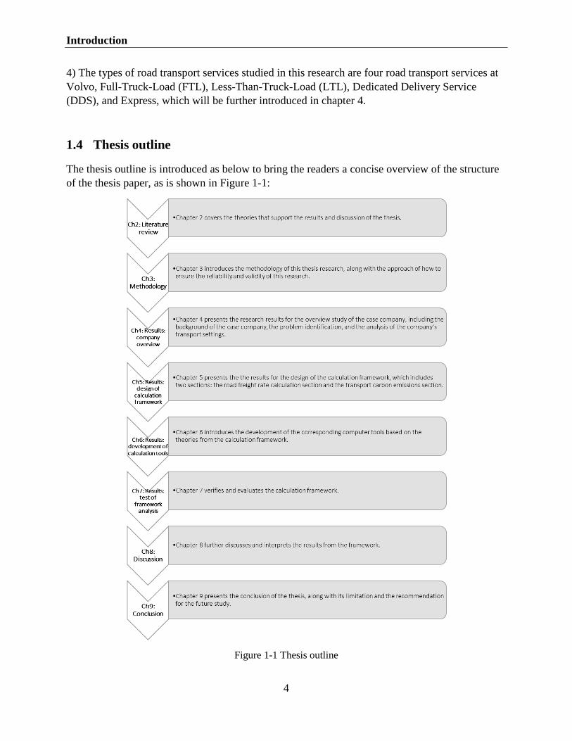
1.4 Thesis outline
The thesis outline is introduced as below to bring the readers a concise overview of the structure
of the thesis paper, as is shown in Figure 1-1:
Figure 1-1 Thesis outline

Literature review
5
2 Literature review ---------------------------------------------------------------------------------------------------------------------
This chapter covers the theories that support the results and discussion of the thesis. In the first
section, the cost breakdown theory is introduced. In the second section, existing studies on the
estimation of road freight costs are reviewed. In the next section, other factors that might
influence the road freight rate are discussed. The second last section presents existing theories
and methods of estimating carbon emissions from road transport and the last section briefly
introduces VBA which is applied in this research.
---------------------------------------------------------------------------------------------------------------------
2.1 Cost breakdown theory
In order to identify the cost elements that contribute to the overall road freight rate, cost
breakdown theory is applied. As one of the most common methods for analyzing the cost, cost
breakdown can be implemented by developing a cost breakdown structure, which is used to break
down the various elements of cost (Garrett, 2008).
Figure 2-1 shows a basic cost breakdown structure. When implementing the cost breakdown
method, based on the basic theory that “price (rate) is made up by the component of cost and the
component of profit”, the first breakdown process can be made which breaks the overall price or
rate in into two components: cost and profit. Then, following the breakdown structure, a second
breakdown can be made which specifically focuses on dividing the cost component into two
categories: direct cost and indirect cost. While direct cost refers to the cost that is directly
associated with a specific cost item (e.g. a task, service, or material), the indirect cost cannot be
directly tied to a specific cost item (Barnes & Langworthy, 2004). The cost elements that belong
to direct cost or indirect cost can vary from case to case. However, some cost elements should
normally be included in either one of the two categories, such as labor cost, material cost,
subcontracting cost, overhead, other direct cost (ODC), and governance and administration
(G&A) (Garrett, 2008). Even though reaching this third layer of the cost breakdown structure
could be detailed enough from some cost breakdown cases, for some other more complex cases, a
third breakdown can be made to determine the more reasonable cost elements for estimation and
calculation, as is shown in the fourth layer of Figure 2-1.

Literature review
6
Figure 2-1 A structure of cost breakdown (Garrett, 2008)
When conducting a cost breakdown analysis, three principles should be considered to ensure the
reasonableness and validity of the newly broken-down cost elements:
Is this cost element generally recognized as necessary in conducting the business
operation in this specific case?
Is this cost element consistent with sound business practice, law, and regulation?
Is this cost element duplicated with other cost elements, either partially or entirely, i.e.
will it result in double-counting of cost?
Following those three principles, the determination should be made about whether a certain cost
element is qualified for being a result of a specific cost breakdown process (Garrett, 2008).
2.2 Estimation of road freight cost
2.2.1 Cost classification
Cost elements in road freight transport have different attributes so that they can be classified in
different ways. Some common types of cost elements in the literature are summarized below and
will be further explained.
1) Fixed and variable costs
2) Direct and indirect costs
3) Internal and external costs
Classifying the costs elements into fixed costs and variable costs is the most common method in
existing studies on road freight cost estimation (Holguin-Veras, Gonzalez-Calderon, Lawrence,
Brooks, & Tavasszy, 2013; Berwick & Farooq, 2003; Litman, 2009; Sternad, 2019; Casavant,
1993). Variable costs are incremental costs that can go up and down according to the change in
company activities or consumptions. In the context of road freight transport, variable costs are
directly influenced by the vehicle mileage, such as fuel cost and tire cost. Variable costs are also
called marginal costs, indicating the cost value could increase or decreased based on the amount

Literature review
7
of output. (Holguin-Veras, Gonzalez-Calderon, Lawrence, Brooks, & Tavasszy, 2013). On the
contrary, fixed costs do not change depending on the level of output and will incur during the
decision period even the output is zero. Typical fixed costs are truck investment, insurance
(Holguin-Veras, Gonzalez-Calderon, Lawrence, Brooks, & Tavasszy, 2013). Rastogi and Arvis
(2014) and Sternad (2019) apply this classification method in the analysis of transport cost
structure.
Direct costs are the costs that can be directly allocated with a specific cost item such as service,
material, while indirect costs cannot be directly associated with a specific cost item (Holguin-
Veras, Gonzalez-Calderon, Lawrence, Brooks, & Tavasszy, 2013). Litman (2009) explains
indirect costs with indirect impacts which means there are several steps between activity and
ultimate results. The cost-breakdown method proposed in Garrett (2008) divides the total cost
into the direct and indirect costs.
Internal costs are the costs borne by the transport users, while external costs are the cost to
society. External costs occur when the activities performed by one group influence another group
and this influence is not fully considered by the first group (Ortolani, Persona, & Sgarbossa,
2011). Typical external costs caused by road transport include noise and carbon dioxide
emissions (Ortolani, Persona, & Sgarbossa, 2011; Litman, 2009).
The three methods are independent and can be combined when using. For example, Jacyna and
Wasiak (2015) applied a classification method with two criteria. The costs incurred in road
transport are first divided into fixed costs and variable costs. Within each category, the costs are
further divided based on direct and indirect costs. Litman (2009) divided cost elements into four
categories: internal fixed costs, internal variable costs, external fixed costs, and external variable
costs.
To summarize, all three methods are implemented in previous studies and there are no strict rules
on choosing which classification method. The distinction between fixed and variable costs is
more commonly used. From a business perspective, the freight rate consists of internal costs
while the environmental performance consists of external costs.
2.2.2 Cost elements and estimation methods
The academic studies on estimating road freight costs from a business perspective are limited.
Casavant (1993) proposed the basic theory of calculating costs and applied it to trucking costs.
Eleven cost elements were discussed in this article where the labor cost, cost of capital, overhead,
and depreciation were clearly defined in particular. However, Casavant (1993) only stated
theories of estimating cost elements without providing any practical formulas or case studies. The
research of Berwick and Farooq (2003) is a further development of theories proposed by
Casavant (1993). It considered the same cost elements as Casavant (1993) and applied the
theories to develop the calculation methods for each of the elements. More importantly, a stand-
alone truck costing model was developed using Microsoft Visual Basic for Window which can
not only estimate trucking cost based on data input but also make sensitivity analysis of several
parameters, such as fuel and trip distance (Berwick & Farooq, 2003). However, the calculation
method and the software model were developed in the context of the US and the article didn’t test
Literature review
8
the model with an example. Barnes and Langworthy (2004) studied several variable costs (fuel
cost, repair and maintenance, tires, and depreciation) in operating personal vehicles and trucks.
Although the number of researched cost elements was limited, more detailed analysis and data
input were given. Finally, a comparison of each cost element among three types of vehicles
(automobile, van, commercial truck) was made. The commercial truck was shown to be the most
expensive for each of the researched cost elements (Barnes & Langworthy, 2004). Jacyna and
Wasiak (2015) considered 14 different cost elements when estimating road transport costs. The
calculation formulas for vehicle depreciation, cost of capital, ecological cost was given, while the
calculation theories for other cost elements were discussed. A case study was conducted that
compared each cost element as well as the total cost of using four types of the truck to carry the
same shipment from Mszczonów (PL) to Hamburg (DE). Kovács (2017) considered six cost
elements when calculating the cost to fulfill a road transport task. The calculation model has two
major differences compared with previous literature. The first is the cost incurring during waiting
time at stops is considered. The second is the cost of capital is further divided into two categories
based on if the operator owns the truck or leases the truck, which can make the model applicable
to assist the decision-making on self-operation or outsourcing (Kovács, 2017). Sternad (2019)
calculated the truck cost over one year instead of for each shipment task. The total cost was
divided into 8 different elements with definitions and calculation methods. Then the cost
structure was presented, and relations between average cost and vehicle mileage were analyzed.
The cost elements considered in the above literature and whether the corresponding calculation
methods are given are summarized in Table 2-1.

Literature review
9
Table 2-1 Summary of cost elements in the literature
Cost Elements Casavant (1993)
Berwick & Farooq (2003)
Barnes & Langworthy
(2004) Jacyna & Wasiak
(2015) Kovács (2017) Sternad (2019)
Inclusion
Calculation method Inclusion
Calculation method Inclusion
Calculation method Inclusion
Calculation method Inclusion
Calculation method Inclusion
Calculation method
Cost of capital × × × × ×
Vehicle registration fee × × × × ×
Vehicle insurance × × × × × ×
Vehicle tax × × × ×
Vehicle garage/housing ×
Vehicle depreciation × × × × × × × × ×
Periodical inspection ×
Maintenance and repairs × × × × × × × × × ×
Fuel cost × × × × × × × × × ×
Wear of tires × × × × × × ×
Ecological fee × ×
Park cost × ×
Road toll × × × × × ×
Driver labor salary × × × × × × × ×
Driver night cost ×
Driver diets and accommodation × × ×
Driver overtime ×
Overhead × × × × ×
Cost during the waiting time × ×

Literature review
10
From Table 2-1, it could be seen that fuel cost, maintenance, and repair cost are considered in all
literature. Driver cost, tire cost, depreciation, cost of capital, insurance, and tax are considered in
most literature. Although most literature considers driver cost, only two of them give more
detailed information on how it is structured (Kovács, 2017; Snyder, 2019). Period inspection and
the ecological fee are considered only by Jacyna and Wasiak (2015) and other literature
considers them as part of maintenance and road toll. Overhead as an important indirect cost, is
included by three articles. Cost during waiting time is only considered by one article although it
is an important cost component during a road shipment.
To summarize, this section reviews current literature in comprehensively estimate road freight
cost from a business perspective. The number of articles in this area is quite limited. Different
articles comprise different cost elements, but none of them include all the cost elements and
provide practical calculation methods for each cost element.
2.2.3 The cost structure of road freight transport
Sternad (2019) has analyzed 8 cost elements of road freight transport over one year in Slovenia.
The result shows that fuel cost takes the largest share of the total cost, from 27% to 31%
depending on the annual mileage of the vehicle. The toll cost and labor cost come after fuel cost
and both of them account for around 20% of the total cost. The fourth-largest part is the indirect
cost followed by depreciation cost. The least three cost elements are maintenance, insurance, and
registration, all of which make up less than 5% of the total cost (Sternad, 2019). The article
compared the cost structure of vehicles with four different levels of yearly mileage. The result
shows there is a slight difference in the cost structure. For example, with the increase of yearly
mileage, the share of fuel cost increases a bit, while the depreciation cost drops slightly.
A survey conducted by Rastogi and Arvis (2014) shows the cost structure of four Kyrgyz carriers
when operating road transport in Europe. The survey comprises four cost categories, fuel costs,
labor costs, capital costs, and other costs. Results show the average cost of the four carriers
differs from region to region. For example, the fuel cost is the largest share in Lituania, Poland,
Hungary, the Czech Republic, Slovak Republic, Bulgaria, and Romania, accounting for more
than 30% of the total cost. However, in EU 15, the labor cost is the largest cost element and in
Russia, the capital cost takes the most share (Rastogi & Arvis, 2014).
Jacyna and Wasiak (2015) analyzed the cost structure of a road shipment from Mszczonów (PL)
to Hamburg (DE) with four different vehicles. The fuel cost is the largest part regardless of which
type of vehicle is used, accounting for around 35% of the total cost. The second and third are
labor costs and road fees with a share of 27% and 14% to the overall costs respectively. The
result clearly shows the influence of the vehicle on the cost structure. For example, the average
fuel consumption of vehicle 4 for running 1 km is 5 liters less than vehicle 1, which results in a
saving of 300 EUR in the fuel cost.
The analysis made by Maibach, Peter, and Sutter (2006) also addressed the different cost
structures of different countries. In EU15, the labor cost takes the largest proportion while the

Literature review
11
fuel cost comes to the second. However, in Eastern Europe, the fuel cost accounts for the most
share, and labor costs come to the second. This finding is consistent with the result obtained by
Rastogi and Arvis (2014). Besides, Maibach, Peter, and Sutter (2006) presented the operating
distance also influences the cost structure of road shipment. The data from Germany shows the
share of the labor cost of the truck carrying short-distance tasks is 49.6% to the total cost, while
the number is 38.7% for the truck carrying long-distance tasks.
In addition to the comparison of each specific cost element, the comparison between fixed and
variable costs is made in some studies. Sternad (2019) stated the variable costs make up around
60% in total costs and its share increases to 70% with the yearly mileage of the truck increasing
from 96,000km to 144,000km. Cowie (2009) also stated the fixed costs in road freight transport
tend to relatively low, at around 25% of the total costs. The figure provided by Cowie (2009) also
included the costs at the terminal which are not included in this thesis. Besides, the share fixed
costs in LTL transport is a bit higher compared with in FTL because of the time spent on serving
the depots (Cowie, 2009). In contrast, Kovács (2017) got a different conclusion. By comparing
the variable costs per mile calculated by their methods with the total road freight cost per mile
obtained from a routinely used external source, they concluded variable costs are 43% of the total
costs.
To summarize, there is no consistent conclusion on how the cost structure of road freight
transport looks like because it is impacted by factors such as regions, vehicles, shipments, yearly
mileage. However, it could still be concluded that fuel cost, labor cost. Toll cost varies based on
the operating countries. As for the comparison of fixed and variable costs, there is no consensus
on which overweighs the other.
2.3 Other factors that influence freight rate
2.3.1 Trade imbalance – backhaul problem
Backhaul means to haul a shipment or empty trailer/container back from the destination to the
origin (Reichert & Vachal, 2000; Fekpe, Alam, Foody, & Gopalakrishna, 2002). In reality, the
backhaul doesn’t need to strictly follow the loaded trip. Instead, the backhaul could be more
flexible, as indicated in Figure 2-2.The backhaul problem is a common phenomenon in road
freight transport because the volume of the transported goods is not balanced among locations so
that the transport flow is dominant in one direction. Due to this imbalanced flow, carriers may
find it is difficult to organize the flow for the return trip (Demirel, Van Ommeren, & Rietveld,
2010).

Literature review
12
Figure 2-2 Illustration of backhaul planning
Some literature has recognized the influence of the backhaul trip on the front-haul prices. Wilson
(1987) proposed that the probability of organizing backhaul flow varies across regions and
markets and the front-haul prices should cover the backhaul costs. If there is a large possibility of
organizing backflow, the front prices should be adjusted downward. Demirel, Van Ommeren, and
Rietveld (2010) also stated positive backhaul prices should be paid to carriers as a compensation
for the expected search time when organizing the backward transport flow. A researched example
found the German companies normally pay for the increased transport costs between Germany
and the Netherlands because Germany companies import more goods from the Netherlands
(Demirel, Van Ommeren, & Rietveld, 2010). This interesting finding further supports that the
imbalanced goods flow will impact the road freight rate.
Cooper, Woods, and Lee (2008) summarized four methods of accounting backhaul influence
when analyzing the environmental impacts of truck transport:
1) Stated the backhaul is not included
2) Assume a backhaul factor of 30% - 60% of the energy use and emissions of the front-haul
3) Provide models for partially loaded or empty vehicle
4) Assume the backhaul is equivalent to front-haul
To summarize, the backhaul problem is common in the transport network and has a direct
influence on the front-haul rates. Therefore, it should be considered, although none of the
literature reviewed in section 2.2.2 has taken it into account.
2.3.2 Stakeholder interaction
The road freight rate is the outcome of negotiation between buyer companies and transport
service providers. Purchasing negotiation is affected by three variables: time, power, and relation
(Shin & Pak, 2016).
Information is the core of negotiation. Better use of information is more likely to bring a mutually
beneficial agreement. The information in negotiation could be assessed from three perspectives.
The first is the quality of information which is of great importance because it influences the risk
level. High-quality information could reduce uncertainties and lead to a better decision. The
second is the quantity of information. Adequate information will enable control over the
negotiation process. The more information a party has, the more possibility it has to win the
negotiation. The last is the flow of information, which indicates the symmetry of information.

Literature review
13
There is an idea that symmetric information flow could facilitate negotiation because an equal
exchange of information could satisfy both parties (Shin & Pak, 2016).
Power is interpreted as the relative dependency between parties. For example, if the supplier is
more dependent on its buyer than the buyer on the supplier, the buyer has more power over the
supplier. The power shows to what extend one party can influence and be influenced by the
counterparty (Batt, 2003). Power is critical to the outcome negotiation because the party with
more power can force the other one to make a concession even though the other tends not to
concede. There are five sources of power in the negotiation process. The first one is expert power
which means when a party has expertise in technical and administration that makes it difficult to
replace, the party poses expert power. The second is referent power. It is decided by the
attraction of one party to the other party. This attraction comes from mannerisms, friendliness,
and desire to build up a relationship. The third is the legitimate power which comes from the
relative position of two parties. The fourth is reward power which comes from the potential
benefits such as additional resources if an agreement is reached. The last one is coercive power
which in contrast comes from potential punishment (Shin & Pak, 2016).
Time is also an important constraint in negotiation. Time pressure could facilitate negotiating
parties to concede to reach an agreement but is also negatively influence the quality of the
outcome (Shin & Pak, 2016).
As an outcome of purchasing negotiation, road freight rates are also affected by these three
factors. Therefore, it is not enough to understand the freight rate simply from the accounting
perspective. The impact of business operations should also be considered.
2.3.3 Size of carriers
Even carry the same shipment between the same locations with the same equipment, the freight
rate could also vary across different carriers depending on the size of the transport company.
Casavant (1993) stated the cost per mile of road freight shipment would decrease with the
increase in the firm size. The reason for this pattern includes a larger firm is more likely to buy
the insurance policy or purchase truck fleets with higher discounts. Also, larger companies have
more demands, meaning it is easier for them to organize transport flow in backhaul (Casavant,
1993). This phenomenon could be interpreted by the impact of economies of scale (Cowie, 2009).
The long-run average cost (LRAC) at first falls with the increase of firm size which results from
bulk buying, improved productivity, financial economies. However, after falling to an optimum
level, the average cost will rise with the increase of firm size because of more management
layers, decreasing return to scale (Cowie, 2009).
Figure 2-3 Long run average and marginal costs (Source: Cowie (2009))

Literature review
14
As stated in section 2.3.1, the probability for backhaul transport will influence the freight rate. In
the LTL industry, the average cost in the long-run declines at a diminishing speed with the
increase of firm size (Giordano, 2008). Miller and Muir (2020) summarized the reasons why
larger carriers can operate road transport in lower average costs in the FTL industry. The first
reason is a larger carrier can better pool demand variance which means compared with small
carriers, large carriers can achieve the same level of capacity availability with reserving a smaller
marginal equipment capacity. The second reason is larger transport companies are more
applicable to invest in information technologies and the high demands can ensure the utilization
of IT/IS. The third reason is larger carriers have more ability and more likelihood to cooperate
with shippers that have more volume. The last reason is carriers with large size can better achieve
the economies of density by reducing the waiting time for drivers to be assigned to the next
shipment (Miller & Muir, 2020).
2.4 Carbon emissions calculation for road transport
Many studies have been conducted regarding how to effectively calculate road transport carbon
emissions. While some of them focus on the on-road section carbon emissions of the transport
process, others focus on the handling operations section carbon emissions of the transport
process.
A method called Methodology for calculating transportation emissions and energy consumption
(MEET) is designed to calculate carbon emissions and energy consumption for road
transportation. The final result produced through this method is in the metric of “the rate of
carbon emissions per kilometer”. By classifying the vehicles into several categories based on
their weight, the rate of emissions per kilometer is assigned to each specific category of the
vehicle based on an average vehicle speed-dependent regression 𝑒𝑟(𝑣) = 𝐾 + 𝑎𝑣 + 𝑏𝑣2 + 𝑐𝑣3 +
𝑑𝑣−1 + 𝑒𝑣−2 + 𝑓𝑣−3, where 𝑒𝑟(𝑣) is the rate of carbon emissions for an unloaded goods vehicle
on a road with zero gradients. The parameters K, and a to f are predefined coefficients whose
values vary from one category of vehicle to another and have been specified according to each
category. Meanwhile, for this method, there are also two other sets of coefficients that
respectively work for when the road gradient effect and loading effect are taking into account.
However, as this MEET method is designed in 1999, the applicability of those coefficients to be
used today is uncertain; also, this method has not stressed the carbon emissions impact from
different types of fuel for the vehicle (Demir, Bektas, & Laporte, 2014). Another method for
calculating the road transport carbon emissions, the Ecological transport information tool
(ECOTRANSIT), provides a calculation approach that has taken the upstream energy
consumption portion into account, which is the energy consumed during the production of the
fuel used in road transport. The calculation approach can be performed in three processes. The
first process is to calculate the final energy consumption as “per net ton kilometer
(𝐸𝐶𝐹𝑡𝑜𝑛 𝑘𝑖𝑙𝑜𝑚𝑒𝑡𝑒𝑟)” by the equation 𝐸𝐶𝐹𝑡𝑜𝑛 𝑘𝑖𝑙𝑜𝑚𝑒𝑡𝑒𝑟 = 𝐸𝐶𝐹𝑘𝑖𝑙𝑜𝑚𝑒𝑡𝑒𝑟/(𝐶𝑃 ∗ 𝐶𝑈), in which
𝐸𝐶𝐹𝑡𝑜𝑛 𝑘𝑖𝑙𝑜𝑚𝑒𝑡𝑒𝑟 refers to the “final energy consumption per net ton kilometer”, CP refers to the
“payload capacity” and CU refers to the “capacity utilization”. The second process is to calculate
the “upstream energy consumption per net ton kilometer (𝐸𝐶𝑈𝑡𝑜𝑛 𝑘𝑖𝑙𝑜𝑚𝑒𝑡𝑒𝑟)” by the equation
𝐸𝐶𝑈𝑡𝑜𝑛 𝑘𝑖𝑙𝑜𝑚𝑒𝑡𝑒𝑟 = 𝐸𝐶𝐹𝑘𝑖𝑙𝑜𝑚𝑒𝑡𝑒𝑟 ∗ 𝐸𝐶𝑈𝐸𝐶, in which 𝐸𝐶𝑈𝐸𝐶 refers to “the energy related
Literature review
15
upstream energy consumption”. The last process is to calculate the total energy consumption as
𝐹(𝐷, 𝑀) = 𝐷 ∗ 𝑀 ∗ (𝐸𝐶𝐹𝑡𝑜𝑛 𝑘𝑖𝑙𝑜𝑚𝑒𝑡𝑒𝑟 + 𝐸𝐶𝑈𝑡𝑜𝑛 𝑘𝑖𝑙𝑜𝑚𝑒𝑡𝑒𝑟), in which M refers to “the mass of
freight transported (ton)”. In this method, the effect of the loading factor has been taken into
consideration and integrated into the calculation process, while the effects of gradient and driving
patterns are not included. This method can be a good source to calculate the carbon emissions for
road transport if the upstream energy consumption carbon emissions should be included (Demir,
Bektas, & Laporte, 2014). One method that has been used mainly by the business operators of
transport service is the Network for Transport Measures (NTM). In this method, an assumption
has been stressed that all carbon is transformed into 𝐶𝑂2. With this assumption the carbon
content (in mass-%) is multiplied with the fuel density and the molecular weight relations,
(12+16+16
12=
44
12(as the molecular weight of 𝐶𝑂2 = 44 and Carbon = 12)), the emission factor
can be acquired with a unit of “kg/l”. Then using the emission factor to multiple with the fuel
consumption (liter) during the trip, the figure of the carbon emissions during this specific trip can
be obtained (Network for Transport Measure, 2015). This method gives the flexibility to whether
the calculation should take other effective factors such as gradient and loading into account since
all the impacts of those factors can be reflected by the corresponding figure of fuel consumption.
There are also some other studies focusing on the warehousing and transshipment processes
section carbon emissions. Rüdiger, Schön, and Dobers (2016) conducted a study aiming at
defining a comprehensive carbon emissions assessment method for the logistics facilities and
handling processes. After clearly determining the system boundaries and scope for the logistics
facilities and the handling processes, a carbon emissions calculation theory based on the
multiplied result of the measured (statistical) values on the quantities of energy and resource
consumption and the emission conversion factor is established. Thereafter, the total carbon
emissions result can be distributed to each handling process and logistics facility.
2.5 Visual Basic for Applications
Visual Basic for Applications (VBA) is an object-oriented programming language developed by
Microsoft that can be integrated with all Microsoft Office applications (Mansfield, 2013). In this
research, only the VBA integrated within Microsoft Excel will be focused. With the help of
VBA, many tasks could be accomplished, such as creating custom command, creating complete
and macro-driven functions (Walkenbach, 2013). VBA has the following advantages that make it
popular:
1) VBA is a complete programming language, which means it can recognize all variable types,
handle tasks like working with strings, managing dynamic fields, and applying a recursive
function (Kofler, 2008). It is applicable to achieve the functions needed in this research.
2) VBA can be accessed and edited with Excel and it also has a good interaction with Excel.
Currently, most data and process related to purchasing at the case company is stored in Excel.
Therefore, tools developed with VBA could be integrated with the current business process
more easily.
Literature review
16
3) VBA is event-oriented. When using VBA, developers don’t need to worry about the
management of events. They only need to develop the macros and the macros will be
triggered automatically when related buttons are clicked (Kofler, 2008). This feature reduces
the difficulty in creating the interaction between users and tools.

Methodology
17
3 Methodology ---------------------------------------------------------------------------------------------------------------------
In this chapter, the methodology of this thesis research will be presented. In the first section, the
research outline of this thesis is demonstrated. Then, following the research onion model and
based on the research questions of this thesis, the research elements such as research approach,
methodological choice, research strategy, time horizon, and data collection will be discussed.
Besides, a comprehensive research outline along with the validity and reliability of this research
will be interpreted.
---------------------------------------------------------------------------------------------------------------------
3.1 Research outline
According to the research plan and the sequence of how this thesis is conducted, the thesis
research is divided into four stages and seven processes, as is shown in Figure 3-1. The first stage
is the theoretical part of the thesis which is designed to answer the first and the second research
question. The first process in the first stage is corresponding to the first research question, while
the second process is designed for the second question. The third stage answers the third research
question. The last two stages are the case study part in which the estimation framework and tools
will be tested with the data from the case company, Volvo.
Figure 3-1 Research outline

Methodology
18
3.2 The research onion model
The research onion model is a methodological model for academic research which contains five
layers of different research elements: research approach, methodological choice, research
strategy, time horizon, and data collection. For each layer, it stands for a stage of methodology
related choice that a researcher must carefully consider and select to implement the suitable
actions and secure the credibility of the research. As is shown in Figure 3-1, beginning from
looking into the topmost layer of this “research onion” (the research approach), then moving to
the more inside layers sequentially, the results acquired from this process would contribute to the
logical and effective methodology design of research (Saunders, Lewis, & Thornhill, 2009).
Figure 3-2 Research onion model (Saunders, Lewis, & Thornhill, 2009).
3.3 Research approach
The research approach that can be applied to research could be inductive or deductive, depending
on the research purposes, questions, limitations, and so on (Saunders, Lewis, & Thornhill, 2009).
Inductive approach refers to the research approach whose flow is generally from specific to
generic, i.e. starting from the study of specific data to findings of theory and conceptual
framework. In addition, the inductive approach can be conducted when the prior theoretical
knowledge is limited. The deductive approach refers to the research approach whose flow is, on
the other hand, from generic to specific, i.e. start with theory and then continue to the research
questions which are tested by data. As a vital prerequisite for this approach, sufficient prior
theoretical knowledge is needed (Saunders, Lewis, & Thornhill, 2009).

Methodology
19
Considering the research questions of this thesis and the possible prior theoretical knowledge that
could be acquired for this study, a deductive approach is applied to this thesis research. Because
the literature review and information acquired from Volvo have enriched the researchers with
sufficient prior theoretical knowledge regarding different sections of this research, such as cost
breakdown theory, road transport services, and calculation methods for each identified cost
element. Starting with those theories and methods, the researchers design and implement their
framework for answering the research questions, together with the verification processes by using
the appropriate data. To apply the deductive research approach, the thesis will start with studying
the theories on estimating freight rate and carbon emissions of road transport. Then, a general
theoretical framework will be built up together with user-friendly tools based on the framework.
The part is generic and corresponds to the first and second research questions. After that, the
research narrows down to a specific part which is the test and verification of the framework and
tools by data the case company Volvo Group.
3.4 Methodological choice
For the methodological choice of research, quantitative methods and qualitative methods could be
the options to apply. When it comes to the methodological choice for specific research, the
researchers need to make decisions on whether both of the methods are in need for the study or
only one of them is in need; if both quantitative and qualitative methods are in need, should them
weigh equally or should one of them dominate the other. For this decision of method selection
and combination, there are three types of choice:
mono-method: apply either quantitative methods or qualitative methods
mixed-method: equally apply quantitative methods and qualitative methods, such as in the
process of data collection and data analysis; compensate for the limitation of each other
multi-method: applying both quantitative and qualitative methods for the research.
However, during some processes such as data collection and data analysis, only one kind
of method will be applied (Saunders, Lewis, & Thornhill, 2009).
In addition, while mixed-method uses both the quantitative methods and qualitative methods all
the way together to establish a particular and single set of data and findings, the multi-method is
implemented in the research which is commonly divided into different sections, and each section
may focus on either of the two methods to produce a set of data and findings for that stage (Uwe,
2011).
As is shown in Figure 3-1 in Section 3.1, there are seven research processes for this thesis. For
each process, at least one of the methods between quantitative methods and qualitative methods
should be applied. The second and sixth processes will apply quantitative research methods
because the second process will reflect the second research question which is the calculation
methods for cost elements and the sixth process is the test of the framework. The other processes
will apply qualitative methods. As a result, the methodological choice of multi-method will be
applied.

Methodology
20
3.5 Research strategy
Research strategy refers to what type of structure and research design will be implemented in a
research study in order to achieve the research objective and answer the research questions.
Typical research strategies for academic research include experiment, survey, case study, action
research, grounded theory, ethnography, archival research, and narrative inquiry. In some cases,
there can be more than one research strategy selected for certain research (Saunders, Lewis, &
Thornhill, 2009). With the consideration of the research purpose, the selection of the research
approach, and methodological choice, the research strategy of case study is selected for this thesis
research.
The research strategy of case study is defined as an empirical inquiry that examines a
phenomenon in its real-life context, especially when the boundaries between the phenomenon and
context are not evident (Yin, 2017). In this thesis research, which is exploratory research of
designing a theoretical calculation framework with the further aim to resolve the demands and
problems from the case company, the research strategy of case study enables the researchers to
build up the investigation from multi-perspectives, select the suitable methods for this specific
phenomenon, as well as examine the findings in the real-life context of the research scope
together with the conclusions that have the potential to be generalized (Baxter & Jack, 2008).
The four transport services at Volvo are selected as cases, which is a multiple-case design (Yin,
2017). They are Full-Truck-Load (FTL), Less-Than-Truck-Load (LTL), Dedicated Delivery
Service (DDS), and Express. They will be further introduced in chapter 4. The four cases will be
studied and investigate following the order:
1) Understand how the services are organized and what are the features of each of them.
2) Collect the tested data of transport services
3) Test the framework and tools with data of the four cases
4) Discuss the results of each case and make a comparison among all the cases
3.6 Time horizon
The time horizon of the research refers to the constraint of time scope for conducting the
research, which can be determined as cross-sectional or longitudinal. While cross-sectional
horizon focuses on a time scope of a specific time and the findings within that scope, longitudinal
horizon focuses on a time scope of a certain period when data collection and analysis should be
continued and examined over time (Saunders, Lewis, & Thornhill, 2009). When it comes to the
time horizon for this thesis research, the cross-sectional horizon should be applied, and the time
scope for the researchers to conduct this study is limited to the specific period for this thesis.
3.7 Data collection
In the process of data collection, the data in need for this research is divided into two categories:
primary data and secondary data. Primary data refers to the information that the researchers

Methodology
21
gather through firsthand. Secondary data refers to the information from secondary sources, which
is not directly acquired by the researchers (Rabianski, 2003). The methods for acquiring primary
data and secondary data are also different. In the following sections 3.7.1 and 3.7.2, the specific
methods for acquiring the primary data and secondary data in need of this thesis research will be
presented and discussed.
In addition, and for emphasis, data collection in this section refers to not only the data for
developing the calculation framework, but also the data in need for testing and verifying the
framework, as well as the data for resolving the problems and demands from the case company
Volvo Group.
3.7.1 Primary data
The primary data in need for this thesis research is mainly from the following three aspects:
1) Data, information, and theories that are needed for designing the calculation framework,
regarding not only the cost elements but also the calculation method for each cost element
2) Supportive data as data input to test and verify the calculation framework
3) Critical data and information to resolve the specific problems and demands from the case
company
To acquire the above vital primary data, the method of interview will be applied.
Interview
According to (Kajornboon, 2005), interview is an efficient and common-used way to collect data
and acquire knowledge from individuals. There are three types of interviews: structured interview
(also called standardized interview), semi-structured interview, and unstructured interview
(Kajornboon, 2005). Structured interview refers to “the interview in which all respondents are
asked the same questions with the same wording and in the same sequence”. Structured interview
gives more control to the researchers over the topics and the format of the interview (Kajornboon,
2005). During a semi-structured interview, interviewers have a set of questions to address, but the
questions can be rephrased, or additional questions can be added in the process. This type of
interview gives interviewers more opportunities to probe the knowledge and opinions of
interviewees (Kajornboon, 2005). When it comes to the unstructured interview, interviewers
mainly take the role of listeners while interviewees take the lead and speak freely and openly.
This method is particularly suitable at the beginning stage when interviewees have little
knowledge (Kajornboon, 2005).
In order to acquire the primary data mentioned above, several semi-structured interviews and
unstructured interviews have been arranged with Volvo personnel from the functions of Logistics
Purchasing (LP) and Footprint Design(FD). The selection of the interviewees is based on their
expertise and availability according to schedule, as is shown in Table 2-1.

Methodology
22
Table 3-1 Contextual information of the conducted interviews
No. Function/
Team
Respondents Interview type Subject Duration
1 LP Logistics
purchaser
Unstructured
interview
General information about
the Volvo Group Trucks
Operations and the
department of LP, along with
the demand from LP for this
study
60 min
2 FD Supply chain
analyst
Unstructured
interview
General information about
FD, along with the demand
from FD for this study
60min
3 FD Supply chain
analyst
Unstructured
interview
Information and settings
about the five types of
transport set-ups within
Volvo
45min
4 LP & FD Logistics
purchaser &
Supply chain
analyst
Unstructured
interview
Some empirical figures,
findings, and facts about the
transport settings and
operations within Volvo
Group
60min
5 LP & FD Logistics
purchaser &
Supply chain
analyst
Semi-structured
interview
Some empirical figures,
findings, and facts about the
transport settings and
operations within Volvo
Group
40min
Unstructured interviews were arranged at the very initial phase of the thesis research because the
researchers needed to build up the fundamental knowledge and understanding of concepts within
Volvo Group and the two functions. Through those unstructured interviews, primary data such as
the demands and problems from the two functions, the information and definitions of the five
Volvo transport set-ups, and some proposed cost elements have been understood and acquired.
After the initial phase, semi-structured interview was conducted to acquire the primary data
which is more topic-specific and targeted-based, such as some empirical figures as input for the
calculation framework and suggestions for designing the calculation framework. The question list
for the semi-structured interview is presented in Appendix C: Question list for semi-structured
interview. By having accomplished each specific interview, information and data have been
collected and categorized, while some of the results directly contributed to the thesis research,
others have turned out to be the questions for the next interview in which they would be
discussed further.
3.7.2 Secondary data
The secondary data in need for this thesis research is mainly from the following four aspects:

Methodology
23
1) General information about the case company Volvo Group, logistics purchasing function, and
footprint design team.
2) Information about transport services at Volvo
3) Some empirical figures, findings, and facts about the transport situations and operations
within Volvo Group
4) Information regarding the general research background and methods
In order to acquire the above secondary data, the data collection process will start from the
following aspects:
Literature review
Literature review is a process where researchers describe prior studies and evaluate current states
to further motivate the research objective and justify research questions. It is a good way to
provide an overview of the researched area or issue, reveal the gaps that need further
investigation, and address research questions (Snyder, 2019). In this thesis research, literature
review is conducted to present the general research background, identify suitable research
methods, and support the design of the calculation framework. Data sources such as Google
Scholar, ScienceDirect, and SpringerLink are used for the literature review to collect the
materials of dissertations, books, academic journals, commercial and governmental reports, etc.
Keywords related to cost breakdown theory, cost elements, road freight rate, transport carbon
emissions, etc., are used to search the materials during the literature review process.
Additional external data sources
To acquire the vital secondary data of some specific figures, regulations, and route information,
additional external data sources rather than the ones for literature review have also been used,
such as some website (e.g. European Commission websites) and official databases and statistics
(e.g. EU statistics database). In addition, a geography route engine database, PTV Map & Guide,
is used in this research to provide the up-to-date route data for testing and verifying the
calculation framework.
Internal data sources from Volvo Group
For some specific secondary data regarding the case company Volvo Group and its business
operations, the internal data sources such as some Volvo internal database, materials (e.g. reports,
slides, contracts), bid/price records, and invoices will be the sources to acquire such data and
information. However, because some of such secondary data is the confidential data of Volvo
Group and is not allowed to share with the public, in this thesis paper, the researchers will put
such data in anonymity.
3.8 Reliability and validity
According to Saunders et al. (2009), reliability and validity are the two basic pillars that need to
be considered when assessing the quality and applicability of research with both quantitative and
qualitative methods. While reliability refers to “the absence of differences in the results if the
Methodology
24
research is repeated”, validity refers to “the extent to which the research findings accurately
reflect the phenomena under study” (Hussey & Collis, 2013). To ensure the reliability and
validity of this thesis research, triangulation will be implemented. Triangulation refers to
applying multiple sources of data, different research methods, and/or more than one researcher to
investigate the same phenomenon in research (Hussey & Collis, 2013).
Processes have been taken to secure the reliability of the research. First, for each transport service
at Volvo, at least 8 transport shipments have been used in testing. In total, 8 samples with 26
shipments are randomly selected and tested. The verification of multiple increases the reliability
of the research. Second, when designing the calculation framework, the majority of the methods
and theories applied are the common and public ones that are accessible through open sources,
e.g. research paper, public statistics, databases, reports. Third, for the data and information
acquired from the internal sources of Volvo, a track of record for the relevant sources is noted,
including interview questions and interviewers, databases, reports, slides, etc. This makes the
verification and reproduction of the research feasible in the future by other researchers. Besides,
the two researchers for this thesis have also cross-checked each section with the same set of
research methods that have been applied, which works as an internal check process for reliability.
Last but not least, an outline for this research is demonstrated in section 3.1 as a clear process
map for other researchers to refer to when replicating a study.
When it comes to ensuring the validity of this research, methods have been used by the
researchers to secure the research measures that are intended to be studied. For example, the
output of the framework is tested with the true bid price from the case company Volvo. The
differences between the estimated result and the true bid price are shown and analyzed in chapter
7 and chapter 8. Besides, more than one source has been applied when collecting the data,
information, and theories to ensure that the result of the collection is error-free and valid. In
addition, verification and comparison of this new-designed calculation framework with the other
valid tool and the figures, in reality, are conducted to evaluate the extent of how this new-
designed calculation framework performs and how valid it is for answering the research
questions.
Company overview
25
4 Company overview ---------------------------------------------------------------------------------------------------------------------
In this chapter, the basic information of the case company is presented, along with the
description of its functions which are relevant to the thesis research. Then the demands from the
relevant functions for this thesis are presented. In the following sections, the settings of the road
transport network and the transport set-ups at Volvo are introduced.
---------------------------------------------------------------------------------------------------------------------
4.1 Company background and function description
Volvo Group
Volvo Group is one of the world’s leading manufacturers of trucks, buses, construction
equipment, marine engines, and industrial engines. In addition to the sales of vehicles,
equipment, and machines, Volvo Group also offers various types of services such as insurance,
rental services, spare parts, repairs, preventive maintenance, service agreements, and assistance
services. With business operations and customers around the world, the company is dedicated to
shaping the future landscape of sustainable transport and infrastructure solutions. The Volvo
Group’s products have been developed to contribute to efficient transport and infrastructure
solutions to provide benefits for not only its customers but also the society and the environment.
Volvo Group Trucks Operations
The Volvo Group Trucks Operations (GTO) is an affiliate of Volvo Group, which is responsible
for the production of the Volvo products, the supply of spare parts to Volvo’s customers, as well
as the design, operations, and optimization of Volvo’s supply chain network. In the organization
of GTO, two functions that are relevant to this thesis research are Production Logistics (PL) and
Service Market Logistics (SML).
Production Logistics (PL)
PL is a function responsible for the production-related end-to-end logistics operations within
Volvo Group (e.g. material transport, inbound and outbound logistics management, production
planning), which ensures the secured and cost-efficient material flow to the production activities
in the different Volvo plants around the world.
Service Market Logistics (SML)
SML is a function responsible for the aftermarket logistics operations of Volvo Group (e.g.
aftermarket material planning, dealer inventory management, urgent parts delivery order
fulfillment). SML develops, manages, and optimizes service part availability and distribution to
Volvo’s customers with world-class services focusing on delivery precision, quality, continuous
improvement, and cost-efficiency.

Company overview
26
The department of Logistics Purchasing
The department of Logistics Purchasing (LP) aims to provide optimized logistics solutions
through logistics service purchasing projects for both SML and PL to facilitate operational
success and sustainable transport performance. Each year, LP spends a substantial amount of
money on purchasing the suitable logistics service for Volvo Group, including segments of road,
air, sea, and rail transport. Among those segments, the road transport segment accounts for a
large and significant share. To increase competitiveness in the purchasing process and keep good
control over budget, several tools and methods have been implemented to bring and secure the
most cost-efficient and best-performing logistics service from the logistics service providers
(LSPs). In the meantime, several areas for improvement have also been identified for the LP,
with relevant projects and researches ongoing for better results.
The team of Footprint Design
Footprint Design (FD) is a team within SML, who is in charge of reviewing the performance of
different aftermarket supply chain and proposing practical suggestions for the improvement. The
mission of FD is to secure Volvo Group has the most cost-efficient aftermarket footprint to
provide high-quality service for its customers. To achieve its mission, FD needs to accomplish
several categories of tasks, which include performing the supply chain performance reviews
(assessments) for each region, improving the tools and models for the supply chain review
activities, proposing suggestions for the optimization of certain supply chains, developing
business intelligence report based on the trends and status for supply chain set-ups, as well as
building up new business tools for the SML’s operations.
As a summary of the organizational structure for the functions mentioned above, Figure 4-1 is
shown:
Figure 4-1 Structure of the organizational functions (within the scope of the thesis)

Company overview
27
4.2 Problem description
Demand from Logistics Purchasing
LP would like to have an estimation framework that can not only estimate the overall road freight
rate for the road transport lanes1 within Volvo’s transport network but also provide the estimated
results of cost figures for each cost element involved in the transport lane. LP is also interested in
having a new source to acquire the transport carbon emissions figures for each lane to support
their purchasing operations. In addition, an applicable tool based on this framework that can be
integrated with the current business process should be developed.
By establishing the estimation framework and the applicable tool, purchasers and purchasing
analysts will have a new source to acquire a reliable and fact-based overall road freight rate as
well as the figures of each cost element towards each transport lane. Moreover, this new tool may
also bring changes to the way of how purchasers conduct their business operations. One example
could be that with the cost figure for each cost element, a target-based strategy can be enabled for
the purchasers when having negotiations with the LSPs because the purchasers can focus on the
cost figure on certain cost elements. Another example could be that with the exact cost figure of
each cost element and the percentage of how much each cost element has taken up from the
overall road freight rate, potential and prioritize efforts for savings towards the specific cost
element can be identified. Therefore, having such an estimation framework for calculating the
road freight rate is desired for LP to reach the more cost-saving and fact-based targets for
transport service purchasing.
Demand from Footprint Design
As one of the main assignments for FD, supply chain review is a project which assesses and
compares the current performance of the specific supply chain, e.g. warehouse and critical site
locations, routing selections. For a supply chain review, many processes from collecting data
input to scenario analysis are involved; and at the end of these processes, suggestions for
improving this specific supply chain are given by FD. Currently, FD is using two important
metrics for the supply chain review: the lead time and the cost. When it comes to the metric of
cost, transport cost is one of the important portions of the total cost figure. However, till now the
FD team has not yet had a monetary measuring unit (e.g. SEK, EUR) for reflecting the transport
cost; instead, the team has been using the unit of “ton-km” as an alternative.
Although “ton-km”, which is calculated with yearly demand and distance can reflect the cost of
the supply chain scenario to some extent, it may be not precise enough to reflect the real cost of
the monetary value of the supply chain scenario. For example, the “ton-km” in scenario A shows
4% higher than scenario B. However, scenario A is operated in a region where the labor cost is
lower than the region of scenario B; besides, in scenario A there is also less road toll fee than
scenario B, the actual cost for scenario A may be lower than that of scenario B. As a result, the
FD team needs a better metric which can reflect the transport cost with its true monetary value.
1 The term “lane” in Volvo’s context refers to the selected route for the road transport between the origin and the
destination.

Company overview
28
With the calculation framework that can provide the estimated road freight rate figures for the
lanes involved in the reviews, such optimization can be achieved. As a result, FD would be able
to upgrade its metric for reflecting the road transport cost and improve the credibility of the
review’s outcome.
4.3 Road transport at Volvo
4.3.1 Overview of the transport network
Overview of transport network (Production Logistics)
In the transport network of PL, on one end are the suppliers, and on the other end are the dealers.
However, when it comes to the scope of this thesis research, only the inbound transport lanes
between the suppliers and the production plants are considered, which are the transport lanes to
deliver the parts and materials for production. The network is shown in Figure 4-2.
Figure 4-2 Transport network for PL
The parts and materials are collected from the suppliers and then delivered to the production
plants. The corresponding transport flow of this process is called inbound transport for PL.
Overview of transport network (Service Market Logistics)
In the transport network of SML, on one end are the suppliers, and on the other end are the
dealers. Between them, there are three types of distribution centers to secure the supply. The
network is shown in Figure 4-3.

Company overview
29
Figure 4-3 Transport network for SML
Central Distribution Centers (CDCs) are normally the largest distribution centers that are directly
supplied by the suppliers. The corresponding transport flow of this process is called inbound
transport for SML, while the transport flow that delivers the stock out from the CDCs is called
outbound transport for SML. CDC is responsible for refilling Support Distribution Centers
(SDCs) and Regional Distribution Centers (RDCs). In the following chapter, Distribution
Centers (DCs) will be used to refer to all three types of distribution centers.
SDCs exist mainly in Europe and are located close to dealers to ensure a quick response to urgent
orders from dealers. SDCs keep a low level of inventory as they get refilled from CDCs daily.
Regional Distribution Centers (RDC) have similar functions as SDCs but they normally keep
more stock because one of the purposes to set up RDCs is to reduce the lead time from CDCs to
the dealers caused by the long trip distance and other processes such as passing the customs.
RDCs not only refill the stock for dealers but also respond to the emergency orders from dealers.
4.3.2 Transport set-ups at Volvo
Volvo has defined five types of road transport set-ups in the transport network. They are Full-
Truck-Load (FTL), Less-Than-Truck-Load (LTL), Dedicated Delivery Service (DDS), Express,
and Milk-run. It is necessary to understand those different transport set-ups before establishing
suitable calculation methods for the road freight rate and transport carbon emissions. The major
features of each transport set-up are summarized in followed by the more detailed descriptions.

Company overview
30
Table 4-1 Features of transport set-ups
Transport
set-up
FTL LTL DDS Express Milk-run
Will it be
studied in
this research
Yes Yes Yes Yes No
Full loads or
part loads
Full
Loads
Part Loads Fixed Capacity + Part
Loads
Full Loads Full Loads
Order type Refill
stocks at
DCs,
plants,
and
dealers
Refill
stocks at
DCs and
dealers
Emergency orders
from DCs to dealers
Extra
emergency
orders from
DCs or other
dealers to
dealers
Inbound transport
to production
plants, Orders
from DCs to
dealers
Cross-dock2 No Yes Yes No No
Digital
platform
booking/
transaction3
Yes Yes Yes Yes Yes
Backhaul4 (if
applied)
Yes Yes Yes Yes No
Backward
trip5 (if
applied)
Yes No No Yes No
Additional
drop trailer
(WoW)6 (if
applied)
Yes No No No No
2 Cross-dock refers to the operation that part of the inbound materials for a hub is unload and reload to another
vehicle for another outbound delivery. 3 Digital platform cost is the fee paid to the platform where the transaction between shipper and carrier happens. 4 Backhaul is to haul a shipment or empty load over part of the route it has traveled from. 5 Backward trip will be applied instead of backhaul if the trip to be calculated is a round trip and there are cargos in
the return trip. 6 Additional drop trailer is the operation that a trailer is left at a location for some time for a later trailer pick-up.
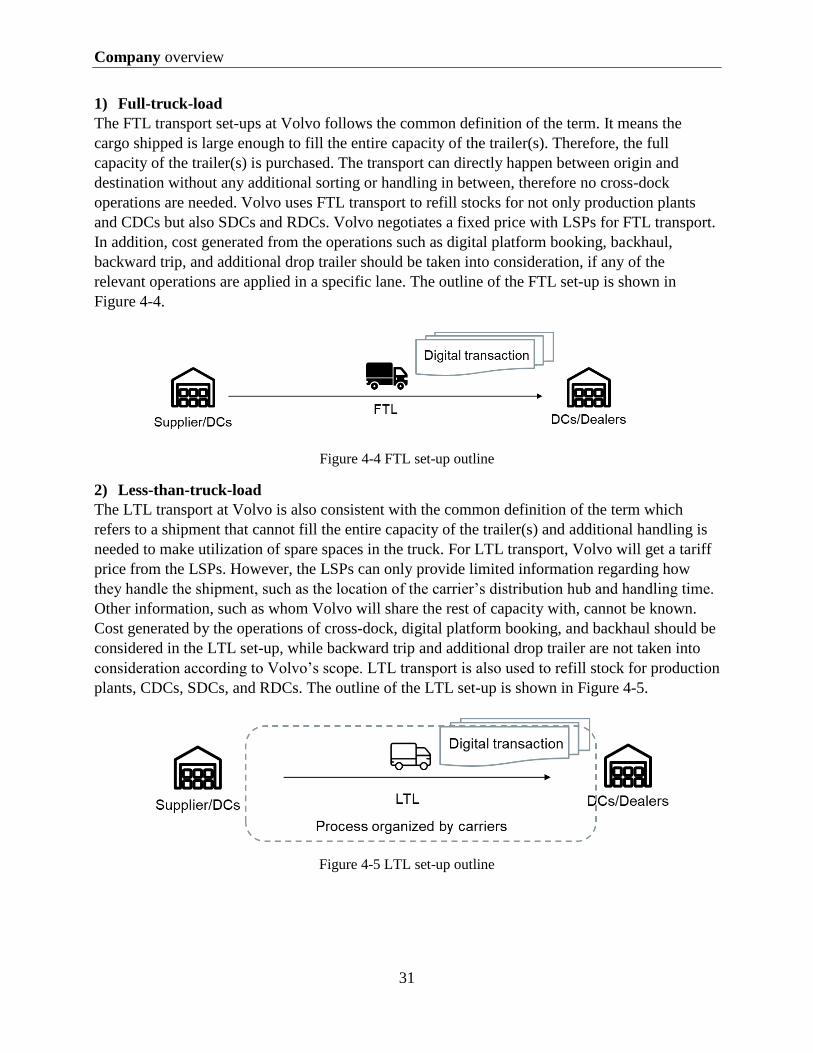
Company overview
31
1) Full-truck-load
The FTL transport set-ups at Volvo follows the common definition of the term. It means the
cargo shipped is large enough to fill the entire capacity of the trailer(s). Therefore, the full
capacity of the trailer(s) is purchased. The transport can directly happen between origin and
destination without any additional sorting or handling in between, therefore no cross-dock
operations are needed. Volvo uses FTL transport to refill stocks for not only production plants
and CDCs but also SDCs and RDCs. Volvo negotiates a fixed price with LSPs for FTL transport.
In addition, cost generated from the operations such as digital platform booking, backhaul,
backward trip, and additional drop trailer should be taken into consideration, if any of the
relevant operations are applied in a specific lane. The outline of the FTL set-up is shown in
Figure 4-4.
Figure 4-4 FTL set-up outline
2) Less-than-truck-load
The LTL transport at Volvo is also consistent with the common definition of the term which
refers to a shipment that cannot fill the entire capacity of the trailer(s) and additional handling is
needed to make utilization of spare spaces in the truck. For LTL transport, Volvo will get a tariff
price from the LSPs. However, the LSPs can only provide limited information regarding how
they handle the shipment, such as the location of the carrier’s distribution hub and handling time.
Other information, such as whom Volvo will share the rest of capacity with, cannot be known.
Cost generated by the operations of cross-dock, digital platform booking, and backhaul should be
considered in the LTL set-up, while backward trip and additional drop trailer are not taken into
consideration according to Volvo’s scope. LTL transport is also used to refill stock for production
plants, CDCs, SDCs, and RDCs. The outline of the LTL set-up is shown in Figure 4-5.
Figure 4-5 LTL set-up outline

Company overview
32
3) Dedicated delivery service
DDS is used to ship emergency orders from DCs to dealers. The order is placed on the day before
late afternoon and will be shipped to the dealer the next morning. DDS consists of two legs. The
first leg goes from a DC to carrier’s logistics hub, while the second leg is from the carrier’s hub
to dealers. The structure of DDS is shown in Figure 4-6.
Figure 4-6 DDS set-up outline
For the first leg, Volvo normally buys a fixed capacity of a truck from the carrier, which could be
seen as an LTL transport. The second leg is a distribution fully operated by the carrier. The
Distribution vehicle will not be dedicated to Volvo, but Volvo doesn’t know whom it will share
the capacity with. DDS is featured by the special time requirements. Another feature is that
usually the two legs are operated by the same carrier and Volvo will negotiate a price unit
(usually EUR/kg) for two legs as an entirety with the carrier. However, sometimes the two legs
are operated by two different carriers and there will be two separate payments for each leg to
each carrier. Similar to the LTL set-up, cost generated by the operations of cross-dock, digital
platform booking, and backhaul should be considered in the DDS set-up, while backward trip and
additional drop trailer are not taken into consideration for DDS set-up according to Volvo’s
scope.
4) Express
Express is used to ship extra emergency orders placed by the dealers which need to be fulfilled as
soon as possible. The shipment might come from either one of the DCs or even another dealer,
depending on the availability of the item. The vehicle used in the express is normally dedicated to
Volvo, which is similar to FTL. The main difference between the Express set-up and the FTL set-
up is the vehicle type. Besides, there is no additional drop trailer for the Express set-up. Express
set-up is mostly conducted by vans or taxies (passenger vehicles), while the major vehicles used
in FTL is truck with trailer. The outline of the Express set-up is shown in Figure 4-7.

Company overview
33
Figure 4-7 Express set-up outline
5) Milk-run
At Volvo, the milk-run set-up is further divided into two types: Dynamic Loads and Same Day
Delivery. Dynamic Loads is inbound milk-run from suppliers to production plants, while Same
Day Delivery ships orders from DCs to dealers. Milk-runs are also fully outsourced to carriers.
The difference between the milk-run set-up and the leg 2 of DDS (distribution) is that in the milk-
run set-up, the crew, the vehicle, and the route are all dedicated to Volvo. That means the vehicle
will only carry Volvo’s cargo and visit Volvo’s sites during a milk-run cycle. However, this set-
up will not be included in the scope of this thesis research.

Design of calculation framework
34
5 Design of calculation framework ---------------------------------------------------------------------------------------------------------------------
In the first section of this chapter, the basic theoretical framework consisting of two sections and
20 cost elements will be designed. The calculation method for each cost element will be
presented. After that, to connect the basic framework with the transport set-ups to be calculated,
modules are introduced as an intermediate. The relation between modules and cost elements,
modules, and set-ups are introduced together with the calculation method for each module.
---------------------------------------------------------------------------------------------------------------------
5.1 Basic framework
As shown in Figure 5-1, the basic framework is composed of two sections: the road freight rate
calculation section and the transport carbon emissions section. In total, 20 cost elements are
identified and will be discussed later. 18 of them belong to the road freight rate section and 2 of
them belong to the carbon emission section.
Figure 5-1 Structure of the basic framework
5.1.1 Design of Road freight section
Based on the method of cost breakdown analysis mentioned in section 2.1 and the setting for the
transport set-ups at Volvo, a cost breakdown analysis that involves three stages is conducted to
acquire the cost elements for calculation. In total, 18 cost elements are identified in the road
freight rate section and further categorized into 5 types, as shown in Figure 5-2. In the following

Design of calculation framework
35
subsections, the calculation method for each cost element will be introduced following the
sequence to three break-down.
Figure 5-2 Cost elements in road freight rate section
5.1.1.1 First breakdown
For the first breakdown, the overall road freight rate is divided into two components: the total
cost and the profit.
1) Profit
In this thesis research and from the perspective of Volvo, profit refers to the estimated profit
figure that the LSP would want to earn from running a certain lane for Volvo. Although from the
buying company’s perspective the profit is additional costs, it is needed to have a sustainable
relation with carriers. The profit is a subject metrics, depending on the operating situation of
carriers, bargaining power of the shipper. In the estimation of freight rate, it is reasonable to use
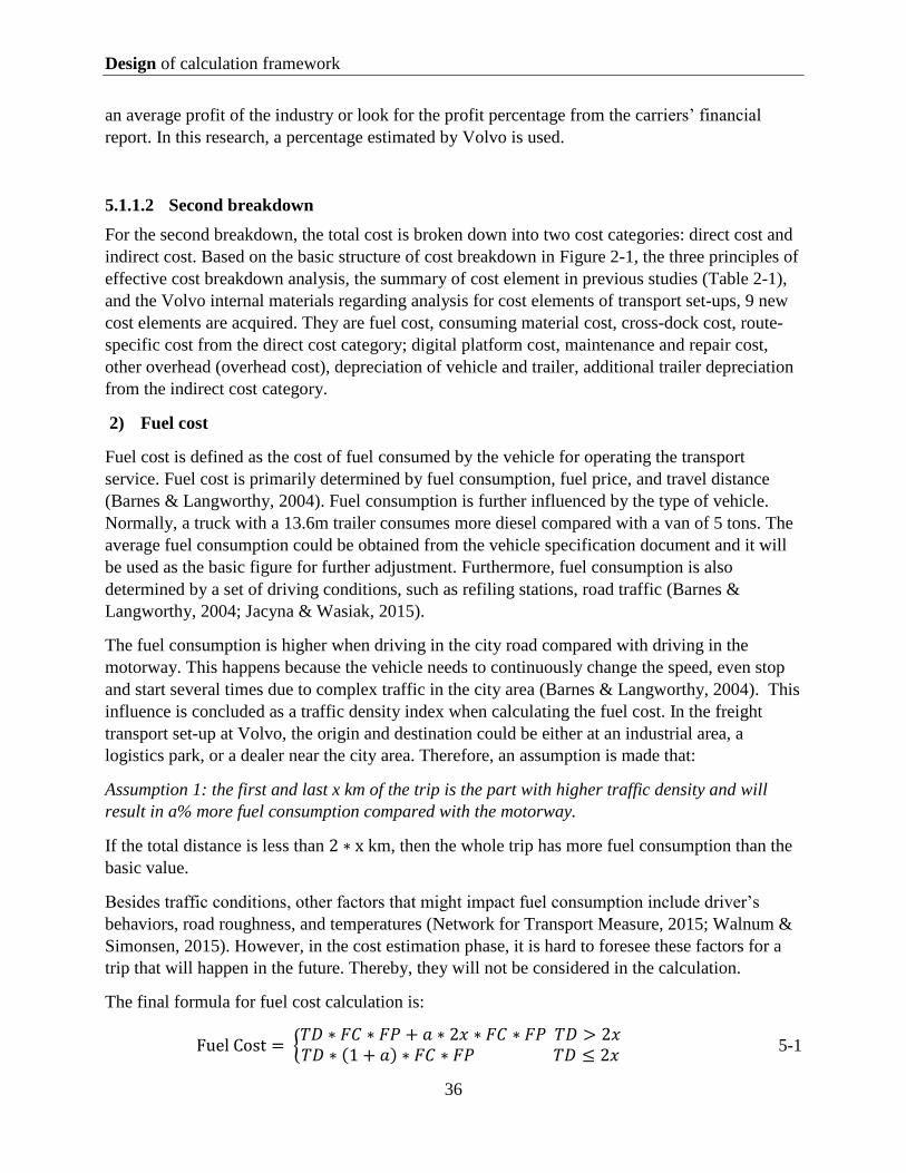
Design of calculation framework
36
an average profit of the industry or look for the profit percentage from the carriers’ financial
report. In this research, a percentage estimated by Volvo is used.
5.1.1.2 Second breakdown
For the second breakdown, the total cost is broken down into two cost categories: direct cost and
indirect cost. Based on the basic structure of cost breakdown in Figure 2-1, the three principles of
effective cost breakdown analysis, the summary of cost element in previous studies (Table 2-1),
and the Volvo internal materials regarding analysis for cost elements of transport set-ups, 9 new
cost elements are acquired. They are fuel cost, consuming material cost, cross-dock cost, route-
specific cost from the direct cost category; digital platform cost, maintenance and repair cost,
other overhead (overhead cost), depreciation of vehicle and trailer, additional trailer depreciation
from the indirect cost category.
2) Fuel cost
Fuel cost is defined as the cost of fuel consumed by the vehicle for operating the transport
service. Fuel cost is primarily determined by fuel consumption, fuel price, and travel distance
(Barnes & Langworthy, 2004). Fuel consumption is further influenced by the type of vehicle.
Normally, a truck with a 13.6m trailer consumes more diesel compared with a van of 5 tons. The
average fuel consumption could be obtained from the vehicle specification document and it will
be used as the basic figure for further adjustment. Furthermore, fuel consumption is also
determined by a set of driving conditions, such as refiling stations, road traffic (Barnes &
Langworthy, 2004; Jacyna & Wasiak, 2015).
The fuel consumption is higher when driving in the city road compared with driving in the
motorway. This happens because the vehicle needs to continuously change the speed, even stop
and start several times due to complex traffic in the city area (Barnes & Langworthy, 2004). This
influence is concluded as a traffic density index when calculating the fuel cost. In the freight
transport set-up at Volvo, the origin and destination could be either at an industrial area, a
logistics park, or a dealer near the city area. Therefore, an assumption is made that:
Assumption 1: the first and last x km of the trip is the part with higher traffic density and will
result in a% more fuel consumption compared with the motorway.
If the total distance is less than 2 ∗ x km, then the whole trip has more fuel consumption than the
basic value.
Besides traffic conditions, other factors that might impact fuel consumption include driver’s
behaviors, road roughness, and temperatures (Network for Transport Measure, 2015; Walnum &
Simonsen, 2015). However, in the cost estimation phase, it is hard to foresee these factors for a
trip that will happen in the future. Thereby, they will not be considered in the calculation.
The final formula for fuel cost calculation is:
Fuel Cost = {𝑇𝐷 ∗ 𝐹𝐶 ∗ 𝐹𝑃 + 𝑎 ∗ 2𝑥 ∗ 𝐹𝐶 ∗ 𝐹𝑃 𝑇𝐷 > 2𝑥𝑇𝐷 ∗ (1 + 𝑎) ∗ 𝐹𝐶 ∗ 𝐹𝑃 𝑇𝐷 ≤ 2𝑥
5-1

Design of calculation framework
37
(Source: Own elaboration)
TD: Trp distance (km)
FC: Fuel consumption (liter/km)
FP: Fuel price (EUR/liter)
a: Extra fuel consumption (%)
x: the distance of high − density traffic part (km)
3) Maintenance and repair cost
Maintenance and repair are categorized as one cost element, which is composed of two parts,
parts usage and labor hours. Besides, it is also impacted by other factors, such as the age of the
vehicle, the practice of the repairman, and operating conditions, together with the variety for
truck parts, increasing the difficulty in expressing the process of maintenance and repair in a
mathematical model and calculating real maintenance and repair costs (Berwick & Farooq,
2003). Another common practice in estimating maintenance and repair cost is to use an average
cost unit which is normally price per kilometer. In this framework, the latter method is adopted
and this average number is called a basic unit for maintenance and repair cost.
Both parts price and labor cost are different in different countries, which means maintenance and
repair cost is country-related. To reflect the variation among countries, the basic unit is multiplied
with a country-specific index which is calculated from the Price Level Indices (PLIs). To
implement the country index, an assumption is made:
Assumption 2: The country-specific index for maintenance and repair depends on the country of
the transport-service provider.
Country specific index
The country-specific index is obtained from Price Level Indices (PLIs) which provides a
comparison of countries’ price levels relative to the EU average (Eurostat, 2020). The PLIs are
divided into several groups, such as food and non-alcoholic beverage, clothing, electricity, and
transport services (Eurostat, 2020). Considering the topic of this research, the PLIs for transport
services are selected. The index for a country A is calculated by:
Country − specific index of country A = 𝑃𝐿𝐼𝐴
𝑃𝐿𝐼𝐶𝐵𝑈 5-2
𝑃𝐿𝐼𝐴: 𝑝𝑟𝑖𝑐𝑒 𝑙𝑒𝑣𝑒𝑙 𝑖𝑛𝑑𝑖𝑐𝑒𝑠 𝑜𝑓 𝑐𝑜𝑢𝑛𝑡𝑟𝑦 𝐴
𝑃𝐿𝐼𝐶𝐵𝑈: 𝑝𝑟𝑖𝑐𝑒 𝑙𝑒𝑣𝑒𝑙 𝑖𝑛𝑑𝑖𝑐𝑒𝑠 𝑜𝑓 𝑐𝑜𝑢𝑛𝑡𝑟𝑦 𝑓𝑜𝑟 𝑡ℎ𝑒 𝑏𝑎𝑠𝑖𝑐 𝑐𝑜𝑠𝑡 𝑢𝑛𝑖𝑡
With the above information, the formula for maintenance and repair cost is:
Maintenance and Repair Cost = CI ∗ BU ∗ TD 5-3
(Source: Own elaboration)
CI: Country index
BU: Basic cost unit (EUR/km)
TD: Trip distance (km)

Design of calculation framework
38
4) Consuming material cost
Consuming material cost is defined as the cost of different equipment related materials that are
consumed during each trip. In this thesis research, tires and lubricants are the consuming
materials that have been taken into consideration.
In the calculation process, consuming material consists of two parts, tires and lubricants, which
are both consumed by distance. The first method to calculate the consuming material cost follows
the same process as the method for maintenance and repair cost. The assumption is made that:
Assumption 3: The country-specific index for consuming material depends on the country of the
transport-service provider.
The formula is:
Consuming Material Cost = CI ∗ (TBU + LBU) ∗ TD 5-4
CI: Country − specific index
TBU: Tire basic cost unit (EUR/km)
LBU: Lubricants basic cost unit (EUR/km)
TD: Trip distance (km)
The CI (country-specific index) is calculated from formula 5-2. The consumption of tires and
lubricants is that they are less complex than the process of maintenance and repair and are more
similar to the logic of fuel consumption. Therefore, it is possible to go one step further to estimate
the cost unit in formula 5-4.
The cost of tires is impacted by vehicle type. For example, a 13.6m standard truck normally has
10 tires, while a delivery van with 1.5 tons capacity only has 4. Further, it is also impacted by the
lifetime distance. As for each tire, its lifetime depends on the road roughness, weather, and
drivers’ behaviors. Even under the same conditions, the durability of a tire will vary from brand
to brand, tire to tire. The tire company normally gives a suggested life distance. In the estimation,
an average price level and average lifetime distance of a tire from the market are adopted in the
calculation. Therefore, the tire cost could be obtained by:
Tire Cost = NoT ∗TireP
𝑇𝑖𝑟𝑒𝐿𝐷∗ 𝑇𝐷 5-5
(Source: Archondo-Callao and Faiz (1994); Berwick & Farooq (2003))
NoT: Number of tires
TireP: Tire price (EUR/tire)
TireLD: Tire lifetime distance (km)
TD: Trip distance (km)
The lubricant cost is dependent on the lubricant consumption of a certain vehicle, lubricant price,
and trip distance. There is no standard lubricant price on the market, as fuel price. However, it is
reasonable to use an average figure.
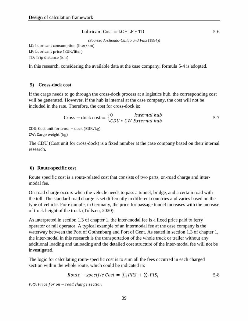
Design of calculation framework
39
Lubricant Cost = LC ∗ LP ∗ TD 5-6
(Source: Archondo-Callao and Faiz (1994))
LC: Lubricant consumption (liter/km)
LP: Lubricant price (EUR/liter)
TD: Trip distance (km)
In this research, considering the available data at the case company, formula 5-4 is adopted.
5) Cross-dock cost
If the cargo needs to go through the cross-dock process at a logistics hub, the corresponding cost
will be generated. However, if the hub is internal at the case company, the cost will not be
included in the rate. Therefore, the cost for cross-dock is:
Cross − dock cost = {0 𝐼𝑛𝑡𝑒𝑟𝑛𝑎𝑙 ℎ𝑢𝑏𝐶𝐷𝑈 ∗ 𝐶𝑊 𝐸𝑥𝑡𝑒𝑟𝑛𝑎𝑙 ℎ𝑢𝑏
5-7
CDU: Cost unit for cross − dock (EUR/kg)
CW: Cargo weight (kg)
The CDU (Cost unit for cross-dock) is a fixed number at the case company based on their internal
research.
6) Route-specific cost
Route specific cost is a route-related cost that consists of two parts, on-road charge and inter-
modal fee.
On-road charge occurs when the vehicle needs to pass a tunnel, bridge, and a certain road with
the toll. The standard road charge is set differently in different countries and varies based on the
type of vehicle. For example, in Germany, the price for passage tunnel increases with the increase
of truck height of the truck (Tolls.eu, 2020).
As interpreted in section 1.3 of chapter 1, the inter-modal fee is a fixed price paid to ferry
operator or rail operator. A typical example of an intermodal fee at the case company is the
waterway between the Port of Gothenburg and Port of Gent. As stated in section 1.3 of chapter 1,
the inter-modal in this research is the transportation of the whole truck or trailer without any
additional loading and unloading and the detailed cost structure of the inter-modal fee will not be
investigated.
The logic for calculating route-specific cost is to sum all the fees occurred in each charged
section within the whole route, which could be indicated in:
𝑅𝑜𝑢𝑡𝑒 − 𝑠𝑝𝑒𝑐𝑖𝑓𝑖𝑐 𝐶𝑜𝑠𝑡 = ∑ 𝑃𝑅𝑆𝑖𝑖 + ∑ 𝑃𝐼𝑆𝑗𝑗 5-8
𝑃𝑅𝑆: 𝑃𝑟𝑖𝑐𝑒 𝑓𝑜𝑟 𝑜𝑛 − 𝑟𝑜𝑎𝑑 𝑐ℎ𝑎𝑟𝑔𝑒 𝑠𝑒𝑐𝑡𝑖𝑜𝑛

Design of calculation framework
40
𝑃𝐼𝑆: 𝑃𝑟𝑖𝑐𝑒 𝑓𝑜𝑟 𝑖𝑛𝑡𝑒𝑟 − 𝑚𝑜𝑑𝑎𝑙 𝑓𝑒𝑒 𝑠𝑒𝑐𝑡𝑖𝑜𝑛
Although formula 5-8 shows the calculation logic, it is rather difficult to use because this requires
large manual work to check the charged sections along the route and look for the corresponding
prices. It becomes even more difficult when the route is not domestic because different countries
have different standards for toll charges. Therefore, another practical method to get real-time
route-specific costs is to connect with external databases, such as commercial toll engines.
7) Digital platform cost
Digital platform cost is the fee paid to the platform where the transaction between shipper and
carrier happens. The traditional way of transactions is through e-mail, thus the digital platform
cost will be zero. At the case company, it is common now the transaction happens in a third-party
platform and there will be a fixed cost for it.
Digital platform cost = {0 𝐸 − 𝑚𝑎𝑖𝑙𝑋 𝑇ℎ𝑟𝑖𝑑 − 𝑝𝑎𝑟𝑡𝑦 𝑝𝑙𝑎𝑡𝑓𝑜𝑟𝑚
5-9
(Source: Own elaboration)
8) Other overhead
Other overhead (overhead cost) is also a kind of indirect cost including advertising, office
equipment, and other elements (Berwick & Farooq, 2003). Overhead consists of not only the part
that cannot be attributable to specific units of output, i.e. fixed cost, but also some parts that can
be seen as variable costs (Casavant, 1993). In this research, the overhead is seen as a cost on the
top of other costs, which could be calculated by:
Other Overhead = OP ∗ (FC + LC + RSC + MRC + CMC + DC + TC + GC + IC + GC + CC) 5-10
OP: Percentage of other overhead
FC: Fuel cost (EUR)
LC: Labor cost (EUR)
RSC: Route specific cost (EUR)
MRC: Maintenance and repair cost (EUR)
CMC: Consuming material cost (EUR)
DC: Depreciation cost (EUR)
TC: Tax cost (EUR)
GC: Garage cost (EUR)
IC: Insurance cost (EUR)
CC: Cost of capital (EUR)
The cost elements mentioned in 5-10 will all be calculated in the following sections.
9) Depreciation of vehicle and trailer (Depreciation cost)

Design of calculation framework
41
The depreciation cost is calculated for both trucks and trailers if the equipment for transport
includes a trailer.
Truck Depreciation
In reality, the value of a vehicle depreciates with both mileage and age (Butler Jr, 1983; Ross,
1960). However, it is common that only one of them is considered when estimating vehicle
operating costs as long as the whole value during usage is properly divided by the time or
distance (Barnes & Langworthy, 2004; Berwick & Farooq, 2003; Sternad, 2019). In this
calculation framework, the depreciation cost of the truck is calculated based on mileage, which
means it is categorized as a variable cost. The reason is that the vehicle in the estimation is in the
high-intensity of use, thus the depreciation caused by wear and tear will be dominant.
Some research figures that the depreciation process is not a straight line over the lifetime period.
Instead, it is a concave curve with a higher rate at first and a lower rate later (Electrification
Coalition, 2010). However, in the cost estimation phase, it is hard to predict the age or used
mileage for the vehicle that is going to run the trip. Some studies also treat the depreciation rate
as constant (Jacyna & Wasiak, 2015; Sternad, 2019). In this research, this assumption is kept that:
Assumption 4: The depreciation of a vehicle is line-based, i.e. the depreciation rate is constant.
The salvage value of the vehicle is also critical in calculating the depreciation cost since it will
determine the value of the vehicle during the usage period. A vehicle normally has a suggested
lifetime distance. If the driven distance has exceeded the lifetime distance, the vehicle should be
scrapped. If a vehicle has run out of the lifetime distance, it still has a salvage value for recycling.
For transport-service providers, normally they will not use up all the lifetime distance. Instead,
they will run a car for a certain number of years and sells it in the second-hand market. An
assumption is made that:
Assumption 5: The selling value of a vehicle depends on the left distance for driving and the
minimum will the salvage value when all lifetime distance is used up.
With assumption 4 and assumption 5, the selling value for a vehicle is:
Selling Value of Vehicle (SVV) = VkI ∗ (VLD−AM∗VRY
VLD+ VSVP) 5-11
Further, the depreciation cost of the vehicle could be calculated by the following formula:
Depreciation Cost of Vehicle = VkI− SVV
AM∗VRY∗ TD 5-12
The final formula is obtained by joining equations 5-11 and 5-12 .
Depreciation Cost of Vehicle = VkI ∗ (1
VLD−
𝑉𝑆𝑉𝑃
𝐴𝑀∗𝑉𝑅𝑇) ∗ TD 5-13
VkI: Vehicle investment (EUR)
VLD: Vehicle lifetime distance (km)
VSVP: Vehicle salvage value percentage when all the distance has used up
AM: Annual mileage (km)

Design of calculation framework
42
VRY: Running time of the vehicle for transport operator(days/year)
TD: Trip distance (km)
AM (Annual mileage) is the distance that a vehicle can drive per year, which is calculated from
formula 5-14:
Annual Mileage = TPD ∗ TD ∗ 2 5-14
TPD: Trips per day
TD: Trip distance (km)
In the formula above, TPD (Trips per day) is calculated from the formula 5-21 with the
corresponding assumptions.
Trailer Depreciation
If a trailer is used in the transport, the depreciation for the trailer should also be included and it
follows the same calculation logic and vehicle. Therefore, the equation is:
Depreciation Cost of Trailer (DCT) = TrI ∗ (1
TLD−
𝑇𝑆𝑉𝑃
𝐴𝑀∗𝑇𝑅𝑇) ∗ TD 5-15
(Source: Own elaboration)
TrI: Trailer investment (EUR)
TLD: Trailer lifetime distance (km)
TSVP: Trailer Salvage value percentage when all the distance has used up
AM: Annual mileage (km)
TRT: Running time of the trailer for transport operator(year)
TD: Trip distance (km)
Depreciation Cost
With results from equation 5-13 and 5-15, the depreciation cost is:
Depreciation Cost of Trailer = DCV + DCT 5-16
DCV: Depreciation cost for the vehicle (EUR)
DCT: Depreciation cost for the trailer (EUR)
10) Additional trailer depreciation
Besides ordinary depreciation, the trailer has another part of depreciation cost which occurs when
the trailer stands for waiting during custom, intermodal, and drop trailer process. Although in
these processes, the trailer doesn’t move with the truck, it still has depreciation related to how
many days it stands. The formula is:
Additional trailer depreciation cost = 𝑇𝑟𝐼
𝑇𝑟𝐵𝐷∗𝑇𝑟𝑂𝑌∗ (DRT + CD + IMT) 5-17
TrI: Trailer investment (EUR)
TrBD: Trailer business days per year (days)

Design of calculation framework
43
TrOY: Trailer owning years (years)
DRT: Drop trailer time (days) (both drop trailer time at both destination and origin)
CD: Custome time (days)
IMT: Inter − modal time (days)
5.1.1.3 Third breakdown
According to the demand of Volvo that the waiting and handling cost, which refers to the total
cost generated by the garage, tax, labor cost, cost of capital and insurance during the waiting and
handing time, should be calculated separately as an individual cost element, those five cost
elements of garage, tax, labor cost, cost of capital and insurance need to be broken down for a
further step. Besides, backhaul cost and the backward trip cost for a round trip should also be
considered, which are the costs that take all the relevant cost elements into account during the
process of backhaul or backward trip. Thus, the third breakdown is formed.
For the third breakdown, the cost elements of waiting and handling cost, backhaul cost, and
backward trip cost are formed, along with the newly broken-down cost elements of labor cost, tax
for vehicle and trailer, garage, insurance for vehicle and trailer, and cost of capital, which have
separated their portions of the handling and waiting time.
11) Labor cost
The labor cost in this research only refers to the payment for the vehicle drivers. No labor cost for
other personnel is considered. Besides, two points should be noticed before the calculation. The
labor cost calculated in this section is the cost during driving time. The labor cost occurs in
waiting and handling is categorized in waiting and handling cost. What’s more, the labor cost
here is only the cost from the origin to destination (one-way). The labor cost that happens in
backhaul is categorized in backhaul cost.
Yearly Gross Income and Daily Compensation
Labor cost is calculated based on an hourly rate. The cost of a driver consists of four parts: basic
salary, overtime payment, bonus, and travel allowance. Basic salary, overtime payment, and
bonus form the gross income for a driver. Travel allowance is set to cover the daily expense
during the trip, including meals and accommodation (Comité National Routier, 2018). Both gross
income and travel allowance are subject to countries. A driver from France normally gets more
gross income compared with a driver from the Czech Republic. In this calculation, an assumption
is made that:
Assumption 6: the gross income of the driver depends on the country of the transport service
provider
Travel allowance is related to the living expense of each country. The allowance for a trip is set
based on the countries that this route goes through. If the driver needs to spend one day in France,
the allowance for this day should meet the living standard in France, even though the driver and
transport company both come from the Czech Republic (Comité National Routier, 2018).
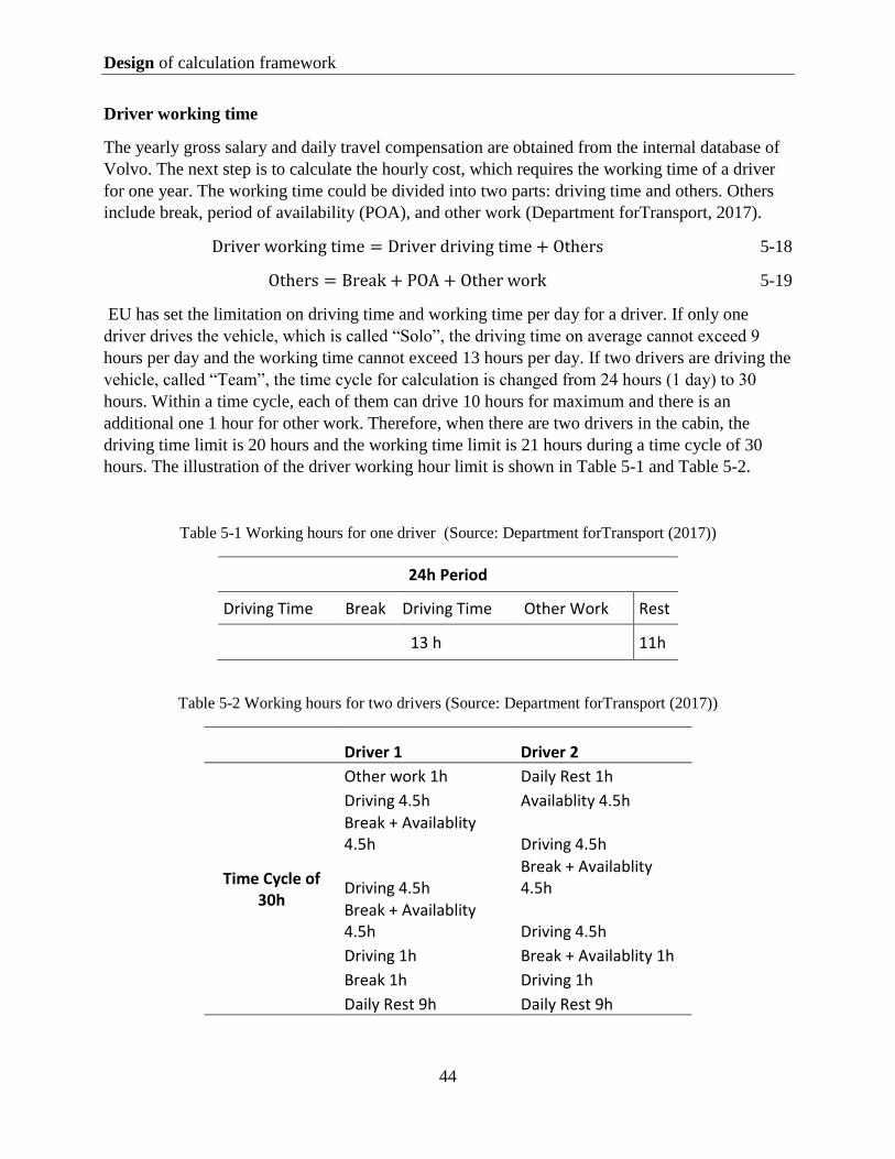
Design of calculation framework
44
Driver working time
The yearly gross salary and daily travel compensation are obtained from the internal database of
Volvo. The next step is to calculate the hourly cost, which requires the working time of a driver
for one year. The working time could be divided into two parts: driving time and others. Others
include break, period of availability (POA), and other work (Department forTransport, 2017).
Driver working time = Driver driving time + Others 5-18
Others = Break + POA + Other work 5-19
EU has set the limitation on driving time and working time per day for a driver. If only one
driver drives the vehicle, which is called “Solo”, the driving time on average cannot exceed 9
hours per day and the working time cannot exceed 13 hours per day. If two drivers are driving the
vehicle, called “Team”, the time cycle for calculation is changed from 24 hours (1 day) to 30
hours. Within a time cycle, each of them can drive 10 hours for maximum and there is an
additional one 1 hour for other work. Therefore, when there are two drivers in the cabin, the
driving time limit is 20 hours and the working time limit is 21 hours during a time cycle of 30
hours. The illustration of the driver working hour limit is shown in Table 5-1 and Table 5-2.
Table 5-1 Working hours for one driver (Source: Department forTransport (2017))
24h Period
Driving Time Break Driving Time Other Work Rest
13 h 11h
Table 5-2 Working hours for two drivers (Source: Department forTransport (2017))
Driver 1 Driver 2
Time Cycle of 30h
Other work 1h Daily Rest 1h
Driving 4.5h Availablity 4.5h
Break + Availablity 4.5h Driving 4.5h
Driving 4.5h Break + Availablity 4.5h
Break + Availablity 4.5h Driving 4.5h
Driving 1h Break + Availablity 1h
Break 1h Driving 1h
Daily Rest 9h Daily Rest 9h

Design of calculation framework
45
To calculate the actual working time of the driver, two assumptions are made:
Assumption 7: The vehicle only runs this route for the whole year and there is no limit on the
number of trips per year.
Assumption 8: The vehicle goes from the origin with cargo and returns in empty, and there will
be no stop in the back trip. The whole process is called one trip.
With two assumptions above, the working hours for a driver per day can be obtained by:
Driver working hours per day = Trips per day ∗ Duration of one trip 5-20
Where:
Trips per day = 1 (𝑇𝐷∗2
𝐴𝑣𝑒𝑆
𝐷𝑇𝐿+
𝐻𝑊𝑇
𝑊𝑇𝐿)⁄ 5-21
Duration of one trip =𝑇𝑃∗2
𝐴𝑣𝑒𝑆+ 𝐻𝑊𝑇 5-22
TD: Trip distance (km)
AveS: Average speed (km/h)
DTL: Driving time limit (hours); in the EU, it is 9 hours per day
HWT: Handling and waiting time (hours)
WTL: Working time limit (hours); in the EU, it is 13 hours per day
Then the working hours per year is calculated with the formula:
Driver working hours per year = DWHD ∗ DWDY 5-23
DWHD: Driver working hours per day (hours/day)
DWDY: Driver working days per year (days/year)
Average Speed
In formula 5-21 and 5-22, an important input is an average speed of this trip which will also
appear in formulas in the following sections. Average speed is used to calculate the driving time
of this trip. Many factors could influence the average speed. The first one is the speed limit
regulation, which is set differently in different countries. In Italy, for a vehicle over 12 tons, the
maximum speed in the urban area is 50km/h and 80 km/h on the motorway, while in Sweden, the
maximum speed is 90km/h on the motorway (European Commission, 2020). Besides policies
speed limit, other factors could also impact the average speed in real operations, such as traffic
conditions, accidents. However, in this estimating framework, it is reasonable to ignore these
arbitrary factors and focus on the influence of the speed limit.
Team index
It has mentioned in the calculation above that sometimes there could be two drivers driving in
turns for one trip. However, according to a conversation with Volvo’s employee, the transport
company will not pay double salaries in this case. Instead, the payment is a bit lower than the
doubled figure, which is indicated as the team index in the calculation. In this research, the ratio

Design of calculation framework
46
between the output of two drivers and one drive is used as the value for the team index. The
formula is:
Team index =
𝐷𝑊𝐻𝑇
𝑊𝑇𝐿𝑇𝐷𝑊𝐻𝑆
𝑊𝑇𝐿𝑆
⁄ 5-24
DWHT: Driver working hours (Team) (hours/day)
WTLT: Working time limit (Team); in the EU, it is 21 hours per day
DWHS: Driver working hours (Solo) (hours/day)
WTLS: Working time limit (Solo); in the EU, it is 13 hours per day
In this formula, DWHT and DWHS are calculated from formula 5-20, 5-21, and 5-22, with the
different driving time limits and working limit corresponding to Solo and Team.
HAZMAT and night work
HAZMAT refers to any substance that could cause harm to people, property, and the
environment (Yilmaz, Serpil, & Aplak, 2016). Most member states of the EU follow the
European Agreement concerning the International Carriage of Dangerous Goods by Road (ADR),
which requires the driver to take basic training and get a certificate to be applicable in handling
HAZMAT goods (European Commission, 2008). Therefore, the driver for a shipment with
HAZMAT is more costly than an ordinary driver, which is indicated as a HAZMAT index in the
calculation.
Night work will negatively influence the health of drivers and raise the risk of accidents.
Therefore, drivers should be compensated for driving at night (European Commission, 2002). In
this thesis, the extra cost resulting from night work is indicated as night premium factor.
Hourly rate and labor cost
With the results from the calculations above, the hourly rate of a driver could be calculated by the
following formula:
Labor Hourly Rate (LHR) = 𝐺𝐼
𝐷𝑊𝐻𝑌+
𝐷𝐶
𝐷𝑊𝐻𝐷 5-25
GI: Yealy gross income (EUR/year)
DWHY: Driver working hours per year (hours/year)
DC: Daily compensation (EUR/day)
DWHD: Driver working hours per day (hours/day)
Labor cost = LHR ×𝑇𝐷
𝐴𝑣𝑒𝑆 5-26
TD: Trip distance (km)
LHR: Labor hourly rate (EUR/h)
AveS: Average speed (km/h)

Design of calculation framework
47
Where DWHY (Driver working hours per year) is calculated from formula 5-23 and DWHD
(Driver working hours per day) is calculated from formula 5-20, 5-21, and 5-22.
12) Tax for vehicle and trailer
The tax cost calculated in this section is the cost during the driving time, while the part occurs
during the waiting and handling time will be included in waiting and handling cost.
The yearly tax differs among different vehicle types. In some countries, such as the Netherlands
and Finland, the lorry with more axles and more weight will be charged more in tax. What’s
more, the tax also varies from country to country since different countries are applying different
tax calculation system (European Commission, 2020). Then the tax cost for one trip could be
calculated by first dividing the yearly tax with the yearly working hours to get the hourly rate,
then timing the traveling time of this trip. The formula is written as:
Hourly Rate of Tax Cost (HRTC) =YT
DWHD∗VRT 5-27
Tax Cost = HRTC ∗TD
AveS 5-28
YT: Yearly tax (EUR)
DWHD: Driver working hours per day (hours/day)
VRT: Running time of the vehicle for transport operator(days/year)
HRTC: Hourly rate of tax cost (EUR/h)
TD: Trip distance (km)
AveS: Average speed (km/h)
In the formula above, DWHD (driver working hours per day) could be obtained with formula
5-20, 5-21, and 5-22.
13) Garage cost
Garage cost refers to the price that the vehicle operator needs to pay to use the garage facility
(Casavant, 1993). The calculation of garage cost follows a similar logic as tax cost. This section
only calculates the garage cost during the driving time and the cost occurs in waiting and
handling time is categorized in waiting and handling time.
Hourly Rate of Garage Cost (HRGC) = YG
DWH∗VRT 5-29
Garage Cost = 𝐻𝑅𝐺𝐶 ∗TD
AveS 5-30
YG: Yearly garage cost (EUR)
DWH: Driver working hours per day (hours/day)
VRT: Running time of the vehicle for transport operator(days/year)
HRGC: Hourly rate of garage cost (EUR/h)

Design of calculation framework
48
TD: Trip distance (km)
AveS: Average speed (km/h)
In the formula above, DWH (driver working hours per day) could be obtained with formula 5-20,
5-21, and 5-22.
14) Insurance for vehicle and trailer
In the EU, all motor vehicles must be covered by third party insurance to cover the loss caused by
accidents (European Parliament, Council of the European Union, 2009). Insurance cost
calculation follows a similar logic as tax cost. The insurance cost obtained in this section is also
the cost during the driving time, while the cost occurs during the waiting and handling time will
be involved in the waiting and handling cost.
Hourly Rate of Insurance Cost (HRIC) = YI
DWHD∗VRT 5-31
Insurance Cost = 𝐻𝑅𝐼𝐶 ∗TD
AveS 5-32
YI: Yearly Insurance (EUR)
DWHD: Driver working hours per day (hours/day)
VRT: Running time of the vehicle for transport operator(days/year)
HRIC: Hourly rate of insurance cost (EUR/h)
TD: Trip distance (km)
AveS: Average speed (km/h)
In the formula above, DWH (driver working hours per day) could be obtained with formula 5-20,
5-21, and 5-22.
15) Cost of capital
Cost of capital is a type of fixed cost which results from two sources, vehicle ownership, and
payment terms. The cost of capital caused by vehicle ownership is understood as either
opportunity cost or expected return of long-term investment during a certain period, while the
cost of capital generated by payment terms is either opportunity cost or expected return for
transport-service provider paying for clients during the negotiated period (Casavant, 1993).
Therefore, the calculation of the cost of capital could be seen as the reverse calculation of the
Accounting Rate of Return (ARR) which is the expected rate of return for a certain investment.
This relationship could be expressed as:
ARR = 𝐴𝑃
𝐴𝐼∗ 100% 5-33
Source: (Erickson, 2013; Velnampy, 2005)
Overall Cost of Capital (AP) = AI ∗ CCP(ARR) 5-34
Source: (Berwick & Farooq, 2003)

Design of calculation framework
49
AP: Average profit(EUR)
AI: Average investment (EUR)
CCP: Cost of capital percentage
In the calculation, the term “cost of capital percentage” in formula 5-34 is used to indicate the
expected return rate of investment and is the same as ARR in formula 5-33. Same as tax,
insurance, and garage cost, only the cost occurs during driving time is calculated in this section.
Cost of capital from ownership
The transport-service provider could have two options in owning a vehicle, buying, or leasing for
a certain period (Berwick & Farooq, 2003). The carrier could apply either one of them or a mixed
strategy. In the calculation, an assumption is made that:
Assumption 9: The transport-service provider owns the vehicle by purchasing.
The average investment consists of two parts, initial investment and salvage value. Salvage value
is accounted as part of average investment because this is the part of the value that could be made
in resale at any time but is held during this period (Erickson, 2013) . Therefore, the cost of capital
resulted from vehicle ownership is calculated by:
Hourly Rate of Cost of Capital from Vehicle Ownership = 𝑉𝐼+𝑉𝑆𝑉
2∗𝐶𝐶𝑃
𝑉𝑅𝑇∗𝐷𝑊𝐻𝐷 5-35
Cost of Capital from Vehicle Ownership = 𝐻𝑅𝐶𝐶𝑉 ∗𝑇𝐷
𝐴𝑣𝑒𝑆 5-36
Source: (Erickson, 2013)
VI: Vehicle investment (EUR)
VSV: Vehicle salvage value (EUR)
CCP: Cost of capital percentage
DWHD: Driver working hours per day (hours/day)
VRT: Running time of the vehicle for transport operator(days/year)
𝐻𝑅𝐶𝐶𝑉: Hourly rate of the cost of capital from vehicle ownership (EUR/h)
TD: Trip distance (km)
AveS: Average speed (km/h)
In the formula above, DWHD (driver working hours per day) could be obtained with formula
5-20, 5-21, and 5-22.
Cost of capital from payment terms
There are three types of payment terms, advance payment, cash payment, and credit payment
(Velnampy, 2005). In this calculation, credit payment, which is a permissible day in payment, is
focused as it causes capital cost for the transport service provider. The delay is negotiated by the
purchasing company and service provider. To simplify the calculation, an assumption is made
that:
Assumption 8: A year has 360 days when calculating the cost of capital generated from payment
terms.

Design of calculation framework
50
Taking payment term of 90 days as an example and a simplified cash flow of transport-service
provider could be visualized as:
Figure 5-3 Illustration of payment terms
From Figure 5-3, it could be understood that the transport-service provider holds the variable
costs of 90 days for one year (360 days), which is the annual cost of capital cost by payment
terms. Four types of variable costs are included, labor cost, fuel cost, maintenance and repair
cost, and consuming material cost. Therefore, the cost of capital caused by the credit payment
term is calculated as:
Hourly Rate of Cost of Capital from Payment Terms = 𝐴𝐹𝐶+𝐴𝐿𝐶+𝐴𝑀𝑅𝐶+𝐴𝐶𝑀𝐶
360𝑃𝑇𝐷⁄
∗1
𝑉𝑅𝑇∗𝐷𝑊𝐻𝐷∗ 𝐶𝐶𝑃 5-37
Cost of Capital from Payment Terms = 𝐻𝑅𝐶𝐶𝑃𝑇 ∗𝑇𝐷
𝐴𝑣𝑒𝑆 5-38
AFC: Annual fuel cost (EUR)
ALC: Annual labor cost (EUR)
AMRC: Annual maintenance and repair cost (EUR)
ACMC: Annual consuming cost (EUR)
PTD: Payment term days (day)
DWHD: Driver working hours per day (hours/day)
VRT: Running time of the vehicle for transport operator(days/year)
CCP: Cost of capital percentage
HRCCPT: Hourly Rate of Cost of Capital from Payment Terms (ERU/h)
TD: Trip distance (km)
AveS: Average speed (km/h)
Where:
Annual Fuel Cost = AM ∗ FC ∗ FP 5-39
Annual Labor Cost = GI + DC ∗ DWDY 5-40
Annual Maintenance and Repair Cost = AM ∗ CI ∗ MRBU 5-41
Annual Consuming Material Cost = AM ∗ CI ∗ (TBU + LBU) 5-42
AM: Annual mileage (km)
FC: Fuel consumption (l/km)
FP: Fuel price (EUR/liter)
GI: Yealy gross income (EUR/year)

Design of calculation framework
51
DWDY: Driver working hours per year (hours/year)
DC: Daily compensation (EUR/day)
CI: Country − specific index
MRBU: Maintenance and repair basic cost unit (EUR/km)
TBU: Tire basic cost unit (EUR/km)
LBU: Lubricant basic cost unit (EUR/km)
AM (Annual mileage) can be calculated with formula 5-14 in the section of depreciation cost.
With the results from formula 5-36 and 5-38, the cost of capital is obtained by:
Cost of Capital = CCPVO + CCPPT 5-43
CCPVO: Cost of capital from vehicle ownership (EUR)
CCPPT: Cost of capital from payment terms (EUR)
16) Handling and waiting cost
Handling and waiting cost occurs during the loading and unloading process to collect and deliver
cargo at stops along the route. During the loading and unloading process, the vehicle stands still,
thus the distance-based cost would not be generated, such as fuel cost, consuming material cost.
The time-related cost occurs during waiting and handling time, including labor cost, tax cost,
insurance cost, garage cost, cost of capital. The hourly rate for those cost elements has been got
from previous sections. Another factor to obtain handling and waiting cost is handling and
waiting time, which is determined by the no of stops and average waiting time at each stop.
Therefore, the handling and waiting cost could be calculated by:
Handling and waiting cost = (LHR + THR + IHR + GHR + CCPVOHR + CCPPTHR) ∗ (NoS ∗ AHWT) 5-44
LHR: Hourly rate of labor cost(EUR/h)
THR: Hourly rate of tax cost(EUR/h)
IHR: Hourly rate of insurance cost(EUR/h)
GHR: Hourly rate of garage cost(EUR/h)
CCPVOHR: Rourly rate of the cost of capital from vehicle ownership (EUR/h)
CCPPTHR: Rourly rate of the cost of capital from payment terms (EUR/h)
NoS: Number of stops (include origin and destination)
AHWT: Average handling and waiting time at each stop (h)
In the formula, LHR, THR, IHR, CCPVOHR, and CCPPTHR can be calculated from
formula5-25, 5-27, 5-29, 5-31, 5-35, and 5-38 respectively.
17) Backhaul cost
Backhaul is to haul a shipment or empty load over part of the route it has traveled from (Reichert
& Vachal, 2000; Fekpe, Alam, Foody, & Gopalakrishna, 2002). Cooper et al., (2008) has
discussed four methods in dealing with the cost generated by the backhaul trip. In this research,

Design of calculation framework
52
the second method is applied which is to assume a backhaul factor as the percentage of the cost in
the front-trip.
The backhaul factor between origin and destination depends on the relative cargo flow of the two
countries. If the destination is a ‘net producer country’ which means the flow out is larger than
the flow out, there will larger opportunity to organize a backhaul trip with a higher filling degree
(Mentzer, 1986). Therefore, the backhaul factor will be lower in this case. Therefore, the
backhaul cost is calculated by multiplying the backhaul factor with the cost of front-trip:
Backhaul Cost = BP ∗ (FC + LC + RSC + MRC + CMC + DC + TC + GC + IC + GC + CC + OC) 5-45
Source: (Cooper, Woods, & Lee, 2008)
BP: Backhaul percentage
FC: Fuel cost (EUR)
LC: Labor cost (EUR)
RSC: Route specific cost (EUR)
MRC: Maintenance and repair cost (EUR)
CMC: Consuming material cost (EUR)
DC: Depreciation cost (EUR)
TC: Tax cost (EUR)
GC: Garage cost (EUR)
IC: Insurance cost (EUR)
CC: Cost of capital (EUR)
OC: Other overhead (EUR)
18) Backward trip cost
If the trip to be calculated is a round trip which means there are cargos in the return, backward
trip cost will be applied and backhaul cost will not be included. An assumption is made for the
backward trip:
Assumption 9:The route of the backward trip is the same as the route of front-haul.
This assumption makes sure the trip distance and route-specific cost will remain the same in the
backward trip. Therefore, the backward trip cost is:
Backward trip cost = FC + LC + RSC + MRC + CMC + DC + TC + GC + IC + GC + CC + OC 5-46
FC: Fuel cost (EUR)
LC: Labor cost (EUR)
RSC: Route specific cost (EUR)
MRC: Maintenance and repair cost (EUR)
CMC: Consuming material cost (EUR)
DC: Depreciation cost (EUR)
TC: Tax cost (EUR)
GC: Garage cost (EUR)
IC: Insurance cost (EUR)

Design of calculation framework
53
CC: Cost of capital (EUR)
OC: Other overhead (EUR)
5.1.2 Design of Carbon emission section
The total carbon emissions are broken down into two elements: transport-related carbon
emissions, and cross-dock related carbon emissions, as shown in Figure 5-4.
Figure 5-4 Breakdown of carbon emissions
19) Transport carbon emissions
The carbon emissions generated during transport mainly result from fuel consumption. Besides
the difference in fuel consumption level among different vehicle types, the carbon emissions of a
vehicle could also vary from brand to brand, version to version, depending on the technology the
vehicle used. However, in this research, only the basic carbon emissions caused by fuel
consumption is considered. More advanced differences will be ignored. An assumption is made
that:
Assumption 13: All the carbon in the fuel is burned fully and converts to carbon dioxide.
The carbon emissions are determined by the fuel consumption level of the vehicle as well as the
carbon content and density of the fuel type (Network for Transport Measure, 2015). Carbon
content refers to the carbon content of the fuel as a percentage of its mass (HOMER Energy,
2014). Both carbon content and fuel density can be obtained from the public data source on fuel
information. In this research, the density of diesel is 0.832 kg/L (Engineering ToolBox, 2003),
while the carbon density of 86.2% (Ecoscore, 2020). The carbon emissions happen during
transport can be calculated by:
Transport Carbon Emissions = TD ∗ FC ∗ FD ∗ CC ∗ MWR 5-47
Source: (Network for Transport Measure, 2015)
FC: Fuel consumption (liter/km)
FD: Fuel density (kg/liter)
CC: Carbon content (%)
MWR: Molecular weight relations
TD: Trip distance (km)
In formula 5-47, MWR (Molecular weight relations) is equal to 44/12. This variable is used to
convert the weight of carbon to the weight of carbon dioxide.

Design of calculation framework
54
20) Cross-dock carbon emissions
If the route to be calculated consists of cross-dock at the logistics hub, the carbon emissions in
this process should also be included. Assessing the carbon emissions level at logistics facilities is
a complex process because the emissions level differs from the type of the facility and functions
performed in the facility (Rüdiger, Schön, & Dobers, 2016; Dobers, Ehrler, Davydenko, Rüdiger,
& Clausen, 2019). In this research, the cargo being transported needs to quickly go through the
cross-dock process at the logistics hub and be shipped to the destination within the lead time.
Therefore, the logistics hub is a transshipment terminal with a focus on the cross-dock process.
The carbon emissions from cross-dock is calculated by:
Cross − dock Carbon Emissions = CDCEU ∗ WS 5-48
Source: (Dobers, Ehrler, Davydenko, Rüdiger, & Clausen, 2019; Rüdiger, Schön, & Dobers, 2016)
CDCEU: Cross − dock carbon emissions unit (EUR/kg)
WS: Weight of the shipment (kg)
5.1.3 Summary of fact data
The data source used to estimate the cost elements in the basic framework is summarized in
Table 5-3.
Table 5-3 Source of fact data in estimating freight rate
Section Data type Example Source
Road freight rate section
Vehicle-related data Truck investment; fuel consumption…
Internal database of Volvo
Country-related data Working time Department forTransport (2017)
Gross salary, daily compensation Internal database of Volvo
Profit An estimated percentage from Volvo
Route-related data Distance, toll cost… External toll engine used by Volvo
Lane setting Single/round, drop trailer, origin, destination
Bid information of Volvo
Cross-dock cost unit Figure provided by Volvo
Booking platform cost unit
Figure provided by Volvo
Carbon emission section
Fuel consumption Volvo internal database
Fuel-related data Carbon content, fuel density Engineering ToolBox (2003) Ecoscore (2020)
Cross-dock carbon emission unit
Dobers et al., (2019) Rüdiger te al., (2016)

Design of calculation framework
55
5.2 Calculation of Modules and set-ups
5.2.1 The design of modules
Each transport set-up consists of several activities. For example, the DDS set-up includes line-
haul transport, cross-dock, and distribution. Different activities should comprise different cost
elements and be calculated in different ways. To build up the connection between the calculation
methods for cost elements and the estimation of the total rate for each transport set-up, modules
are introduced as intermediate.
The modules are derived from the activities in each transport set-up. They are designed to build
connections between transport set-ups and the basic framework. The relations are shown in
Figure 5-5. Each module includes a set of relevant cost elements, while different modules can be
combined to form a transport set-up. The division of the modules and the cost elements included
in each module are established according to the analysis of the four Volvo’s transport set-ups,
which has been introduced in section 4.3.2. As is shown in Figure 5-5, five modules are
introduced for the road freight rate section, the FTL line-haul module, the LTL line-haul module,
the Distribution module, the Cross-dock module, and the Digital platform module. Four modules
are introduced for the carbon emission section, FTL line-haul carbon emissions module, LTL
line-haul carbon emissions module, distribution carbon emissions module, and cross-dock carbon
emissions module.
Figure 5-5 Basic framework, modules, and set-ups

Design of calculation framework
56
5.2.2 Modules and set-ups in road freight rate section
5.2.2.1 Cost elements in modules
In Table 5-4, the cost elements included in each module are listed. The left column is the 18 cost
element in the road freight rate section, while the top row is the name of modules in the section.
If the cell is marked by “Y”, it means the cost element is included in the corresponding module.
For example, the FTL line-haul module includes all the cost elements, and LTL line-haul module
includes the cost elements besides additional trailer depreciation and backward cost a round trip.
Table 5-4 The modules and cost elements included
5.2.2.2 Set-ups and modules
The following figures illustrate the connection and relation between the set-ups and the modules,
i.e. how the modules are combined to form each transport set-up at the case company.

Design of calculation framework
57
FTL set-up
The FTL set-up, according to the set-up introduction mentioned in section 4.3.2 can be seen as a
combination following the sequence of an FTL line-haul module and a digital platform module,
as is shown in Figure 5-6.
Figure 5-6 FTL set-up and modules involved
Express set-up
The Express set-up is similar to the FTL set-up, with the only difference of vehicle type that is
used for the delivery, as is introduced in section 4.3.2. As a result, the Express set-up can also bee
seen as a combination following the sequence of an FTL line-haul module and a Digital platform
module.
LTL set-up:
The LTL set-up, according to set-up introduction mentioned in section 4.3.2can be seen as a
combination following the sequence of a (pick-up) Distribution module, a Cross-dock module, an
LTL line-haul module, a Cross-dock module, and a (delivery) Distribution module; plus a Digital
platform module, as is shown in Figure 5-7.
Figure 5-7 LTL set-up and modules involved
DDS set-up
The DDS set-up, according to the set-up introduction mentioned in section 4.3.2 can be seen as a
combination following the sequence of an LTL line-haul module, a Cross-dock module, and a
Distribution module; plus a Digital platform module, as is shown in Figure 5-8.

Design of calculation framework
58
Figure 5-8 DDS set-up and modules involved
The result for the road freight rate calculation of each set-up is the sum-up result of the road
freight rate calculation figure from all the corresponding modules in the set-up. In the next
section, the method of how to calculate all the cost elements within a specific module will be
illustrated.
5.2.2.3 Calculation method for each module
1) FTL line-haul module
In the FTL line-haul module, the whole vehicle is dedicated to the shipment, thus all the cost will
be allocated to the shipment. Therefore, the cost of the FTL line-haul module is the sum-up of all
the cost elements.
Cost of FTL linehaul module = FC + LC + RSC + MRC + ATD + CMC + DC + TC + GC + IC + GC + CC + OC + {𝐵𝐻𝐶𝐵𝑊𝐶
5-49
FC: Fuel cost (EUR)
LC: Labor cost (EUR)
RSC: Route specific cost (EUR)
MRC: Maintenance and repair cost (EUR)
MRC: Additional trailer depreciation cost (EUR)
CMC: Consuming material cost (EUR)
DC: Depreciation cost (EUR)
TC: Tax cost (EUR)
GC: Garage cost (EUR)
IC: Insurance cost (EUR)
CC: Cost of capital (EUR)
BHC: Backhaul cost (EUR)
BWC: Backward trip cost(EUR)
OC: Other overhead (EUR)
The cost elements in the formula are calculated from formulas in section 5.1.1. Only one of BHC
(backhaul cost) and BWC (Backward trip cost) will be applicable, depending on if it is a single
trip or round trip.
2) LTL line-haul module

Design of calculation framework
59
In LTL line-haul, the cost for the vehicle is the same as an FTL line-haul transport. However, the
shipment only accounts for a part of the whole loads so that only part of the total cost should be
allocated to the shipment. The allocation is based on the share of the shipment size to the loads in
the vehicle. The assumption is made that:
Assumption 10: The filling degree of the vehicle in LTL line-haul is 100% since the transport-
service provider will manage to fill the vehicle through cross-dock.
The size of the shipment is the chargeable weight of the shipment, which is the larger value
between the actual weight and volumetric weight. Volumetric weight is a calculation converting
the volume to weight to reflect the density of the cargo. A less dense item usually occupies more
volume of the vehicle than the weight, thus it is more reasonable to charge it by volumetric
weight rather than the actual weight (Borderlinx, 2020). The convert is done by a dim factor
which is different for different transport modes and in different regions. In the EU, the dim factor
is normally 1𝑚3 = 333kg for road freight transport (DB Schenker, 2019).
Charge Payload = Max(AC, DF ∗ VS) 5-50
AC: Actual weight (kg)
DF: Dim factor
VS: Volume of the cargo (m3)
Therefore, the cost of LTL line-haul is calculated by:
CLTLM = (FC + LC + RSC + MRC + CMC + DC + TC + GC + IC + GC + CC + OC + BHC) ∗ 𝐶𝑃
𝑉𝐶 5-51
FC: Fuel cost (EUR)
LC: Labor cost (EUR)
RSC: Route specific cost (EUR)
MRC: Maintenance and repair cost (EUR)
CMC: Consuming material cost (EUR)
DC: Depreciation cost (EUR)
TC: Tax cost (EUR)
GC: Garage cost (EUR)
IC: Insurance cost (EUR)
CC: Cost of capital (EUR)
BHC: Backhaul cost (EUR)
CP: Chargeable payload (EUR)
OC: Other overhead (EUR)
VC: Vehicle capacity (kg)
CP (chargeable payload) is calculated from formula 5-50.
3) Distribution module
The Distribution module is more complex in reality than the FTL line-haul and LTL line-haul
module, because a distribution cycle includes not only the destination of the shipment but also the
sites for other customers of the transport-service provider. The stops and loads of distribution are

Design of calculation framework
60
unknown in the cost estimating phase for both the shipper and the carrier. There are two main
changes in the cost calculation of the distribution module.
Change in variables
Two assumptions that influence the value of variables are made to make the calculation viable.
Assumption 11 The length of a distribution cycle is x km on average.
Assumption 12: The average speed of a distribution cycle is v km/h.
With assumption 11 and assumption 12, the maximum number of stops in a distribution cycle can
be calculated by:
No of stops = 𝐷𝑊𝐻𝐷−𝑥
𝑣⁄ −𝐻𝑊𝑇𝐻
𝐻𝑊𝑇𝑆 5-52
DWHD: Driver working hours per day (hour/day)
x: Trip distance of a distribution cycle(km)
v: Average speed of the distribution cycle (km/h)
HWTH: Handing and waiting time at the hub (hour)
HWTS: Handling and waiting time at each stop (hour)
The total handling and waiting time of a distribution cycle is
Handling and waiting time = NoS ∗ HWTS + HWTH 5-53
NoS: Number of stops
HWTH: Handing and waiting time at the hub (hour)
HWTS: Handling and waiting time at each stop (hour)
In the calculation of each cost element, the new values of trip distance, average speed, and
handling and waiting time should be used.
Share of the shipment
Same as the logic in the LTL line-haul module, the shipment only accounts for a proportion of
the total cost of the vehicle depending on the share of the shipment size to the loads. However, in
distribution transport, the filling degree is keeping changing. In a delivery distribution, the filling
degree normally keeps decreasing, while in a pick-up distribution, the filling degree keeps
increasing. If a distribution cycle includes both collection and delivery, the filling degree will
fluctuate. Therefore, the assumption in the LTL line-haul module will not be applicable. It is
more reasonable to assume a certain filling degree level. The relationship between vehicle
capacity, loads, and size of this shipment is shown in Figure 5-9:

Design of calculation framework
61
Figure 5-9 Relations of capacity, loads and shipment size
The cost of the distribution module is calculated by:
CMRM = (FC + LC + RSC + MRC + CMC + DC + TC + GC + IC + GC + CC + OC) ∗ 𝑆𝑆𝐹𝑆 5-54
Where
𝑆𝑆𝐹𝑆 = 𝐶𝑃
𝑉𝐶⁄
𝑉𝐹𝐷 5-55
CMRM: Cost of the distribution module (EUR)
SSFS: Share of the shipment to the loads
CP: Chargeable payload (kg)
VC: Vehicle capacity (kg)
VFD: Vehicle filling degree
FC: Fuel cost (EUR)
LC: Labor cost (EUR)
RSC: Route specific cost (EUR)
MRC: Maintenance and repair cost (EUR)
CMC: Consuming material cost (EUR)
DC: Depreciation cost (EUR)
TC: Tax cost (EUR)
GC: Garage cost (EUR)
IC: Insurance cost (EUR)
CC: Cost of capital (EUR)
OC: Other overhead (EUR)
CP (Chargeable payload) could be obtained through formula 5-50.
4) Cross-dock module
As introduced in the previous section, there is only one cost element under the cross-dock
module. Therefore, the cost of the module is:
Cost of cross − dock module = CDC 5-56
CDC: Cross − dock cost (EUR)
Cross-dock cost is calculated from formula 5-7.

Design of calculation framework
62
5) Digital platform module
Same as the cross-dock module, there is only one element within the digital platform module.
Therefore, the cost of digital platform module is
Cost of digital platform module = DPC 5-57
DPC: Digital platform cost (EUR)
DPC (Digital platform cost) is calculated from formula 5-9
5.2.3 Modules and set-ups in road freight rate section
5.2.3.1 Set-ups and modules
The module split in the carbon emissions section follows a similar method as section 5.2.2.
However, as the digital platform does not generate any carbon emissions considered in the set-up,
only four modules are split compared with the five modules in the road freight rate section. They
are the FTL line-haul carbon emissions module, LTL line-haul carbon emissions module,
Distribution carbon emissions module, and Cross-dock carbon emissions module.
Therefore, in the carbon emissions section, the FTL set-up can be seen as a single FTL line-haul
carbon emissions module. Similarly, the Express set-up can also be seen as a single FTL line-haul
carbon emissions module. The LTL set-up can be seen as a combination following the sequence
of a Distribution carbon emissions module, a Cross-dock carbon emissions module, an LTL line-
haul carbon emissions, a Cross-dock carbon emissions module, and a Distribution carbon
emissions module. The DDS set-up can be seen as a combination following the sequence of an
LTL line-haul carbon emissions module, a Cross-dock carbon emissions module, and a
Distribution carbon emissions module.
Similarly to the calculation method for the set-ups of the road freight rate section, the result for
the transport carbon emissions calculation of each set-up is the sum-up result of the emissions
figures from all the corresponding modules in the set-up. In the next section, the method of how
to calculate the carbon emissions within a specific module will be illustrated.
5.2.3.2 Calculation method for each module
1) FTL line-haul carbon emissions module
The carbon emissions in the FTL line-haul carbon emission module is only generated by
transport.
FTL line − haul carbon emissions = TCE 5-58
TCE: Transport carbon emissions (kg)
TCE is calculated from formula 5-47.

Design of calculation framework
63
2) LTL line-haul carbon emissions module
The carbon emissions generated by the vehicle during the LTL line-haul carbon emission module
should be allocated based on the share of the shipment. The assumption is still valid here.
LTL line − haul carbon emissions = TCE ∗ 𝐶𝑃
𝑉𝐶 5-59
(Source: Own elaboration)
CP: Chargeable payload (kg)
VC: Vehicle capacity (kg)
TCE: Transport carbon emissions (kg)
TCE is calculated from formula 5-47.
3) Distribution carbon emissions module
In the Distribution carbon emissions module, the carbon emissions are allocated based on the
share of the shipment size to the loads.
Milk − run carbon emissions = TCE ∗ 𝐶𝑃
𝑉𝐶⁄
𝑉𝐹𝐷 5-60
(Source: Own elaboration)
CP: Chargeable payload (kg)
VC: Vehicle capacity (kg)
VFD: Vehicle filling degree
TCE: Transport carbon emissions (kg)
4) Cross-dock carbon emissions module
In the module of cross-dock carbon emissions, there is only one element.
Cross − dock carbon emission = CDCE 5-61
CDCE: Cross − dock carbon emissions (kg)
CDCE could be obtained from formula 5-48.

Development of calculation tools
64
6 Development of calculation tools
---------------------------------------------------------------------------------------------------------------------
To apply the theoretical framework of road freight rate and carbon emissions calculation, two
different tools, which are tailored to the business context of the case company, are developed.
The first tool is developed based on Visual Basic for Applications (VBA) in Excel and is called a
“VBA-based tool”, while the second one is based on spreadsheets of Excel and is called a
“spreadsheet-based tool”. The structure and features of both tools are presented in this chapter.
---------------------------------------------------------------------------------------------------------------------
6.1 Calculation tool in VBA
6.1.1 Structure of the VBA-based tool
The structure of the VBA-based tool is shown in Figure 6-1
Figure 6-1 Structure of VBA-based tool
(Source: Own elaboration)
There are three parts in the VBA-based tool, user form, macros, and datasheets. The role of three
parts and the connections among them are presented in the following.
User Form
User form is the window where the interaction between users and the VBA-based tool happens. It
will be achieved by using the “UserForm” object in VBA. Users need to select the transport set-
up they want to calculate and input required data about the route in the user form, such as
destination and origin. The user form can present some important fact data retrieved from fact
data sheets to the user.
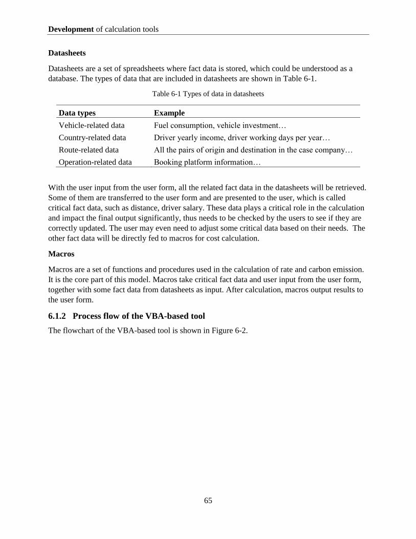
Development of calculation tools
65
Datasheets
Datasheets are a set of spreadsheets where fact data is stored, which could be understood as a
database. The types of data that are included in datasheets are shown in Table 6-1.
Table 6-1 Types of data in datasheets
Data types Example
Vehicle-related data Fuel consumption, vehicle investment…
Country-related data Driver yearly income, driver working days per year…
Route-related data All the pairs of origin and destination in the case company…
Operation-related data Booking platform information…
With the user input from the user form, all the related fact data in the datasheets will be retrieved.
Some of them are transferred to the user form and are presented to the user, which is called
critical fact data, such as distance, driver salary. These data plays a critical role in the calculation
and impact the final output significantly, thus needs to be checked by the users to see if they are
correctly updated. The user may even need to adjust some critical data based on their needs. The
other fact data will be directly fed to macros for cost calculation.
Macros
Macros are a set of functions and procedures used in the calculation of rate and carbon emission.
It is the core part of this model. Macros take critical fact data and user input from the user form,
together with some fact data from datasheets as input. After calculation, macros output results to
the user form.
6.1.2 Process flow of the VBA-based tool
The flowchart of the VBA-based tool is shown in Figure 6-2.

Development of calculation tools
66
Figure 6-2 Process flowchart of the VBA-based tool
The process flow of VBA-based tool is divided into five steps:
Step1: The user selects one of the four set-ups from the drop-down list
Step2: The user inputs all the basic information of the lane to be calculated, such as origin and
destination.
Step3: The user clicks the button “Get Data”. Then critical fact data will be retrieved from data
sheets and shown in the user form. The user can check if the data is correct and reasonable.
Step4: The user can change the fact data if needed.
Step5: The user clicks the button “Cal”. Then the results will be calculated and shown in a new
sheet.

Development of calculation tools
67
6.2 Spreadsheet-based Tool
6.2.1 Structure of spreadsheet-based tool
Unlike the VBA-based tool which integrates all five set-ups into one file, five different files, i.e.
workbooks of Excel, are created for five transport set-ups respectively, and each of them contains
a copy of all the fact data. The reason for this design is that the calculation process in the
spreadsheet takes much more space than in VBA. If all the five set-ups are put in one file, it
would cause trouble for the user in sorting out relevant information. The structure of the
spreadsheet-based tool is shown in Figure 6-3.
Figure 6-3 Structure of spreadsheet-based calculation
(Source: Own elaboration)
In the spreadsheet-based tool, the five files have a similar structure. Within one file, there are
three parts, an input and result sheet, datasheets, and calculation sheets. The function of each part
and their relations are explained in the following.
Input and Result Sheet
The input and result sheet is the sheet where the user types in all the needed information for
calculation. The results calculated from calculation sheets are transferred to this sheet and are
added together to get the final results. The idea is the user only needs to interact with this sheet,
although the most calculation happens in other sheets.
Datasheets
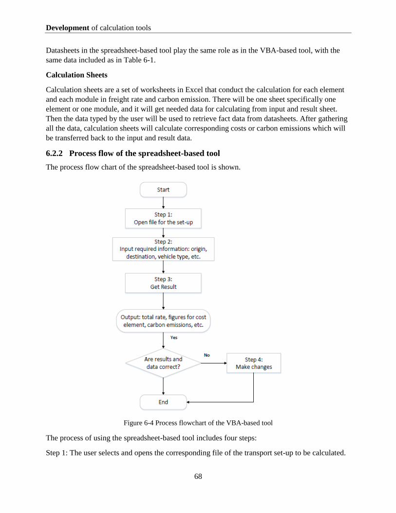
Development of calculation tools
68
Datasheets in the spreadsheet-based tool play the same role as in the VBA-based tool, with the
same data included as in Table 6-1.
Calculation Sheets
Calculation sheets are a set of worksheets in Excel that conduct the calculation for each element
and each module in freight rate and carbon emission. There will be one sheet specifically one
element or one module, and it will get needed data for calculating from input and result sheet.
Then the data typed by the user will be used to retrieve fact data from datasheets. After gathering
all the data, calculation sheets will calculate corresponding costs or carbon emissions which will
be transferred back to the input and result data.
6.2.2 Process flow of the spreadsheet-based tool
The process flow chart of the spreadsheet-based tool is shown.
Figure 6-4 Process flowchart of the VBA-based tool
The process of using the spreadsheet-based tool includes four steps:
Step 1: The user selects and opens the corresponding file of the transport set-up to be calculated.

Development of calculation tools
69
Step 2: The user types in the basic information of the lane, such as origin and destination.
Step 3: The results will be obtained and shown once all the required information is fed.
Step 4: The user can check the results and go into other sheets to change fact data if needed.
6.3 Comparison and discussion
The VBA-based tool and spreadsheet-based tool are built up with the same framework of
calculating freight rate and carbon. They also share the same fact data. However, the techniques
they are applying give them different features so that they are suitable in different environments.
The VBA-based tool is more user-friendly because the user only needs to interact with a well-
organized user form, the calculation process and data needed in between are written in macros
and invisible to the user. The interface of the VBA-based tool is closer to standard software
compared with spreadsheets, thus it can be used as a demo if further development of advanced
software is needed. However, the VBA-based tool is only applicable for lane-by-lane calculation,
which means it cannot take a batch of lanes at the same time and make the calculation.
In contrast, the spreadsheet-based tool is much less condensed compared with the VBA tool
because all the calculations and intermediate data are presented in the sheets. However, this also
provides the user with easier access to check the intermediate results of the calculation. The most
advantage of the spreadsheet-based tool is it can take a set of lane information and carry out
calculations in batches.
In conclusion, the relations and features of the two tools are illustrated in Figure 6-5.

Development of calculation tools
70
Figure 6-5 Comparison of two tools
The screenshots of the interface of both tools are demonstrated in Appendix A and screenshots of
codes are shown in Appendix B.

Test of framework analysis
71
7 Test of framework analysis ---------------------------------------------------------------------------------------------------------------------
In this chapter, several routes from the case company are selected as samples to test the
estimation framework and tool. The detailed breakdown structure of the freight rate will be
illustrated and carbon emissions generated from this transport will be shown. Besides, the
estimated freight rates, current bid prices, and estimated rates obtained from an internal tool at
the case company will be compared. Express set-up will not be included in the analysis due to
limited data. This section will only illustrate figures, more detailed comparison and discussion
will be done in Chapter 8.
---------------------------------------------------------------------------------------------------------------------
7.1 Rate structure and carbon emission
In this section, in total eight samples for three set-ups at the case company (FTL, LTL, and DDS)
will be tested. Although the calculation logic for Express is built up in chapter 4, it will not be
included in this section due to data availability. All the tested samples are summarized in the
following table.
Table 7-1 Summary of tested samples
Set-up FTL LTL DDS
Tested Samples
Sample 1 Sample 2 Sample 3 Sample 4 Sample 5 Sample 6 Sample 7 Sample 8
Lane A Lane B Average of
8 single trips Average of
2 round trips Lane C
Average of 8 lanes
Lane D Average of
8 lanes
Domestic/ International
Domestic International Mix Mix Domestic Domestic Domestic Domestic
LSP Country Sweden Czech republic Mix Mix Sweden Sweden Sweden Sweden
Shipment Weight Full truck Full truck Full truck Full truck 17505kg Mix 438.9kg Mix
7.1.1 Full-Truck-Load
Under the FTL set-up of the case company, two lanes are selected as a sample to illustrate the
rate structure of individual shipment. Then, the average rate structure of ten randomly selected
lanes is presented. The first lane, which is marked as lane A, is a domestic transport in Sweden
with a trip distance of 153km. The second lane marked as lane B is a cross-border transport
which is 411km long. Other than the difference in trip distance, origin, and destination, two lanes
are carried by different types of vehicle and lane B has a drop trailer setting at the origin, while
lane A does not. The difference between the two lanes are summarized in Table 7-2
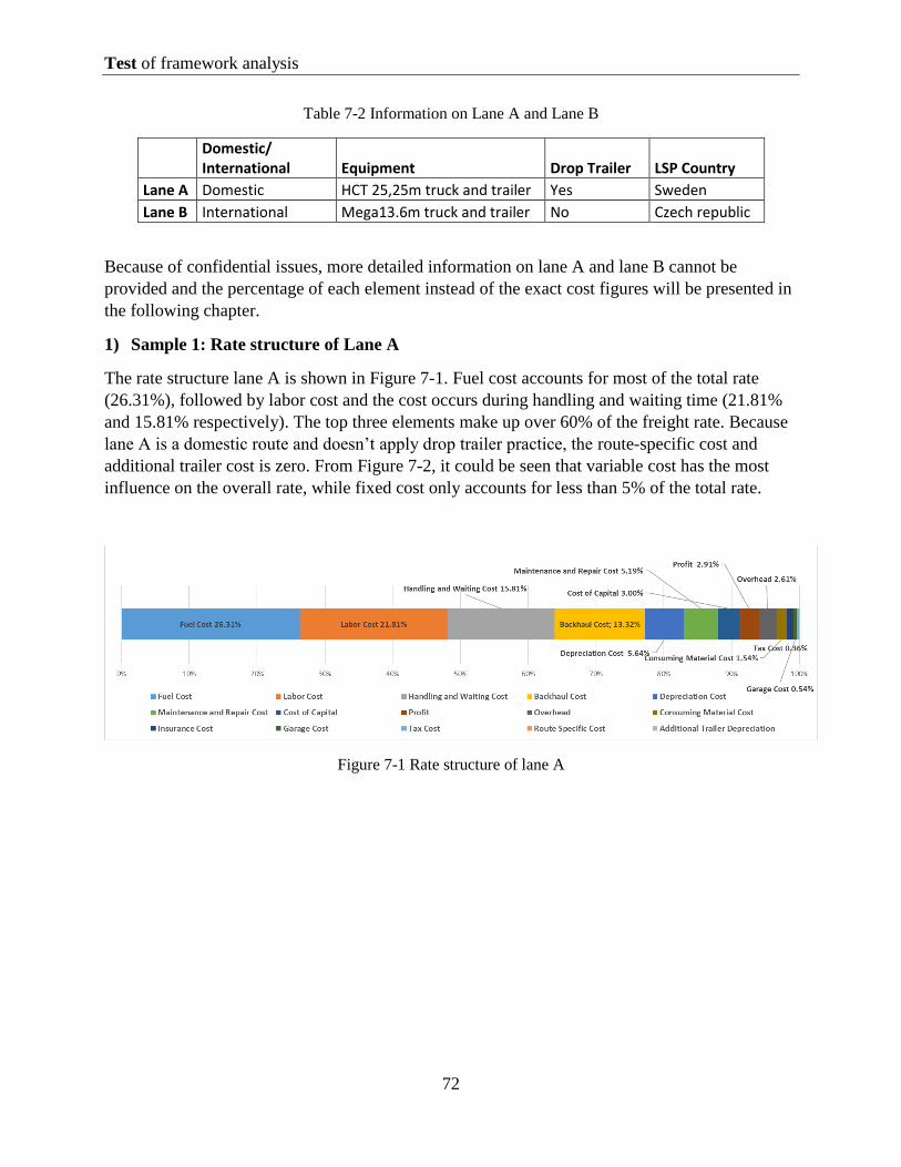
Test of framework analysis
72
Table 7-2 Information on Lane A and Lane B
Domestic/ International Equipment Drop Trailer LSP Country
Lane A Domestic HCT 25,25m truck and trailer Yes Sweden
Lane B International Mega13.6m truck and trailer No Czech republic
Because of confidential issues, more detailed information on lane A and lane B cannot be
provided and the percentage of each element instead of the exact cost figures will be presented in
the following chapter.
1) Sample 1: Rate structure of Lane A
The rate structure lane A is shown in Figure 7-1. Fuel cost accounts for most of the total rate
(26.31%), followed by labor cost and the cost occurs during handling and waiting time (21.81%
and 15.81% respectively). The top three elements make up over 60% of the freight rate. Because
lane A is a domestic route and doesn’t apply drop trailer practice, the route-specific cost and
additional trailer cost is zero. From Figure 7-2, it could be seen that variable cost has the most
influence on the overall rate, while fixed cost only accounts for less than 5% of the total rate.
Figure 7-1 Rate structure of lane A

Test of framework analysis
73
Figure 7-2 Comparison of different categories of lane A
2) Sample 2: Rate structure of lane B
The structure of lane B is shown in Figure 7-3. Same as the rate structure of lane A, fuel cost
accounts for the largest part, over 30% to the total rate. The labor cost is still the second largest
element, representing 11% of the overall rate. The third-largest share comes to route-specific cost
which is followed by additional-trailer depreciation cost. These four elements cover nearly 60%
of the total rate.
From Figure 7-4, it could be noticed that fixed cost still has much less impact on the overall cost
compared with process cost and variable cost. Variable cost is still dominant, accounting for
around 80% of the overall rate.
Figure 7-3 Rate structure of lane B

Test of framework analysis
74
Figure 7-4 Comparison of cost categories of lane B
3) Sample 3: Average rate structure of 10 lanes
The randomly selected lanes have a mix of domestic and international transport. 8 of them are
single trips, while 2 of them are round trips meaning the rates include the shipment for both
directions. The basic information of the 10 lanes is summarized in table Table 7-3.
Table 7-3 Summary of information of 10 lanes
Lane Domestic/
International Equipment
Drop
Trailer LSP Country Single/Round
1 Domestic HCT 25,25m truck and trailer Yes Sweden Single
2 International Mega 13.6m truck and trailer No Czech republic Single
3 International Mega 13.6m truck and trailer Yes Czech republic Single
4 International Mega 13.6m truck and trailer Yes Czech republic Single
5 Domestic HCT 25,25m truck and trailer No Sweden Round
6 International Standard 13.m truck and trailer No Poland Round
7 International Mega 13.6m truck and trailer No Czech republic Single
8 Domestic Mega 13.6m truck and trailer No Germany Single
9 International Standard 13.m truck and trailer No Czech republic Single
10 International Mega 13.6m truck and trailer No Slovakia Single
The analysis of the average rate structure is further divided into two groups, single trips, and
round trips. The reason is that in round trips, the backward trip cost is almost half of the total rate,
but this cost element is zero in the single trip. Therefore, the high share of backward trip costs in
the round trip settings will be distorted if they are averaged with the lanes that have a single trip
setting. The distortion will also happen to backhaul cost if the single trip setting is analyzed with
the round trip setting because there is no backhaul cost in the round trip. Figure 7-5 shows that
for single-trip lanes, the fuel cost is still the largest share to the overall rate (28.82%) followed by

Test of framework analysis
75
labor cost which accounts for 14% on average. The backhaul cost in a single trip has an obvious
influence on the total rate with a share of 9.14% on average. As for the two round trips, the
backward cost during round trip accounts for nearly 48.93% of the total rate. Expect the cost
during the backward trip, fuel cost and labor cost still rank as the first two largest cost elements,
with the proportion of 18.29% and 10.36% respectively.
Figure 7-5 Rate structure of 8 lanes with single trip
Figure 7-6 Rate structure of 2 lanes with round trip
4) Carbon emissions of FTL set-up
The carbon emissions of lane A, lane B, and average carbon emissions of 10 lanes are
summarized in Table 7-4.
Table 7-4 Carbon emissions of FTL set-up
Lane A Lane B Average of 8 single trips Average of 2 round trips
Carbon Emissions (kg) 201.17 656.43 508.73 425.55

Test of framework analysis
76
7.1.2 Less-Than-Truck-Load
A domestic lane in Sweden, which is marked as lane C, is selected as an example to test the
estimation framework of LTL. Then the average cost structure of 8 randomly selected lanes in
Sweden is presented.
1) Sample 4: Rate structure of lane C
Lane C is a domestic lane with the shipment weighs 17505kg. The result in Figure 7-7 shows that
an LTL shipment has a very different cost structure compared with FTL shipment. The largest
part is the cross-dock cost, representing near 30% of the total rate. Handling and waiting cost is
the second significant part, accounting for 19.42% of the total rate. The third and fourth elements
are labor cost and fuel cost with a share of 17,68% and 15,11% respectively. Those four elements
make up more than 80% of the whole rate. Comparing different cost categories, it could be found
that even though the handing and waiting cost becomes the second largest component, variable
costs are still dominant due to the high share of the cross-dock cost. Fixed costs only account for
3.43% of the total rate.
Figure 7-7 Rate structure of lane C
Figure 7-8 Comparison of cost categories of lane C

Test of framework analysis
77
2) Sample 5: Average rate structure of 8 lanes
Eight lanes are selected randomly to estimate the average rate structure of LTL shipment.
Because of the limited information in the location of carriers’ hubs, all the selected lanes are
domestic shipments within Sweden. The result in Figure 7-9 shows that on average, cross-dock is
still the most significant part, with a share of 33.14%. The second and third components are labor
cost and handling and waiting cost, each of them accounting for around 18% of the overall rate.
The fuel cost comes to the fourth position with a share of only 9.34% compared with its high
contribution to the rate of FTL lanes.
Figure 7-9 Rate structure of 8 LTL lanes
3) Carbon emissions of LTL set-up
The carbon emission generated by lane C and the average carbon emissions from 8 LTL lanes is
presented in the following table.
Table 7-5 Carbon emissions of LTL set-up
Lane C Average of 8 LTL trips
Carbon Emissions (kg) 436.37 77.25
7.1.3 Dedicated Delivery Service
Similar to LTL, a domestic lane in Sweden, which is marked as lane D, is selected as an example
to illustrate the rate structure of DDS set-up at the case company. Then the average cost structure
of 8 randomly selected lanes in Sweden is presented.
1) Sample 6: Rate structure of lane D
Land D is a domestic lane in Sweden with a weight of 438.9kg. The first leg is carried by a
standard truck and trailer, while the second leg is by a delivery van of 5 tons. Both of the two legs
are operated by one carrier.
Figure 7-10 shows the detailed rate structure of lane D, including both the first and the second
leg. It could be seen that the largest part is handling and waiting cost, with a share of 27,69%.
The following is labor cost accounting for 27.36% to the total rate. The third place is fuel cost,
followed by cross-dock cost. The top four cost elements represent nearly 80% of the overall rate.

Test of framework analysis
78
Figure 7-10 Rate structure of lane D
Figure 7-11 shows that the variable costs still have the largest influence on the total rate and fixed
costs account for only 3.19% of the whole rate, which is constant with the finding for tested lanes
in other set-ups.
In Figure 7-12, a comparison of the rate for different parts of lane D is made. Although in the first
leg, the vehicle used is more costly and the distance is longer, the overall rate in the second leg,
i.e. the distribution part, is higher. The cross-dock and platform transactions make up a small part
of the total rate.
Figure 7-11 Comparison of element categories of lane D

Test of framework analysis
79
Figure 7-12 Rate for different parts of lane D
2) Sample 8: Average rate structure of 8 lanes
Eight lanes are selected randomly to estimate the average rate structure of the DDS set-up at the
case company. All the selected lanes are domestic shipments within Sweden due to data
availability. The top four cost elements are labor cost, handling and waiting cost, cross-dock cost,
and fuel cost, which represent nearly 80% of the total rate. Labor cost has the most influence on
average, accounting for 26.83% of the total price. The second is handling and waiting cost
followed by cross-dock cost and fuel cost.
Figure 7-13 Rate structure of 8 DDS lanes
3) Carbon emissions of DDS set-up
The carbon emission generated by lane D and the average carbon emissions from 8 DDS lanes is
presented in the following table.
Table 7-6 Carbon emissions of DDS set-up
Lane D Average of 8 DDS trips
Carbon Emissions (kg) 28.11 16.45

Test of framework analysis
80
7.2 Comparison of current bid prices
In this section, the overall freight rate estimated by the framework for each lane is compared with
the current bid prices and the rates obtained from another tool at the case company. The lanes
used in the comparison are the same lanes used in the analysis of the rate structure. Therefore,
there will be 10 lanes in FTL (corresponding to Sample 3 and Sample 4 in Table 7-1), 8 lanes in
LTL, and DDS (corresponding to Sample 6 and Sample 8 in Table 7-1). The purpose is to
identify the gaps between estimated rates and current prices and explain the reasons behind the
gap. Since the bid prices are very sensitive in business, the percentage concerning real prices is
presented. If the estimated rates are lower than the current prices, the gap is defined as negative.
Otherwise, the gap is positive. In addition, the mean absolute percentage error (MAPE) is used as
an index to better show the variation between the estimated rate and real bid price. The MAPE is
calculated by:
MAPE = |𝐸𝑅−𝑅𝐵𝑃|
𝑅𝐵𝑃× 100% 7-1
ER: Estimated rate
RBP: The real bid price
The results of the comparison for FTL, LTL, DDS are shown in Figure 7-14, Figure 7-15, Figure
7-16 respectively. For each lane, the left bar is the estimated rate obtained by the framework. The
bar in the middle represents the current bid prices, while the right column is the result obtained
from an internal tool of Volvo. The MAPE results for FTL, LTL, DDS are shown in Figure 7-17,
Figure 7-18, and Figure 7-19. In those figures, the left bar is the APE of the results from the
framework compared with bid prices, while the right column is the APE of the estimated rate
from the internal tool compared with bid prices.
The result shows there are always differences between bid prices and estimated results. In FTL
set-up, the results from the framework and the internal tool are either both higher or both lower
than the bid prices. The estimated rates are lower than current bids for 7 lanes, while the other
three exceed the bid prices. The largest negative gap between estimated rates and bid prices
appears for lane 9, 73.54% compared with 100%. The largest positive gap is 128.47% compared
with 100% which appears in lane 10. In general, the MAPE of FTL of the framework is 15.67%
compared with the bid price. In LTL, the bid prices are also either higher than both estimated
rates or lower. But both the largest positive gap (149.11% compared to 100%) and the largest
negative gap (46.52% compared to 100%) is higher than in FTL. The MAPE of the LTL
framework is 23.64%. In DDS, the differences among the three results are more irregular. There
are some lanes of which the bid prices are located between the estimated rates and results from
the internal tool, such as lane 3, lane 5, lane6, and lane 7. In lane 2, the estimated rate is 226.22%
compared with 100% of the bid price, which is the largest gap. The MAPE of DDS samples is
34.17% which is larger than FTL and LTL samples.

Test of framework analysis
81
Figure 7-14 Comparison of FTL lanes
Figure 7-15 Comparison of LTL lanes
Figure 7-16 Comparison of DDS lanes

Test of framework analysis
82
Figure 7-17 MAPE of FTL lanes
Figure 7-18 MAPE of LTL lanes
Figure 7-19 MAPE of DDS lanes

Discussion
83
8 Discussion ---------------------------------------------------------------------------------------------------------------------
In this chapter, the results of the thesis will be further interpreted and discussed with a
comparison with previous studies. In the first section, the rate structures obtained in section 7.1
are summarized. Further, the root causes of different cost structures in different lanes are
analyzed. In the second section, the gaps between estimated rates and bid prices are interpreted.
---------------------------------------------------------------------------------------------------------------------
8.1 Rate structure
The rate structures of all the 8 samples analyzed in section 7.1 are summarized in Table 8-1.
Under each analyzed structure, the top four largest cost elements are marked with gray. If a cell is
filled by “N/A”, it means this cost element is not applicable in this set-up.

Discussion
84
Table 8-1 Summary of analyzed rate structures
Set-up FTL LTL DDS
Sample NO Sample 1 Sample 2 Sample 3 Sample 4 Sample 5 Sample 6 Sample 7 Sample 8
Lane No Lane A Lane B Average of
8 single trips Average of
2 round trips Lane C
Average of 8 lanes
Lane D Average of
8 lanes
Domestic/ International
Domestic International Mix Mix Domestic Domestic Domestic Domestic
LSP Country Sweden Czech republic Mix Mix Sweden Sweden Sweden Sweden
Shipment Weight Full truck Full truck Full truck Full truck 17505kg Mix 438.9kg Mix
Variable Costs (EUR)
Fuel Cost 26,31% 30,45% 28,82% 18,29% 15,11% 9,34% 14,71% 9,17%
Labor Cost 21,81% 11,05% 14,09% 10,63% 17,68% 19,30% 27,36% 19,34%
Route Specific Cost 0,00% 9,66% 8,53% 1,21% 0,00% 0,00% 0,00% 0,00%
Depreciation Cost 5,64% 8,20% 7,41% 4,32% 3,28% 2,25% 3,64% 2,28%
Maintenance and Repair Cost
5,19% 6,55% 6,10% 3,87% 2,88% 2,86% 4,46% 2,90%
Additional Trailer Depreciation
0,00% 8,49% 4,91% 0,00% N/A N/A 0,00% N/A
Overhead 2,61% 3,00% 2,94% 1,88% 1,72% 1,47% 2,17% 1,46%
Consuming Material Cost
1,54% 2,21% 1,98% 1,13% 0,83% 0,62% 1,00% 0,63%
Booking Platform Cost 0,00% 0,24% 0,28% 0,22% 0,28% 7,53% 1,42% 13,45%
Cross-dock Cost N/A N/A N/A N/A 29,77% 33,14% 7,83% 26,83%
Sum of variable cost 63,09% 79,85% 75,05% 41,56% 71,55% 76,50% 62,59% 76,06%
Fixed Cost (EUR)
Cost of Capital 3,00% 3,69% 3,55% 2,00% 1,96% 1,34% 1,73% 1,20%
Insurance Cost 0,96% 1,63% 1,52% 0,83% 0,71% 0,65% 0,90% 0,63%
Garage Cost 0,54% 0,92% 0,86% 0,47% 0,40% 0,23% 0,35% 0,22%
Tax Cost 0,36% 0,61% 0,57% 0,31% 0,27% 0,13% 0,20% 0,13%
Sum of fixed cost 4,86% 6,85% 6,50% 3,62% 3,33% 2,36% 3,19% 2,19%
Process cost (EUR)
Backhaul Cost 13,32% 7,80% 9,14% N/A 2,79% 1,02% 3,61% 1,84%
Handling and Waiting Cost
15,81% 2,59% 6,39% 2,98% 19,42% 17,20% 27,69% 17,00%
Backward trip N/A N/A N/A 48,93% N/A N/A N/A N/A
Sum of process cost 29,13% 10,39% 15,54% 51,92% 22,21% 18,23% 31,31% 18,84%
Profit (EUR)
Profit 2,91% 2,91% 2,91% 2,91% 2,91% 2,91% 2,91% 2,91%
Carbon Emissions 201,17 656,43 508,73 425,55 436,37 77,25 28,11 16,45

Discussion
85
Cost elements
It is quite obvious from the table that regardless of which transport set-up it is, labor cost and fuel
cost are always important as they ranked in the top four largest in almost all samples (except the
fuel cost in the average analysis of 8 DDS routes). This is consistent with the results from Sternad
(2019) which shows that fuel cost and labor cost are the first and second-largest among eight cost
elements in road freight transport. The surveys made by Rastogi and Arvis (2014) and Maibach,
Peter, and Sutter (2006) both give similar results showing the significant share of fuel and labor
costs to the road freight rate in all European countries. However, the importance of other cost
elements highly depends on set-ups and specific settings for each shipment.
Another cost element that should not be neglected is the backhaul, which accounts for around
10% of the total rate in FTL. This share of backhaul cost varies across different routes indicating
the different possibilities between different countries. As presented by Demirel, Van Ommeren
and Rietveld (2010), Cooper, Woods, and Lee (2008), and Wilson (1987), the likelihood of
organizing backflow differs for different locations and this difference will be reflected in the
freight rate price of the front-haul trip.
Different set-ups vary significantly in cost structures. If the backward cost in round trips is
ignored, in all analyzed samples under of set-ups, the fuel cost is always the largest part followed
labor cost, which addresses the significant impact of fuel economy and driver cost in FTL
operations. This finding is also consistent with a case study conducted by Jacyna and Wasiak
(2015) which estimated the FTL cost from Mszczonów (PL) to Hamburg (DE) and showed the
fuel cost and labor are top two largest cost components. Although the fuel cost and the labor cost
are still important in LTL and DDS set-ups, they become less influential compared with FTL set-
up. In these two set-ups, cross-dock cost, and handling and waiting cost always rank in the top
four among all cost elements. Cross-dock cost takes the largest share except in lane D while
handling and waiting cost is the largest cost element for lane D, the second largest for lane C, and
the third-largest in both two average cost structures. The difference in dominant cost elements in
different set-ups could be explained from the perspective of transport activities. In FTL transport,
there are only 2 stops, origin, and destination. Most time the truck is driving on the road which
results in a higher share of distance-related costs, such as fuel cost. In LTL and DDS set-ups, the
distribution part contains many stops to serve and increase the time in handling and waiting,
therefore the share of costs during this time becomes large. As for the cross-dock cost, it is
explained by how handling is charged in carriers’ hub. According to Volvo’s employee, the
handling cost at the hub is charged based on the number of package units. If there is one package
unit, regardless of how much weight it is, the handling unit is a fixed number. In the LTL and
DDS, some shipments are low in total weight but package in a few handling units, leading to the
high cost of handling at the carrier hub. Another cost item that has an increased share in LTL and
DDS is booking platform cost. The reason behind this is similar to the cross-dock cost that
booking platform cost is a fixed number for each transaction regardless of the weight of the
shipment. Driver cost happens no matter during driving or waiting at stops, it is always a big
share in road freight transport.
Discussion
86
Within each transport set-up, there are some differences between the cost structure of each lane,
which could be interpreted from the specific setting of each lane. In FTL, lane B is a cross-border
route crossing more toll sections than lane A which is domestic and without toll section. It results
in high route-specific cost in B which is the third-largest share after fuel and labor cost. In the
average analysis of 8 single trips, the route-specific cost accounts for more than 8% of the total
rate, ranking in the fourth position. Although the route-specific cost varies from route to route as
indicated in the name, the analysis of the yearly road freight rate in Sternad (2019) suggests the
high share of road toll cost, ranking at the third place of eight cost elements. In the operation of
lane B, the trailer will be dropped at the destination for around 5 days. Although this setting
brings more convenience for loading and unloading, it also brings trailer depreciation costs. The
share of the labor cost of lane B in FTL set-up is much smaller compared with the other lanes.
This is because the lane B is carried by the carrier from the Czech Republic, while the other three
lanes are driven by domestic drivers in Sweden. The survey on European truck driver wages
shows the Czech Republic has much lower driver wages compared with Swedish driver
(Maibach, Peter, & Sutter, 2006; Comité National Routier, 2018).
Fixed and variable costs
Expect in the round trip of FTL where process costs represent more than half of the total cost due
to high backward costs, variable costs are always dominant with a share of 60% - 75% to the total
rate. In FTL, the high share of variable costs results from large fuel cost and labor cost, while in
LTL and DDS, it results from a high share of cross-dock cost. This result is similar to the finding
in Sternad (2019) showing the variable costs represent a proportion of 60% - 70% to the total
road freight cost. Although Cowie (2009) also stated variable costs are the larger part compared
with fixed costs in road cargo transport, it shows the share of fixed costs could reach 25% which
is much larger than the figure obtained in Table 8-1. The variation in the share of fixed cost might
from two reasons. The first reason is the research scope of road transport costs. Cowie (2009)
included the capital cost of the terminal into road freight cost which is beyond the scope of this
research. The second reason is the different ways of classifying cost elements. For example, in
this thesis, the depreciation cost is calculated with running distance instead of usage time,
therefore it is classified as a variable cost. However, Sternad (2019) classified the depreciation
cost as a fixed cost based on their experience and calculation method. Kovács (2017) got the
opposite conclusion that variable costs only share 43% of the total rate. The deviation might
come from they compare the variable costs calculated by their methods with a total rate figure
obtained from an external source. This comparison could be inconsistent because the calculation
methods used by the external source is unknown. To conclude, this research concludes variable
costs are still more influential than fixed costs, although the share of fixed costs is slightly
different based on how the research classified fixed costs and variable cost.
8.2 Gaps with bid prices
In this section, the gaps between bid prices and estimated results which are shown in section 7.2
will be discussed and interpreted with the theories from literature and information from Volvo.

Discussion
87
When the estimated rate is lower than the bid prices, the saving potentials could be targeted.
Although road freight cost is a large spend, it is quite common that shipper companies have
difficulty in analyzing root causes of the overall rate and cannot identify the fairness of road
freight rate (Joo, Min, & Smith, 2017). In Europe, even though there are some regulations on
transport tariffs in Central and Eastern Europe, still few freight rates have been regulated. With
fewer restrictions on freight transport pricing, shippers find it hard to figure out what is a
reasonable price range to target (Joo, Min, & Smith, 2017). The gaps identified here will help
shippers to have a preferable target in the procurement process of road transport service. The
detailed rate structure will increase the quantity and quality of the information in the negotiation
process. As indicated by Shin & Pak (2016), high-quality information will lower the uncertainties
and the party with more information is more likely to control the process and reach a satisfactory
result.
In LTL and DDS, gaps are more significant and there are some cases where the estimated rate is
higher than the bid price. This pattern is discussed from three perspectives.
The first is the ability of different carriers in organizing backflow. Although in the framework the
backhaul cost has been considered, it is only based on the average possibility of getting a
backflow between locations. In real operations, the ability to organize backhaul flow differs
across markets and companies. Casavant (1993) stated that larger companies have more
likelihood of having a higher filling degree in the backhaul trip because of their larger customer
base. Cooper, Woods, and Lee (2008) presented carriers have their strength in different markets
which could lead to different abilities in the backhaul organization. The relative advantage in
backhaul flow will result in a lower bid price.
The relative power between the shipper and the carrier might also influence the actual bid. As
Shin & Pak (2016) stated, the party with more power could make the other party accept what they
may prefer not to accept. Therefore, an assumption is made that the lower bid price could result
from the influence of the case company on the carrier. However, this assumption is proved false
after talking with Volvo’s employee. In the purchasing process at Volvo, there are few cases
carriers need to operate at a loss for some lanes in order to get into Volvo’s business.
The third reason is the different operating situations at different carriers. This framework is based
on an average estimation which cannot reflect the real operation for different carriers. For
example, a carrier of large size might have more discount on purchasing trucks, thus the
corresponding costs, such as depreciation and cost of capital, are lower. A carrier that has more
customers within a certain region could be more cost-efficient on organizing distribution.
Casavant (1993) also analyzed the firms with longer age or larger size is more likely to achieve
economies of scale and have a lower transport cost. Rastogi and Arvis (2014) interviewed four
different road transport companies operating in the same country and found their cost structures
vary significantly. Therefore, different features among carriers might lead to the deviation of
estimated rates from bid prices.
To conclude, the gaps between estimated rates and bid prices could be interpreted by targeted
saving potential, ability in organizing backhaul flow, and the different operating situations at

Discussion
88
different carriers. However, the comparative power in the negotiation is proved to have little
impact on the bid prices at the case company.

Conclusion and future recommendations
89
9 Conclusion and future recommendations ---------------------------------------------------------------------------------------------------------------------
In this chapter, conclusions and contributions will be first presented. The research questions will
be answered. In the last section, suggestions and recommendations for the future relevant
research will be given.
---------------------------------------------------------------------------------------------------------------------
9.1 Conclusion
This thesis research has established a calculation framework that estimates the road freight rate
and transport carbon emissions for road shipments. This theoretical framework is embedded into
a user-friendly tool and tested with the data from the case company, Volvo Group. Through the
use of proper methodology, the purpose is achieved, and three research questions are answered
which summaries the outcome of the thesis. This part will start will a reflection on the research
question and then conclude the thesis.
RQ1: What cost elements should be included when estimating the rate and carbon emissions of
road freight transport?
By applying the cost breakdown method, a calculation framework for estimating the on-road
freight rate and transport carbon emissions is designed. In total, 20 elements are identified in the
framework. 18 of them are used in the estimation of freight rate, while the other 2 are used to
estimate carbon emissions. The 18 cost elements are divided into three categories, fixed costs,
variable costs, and process costs. The costs during the backhaul process and handling and waiting
time are explicitly considered, which is a difference compared with other literature. And those
two elements are proved to have an obvious influence on the total rate.
RQ2: How is each cost element in the framework calculated?
For each of the 20 cost elements, the theory for estimation method is introduced and the
corresponding formulas are established. The data sources used in the calculation are summarized
also. Compared with previous studies on the estimation of road freight rate, the framework has
provided more details in the calculation theories and methods.
RQ3: How can the freight rate estimation framework be embedded into a user-friendly
application tool?
The established theoretical framework is embedded into two computer tools, based on
spreadsheets and VBA in Excel respectively. The two tools share the same theories and input
data. However, different environments give them different features. The spreadsheet-based tool
can take a set of structured information and output results in batches, while the VBA-based tool is
more condense and more like a standard software. Both of them are applicable in estimating the
freight rate and carbon emissions for a given road shipment.

Conclusion and future recommendations
90
The framework and the tool are tested with 8 samples from the case company Volvo. The results
of the test and verification show the framework can provide three types of information, detailed
rate structure, comparison with bid prices, and carbon emissions. The detailed rate structure could
help the company to understand how the total rate is structured and identify the root causes for
the change of the rate structure. The shipper company could discuss the rate structure with
carriers to seek a lower rate, while the carrier can also use the rate structure to identify the
opportunity in savings on operation cost. By comparing the estimated rate with the bid price, the
saving potentials could be identified. In this comparison, there are some cases where gaps are
significant, or estimate rates are higher than bid prices. This phenomenon is explained from three
assumptions, imbalanced flow, relative power, and different characteristics across different
carriers. Although the framework has considered backhaul cost, in reality, the possibility of
organizing cargos might vary from carrier to carrier, which will influence the real bid price. The
interaction between stakeholders and the features of carriers will also impact the bid price and
bring gaps between estimated rates and real prices. The calculated carbon emissions could help
the company in identifying the environmental impact of the transport and assisting them in
choosing a better road transport solution.
To conclude, this research has established a framework to estimate freight rate and carbon
emissions for road transport. Based on the theoretical framework, two kinds of tools are further
developed. The framework and the tools are tested with data from the case company Volvo
Group. Compared with the previous studies and tools, the framework built up in this tool includes
more cost elements, such as backhaul cost, handling and waiting cost. These cost elements could
have a significant influence on the total rate as shown in the results of verification. The theories
for the estimation of each cost element are presented at a more detailed level and the calculation
methods for all cost elements are provided. All the stakeholders interested in the framework
could follow the calculation logic and process. Besides, this thesis also researches how the
theoretical framework could be developed into easy-to-use computing tools. The last contribution
is that the thesis presents a case study that tests the framework with real operation data from the
case company and shows how such a framework could be integrated into the business context and
be helpful to a company’s operation by providing high-quality information.
9.2 Future research and recommendations
In the last section of the thesis research, several proposals for the future improvement of the
current calculation framework as well as recommendations for further research are given.
As for the transport carbon emissions section of the calculation framework, it can be further
developed into a general emissions calculation framework which calculates not only the carbon
emissions but also other environmentally hazardous substances, such as sulfide, nitrogen oxides,
etc. Besides, with consideration of other environmental-related cost elements, along with the cost
elements in the social and economic aspects, this section can be further expanded into a section
for calculating the overall transport sustainable cost for different lines and set-ups.

Conclusion and future recommendations
91
In this thesis, in total 18 cost elements have been discussed and the calculation method for each
cost element is given. The method for calculation is selected with consideration of data
availability and the case company’s requirement on the level of details. There are alternative
calculation methods for some elements that could have a better simulation of reality. For
example, considering the depreciation process as a concave curve instead of a straight. From this
perspective, the calculation framework could be further upgraded.
Besides, the thesis applies a breakdown method in freight rate estimation but doesn’t make a
comparison between this method and other existing methods, such as time-series or
benchmarking. A systematic comparison between different methods could be done in the future.

References
92
References
Archondo-Callao, R. S., & Faiz, A. (1994). Estimating vehicle operating costs.
Barnes, G., & Langworthy, P. (2004). Per Mile Costs of Operating Automobiles and Trucks.
Transportation Research Record, 1864, 71–77.
Batt, P. J. (2003). Building trust between growers and market agents. Supply Chain Management:
an international journal.
Baxter, P., & Jack, S. (2008, December 4). Qualitative Case Study Methodology: Study Design
and Implementation for Novice Researchers. The Qualitative Report, 13, 544-559.
Baykasoğlu, A., & Kaplanoğlu, V. (2008). Application of activity-based costing to a land
transportation company: A case study. International Journal of Production Economics,
116, 308--324.
Berwick, M. D., & Farooq, M. (2003). Truck costing model for transportation managers.
Mountain-Plains Consortium.
Bokor, Z. (2011). Calculation model for transport costing. Periodica Polytechnica
Transportation Engineering, 39, 43-47.
Borderlinx. (2020). Retrieved from What is volumetric weight?:
http://www.borderlinx.com/en/pages/faq/volumetric-weight
Butler Jr, B. C. (1983). Use-Related Vehicle Depreciation. Transportation Research Record, 1--
9.
Casavant, K. (1993). Basic theory of calculating costs: Applications to trucking. Upper Great
Plains Transportation Institute, North Dakota State University.
Comité National Routier. (2018). Comparative study of employment and pay conditions of
international lorry drivers in Europe. Paris: CNR European Studies.
Cooper, J. S., Woods, L., & Lee, S. J. (2008). Distance and backhaul in commodity transport
modeling. The International Journal of Life Cycle Assessment, 13, 389.
Cowie, J. (2009). The economics of transport: A theoretical and applied perspective. Routledge.
DB Schenker. (2019). Transport conditions DB SCHENKERland. DB Schenker.
Demir, E., Bektas, T., & Laporte, G. (2014). A review of recent research on green road freight
transportation. European Journal of Operational Research, 775-793.
Demirel, E., Van Ommeren, J., & Rietveld, P. (2010). A matching model for the backhaul
problem. Transportation Research Part B: Methodological, 44, 549--561.

References
93
Department forTransport. (2017). European Union (EU) rules on drivers' hours and working
time Simplified guidance. London.
Diemer, R., & Dittrich, F. (2018). Transport in the European Union--current trends and issues.
Brussels: European Commission, Directorate-General Mobility and Transport.
Dobers, K., Ehrler, V. C., Davydenko, I. Y., Rüdiger, D., & Clausen, U. (2019). Challenges to
standardizing emissions calculation of Logistics hubs as basis for decarbonizing transport
chains on a global scale. Transportation Research Record}, 2673, 502--513.
Ecoscore. (2020, May 15). How to calculate the CO2 emission from the fuel consumption?
Retrieved from Ecoscore: https://ecoscore.be/en/info/ecoscore/co2
Electrification Coalition. (2010). Fleet electrification roadmap. Electrification Coalition.
Engineering ToolBox. (2003). Fuels - Densities and Specific Volume. Retrieved from
Engineering ToolBox: https://www.engineeringtoolbox.com/fuels-densities-specific-
volumes-d_166.html
Erickson, K. (2013). Investment Appraisal: A Simple Introduction. KH Erickson.
European Commission. (2002). Directive 2002/15/EC of the European Parliament and of the
Council of 11 March 2002 on the organisation of the working time of persons performing
mobile road transport activities.
European Commission. (2008). Directive 2008/68/EC of the European parliament and of the
council of 24 September 2008 on the inland transport of dangerous goods.
European Commission. (2019, April 21). Freight transport statistics - modal split. Retrieved
from eurostat: https://ec.europa.eu/eurostat/statistics-
explained/index.php/Freight_transport_statistics_-_modal_split
European Commission. (2020, March 10). Going abroad - European Commission. Retrieved
from https://ec.europa.eu/transport/road_safety/going_abroad/index_en.htm
European Commission. (2020). Tax in Europe Databases v3. Retrieved from
https://ec.europa.eu/taxation_customs/tedb/taxDetails.html?id=15/1577833200
European Environment Agency. (2019). Annual European Union Greenhouse Gas Inventory
1990--2017 and Inventory Report 2019. Technical report.
European Parliament, Council of the European Union. (2009). DIRECTIVE 2009/103/EC OF
THE EUROPEAN PARLIAMENT AND OF THE COUNCIL of 16 September 2009
relating to insurance against civil liability in respect of the use of motor vehicles, and the
enforcement of the obligation to insure against such liability.
Eurostat. (2020, February 14). Comparative price levels of consumer goods and services -
Statistics Explained. Retrieved from eurostat: https://ec.europa.eu/eurostat/statistics-
explained/index.php?title=Comparative_price_levels_of_consumer_goods_and_services#

References
94
Price_levels_for_personal_transport_equipment.2C_transport_services.2C_communicatio
n.2C_restaurants_and_hotels
Fekpe, E., Alam, M., Foody, T., & Gopalakrishna, D. (2002). Freight Analysis Framework
Highway Capacity Analysis: Methodology Report.
Garrett, G. A. (2008). Cost Estimating and Contract Pricing: Tools, Techniques and Best
Practices. United States of America: CCH.
Giordano, J. N. (2008). Economies of scale after deregulation in LTL trucking: a test case for the
survivor technique. Managerial and Decision Economics, 20, 357--370.
Goetschalckx, M. (2011). Supply chain engineering. Springer Science \& Business Media.
Guiffrida, A. L., Datta, P., Dey, A., LaGuardia, P., & Srinivasan, M. (2011). Building
sustainability in logistics operations: a research agenda. management Research Review.
Holguin-Veras, J. a., Gonzalez-Calderon, C., Lawrence, M. a., Brooks, M., & Tavasszy, L.
(2013). Freight data cost elements: NCFRP report 22. Transportation Research Board.
Retrieved from http://www. trb. org.
HOMER Energy. (2014). Fuel Carbon Content. Retrieved from HOMER Pro 3.13:
https://www.homerenergy.com/products/pro/docs/latest/fuel_carbon_content.html
Hooper, A., & Murray, D. (2019). An Analysis of the Operational Costs of Trucking: 2019
Update. American Transportation Research Institution.
Hussey , R., & Collis, J. (2013). Business Research: A Practical Guide for Undergraduate and
Postgraduate Students (Fourth edition ed.). United Kingdom: Palgrave Higher Ed M.U.A.
Jacyna, M., & Wasiak, M. (2015). Costs of road transport depending on the type of vehicles.
Combustion Engines, 54.
Joo, S.-J., Min, H., & Smith, C. (2017). Benchmarking freight rates and procuring cost-attractive
transportation services. The International Journal of Logistics Management.
Kajornboon, A. B. (2005). Using interviews as research instruments. E-journal for Research
Teachers, 2(1), 1-9.
Kofler, M. (2008). Definitive guide to Excel VBA. Apress.
Kovács, G. (2017). First cost calculation methods for road freight transport activity. Transport
and Telecommunication Journal, 18, 107--117.
Lambert, D. M., Stock, J., & Ellram, L. (1998). Fundamentals of logistics management.
McGraw-Hill/Irwin.
Lammgård, C., & Andersson, D. (2014). Environmental considerations and trade-offs in
purchasing of transportation services. Research in Transportation Business &
Management, 10, 45--52.

References
95
Litman, T. (2009). Transportation cost and benefit analysis. Victoria Transport Policy Institute,
31.
Maibach, M., Peter, M., & Sutter, D. (2006). Analysis of operating cost in the EU and the US.
Annex 1 to Final Report of COMPETE Analysis of the contribution of transport policies
to the competitiveness of the EU economy and comparison with the United States.
Funded by European Commission-DG TREN. K. ISI/INFRAS/TIS/EE.
Mansfield, R. (2013). Mastering VBA for Microsoft Office 2013. John Wiley & Sons,
Incorporated.
Melo, M. T., Nickel, S., & Saldanha-Da-Gama, F. (2009). Facility location and supply chain
management--A review. European journal of operational research, 196, 401--412.
Mentzer, J. T. (1986). Determining motor carrier backhaul markets. Industrial Marketing
Management, 15, 237--243.
Miller, J. W. (2019). ARIMA Time Series Models for Full Truckload Transportation Prices.
Forecasting, 1, 121--134.
Miller, J. W., & Muir, W. A. (2020). A new perspective on returns to scale for truckload motor
carriers. Journal of Business Logistics.
Network for Transport Measure. (2015, March 2). Emissions proportional to the fuel
consumption. Retrieved from
https://www.transportmeasures.org/en/wiki/manuals/road/emissions-proportional-to-the-
fuel-consumption-2/
Ortolani, C., Persona, A., & Sgarbossa, F. (2011). External cost effects and freight modal choice:
research and application. International Journal of Logistics Research and Applications,
14, 199--220.
Petro, F., & Konečný, V. (2017). Calculation of emissions from transport services and their use
for the internalisation of external costs in road transport. Procedia engineering, 192, 677--
682.
Rabianski, J. S. (2003, January). Primary and secondary data: concepts, concerns, errors, and
issues. (Features).(in appraisals or real estate market analysis). Appraisal Journal, 71(1),
43-55.
Rastogi, C., & Arvis, J.-F. (2014). Eurasian Connection : Supply-Chain Efficiency along the
Modern Silk Route through Central Asia. Herndon, UNITED STATES: World Bank
Publications.
Rastogi, C., & Arvis, J.-F. (2014). The Eurasian connection: supply-chain efficiency along the
modern silk route through Central Asia. The World Bank.
Reichert, H., & Vachal, K. (2000). Identity preserved grain-logistical overview. Draft paper,
Upper Great Plains Transportation Institute, North Dakota State University.

References
96
Ross, M. H. (1960). Depreciation and user cost. The Accounting Review, 35, 422.
Rossi, S., Colicchia, C., Cozzolino, A., & Christopher, M. (2013). The logistics service providers
in eco-efficiency innovation: an empirical study. Supply chain management: an
international journal.
Rüdiger, D., Schön, A., & Dobers, K. (2016). Managing greenhouse gas emissions from
warehousing and transshipment with environmental performance indicators.
Transportation Research Procedia, 886--895.
Saunders, M., Lewis, P., & Thornhill, A. (2009). RESEARCH METHODS FOR BUSINESS
STUDENTS (Fifth edition ed.). Harlow, United Kingdom: Pearson Education Limited.
Shin, S. Y., & Pak, M. S. (2016). The Critical Factors for Korean Freight Forwarders’ Purchasing
Negotiation in International Logistics. The Asian Journal of Shipping and Logistics, 32,
195--201.
Snyder, H. (2019). Literature review as a research methodology: An overview and guidelines.
Journal of Business Research, 104, 333-339.
Sternad, M. (2019). Cost Calculation In Road Freight Transport. Business Logistics in Modern
Management, 215--225.
Tolls.eu. (2020, January). Highway vignettes Germany. Retrieved from Tolls.eu:
https://www.tolls.eu/germany
Uwe, F. (2011). Introducing research methodology; abeginner's guide to doing a research
project (Vol. 26). Portland, United States: Ringgold Inc.
Walkenbach, J. (2013). Excel VBA programming for dummies. John Wiley \& Sons.
Walnum, H. J., & Simonsen, M. (2015). Does driving behavior matter? An analysis of fuel
consumption data from heavy-duty trucks. Transportation research part D: transport and
environment, 36, 107--120.
Wang, X. a., Hu, J., Wu, Y. a., Pan, X., & Zhang, K. M. (2012). On-road diesel vehicle emission
factors for nitrogen oxides and black carbon in two Chinese cities. Atmospheric
Environment, 46, 45--55.
Velnampy, T. (2005). A study on investment appraisal and profitability. Journal of Business
Studies, 2, 23--35.
Wilson, W. W. (1987). Transport markets and firm behavior: the backhaul problem. Journal of
the Transportation Research Forum, 28.
Yilmaz, Z., Serpil, E., & Aplak, H. S. (2016). Transportation of hazardous materials (hazmat) a
literature survey. Pamukkale Üniversitesi Mühendislik Bilimleri Dergisi, 22, 39 - 53.
Yin, R. K. (2017, September 1). Case study research and applications: Design and methods.
Sage publications.
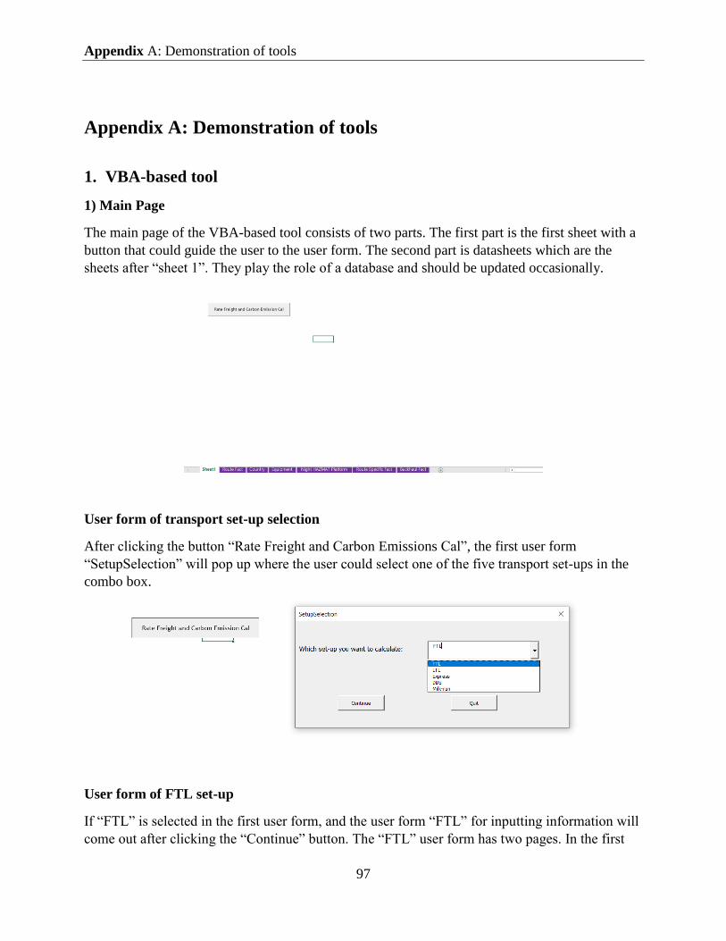
Appendix A: Demonstration of tools
97
Appendix A: Demonstration of tools
1. VBA-based tool
1) Main Page
The main page of the VBA-based tool consists of two parts. The first part is the first sheet with a
button that could guide the user to the user form. The second part is datasheets which are the
sheets after “sheet 1”. They play the role of a database and should be updated occasionally.
User form of transport set-up selection
After clicking the button “Rate Freight and Carbon Emissions Cal”, the first user form
“SetupSelection” will pop up where the user could select one of the five transport set-ups in the
combo box.
User form of FTL set-up
If “FTL” is selected in the first user form, and the user form “FTL” for inputting information will
come out after clicking the “Continue” button. The “FTL” user form has two pages. In the first

Appendix A: Demonstration of tools
98
page “Data1”, there are two areas, user input and fact data, while in the second page “Data2”,
there is only fact data area. The user needs to provide all the needed information by either
selecting from combo boxes or typing in the text boxes in the “User Input” area. After that, the
user needs to click the “Get Data” button at the bottom to retrieve critical fact data from
datasheets according to the information he/she has provided.
Two of the critical fact data, distance and fuel index, are presented on the first page because they
are even more important than the other critical fact data. The other critical fact data are presented
on the second page.
If the user has checked all the information and makes sure they are correct, he/she can get the
results by clicking the button “Cal!” at the bottom.
2. Spreadsheets-based tool
Input and Result Sheet

Appendix A: Demonstration of tools
99
Part of the result sheet for FTL file is shown in the following figures. The cells between columns
A to column AO are the input area where users type all the required information. The area
between columns AU to column BM presents the results obtained from other calculation sheets,
while the area between column AQ and AS presents the final result for FTL set-up. The
calculation sheet for other set-ups follows the same structure and will not be presented in the
thesis.
Calculation Sheets
Some of the calculation sheets are shown in the following figure. The sheet “(L) FTL Travel
Should Cost” is the calculation sheet for the FTL line-haul module, while the following sheets
will calculation the figure for different elements. Some elements are merged into one sheet to
save some space.
The calculation sheet for fuel cost, maintenance and repair cost, and consuming material cost is
used as an example, which is shown in the following two figures. Between column A and column
K is the required information transferred from input and result sheet. The area between column R
and column AC is the fact data retrieved from the datasheet, while the results for cost elements
are shown from column M to column P. The calculation sheets for other modules and elements
keep the same structure and will not be presented in the thesis.

Appendix A: Demonstration of tools
100

Appendix B: VBA Code
101
Appendix B: VBA Code
Due to the limit on pages, only screenshots of part of the codes will be shown.

Appendix B: VBA Code
102

Appendix B: VBA Code
103

Appendix C: Question list for the semi-structured interview
104
Appendix C: Question list for the semi-structured interview
Could you explain more about the set-up DDS and its two legs?
Could you explain more about the following three terms used in the Volvo transport set-
ups: “backhaul”, “backward trip of a round trip” and “drop trailer (WoW)”? Also, could
you explain more about how they are considered in each of the transport set-ups?
Does Volvo own any hub on its own which can conduct the cross-dock operation or all
the hub are externally outsourced? If there are hubs owned by Volvo, should the cost
generated by the internal hubs be considered in this calculation framework?
Could you give us more information regarding the route engine we are using and the data
it can provide? How do you trust with this route engine?
Could you explain more about the digital platform cost that the calculation framework
should consider?
Could you explain more about the “payment term” of Volvo?
How do you think that this new tool/ framework for estimating the road freight rate can
contribute to your business operations?
What other functions would you like to have within this calculation framework and the
applicable tools?
What other internal data sources (e.g. reports, slides, database) can you share with us for
this study?

Appendix C: Question list for the semi-structured interview
105
Can you introduce the current tool for estimating the road freight rate? How does this
current tool perform and how do you trust in this current tool?
What could be the reasons for the gap between the real bid and the estimated rate for a
lane? Any insight from the business relation or other non-technical reasons?
Anything else that you would like to mention or stress?