A brief introduction into microbial communityanalysis using R

Roey Angel

30/01/2015

What is R and why should you use it?

From Wikipedia: “R is a programming language and softwareenvironment for statistical computing and graphics. The R languageis widely used among statisticians and data miners for developingstatistical software and data analysis. Polls and surveys of dataminers are showing R’s popularity has increased substantiallyin recent years.”

What is R and why should you use it?

Should you programme at all

I Reproducibility (track you analysis)I Automation (prepare for the future, update your analysis)I Communication (between you and the computer and between

you and other people)

What is R and why should you use it?

What can you do with R?

R, RStudio, and CRAN

R, RStudio, and CRAN

Loading OTU data tables and sequence data into Rand examining it

The most reliable and trouble–free method is to store primary datain text files in a tab-delimited or CSV form. The basic commandsfor loading data tables are:

read.table()

and

read.csv() #orread.csv2() # for comma decimals

The following functions help us examine the dataset

I print()I head()I In Rstudio View()

ExamplesOTU.table <- read.table(file = "OTU_table.txt", head = T,

row.names = 1)head(OTU.table, 3)

## Plant1_1 Plant1_2 Plant2_1 Plant2_2 Plant2_3 Plant3_1 Plant3_2## Otu0001 2144 1341 847 844 769 629 538## Otu0002 124 66 196 182 186 21 20## Otu0003 1593 1525 16 15 22 634 635## Plant3_3 Soil_1 Soil_2 Soil_3 Soil_4 Soil_5 Soil_6 Plant4_1## Otu0001 554 2591 1740 1395 1544 1468 2004 378## Otu0002 14 0 0 0 1 0 0 376## Otu0003 513 0 50 3 1 0 0 88## Plant4_2 Plant4_3 Plant5_1 Plant5_2 Plant6_1 Plant6_2## Otu0001 349 289 980 303 42 726## Otu0002 217 174 927 694 5190 282## Otu0003 50 38 6 32 32 1239

Examples

View(OTU.table)

Summarising the datasummary(OTU.table)

## Plant1_1 Plant1_2 Plant2_1 Plant2_2## Min. : 0.00 Min. : 0.00 Min. : 0.00 Min. : 0.00## 1st Qu.: 0.00 1st Qu.: 0.00 1st Qu.: 0.00 1st Qu.: 0.00## Median : 0.00 Median : 0.00 Median : 0.00 Median : 0.00## Mean : 3.96 Mean : 3.96 Mean : 3.96 Mean : 3.96## 3rd Qu.: 0.00 3rd Qu.: 0.00 3rd Qu.: 1.00 3rd Qu.: 1.00## Max. :2144.00 Max. :1525.00 Max. :847.00 Max. :844.00## Plant2_3 Plant3_1 Plant3_2 Plant3_3## Min. : 0.00 Min. : 0.00 Min. : 0.00 Min. : 0.00## 1st Qu.: 0.00 1st Qu.: 0.00 1st Qu.: 0.00 1st Qu.: 0.00## Median : 0.00 Median : 0.00 Median : 0.00 Median : 0.00## Mean : 3.96 Mean : 3.96 Mean : 3.96 Mean : 3.96## 3rd Qu.: 1.00 3rd Qu.: 0.00 3rd Qu.: 0.00 3rd Qu.: 0.00## Max. :769.00 Max. :822.00 Max. :889.00 Max. :837.00## Soil_1 Soil_2 Soil_3 Soil_4## Min. : 0.00 Min. : 0.00 Min. : 0.00 Min. : 0.00## 1st Qu.: 0.00 1st Qu.: 0.00 1st Qu.: 0.00 1st Qu.: 0.00## Median : 0.00 Median : 0.00 Median : 0.00 Median : 0.00## Mean : 3.96 Mean : 3.96 Mean : 3.96 Mean : 3.96## 3rd Qu.: 0.00 3rd Qu.: 0.00 3rd Qu.: 0.00 3rd Qu.: 0.00## Max. :2591.00 Max. :1740.00 Max. :1395.00 Max. :2505.00## Soil_5 Soil_6 Plant4_1 Plant4_2## Min. : 0.00 Min. : 0.00 Min. : 0.00 Min. : 0.00## 1st Qu.: 0.00 1st Qu.: 0.00 1st Qu.: 0.00 1st Qu.: 0.00## Median : 0.00 Median : 0.00 Median : 0.00 Median : 0.00## Mean : 3.96 Mean : 3.96 Mean : 3.96 Mean : 3.96## 3rd Qu.: 0.00 3rd Qu.: 0.00 3rd Qu.: 0.00 3rd Qu.: 1.00## Max. :1468.00 Max. :2004.00 Max. :1125.00 Max. :893.00## Plant4_3 Plant5_1 Plant5_2 Plant6_1## Min. : 0.00 Min. : 0.00 Min. : 0.00 Min. : 0.00## 1st Qu.: 0.00 1st Qu.: 0.00 1st Qu.: 0.00 1st Qu.: 0.00## Median : 0.00 Median : 0.00 Median : 0.00 Median : 0.00## Mean : 3.96 Mean : 3.96 Mean : 3.96 Mean : 3.96## 3rd Qu.: 1.00 3rd Qu.: 0.00 3rd Qu.: 0.00 3rd Qu.: 0.00## Max. :572.00 Max. :980.00 Max. :1005.00 Max. :5190.00## Plant6_2## Min. : 0.00## 1st Qu.: 0.00## Median : 0.00## Mean : 3.96## 3rd Qu.: 0.00## Max. :1239.00

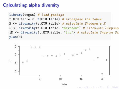
Calculating alpha diversity

library(vegan) # load packaget.OTU.table <- t(OTU.table) # transpose the tableH <- diversity(t.OTU.table) # calculate Shannon's HD <- diversity(t.OTU.table, "simpson") # calculate Simpson's DiD <- diversity(t.OTU.table, "inv") # calculate Inverse Simpsonplot(H)

5 10 15 20

2.5

3.5

4.5

5.5

Index

H

Calculating rarefaction curvesrarecurve(t.OTU.table, step = 20, col = "blue", cex = 0.6)

0 2000 4000 6000 8000 10000

020

040

060

080

0

Sample Size

Spe

cies

Plant1_1Plant1_2

Plant2_1Plant2_2Plant2_3

Plant3_1Plant3_2Plant3_3

Soil_1Soil_2Soil_3Soil_4Soil_5

Soil_6Plant4_1

Plant4_2Plant4_3

Plant5_1

Plant5_2

Plant6_1

Plant6_2

rarefy(t.OTU.table, min(rowSums(t.OTU.table)))

## Plant1_1 Plant1_2 Plant2_1 Plant2_2 Plant2_3 Plant3_1 Plant3_2 Plant3_3## 397 373 887 893 886 555 549 547## Soil_1 Soil_2 Soil_3 Soil_4 Soil_5 Soil_6 Plant4_1 Plant4_2## 630 618 626 592 547 614 598 713## Plant4_3 Plant5_1 Plant5_2 Plant6_1 Plant6_2## 737 307 397 167 397## attr(,"Subsample")## [1] 10122

Ploting rank abundancerad <- rad.lognormal(t.OTU.table )plot(rad, xlab = "Rank", ylab = "Abundance")

0 2000 4000 6000 8000 10000 12000

15

1050

100

500

5000

Rank

Abu

ndan

ce

Beta diversitybeta <- vegdist(t.OTU.table, binary=TRUE)pcoa.obj <- capscale(t.OTU.table ~ 1, distance = "bray")plot(pcoa.obj)text(scores(pcoa.obj)$sites[,1], scores(pcoa.obj)$sites[,2],

labels=rownames(t.OTU.table))

−2 −1 0 1

−1.

0−

0.5

0.0

0.5

1.0

MDS1

MD

S2

+

+

++

+

+

+

+

+

+

+

+

+

+

+

++

+

+

++

+++

++ ++ +

+++

++ +

+

+

++

+++

+++ +

++

+ ++++ ++++

+

+++++ ++

+

+

+ +

+

+ ++++++

+ ++++

+ ++++

+

++

++++ +++

+ ++++

+++

++ ++++ +++++

+++++++ +++ +++

++ +++++++

++++++

++ ++++++++++++

++++++++++++++

++++++++++++++++++++++++++++++++++++++++++++++++++++++++++++++++++++++++++++++++++++++++++++++++++++++++++++++++++++++++++++++++++++++++++++++++++++++++++++++++++++++++++++++++++++++++++++++++++++++++++++++++++++++++++++++++++++++++++++++++++++++++++++++++++++++++++++++++++++++++++++++++++++++++++++++++++++++++++++++++++++++++++++++++++++++++++++++++++++++++++++++++++++++++++++++++++++++++++++++++++++++++++++++++++++++++++++++++++++++++++++++++++++++++++++++++++++++++++++++++++++++++++++++++++++++++++++++++++++++++++++++++++++++++++++++++++++++++++++++++++++++++++++++++++++++++++++++++++++++++++++++++++++++++++++++++++++++++++++++++++++++++++++++++++++++++++++++++++++++++++++++++++++++++++++++++++++++++++++++++++++++++++++++++++++++++++++++++++++++++++++++++++++++++++++++++++++++++++++++++++++++++++++++++++++++++++++++++++++++++++++++++++++++++++++++++++++++++++++++++++++++++++++++++++++++++++++++++++++++++++++++++++++++++++++++++++++++++++++++++++++++++++++++++++++++++++++++++++++++++++++++++++++++++++++++++++++++++++++++++++++++++++++++++++++++++++++++++++++++++++++++++++++++++++++++++++++++++++++++++++++++++++++++++++++++++++++++++++++++++++++++++++++++++++++++++++++++++++++++++++++++++++++++++++++++++++++++++++++++++++++++++++++++++++++++++++++++++++++++++++++++++++++++++++++++++++++++++++++++++++++++++++++++++++++++++++++++++++++++++++++++++++++++++++++++++++++++++++++++++++++++++++++++++++++++++++++++++++++++++++++++++++++++++++++++++++++++++++++++++++++++++++++++++++++++++++++++++++++++++++++++++++++++++++++++++++++++++++++++++++++++++++++++++++++++++++++++++++++++++++++++++++++++++++++++++++++++++++++++++++++++++++++++++++++++++++++++++++++++++++++++++++++++++++++++++++++++++++++++++++++++++++++++++++++++++++++++++++++++++++++++++++++++++++++++++++++++++++++++++++++++++++++++++++++++++++++++++++++++++++++++++++++++++++++++++++++++++++++++++++++++++++++++++++++++++++++++++++++++++++++++++++++++++++++++++++++++++++++++++++++++++++++++++++++++++++++++++++++++++++++++++++++++++++++++++++++++++++++++++++++++++++++++++++++++++++++++++++++++++++++++++++++++++++++++++++++++++++++++++++++++++++++++++++++++++++++++++++++++++++++++++++++++++++++++++++++++++++++++++++++++++++++++++++++++++++++++++++++++++++++++++++++++++++++++++++++++++++++++++++++++++++++++++++++++++++++++++++++++++++++++++++++++++++++++++++++++++++++++++++++++++++++++++++++++++

Plant1_1 Plant1_2

Plant2_1Plant2_2Plant2_3

Plant3_1Plant3_2Plant3_3

Soil_1

Soil_2

Soil_3Soil_4Soil_5

Soil_6

Plant4_1Plant4_2Plant4_3

Plant5_1

Plant5_2

Plant6_1

Plant6_2

Easy and fency analysis using phyloseq

Easy and fency analysis using phyloseq

source("http://bioconductor.org/biocLite.R")biocLite("phyloseq")

library(phyloseq)taxonomy <- read.table(file = "OTU_table_taxonomy.txt",

head = T, row.names = 1)OTU <- otu_table(OTU.table[1:50, ], taxa_are_rows = TRUE)TAX <- tax_table(as.matrix(taxonomy[1:50, ]))(physeq <- phyloseq(OTU, TAX))

## phyloseq-class experiment-level object## otu_table() OTU Table: [ 50 taxa and 21 samples ]## tax_table() Taxonomy Table: [ 50 taxa by 6 taxonomic ranks ]

Bar graph of OTUsplot_bar(physeq, fill = "Order")

0

2000

4000

6000

8000

Plant1_1

Plant1_2

Plant2_1

Plant2_2

Plant2_3

Plant3_1

Plant3_2

Plant3_3

Plant4_1

Plant4_2

Plant4_3

Plant5_1

Plant5_2

Plant6_1

Plant6_2

Soil_1

Soil_2

Soil_3

Soil_4

Soil_5

Soil_6

Sample

Abu

ndan

ce

Order

Acidimicrobiales

Bacillales

Burkholderiales

Caulobacterales

Corynebacteriales

Cytophagales

Frankiales

Kineosporiales

Micrococcales

Myxococcales

Propionibacteriales

Pseudomonadales

Rhizobiales

Rhodobacterales

Sphingobacteriales

Sphingomonadales

Streptomycetales

Subgroup

Unclassified

Xanthomonadales

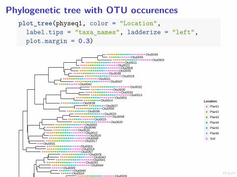
Phylogenetic tree with OTU occurencesplot_tree(physeq1, color = "Location",

label.tips = "taxa_names", ladderize = "left",plot.margin = 0.3)

Otu0001

Otu0002

Otu0003

Otu0004

Otu0005

Otu0006

Otu0007

Otu0008

Otu0009

Otu0010

Otu0011

Otu0012

Otu0013

Otu0014

Otu0015

Otu0016

Otu0017

Otu0018

Otu0019

Otu0020

Otu0021

Otu0022

Otu0023

Otu0024

Otu0025

Otu0026

Otu0027

Otu0028

Otu0029

Otu0030

Otu0031

Otu0032

Otu0033

Otu0034

Otu0035

Otu0036

Otu0037

Otu0038

Otu0039

Otu0040

Otu0041

Otu0042

Otu0043

Otu0044

Otu0045

Otu0046

Otu0047

Otu0048

Otu0049

Otu0050

Location

a

a

a

a

a

a

a

Plant1

Plant2

Plant3

Plant4

Plant5

Plant6

Soil

Plot heat mapsplot_heatmap(physeq1, taxa.label = "Class")

SphingobacteriiaAcidimicrobiiaActinobacteriaActinobacteria

UnclassifiedGammaproteobacteria

AlphaproteobacteriaDeltaproteobacteria

AcidimicrobiiaActinobacteria

AlphaproteobacteriaAlphaproteobacteriaBetaproteobacteria

AlphaproteobacteriaSphingobacteriia

AcidimicrobiiaAlphaproteobacteria

ActinobacteriaAlphaproteobacteria

ActinobacteriaCytophagia

AlphaproteobacteriaActinobacteria

SphingobacteriiaAlphaproteobacteria

UnclassifiedActinobacteria

BetaproteobacteriaBetaproteobacteria

SphingobacteriiaSphingobacteriia

AlphaproteobacteriaSphingobacteriia

GammaproteobacteriaSphingobacteriia

AlphaproteobacteriaSphingobacteriia

AlphaproteobacteriaAcidobacteria

AlphaproteobacteriaSphingobacteriia

AcidobacteriaAcidobacteria

BacilliAlphaproteobacteria

ActinobacteriaSphingobacteriia

GammaproteobacteriaAlphaproteobacteria

Bacilli

Soil_5

Soil_2

Plant1_1

Plant3_2

Plant3_1

Plant3_3

Plant1_2

Plant2_2

Plant2_3

Plant2_1

Plant5_1

Plant5_2

Plant6_2

Plant4_2

Plant4_3

Plant6_1

Plant4_1

Soil_1

Soil_3

Soil_6

Soil_4

Sample

Cla

ss

1

16

256

4096Abundance

Links

http://www.r-project.org/

http://www.rstudio.com/

http://cran.r-project.org/web/packages/vegan/index.html

https://joey711.github.io/phyloseq/