a branch and bound algorithm for the knapsack problem · pdf filemanagement science vol. 13,...

MANAGEMENT SCIENCE Vol. 13, No. 9, May, 1967

Printed in U.S.A.

A BRANCH AND BOUND ALGORITHM FOR THE KNAPSACK PROBLEM *t

PETER J. KOLESAR

Columbia University

A branch and bound algorithm for solution of the "knapsack problem," max E vzix where E wixi < W and xi = 0, 1, is presented which can obtain either optimal or approximate solutions. Some characteristics of the algorithm are discussed and computational experience is presented. Problems involving 50 items from which approximately 25 items were loaded were solved in an average of 0.07 minutes each by a coded version of this algorithm for the IBM 7094 computer.

1. Introduction

This paper presents a branch and bound algorithm for the solution of a special type of combinatorial problem. The problem which is sometimes called the knapsack problem arises in various cargo loading situations and consists of selecting from a finite collection of objects that subcollection which maximizes a linear function of the objects selected while obeying a single linear inequality constraint.

This problem may be formulated and solved in a variety of ways. The method proposed here is of interest in that it provides initially a solution which is approximately optimal and also an upper bound on the value of the optimal solution. Thus, computation may be terminated at any point where it is felt that further improvements in the solution are not worth the additional computational effort. The nature of the algorithm is such that the approximation tends to be good for problems involving a large number of items where each item makes a small contribution to the objective function and to the restriction. Further, it appears that the efficiency of the algorithm increases as the size of the problem increases. Nonetheless, as with other branch and bound [8] algorithms, the memory and time requirements are quite large for problems involving many items.

As will be shown in Part 2 of this paper, the problem may be formulated as an integer linear programming problem and may be solved using either the all integer cutting plane method of Gomory [5] or the more specialized algorithm of Balas [7] for linear programs with 0, 1 variables. Still another approach to the problem is offered by dynamic programming, and Bellman and Dreyfus [2] have treated slightly different versions of the problem in this way. Fulkerson has formulated the problem as a network flow problem. The solution is obtained by finding the longest chain of an acyclic network. Although this is a quite straight-

* Received March 1966 and revised November 1966. t Research supported in part by the Office of Naval Research under contract Nonr 266

(55), and the National Science Foundation under grant GP 2202. Reproduction in whole or in part is permitted for any purpose of the United States Government.

723

724 PETER J. KOLESAR

forward task, a disadvantage of this method is that a very large network is generated if the contributions of the items to the restriction vary widely. Gilmore and Gomory [5] have used a "branch and exclude" method based upon ideas of Benders. The Gilmore-Gomory method is similar to the method presented here which exploits the "branch and bound" concepts applied by Little, et al. [13], to the travelling salesman problem. The method of implicit enumeration or "branching and bounding" is also employed for solution of the more general 0, 1 integer programming problem by many writers including [1], [6], [13].

2. The Problem

Suppose that we wish to select from among a finite collection of indivisible objects a subcollection which maximizes a linear function subject to a linear inequality constraint. This problem may be viewed as a simple version of situations which occur in some cargo loading operations. However, there are a variety of other applications: Hansmann [9] in a capital investment context, Kolesar [11] in a network reliability problem, Gilmore and Gomory [5] in a cutting stock problem, and Cord [3] in a capital budgeting problem have all explicitly used the knapsack problem as a model.

Consider a collection of N indivisible objects, labelled by the integers i = 1, 2, ... N. With each object is associated a positive real number wt, the "weight" of the object, and real number vi, the "value" of the object. It is desired to form a loading of the objects by selecting from among the N objects a subcollection which has a maximum total value but which does not exceed a total weight of say W units. The problem may be stated mathematically as follows: Find xi, i 1, 2, .., N such that

(1) Maximize Nxtv

subject to

(2) t x ii W

(3) Xi = 8 or 1, i 1, 2,... ,N.

The problem, thus formulated, is an integer linear programming problem and may be solved as such. Further, since there are only a finite number of indivisible objects which are to be arranged into two groups (those loaded and those not loaded), there are only a finite (although possibly a very large) number of possible solutions, and an algorithm which proceeds by successive partitions of the class of all possible solutions will work, at least in theory. In the discussion that follows, we assume that a feasible solution exists; that is that (2) and (3) are satisfied for some {xi}. An implicit assumption that vi > 0, wi _ 0, W > 0 implies that xi = 0 i 1, * * * , N is trivally feasible. One can easily verify at the outset if a nontrivial feasible solution exists by the following:

A nontrivial feasible solution exists if and only if

A BRANCH AND BOUND ALGORITHM FOR THE KNAPSACK PROBLEM 725

3. The Algorithm

We call the algorithm which will be proposed here a branch and bound algorithm in the sense of Little, et al. [13]. In the following paragraphs we introduce some terminology and notation, discuss generally the concepts on which the branch and bound algorithm is based, and then present the details of the specific branching and bounding procedure proposed.

General

We adopt the following terminology. A collection of xi satisfying xi _ 1, i = 1, 2, * , N and (2) will be called a solution or a loading. Notice that this permits violation of the assumption that each item is indivisible. A collection of xi satisfying (2) and (3), that is, obeying the indivisibility assumption, will be called a feasible solution.

A branch and bound algorithm proceeds by repeatedly partitioning the class of all feasible solutions into smaller and smaller subclasses in such a way that ultimately an optimal solution is obtained. The partitioning, or branching as it is called, is carried out so that at each partitioning the subclasses of solutions are mutually exclusive and all inclusive, that is, each feasible solution belongs to exactly one subclass. For each of the subclasses of solutions one computes an upper bound to the maximum value of the objective function attained by solutions belonging to the subclass. On the basis of these upper bounds, a further stage of branching is carried out, new upper bounds are computed, and so on, repeatedly, until ultimately a feasible solution is obtained which has a value of the objective function greater than the upper bounds of all the subclasses and also higher than the values of the objective function for all previously obtained solutions. The algorithm is constructive in nature. It repeats the branching process, successively generating smaller and smaller subclasses some of which ultimately will contain only one feasible solution, one of which will be optimal.

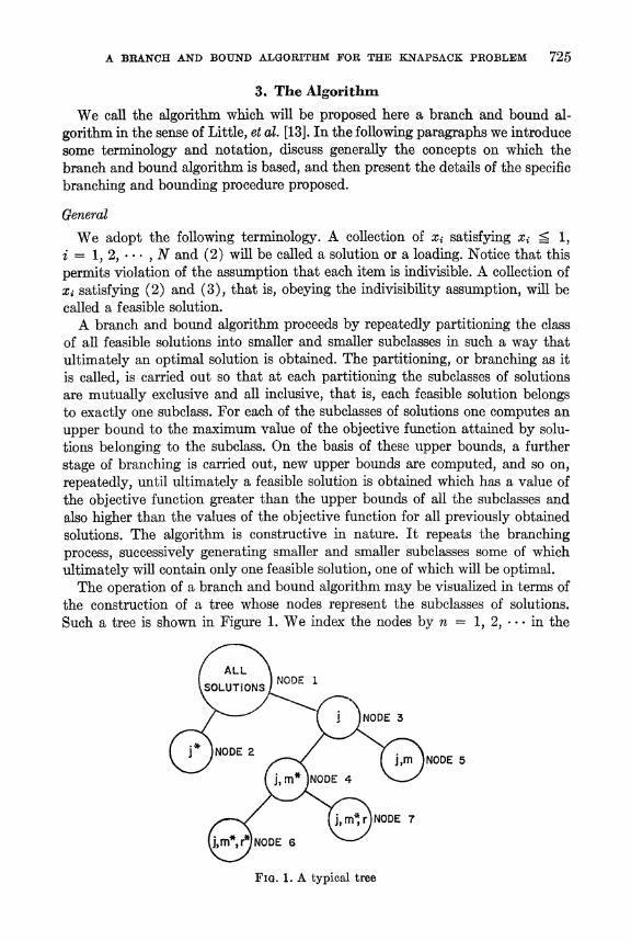
The operation of a branch and bound algorithm may be visualized in terms of the construction of a tree whose nodes represent the subclasses of solutions. Such a tree is shown in Figure 1. We index the nodes by n 1, 2, *. in the

ALL

SOLUTIONS NODE L FIG. 1. AtypicalNODE 3

X NODE 2 ND 5

( im NODE 4

/ ( j~, m*r) NODE 7

ANODE 6

FIG. 1. A typical tree


order in which they are generated by the algorithm. We denote by B(n) the upper bound associated with node n. A node that has not been branched from is a terminal node. Branching takes place at the terminal node which has the highest value of B(n) and is accomplished by creating two new descendent nodes.

We describe a node, that is a subclass of feasible solutions, by listing the items which are explicitly included in the solutions (loadings) contained in the subclass, and the items which are explicitly excluded from the solutions which are contained in the subclass. Thus at a given node n, we speak of three categories of items:

Included Items

The set of items which are explicitly included in the solutions contained in node n will be denoted by In~ . In Figure 1 we indicate the members of I," at each node by listing their indices.

Excluded Items

The set of items which are explicitly excluded from the solutions contained in node n will. be denoted by E,,. In Figure 1 we indicate the members of E,, at each node by listing their indices with star superscripts.

Unassigned Items

The items which belong to neither I,, or to E. have not yet been specifically assigned. When the set of unassigned items at any node 'is empty, the node con- tains only one solution and further branching from that node is impossible.

Branching at a node takes place in the following way: One of the previously unassigned items is selected; in one descendent node it becomes included and in the other it becomes excluded. Upon performing the branching, the algorithm checks the feasibility of the solutions contained in the two new nodes. If the subclass of solutions contained in a given node is infeasible, further branching from that node is eliminated; if the subclass of solutions is feasible, the upper bound is computed and the process continues. The details of the branching and bounding processes are given below.

In the same tree shown in Figure 1, node 1 represents the class of all feasible solutions. Node 2 represents all feasible solutions which do not include item j, while node 3 represents all feasible solutions which do include item j. Node 7 represents all feasible solutions containing j and r but not m. The sets I, , E,, for the nodes shown in Figure 1 are:

I2 (O E2=(j)

14(j) E4 (M)

15 =(j,rm) E5 =0


16 = (i) E6 = (m, r)

17 = (j, r) E7 = (m)

Rules for Branching and Bounding

The computation of upper bounds is based upon two observations. The first is that the relaxation of the restriction of indivisibility on one or more of the items results in a new optimization problem whose optimum value of the objective function cannot be smaller than the optimum value of the objective function for the original problem. The second observation is that for a loading problem in which all of the items are perfectly divisible, that is:

(4) maximize i=y YiVi

subject to

(5) y iwyi < M

(6) 0 < Y i < 1,

an optimum solution is obtained by arranging the items in decreasing order of magnitude of the ratio vi/ws, and then, starting with the first item on this list, sequentially loading as much as possible of each item until the weight limit M is reached.

We now apply these two facts to the computation of upper bounds. Suppose that we are at a node n, with the sets I,, and En as defined above being, respec- tively, the sets of items included and excluded from the solutions. All other items are unassigned. Prior to computing the upper bound at node n, we test the feasibility of the class of solutions contained in the node by verifying if

(7) ein Wi <_ W.

No further computations will be made at nodes which do not satisfy (7). In order to compute the upper bound at node n, we assert that it is sufficient to solve the following problem:

(1) maximize E '=1 Xivi subject to

(2) X < TW

(8) X = 1, iEIn

(9) Xi = 0, iEEn

(10) 0 < Xi < 1 iE(InUEn)

The solution of this system is an upper bound at node n by application of the first observation since in (10) we have relaxed restriction (3) for the unassigned items at node n. The second observation gives a direct solution to this system since by a simple transformation it can be put in the form of (4), (5), (6). The solution is given by:


(a) Order all items in (IrzUEn)c by decreasing vl/wi and starting with the first item in this list load as much as possible of each item in sequence until the total weight of the items so loaded exactly equals W - E win , .

(b) The upper bound at node n, B(n), is equal to the total value loaded in (a) above plus EZa, v .

In order to perform the branching operation, two decisions must be made. First, one must select the terminal node at which to make the next branch, and second one must select the item which will be added to the list of included and excluded items in the two resulting descendent nodes. We call this the "pivot" item. The selection of the node at which to make the next branch is clearly dictated by the branch and bound method to be the terminal node with the highest value of B(n). On the other hand, selection of the pivot element is arbi- trary. Clearly, one would like to make this selection in a manner that would enable the algorithm to reach an optimum solution as soon as possible. The solution to (4), (5), (6) suggests an heuristically good choice. Assuming that the original items have been arranged according to decreasing order of magnitude of vl/wi , we select as the pivot element the unassigned variable with largest vl/w . In the case of a tie, select that item which appears first in the sequence.

4. Outline of the Algorithm

The following instructions outline the operations and decisions involved in the algorithm:

Stage 1 (Preliminary)

(a) Test the nontrivial feasibility of the problem by verifying at least one indexi = 1,2,... ,N,

Wi < W

If the problem is nontrivially feasible, proceed to (b), if not, stop. (b) If Z~=i wi < W, then all items may be loaded and the problem is trivial.

If not, proceed to (c) (c) Order the items by decreasing magnitude of vl/w2. In all that follows

we assume that the items have been so ordered. Proceed to (d) (d) For node 1 set B(1) = 0, IA = sn, = s. Proceed to Stage 2.

Stage 2 (Selection of Node for next Branching)

(a) Find the terminal node with the largest value of B(n). This is the node at which the next branching will take place.

(b) Test if at the current node k, (IkUEk)c = sp. If so, an optimal solution is given by the indices contained in Ik . If not, select the new pivot item i* by,

-= i such that

vi/w, is a max for ie(IkUEk)6

Proceed to stage 3(a).


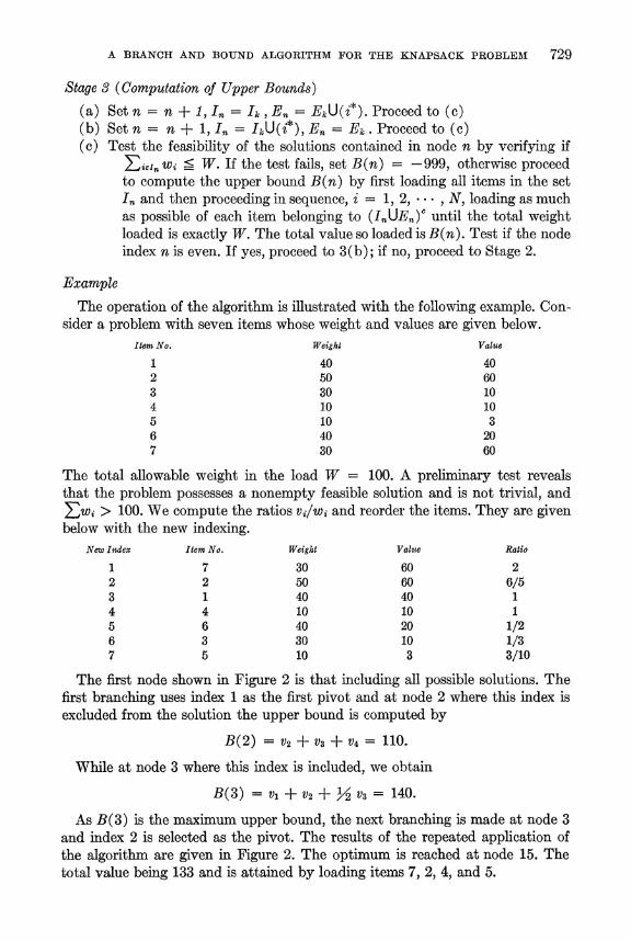
Stage 3 (Computation of Upper Bounds)

(a) Set n = n + 1, In = Ik, E. = EkU(i*). Proceed to (c) (b) Set n = n + 1 In = IkU(i*), En = Ek . Proceed to (c) (c) Test the feasibility of the solutions contained in node n by verifying if

Eieln wi < W. If the test fails, set B(n) = -999, otherwise proceed to compute the upper bound B(n) by first loading all items in the set In and then proceeding in sequence, i = 1, 2, * * *, N, loading as much as possible of each item belonging to (In UEn)Y until the total weight loaded is exactly W. The total value so loaded is B(n). Test if the node index n is even. If yes, proceed to 3(b); if no, proceed to Stage 2.

Example

The operation of the algorithm is illustrated with the following example. Con- sider a problem with seven items whose weight and values are given below.

Item No. Weight Value

1 40 40 2 50 60 3 30 10 4 10 10 5 10 3 6 40 20 7 30 60

The total allowable weight in the load W = 100. A preliminary test reveals that the problem possesses a nonempty feasible solution and is not trivial, and Ewi > 100. We compute the ratios v/lwi and reorder the items. They are given below with the new indexing.

New 1hdex Itemn No. Weight Value Ratio

1 7 30 60 2 2 2 50 60 6/5 3 1 40 40 1 4 4 10 10 1 5 6 40 20 1/2 6 3 30 10 1/3 7 5 10 3 3/10

The first node shown in Figure 2 is that including all possible solutions. The first branching uses index 1 as the first pivot and at node 2 where this index is excluded from the solution the upper bound is computed by

B(2) = V2 + V3 + V4 = 110.

While at node 3 where this index is included, we obtain

B(3) = VI + V2 + Y2 V3 = 140.

As B(3) is the maximum upper bound, the next branching is made at node 3 and index 2 is selected as the pivot. The results of the repeated application of the algorithm are given in Figure 2. The optimum is reached at node 15. The total value being 133 and is attained by loading items 7, 2, 4, and 5.


NODE 14 2 2,3 ( ( 1 l) O-

NODE 2 i _2 < \NODE 3 B(2)X10 1silo1 B(3) 140

NODE j4 NODE

B(14):130459120 5,6 7 5 4

z < NODE 7T ,.

NODE 6 for (7 ea 999

B(8)6= 135(ND

NODE ) = 1332 NODE 9

NQDE NOD 12 /NODE I 3,

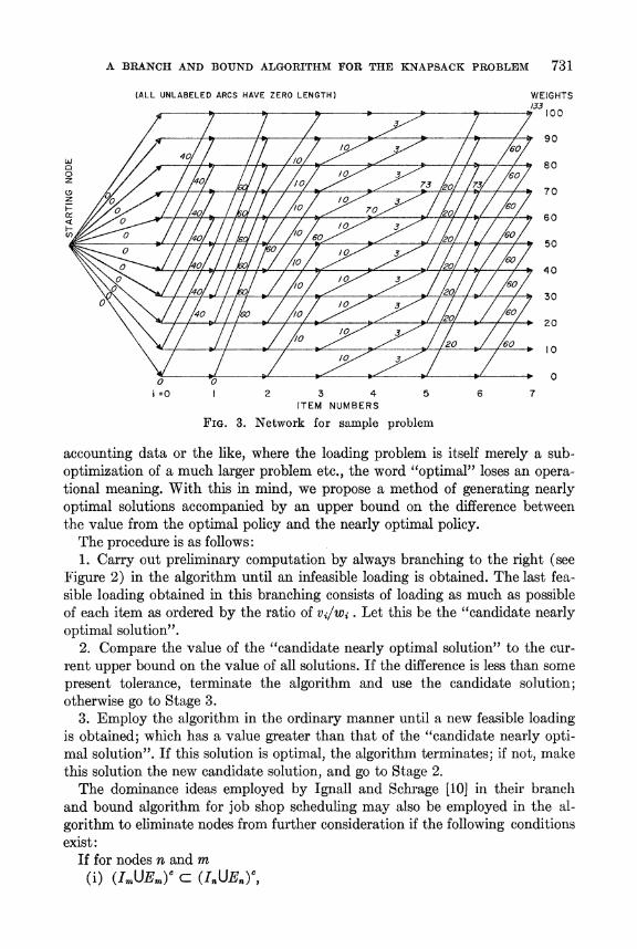
For purposes of comparison, we present the network flow solution to this example. The problem is that of finding the largest chain in the following acyclic network. The nodes of the network are denoted by the couple (i, w) where i denotes the index of the i2 item i = 0, 1, *--, N and w takes on all integers w =0, 1, *- W. We assume that the item weights are normalized to integers. Each node (i, w) has two arcs leading into it. One arc leads from node (i -1, w) and has length zero; the second arc leads from node (i -1, w - w) and has length vi. We add to the network a starting node which is Joined to all nodes (0, w) with arcs of length zero. Thus a chain from the starting node to node (i, w) corresponds to a subset of the first items whose total weight is w and the length of the chain is the total value of the subset. The network for this example is given in Figure 3.

5. Modifications of the Algorithm

Iln certain loading problems there may be no practical advantage to getting al optimal loading if a nearly optimal loading is available. In fact, in some situations where the "weights" w f and/of the "values" vs are estimated from


(ALL UNLABELED ARCS HAVE ZERO LENGTH) WEIGHTS

(00

90

0 ~~~~~~~~~~~~~~~~~~~~80 0~~~~~~~~~~~~~~~~~~~7

0 7~~~~~~~~~~~~~~~~~~0

30

2 0

0~~~~~~~~~~~~~~~~~~~~~~I 0 4 0~~~~~~/

0 0 ~~~~~~~~~~~~~~~~~~~~~~~~30

i=0 I 2 3 4 5 6 7 ITEM NUMBERS

FIG. 3. Network for sample problem

accounting data or the like, where the loading problem is itself merely a sub- optimization of a much larger problem etc., the word "optimal" loses an opera- tional meaning. With this in mind, we propose a method of generating nearly optimal solutions accompanied by an upper bound on the difference between the value from the optimal policy and the nearly optimal policy.

The procedure is as follows: 1. Carry out preliminary computation by always branching to the right (see

Figure 2) in the algorithm until an infeasible loading is obtained. The last feasible loading obtained in this branching consists of loading as much as possible of each item as ordered by the ratio of vi/ws. Let this be the "candidate nearly optimal solution".

2. Compare the value of the "candidate nearly optimal solution" to the current upper bound on the value of all solutions. If the difference is less than some present tolerance, terminate the algorithm and use the candidate solution; otherwise go to Stage 3.

3. Employ the algorithm in the ordinary manner until a new feasible loading is obtained; which has a value greater than that of the "candidate nearly optimal solution". If this solution is optimal, the algorithm terminates; if not, make this solution the new candidate solution, and go to Stage 2.

The dominance ideas employed by Ignall and Schrage [10] in their branch and bound algorithm for job shop scheduling may also be employed in the algorithm to eliminate nodes from further consideration if the following conditions exist:

If for nodes n and m (i) (ImUEm)C C (InuEn)c,


(ii) Ei'in Vi -Eia.m Vi , (iii) EiCIn Wi < ie'r. WiX

then node n dominates node m since it has at least as high a value of the objective function, has at least as much unused capacity, and has at least the same unassigned items.

6. Extension of the Algorithm Linus Schrage has suggested that the algorithm can be modified slightly to

handle the following more general problem: maximize

EZ==1 Vi(yi) subject to

ZX== Wi(yi) < W

yi = 0, 1, 2, *--

where Wi(yi) is a monotonically increasing function of yi and vi(yi) is an arbi- trary function of yi. The problem may be formulated as a kind of knapsack problem by representing

yi = Ej xij where xij = 0, 1. However, the additional constraint xij > xij+l may be neces- sary to assure that the jth of a given item type is loaded if the j + lt is loaded. In cases in which the objective function is concave and the constraints define a convex set, the constraint may not need to be explicitly employed. In cases in which the constraint must be explicitly employed, one can define for node n a set Cn of unassigned but unassignable items and then compute upper bounds by solving ordinary linear programming problems of the form: maximize

i= Xtii

subject to

zjX=1x 1 i < W

where

xi = 1 for icIn

i= 0 for icEn

0 ? XL ? 1 for i(InUEn)cUCn .

The next pivot item must be selected from the set IcflnEncflncz. In [11] Kolesar treats a problem of optimal design of redundancy in networks which are subject to two types of failure by formulating the problem as a knapsack problem having order relationships between the variables.


7. Computational Experience

The version of the algorithm presented in Section 4 has been coded in Fortran IV for the IBM 7094 computer. Branch and bound algorithms involve a signifi- cant amount of list processing for which Fortran is not designed. Consequently, our code is relatively unsophisticated and becomes inefficient as the number of nodes generated becomes large. It is possible to construct a code which would solve larger problems more efficiently.

Approximately 500 sample problems have been generated and solved on the IBM 7094 computer. The number of items ranged from 3 to 100. Item weights and values were generated randomly as approximately independent observations on a normally distributed random variable with expected value of 5.00 and standard deviation of 0.91. The algorithm was run until either an optimal solution was obtained or until the node list reached 3000.

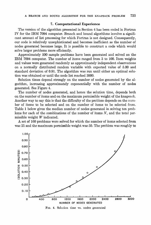
Solution times depend strongly on the number of nodes generated by the algorithm, increasing approximately exponentially with the number of nodes generated. See Figure 4.

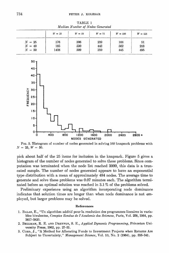
The number of nodes generated, and hence the solution time, depends both on the number of items and on the maximum permissible weight of the knapsack. Another way to say this is that the difficulty of the problem depends on the number of items to be selected and on the number of items to be selected from. Table 1 below gives the median number of nodes generated in solving ten problems for each of the combinations of the number of items N, and the total permissible weight W indicated.

A set of 160 problems were solved for which the number of items selected from was 25 and the maximum permissible weight was 50. The problem was roughly to

1.00

0.90 /

0.80 _

W 0.70 -

Z 0.60 -

z 0.50 - 0

D 0.40-

0 0.30 -

0.20 -

0.10 _

0 400 800 1200 1600 2000 2400 2800 3200 NUMBER OF NODES GENERATED

FIG. 4. Solution time vs. nodes generated


TABLE 1 Median Number of Nodes Generated

W= 25 W= 50 W= 75 W= 100 W= 125

N= 25 176 306 239 168 51 N = 40 185 530 443 562 213 N = 50 1408 509 359 445 495

50

45

40-

35-

0>- 30- z

=>25- 0

2 20-.

15-

10-

5-

0A 0 400 800 1200 I600 2000 2400 2800 +

NODES GENERATED

FIG. 5. Histogram of number of nodes generated in solving 160 knapsack problems with N = 25, W = 50.

pick about half of the 25 items for inclusion in the knapsack. Figure 5 gives a histogram of the number of nodes generated to solve these problems. Since computation was terminated when the node list reached 3000, this data is a trun- cated sample. The number of nodes generated appears to have an exponential type distribution with a mean of approximately 484 nodes. The average time to generate and solve these problems was 0.07 minutes each. The algorithm terminated before an optimal solution was reached in 3.1 % of the problems solved.

Preliminary experience using an algorithm incorporating node dominance indicates that solution times are longer than when node dominance is not employed, but larger problems may be solved.

References

1. BALAS, E., "Un algorithm additif pour la resolution des programmes lineaires in variables bivalentes, Comptes Rendus de l'Academic des Sciences, Paris, Vol. 258, 1964, pp. 3817-3820.

2. BELLMAN, R. E. AND DREYFUS, S. E., Applied Dynamic Programming, Princeton Uni- versity Press, 1962, pp. 27-31.

3. CORD, J., "A Method for Allocating Funds to Investment Projects when Returns Are Subject to Uncertainty," Management Science, Vol. 10, No. 2 (1964), pp. 335-341.


4. FULKERSON, D. R., Flow Networks and Combinatorial Operations Research, Memoran- dum RM-3378, Oct. 1962, The RAND Corp.

5. GILMORE, P. C. AND GOMORY, R. E., "A Linear Programming Approach to the Cutting Stock Problem-Part II," Operations Research, Vol. 11 (1963), pp. 863-888.

6. GLOVER, F., "A Multiphase Dual Algorithm for the Zero-One Integer Programming Problem," Operations Research, Vol. 13 (1965), pp. 879-919.

7. AND ZOINTS, STANLEY, "A Note on the Additive Algorithm of Balas," Operations Research, Vol. 13 (1965), pp. 546-549.

8. GOMORY, R. E., "An All Integer Programming Algorithm," in J. R. Muth and G. L. Thompson (Eds.), Industrial Scheduling, Prentice-Hall, 1963.

9. HANSMANN, F., "Operations Research in the National Planning of Underdeveloped Countries," Operations Research, Vol. 9 (1961), pp. 203-248.

10. IGNALL, E. AND SCHRAGE, L., "Application of the Branch and Bound Techniques to Some Flow Shop Scheduling Problems," Operations Research, Vol. 13, No. 3 (1965), pp. 400-412.

11. KOLESAR, P., "Assignment of Optimal Redundancy in Systems Subject to Failure," Columbia University, Operations Research Group, Technical Report, 1966.

12. LAWLER, E. L. AND WOOD, D. E., "Branch and Bound Methods: A Survey," Operations Research, July-August, 1966.

13. LITTLE, J. D. C., MURTY, K. G., SWEENEY, D. W. AND KAREL, C., "An Algorithm for the Travelling Salesman Problem," Operations Research, 1963, pp. 972-989.

a branch and bound algorithm for the knapsack problem · pdf filemanagement science vol. 13,...

Documents