at SciVerse ScienceDirect

Environmental Modelling & Software 43 (2013) 144e159

Contents lists available

Environmental Modelling & Software

journal homepage: www.elsevier .com/locate/envsoft

A box model of the seasonal exchange and mixing in Regions ofRestricted Exchange: Application to two contrasting Scottish inlets

P.A. Gillibrand a,*, M.E. Inall a, E. Portilla b, P. Tett a

a Scottish Association for Marine Science, Scottish Marine Institute, Oban, Argyll PA37 1QA, UKb School of Life Sciences, Edinburgh Napier University, 10 Colinton Road, Edinburgh EH10 5DT, UK

a r t i c l e i n f o

Article history:Received 1 February 2012Received in revised form20 November 2012Accepted 3 February 2013Available online 13 March 2013

Keywords:FjordFlushing timeExchange rateExchange processesStratified inlet

* Corresponding author. Present address: CSIROResearch, GPO Box 1538, Hobart TAS 7001, Australia. T3 62325000.

E-mail address: philip.gillibrand@csiro.au (P.A. Gil

1364-8152/$ e see front matter � 2013 Elsevier Ltd.http://dx.doi.org/10.1016/j.envsoft.2013.02.008

a b s t r a c t

We present a time-dependent box model of exchange and mixing processes in Regions of RestrictedExchange (RREs). The model is applied to two contrasting Scottish inlets, but can potentially be applied toa wide range of stratified inshore water bodies. The model represents the vertical structure of the inletusing up to three horizontally uniform layers, representing surface, intermediate and deep basin waterrespectively, and calculates the daily volume, thickness, salinity and temperature of each layer over anannual cycle. The model is forced by observed time series of daily-mean wind stress, river discharge,surface heat flux, and depth-profiles of the external coastal temperature and salinity. Advective anddiffusive fluxes between the layers, and between the inlet and adjacent coastal ocean, are calculated fromparameterisations of known physical processes in inshore stratified waters, utilising published analyticalsolutions and empirically-based formulae. The goal is for the model to be generally applicable to RREs tosupport improved resource management. As such, the number of free parameters within the model hasbeen kept to a minimum.

The model predictions of layer temperature and salinity are quantitatively compared to observationsfrom year-long sampling programmes in two contrasting Scottish inlets, Loch Creran and Loch Etive. Themodel showed good agreement with the observed data, reproducing the broad scale seasonal cycle andother shorter-term fluctuations. RMS errors for temperature were less than 1 �C, and for salinity typicallyof the order 1. The model results suggest that Loch Creran behaved as a well-mixed box, with weakstratification maintained by strong vertical diffusion, and volume exchange between the inlet and coastalwaters dominated by tidal forcing. In contrast, Loch Etive exhibited classical fjordic three-layer hy-drography and dynamics, with strong stratification, weak vertical diffusion and a density-driven circu-lation comparable in strength to tidal exchange. The effects of a deep water renewal event on waterproperties were successfully reproduced by the model. The potential for wider application of the modelto resource management issues and to other types of RRE is discussed.

� 2013 Elsevier Ltd. All rights reserved.

1. Introduction

Regions of Restricted Exchange (RREs) are elongated stretches ofcoastal water penetrating inland at mid-high latitudes in bothnorthern and southern hemispheres (Tett et al., 2003). Examples ofRREs are the inlets of North America, the fjords of Scandinavia andChile, the rias of Spain, the voes and sea-lochs of Scotland, and theloughs of Ireland. RREs are typically bounded on three sides by land,with water exchange occurring only through the fourth, oftennarrow, boundary. Around the world, RREs have been subject to

Marine and Atmosphericel.: þ61 3 62325169; fax: þ61

librand).

All rights reserved.

increasing pressure from coastal development and coastal industry.In particular, the growth of finfish aquaculture in Europe, NorthAmerica, Scandinavia and Chile over the past four decades has beenconcentrated in RREs, and has raised considerable concerns overpotential impacts on the surrounding environment (Black, 2001).The concerns include benthic and water quality degradation due tocarbon and inorganic nutrient emissions, increased risk of eutro-phication in coastal waters, and the potentially toxic effects onnative flora and fauna of chemicals used by the aquaculture in-dustry. The potential risk to water quality in RREs is mitigated bythe strength of mixing and exchange, both internally within theRRE and externally between the RRE and the adjacent coastalocean. However, the external exchange in RREs is, by definition,restricted, which, while providing the sheltered waters favourablefor aquaculture infrastructure, may exacerbate water quality

Fig. 1. Schematic diagram of the three-layer conceptual model and the volume fluxesand layer parameters calculated. The layer parameters of thickness (Hj), volume (Vj),cross-sectional area (Xj), temperature (Ti) and salinity (Sj) are indicated, as are theadvective fluxes (QT, QG), entrainment fluxes (QH, QEij) and the vertical diffusive fluxes(QKij). The symbols are explained in the text. Also shown are the forcing data of riverdischarge (QF), wind speed (W), heat flux (QSHF) and external temperature and salinityprofiles (TO, SO). The deep water renewal switch, d, takes the value 0 or 1.

P.A. Gillibrand et al. / Environmental Modelling & Software 43 (2013) 144e159 145

problems. Much interest is focussed, therefore, by coastal managerson understanding and quantifying the mechanisms of water ex-change in these environments.

The processes that dominate exchange between RREs and theadjacent coastal ocean are the tides, a density-driven circulationcaused by both freshwater discharges into the RRE and fluctuationsin the coastal density profile (e.g. Arneborg, 2004), and deep waterrenewal in fjordic estuaries (Farmer and Freeland, 1983). Within anRRE, entrainment and mixing processes, caused by wind stirring,velocity shear and internal wave activity (e.g. Stigebrandt, 1976,1977; Farmer and Freeland, 1983; Simpson and Rippeth, 1993),redistribute water properties between surface and deep waterlayers. The net effect of these processes is to produce a water col-umn structure in RREs that can be effectively represented by two orthree horizontally- and vertically-uniform layers, separated byprimary and secondary pycnoclines. The upper two layers are inopen connectionwith the coastal ocean, whereas the third, bottom,layer may be isolated from the open ocean by the presence of a sill.This simplified water structure facilitates the use of relativelysimple models to quantify the dynamics of exchange in RREs. Thegoal of this paper is to develop a simple box-type model of RREexchange and mixing processes that can be widely applied tovarying types of RRE to inform resource management and toquantify the dominant mechanisms of exchange in differentsystems.

Simple box-type models can provide useful insights into thedynamics of coastal channels and inlets. Pawlowicz et al. (2007)used a mixing-box approach to determine residence times in theStrait of Georgia. The interannual variability of volume fluxes andwater properties between the Strait of Georgia and Juan de FucaStrait was investigated with a box model by Li et al. (1999) andBabson et al. (2006) studied the interannual variability of residencetimes of Puget Sound basins. Simpson and Rippeth (1993) used aone-dimensional (1D) model to quantify the contributions to themixing regime in the Clyde Sea, a Scottish inlet, by tides, convec-tion, wind stirring and internal waves. They found that the lattertwo processes dominated the seasonal mixing cycle. Finally,Stigebrandt (1985) developed a 1-Dmodel of the mixed layer depthfor the Baltic Sea, which particularly focussed on the balance be-tween surface layer mixing and buoyancy inputs. The physicalprocesses of horizontal and vertical exchange in Scandinavianfjords have been extensively investigated by Stigebrandt et al. overthe past three decades (e.g. Stigebrandt, 1980, 1981, 1985, 1999),culminating in the development of the FjordEnv model(Stigebrandt, 2001), a water quality model for inshore waters. Forwell-mixed and partially-mixed estuaries, box models using ex-change rates derived from observed salinity distributions (e.g.Officer, 1980) have been widely used, but such models are notappropriate for the present application due to the relative scarcityof hydrographic observations upon which the models fundamen-tally depend.

In this paper we present a model, ACExR, of physical exchangeprocesses in RREs with applications to two contrasting Scottishinlets. Although we focus here on Scottish inlets, we believe themodel is generally suited and easily adaptable to other RREs. Thephysical dynamics of Scottish inlets are not dissimilar to Scandi-navian fjords, and the mathematical framework of the FjordEnvmodel has provided a proven basis on which to build and developthe ACExR model. The ACExR model also utilises researchdescribing physical exchange and mixing processes in Scottish(Simpson and Rippeth, 1993; Rippeth and Simpson, 1996; Inall andRippeth, 2002; Inall et al., 2005) and Scandinavian (Liungman,2000; Arneborg, 2004) inlets. We present simulations of the sea-sonal cycle of water temperature, salinity and exchange in twocontrasting Scottish inlets: Loch Creran and Loch Etive. The

performance of the model is evaluated against available data, andthemodel is then used to describe the dynamical balance of the twosystems.

2. Description of the model

A schematic illustration of the model design is presented inFig. 1. RREs such as inlets and fjords can be considered to consist ofthree horizontally-uniform layers, representing a surface brackishlayer, an intermediate tidally-exchanged layer, and a bottom layerisolated from the adjacent coastal ocean by the presence of a sill.Other RREs, such as rias and voes, do not necessarily contain sillsand the isolated bottom water is not present; in these cases, thebottom layer can be excluded from the model and the water bodytreated as a two-layer system. The layers interact through exchangeof mass, volume and heat via a number of physical processes,indicated by the fluxes Q in Fig. 1. Daily variability in the calculatedtransports, together with surface forcing (Fig. 1), controls the evo-lution of the thickness, temperature and salinity of each layer overthe annual cycle.

Note that tidal exchange operates through the intermediatelayer. On each rising tide, seawater from outside the inlet entrancefloods into the inlet, sinking beneath the less dense surface waterinto the intermediate layer below. The outflowing surface layer isconsidered to be “arrested” by the incoming tidal current and istherefore stationary during flood tides (often leading to thedevelopment of “V-shaped” fronts above inlet sills e.g. Booth,1987).Therefore, in ACExR, tidal exchange is modelled as an exchangebetween the intermediate layer and the external coastal ocean(Fig. 1).

2.1. Model formulation

The framework for the model lies in the conservation of massand salt, coupled with parameterisations of the dynamical terms.Notation is given in Table 1. Conservation of volume, Vj, in layersj ¼ 1, 2, 3 is expressed as:

P.A. Gillibrand et al. / Environmental Modelling & Software 43 (2013) 144e159146

dV1

dt¼ QH þ QE12

dV2

dt¼ �QH � QE12 þ QE23

dV3

dt¼ �QE23

(1)

where QH is the vertical volume flux (m3 s�1) between layers 1 and2 due to wind stirring, and QEij is the vertical flux due to entrain-ment across the density interfaces between layers i and j due totidal velocity shear. Both the wind-stirring and entrainment terms(QH, QEij) can be positive (upward) or negative (downward).

Transport of a passive tracer Cj (for example temperature T, orsalinity S) in layer j (j ¼ 1, 2, 3) is given by:

dðVCÞ1dt

¼ QGðC2 � C1Þ þQFðCF � C1Þ þQHCi þQE12Ci þQK12ðC2 � C1Þ þV1G

dðVCÞ2dt

¼ �1� d

�QGðCO � C2Þ þ dQGðC3 � C2Þ þ

�1� d

�QTðCO � C2Þ �QHCi �QK12ðC2 � C1Þ þQK23ðC3 � C2Þ þQE23Ci �QE12Ci

dðVCÞ3dt

¼ dðQG þQTÞðCO � C3Þ �QK23ðC3 � C2Þ �QE23Ci

(2)

where QKij is the vertical flux (m3 s�1) due to turbulent mixing(eddy diffusion) between layers i and j, QT is the volume flux due totidal exchange, QF is the freshwater flux and G is the flux of Cthrough the surface boundary. For salinity, G ¼ 0 (evaporation andprecipitation are neglected), whereas for temperature, G ¼ QSHF/(Cp$r1$H1), where QSHF is the surface heat flux and Cp is the specificheat capacity of seawater. The tracer flux terms for QH and QEijflows, whichmay be positive or negative, use the upstreamvalue Ci,i ¼ 1, 2, 3. All the other volume flux (Q) terms are always positive.The switch d, which invokes the onset of deep water renewal, isdescribed below.

The term CO represents the external value of C (outside thewater body) and CF is the freshwater value. Presently, we set SF ¼ 0and (due to a general lack of riverine temperature data) TF ¼ T1 (i.e.the influence of freshwater temperature on surface layer temper-ature is neglected).

The surface heat flux, QSHF, is calculated from incident short-wave solar radiation, upward long-wave radiation, and sensibleand latent heat fluxes through the surface (Gill, 1982). Incidentradiation data were obtained from atmospheric observations madeat a nearby weather station (see Section 3). Long-wave radiationwas calculated from those observations according to Gill (1982, p.34). Sensible and latent heat fluxes were also calculated from theobservations using bulk parameterizations described by Fairallet al. (1996).

Water density in layer j, rj, is calculated from temperature andsalinity through a linear equation of state (Knauss, 1996):

rj ¼ rref�1� a

�Tj � 10

�þ b�Sj � 35

��(3)

where rref is a reference density, a is the thermal expansion coef-ficient (a ¼ 1.5 � 10�4 K�1) and b is the saline contraction coeffi-cient (b ¼ 7.8 � 10�4).

Equations (1)e(3) describe the temporal evolution of layervolume (and thickness), temperature, salinity and density, plus anyadditional simulated tracers. The volume flux terms are calculated

following published parameterisations from a range of sources asdescribed below.

2.1.1. Gravitational circulationThe strength of the density-driven estuarine circulation is here

related to the horizontal density gradient between the surfacewater inside and outside the estuary. This approach was adoptedpreviously by Simpson and Rippeth (1993) and Li et al. (1999). Thevolume transport is given by:

QG ¼ CGðr0 � r1Þ=rref (4)

where r0 is the external density and CG is a free constant (m3 s�1),which is tuned to provide a best fit to observations.

2.1.2. Tidal exchangeThe volume flux due to tidal exchange is given by

QT ¼ 2 3a0A0

TP(5)

where a0 is the tidal amplitude (m), A0 is the horizontal surface areaof the water body (m2), and TP is the dominant (e.g. M2) tidal period(s). The efficiency of tidal exchange (0 � 3� 1) is derived from theestuary exchange method of Wells and van Heijst (2003) i.e.

3¼ 1� ð4YS=pUSTPÞ1=2 YS=USTP � 0:13

3¼ 1 YS=USTP < 0:13(6)

where YS is the width of the entrance sill (m) and US the currentspeed over the entrance sill (m s�1), which for the current casestudies is known (Edwards and Sharples, 1986) but could bederived from QT and the known cross-sectional area of the entrancesill or channel. Wells and van Heijst (2003) derived (6) to accountfor the increased efficiency of estuary exchange when the entranceto the estuary is constricted and produces a jet-like flow on theflood tide. A jet-like flood tide injects external water into the es-tuary basin beyond the range from which water is drawn forejection on the subsequent ebb tide, thus increasing the efficiencyof the exchange process. If no entrance sill exists in the modelledsystem, 3defaults to unity.

2.1.3. Tidal entrainmentEntrainment is the process bywhich ambient fluid is transferred

across a density interface by, and incorporated into, a flowing layerof turbulent fluid. Entrainment is common in environmental flows(Turner, 1986). Here, we consider entrainment from the surface anddeep layers into the tidally energetic intermediate layer. As notedearlier, the outflowing surface layer is considered to be “arrested”by the incoming tidal current and is therefore stationary duringflood tides. The lower, deep water layer is quiescent. The turbulentintermediate layer therefore entrains fluid from above and below

Table 1List of symbols.

Symbol Description Units

t Time sVi Volume of layer i (i ¼ 1, 2, 3) m3

Hi Thickness of layer i mSi Salinity of layer i e

Ti Temperature of layer i �Cri Density of layer i kg m3

QH Vertical volume flux between layers 1 and 2, dueto wind-driven entrainment

m3 s�1

QEij Volume flux due to tidal and density drivenentrainment between layers i and j

m3 s�1

QKij Volume flux due to vertical mixing (eddy diffusion)between layers i and j

m3 s�1

QT Volume flux due to tidal exchange m3 s�1

QG Volume flux due to the gravitational estuarinecirculation

m3 s�1

QF Volume flux of freshwater discharged into the loch m3 s�1

QSHF Net heat flux through the water surface W m�2

KZij Vertical eddy diffusivity between layers i and j m2 s�1

Aij Horizontal interfacial area between layers i and j m2

A0 Horizontal surface area of the loch basin m2

Xi Vertical cross-sectional area of layer i m2

YS Width of the entrance sill mUS Current speed over the entrance sill m s�1

W Wind speed m s�1

TP Dominant (e.g. M2) tidal period sa0 Amplitude of the surface barotropic tide mg Acceleration due to gravity m s�2

a Thermal expansion coefficient,a ¼ (1/r0)vr/vT ¼ 1.46 � 10�4

K�1

b Saline contraction coefficient,b ¼ (1/r0)vr/vS ¼ 7.60 � 10�4

e

d Switch indicating whether deep water renewal isoccurring (d ¼ 1) or not (d ¼ 0)

e

CP The specific heat capacity of seawater, CP ¼ 4200 J kg�1 K�1

B Surface buoyancy flux m2 s�3

CD Drag coefficient ¼ 0.0025 e

CDS Surface drag coefficient ¼ 0.0015 e

CG Constant in the gravitational estuarine circulationtransport equation

m3 s�1

CE Constant in the wind-stirred entrainment equation e

3 Efficiency of tidal exchange e

l, m, g Constants in the vertical diffusivity equations(Equations (15) and (16))

e

ra Density of air, ra ¼ 1.3 kg m�3

rref The density of seawater at 10 �C and salinity of 35,rref ¼ 1027

kg m�3

r0 External water density kg m�3

u* Friction velocity m s�1

we Entrainment velocity due to wind stirring and buoyancyinputs

m s�1

wij Entrainment velocity between layer i and j due to tidalcurrent shear

m s�1

P.A. Gillibrand et al. / Environmental Modelling & Software 43 (2013) 144e159 147

during flood tides, depending on the strength of the velocity shearand the stratification across the interfaces. During ebb tides,stratification increases due to tidal straining, and entrainment isassumed to be inhibited. We have tested several entrainment al-gorithms developed from laboratory studies by Turner (1986) andStrang and Fernando (2001), but the results presented here usedthe algorithm presented by Princevac et al. (2005) for natural flows.The entrainment velocity normal to the horizontal interface, wij, iscalculated as:

wij

�x; t

�¼ 0:05U2Ri

�0:75B (7)

where RiB ¼ DBH2/DU2 is a bulk Richardson number, a balancebetween the buoyancy jump DB ¼ (g/rref)Dr and velocity shear DUacross the interface. Because, in the current conception of themodel, the surface layer is assumed to be stationary during flood

tide, DU is identical to U2. The intermediate layer velocity iscalculated as:

U2 ¼ ðQG þ QTsin utÞ=X2 (8)

where u¼ 2p/TP, and X2 is the cross-sectional area of layer 2. WhenU2 < 0 (i.e. during ebb tide),wij is set to zero. From the entrainmentvelocity, the vertical entrainment flux, QEij, is calculated as:

QEij ¼ Aijwij (9)

2.1.4. Wind-driven entrainmentThe balance between wind stirring and a positive vertical

buoyancy flux drives an entrainment velocity, we, at the base of thesurface layer. Following Stigebrandt (1985), who described a modelof the seasonal mixed layer for a large fjordic system, the Baltic,based on the KatoePhillips entrainment velocity, we specify:

we ¼ 2CEu3*

gDrrref

H1

� B

gDrrref

; B > 0 (10)

where B is the buoyancy input (see below), CE is a free constant, andu* is the friction velocity (m s�1) given by:

u2* ¼ rar1:CDS$W

2 (11)

where W is the wind speed (m s�1), CDS a surface drag coefficientand ra the density of air. The buoyancy flux through the sea surfaceis given by:

B ¼ g�

a

r1CPQSHF þ bS1

QF

A0

(12)

When the buoyancy input exceeds wind stirring, makingwe< 0,thewater column re-stratifies, and the pycnocline relaxes towards adepth equivalent to the MonineObukhov length (Stigebrandt,1985) i.e.

H1 ¼ 2CEu3*=B (13)

Thus when we < 0, the downward velocity is maintained untilthe surface layer thickness reaches H1, at which point we is set tozero until effectivewind stirring resumes orH1 reduces further. Thevertical volume flux between layers 1 and 2 due to wind stirring,QH, is therefore given by:

QH ¼ A12$we (14)

where A12 is the horizontal interfacial area (m2) between layers 1and 2.

2.1.5. Vertical eddy diffusionA further vertical flux of scalar water properties between layers

(there is no net volume flux) occurs as a result of vertical turbulentmixing driven by vertical velocity shear. We assume that KZS takesthe general form

KZS ¼ KZ0ð1þ gRiBÞl (15)

where KZ0 is the diffusivity of non-stratified flow, RiB is the bulkRichardson Number as defined above, and g and l are constants.Values of KZS must be calculated for mixing across both interfaces.The form of (15) is analogous to well-known open ocean parame-terisations of vertical mixing (e.g. Munk and Anderson, 1948;Lozovatsky et al., 2006), which used a gradient Richardson

P.A. Gillibrand et al. / Environmental Modelling & Software 43 (2013) 144e159148

Number rather than the bulk RichardsonNumber used here. Babsonet al. (2006) derived a vertical mixing formulation with the sameformas (15),with l¼�1, for their layeredboxmodel of Puget Sound,and we use (15) as an initial approximation of the vertical diffusiveflux. Following Babson et al. (2006), the value of KZ0 is given by

KZ0 ¼ mCDU2H2 (16)

where CD is a typical drag coefficient with a value of 0.0025 (Babsonet al., 2006) and m is a free parameter for calibration.

The shear-induced vertical mixing between model layers 2 and3 given by (15) is supplemented by an additional term, KZb, repre-senting the mixing caused by breaking internal waves in fjord ba-sins (Stigebrandt and Aure, 1989; Stigebrandt, 2001; Inall andRippeth, 2002; Cottier et al., 2004; Inall et al., 2004). The calcula-tion of KZb for silled fjords has been described in detail byStigebrandt (1999) and we do not repeat the mathematics here. Inbrief, each sill in the RRE system is assumed to generate a linearinternal tide in the stratified water column, and the energy flux iscalculated for each one. A small fraction of the total energy flux,generated at all the sills in the system, is expended on verticalmixing; we follow Stigebrandt (1999, 2001) and assume a mixingefficiency (flux Richardson Number) of 5% for ‘wave basins’ and 1%for ‘jet-type’ basins. The vertical diffusive fluxes are therefore givenby

KZ12 ¼ KZS

KZ23 ¼ KZS þ KZb(17)

and the volume transport due to vertical eddy diffusion is:

QKij ¼ AijKZij=Hij (18)

Here the overbar indicates the mean of Hi and Hj.

2.1.6. Deep water renewalA particular feature of themodel is the capability to simulate the

effects of deep water overturn or renewal events, which occurwhen the external water density, r0, becomes greater than thebottom density, r3. Renewal is a critical process for the exchange ofdeep water in fjord basins. In ‘normal’ conditions, when r0 < r3,gravitational and tidal exchange are confined to the surface andintermediate layers above sill depth. The intruding waters intolayer 2 entrain water from layer 3, so that the thicknesses of layer 2increases and that of layer 3 decreases. The water properties oflayer 3 are modified only by this entrainment process and verticaleddy diffusion. When water denser than the basin water (i.e.r0 > r3) crosses the entrance sill, a deep-water renewal event istriggered (Gade and Edwards, 1980), and the intruding water flowsdown the slope inside the sill, typically as a gravity current,entering the bottom layer. The ambient basin water is lifted up inthe water column, from where it can be exchanged and exit theinlet basin. The renewing water fills up the deep basin until thedensity of the external water is no longer sufficiently dense toreplenish the basin.

In the model, the deep-water renewal process is accomplishedby setting the switch d in Equation (2) to unity when r0 > r3.Otherwise, when r0 < r3, d ¼ 0. When d ¼ 1, the density-driven andtidal exchanges are directed into layer 3 rather than layer 2, asreflected in the transport of external water properties (Equation(2)). Density currents are well known to entrain fluid from theambient environment (Turner, 1986); in the model, the entrain-ment term QE23 is made negative, to reflect the downwardentrainment from layer 2 into layer 3 during renewal events. Thesimulated renewal event continues until either r0 < r3, or the

vertical location of the interface between layers 2 and 3 is elevatedto sill depth, at which point d is reset to zero. The approachdescribed here clearly does not simulate the dynamics of deepwater renewal events; our intention is only to attempt to reproducethe effects of the renewal process onwater properties in this simplemodel.

2.2. Boundary conditions

The model is forced by daily or hourly wind stress at the surface,total daily freshwater discharge into the surface layer and, if surfaceheat flux is to be included in the simulation, daily values of local sealevel pressure, air temperature, dew-point or wet-bulb tempera-ture, relative humidity, cloud cover and solar irradiation arerequired. These are used to derive the net daily heat flux, QSHF, intothe surface layer of the modelled inlet.

For the open boundary condition, daily profiles of coastal oceantemperature and salinity, external to the modelled basin, arerequired. In U.K. coastal waters, data of this frequency are few andfar between. More common, though by no means widespread, aremonitoring stations which may be sampled weekly or fortnightly.The model has beenwritten to accept available low-frequency dataand interpolate these data linearly into daily resolution. Linearinterpolation represents the simplest method of interpolatingsparse data, and makes the fewest assumptions about the nature ofthe data. However, it could be argued that data with a predictableseasonal cycle, for example coastal temperature, could be inter-polated using a sinusoidal curve, and that option may be added tothe model in future.

2.3. Solution procedure and implementation

Equations (1)e(18) form a closed set of equations that can besolved iteratively from an initial set of conditions to calculate Vi, Si,Ti and ri. From the hypsography of the model domain, the layerthickness, Hi, can be derived from Vi. The parameters CG in (4), CE in(10), l, g in (15) and m in (16) are free parameters that can be used tocalibrate the model. They control the strength of, respectively, theestuarine circulation, wind-driven entrainment and verticalmixing.

Initial values of Hi, Si and Ti must be specified. From these, Vi andri are derived. The model uses an Euler forward scheme in time,with a time step of Dt presently set to 0.1 days. A 5-day spin-upperiod is typically invoked. The tidal entrainment terms arecalculated using a sub-time-stepping procedure to ensure stability.Values of the forcing data QT and QF are derived, or supplied, at adaily resolution. Values of QG, QH, QW, QEij, QKij are calculated everytime step. At each time step, the values of all the transport variablesare first calculated using the most recent values of the layer prop-erties. The layer volume and thickness, Vi and Hi, are then updated,followed by Ti, Si and ri. At the end of each simulated day, values ofthe layer properties and the daily-mean values of the transportterms are stored.

The model was coded in the Mathworks MATLAB� scriptinglanguage, and can be operated under Windows, Mac and linuxoperating systems. The model is written in modular form,allowing easy modification and development of individual com-ponents of the code. A one-year simulation takes about twominutes.

2.4. Evaluation of model performance

The ability of the model to reproduce the observations is testedquantitatively. First, themodel results are linearly regressed againstthe corresponding observed data and the coefficient of the

P.A. Gillibrand et al. / Environmental Modelling & Software 43 (2013) 144e159 149

regression, r2, is determined. Second, we calculate the root meansquare error between model and data, given by

ERMS ¼241N

0@XN

j¼1

�pj � oj

�21A351=2

(19)

where pj and oj are predicted and observed values respectively andN is the number of data points in the calculation. Model skill isestimated using an index of agreement, d2 (Willmott et al., 1985):

d2 ¼ 1�24XN

j¼1

�pj � oj

�235,24XN

j¼1

�pj � oþ oj � o

�235

(20)

where o is the arithmetic mean of the observed data. A perfectagreement between model and data would give d2 ¼ 1, withdecreasing values indicating declining performance.

2.5. Ensemble simulations

The model was run repeatedly, with values of CG, CE, l, g and m

chosen at random from prescribed ranges. For both modelled sys-tems, Loch Creran and Loch Etive, an ensemble of 5000 memberswas performed. The ensemble approach allowed us to identify theparameter set that best reproduced the observations, and toinvestigate the sensitivity of the model to the empirical constants.The index of agreement, d2, was calculated for temperature andsalinity in each layer for every ensemble member. From these sixvalues, an overall (average) skill for the ensemble member wasderived, enabling the best parameter set to be identified for eachinlet system modelled.

In addition to the ensemble approach, some simulations testingthe sensitivity of the model to the boundary conditions were

Fig. 2. Locations of observation stations C2eC6 in Loch Creran and RE1eRE8 in Loch Etive onLoch Etive lies between RE5 and RE6. The locations of the monitoring station LY1, which pstaffnage and Tiree are also marked.

performed. The density of these fjordic RREs is dominated bysalinity, which in turn is controlled by the open ocean boundarycondition and the riverine freshwater input. Given the scarcity, inparticular, of adequate coastal ocean data, we tested the response ofthe model to the open boundary condition by repeating the twosimulations with constant coastal temperature and salinity values.The values chosen were the mean values of the data for 1978 and2000 for the Creran and Etive simulations respectively. Thus a ver-tical gradient was maintained, but remained constant throughoutthe simulations. Similarly, the simulations were repeated withconstant freshwater inputs (again, mean values for 1978 and 2000were used), and finally, simulations were performed with both theopen boundary conditions and river flows constant.

3. Observations

The model has been applied to two contrasting inlets inwestern Scotland: Loch Crean and Loch Etive (Fig. 2). These siteswere chosen largely on the basis of data availability, which arerequired both to force the model and evaluate the results. LochCreran has been the subject of a sporadic observation programmeover four decades. We have chosen to model 1978, when one ofthe most comprehensive annual datasets was collected (Tyler,1983). Loch Creran is a small inlet, about 13 km long, with amaximum water depth of 42 m (Table 2). It contains three sills, ofwhich the entrance sill is the shallowest with a maximum depthof 7 m. Loch Creran has a relatively low freshwater input, with arelatively small watershed (164 km2) compared to its surface area(15.1 km2).

Freshwater discharge data into Loch Creran during 1978 werederived from gauged flow on the River Creran by Tyler (1983),accounting for the increased catchment area of the loch relativeto the river and local variations in climatological rainfall be-tween individual river catchments. Wind speed data were ob-tained from the Tiree meteorological station and atmospheric

the west coast of Scotland. The sill in Loch Creran lies seaward of C2; the Bonawe sill inrovided boundary data for the Creran simulations, and the weather stations at Dun-

Table 2Keymodel parameter values for the two study sites, Loch Creran and Loch Etive. Thevalues for the five free parameters (CE, CG, m, g, l) are from the simulations whichproduced the highest model skill assessment scores.

Parameter Loch Creran Loch Etive

L (km) 13.1 30.0A0 (km2) 15.1 16.1Hmax (m) 42 140Catchment (km2) 164 1350YS (m) 325 188US (m s�1) 0.82 0.66T (s) 44,712 44,712a0 (m) 1.65 0.9CE 0.86 0.59CG 4.0 � 104 5.0 � 104

m 2.90 1.94g 0.10 0.28l �2 �2

P.A. Gillibrand et al. / Environmental Modelling & Software 43 (2013) 144e159150

variables required for heat flux calculations were recorded atDunstaffnage. The coastal temperature and salinity profiles camefrom station LY1 in the Firth of Lorn, which was sampled once ortwice each month during 1978. The forcing data for Loch Creranfrom 1978 are shown in Fig. 3.

Model results were compared with field observations of watertemperature and salinity. Full depth profiles of temperature andsalinity at six fixed stations in Loch Creran (C1eC6, Fig. 2) wererecorded at regular intervals throughout 1978 (Table 3). Here, weused data from 4 m (the shallowest depth consistently available),10 m and 40 m depths, as representative of layers 1, 2 and 3respectively, to compare against the model results. We did not usedepth-averaged data since the thickness of each model layer wasnot known a priori. The arithmetic-mean of the data from allstations inside the loch (C2eC6) was calculated to give a basin-average value. Depth-integrated data could not be used because

Fig. 3. Daily boundary data from 1978 used to force the physical exchange model for a simulnet surface heat flux (QSHF, W m�2), external coastal temperature (TE, �C), salinity (SE) and

of the variable thickness of the model-predicted layers. Boundaryforcing data consisted of profiles of temperature and salinity ob-tained at station LY1 (Fig. 2) during the same surveys of stationsC2eC6.

Loch Etive is one of the larger Scottish inlets, with a length of30 km and a maximum depth of 140 m (Table 2). It has six sills,the entrance sill being the shallowest with a maximum depth of7 m. This sill, known locally as “The Falls of Lora”, has a strongchoking effect on the tide, reducing the external spring tidalrange from 3.6 m to 1.8 m inside the inlet. The deepest basin lieslandward of the sixth sill, with the sill itself located between RE5and RE6 (Fig. 2). The sill depth is 13 m. Loch Etive has a largewatershed of 1350 km2 compared to its surface area of 29 km2,with much of the freshwater discharging via the River Awe closeto station RE5; the water in the inlet is more brackish (deepwater salinity values are typically 27) than is usual in Scottishinlets.

From July 1999eMarch 2001, the REES experiment in Loch Etivewas conducted by the Scottish Association for Marine Science(SAMS unpublished data). We used data from 2000 when thefield programme continued throughout the calendar year, withregular (approximately monthly) sampling trips to Loch Etive(Table 3). During each trip, conductivityetemperatureedepth(CTD) profiles were made and water samples collected at fixedstation locations, named RE1eRE8 (Fig. 2). To force the model,gauged flow data from the River Awe during 2000 were adjustedto account for the whole Etive catchment. Wind speed data camefrom the Tiree meteorological station, atmospheric variables fromDunstaffnage, and the coastal temperature and salinity profilescame from REES CTD station RE6 (Fig. 2). The model was used tosimulate only the upper basin of the loch, upstream of the sill atBonawe. [Experiments to run the model for the whole of LochEtive using data from RE8 as boundary forcing were not successful.The model failed to run due to the extreme flow speeds and

ation of Loch Creran: riverine freshwater discharge (QF, m3 s�1), wind speed (W, m s�1),density (st, kg m�3) at 4 depths (1, 10, 20, 30 m).

Table 3Sampling dates in each of the two simulated years for the two lochs, Creran andEtive. The date, and the Julian day, of each observation are given. See text forobservation depths. The means of all available station data at each depth and sampledate were used to generate a basin-average for comparison with the modelpredictions.

Loch Creran, 1978 Loch Etive, 2000

Date J. day Date J. day

16 January 1978 16 12 January 2000 1230 January 1978 30 22 February 2000 5313 February 1978 44 29 March 2000 9027 February 1978 58 16 April 2000 1086 March 1978 65 6 June 2000 1593 April 1978 93 11 July 2000 19317 April 1978 107 11 August 2000 22415 May 1978 135 14 September 2000 25829 May 1978 149 15 October 2000 28912 June 1978 163 6 November 2000 3123 July 1978 184 13 December 2000 34917 July 1978 19831 July 1978 21214 August 1978 22628 August 1978 24011 September 1978 2549 October 1978 28225 October 1978 2986 November 1978 31018 December 1978 352

P.A. Gillibrand et al. / Environmental Modelling & Software 43 (2013) 144e159 151

turbulence that occur over the sill at the Falls of Lora; theconfiguration and application of the model to the whole of LochEtive remains a challenging problem]. The forcing data are shownin Fig. 4.

Data from depths of 3 m (the shallowest data depth consistentlyavailable), 15 m and 110 m at RE1eRE5 were averaged to providerepresentative values for each layer. As with Loch Creran, we didnot use depth-averaged data since the thickness of each modellayer was not known a priori.

Fig. 4. Daily boundary data from 2000 used to force the physical exchange model for a simunet surface heat flux (QSHF, W m�2), coastal temperature (TE, �C), salinity (SE) and density (

4. Results

4.1. Model calibration, evaluation and sensitivity

Observed water temperatures from Loch Creran in 1978 weredominated by the mid-latitude seasonal cycle (Fig. 5). Surfacetemperatures ranged from 5.5 �C in February (Days 32e60) toalmost 14 �C in summer. In the intermediate and deep layers, thetemperature range was slightly less, with marginally warmerwinter temperatures and cooler summer ones. However, observa-tions at each depth co-varied strongly, and thermal stratification inthe water column was evidently weak throughout the year. Littlehigh-frequency variability in temperature was apparent from theobservations, either due to inadequate sampling frequency or anabsence of such variability. The observations indicate a smoothlyvarying temperature cycle over the year. The salinity of the watercolumnwas less affected by the seasonal cycle andwas drivenmoreby discharge events. The salinity data reveal three major fresheningevents during 1978, in January (Days 16e30), April (Day 93) andOctobereNovember (Days 282e310). These events clearly occurredin response to periods of increased river discharge (Fig. 3). Eachevent was clearly evident throughout the water column, and thesalinity difference between surface and deep water was generallyless than 2, again suggesting relatively weak stratification of thewater column throughout the year.

The ensemble spread for the Loch Creran simulation was quiteconfined (Fig. 5), indicating that for this system the model wasrelatively insensitive to the free parameter values. The predictedtemperature in particular, for all three model layers in Loch Creran,was very consistent between ensembles. Water temperature vari-ability was dominated by the external coastal temperature and theseasonal heating cycle. The predicted salinity time series for LochCreran showed greater ensemble spread, but were still quite tightlyconfined around the best simulation. As we shall see below, LochCreran acts as a rather well-mixed box, and the internal dynamics

lation of Loch Etive: riverine freshwater discharge (QF, m3 s�1), wind speed (W, m s�1),st, kg m�3) at 4 depths (1, 10, 20, 30 m) at location RE6.

Fig. 5. Predicted temperature (a, c, e) and salinity (b, d, f) time series for three waterlayers in Loch Creran for 1978. All 5000 individual ensemble members are shown asthin grey lines. The solid black line indicates the overall ‘best fit’ simulation. Observeddata, from Tyler (1983), are indicated by the open circles.

P.A. Gillibrand et al. / Environmental Modelling & Software 43 (2013) 144e159152

have rather little effect on its water properties. The system couldconceivably be modelled accurately by a much simpler, single-boxmodel, and the sensitivity of the model predictions to chosenparameter values is limited.

The model skill assessment suggests that the model predictedtemperature better than salinity, with higher d2 values and RMSerrors that were a smaller fraction of the observed standard devi-ation (Table 4). In each layer, temperature was predicted with anRMS error of less than 1 �C. In late spring and summer, predictedtemperatures in the surface and intermediate layers were slightlywarmer than observed, with RMS errors of 0.63 �C and 0.73 �Crespectively. But the model predictions compared well with datathrough autumn andwinter, and overall the seasonal cyclewaswell

Table 4Standard deviation (SD) of the data, and the regression correlation coefficient (r2),root-mean-square error (ERMS) and model skill (d2) for the model predictions oftemperature, salinity and density in the three model layers for each simulation.

Temperature Salinity

SD r2 ERMS d2 SD r2 ERMS d2

Loch Creran 1978Layer 1 2.88 0.96 0.63 0.988 1.25 0.74 0.64 0.919Layer 2 2.75 0.96 0.73 0.984 1.05 0.83 0.54 0.932Layer 3 2.57 0.99 0.24 0.998 0.80 0.74 0.51 0.844

Loch Etive 2000Layer 1 3.50 0.88 1.54 0.941 7.97 0.95 1.81 0.983Layer 2 2.27 0.91 0.91 0.964 5.04 0.97 1.15 0.984Layer 3 1.03 0.76 0.52 0.927 0.48 0.97 0.41 0.888

reproduced. The deep water temperature was very accuratelypredicted throughout the year (RMS error ¼ 0.24 �C).

Themodel largely reproduced the threemajor freshening eventsobserved during 1978. In the surface and intermediate layers, theminimum predicted salinity was less than the minimum observedsalinity, but the predicted minima occurred slightly earlier theobserved ones and it is possible that the discrepancy is due tounder-sampling; the model salinity at the time of the observedminima matched the observed values closely. In the deep layer, theagreement between model and data during these events was lessgood, with the predicted salinities being too high. Overall, salinityin Loch Creran for 1978 was reproduced satisfactorily, with RMSerrors less than 1, and skill score for the surface and intermediatelayers exceeding 0.9 (Table 4). The model successfully reproducedthe key features of the observed system: a strong seasonal cycle intemperature, major freshening events in the salinity records, andrelatively weak thermal and haline stratification.

In Loch Etive during 2000, observations again revealed a strongseasonal cycle in both temperature and salinity in the surface andintermediate layers, both having lower values during winter andrising over spring and summer (Fig. 6). Over the seasonal cycle, thewater temperature and salinity in the surface layer varied overranges of 10 �C and 20 respectively; the seasonal variability of bothparameters was slightly reduced in the intermediate layer. In thebottom layer, no seasonality was evident, with changes in waterproperties dominated by a deep water renewal event during days

Fig. 6. Predicted temperature (a, c, e) and salinity (b, d, f) time series for three waterlayers in Loch Etive for 2000. All 5000 individual ensemble members are shown as thingrey lines. The solid black line indicates the overall ‘best fit’ simulation. Observed dataare indicated by the open circles.

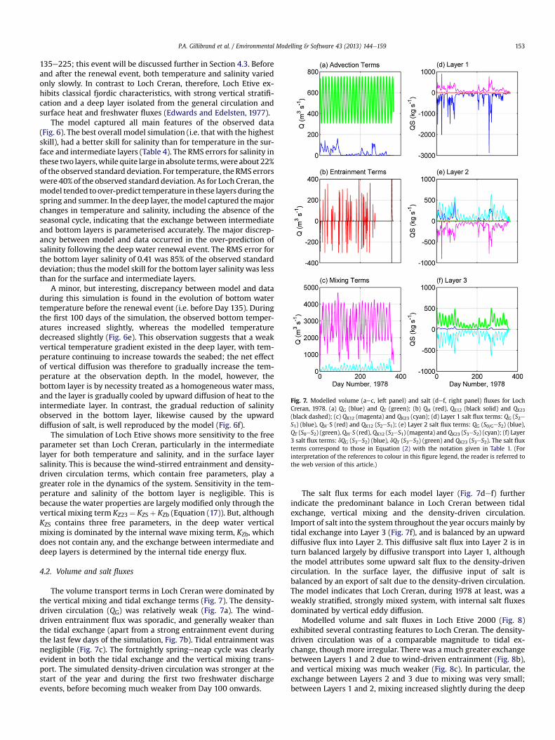
Fig. 7. Modelled volume (aec, left panel) and salt (def, right panel) fluxes for LochCreran, 1978. (a) QG (blue) and QT (green); (b) QH (red), QE12 (black solid) and QE23

(black dashed); (c) QK12 (magenta) and QK23 (cyan); (d) Layer 1 salt flux terms: QG (S2eS1) (blue), QH$S (red) and QK12 (S2eS1); (e) Layer 2 salt flux terms: QG (S0/GeS2) (blue),QT (S0eS2) (green), QH$S (red), QK12 (S2eS1) (magenta) and QK23 (S3eS2) (cyan); (f) Layer3 salt flux terms: dQG (S3eS2) (blue), dQT (S3eS2) (green) and QK23 (S3eS2). The salt fluxterms correspond to those in Equation (2) with the notation given in Table 1. (Forinterpretation of the references to colour in this figure legend, the reader is referred tothe web version of this article.)

P.A. Gillibrand et al. / Environmental Modelling & Software 43 (2013) 144e159 153

135e225; this event will be discussed further in Section 4.3. Beforeand after the renewal event, both temperature and salinity variedonly slowly. In contrast to Loch Creran, therefore, Loch Etive ex-hibits classical fjordic characteristics, with strong vertical stratifi-cation and a deep layer isolated from the general circulation andsurface heat and freshwater fluxes (Edwards and Edelsten, 1977).

The model captured all main features of the observed data(Fig. 6). The best overall model simulation (i.e. that with the highestskill), had a better skill for salinity than for temperature in the sur-face and intermediate layers (Table 4). The RMS errors for salinity inthese two layers,while quite large in absolute terms,were about 22%of the observed standard deviation. For temperature, the RMS errorswere 40% of the observed standard deviation. As for Loch Creran, themodel tended toover-predict temperature in these layers during thespring and summer. In the deep layer, themodel captured themajorchanges in temperature and salinity, including the absence of theseasonal cycle, indicating that the exchange between intermediateand bottom layers is parameterised accurately. The major discrep-ancy between model and data occurred in the over-prediction ofsalinity following the deep water renewal event. The RMS error forthe bottom layer salinity of 0.41 was 85% of the observed standarddeviation; thus themodel skill for the bottom layer salinity was lessthan for the surface and intermediate layers.

A minor, but interesting, discrepancy between model and dataduring this simulation is found in the evolution of bottom watertemperature before the renewal event (i.e. before Day 135). Duringthe first 100 days of the simulation, the observed bottom temper-atures increased slightly, whereas the modelled temperaturedecreased slightly (Fig. 6e). This observation suggests that a weakvertical temperature gradient existed in the deep layer, with tem-perature continuing to increase towards the seabed; the net effectof vertical diffusion was therefore to gradually increase the tem-perature at the observation depth. In the model, however, thebottom layer is by necessity treated as a homogeneous water mass,and the layer is gradually cooled by upward diffusion of heat to theintermediate layer. In contrast, the gradual reduction of salinityobserved in the bottom layer, likewise caused by the upwarddiffusion of salt, is well reproduced by the model (Fig. 6f).

The simulation of Loch Etive shows more sensitivity to the freeparameter set than Loch Creran, particularly in the intermediatelayer for both temperature and salinity, and in the surface layersalinity. This is because the wind-stirred entrainment and density-driven circulation terms, which contain free parameters, play agreater role in the dynamics of the system. Sensitivity in the tem-perature and salinity of the bottom layer is negligible. This isbecause the water properties are largely modified only through thevertical mixing term KZ23 ¼ KZS þ KZb (Equation (17)). But, althoughKZS contains three free parameters, in the deep water verticalmixing is dominated by the internal wave mixing term, KZb, whichdoes not contain any, and the exchange between intermediate anddeep layers is determined by the internal tide energy flux.

4.2. Volume and salt fluxes

The volume transport terms in Loch Creran were dominated bythe vertical mixing and tidal exchange terms (Fig. 7). The density-driven circulation (QG) was relatively weak (Fig. 7a). The wind-driven entrainment flux was sporadic, and generally weaker thanthe tidal exchange (apart from a strong entrainment event duringthe last few days of the simulation, Fig. 7b). Tidal entrainment wasnegligible (Fig. 7c). The fortnightly springeneap cycle was clearlyevident in both the tidal exchange and the vertical mixing trans-port. The simulated density-driven circulation was stronger at thestart of the year and during the first two freshwater dischargeevents, before becoming much weaker from Day 100 onwards.

The salt flux terms for each model layer (Fig. 7def) furtherindicate the predominant balance in Loch Creran between tidalexchange, vertical mixing and the density-driven circulation.Import of salt into the system throughout the year occurs mainly bytidal exchange into Layer 3 (Fig. 7f), and is balanced by an upwarddiffusive flux into Layer 2. This diffusive salt flux into Layer 2 is inturn balanced largely by diffusive transport into Layer 1, althoughthe model attributes some upward salt flux to the density-drivencirculation. In the surface layer, the diffusive input of salt isbalanced by an export of salt due to the density-driven circulation.The model indicates that Loch Creran, during 1978 at least, was aweakly stratified, strongly mixed system, with internal salt fluxesdominated by vertical eddy diffusion.

Modelled volume and salt fluxes in Loch Etive 2000 (Fig. 8)exhibited several contrasting features to Loch Creran. The density-driven circulation was of a comparable magnitude to tidal ex-change, though more irregular. There was a much greater exchangebetween Layers 1 and 2 due to wind-driven entrainment (Fig. 8b),and vertical mixing was much weaker (Fig. 8c). In particular, theexchange between Layers 2 and 3 due to mixing was very small;between Layers 1 and 2, mixing increased slightly during the deep

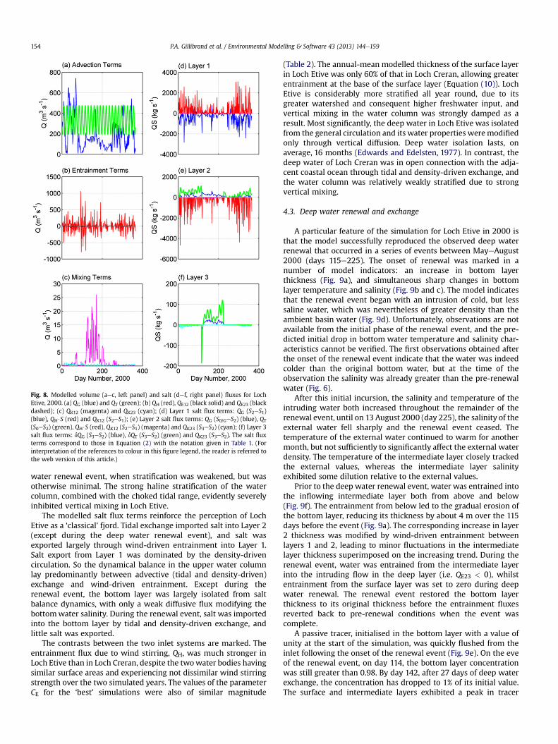
Fig. 8. Modelled volume (aec, left panel) and salt (def, right panel) fluxes for LochEtive, 2000. (a) QG (blue) and QT (green); (b) QH (red), QE12 (black solid) and QE23 (blackdashed); (c) QK12 (magenta) and QK23 (cyan); (d) Layer 1 salt flux terms: QG (S2eS1)(blue), QH$S (red) and QK12 (S2eS1); (e) Layer 2 salt flux terms: QG (S0/GeS2) (blue), QT

(S0eS2) (green), QH$S (red), QK12 (S2eS1) (magenta) and QK23 (S3eS2) (cyan); (f) Layer 3salt flux terms: dQG (S3eS2) (blue), dQT (S3eS2) (green) and QK23 (S3eS2). The salt fluxterms correspond to those in Equation (2) with the notation given in Table 1. (Forinterpretation of the references to colour in this figure legend, the reader is referred tothe web version of this article.)

P.A. Gillibrand et al. / Environmental Modelling & Software 43 (2013) 144e159154

water renewal event, when stratification was weakened, but wasotherwise minimal. The strong haline stratification of the watercolumn, combined with the choked tidal range, evidently severelyinhibited vertical mixing in Loch Etive.

The modelled salt flux terms reinforce the perception of LochEtive as a ‘classical’ fjord. Tidal exchange imported salt into Layer 2(except during the deep water renewal event), and salt wasexported largely through wind-driven entrainment into Layer 1.Salt export from Layer 1 was dominated by the density-drivencirculation. So the dynamical balance in the upper water columnlay predominantly between advective (tidal and density-driven)exchange and wind-driven entrainment. Except during therenewal event, the bottom layer was largely isolated from saltbalance dynamics, with only a weak diffusive flux modifying thebottomwater salinity. During the renewal event, salt was importedinto the bottom layer by tidal and density-driven exchange, andlittle salt was exported.

The contrasts between the two inlet systems are marked. Theentrainment flux due to wind stirring, QH, was much stronger inLoch Etive than in Loch Creran, despite the twowater bodies havingsimilar surface areas and experiencing not dissimilar wind stirringstrength over the two simulated years. The values of the parameterCE for the ‘best’ simulations were also of similar magnitude

(Table 2). The annual-mean modelled thickness of the surface layerin Loch Etive was only 60% of that in Loch Creran, allowing greaterentrainment at the base of the surface layer (Equation (10)). LochEtive is considerably more stratified all year round, due to itsgreater watershed and consequent higher freshwater input, andvertical mixing in the water column was strongly damped as aresult. Most significantly, the deep water in Loch Etive was isolatedfrom the general circulation and its water properties weremodifiedonly through vertical diffusion. Deep water isolation lasts, onaverage, 16 months (Edwards and Edelsten, 1977). In contrast, thedeep water of Loch Creran was in open connection with the adja-cent coastal ocean through tidal and density-driven exchange, andthe water column was relatively weakly stratified due to strongvertical mixing.

4.3. Deep water renewal and exchange

A particular feature of the simulation for Loch Etive in 2000 isthat the model successfully reproduced the observed deep waterrenewal that occurred in a series of events between MayeAugust2000 (days 115e225). The onset of renewal was marked in anumber of model indicators: an increase in bottom layerthickness (Fig. 9a), and simultaneous sharp changes in bottomlayer temperature and salinity (Fig. 9b and c). The model indicatesthat the renewal event began with an intrusion of cold, but lesssaline water, which was nevertheless of greater density than theambient basin water (Fig. 9d). Unfortunately, observations are notavailable from the initial phase of the renewal event, and the pre-dicted initial drop in bottom water temperature and salinity char-acteristics cannot be verified. The first observations obtained afterthe onset of the renewal event indicate that the water was indeedcolder than the original bottom water, but at the time of theobservation the salinity was already greater than the pre-renewalwater (Fig. 6).

After this initial incursion, the salinity and temperature of theintruding water both increased throughout the remainder of therenewal event, until on 13 August 2000 (day 225), the salinity of theexternal water fell sharply and the renewal event ceased. Thetemperature of the external water continued to warm for anothermonth, but not sufficiently to significantly affect the external waterdensity. The temperature of the intermediate layer closely trackedthe external values, whereas the intermediate layer salinityexhibited some dilution relative to the external values.

Prior to the deep water renewal event, water was entrained intothe inflowing intermediate layer both from above and below(Fig. 9f). The entrainment from below led to the gradual erosion ofthe bottom layer, reducing its thickness by about 4 m over the 115days before the event (Fig. 9a). The corresponding increase in layer2 thickness was modified by wind-driven entrainment betweenlayers 1 and 2, leading to minor fluctuations in the intermediatelayer thickness superimposed on the increasing trend. During therenewal event, water was entrained from the intermediate layerinto the intruding flow in the deep layer (i.e. QE23 < 0), whilstentrainment from the surface layer was set to zero during deepwater renewal. The renewal event restored the bottom layerthickness to its original thickness before the entrainment fluxesreverted back to pre-renewal conditions when the event wascomplete.

A passive tracer, initialised in the bottom layer with a value ofunity at the start of the simulation, was quickly flushed from theinlet following the onset of the renewal event (Fig. 9e). On the eveof the renewal event, on day 114, the bottom layer concentrationwas still greater than 0.98. By day 142, after 27 days of deep waterexchange, the concentration has dropped to 1% of its initial value.The surface and intermediate layers exhibited a peak in tracer

Fig. 10. Time series of modelled mixing parameters for Loch Creran 1978 and LochEtive 2000: (a, b) inter-layer density difference (kg m�3); (c, d) bulk RichardsonNumber, RiB; (e, f) vertical diffusivity KZij (cm2 s�1); (g, h) the function (1 þ gRiB)l forcalculated values of RiB in each system. In (a)e(f), the density difference, RichardsonNumber and diffusivity between surface and intermediate layers are shown in blue,and those between intermediate and bottom layers in green. Note the different x-axisscales for (a)e(f) and (g)e(h). (For interpretation of the references to colour in thisfigure legend, the reader is referred to the web version of this article.)

Fig. 9. Time series of modelled parameters for Loch Etive 2000: (a) layer thickness(m); (b, c, d) temperature (T �C), salinity and density (st) in the intermediate andbottom layers; (e) passive tracer concentrations arising from an initial distribution ofunity in the bottom layer, and zero in the surface and intermediate layers; (f) tidalentrainment terms QE12 (blue) and QE23 (green) (m3 s�1). In (a)e(e), parameters forlayers 1e3 are drawn in blue, green and red respectively. In (bed), the time series of T,S and st at the open boundary are overlain in grey. (For interpretation of the referencesto colour in this figure legend, the reader is referred to the web version of this article.)

P.A. Gillibrand et al. / Environmental Modelling & Software 43 (2013) 144e159 155

concentration during the renewal event, as tracer was lifted up intothe overlying water before being exported from the inlet. The tracertime series provide an indication of the rapid replacement of bot-tom water during renewal events.

4.4. Vertical mixing

The volume and salt fluxes discussed in Section 4.2 reveal a keydifference between the two modelled inlets. While the simulationof Loch Creran in 1978 featured strong vertical mixing and ex-change between the layers, diffusive fluxes in Loch Etive wereminimal during 2000. The stratification in Loch Etive was consis-tently stronger than that in Loch Creran (Fig. 10), due to the greaterinput of freshwater per unit surface area of the inlet, and resulted inbulk Richardson numbers that were two or three orders of mag-nitudes greater (Fig. 10c and d). Vertical mixing coefficients weretherefore strongly damped in Loch Etive compared to Loch Creran(Fig. 10e and f). In both inlets, the mixing between layers 2 and 3was dominated by the background mixing term, KZb, as the strati-fication was sufficiently strong to largely suppress the shear-drivencomponent (Fig. 10g and h).

Annual-meanmodelled diffusivities during 1978 for Loch Creranwere 11 cm2 s�1 and 14 cm2 s�1 for the upper and lower interfacesrespectively, whereas for Loch Etive in 2000 the correspondingvalues were 0.02 and 0.04 cm2 s�1 respectively. The modelledturbulent mixing was therefore on average roughly five hundredtimes greater in Loch Creran than in Loch Etive.

The mean vertical diffusivity between layers 2 and 3 for LochEtive during autumn and winter, i.e. in the absence of the deepwater renewal event, can be converted into a vertical mixing rate of0.35 m3 s�1. This can be recalculated as an exchange rate (E ¼ Q/V)of 0.05 year�1. By way of comparison, Edwards and Edelsten (1977)calculated the vertical exchange rate in Loch Etive deep waterduring stagnation periods from 1971 to 1973, and obtained valuesof 0.2 year�1 for salt and 0.5 year�1 for temperature. Our value isthus considerably lower than theirs, yet the modelled rate ofchange of salinity during the period before and after renewal eventin 2000 compares well with the observations (Fig. 6f). This raisesthe question, as yet unresolved, of whether the mixing regime inLoch Etive has changed since the early 1970s, or whether the dif-ference in estimated diffusion rates is due to the differentmethodologies.

P.A. Gillibrand et al. / Environmental Modelling & Software 43 (2013) 144e159156

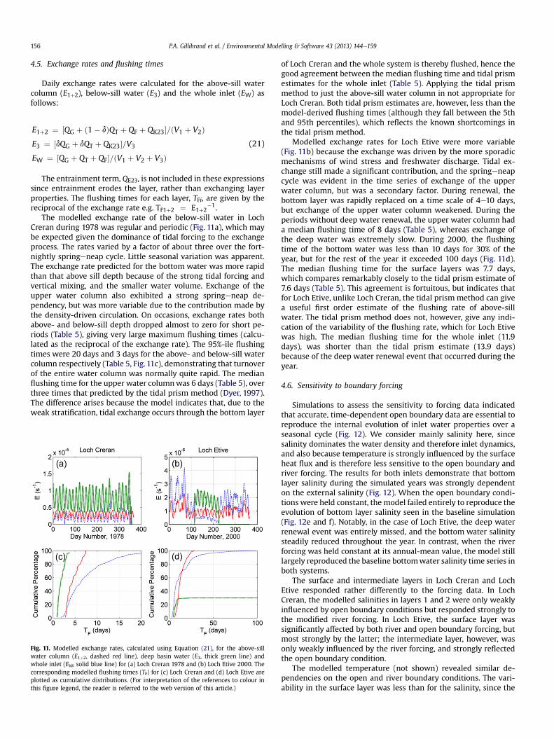
4.5. Exchange rates and flushing times

Daily exchange rates were calculated for the above-sill watercolumn (E1þ2), below-sill water (E3) and the whole inlet (EW) asfollows:

E1þ2 ¼ ½QG þ ð1� dÞQT þ QF þ QK23�=ðV1 þ V2ÞE3 ¼ ½dQG þ dQT þ QK23�=V3

EW ¼ ½QG þ QT þ QF�=ðV1 þ V2 þ V3Þ(21)

The entrainment term, QE23, is not included in these expressionssince entrainment erodes the layer, rather than exchanging layerproperties. The flushing times for each layer, TFi, are given by thereciprocal of the exchange rate e.g. TF1þ2 ¼ E1þ2

�1.The modelled exchange rate of the below-sill water in Loch

Creran during 1978 was regular and periodic (Fig. 11a), which maybe expected given the dominance of tidal forcing to the exchangeprocess. The rates varied by a factor of about three over the fort-nightly springeneap cycle. Little seasonal variation was apparent.The exchange rate predicted for the bottom water was more rapidthan that above sill depth because of the strong tidal forcing andvertical mixing, and the smaller water volume. Exchange of theupper water column also exhibited a strong springeneap de-pendency, but was more variable due to the contribution made bythe density-driven circulation. On occasions, exchange rates bothabove- and below-sill depth dropped almost to zero for short pe-riods (Table 5), giving very large maximum flushing times (calcu-lated as the reciprocal of the exchange rate). The 95%-ile flushingtimes were 20 days and 3 days for the above- and below-sill watercolumn respectively (Table 5, Fig. 11c), demonstrating that turnoverof the entire water column was normally quite rapid. The medianflushing time for the upper water columnwas 6 days (Table 5), overthree times that predicted by the tidal prism method (Dyer, 1997).The difference arises because the model indicates that, due to theweak stratification, tidal exchange occurs through the bottom layer

Fig. 11. Modelled exchange rates, calculated using Equation (21), for the above-sillwater column (E1þ2, dashed red line), deep basin water (E3, thick green line) andwhole inlet (EW, solid blue line) for (a) Loch Creran 1978 and (b) Loch Etive 2000. Thecorresponding modelled flushing times (TF) for (c) Loch Creran and (d) Loch Etive areplotted as cumulative distributions. (For interpretation of the references to colour inthis figure legend, the reader is referred to the web version of this article.)

of Loch Creran and the whole system is thereby flushed, hence thegood agreement between the median flushing time and tidal prismestimates for the whole inlet (Table 5). Applying the tidal prismmethod to just the above-sill water column in not appropriate forLoch Creran. Both tidal prism estimates are, however, less than themodel-derived flushing times (although they fall between the 5thand 95th percentiles), which reflects the known shortcomings inthe tidal prism method.

Modelled exchange rates for Loch Etive were more variable(Fig. 11b) because the exchange was driven by the more sporadicmechanisms of wind stress and freshwater discharge. Tidal ex-change still made a significant contribution, and the springeneapcycle was evident in the time series of exchange of the upperwater column, but was a secondary factor. During renewal, thebottom layer was rapidly replaced on a time scale of 4e10 days,but exchange of the upper water column weakened. During theperiods without deep water renewal, the upper water column hada median flushing time of 8 days (Table 5), whereas exchange ofthe deep water was extremely slow. During 2000, the flushingtime of the bottom water was less than 10 days for 30% of theyear, but for the rest of the year it exceeded 100 days (Fig. 11d).The median flushing time for the surface layers was 7.7 days,which compares remarkably closely to the tidal prism estimate of7.6 days (Table 5). This agreement is fortuitous, but indicates thatfor Loch Etive, unlike Loch Creran, the tidal prism method can givea useful first order estimate of the flushing rate of above-sillwater. The tidal prism method does not, however, give any indi-cation of the variability of the flushing rate, which for Loch Etivewas high. The median flushing time for the whole inlet (11.9days), was shorter than the tidal prism estimate (13.9 days)because of the deep water renewal event that occurred during theyear.

4.6. Sensitivity to boundary forcing

Simulations to assess the sensitivity to forcing data indicatedthat accurate, time-dependent open boundary data are essential toreproduce the internal evolution of inlet water properties over aseasonal cycle (Fig. 12). We consider mainly salinity here, sincesalinity dominates the water density and therefore inlet dynamics,and also because temperature is strongly influenced by the surfaceheat flux and is therefore less sensitive to the open boundary andriver forcing. The results for both inlets demonstrate that bottomlayer salinity during the simulated years was strongly dependenton the external salinity (Fig. 12). When the open boundary condi-tions were held constant, the model failed entirely to reproduce theevolution of bottom layer salinity seen in the baseline simulation(Fig. 12e and f). Notably, in the case of Loch Etive, the deep waterrenewal event was entirely missed, and the bottom water salinitysteadily reduced throughout the year. In contrast, when the riverforcing was held constant at its annual-mean value, the model stilllargely reproduced the baseline bottomwater salinity time series inboth systems.

The surface and intermediate layers in Loch Creran and LochEtive responded rather differently to the forcing data. In LochCreran, the modelled salinities in layers 1 and 2 were only weaklyinfluenced by open boundary conditions but responded strongly tothe modified river forcing. In Loch Etive, the surface layer wassignificantly affected by both river and open boundary forcing, butmost strongly by the latter; the intermediate layer, however, wasonly weakly influenced by the river forcing, and strongly reflectedthe open boundary condition.

The modelled temperature (not shown) revealed similar de-pendencies on the open and river boundary conditions. The vari-ability in the surface layer was less than for the salinity, since the

Table 5Statistics from each simulation of the calculated exchange rate, E (�10�6 s�1), and the flushing time, TF (days), for the above-sill water column (Layers 1þ2) and the basinwater(Layer 3). The exchange rates were calculated using Equation (21). Parameters shown are the minimum (Min), 5th percentile (P5), median (Med), 95th percentile (P95) andmaximum. The flushing times for each system as calculated using the tidal prism method (Dyer, 1997), are also presented for comparison, and were calculated using annual-mean volumes of the above-sill water column and whole inlet.

E (�10�6 s�1) TF (days) TF (prism)(days)

Min P5 Med P95 Max Min P5 Med P95 Max

Loch Creran 1978Layer 1 þ 2 0.000 0.585 1.924 4.386 7.893 1.5 2.6 6.0 19.8 1149 1.6Layer 3 0.000 3.555 6.831 11.757 15.439 0.7 1.0 1.7 3.3 Inf e

Whole 1.552 1.566 2.810 3.941 4.398 2.6 2.9 4.1 7.4 7.5 3.1Loch Etive 2000Layer 1 þ 2 0.112 0.262 1.506 3.046 4.228 2.7 3.8 7.7 44.1 99.5 7.6Layer 3 0.000 0.000 0.002 2.222 2.620 4.4 5.2 6971 34,548 80,013 e

Whole 0.405 0.481 0.974 1.610 2.301 5.0 6.9 11.9 22.8 28.6 13.9

P.A. Gillibrand et al. / Environmental Modelling & Software 43 (2013) 144e159 157

surface temperature was also strongly influenced by the surfaceheat flux. In the intermediate layer, temperature in both systemswas strongly influenced by the open boundary and only weaklyaffected by river forcing. In the deep layer, the open boundaryforcing dominated basin conditions.

Overall, it is evident that realistic data for both the river inputsand the open boundary are required for the model to producepredicted time series that are comparable with observations (aswas demonstrated for the baseline time series).

Fig. 12. Results from the forcing sensitivity simulations. Predicted salinity from sim-ulations with full forcing (‘Baseline’), constant open boundary conditions (‘OBC con-stant’), constant river flow (‘River constant’) and with both OBC and river constant areshown for each model layer in Loch Creran (a, c, e) and Loch Etive (b, d, f).

5. Discussion

Regular observations of temperature and salinity over a seasonalcycle in Loch Creran and Loch Etive, albeit collected over differentyears, revealed contrasting hydrography in the two systems, withthe former being weakly stratified and the latter strongly stratified.The application of the ACExR model to these two fjordic RREssuccessfully reproduced the distinct hydrographic conditions, withRMS errors for temperature and salinity typically less than 1 �C andof the order of 1 respectively. These RMS errors are comparable toother simple models of circulation and mixing in RREs for whicherror calculations have been published (e.g. Liungman, 2000;Babson et al., 2006). In addition, the model provided quantitativeestimates of the dynamic processes that result from, and sustain,those hydrographic conditions, allowing us to characterise thesystems. According to the model, Loch Creran behaved as a well-mixed box, with weak stratification maintained by strong verticaldiffusion and volume exchange between the inlet and coastal wa-ters dominated by tidal forcing. In contrast, Loch Etive exhibitedclassical fjordic three-layer hydrography and dynamics, with strongstratification, weak vertical diffusion and a density-driven circula-tion comparable in strength to tidal exchange.

The focus of this paper has been the application of the ACExRmodel to two fjordic RREs in Scotland. However, we believe themodel can be applied to awider range of RRE types such as rias, voesand lagoons. Themodel can operatewith twoor three layers,with orwithout a constricted entrance, and has been provisionally appliedto Sandsound Voe, a sill-less inlet in the Shetland Islands off NorthScotland. The model as currently conceived assumes that only theintermediate layer is tidally exchanged and that the surface layeronly experiences tidal forcing through secondary mechanisms(entrainment and mixing). For well-mixed and partially-mixed es-tuaries, themodelmay be limited in its applicabilitywithout furtherrefinement; certainly it is currently untested in those particularenvironments. In estuaries where flushing is dominated by strongriver input, the traditional freshwater-salinity boxmodels describedby Officer (1980) may remain a better tool. However, Officer (1980)also describes the box model concept as a balance between an up-streamfluxof salt due to tidal exchange and the net circulation and adownstream flux due to river flow, which is not inconsistent withour conceptual model. A further modification required to make themodel suitable for other types of RRE, particularly those in lowerlatitudes, is to incorporate evaporation and precipitation processes,the lack ofwhichmay have contributed to the slight over-predictionof surface layer temperatures in both simulations reported here.

In order to facilitate wider application of the model to othersystems, the availability and influence of the open boundary dataneeds to be further considered. A simple sensitivity experimentdescribed here revealed the importance of realistic boundary

P.A. Gillibrand et al. / Environmental Modelling & Software 43 (2013) 144e159158

forcing to reproduce the evolution of internal water propertiesaccurately, particularly in the deeper layers. This is not surprisinggiven the connection between the tidally-exchanged (intermediateor bottom) layer and the external water. The use of a climatology ofU.K. coastal temperature and salinity, developed by the U.K. Hy-drographic Office, to drive the model is being investigated. Thedisadvantage of using a climatology is that short-term events, suchas a freshening of coastal salinity due to high rainfall, which maystrongly influence conditions inside coastal inlets, are lost in theaveraging process. Whilst weakening direct comparisons betweenmodel predictions and observations, it is not clear however thatsuch events, despite modifying internal water properties, havemuch impact on the flushing and exchange of the inlet, which re-mains the ultimate objective of the model. The exchange of thesurface layers is dependent on both the density-driven circulationand tidal exchange terms (Equation (21)), and only the former isdependent on water properties, as is the vertical mixing termindirectly. The errors introduced into the model simulations ofwater properties and exchange rates by using a climatologicalboundary condition need to be assessed further before widerapplication can be justified. In addition, more case studies are beingconducted, and a further option is to use output from the currentgeneration of continental shelf hydrodynamic models (e.g. Wakelinet al., 2009) to drive the box model.

One of the key outcomes of the model is the ability to calculatethe mean and daily variability of the flushing time of an RRE. Theflushing time (or variations thereof, such as turnover time andresidence time) is a key parameter used by coastal managers to tryand ensure sustainable development of inshore waters. In bothsystems studied here, the predicted flushing times for the com-bined surface and intermediate layers were largely consistent withvalues estimated using the traditional tidal prism method (Dyer,1997). The tidal prism method has generally been considered tooverestimate exchange rates, due to the inherent assumptions ofcomplete vertical mixing every tidal cycle and fully efficient ex-change of water between consecutive ebb and flood tides. Our re-sults indicate that, though simplistic, the prism-based resultingflushing times for Loch Creran and Loch Etive were not unreason-able. The inefficiencies of tidal exchange, ignored by the tidal prismmethod, are compensated to some extent by the additional ex-change prompted by vertical mixing and the density-driven cir-culation. This provides some confidence in the historicalapplication of the simple ECE model (Gillibrand and Turrell, 1997;Tett et al., 2003; Amundrud et al., 2009) used to advise on aqua-culture development in Scotland.

Whereas the tidal prism method of calculating exchange pro-vides a quasi-constant flushing rate (depending whether vari-ability in tidal range is incorporated), the present model illustratesthe temporal variability in the net volume exchange of the surfaceand intermediate layers. That variability ranged over two orders ofmagnitude, seasonally-varying information that would enableregulators and managers to make more informed decisions aboutassimilative capacity. For example, surface layer exchange may beweakest in summer, when river flows and wind stress are mini-mal; regulators may want to set aquaculture production limitsbased on summer exchange rates to reduce the potential forsummer eutrophication. In the two inlets modelled here, theseasonal variation in flushing was rather small, reflecting thedominance of tidally-driven exchange. The coupling of the ACExRmodel with the LESV ecological box model (Portilla et al., 2009)will allow regulators to investigate and rapidly test the ecosystemresponse to different production limits (Tett et al., 2011). Thisapproach of using simple models to manage aquaculture devel-opment has been adopted in Norway (e.g. Ervik et al., 1997;Stigebrandt et al., 2004). The ACExReLESV models are written in

MATLAB� scripts, making them easily available to academics andregulators with access to MATLAB software, with quick run-timeson a desktop computer.

A wide variety of fluid dynamic processes occur in RREs,particularly where stratified tidal flow interacts with topography(Farmer and Freeland, 1983; Inall and Gillibrand, 2010). Repre-senting some of these complex processes through simple analyticalexpressions inevitably leads to a loss of realism in model simula-tions and introduces errors into model-data comparisons. Ifimproved understanding of those processes is required, orspatially-resolved maps of the water circulation desired, then thespatially-averaged ACExR model will not suffice; for those pur-poses, a full three-dimensional hydrodynamic model must be used.Nevertheless, effective resource management in these valuableenvironments and ecosystems requires appropriate tools that allowregulators and managers to control development at sustainablelevels. Previous models used for this purpose, in Scotland forexample (Gillibrand and Turrell, 1997), while having served theirpurpose, are no longer adequate (Amundrud et al., 2009), inparticular because they did not capture seasonal and shorter-termvariability in the exchange of the system, which has importantimplications because of the seasonal nature of emissions fromaquaculture for example. Although still relatively simple, the ACExRmodel described here improves the representation of physicalprocesses in these regions compared to previous models intendedfor regulation and management (e.g. Gillibrand and Turrell, 1997;Ross et al., 1993, 1994). The ACExR, coupled with the LESV model(Portilla et al., 2009; Tett et al., 2011), therefore offers a potentiallysignificant step forward towards improved management tools forRegions of Restricted Exchange.

Acknowledgements

Meteorological data were obtained from the UK MeteorologicalOffice through the British Atmospheric Data Centre (BADC). Riverflow data were supplied by the Scottish Environment ProtectionAgency (SEPA). The UK Hydrographic Office (UKHO) provided theclimatology of coastal temperature and salinity data. Marie Porterprocessed the data from Loch Creran and Loch Etive. We thank ProfAnders Stigebrandt, Dr Matt Gubbins and Dr Trisha Amundrud fortheir advice and suggestions during the course of the project. Thiswork was funded by the Scottish Aquaculture Research Forumcontract SARF012. We thank two anonymous reviewers for theirhelpful and constructive comments.

References

Amundrud, T.L., Greathead, C., Gubbins, M.J., Davies, I.M., 2009. Nutrient releasefrom coastal aquaculture: the importance of temporal aspects in species-specific production cycles. Aquacult. Res. 40, 1563e1566.

Arneborg, L., 2004. Turnover times for the water above sill level in Gullmar Fjord.Cont. Shelf Res. 24, 443e460.

Babson, A.L., Kawase, M., MacCready, P., 2006. Seasonal and interannual variabilityin the circulation of Puget Sound, Washington: a box model study. Atmosphere-Ocean 44, 29e45.

Black, K.D., 2001. Environmental Impacts of Aquaculture. Sheffield Academic Press,Sheffield, 214 pp.

Booth, D.A., 1987. Some consequences of a flood tide front in Loch Creran. Est. Coast.Shelf Sci. 24, 363e375.

Cottier, F.R., Inall, M.E., Griffiths, C.R., 2004. Seasonal variations in internal waveenergy in a Scottish sea loch. Ocean Dyn. 54, 340e347.

Dyer, K.R., 1997. Estuaries: a Physical Introduction, second ed. John Wiley & Sons,195 pp.

Edwards, A., Edelsten, D.J., 1977. Deep water renewal of Loch Etive: a three basinScottish fjord. Est. Coast. Mar. Sci. 5, 575e595.

Edwards, A., Sharples, F., 1986. Scottish Sea Lochs: a Catalogue. Scottish MarineBiological Association, Oban, U.K, 110 pp.

Ervik, A., Kupta Hansen, P., Aure, J., Stigebrandt, A., Johannessen, P., Jahnsen, T., 1997.Regulating the local environmental impact of intensive marine fish farming. I.

P.A. Gillibrand et al. / Environmental Modelling & Software 43 (2013) 144e159 159

The concept of the MOM system (modelling-ongrowing fish farms-monitoring).Aquaculture 158, 85e94.

Fairall, C.W., Bradley, E.F., Rogers, D.P., Edson, J.B., Young, G.S., 1996. Bulk parame-terization of air-sea fluxes for tropical ocean-global atmosphere coupled-oceanatmosphere response experiment. J. Geophys. Res. 101, 3747e3764.

Farmer, D., Freeland, H., 1983. The physical oceanography of fjords. J. Phys. Ocean-ogr. 12, 147e220.

Gade, H.G., Edwards, A., 1980. Deep water renewal in fjords. In: Freeland, H.J.,Farmer, D.M., Levings, C.D. (Eds.), Fjord Oceanography. Plenum Press, London,pp. 453e489.

Gill, A.E., 1982. Atmosphere-ocean Dynamics. Academic Press, New York, 662 pp.Gillibrand, P.A., Turrell, W.R., 1997. The use of simple models in the regulation of the

impactoffish farmsonwaterquality inScottish sea lochs.Aquaculture 159, 33e46.Inall, M.E., Gillibrand, P.A., 2010. The physics of mid-latitude fjords: a review. In:

Howe, J.A., Austin, W.E.N., Forwick, M., Paetzel, M. (Eds.), Fjord Systems andDynamics. Geological Society, London, Special Publications, vol. 344, pp. 17e33.

Inall, M.E., Cottier, F.R., Griffiths, C., Rippeth, T.P., 2004. Sill dynamics and energytransformation in a jet fjord. Ocean Dyn. 54, 307e314.

Inall, M.E., Rippeth, T.P., 2002. Dissipation of tidal energy and associated mixing in awide fjord. Env. Fluid Mech. 2, 219e240.

Inall, M.E., Rippeth, T.P., Griffiths, C., Wiles, P., 2005. Evolution and distribution ofTKE production and dissipation within stratified flow over topography. Geohys.Res. Lett. 32, L08607. http://dx.doi.org/10.1029/2004GL022289.

Knauss, J.A., 1996. Introduction to Physical Oceanography, second ed. Prentice-Hall,New Jersey, 309 pp.

Li, Ming, Gargett, A.E., Denman, K., 1999. Seasonal and interannual variability ofestuarine circulation in a box model of the Strait of Georgia and Juan de FucaStrait. Atmosphere-Ocean 37, 1e19.

Liungman, O., 2000. Tidally forced internal wave mixing in a k- 3model frameworkapplied to fjord basins. J. Phys. Oceanogr. 30, 352e368.

Lozovatsky, I.D., Roget, E., Fernando, H.J.S., Figueroa,M., Shapovalov, S., 2006. Shearedturbulence in a weakly stratified upper ocean. Deep Sea Res. 53, 387e407.

Munk, W.H., Anderson, E.R., 1948. A note on the theory of the thermocline. J. Mar.Res. 26, 24e33.

Officer, C.B., 1980. Box models revisited. In: Hamilton, P., MacDonald, K.B. (Eds.),Estuarine and Wetland Processes with Emphasis on Modeling. Plenum Press,New York, NY, pp. 65e114.

Pawlowicz, R., Riche, O., Halverson, M., 2007. The circulation and residence time ofthe Strait of Georgia using a simple mixing-box approach. Atmosphere-Ocean45, 173e193.

Portilla, E., Tett, P., Gillibrand, P.A., Inall, M.E., 2009. Description and sensitivityanalysis for the LESV model: water quality variables and the balance oforganisms in a fjordic region of restricted exchange. Ecol. Model. 220,2187e2205.

Princevac, M., Fernando, H.J.S., Whiteman, C.D., 2005. Turbulent entrainment intonatural gravity-driven flows. J. Fluid Mech. 533, 259e268.

Rippeth, T.P., Simpson, J.H., 1996. The frequency and duration of episodes of com-plete vertical mixing in the Clyde Sea. Cont. Shelf Res. 16, 933e947.

Ross, A.H., Gurney, W.S.C., Heath, M.R., Hay, S.J., Henderson, E.W., 1993. A strategicsimulation model of a fjord ecosystem. Limnol. Oceanogr. 38, 128e153.

Ross, A.H., Gurney, W.S.C., Heath, M.R., 1994. A comparative study of the ecosystemdynamics of 4 fjords. Limnol. Oceanogr. 39, 318e343.

Simpson, J.H., Rippeth, T.P., 1993. The Clyde Sea: a model of the seasonal cycle ofstratification and mixing. Est. Coast. Shelf Sci. 37, 129e144.

Stigebrandt, A., 1976. Vertical diffusion driven by internal waves in a sill fjord. J.Phys. Oceanogr. 6, 486e495.

Stigebrandt, A., 1977. On the effect of barotropic current fluctuations on the two-layer transport capacity of a constriction. J. Phys. Oceanogr. 7, 118e122.

Stigebrandt, A., 1980. Some aspects of tidal interaction with fjord constrictions. Est.Coast Mar Sci. 11, 151e166.

Stigebrandt, A., 1981. A mechanism governing the estuarine circulation in deep,strongly stratified fjords. Est. Coast. Shelf Sci. 13, 197e211.

Stigebrandt, A., 1985. A model for the seasonal pycnocline in rotating systems withapplication to the Baltic proper. J. Phys. Oceanogr. 15, 1392e1404.

Stigebrandt, A., 1999. Resistance to barotropic tidal flow in straits by baroclinic wavedrag. J. Phys. Oceanogr. 29, 191e197.

Stigebrandt, A., 2001. FjordEnv e a Water Quality Model for Fjords and OtherInshore Waters. Gothenburg University Report, Sweden, 41 pp.

Stigebrandt, A., Aure, J., 1989. Vertical mixing in the basin waters of fjords. J. Phys.Oceanogr. 19, 917e926.

Stigebrandt, A., Aure, J., Ervik, A., Kupka Hansen, P., 2004. Regulating the localenvironmental impact of intensive marine fish farming: III. A model for esti-mation of the holding capacity in the ModellingeOngrowing fish farme

Monitoring system. Aquaculture, 239e261.Strang, E.J., Fernando, H.J.S., 2001. Entrainment and mixing in stratified shear flows.

J. Fluid Mech. 428, 349e386.Tett, P., Gilpin, L., Svendsen, H., Erlandsson, C.P., Larsson, U., Kratzer, S., Fouilland, E.,

Janzen, C., Lee, J.-Y., Grenz, C., Newton, A., Ferreira, J.G., Fernandes, T., Scory, S.,2003. Eutrophication and some European waters of restricted exchange. Cont.Shelf Res. 23, 1635e1671.

Tett, P., Portilla, E., Gillibrand, P.A., Inall, M.E., 2011. Carrying and assimilativecapacities: the ACExR-LESV model for sea-loch aquaculture. Aquacult. Res. 42,51e67.

Turner, J.S., 1986. Turbulent entrainment: the development of the entrainmentassumption, and its application to geophysical flows. J. Fluid Mech. 173,431e471.

Tyler, I.D., 1983. A Carbon Budget for Creran, a Scottish Sea Loch. Unpublished PhDthesis, University of Strathclyde, Glasgow.

Wakelin, S.L., Holt, J.T., Proctor, R., 2009. The influence of initial conditions and openboundary conditions on shelf circulation in a 3D ocean-shelf model of the NorthEast Atlantic. Ocean Dyn. 59, 67e81.

Wells, M.G., van Heijst, G.-J.F., 2003. A model of tidal flushing of an estuary bydipole formation. Dyn. Atmos. Oceans 37, 223e244.

Willmott, C.J., Ackleson, S.G., Davis, R.E., Feddema, J.J., Klink, K.M., Legates, D.R.,O’Donnell, J., Rowe, C.M., 1985. Statistics for evaluation and comparison ofmodels. J. Geophys. Res. 90, 8995e9005.